mathematics

Article

Computation of Probability Associated withAnderson–Darling Statistic

Lorentz Jäntschi 1,2 ID and Sorana D. Bolboacă 3,* ID

1 Department of Physics and Chemistry, Technical University of Cluj-Napoca, Muncii Blvd. No. 103-105,Cluj-Napoca 400641, Romania; lorentz.jantschi@gmail.com

2 Doctoral Studies, Babes-Bolyai University, Mihail Kogălniceanu Str., No. 1, Cluj-Napoca 400028, Romania3 Department of Medical Informatics and Biostatistics, Iuliu Hatieganu University of Medicine and Pharmacy,

Louis Pasteur Str., No. 6, Cluj-Napoca 400349, Romania* Correspondence: sbolboaca@umfcluj.ro; Tel.: +40-766-341-408

Received: 14 April 2018; Accepted: 23 May 2018; Published: 25 May 2018�����������������

Abstract: The correct application of a statistical test is directly connected with information relatedto the distribution of data. Anderson–Darling is one alternative used to test if the distribution ofexperimental data follows a theoretical distribution. The conclusion of the Anderson–Darling test isusually drawn by comparing the obtained statistic with the available critical value, which did notgive any weight to the same size. This study aimed to provide a formula for calculation of p-valueassociated with the Anderson–Darling statistic considering the size of the sample. A Monte Carlosimulation study was conducted for sample sizes starting from 2 to 61, and based on the obtainedresults, a formula able to give reliable probabilities associated to the Anderson–Darling statisticis reported.

Keywords: Anderson–Darling test (AD); probability; Monte Carlo simulation

1. Introduction

Application of any statistical test is made under certain assumptions, and violation of theseassumptions could lead to misleading interpretations and unreliable results [1,2]. One main assumptionthat several statistical tests have is related with the distribution of experimental or observed data(H0 (null hypothesis): The data follow the specified distribution vs. H1 (alternative hypothesis):The data do not follow the specified distribution). Different tests, generally called “goodness-of-fit”,are used to assess whether a sample of observations can be considered as a sample from agiven distribution. The most frequently used goodness-of-fit tests are Kolmogorov–Smirnov [3,4],Anderson–Darling [5,6], Pearson’s chi-square [7], Cramér–von Mises [8,9], Shapiro–Wilk [10],Jarque–Bera [11–13], D’Agostino–Pearson [14], and Lilliefors [15,16]. The goodness-of-fit tests usedifferent procedures (see Table 1). Alongside the well-known goodness-of-fit test, other methodsbased for example on entropy estimator [17–19], jackknife empirical likelihood [20], on the predictionof residuals [21], or for testing multilevel survival data [22] or multilevel models with binaryoutcomes [23] have been reported in the scientific literature.

Mathematics 2018, 6, 88; doi:10.3390/math6060088 www.mdpi.com/journal/mathematics

Mathematics 2018, 6, 88 2 of 17

Table 1. The goodness-of-fit tests: approaches.

Test Name Abbreviation Procedure

Kolmogorov–Smirnov KSProximity analysis of the empirical distributionfunction (obtained on the sample) and thehypothesized distribution (theoretical)

Anderson–Darling AD How close the points are to the straight lineestimated in a probability graphic

chi-square CS Comparison of sample data distribution with atheoretical distribution

Cramér–von Mises CM Estimation of the minimum distance betweentheoretical and sample probability distribution

Shapiro–Wilk SW

Based on a linear model between the orderedobservations and the expected values of theordered statistics of the standard normaldistribution

Jarque–Bera JBEstimation of the difference between asymmetryand kurtosis of observed data and theoreticaldistribution

D’Agostino–Pearson AP Combination of asymmetry and kurtosis measures

Lilliefors LFA modified KS that uses a Monte Carlo techniqueto calculate an approximation of the samplingdistribution

Tests used to assess the distribution of a dataset received attention from many researchers(for testing normal or other distributions) [24–27]. The normal distribution is of higher importance,since the resulting information will lead the statistical analysis on the pathway of parametric ornon-parametric tests [28–33]. Different normality tests are implemented on various statistical packages(e.g., Minitab—http://www.minitab.com/en-us/; EasyFit—http://www.mathwave.com/easyfit-distribution-fitting.html; Develve—http://develve.net/; r(“nortest” nortest)—https://cran.r-project.org/web/packages/nortest/nortest.pdf; etc.).

Several studies aimed to compare the performances of goodness-of-fit tests. In a Monte Carlosimulation study conducted on the normal distribution, Kolmogorov–Smirnov test has been identifiedas the least powerful test, while opposite Shapiro–Wilks test was identified as the most powerfultest [34]. Furthermore, Anderson–Darling test was found to be the best option among five normalitytests whenever t-statistics were used [35]. More weight to the tails are given by the Anderson–Darlingtest compared to Kolmogorov–Smirnov test [36]. The comparisons between different goodness-of-fittests is frequently conducted by comparing their power [37,38], using or not confidence intervals [39],distribution of p-values [40], or ROC (receiver operating characteristic) analysis [32].

The interpretation of the Anderson–Darling test is frequently made by comparing the AD statisticwith the critical value for a particular significance level (e.g., 20%, 10%, 5%, 2.5%, or 1%) even ifit is known that the critical values depend on the sample size [41,42]. The main problem with thisapproach is that the critical values are available just for several distributions (e.g., normal and Weibulldistribution in Table 2 [43], generalized extreme value and generalized logistic [44], etc.) but couldbe obtained in Monte Carlo simulations [45]. The primary advantage of the Anderson–Darling test isits applicability to test the departure of the experimental data from different theoretical distributions,which is the reason why we decided to identify the method able to calculate its associated p-value as afunction also of the sample size.

D’Augostino and Stephens provided different formulas for calculation of p-values associated tothe Anderson–Darling statistic (AD), along with a correction for small sample size (AD*) [37]. Their

Mathematics 2018, 6, 88 3 of 17

equations are independent of the tested theoretical distribution and highlight the importance of thesample size (Table 3).

Several Excel implementations of Anderson–Darling statistic are freely available to assist theresearcher in testing if data follow, or do not follow, the normal distribution [46–48]. Since almostall distributions are dependent by at least two parameters, it is not expected that one goodness-of-fittest will provide sufficient information regarding the risk of error, because using only one method(one test) gives the expression of only one constraint between parameters. In this regard, the exampleprovided in [49] is illustrative, and shows how the presence of a single outlier induces completedisarray between statistics, and even its removal does not bring the same risk of error as a result ofapplying different goodness-of-fit tests. Given this fact, calculation of the combined probability ofindependent (e.g., independent of the tested distribution) goodness-of-fit tests [50,51] is justified.

Good statistical practice guidelines request reporting the p-value associated with the statisticsof a test. The sample size influences the p-value of statistics, so its reporting is mandatory to assurea proper interpretation of the statistical results. Our study aimed to identify, assess, and implementan explicit function of the p-value associated with the Anderson–Darling statistic able to take intoconsideration both the value of the statistic and the sample size.

Table 2. Anderson–Darling test: critical values according to significance level.

Distribution [Ref] α = 0.10 α = 0.05 α = 0.01

Normal & lognormal [43] 0.631 0.752 1.035

Weibull [43] 0.637 0.757 1.038

Generalized extreme value [44] - - -

n = 10 0.236 0.276 0.370n = 20 0.232 0.274 0.375n = 30 0.232 0.276 0.379n = 40 0.233 0.277 0.381n = 50 0.233 0.277 0.383

n = 100 0.234 0.279 0.387

Generalized logistic [44] - - -

n = 10 0.223 0.266 0.374n = 20 0.241 0.290 0.413n = 30 0.220 0.301 0.429n = 40 0.254 0.306 0.435n = 50 0.258 0.311 0.442

n = 100 0.267 0.323 0.461

Uniform [52] * 1.936 2.499 3.903

* Expressed as upper tail percentiles.

Table 3. Anderson–Darling for small sizes: p-values formulas.

Anderson–Darling Statistic Formula for p-Value Calculation

AD ≥ 0.6 exp (1.2937 − 5.709·(AD*) + 0.0186·(AD*)2)0.34 < AD* < 0.6 exp (0.9177 − 4.279·(AD*) − 1.38·(AD*)2)0.2 < AD* < 0.34 1 − exp (−8.318 + 42.796·(AD*) − 59.938·(AD*)2)

AD* ≤ 0.2 1 − exp (−13.436 + 101.14·(AD*) − 223.73·(AD*)2)

AD∗ = AD(1 + 0.75n + 2.25

n2 ); AD = −n− 1n ·∑

ni=0(2·i− 1)·[ln(F(Xi) + ln(1− F(Xn−i+1))].

Mathematics 2018, 6, 88 4 of 17

2. Materials and Methods

2.1. Anderson–Darling Order Statistic

For a sample Y = (y1, y2, . . . , yn), the data are sorted in ascending order (let X = Sort(Y), andthen X = (x1, x2, . . . , xn) with xi ≤ xi+1 for 0 < i < n, and xi = yσ(i), where σ is a permutation of{1, 2, . . . , n} which makes the X series sorted). Let the CDF be the associated cumulative distributionfunction and InvCDF the inverse of this function for any PDF (probability density function). Theseries P = (p1, p2, . . . , pn) defined by pi = InvCDF(xi) (or Q = (q1, q2, . . . , qn) defined by qi = InvCDF(yi),where the P is the unsorted array, and Q is the sorted array) are samples drawn from a uniformdistribution only if Y (and X) are samples from the distribution with PDF.

At this point, the order statistics are used to test the uniformity of P (or for Q), and for thisreason, the values of X are ordered (in Y). On the ordered probabilities (on P), several statistics can becomputed, and Anderson–Darling (AD) is one of them:

AD = AD(P, n) = −n−n

∑i=1

(2i− 1) ln(pi(1− pn−i+1))

n. (1)

The associated AD statistic for a “perfect” uniform distribution can be computed after splittingthe [0, 1] interval into n equidistant intervals (i/n, with 0 ≤ i ≤ n being their boundaries) and using themiddles of those intervals ri = (2i − 1)/2n:

ADmin(n) = AD(R, n) = −n + 4H1(R, n). (2)

where H1 is the Shannon entropy for R in nats (the units of information or entropy)(H1(R,n) = − Σri·ln(ri)).

Equation (2) gives the smallest possible value for AD. The value of the AD increases with theincrease of the departure between the perfect uniform distribution and the observed distribution (P).

2.2. Monte Carlo Experiment for Anderson–Darling Statistic

The probability associated with a particular value of the AD statistic can be obtained using aMonte Carlo experiment. The AD statistics are calculated for a large enough number of samples (let bem the number of samples), the values are sorted, and then the relative position of the observed value ofthe AD in the series of Monte Carlo-calculated values gives the probability associated with the statisticof the AD test.

It should be noted that the equation linking the statistic and the probability also contains the sizeof the sample, and therefore, the probability associated with the AD value is dependent on n.

Taking into account all the knowledge gains until this point, it is relatively simple to do a MonteCarlo experiment for any order statistic. The only remaining problem is how to draw a sample from auniform distribution in such way as to not affect the outcome. One alternative is to use a good randomgenerator, such as Mersenne Twister [53], and this method was used to generate our samples as analternative to the stratified random approach.

2.3. Stratified Random Strategy

Let us assume that three numbers (t1, t2, t3) are extracted from a [0, 1) interval using MersenneTwister method. Each of those numbers can be <0.5 or ≥0.5, providing 23 possible cases (Table 4).

Mathematics 2018, 6, 88 5 of 17

Table 4. Cases for the half-split of [0, 1).

Class t1 t2 t3 Case

“0” if ti < 0.5“1” if ti ≥ 0.5

0 0 0 10 0 1 20 1 0 30 1 1 41 0 0 51 0 1 61 1 0 71 1 1 8

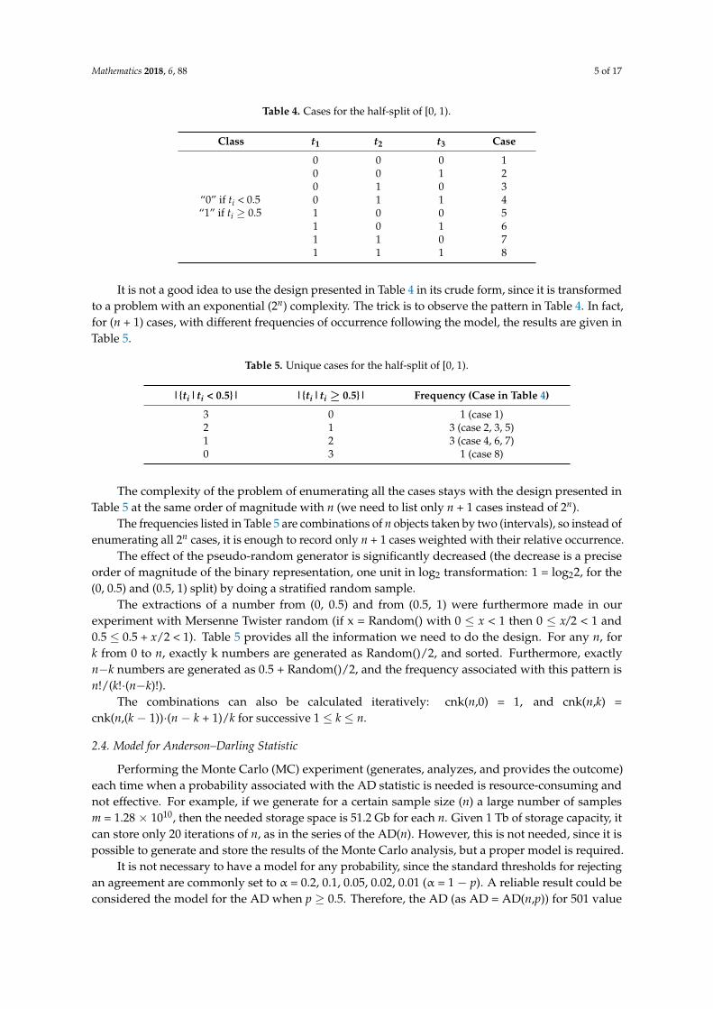
It is not a good idea to use the design presented in Table 4 in its crude form, since it is transformedto a problem with an exponential (2n) complexity. The trick is to observe the pattern in Table 4. In fact,for (n + 1) cases, with different frequencies of occurrence following the model, the results are given inTable 5.

Table 5. Unique cases for the half-split of [0, 1).

|{ti|ti < 0.5}| |{ti|ti ≥ 0.5}| Frequency (Case in Table 4)

3 0 1 (case 1)2 1 3 (case 2, 3, 5)1 2 3 (case 4, 6, 7)0 3 1 (case 8)

The complexity of the problem of enumerating all the cases stays with the design presented inTable 5 at the same order of magnitude with n (we need to list only n + 1 cases instead of 2n).

The frequencies listed in Table 5 are combinations of n objects taken by two (intervals), so instead ofenumerating all 2n cases, it is enough to record only n + 1 cases weighted with their relative occurrence.

The effect of the pseudo-random generator is significantly decreased (the decrease is a preciseorder of magnitude of the binary representation, one unit in log2 transformation: 1 = log22, for the(0, 0.5) and (0.5, 1) split) by doing a stratified random sample.

The extractions of a number from (0, 0.5) and from (0.5, 1) were furthermore made in ourexperiment with Mersenne Twister random (if x = Random() with 0 ≤ x < 1 then 0 ≤ x/2 < 1 and0.5 ≤ 0.5 + x/2 < 1). Table 5 provides all the information we need to do the design. For any n, fork from 0 to n, exactly k numbers are generated as Random()/2, and sorted. Furthermore, exactlyn−k numbers are generated as 0.5 + Random()/2, and the frequency associated with this pattern isn!/(k!·(n−k)!).

The combinations can also be calculated iteratively: cnk(n,0) = 1, and cnk(n,k) =cnk(n,(k − 1))·(n − k + 1)/k for successive 1 ≤ k ≤ n.

2.4. Model for Anderson–Darling Statistic

Performing the Monte Carlo (MC) experiment (generates, analyzes, and provides the outcome)each time when a probability associated with the AD statistic is needed is resource-consuming andnot effective. For example, if we generate for a certain sample size (n) a large number of samplesm = 1.28 × 1010, then the needed storage space is 51.2 Gb for each n. Given 1 Tb of storage capacity, itcan store only 20 iterations of n, as in the series of the AD(n). However, this is not needed, since it ispossible to generate and store the results of the Monte Carlo analysis, but a proper model is required.

It is not necessary to have a model for any probability, since the standard thresholds for rejectingan agreement are commonly set to α = 0.2, 0.1, 0.05, 0.02, 0.01 (α = 1 − p). A reliable result could beconsidered the model for the AD when p ≥ 0.5. Therefore, the AD (as AD = AD(n,p)) for 501 value

Mathematics 2018, 6, 88 6 of 17

of the p from 0.500 to 0.001, and for n from 2 to 61 were extracted, tabulated, and used to developthe model.

A search for a dependency of AD = AD(p) (or p = p(AD)) for a particular n may not reveal anypattern. However, if the value of the statistic is exponentiated (see the ln function in the AD formula),values for the model start to appear (see Figure 1a) after a proper transformation of p. On the otherhand, for a given n, an inconvenience for the AD(p) (or for its inverse, p = p(AD)) is to have on theplot, a non-uniform repartition of the points—for instance, precisely two points for 5 ≤ AD < 6 and144 points for AD < 1. As a consequence, any method trying to find the best fit based on this raw datawill fail because it will give too much weight on the lower part with a much higher concentration ofthe points. The problem is the same for exp(AD) replacing AD (Figure 1b) but is no more the case for1/(1 − p) as a function of exp(AD) (Figure 1c), since the dependence begins to look like a linear one.Figure 1b suggests that a logarithm on both axes will reduce the difference in the concentration ofpoints in the intervals (Figure 1d), but at this point, is not necessary to apply it, since the last spots inFigure 1c may act as “outliers” trailing the slope. A good fit in the rarefied region of high p (and low α)is desired. It is not so important if we will have a 1% error at p = 50%, but is essential not to have a1% error at p = 99% (the error will be higher than the estimated probability, α = 1 − p. Therefore, inthis case (Figure 1c), big numbers (e.g., ~200, 400) will have high values of residuals, and will trail themodel to fit better in the rarefied region.Mathematics 2018, 6, x FOR PEER REVIEW   6 of 6 

   (a)  (b) 

   (c)  (d) 

Figure 1. Probability as function of the AD statistic for a selected case (n = 25)  in the Monte Carlo 

experiment: (a) p = p(AD); (b) p = p(eAD); (c) α‐1 vs. eAD; (d) −ln(α) vs. AD. 

Table 6. Proposed model tested for the AD = AD(p) series for n = 25. SST: Sum of Squares: Total; SSRes: 

Sum of Squares: Residuals; SSE = Sum of Squares Error. 

Coefficient  Value (95% CI)  SE  t‐Value 

a0  4.160 (4.126 to 4.195)  0.017567  237 

a1  −10.327 (−10.392 to −10.263)  0.032902  −314 

a2  9.357 (9.315 to 9.400)  0.02178  430 

a3  −6.147 (−6.159 to −6.135)  0.00601  −1023 

a4  3.4925 (3.4913 to 3.4936)  0.000583  5993 

SST = 1550651, SSRes = 0.0057,  

SSE = 0.0034, r2adj = 0.999999997 

The  analysis of  the  results presented  in Table  6  showed  that  all  coefficients  are  statistically 

significant, and their significance increases from the coefficient of AD1/4 to the coefficient of the AD. 

Furthermore,  the  residuals of  the  regression are with  ten orders of magnitude  less  than  the  total 

residuals (F value = 3.4 × 1010). The adjusted determination coefficient has eight consecutive nines. 

The model is not finished yet, because we need a model that also embeds the sample size (n). 

Inverse powers of n are the best alternatives as already suggested in the literature [43]. Therefore, for 

each coefficient (from a0 to a4), a function penalizing the small samples was used similarly: 

4,4

3,3

2,2

1,1,0

ˆ nbnbnbnbba iiiiii .  (4) 

With these replacements, the whole model providing the probability as a function of AD statistic 

and n is given by Equation (5): 

4

0

4

0

4/,

ˆi j

jiji nxby

,

  (5) 

where ŷ = 1/(1 − p), bi,j = coefficients, x = eAD, n = sample size. 

0.500

0.550

0.600

0.650

0.700

0.750

0.800

0.850

0.900

0.950

1.000

0 1 2 3 4 5 6

0.500

0.550

0.600

0.650

0.700

0.750

0.800

0.850

0.900

0.950

1.000

0 100 200 300 400 500

0

100

200

300

400

500

600

700

800

900

1000

0 100 200 300 400 500

0

1

2

3

4

5

6

7

0 1 2 3 4 5 6

Figure 1. Probability as function of the AD statistic for a selected case (n = 25) in the Monte Carloexperiment: (a) p = p(AD); (b) p = p(eAD); (c) α-1 vs. eAD; (d) −ln(α) vs. AD.

A simple linear regression y ~y = a·x + b for x← eAD and y← α − 1 = 1/(1 − p) will do most ofthe job for providing the values of α associated with the values of the AD. Since the dependence isalmost linear, polynomial or rational functions will perform worse, as proven in the tests. A betteralternative is to feed the model with fractional powers of x. By doing this, the bigger numbers willnot be disfavored (square root of 100 is 10, which is ten times lower than 100, while square root of 1 is1; thus, the weight of the linear component is less affected for bigger numbers). On the other hand,

Mathematics 2018, 6, 88 7 of 17

looking to the AD definition, the probability is raised at a variable power, and therefore, to turn backto it, in the conventional sense of operation, is to do root. Our proposed model is given in Equation (3):

y = a0 + a1x1/4 + a2x2/4 + a3x3/4 + a4x (3)

The statistics associated with the proposed model for data presented in Figure 1 are given inTable 6.

Table 6. Proposed model tested for the AD = AD(p) series for n = 25. SST: Sum of Squares: Total; SSRes:Sum of Squares: Residuals; SSE = Sum of Squares Error.

Coefficient Value (95% CI) SE t-Value

a0 4.160 (4.126 to 4.195) 0.017567 237a1 −10.327 (−10.392 to −10.263) 0.032902 −314a2 9.357 (9.315 to 9.400) 0.02178 430a3 −6.147 (−6.159 to −6.135) 0.00601 −1023a4 3.4925 (3.4913 to 3.4936) 0.000583 5993

SST = 1550651, SSRes = 0.0057,SSE = 0.0034, r2

adj = 0.999999997

The analysis of the results presented in Table 6 showed that all coefficients are statisticallysignificant, and their significance increases from the coefficient of AD1/4 to the coefficient of the AD.Furthermore, the residuals of the regression are with ten orders of magnitude less than the totalresiduals (F value = 3.4 × 1010). The adjusted determination coefficient has eight consecutive nines.

The model is not finished yet, because we need a model that also embeds the sample size (n).Inverse powers of n are the best alternatives as already suggested in the literature [43]. Therefore, foreach coefficient (from a0 to a4), a function penalizing the small samples was used similarly:

ai = b0,i + b1,in−1 + b2,in−2 + b3,in−3 + b4,in−4. (4)

With these replacements, the whole model providing the probability as a function of AD statisticand n is given by Equation (5):

y =4

∑i=0

4

∑j=0

bi,jxi/4n−j, (5)

where y = 1/(1 − p), bi,j = coefficients, x = eAD, n = sample size.

3. Simulation Results

Twenty-five coefficients were calculated for Equation (5) from 60 values associated to sample sizesfrom 2 to 61, based on 500 values of p (0.500 ≤ p ≤ 0.999) and with a step of 0.001. The values of theobtained coefficients along with the related Student t-statistic are given in Table 7.

Mathematics 2018, 6, 88 8 of 17

Table 7. Coefficients of the proposed model and their Student t-values provided in round brackets.

bi,j (ti,j) j = 0 j = 1 j = 2 j = 3 j = 4

i = 0 5.6737(710)

−38.9087(4871)

88.7461(11111)

−179.5470(22479)

199.3247(24955)

i = 1 −13.5729(1699)

83.6500(10473)

−181.6768(22746)

347.6606(43526)

−367.4883(46009)

i = 2 12.0750(1512)

−70.3770(8811)

139.8035(17503)

−245.6051(30749)

243.5784(30496)

i = 3 −7.3190(916)

30.4792(3816)

−49.9105(6249)

76.7476(9609)

−70.1764(8786)

i = 4 3.7309(467)

−6.1885(775)

7.3420(919)

−9.3021(1165)

7.7018(964)

3.1. Stratified vs. Random

The same experiment was conducted with both simple and random stratified Mersenne Twistermethod [53] to assess the magnitude of the increases in the resolution of the AD statistic. The differencesbetween the two scenarios were calculated and plotted in Figure 2.

Mathematics 2018, 6, x FOR PEER REVIEW   7 of 7 

3. Simulation Results 

Twenty‐five coefficients were calculated for Equation (5) from 60 values associated to sample 

sizes from 2 to 61, based on 500 values of p (0.500 ≤ p ≤ 0.999) and with a step of 0.001. The values of 

the obtained coefficients along with the related Student t‐statistic are given in Table 7. 

Table 7. Coefficients of the proposed model and their Student t‐values provided in round brackets. 

bi,j (ti,j)  j = 0  j = 1  j = 2  j = 3  j = 4 

i = 0 5.6737 

(710) 

−38.9087 

(4871) 

88.7461 

(11111) 

−179.5470 

(22479) 

199.3247 

(24955) 

i = 1 −13.5729 

(1699) 

83.6500 

(10473) 

−181.6768 

(22746) 

347.6606 

(43526) 

−367.4883 

(46009) 

i = 2 12.0750 

(1512) 

−70.3770 

(8811) 

139.8035 

(17503) 

−245.6051 

(30749) 

243.5784 

(30496) 

i = 3 −7.3190 

(916) 

30.4792 

(3816) 

−49.9105 

(6249) 

76.7476 

(9609) 

−70.1764 

(8786) 

i = 4 3.7309 

(467) 

−6.1885 

(775) 

7.3420 

(919) 

−9.3021 

(1165) 

7.7018 

(964) 

3.1. Stratified vs. Random 

The same experiment was conducted with both simple and random stratified Mersenne Twister 

method  [53]  to  assess  the magnitude  of  the  increases  in  the  resolution  of  the AD  statistic.  The 

differences between the two scenarios were calculated and plotted in Figure 2. 

red  (−0.07 to −0.05] 

light green  (−0.05 to −0.03] 

blue  (−0.03 to −0.01] 

green  (−0.01 to 0.01] 

cyclam  (0.01 to 0.03] 

yellow  (0.03 to 0.05] 

grey  (0.05–0.07] 

orange  (0.07–0.09] 

Figure 2. The effect in differences between classical and stratified random in calculated AD statistic. 

3.2. Analysis of Residuals 

The  residuals,  defined  as  the  difference  between  the  probability  obtained  by Monte  Carlo 

simulation and the value estimated by the proposed model, without and with transformation (ln and 

respectively log), were analyzed. For each probability (p ranging from 0.500 to 0.999 with a step of 

0.001; 500 values) associated with the statistic (AD) based on the MC simulation for n ranging from 2 

to 61  (60 values), 30,000 distinct pairs  (p, n, AD) were collected and  investigated. The descriptive 

statistics of residuals are presented in Table 8. 

The most frequent value of residuals (~99%) equals with 0.000007 when no transformed data are 

investigated (Figure 3, left‐hand graph). The right‐hand chart in Figure 3 depicted the distribution of 

the  same  data,  but  expressed  in  logarithmical  scale,  showing  a  better  agreement  with  normal 

distribution for the transformed residuals. 

 

 

900

910

920

930

940

950

960

970

980

990

10007 12 17 22 27 32 37 42 47 52

Figure 2. The effect in differences between classical and stratified random in calculated AD statistic.

3.2. Analysis of Residuals

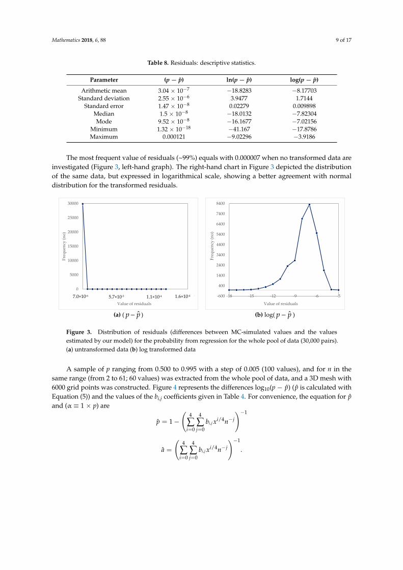
The residuals, defined as the difference between the probability obtained by Monte Carlosimulation and the value estimated by the proposed model, without and with transformation (ln andrespectively log), were analyzed. For each probability (p ranging from 0.500 to 0.999 with a step of0.001; 500 values) associated with the statistic (AD) based on the MC simulation for n ranging from2 to 61 (60 values), 30,000 distinct pairs (p, n, AD) were collected and investigated. The descriptivestatistics of residuals are presented in Table 8.

Mathematics 2018, 6, 88 9 of 17

Table 8. Residuals: descriptive statistics.

Parameter (p − p) ln(p − p) log(p − p)

Arithmetic mean 3.04 × 10−7 −18.8283 −8.17703Standard deviation 2.55 × 10−6 3.9477 1.7144

Standard error 1.47 × 10−8 0.02279 0.009898Median 1.5 × 10−8 −18.0132 −7.82304Mode 9.52 × 10−8 −16.1677 −7.02156

Minimum 1.32 × 10−18 −41.167 −17.8786Maximum 0.000121 −9.02296 −3.9186

The most frequent value of residuals (~99%) equals with 0.000007 when no transformed data areinvestigated (Figure 3, left-hand graph). The right-hand chart in Figure 3 depicted the distributionof the same data, but expressed in logarithmical scale, showing a better agreement with normaldistribution for the transformed residuals.

Mathematics 2018, 6, x FOR PEER REVIEW   8 of 8 

Table 8. Residuals: descriptive statistics. 

Parameter  ( pp ˆ )  ln( pp ˆ )  log( pp ˆ ) 

Arithmetic mean  3.04 × 10−7  −18.8283  −8.17703 

Standard deviation  2.55 × 10−6  3.9477  1.7144 

Standard error  1.47 × 10−8  0.02279  0.009898 

Median  1.5 × 10−8  −18.0132  −7.82304 

Mode  9.52 × 10−8  −16.1677  −7.02156 

Minimum  1.32 × 10−18  −41.167  −17.8786 

Maximum  0.000121  −9.02296  −3.9186 

 

   (a) ( pp ˆ )  (b) log( pp ˆ ) 

Figure  3.  Distribution  of  residuals  (differences  between  MC‐simulated  values  and  the  values 

estimated by our model) for the probability from regression for the whole pool of data (30,000 pairs). 

(a) untransformed data (b) log transformed data  

A sample of p ranging from 0.500 to 0.995 with a step of 0.005 (100 values), and for n in the same 

range (from 2 to 61; 60 values) was extracted from the whole pool of data, and a 3D mesh with 6000 

grid points was constructed. Figure 4 represents  the differences  log10( pp ˆ ) ( p  is calculated with 

Equation (5)) and the values of the bi,j coefficients given in Table 4. For convenience, the equation for 

p and (α ≡ 1 × p) are 

14

0

4

0

4/,1ˆ

i j

jiji nxbp

 

 

14

0

4

0

4/,

ˆ

i j

jiji nxb

.

   

Figure 4 reveals that the calculated Equation (5) and the expected values (from MC simulation 

for AD  = AD(p,n)) differ  less  than  1‰  (−3 on  the  top of  the Z  axis). Even more  than  that, with 

departure from n = 2, and from p = 0.500 to n = 61, or to p = 0.999, the difference dramatically decreases 

to 10−6 (visible on the Z‐axis as −6 moving from n = 2 to n = 61), to 10−9 (visible on the plot visible on 

X‐axis as −9 moving from p = 0.500 to p = 0.995), and even to 10−15 (visible on the plot on Z‐axis as −15 

moving on both from p = 0.500 to p = 0.995 and from n = 2 to n = 61). This behavior shows that the 

model was designed in a way in which the estimation error ( pp ˆ ) would be minimal for small α (α 

close to 0; p close to 1). A regular half‐circle shape pattern, depicted in Figure 4, suggests that an even 

more precise method  than  the one archived by  the proposed model must be done with periodic 

functions. 

0

5000

10000

15000

20000

25000

30000

7.0E‐06 5.7E‐05 1.1E‐04 1.6E‐04

Frequency (no)

Value of residuals

‐600

400

1400

2400

3400

4400

5400

6400

7400

8400

‐18 ‐15 ‐12 ‐9 ‐6 ‐3

Frequency (no)

Value of residuals

7.0×10‐6  5.7×10‐5  1.1×10‐4  1.6×10‐4 

Figure 3. Distribution of residuals (differences between MC-simulated values and the valuesestimated by our model) for the probability from regression for the whole pool of data (30,000 pairs).(a) untransformed data (b) log transformed data

A sample of p ranging from 0.500 to 0.995 with a step of 0.005 (100 values), and for n in thesame range (from 2 to 61; 60 values) was extracted from the whole pool of data, and a 3D mesh with6000 grid points was constructed. Figure 4 represents the differences log10(p − p) (p is calculated withEquation (5)) and the values of the bi,j coefficients given in Table 4. For convenience, the equation for pand (α ≡ 1 × p) are

p = 1−(

4

∑i=0

4

∑j=0

bi,j xi/4n−j

)−1

a =

(4

∑i=0

4

∑j=0

bi,j xi/4n−j

)−1

.

Mathematics 2018, 6, 88 10 of 17Mathematics 2018, 6, x FOR PEER REVIEW   9 of 9 

 

  red  (−18 to −15) 

  light green  (−15 to −12) 

  blue  (−12 to −9) 

  green  (−9 to −6) 

  cyclamen  (−6 to −3)  

Figure 4. 3D plot of the estimation error for data expressed in logarithm scale as function of p (ranging 

from 0.500 to 0.999) and n (ranging from 2 to 61). 

Figure 5 illustrates, more obviously, this pattern with the peak at n = 2 and p = 0.500. 

 

Figure 5. 3D plot of  the estimation error  for untransformed data: Z‐axis show  the 105∙( pp ˆ ) as a 

function of p (ranging from 0.500 to 0.999) and n (ranging from 2 to 61). 

Median of residuals expressed in logarithmic scale indicate that half of the points have exactly 

seven  digits  (e.g.,  0.98900000  vs.  0.98900004).  The  cumulative  frequencies  for  the  residuals 

represented  in  logarithmic scale also show  that 75% have exactly six digits, while over 99% have 

exactly five digits. The agreement between the observed Monte Carlo and the regression model is 

excellent  (r2(n  =  30,000)  =  0.99999) with  a minimum  value  for  the  sum  of  squares  of  residuals 

(0.002485). These results sustain the validity of the proposed model. 

4. Case Study 

Twenty  sets  of  experimental data  (Table  9) were used  to  test  the  hypothesis  of  the  normal 

distribution: 

H0:  The  distribution  of  experimental  data  is  not  significantly  different  from  the  theoretical 

normal distribution. 

H1:  The  distribution  of  experimental  data  is  not  significantly  different  from  the  theoretical 

normal distribution. 

0

10

20

30

40

50

60

0.600.70

0.800.90

1.00

-18

-15

-12

-9

-6

-3

012

2436

4860

0.60

0.70

0.80

0.90

1.00

2

4

6

8

10

Figure 4. 3D plot of the estimation error for data expressed in logarithm scale as function of p (rangingfrom 0.500 to 0.999) and n (ranging from 2 to 61).

Figure 4 reveals that the calculated Equation (5) and the expected values (from MC simulation forAD = AD(p,n)) differ less than 1‰ (−3 on the top of the Z axis). Even more than that, with departurefrom n = 2, and from p = 0.500 to n = 61, or to p = 0.999, the difference dramatically decreases to 10−6

(visible on the Z-axis as−6 moving from n = 2 to n = 61), to 10−9 (visible on the plot visible on X-axis as−9 moving from p = 0.500 to p = 0.995), and even to 10−15 (visible on the plot on Z-axis as −15 movingon both from p = 0.500 to p = 0.995 and from n = 2 to n = 61). This behavior shows that the modelwas designed in a way in which the estimation error (p − p) would be minimal for small α (α close to0; p close to 1). A regular half-circle shape pattern, depicted in Figure 4, suggests that an even moreprecise method than the one archived by the proposed model must be done with periodic functions.

Figure 5 illustrates, more obviously, this pattern with the peak at n = 2 and p = 0.500.

Mathematics 2018, 6, x FOR PEER REVIEW   9 of 9 

 

  red  (−18 to −15) 

  light green  (−15 to −12) 

  blue  (−12 to −9) 

  green  (−9 to −6) 

  cyclamen  (−6 to −3)  

Figure 4. 3D plot of the estimation error for data expressed in logarithm scale as function of p (ranging 

from 0.500 to 0.999) and n (ranging from 2 to 61). 

Figure 5 illustrates, more obviously, this pattern with the peak at n = 2 and p = 0.500. 

 

Figure 5. 3D plot of  the estimation error  for untransformed data: Z‐axis show  the 105∙( pp ˆ ) as a 

function of p (ranging from 0.500 to 0.999) and n (ranging from 2 to 61). 

Median of residuals expressed in logarithmic scale indicate that half of the points have exactly 

seven  digits  (e.g.,  0.98900000  vs.  0.98900004).  The  cumulative  frequencies  for  the  residuals 

represented  in  logarithmic scale also show  that 75% have exactly six digits, while over 99% have 

exactly five digits. The agreement between the observed Monte Carlo and the regression model is 

excellent  (r2(n  =  30,000)  =  0.99999) with  a minimum  value  for  the  sum  of  squares  of  residuals 

(0.002485). These results sustain the validity of the proposed model. 

4. Case Study 

Twenty  sets  of  experimental data  (Table  9) were used  to  test  the  hypothesis  of  the  normal 

distribution: 

H0:  The  distribution  of  experimental  data  is  not  significantly  different  from  the  theoretical 

normal distribution. 

H1:  The  distribution  of  experimental  data  is  not  significantly  different  from  the  theoretical 

normal distribution. 

0

10

20

30

40

50

60

0.600.70

0.800.90

1.00

-18

-15

-12

-9

-6

-3

012

2436

4860

0.60

0.70

0.80

0.90

1.00

2

4

6

8

10

Figure 5. 3D plot of the estimation error for untransformed data: Z-axis show the 105·(p − p) as afunction of p (ranging from 0.500 to 0.999) and n (ranging from 2 to 61).

Median of residuals expressed in logarithmic scale indicate that half of the points have exactlyseven digits (e.g., 0.98900000 vs. 0.98900004). The cumulative frequencies for the residuals representedin logarithmic scale also show that 75% have exactly six digits, while over 99% have exactly fivedigits. The agreement between the observed Monte Carlo and the regression model is excellent(r2(n = 30,000) = 0.99999) with a minimum value for the sum of squares of residuals (0.002485). Theseresults sustain the validity of the proposed model.

Mathematics 2018, 6, 88 11 of 17

4. Case Study

Twenty sets of experimental data (Table 9) were used to test the hypothesis of thenormal distribution:

H1: The distribution of experimental data is not significantly different from the theoreticalnormal distribution.

H2: The distribution of experimental data is not significantly different from the theoreticalnormal distribution.

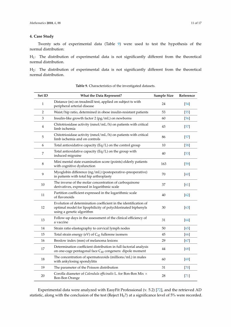
Table 9. Characteristics of the investigated datasets.

Set ID What the Data Represent? Sample Size Reference

1 Distance (m) on treadmill test, applied on subject ts withperipheral arterial disease 24 [54]

2 Waist/hip ratio, determined in obese insulin-resistant patients 53 [55]

3 Insulin-like growth factor 2 (pg/mL) on newborns 60 [56]

4 Chitotriosidase activity (nmol/mL/h) on patients with criticallimb ischemia 43 [57]

5 Chitotriosidase activity (nmol/mL/h) on patients with criticallimb ischemia and on controls 86 [57]

6 Total antioxidative capacity (Eq/L) on the control group 10 [58]

7 Total antioxidative capacity (Eq/L) on the group withinduced migraine 40 [53]

8 Mini mental state examination score (points) elderly patientswith cognitive dysfunction 163 [59]

9 Myoglobin difference (ng/mL) (postoperative–preoperative)in patients with total hip arthroplasty 70 [60]

10 The inverse of the molar concentration of carboquinonederivatives, expressed in logarithmic scale 37 [61]

11 Partition coefficient expressed in the logarithmic scaleof flavonoids 40 [62]

12Evolution of determination coefficient in the identification ofoptimal model for lipophilicity of polychlorinated biphenylsusing a genetic algorithm

30 [63]

13 Follow-up days in the assessment of the clinical efficiency ofa vaccine 31 [64]

14 Strain ratio elastography to cervical lymph nodes 50 [65]

15 Total strain energy (eV) of C42 fullerene isomers 45 [66]

16 Breslow index (mm) of melanoma lesions 29 [67]

17 Determination coefficient distribution in full factorial analysison one-cage pentagonal face C40 congeners: dipole moment 44 [68]

18 The concentration of spermatozoids (millions/mL) in maleswith ankylosing spondylitis 60 [69]

19 The parameter of the Poisson distribution 31 [70]

20 Corolla diameter of Calendula officinalis L. for Bon-Bon Mix ×Bon-Bon Orange 28 [71]

Experimental data were analyzed with EasyFit Professional (v. 5.2) [72], and the retrieved ADstatistic, along with the conclusion of the test (Reject H0?) at a significance level of 5% were recorded.

Mathematics 2018, 6, 88 12 of 17

The AD statistic and the sample size for each dataset were used to retrieve the p-value calculated withour method. As a control method, the formulas presented in Table 3 [43], implemented in an Excel file(SPC for Excel) [47], were used. The obtained results are presented in Table 10.

Table 10. Anderson–Darling (AD) statistic, associated p-values, and test conclusion: comparisons.

SetEasyFit Our Method SPC for Excel

AD Statistic Reject H0? p-Value Reject H0? p-Value Reject H0?

1 1.18 No 0.2730 No 0.0035 Yes2 1.34 No 0.2198 No 0.0016 Yes3 15.83 Yes 3.81 × 10−8 Yes 0.0000 Yes4 1.59 No 0.1566 No 4.63 × 10−15 Yes5 6.71 Yes 0.0005 Yes 1.44 × 10−16 Yes6 0.18 No o.o.r. 0.8857 No7 3.71 Yes 0.0122 Yes 1.93 × 10−9 Yes8 11.70 Yes 2.49 × 10−6 Yes 3.45 × 10−28 Yes9 0.82 No 0.4658 No 0.0322 Yes

10 0.60 No 0.6583 No 0.1109 No11 0.81 No 0.4752 No 0.0334 Yes12 0.34 No o.o.r. 0.4814 No13 4.64 Yes 0.0044 Yes 0.0000 Yes14 1.90 No 0.1051 No 0.0001 Yes15 0.39 No 0.9297 No 0.3732 No16 0.67 No 0.5863 No 0.0666 No17 5.33 Yes 0.0020 Yes 2.23 × 10−13 Yes18 2.25 No 0.0677 No 9.18 × 10−6 Yes19 1.30 No 0.2333 No 0.0019 Yes20 0.58 No 0.6774 No 0.1170 No

AD = Anderson–Darling; o.o.r = out of range.

A perfect concordance was observed in regard to the statistical conclusion regarding the normaldistribution, when our method was compared to the judgment retrieved by EasyFit. The concordanceof the results between SPC and EasyFit, respectively, with the proposed method, was 60%, withdiscordant results for both small (e.g., n = 24, set 1) samples as well as high (e.g., n = 70, set 9) samplesizes. Normal probability plots (P–P) and the quantile–quantile plots (Q–Q) of these sets show slight,but not significant deviations from the expected normal distribution (Figure 6).

Without any exceptions, the p-values calculated by our implemented method had higher valuescompared to the p-values achieved by SPC for Excel. The most substantial difference is observed forthe largest dataset (set 8), while the smallest difference is noted for the set with 45 experimental datavalues (set 15). The lowest p-value was obtained by the implemented method for set 3 (see Table 10);the SPC for Excel retrieves, for this dataset, a value of 0.0000. The next smallest p-value was observedfor set 8. For both these sets, an agreement related to the statistical decision was found (see Table 10).

Our team has previously investigated the effect of sample size on the probability ofAnderson–Darling test, and the results are published online at http://l.academicdirect.org/Statistics/tests/AD/. The method proposed in this manuscript, as compared to the previous one, assures ahigher resolution expressed by the lower unexplained variance between the AD and the model using aformula with a smaller number of coefficients. Furthermore, the unexplained variance of the methodpresent in this manuscript has much less weight for big “p-values”, and much higher weight for small“p-values”, which means that is more appropriate to be used for low (e.g., p ~10−5) and very low(p ~10−10) probabilities.

Mathematics 2018, 6, 88 13 of 17Mathematics 2018, 6, x FOR PEER REVIEW   12 of 12 

-2

-1

0

1

2

3E

xpe

cte

d N

orm

al V

alu

e

 

0.01 0.05 0.25 0.50 0.75 0.90

150

200

250

300

350

400

450

500

550

Ob

serv

ed

va

lue

- s

et

9

 

-1.5

-1.0

-0.5

0.0

0.5

1.0

1.5

2.0

2.5

Exp

ect

ed

No

rma

l Va

lue

 

0.01 0.05 0.10 0.25 0.50 0.75 0.90

1.8

2.0

2.2

2.4

2.6

2.8

3.0

3.2

3.4

3.6

3.8

4.0

Ob

serv

ed

va

lue

- s

et

11

 

Figure 6. Normal probability plots (P–P) and quantile‐quantile plot (Q–Q) by example: graphs for set 

9 (n = 70) in the first row, and for set 11 (n = 40) in the second row. 

Our team has previously investigated the effect of sample size on the probability of Anderson–

Darling test, and the results are published online at http://l.academicdirect.org/Statistics/tests/AD/. 

The method  proposed  in  this manuscript,  as  compared  to  the  previous  one,  assures  a  higher 

resolution  expressed by  the  lower unexplained variance between  the AD and  the model using a 

formula with a smaller number of coefficients. Furthermore, the unexplained variance of the method 

present in this manuscript has much less weight for big “p‐values”, and much higher weight for small 

“p‐values”, which means that is more appropriate to be used for low (e.g., p ~10−5) and very low (p 

~10−10) probabilities. 

Further research could be done in both the extension of the proposed method and the evaluation 

of its performances. The performances of the reported method could be evaluated for the whole range 

of  sample  sizes  if  proper  computational  resources  exist.  Furthermore,  the  performance  of  the 

implementation could be assessed using game  theory and game experiments  [73,74] using or not 

using diagnostic metrics  (such as validation, confusion matrices, ROC analysis, analysis of errors, 

etc.) [75,76]. 

The implemented method provides a solution to the calculation of the p‐values associated with 

Anderson–Darling statistics, giving proper weight to the sample size of the investigated experimental 

data.  The  advantage  of  the  proposed  estimation method,  Equation  (5),  is  its  very  low  residual 

(unexplained variance) and its very high estimation accuracy at convergence (with increasing of in 

and for p near 1). The main disadvantage is related to its out of range p‐values for small AD values, 

but an extensive simulation study could solve this issue. The worst performances of the implemented 

methods are observed when simultaneously n is very low (2 or 3) and p is near 0.5 (50–50%). 

Author Contributions: L.J. and S.D.B. conceived and designed the experiments; L.J. performed the experiments; 

L.J. and S.D.B. analyzed the data; S.D.B. wrote the paper and L.J. critically reviewed the manuscript. 

Acknowledgments: No grants have been received in support of the research work reported in this manuscript. 

No funds were received for covering the costs to publish in open access. 

Figure 6. Normal probability plots (P–P) and quantile-quantile plot (Q–Q) by example: graphs for set 9(n = 70) in the first row, and for set 11 (n = 40) in the second row.

Further research could be done in both the extension of the proposed method and the evaluationof its performances. The performances of the reported method could be evaluated for the wholerange of sample sizes if proper computational resources exist. Furthermore, the performance of theimplementation could be assessed using game theory and game experiments [73,74] using or notusing diagnostic metrics (such as validation, confusion matrices, ROC analysis, analysis of errors,etc.) [75,76].

The implemented method provides a solution to the calculation of the p-values associated withAnderson–Darling statistics, giving proper weight to the sample size of the investigated experimentaldata. The advantage of the proposed estimation method, Equation (5), is its very low residual(unexplained variance) and its very high estimation accuracy at convergence (with increasing of inand for p near 1). The main disadvantage is related to its out of range p-values for small AD values,but an extensive simulation study could solve this issue. The worst performances of the implementedmethods are observed when simultaneously n is very low (2 or 3) and p is near 0.5 (50–50%).

Author Contributions: L.J. and S.D.B. conceived and designed the experiments; L.J. performed the experiments;L.J. and S.D.B. analyzed the data; S.D.B. wrote the paper and L.J. critically reviewed the manuscript.

Acknowledgments: No grants have been received in support of the research work reported in this manuscript.No funds were received for covering the costs to publish in open access.

Conflicts of Interest: The authors declare no conflict of interest.

Mathematics 2018, 6, 88 14 of 17

References

1. Nimon, K.F. Statistical assumptions of substantive analyses across the General Linear model: A Mini-Review.Front. Psychol. 2012, 3, 322. [CrossRef] [PubMed]

2. Hoekstra, R.; Kiers, H.A.; Johnson, A. Are assumptions of well-known statistical techniques checked, andwhy (not)? Front. Psychol. 2012, 3, 137. [CrossRef] [PubMed]

3. Kolmogorov, A. Sulla determinazione empirica di una legge di distribuzione. Giornale dell’Istituto Italianodegli Attuari 1933, 4, 83–91.

4. Smirnov, N. Table for estimating the goodness of fit of empirical distributions. Ann. Math. Stat. 1948, 19,279–281. [CrossRef]

5. Anderson, T.W.; Darling, D.A. Asymptotic theory of certain “goodness-of-fit” criteria based on stochasticprocesses. Ann. Math. Stat. 1952, 23, 193–212. [CrossRef]

6. Anderson, T.W.; Darling, D.A. A Test of Goodness-of-Fit. J. Am. Stat. Assoc. 1954, 49, 765–769. [CrossRef]7. Pearson, K. Contribution to the mathematical theory of evolution. II. Skew variation in homogenous material.

Philos. Trans. R. Soc. Lond. 1895, 91, 343–414. [CrossRef]8. Cramér, H. On the composition of elementary errors. Scand. Actuar. J. 1928, 1, 13–74. [CrossRef]9. Von Mises, R.E. Wahrscheinlichkeit, Statistik und Wahrheit; Julius Springer: Berlin, Germany, 1928.10. Shapiro, S.S.; Wilk, M.B. An analysis of variance test for normality (complete samples). Biometrika 1965, 52,

591–611. [CrossRef]11. Jarque, C.M.; Bera, A.K. Efficient tests for normality, homoscedasticity and serial independence of regression

residuals. Econ. Lett. 1980, 6, 255–259. [CrossRef]12. Jarque, C.M.; Bera, A.K. Efficient tests for normality, homoscedasticity and serial independence of regression

residuals: Monte Carlo evidence. Econ. Lett. 1981, 7, 313–318. [CrossRef]13. Jarque, C.M.; Bera, A.K. A test for normality of observations and regression residuals. Int. Stat. Rev. 1987, 55,

163–172. [CrossRef]14. D’Agostino, R.B.; Belanger, A.; D’Agostino, R.B., Jr. A suggestion for using powerful and informative tests of

normality. Am. Stat. 1990, 44, 316–321. [CrossRef]15. Lilliefors, H.W. On the Kolmogorov-Smirnov test for normality with mean and variance unknown. J. Am.

Stat. Assoc. 1967, 62, 399–402. [CrossRef]16. Van Soest, J. Some experimental results concerning tests of normality. Stat. Neerl. 1967, 21, 91–97. [CrossRef]17. Jänstchi, L.; Bolboacă, S.D. Performances of Shannon’s entropy statistic in assessment of distribution of data.

Ovidius Univ. Ann. Chem. 2017, 28, 30–42. [CrossRef]18. Noughabi, H.A. Two Powerful Tests for Normality. Ann. Data Sci. 2016, 3, 225–234. [CrossRef]19. Zamanzade, E.; Arghami, N.R. Testing normality based on new entropy estimators. J. Stat. Comput. Simul.

2012, 82, 1701–1713. [CrossRef]20. Peng, H.; Tan, F. Jackknife empirical likelihood goodness-of-fit tests for U-statistics based general estimating

equations. Bernoulli 2018, 24, 449–464. [CrossRef]21. Shah, R.D.; Bühlmann, P. Goodness-of-fit tests for high dimensional linear models. Journal of the Royal

Statistical Society. Ser. B Stat. Methodol. 2018, 80, 113–135. [CrossRef]22. Balakrishnan, K.; Sooriyarachchi, M.R. A goodness of fit test for multilevel survival data. Commun. Stat.

Simul. Comput. 2018, 47, 30–47. [CrossRef]23. Perera, A.A.P.N.M.; Sooriyarachchi, M.R.; Wickramasuriya, S.L. A Goodness of Fit Test for the Multilevel

Logistic Model. Commun. Stat. Simul. Comput. 2016, 45, 643–659. [CrossRef]24. Villaseñor, J.A.; González-Estrada, E.; Ochoa, A. On Testing the inverse Gaussian distribution hypothesis.

Sankhya B 2017. [CrossRef]25. MacKenzie, D.W. Applying the Anderson-Darling test to suicide clusters: Evidence of contagion at U. S.

Universities? Crisis 2013, 34, 434–437. [CrossRef] [PubMed]26. Müller, C.; Kloft, H. Parameter estimation with the Anderson-Darling test on experiments on glass. Stahlbau

2015, 84, 229–240. [CrossRef]27. Içen, D.; Bacanlı, S. Hypothesis testing for the mean of inverse Gaussian distribution using α-cuts. Soft

Comput. 2015, 19, 113–119. [CrossRef]28. Ghasemi, A.; Zahediasl, S. Normality tests for statistical analysis: A guide for non-statisticians. Int. J.

Endocrinol. Metab. 2012, 10, 486–489. [CrossRef] [PubMed]

Mathematics 2018, 6, 88 15 of 17

29. Hwe, E.K.; Mohd Yusoh, Z.I. Validation guideline for small scale dataset classification result in medicaldomain. Adv. Intell. Syst. Comput. 2018, 734, 272–281. [CrossRef]

30. Ruxton, G.D.; Wilkinson, D.M.; Neuhäuser, M. Advice on testing the null hypothesis that a sample is drawnfrom a normal distribution. Anim. Behav. 2015, 107, 249–252. [CrossRef]

31. Lang, T.A.; Altman, D.G. Basic statistical reporting for articles published in biomedical journals: The“Statistical Analyses and Methods in the Published Literature” or The SAMPL Guidelines. In Science Editors’Handbook; European Association of Science Editors, Smart, P., Maisonneuve, H., Polderman, A., Eds.; EASE:Paris, France, 2013; Available online: http://www.equator-network.org/wp-content/uploads/2013/07/SAMPL-Guidelines-6-27-13.pdf (accessed on 3 January 2018).

32. Curran-Everett, D.; Benos, D.J. American Physiological Society. Guidelines for reporting statistics in journalspublished by the American Physiological Society.

33. Curran-Everett, D.; Benos, D.J. Guidelines for reporting statistics in journals published by the AmericanPhysiological Society: The sequel. Adv. Physiol. Educ. 2007, 31, 295–298. [CrossRef] [PubMed]

34. Razali, N.M.; Wah, Y.B. Power comparison of Shapiro-Wilk, Kolmogorov-Smirnov, Lilliefors andAnderson-Darling tests. J. Stat. Model. Anal. 2011, 2, 21–33.

35. Tui, I. Normality Testing—A New Direction. Int. J. Bus. Soc. Sci. 2011, 2, 115–118.36. Saculinggan, M.; Balase, E.A. Empirical Power Comparison of Goodness of Fit Tests for Normality in the

Presence of Outliers. J. Phys. Conf. Ser. 2013, 435, 012041. [CrossRef]37. Sánchez-Espigares, J.A.; Grima, P.; Marco-Almagro, L. Visualizing type II error in normality tests.

Am. Stat. 2017. [CrossRef]38. Yap, B.W.; Sim, S.H. Comparisons of various types of normality tests. J. Stat. Comput. Simul. 2011, 81,

2141–2155. [CrossRef]39. Patrício, M.; Ferreira, F.; Oliveiros, B.; Caramelo, F. Comparing the performance of normality tests with ROC

analysis and confidence intervals. Commun. Stat. Simul. Comput. 2017, 46, 7535–7551. [CrossRef]40. Mbah, A.K.; Paothong, A. Shapiro-Francia test compared to other normality test using expected p-value.

J. Stat. Comput. Simul. 2015, 85, 3002–3016. [CrossRef]41. Arshad, M.; Rasool, M.T.; Ahmad, M.I. Anderson Darling and Modified Anderson Darling Tests for

Generalized Pareto Distribution. Pak. J. Appl. Sci. 2003, 3, 85–88.42. Stephens, M.A. Goodness of fit for the extreme value distribution. Biometrika 1977, 64, 585–588. [CrossRef]43. D’Agostino, R.B.; Stephens, M.A. Goodness-of-Fit Techniques; Marcel-Dekker: New York, NY, USA, 1986;

pp. 123, 146.44. Shin, H.; Jung, Y.; Jeong, C.; Heo, J.-H. Assessment of modified Anderson–Darling test statistics for the

generalized extreme value and generalized logistic distributions. Stoch. Environ. Res. Risk Assess. 2012, 26,105–114. [CrossRef]

45. De Micheaux, P.L.; Tran, V.A. PoweR: A Reproducible Research Tool to Ease Monte Carlo Power SimulationStudies for Goodness-of-fit Tests in R. J. Stat. Softw. 2016, 69. Available online: https://www.jstatsoft.org/article/view/v069i03 (accessed on 10 April 2018).

46. 6ixSigma.org—Anderson Darling Test. Available online: http://6ixsigma.org/SharedFiles/Download.aspx?pageid=14&mid=35&fileid=147 (accessed on 2 June 2017).

47. Spcforexcel. Anderson-Darling Test for Normality. 2011. Available online: http://www.spcforexcel.com/knowledge/basic-statistics/anderson-darling-test-for-normality (accessed on 2 June 2017).

48. Qimacros—Data Normality Tests Using p and Critical Values in QI Macros. © 2015 KnowWare InternationalInc. Available online: http://www.qimacros.com/hypothesis-testing//data-normality-test/#anderson(accessed on 2 June 2017).

49. Jäntschi, L.; Bolboacă, S.D. Distribution Fitting 2. Pearson-Fisher, Kolmogorov-Smirnov, Anderson-Darling,Wilks-Shapiro, Kramer-von-Misses and Jarque-Bera statistics. Bull. Univ. Agric. Sci. Vet. Med. Cluj-NapocaHortic. 2009, 66, 691–697.

50. Mosteller, F. Questions and Answers—Combining independent tests of significance. Am. Stat. 1948, 2, 30–31.[CrossRef]

51. Bolboacă, S.D.; Jäntschi, L.; Sestras, A.F.; Sestras, R.E.; Pamfil, D.C. Pearson-Fisher Chi-Square StatisticRevisited. Information 2011, 2, 528–545. [CrossRef]

52. Rahman, M.; Pearson, L.M.; Heien, H.C. A Modified Anderson-Darling Test for Uniformity. Bull. Malays.Math. Sci. Soc. 2006, 29, 11–16.

Mathematics 2018, 6, 88 16 of 17

53. Matsumoto, M.; Nishimura, T. Mersenne twister: A 623-dimensionally equidistributed uniformpseudo-random number generator (PDF). ACM Trans. Model. Comput. Simul. 1998, 8, 3–30. [CrossRef]

54. Ciocan, A.; Ciocan, R.A.; Gherman, C.D.; Bolboacă, S.D. Evaluation of Patients with Lower ExtremityPeripheral Artery Disease by Walking Tests: A Pilot Study. Not. Sci. Biol. 2017, 9, 473–479. [CrossRef]

55. Răcătăianu, N.; Bolboacă, S.D.; Sitar-Tăut, A.-V.; Marza, S.; Moga, D.; Valea, A.; Ghervan, C. The effect ofMetformin treatment in obese insulin-resistant patients with euthyroid goiter. Acta Clin. Belg. Int. J. Clin.Lab. Med. 2018. [CrossRef] [PubMed]

56. Hăs, măs, anu, M.G.; Baizat, M.; Procopciuc, L.M.; Blaga, L.; Văleanu, M.A.; Drugan, T.C.; Zaharie, G.C.;Bolboacă, S.D. Serum levels and ApaI polymorphism of insulin-like growth factor 2 on intrauterine growthrestriction infants. J. Matern.-Fetal Neonatal Med. 2018, 31, 1470–1476. [CrossRef] [PubMed]

57. Ciocan, R.A.; Drugan, C.; Gherman, C.D.; Cătană, C.-S.; Ciocan, A.; Drugan, T.C.; Bolboacă, S.D. Evaluationof Chitotriosidase as a Marker of Inflammatory Status in Critical Limb Ischemia. Ann. Clin. Lab. Sci. 2017,47, 713–719. [PubMed]

58. Bulboacă, A.E.; Bolboacă, S.D.; Stănescu, I.C.; Sfrângeu, C.-A.; Bulboacă, A.C. Preemptive Analgesic andAnti-Oxidative Effect of Curcumin for Experimental Migraine. BioMed Res. Int. 2017, 2017, 4754701.[CrossRef]

59. Bulboacă, A.E.; Bolboacă, S.D.; Bulboacă, A.C.; Prodan, C.I. Association between low thyroid-stimulatinghormone, posterior cortical atrophy and nitro-oxidative stress in elderly patients with cognitive dysfunction.Arch. Med. Sci. 2017, 13, 1160–1167. [CrossRef] [PubMed]

60. Nistor, D.-V.; Caterev, S.; Bolboacă, S.D.; Cosma, D.; Lucaciu, D.O.G.; Todor, A. Transitioning to the directanterior approach in total hip arthroplasty. Is it a true muscle sparing approach when performed by a lowvolume hip replacement surgeon? Int. Orthopt. 2017, 41, 2245–2252. [CrossRef] [PubMed]

61. Bolboacă, S.D.; Jäntschi, L. Comparison of QSAR Performances on Carboquinone Derivatives. Sci. World J.2009, 9, 1148–1166. [CrossRef] [PubMed]

62. Harsa, A.M.; Harsa, T.E.; Bolboacă, S.D.; Diudea, M.V. QSAR in Flavonoids by Similarity Cluster Prediction.Curr. Comput.-Aided Drug Des. 2014, 10, 115–128. [CrossRef] [PubMed]

63. Jäntschi, L.; Bolboacă, S.D.; Sestras, R.E. A Study of Genetic Algorithm Evolution on the Lipophilicity ofPolychlorinated Biphenyls. Chem. Biodivers. 2010, 7, 1978–1989. [CrossRef] [PubMed]

64. Chirilă, M.; Bolboacă, S.D. Clinical efficiency of quadrivalent HPV (types 6/11/16/18) vaccine in patientswith recurrent respiratory papillomatosis. Eur. Arch. Oto-Rhino-Laryngol. 2014, 271, 1135–1142. [CrossRef][PubMed]

65. Lenghel, L.M.; Botar-Jid, C.; Bolboacă, S.D.; Ciortea, C.; Vasilescu, D.; Băciut, , G.; Dudea, S.M. Comparativestudy of three sonoelastographic scores for differentiation between benign and malignant cervical lymphnodes. Eur. J. Radiol. 2015, 84, 1075–1082. [CrossRef] [PubMed]

66. Bolboacă, S.D.; Jäntschi, L. Nano-quantitative structure-property relationship modeling on C42 fullereneisomers. J. Chem. 2016, 2016, 1791756. [CrossRef]

67. Botar-Jid, C.; Cosgarea, R.; Bolboacă, S.D.; S, enilă, S.; Lenghel, M.L.; Rogojan, L.; Dudea, S.M. Assessmentof Cutaneous Melanoma by Use of Very- High-Frequency Ultrasound and Real-Time Elastography.Am. J. Roentgenol. 2016, 206, 699–704. [CrossRef] [PubMed]

68. Jäntschi, L.; Balint, D.; Pruteanu, L.L.; Bolboacă, S.D. Elemental factorial study on one-cage pentagonal facenanostructure congeners. Mater. Discov. 2016, 5, 14–21. [CrossRef]

69. Micu, M.C.; Micu, R.; Surd, S.; Girlovanu, M.; Bolboacă, S.D.; Ostensen, M. TNF-a inhibitors do not impairsperm quality in males with ankylosing spondylitis after short-term or long-term treatment. Rheumatology2014, 53, 1250–1255. [CrossRef] [PubMed]

70. Sestras, R.E.; Jäntschi, L.; Bolboacă, S.D. Poisson Parameters of Antimicrobial Activity: A QuantitativeStructure-Activity Approach. Int. J. Mol. Sci. 2012, 13, 5207–5229. [CrossRef] [PubMed]

71. Bolboacă, S.D.; Jäntschi, L.; Baciu, A.D.; Sestras, R.E. Griffing’s Experimental Method II: Step-By-StepDescriptive and Inferential Analysis of Variances. JP J. Biostat. 2011, 6, 31–52.

72. EasyFit. MathWave Technologies. Available online: http://www.mathwave.com (accessed on 25 March2018).

73. Arena, P.; Fazzino, S.; Fortuna, L.; Maniscalco, P. Game theory and non-linear dynamics: The ParrondoParadox case study. Chaos Solitons Fractals 2003, 17, 545–555. [CrossRef]

Mathematics 2018, 6, 88 17 of 17

74. Ergün, S.; Aydogan, T.; Alparslan Gök, S.Z. A Study on Performance Evaluation of Some Routing AlgorithmsModeled by Game Theory Approach. AKU J. Sci. Eng. 2016, 16, 170–176.

75. Hossin, M.; Sulaiman, M.N. A review on evaluation metrics for data classification evaluations. Int. J. DataMin. Knowl. Manag. Process 2015, 5, 1–11. [CrossRef]

76. Gopalakrishna, A.K.; Ozcelebi, T.; Liotta, A.; Lukkien, J.J. Relevance as a Metric for Evaluating MachineLearning Algorithms. In Machine Learning and Data Mining in Pattern Recognition; Perner, P., Ed.; LectureNotes in Computer Science; Springer: Berlin/Heidelberg, Germany, 2013; Volume 7988.

© 2018 by the authors. Licensee MDPI, Basel, Switzerland. This article is an open accessarticle distributed under the terms and conditions of the Creative Commons Attribution(CC BY) license (http://creativecommons.org/licenses/by/4.0/).