computation and approximation of the length scales of

Computation and approximation of the length scales

of harmonic modes with application to the mapping

of surface currents in the Gulf of Eilat

F. Lekien1 and H. Gildor2

Received 17 January 2008; revised 9 January 2009; accepted 28 January 2009; published 26 June 2009.

[1] Open-boundary modal analysis (OMA) is a generalized Fourier transform thatinterpolates, extrapolates, and filters scattered current measurements and produces smoothcurrent maps in coastal areas. Boundary conditions are enforced by adjusting the OMAmodes to the coastline. Filtering is achieved by discarding OMA modes whose lengthscales are below a selected threshold. In this paper, we determine the length scale of theOMA modes, and we derive approximated formulas. Operational use of the OMA modesand the length scale formulas are illustrated on surface currents measured by high-frequency radar in the Gulf of Eilat (Gulf of Aqaba).

Citation: Lekien, F., and H. Gildor (2009), Computation and approximation of the length scales of harmonic modes with application

to the mapping of surface currents in the Gulf of Eilat, J. Geophys. Res., 114, C06024, doi:10.1029/2008JC004742.

1. Introduction

[2] Increasingly accurate remote sensing techniques areavailable for measuring surface currents in coastal areas[Barrick et al., 1985; Gurgel et al., 1999b]. High-frequency(HF) radar stations measuring surface currents, such as theSeaSonde [Hodgins, 1994] or WERA [Gurgel et al., 1999a]flourish along shorelines worldwide. On the basis of Braggresonance from ocean waves and the Doppler shift in thereflected signal, the HF radar station is able to determinethe magnitude of the surface current along a radial joiningthe antenna and any target point [Barrick et al., 1977]. For agiven location, measured radial currents (henceforth ‘‘radi-als’’) from at least two different angles are needed toevaluate directly the surface velocity vector (henceforth‘‘total’’).[3] Figure 1 describes the setting in the Gulf of Eilat in

the northern Red Sea. Two 42 MHz SeaSonde HF radarsystems measure the currents at a spatial resolution ofapproximately 300 m and a temporal resolution of 30 min.There is one SeaSonde at the InterUniversity Institute inEilat (IUI) and another station at the Port of Eilat (PORT).The distance between the two stations is approximately5 km. In order to approximate the current vector at a certainpoint, we need to have radials measurements from bothstations and the two should observe this patch of water fromdifferent angles. Ideally, we want an angle of about 90�between the two radials and, in any case, at least 15�[Barrick, 2002].

[4] In addition to geometric considerations, such as thedistance from the radar stations and the angle between theradials, the accuracy of the measurement is also subject tosea conditions and radio frequency noise levels. As a result,the output of such a sensing system is a time varying cloudof radial measurements. Not only are the radial currentschanging over time but also their number, locations andaccuracy.[5] For practical purposes such as tracking algae blooms

[Olascoaga et al., 2006] or maximizing the dispersion ofpollutants [Lekien et al., 2005], it is necessary to fill thegaps in the data and to control its quality. Several methodsare available to interpolate and extrapolate the radar data:one may perform objective mapping [Kim et al., 2007], useempirical orthogonal functions (EOF) or use Fourier trans-forms. An invaluable advantage of the latter is that thecurrents are written as a sequence of modes, each of whichwith a specific length scale. Filtering can therefore beperformed by thresholding the wavelength of the modes.[6] A disadvantage of the standard Fourier transform is its

inadequacy in coastal areas. Indeed, currents developed in aFourier basis will not necessarily be tangent to a coastline.While this may not be a significant problem in Eulerianstudies, any method based on Lagrangian paths suffersdramatically from such a violation of the boundary con-ditions [Coulliette et al., 2007]. Whether one integratessingle particle paths, computes finite-time stretching, orextracts Lagrangian coherent structures, it is critical to startfrom surface currents that are tangent to the coastline andthat will not allow particle trajectories to penetrate thecoastline.[7] The work of Lynch [1989] and Eremeev et al. [1992a,

1992b] generalizes the notion of Fourier modes to a coastaldomain with an arbitrary coastline. Instead of projecting onproducts of sines and cosines, the modes are defined as theeigenfunctions of the Laplacian for the domain of interest[Lipphardt et al., 2000]. Lekien et al. [2004] show that this

JOURNAL OF GEOPHYSICAL RESEARCH, VOL. 114, C06024, doi:10.1029/2008JC004742, 2009ClickHere

for

FullArticle

1Ecole Polytechnique, Universite Libre de Bruxelles, Brussels,Belgium.

2Department of Environmental Sciences and Energy Research,Weizmann Institute of Science, Rehovot, Israel.

Copyright 2009 by the American Geophysical Union.0148-0227/09/2008JC004742$09.00

C06024 1 of 24

http://dx.doi.org/10.1029/2008JC004742

generalized Fourier basis is complete: it can represent allpossible surface currents and it guarantees that the currentsare tangent to the coastline. Lekien et al. [2004] further adda new sequence of open-boundary modes to allow inflowand outflow through the segments of the boundary that arenot part of the coastline.[8] This procedure is referred to as open-boundary modal

analysis (OMA). Each OMA mode is associated with aspecific wavelength, or length scale. Being able to approx-imate this length scale quickly is essential when performingfiltering or reconstruction of the currents. As shown byLekien and Coulliette [2007], knowledge of accurate lengthscales for OMA modes also provides a premium method forcomputing quasi-turbulent energy spectra.[9] The goal of this study is to derive robust formulas to

compute the length scale of each OMA mode. Indeed, it is anecessary step to enable efficient filtering of the data andaccurate nowcasting. Following Tricoche et al. [2001] andX. Tricoche (Topology simplification for turbulent flowvisualization, paper presented at Grafiktag, Gesellschaftfur Informatik, Saarbrucken, Germany, 2002), we investi-gate the OMA modes and derive their length scale on thebasis of their features. For a given mode, we extract thewidth of the eddies contained in the mode. By eddy, wemean a closed contour of the stream function or the velocitypotential. This ‘‘eddy’’ usually does not correspond to a realeddy in the current field but represents the smallest feature(length scale) of the observed mode. We then derive severalapproximations and compare them with existing formulas(namely, the expressions used by Lipphardt et al. [2000]and Lekien et al. [2004]).[10] Using our approximated formulae for the mode

length scales, we investigate reconstruction of surfacecurrents for the Gulf of Eilat. Because the gulf is a nearlyrectangular basin, with only one segment of open boundary,

it provides an ideal test site for the use of OMA modes, andfor studying the influence of the mode wavelength and thegrid resolution on the mapped currents. The analogy be-tween the Gulf of Eilat and a rectangle enables us todemonstrate the correspondence between the approximatedlength scale formulas developed in this manuscript and thelength scales of the more familiar Fourier modes. Theresults indicate that even in a relatively simple domain, asignificant amount of modes is needed to accurately recon-struct the surface flow (several hundreds of modes at least).

2. Modal Analysis

[11] Following Kaplan and Lekien [2007], we decomposethe two-dimensional velocity field as

v x; tð Þ ¼ r � kyð Þ þ rf;

where y is the stream function, f is the velocity potentialand k is a unit vector orthogonal to the ocean plane. In mostgeophysical flows, a free-slip boundary condition is appliedat the boundary of the domain (i.e., n � v = 0 where n is aunit vector normal to the boundary). We enforce theboundary condition by requiring t � ry = n � rf = 0.Notice that t � ry = 0 implies that y is constant along theboundary. We can therefore assume, without loss ofgenerality, that y = 0 along the boundary.[12] For many flow problems on a rectangle, one can

further represent the stream function as an infinite sequenceof Fourier modes

y x; y; tð Þ ¼X1i;j¼1

aij tð Þ sin ipx

L

� �sin jp

y

W

� �|fflfflfflfflfflfflfflfflfflfflfflfflfflfflfflfflffl{zfflfflfflfflfflfflfflfflfflfflfflfflfflfflfflfflffl}

yij

;

Figure 1. (left) Radial currents on 29 November 2005 at 1000 UT from the stations PORT (purple) andIUI (black). (right) Approximated total vectors are computed in regions where radial coverage in twodistinct directions is available. In order to directly compute the total vector from the radials mea-surements, we need to combine nearby radials from at least two different angles. As a result, there arealways more radial measurements than computed vector components.

C06024 LEKIEN AND GILDOR: LENGTH SCALES OF HARMONIC MODES

2 of 24

C06024

where L and W are the length (longest dimension) and width(shortest dimension) of the rectangular box.[13] Similarly, the velocity potential can be expanded as

f x; y; tð Þ ¼X1i;j¼0

i;jð Þ6¼ 0;0ð Þ

bij tð Þ cos ipx

L

� �cos jp

y

W

� �|fflfflfflfflfflfflfflfflfflfflfflfflfflfflfflfflffl{zfflfflfflfflfflfflfflfflfflfflfflfflfflfflfflfflffl}

fij

:

[14] A valuable property of the Fourier decomposition isthe fact that each term satisfies, independently, the boundarycondition. As a result, one can modify the coefficients aij(t)and bij(t) freely without any impact on the global boundarycondition. Experimental and numerical errors on the coef-ficients aij(t) and bij(t) do not have any effect on the globalboundary condition.[15] Open-boundary modal analysis is a generalized

Fourier transform for domains that are not rectangular.Given a compact domain W and its boundary @W, thegeneralized stream function modes are defined by thefunctional eigenvalue problem with Dirichlet boundaryconditions

Dyn ¼ l2n yn inside W and yn ¼ 0 on @W :

The generalized potential modes are defined as the solutionsof the Neumann eigenvalue problem

Dfn ¼ l2n fn inside W and n�rfn ¼ 0 on @W:

[16] In both cases, we ignore the trivial and constanteigenmodes corresponding to zero eigenvalues. If the do-main W is a rectangle, the definitions above reduce to theFourier modes. They are, however, applicable to anygeometry and they provide free-slip modes also when thedomain is not a rectangle. Standard results in functionalanalysis guarantee that any smooth (or piecewise smooth)stream function y(x, t) vanishing at the boundary @W can bewritten as

y x; tð Þ ¼X1n¼1

an tð Þyn xð Þ:

where yn are the generalized Dirichlet modes. Similarly,any smooth velocity potential whose normal derivativevanishes at the boundary can be written as a linearcombination of the generalized Neumann modes

f x; tð Þ ¼X1n¼1

bn tð Þfn xð Þ:

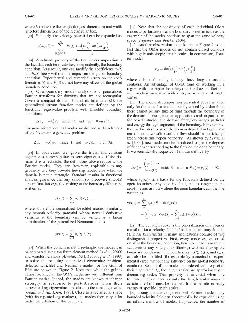
[17] When the domain is not a rectangle, the modes canbe computed using the finite element method [Aubin, 2000]and Arnoldi iterations [Arnoldi, 1951; Lehoucq et al., 1998]to solve the resulting generalized eigenvalue problem.Selected Dirichlet and Neumann modes for the Gulf ofEilat are shown in Figure 2. Note that while the gulf isalmost rectangular, the OMA modes are very different fromFourier modes. Indeed, the modes are known to changestrongly in response to perturbations when theircorresponding eigenvalues are close to the next eigenvalue[Golub and Van Loan, 1996]. Close to a rectangular shape(with its repeated eigenvalues), the modes then vary a lotunder perturbation of the boundary.

[18] Note that the sensitivity of each individual OMAmodes to perturbations of the boundary is not an issue as theensemble of the modes continue to span the same velocityspace [Trefethen and Betcke, 2006].[19] Another observation to make about Figure 2 is the

fact that the OMA modes do not contain closed contourswith highly anisotropic length scales. In comparison, Four-ier modes

yij ¼ sin ipx

L

� �sin jp

y

W

� �;

where i is small and j is large, have long anisotropiccontours. An advantage of OMA (and of working in aregion with a complex boundary) is therefore the fact thateach mode is associated with a very narrow band of lengthscales.[20] The modal decomposition presented above is valid

only for domains that are completely closed by a shoreline;there cannot be any flux of fluid through the boundary ofthe domain. In most practical applications and, in particular,for coastal studies, the domain freely exchanges particlesand energy through segments of the boundary. For example,the southwestern edge of the domain depicted in Figure 2 isnot a material coastline and the flow should let particles gofreely across this ‘‘open boundary.’’ As shown by Lekien etal. [2004], new modes can be introduced to span the degreesof freedom corresponding to the flow on the open boundary.If we consider the sequence of modes defined by

Dfbn ¼

I@Wgn sð Þ ds

Area Wð Þ inside W and n�rfbn ¼ gn sð Þ on @W;

where {gn(s)} is a basis for the functions defined on theopen boundary. Any velocity field, that is tangent to thecoastline and arbitrary along the open boundary, can then bewritten as

v x; tð Þ ¼X1n¼1

an tð Þr � kyn xð Þð Þ

þX1n¼1

bn tð Þrfn xð Þ þX1n¼1

cn tð Þrfbn xð Þ :

[21] The equation above is the generalization of a Fouriertransform for a velocity field defined on an arbitrary domainW. It has been useful in many applications because of twodistinguished properties. First, every mode yn, fn or fn

b

satisfies the boundary condition, hence one can truncate thesequence at any n (e.g., for filtering) without altering theboundary conditions. The coefficients an(t), bn(t), and cn(t)can also be modified (for example by numerical or exper-imental error) without any influence on the global boundarycondition. Second, if the modes are ordered with respect totheir eigenvalue ln, the length scales are approximately indecreasing order. This property is essential when onetruncates the sequence as only the length scales above acertain threshold must be retained. It also permits to studyenergy at specific length scales.[22] Using the above generalized Fourier modes, any

bounded velocity field can, theoretically, be expanded usingan infinite number of modes. In practice, the number of


3 of 24

C06024

available modes is finite and only signals with wavelengthsabove a certain threshold are taken into account. One thenhas to decide what the threshold length scale is and howmany modes are needed to represent the observed velocityfield accurately. This the main subject of this manuscript.

3. Modal Length Scales

[23] In this section, we consider the open-boundarymodes and present several approaches to define their

synoptic length scale. We start from the well-known wave-length of Fourier modes in a rectangular basin. We thenextend the definition to arbitrary OMA modes and wedemonstrate the procedure in a nearly rectangular domain,which enables a clear comparison to the Fourier modes.

3.1. Length Scales of Fourier Modes

[24] Before defining and investigating the length scales ofthe generalized modes defined in the previous section, webriefly review Fourier modes and their length scales. Let usconsider a rectangular box of length L and width W. Without

Figure 2. Selected (top) Dirichlet, (middle) Neumann, and (bottom) boundary modes for the Gulf ofEilat. Circles indicate clockwise vorticity centers (Dirichlet) or point sources (Neumann). Squaresindicate counterclockwise centers (Dirichlet) or sinks (Neumann). Crosses indicate saddle points.


4 of 24

C06024

loss of generality, we assume L � W. The Fourier Dirichletmode

yij ¼ sin ipx

L

� �sin jp

y

W

� �;

delineates Nc = ij identical eddy-like structures. We willrefer to any large closed contour of the stream function as aneddy although it does not necessarily correspond to a realeddy in the current field. Rather than an actual physicalprocess, the eddies in this manuscript represent the atomicfeatures and, hence, the length scales of an observed mode.[25] In the mode yi j, the eddies are arranged in i

columns and j rows. The length scale of the mode can bedefined as the width (or smallest dimension) of the eddies:

lmin¼:min L

i;Wj

n o. This is also the size of the smallest feature

in the mode.[26] One could also think about defining the length

scale as the length (i.e., the largest dimension) of the eddies:

lh ¼: max Li;Wj

n oor the diameter of the eddies: lmax ¼:ffiffiffiffiffiffiffiffiffiffiffiffiffiffi

L2

i2þ W 2

j2

q(i.e., the largest straight segment contained entirely

in a single eddy). Nevertheless, as the arguments below show,only the width or (the size of the smallest feature) is accept-able and physically meaningful.[27] 1. A basic requirement in defining modal length

scales is the ability to order the modes. In particular, theset of modes whose length scale is smaller than a constant Kmust be finite and the number must be increasing with theconstant K. To nowcast currents using OMA, one typicallyputs a threshold on the smallest length scale and projects thedata on the modes whose length scales are larger than thethreshold. This is only possible if there are only a finite numberof modes whose length scale is smaller than the threshold.From this point of view, only lmin is a valid definition.[28] 2. For a mode corresponding to i = 1 and j = 1000,

we have lh = L and lmax � L. One would, however, notattribute such a large length scale to this mode by looking ata plot of its level sets. Indeed, the mode contains very longbut thin eddies whose widths are only H

1000 L. Only lmin is

able to characterize this structure.[29] 3. Two approximations of the length scale have been

proposed in the literature. These approximations will bediscussed in the next section, but we point out already thatthe approximation of Lipphardt et al. [2000], in the contextof Fourier modes, states

lLKG00ij ¼ plij

¼ LWffiffiffiffiffiffiffiffiffiffiffiffiffiffiffiffiffiffiffiffiffiffiffiffii2W 2 þ j2L2

p :

Figure 3. Length scale definitions for Fourier modes. lh isthe length or largest dimension of the eddies; lmax is thediameter of the eddies. These two definitions lead to ametric with which the modes cannot be ordered. l is thesquare root of the area per eddy and does not correspond tothe actual length scale of the mode. lmin is the width of theeddies and a valid, ordering definition of the length scale.Previous length scale approximations [see Lipphardt et al.,2000; Lekien et al., 2004] bracket lmin. Each panelcorresponds to a different aspect ratio: (top) r = L/W = 1,(middle) r = L/W = 2, and (bottom) r = L/W = 5. Note thatthe number of modes below a specific threshold fordefinitions lh, lmax, and l is not necessarily finite.


5 of 24

C06024

The length scale approximation of Lekien et al. [2004] forFourier modes gives

lLCBM04ij ¼ W

l11

lij

¼ffiffiffiffiffiffiffiffiffiffiffiffiffiffiffiffiffiL2 þW 2

pffiffiffiffiffiffiffiffiffiffiffiffiffiffiffiffiffiffiffiffiffiffiffiffii2W 2 þ j2L2

p :

[30] These approximations tell us how the length scalewas defined in the context of operational modal reconstruc-tion. Figure 3 shows the length scales lmin, lh, lmax, and l, as

well as the approximations lijLKG00 and lij

LCBM04. The twoapproximations used previously bracket lmin and are notmeant to represent the quantities lmax or lh.[31] Note that in this paper, the eigenvalues are written

lij2, and not just lij as in the works by Lipphardt et al.

[2000] and Lekien et al. [2004], hence the equations for theapproximated length scales in these papers differ slightlyfrom the equations above.

3.2. Length Scales of Dirichlet Eigenmodes

[32] We now turn to the generalized Fourier modesdefined in section 2. The solution of Dyn = ln

2yn andyn = 0 at the boundary, is a countable set of functionsyn (ordered by increasing eigenvalues ln). Although thesemodes reduce to the Fourier basis for a rectangular domain,themultiple index is irrelevant for a general domainW. This isthe main difficulty in generalizing the length scale definitionto the eigenfunctions: we do not have access to theexact distribution of the eddies in two independent directions(i and j). How can we generalize the definition of the lengthscale lmin to such modes?[33] Let us consider the closed level sets of yn. Courant’s

nodal line theorem states that there is, at most, n closed zerostreamlines [Courant and Hilbert, 1953] and, hence, n eddycenters. Given the mode yn , let us consider the Nc points xk

c

where yn is a local extremum. Figure 2 shows the distribu-tion of the centers xk

c for selected modes. Numerically, wesolve the eigenvalue problems using the finite elementmethod and linear interpolation on the triangular elements.As a result, the numerical modes are piecewise linear andcenters can be easily extracted [Tricoche et al., 2000]. Foreach center xk

c, we consider the quantity

minm¼1��Nc

m6¼k

d xck ; xcm

� �� ;

where d(x1, x2) is the distance between two points in theplane. This quantity gives the shortest distance between xk

c

and its neighbors. It is an approximation of the scale of theeddy of center xk

c. The only discrepancies arise nearthe boundary where the width might extend toward theboundary, i.e., in a direction where there are not anyneighboring centers. For this reason, we define thegeneralized eddy width as

mk ¼ min 2 d xck ; @W� �

; minm¼1��Nc

m 6¼k

d xck ; xcm

� �� 8><>:

9>=>; ; ð1Þ

where d(xkc, @W) is the (shortest) distance between the center

xkc and the boundary @W.[34] The quantities mk give a length scale for each

eddy in the mode yn. We assume that those lengthscales are similar for each eddy within a single modebut there are still several options for defining a singlelength scale from the Nc eddy length scales mk. Weinvestigate the following candidates: (1) Lmin = min

k¼1��Nc

{mk},

(2) Lmax = mink¼1��Nc

{mk}, (3) Lavg = 1Nc

PNc

k¼1

mk, and

(4) Lrms =

ffiffiffiffiffiffiffiffiffiffiffiffiffiffiffiffi1Nc

PNc

k¼1

m2k

s. Note that all the definitions

above reduce to lmin when the domain is a rectangle (and forany aspect ratio). Do these length scales remain close fornonrectangular domains?[35] Figure 4 also reveals that the gap between Lmin and

Lmax vanishes quickly. Note that all the quantities plotted inFigure 4 behave asymptotically as 1/

ffiffiffin

p, according to

Weyl’s law [Weyl, 1950; Courant and Hilbert, 1953].Nevertheless, Figure 4 (bottom) also indicates that therelative difference between Lmax and Lmin remains above30% as n ! +1. In other words, even for a very largemode index, the range of eddy length scales present in themode remains finite. When a rectangular domain is evenslightly perturbed (e.g., in the Gulf of Eilat), the generalizedFourier basis does not only bend the streamlines near theboundary and separate the degenerated eigenvalues. It alsoblurs the spectrum, and eddies with different length scalesstart coexisting within the same generalized mode.[36] Which one of Lmin, Lavg, Lrms, and Lmax should then

be used to define the length scale of a mode?[37] The analysis in the previous section shows that the

width of an eddy, and not its diameter or its length, must beused to define the length scale of an eddy. Extrapolating thisconclusion indicates that the smallest eddy length scale,Lmin, may be the most natural choice for the definition of themode length scale. Indeed, thresholding the length scale in amodal decomposition process requires the ability to excludemodes that contain eddy length scale smaller than thethreshold. Only Lmin could fulfil this requirement.[38] There are, however, two strong arguments against

using Lmin as a length scale definition. First, it is a rathernoisy quantity and it is very sensitive to numerical errors.To derive the graph in Figure 4, the eigenmodes werecomputed on a mesh containing more than 100,000 trian-gular elements. Smaller meshes lead to similar eigenmodesbut the extraction of the centers often leads to spurious orduplicate centers. Since Lmin is given by the smallest eddylength scale, a duplicate center or a spurious center near theboundary can easily decrease Lmin by several orders ofmagnitude. In Figure 4, the curves corresponding to Lmin

and Lmax are much noisier and sensitive to perturbationsthan Lavg and Lrms which are averaged over all the eddies.[39] The second argument against using Lmin as the

definition of the mode length scale is the fact that mosteddies in a mode have a length scale much larger than Lmin.One of the eddies has a width Lmin but most of them havescales closer to Lavg. This can already be deduced fromFigure 4 which indicates clearly that Lavg � Lrms. It is easy


6 of 24

C06024

to check from the definition that we must have Lrms > Lavgand that the variance of the eddy length scale is given by

s2 ¼ 1

Nc

XNc

k¼1

mk Lavg� �2¼ L2rms L2avg:

[40] In other words, the fact that Lrms � Lavg implies thatthe variance s2 is small and that the length scales mk areclustered around their average Lavg. There are some eddieswith a length scale close to Lmin but the vast majority of theeddies in a mode have length scales close to Lavg � Lrms.Figure 5 gives the distribution of the eddy length scales mk

for 3 different modes and corroborates the fact that Lavg �Lrms usually gives a better representation of the mode lengthscale. We also note from Figure 5 that the upper end of the

spectrum is very sparse and that the width of the largesteddy, Lmax, is not a relevant length scale since only one, orvery few, eddies are as broad as Lmax.[41] Since both Lmin and Lavg � Lrms are valid candidates

for the definition of the mode length scale, we will study

Figure 4. Comparison of candidate length scale defini-tions in the Gulf of Eilat. Lmin and Lmax are the length scaleof the smallest and largest eddy, respectively. Lavg and Lrms

are the average and the root means square of the eddy lengthscales for each mode.

Figure 5. Distribution of the eddy length scale mk forDirichlet modes (top) 200, (middle) 275, and (bottom)300 in the Gulf of Eilat. Lmin is the length scale of thesmallest eddy but most of the eddies in a mode have alength scale close to Lavg � Lrms. Very few eddies havescales comparable to the maximum length scale Lmax.


7 of 24

C06024

both quantities in the remaining of the manuscript. Thevarious approximations will be compared to both Lmin andLrms. Note that the latter is so close to Lavg that a thirdcomparison is obsolete.

3.3. Length Scale for Neumann Eigenmodes

[42] Although we have discussed the length scale of onlyDirichlet Fourier modes in section 3.1, the results translatealmost immediately to Neumann Fourier modes. Indeed, thelength scale of

yij ¼ sin ipx

L

� �sin jp

y

W

� �;

is the same as the length scale of

fij ¼ cos ipx

L

� �cos jp

y

W

� �:

Following section 3.1, when i 6¼ 0 6¼ j, the length scale ofboth Neumann and Dirichlet Fourier modes is given by

lmin ¼ minL

i;W

j

� �:

[43] The only difference between Neumann and Dirichletmodes is the domain of the indexes i and j. For Dirichletmodes, both i and j are strictly greater than 0. For Neumannmodes, there are also nondegenerate solutions correspond-ing to either i = 0 or j = 0. Loosely speaking, for a givenrange of length scales, there are always more Neumannmodes than Dirichlet modes. The length scale formula forDirichlet Fourier modes does not accommodate for vanish-ing i and j, but we can generalize the formula as

lmin ¼

minL

i;W

j

� �if i > 0 and j > 0 ;

min L;W

j

� �¼ W

jif i ¼ 0 ;

minL

i;W

� �if j ¼ 0 :

8>>>>>>><>>>>>>>:

The definition above is identical to that of Dirichlet Fouriermodes, except for the modes corresponding to i = 0 and j = 0.When an index vanishes, we compute the length scale withthe other index, but the result cannot exceed the spatialextent of the domain. Note that L � W, hence L � W

j.

[44] Let us now turn to Neumann modes on an arbitrarydomain. The procedure depicted in section 3.2 for Dirichletmodes can be applied to Neumann modes. For Dirichletmodes, mk was, for each center xk

c, the smallest distance toanother center (or twice the distance to the boundary, ifsmaller). For Neumann modes, we seek sinks and sourcesinstead of centers. Unlike centers, some of these sources andsinks will be on the boundary. Taking this into consider-ation, we define the eddy length scale as

mk ¼ minm1��Nc

m 6¼k

d xck ; xcm

� �� ;

where, for Neumann modes, Nc is the number of sourcesand sinks and xk

c is the position of the kth point ofdivergence.[45] Another approach consists of ignoring the sources

and sinks that are on the boundary. In this case, the eddylength scale mk is given by the same formula as for Dirichletmodes (see equation (1)). Numerically, this can be imple-mented by ignoring sources and sinks that are within a smalldistance from the boundary. Note that this approach isconsistent with the free-slip boundary condition whichimplicitly neglects the narrow boundary layer.[46] Similarly, one can count the saddle points of the

Neumann mode (instead of counting the sources and sinks)to determine the length scale (see Figure 2). Index theory[Guckenheimer and Holmes, 1983] guarantees that a saddlewill be found in each closed loop made by the union ofinvariant lines between sources and sinks. Indeed, if weconsider the velocity field rf where f is a velocitypotential mode, there are heteroclinic connections betweensinks and sources. Any closed loop made by the union ofheteroclinic connections can be deformed into a smoothloop that excludes the sinks and sources. The velocityvectors along the loop will rotate clockwise by 360� asthe loop is traveled in a counterclockwise direction. As aresult the loop has index 1 and it must contain at least onesaddle point, which is the only fixed point associated with anegative index.[47] If one counts the saddle points instead of the sources

and sinks, the length scale is still given by equation (1)where Nc becomes the number of saddles and xk

c are thepositions of the saddles.[48] Defining the length scale on the basis of the saddles

in the Neumann modes results in a better mapping betweenNeumann and Dirichlet modes for a rectangular domain.Indeed the centers of

yij ¼ sin ipx

W

� �sin jp

y

H

� �;

correspond exactly to the saddles of

fij ¼ cos ipx

W

� �cos jp

y

H

� �:

[49] On nonrectangular domains, using the saddles of theNeumann modes to define their length scales guaranteesalso that there is no discrepancy between the length scaledefinitions for Neumann and Dirichlet modes. As an exam-ple, Figure 2 shows the modes y1 and f3 which have thesame length scale. The saddle in the Neumann mode playsthe same role as the center in the Dirichlet mode. Indextheory guarantees that except for the first few Neumannmodes in which there might not be any source nor sink inthe interior of the domain, the three approaches above yieldsimilar results. We have implemented the three methods andfound that after the 10th mode, they yield indistinguishableresults. We note, however, that extracting saddle points is amore complicated numerical operation than the computationof sources and sinks (which are extrema of the velocitypotential modes).


8 of 24

C06024

[50] Figure 6 compares the length scale of Neumann andDirichlet modes. Both Lmin and Lrms are investigated. As forDirichlet modes, the ratio between Lmin and Lrms remainsuniformly bounded above 1. Depending on the application,one needs to select one of those two quantities as thereference. It is also worth noting that for a given index n,the length scale of the Neumann mode is always greaterthan the length scale of the Dirichlet mode. Indeed, for agiven length scale threshold, there are always more Neu-mann modes with features larger than the threshold thanthere are Dirichlet modes. On a rectangle, these ‘‘extra’’Neumann modes correspond to pairs of indexes (i, j) whereeither i or j vanishes.[51] Also note that the differences between Neumann and

Dirichlet modes vanish as the mode index, n, increases.Indeed, Figure 6 shows that the quantity Lmin becomes the

same for Neumann and Dirichlet modes as n ! +1. Lrms

has the same asymptotic behavior.

3.4. Length Scale for Boundary Modes

[52] The boundary modes generate flux through segmentsthe of open boundary [Lekien et al., 2004]. They satisfy

Dfbn ¼

I@Wgn sð Þ ds

Area Wð Þ inside W and n � rfbn ¼ gn sð Þ on @W;

where gn(s) is a basis of functions on the open boundary(i.e., where the flux is nonzero). As in the works by Lekienet al. [2004] and Kaplan and Lekien [2007], we assume thata Fourier basis is used for gn. For example, one can use

gn sð Þ ¼ cosnpsLob

� �;

where Lob is the length of the open boundary and n 2 N.[53] As shown by Lekien et al. [2004] and by Kaplan and

Lekien [2007], in this case, the length scale of the nthboundary mode is given by

Lobn ¼ Lob

nþ 1: ð2Þ

[54] Determining the length scale of the boundary modesis therefore a much simpler process than the correspondingoperation for interior Dirichlet and Neumann modes. Theformula above is exact and easily computed for any domainW. In comparison, the ‘‘synoptic length scales’’ Lmin andLrms for interior modes are much more difficult to computeas they require knowledge of the entire mode (as opposed tojust the mode index, n, or the eigenvalue, l) and thecomputation of centers or saddle points.[55] In the next sections, we derive approximations for

the length scale of the interior modes and we compare themto Lmin and Lrms. The objective is to find simple approx-imations that are readily computed (i.e., they depend onlyon n, l, Area(W) and the aspect ratio r) for Dirichlet andNeumann modes. A similar analysis for boundary modes isunnecessary since equation (2) already provides the exactlength scale in terms on n and Lob.[56] Many approximated formulas for an arbitrary domain

will require knowledge of an approximated length (largestdimension of the domain), an approximated width (smallestdimension of the domain) or the aspect ratio (ratio betweenlength and width). In the next section, we derive a meth-odology for determining the width, length, and aspect ratioof an arbitrary domain.

4. Width and Length of an Arbitrary Domain

[57] To derive approximated formula for modal lengthscales, it is often convenient to start from a rectangulardomain where the eigenvalues and the modes are knownanalytically. As a result, and as shown in the next sections,an approximation of the length L of the domain, its widthW,or the aspect ratio r = L/W are often needed to use theseapproximations. These are obvious for a rectangular domain.

Figure 6. Comparison of the synoptic length scales forDirichlet and Neumann modes in the Gulf of Eilat. Lmin isthe length scale of the smallest eddy. Lrms is the root meansquare of the eddy length scales for each mode.


9 of 24

C06024

However, how can we determine the ‘‘largest side’’ Land the aspect ratio of an arbitrary, nonrectangular domainW? In this section, we use the moment of inertia tensor of Wto give a precise definition of L and W for an arbitrarydomain.

4.1. Inertia Tensor

[58] If we consider a bounded open set W � R2, its area is

given by

Area Wð Þ ¼ZZ

Wdx ;

and the center of gravity of the domain is

xg ¼1

Area Wð Þ

ZZWx dx :

[59] Neither the area nor the center of gravity gives anyinformation about the length and the width of the domain.The distribution of the domain about its center of gravity isdetermined by moments of inertia. Suppose that we pick astraight line in the plane that passes through the center ofgravity of W. Such a line is defined by a unit vector wpointing in the direction of the axis. A measure of ‘‘how thedomain is distributed about the axis’’ is given by themoment of inertia

~iw ¼ZZ

Wx xg� �

� w� x xg� ��

dx:

Themomentof inertiacanbecomputed foranyaxisw=(w x,wy)using the moment of inertia along the x and y axes:

~iw ¼ wx wy

� � Ixx IxyIxy Iyy

� �|fflfflfflfflfflfflffl{zfflfflfflfflfflfflffl}

I

wx

wy

� �;

where Ixx = 1x �~ix is the x component of the moment ofinertia with respect to the x axis, and Ixy = 1y �~ix is the ycomponent of the moment of inertia with respect to the xaxis.[60] By definition, we have Ixy = Iyx, hence the 2 � 2

inertia tensor is symmetric. As a result, the matrix I has tworeal eigenvalues corresponding to two orthogonal eigenvec-tors. The norm of the moment of inertia, k~iwk gives ameasure of ‘‘how far the domain extends in the directionperpendicular to w.’’ The direction w is parallel to ‘‘thelargest side’’ of the domain if k~iwk is a minimum. Thedirection w is parallel to ‘‘the smallest side’’ of the domainif k~iwk is maximum. In other words, the distribution of thedomain can be represented by a rectangle whose sides areparallel to the (orthogonal) eigenvectors of the inertiatensor. The eigenvalues of the inertia tensor give the lengthof the sides of the rectangle.

4.2. Length and Width of W[61] The inertia tensor gives us a way to compute a

rectangle that fits the mass distribution inside an arbitrarydomain W. The real eigenvalues lmax and lmin encodeinformation about the size of this rectangle. To extract the

length and width, we seek a rectangle that has an inertiatensor identical to the original domain W. Using a rotationmatrix R that maps the coordinates in the reference frame ofthe eigenvectors of the inertia tensor, we rewrite the inertiatensor as

I ¼ Rlmax 0

0 lmin

� �R>:

[62] The inertia tensor of a rectangle whose sides are Land W and are aligned with the same eigenvectors is givenby

I ¼ 1

3R

L3W 0

0 LW 3

� �R>:

We require that the rectangle used to approximate thedomain has the same area as the original domain W, henceArea(W) = LW and we rewrite the equation above as

I ¼ Area Wð Þ3

RL2 0

0 W 2

� �R>:

For the inertia tensor of the domain W to match that of theapproximating rectangle, we need to set

L ¼:ffiffiffiffiffiffiffiffiffiffiffiffiffiffiffiffiffi3lmax

Area Wð Þ

s;

W ¼:ffiffiffiffiffiffiffiffiffiffiffiffiffiffiffiffiffi3lmin

Area Wð Þ

s:

[63] The formula above gives the length and width of therectangle that has the same center of gravity, the same area,and the same moment of inertia as the domain of interest, W.Given W, it provides a way to compute the length and widthdirectly using the eigenvalues of the moment of inertiatensor. The orientation of the rectangle is given by theeigenvectors of the tensor.[64] It is worth noting that computing the eigenvectors

becomes a singular problem when the eigenvalues areidentical or very close to each other (i.e., when the aspectratio of the domain is close to 1). The largest eigenvalue,which gives the ‘‘largest side of the domain’’ is, however,continuous, independently of the aspect ratio of the domain.In other words, it might be difficult to plot the actualapproximating rectangle when the aspect ratio is close to1, but determining the largest length scale of the domain andits aspect ratio is never a singular problem [Dieci andEirola, 1999].

4.3. Examples

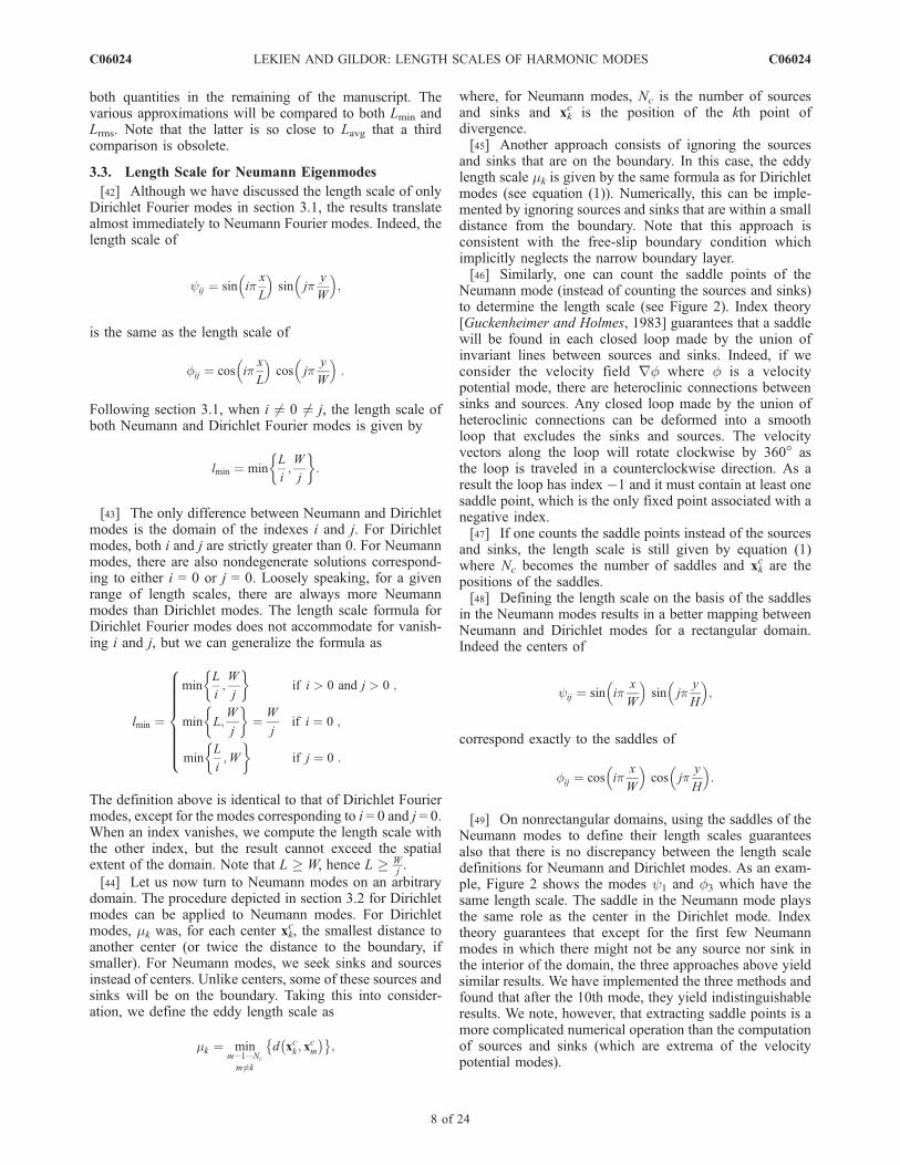
[65] Figure 7 shows the results of two numerical appli-cations: the nearly rectangular basin of the Gulf of Eilat(that we study in this manuscript) and Monterey Bay whichhas a more complex coastline [see, e.g., Paduan andRosenfeld, 1996]. The surface currents in these two regionsare sampled using coastal radar stations. For using some ofthe approximated length scale formula derived in the nextsections and selecting the number of OMA modes to use,one needs to evaluate the ‘‘largest side’’ and the ‘‘smallest


10 of 24

C06024

side’’ of these domains. According to the method describedabove, these lengths are (L, W) = (8.17 km, 6.26 km) for theGulf of Eilat, and (L, W) = (47.6 km, 36.7 km) for MontereyBay. Figure 7 also shows the corresponding approximatedrectangles (dashed rectangles). On both panels, a thick lineindicates the boundary of a computational domain W whereenough data is available for modal analysis. OMA modesand nowcasts are computed for these domains.

5. Approximated Length Scales

[66] Both the smallest eddy width (Lmin) and the averageeddy width (Lrms) are acceptable definitions for the modelength scale. These quantities are, however, difficult to

compute since they require intensive and subtle computa-tions to extract centers and saddles. In this section, weinvestigate several approximations of the length scale andcompare them to Lmin and Lrms.

5.1. A Lower Bound: LLKG00

[67] Let us consider a rectangle and the correspondingFourier eigenvalues

l2ij ¼ p2

i2

L2þ j2

W 2

� �: ð3Þ

For a given l, there might be several couples (i, j) satisfyingthe equation above but we always have

1 � i � L

ffiffiffiffiffiffiffiffiffiffiffiffiffiffiffiffiffiffil2

p2 j2

W 2

s< L

lp; ð4Þ

and

1 � j � W

ffiffiffiffiffiffiffiffiffiffiffiffiffiffiffiffil2

p2 i2

L2

s< W

lp: ð5Þ

The length scale of a Fourier mode is given by

Lmin ¼ minL

i;W

j

� �;

hence we need to treat the couples (i, j) differently on thebasis of the relative magnitude of L/i and W/j. Fromequation (3), we deduce that L/i � W/j if and only if

i � lLffiffiffi2

pp:

In this case, we have

Lmin ¼L

i>

pl;

where we have used the last inequality in (4).[68] Similarly, when L/i > W/j, we find

j >lWffiffiffi2

pp;

and

Lmin ¼W

j>

pl;

by the last inequality in (5).[69] In other words, we have shown that p/l is always

strictly smaller than Lmin for a Dirichlet mode on a rectan-gle. This lower bound was used as an approximation of thelength scale used by Lipphardt et al. [2000], hence wedefine

LLKG00¼: pl;

as a first candidate approximation of Lmin.

Figure 7. Computation of the width and length for the HFradar covered regions in (top) the Gulf of Eilat and (bottom)Monterey Bay. The solid line indicates the computationaldomain where modes and nowcasts are computed. Thedashed line is the rectangle built on the inertia tensor of thedomains that provides width and length for each domain.


11 of 24

C06024

[70] Note that the lower bound is valid for any rectangle;it does not depend on the aspect ratio r = L/W. In general,LLKG00 does not need to remain a lower bound of Lmin whenthe domain is not a rectangle. Nevertheless, as demonstratedin the next section, we expect this quantity to provides anapproximate lower bound of the length scale.[71] The lower bound LLKG00 is valid for both Dirichlet

and Neumann modes. In the case of a Neumann mode,however, the last inequalities in equations (4) and (5) are notstrict and the lower bound is not strict. For some Neumannmodes, Lmin becomes equal to the lower bound LLKG00.

5.2. An Upper Bound: Lup

[72] We have established that when L/i � W/j, we havei � lLffiffi

2p

p. In this case,

Lmin ¼L

i�

ffiffiffi2

p pl:

When L/i > W/j, we have j > lWffiffi2

ppand

Lmin ¼H

j�

ffiffiffi2

p pl:

In both cases, and for any rectangle, we have the upperbound

Lmin �ffiffiffi2

p pl

¼: Lup:

[73] The upper bound Lup is only valid for a rectangulardomain, but we also expect it to overestimate the lengthscale of a mode for a nonrectangular region. Note thatcontrary to the lower bound LLKG00, the upper bound is notstrict. For any rectangle, an infinite number of modes have alength scale equal to Lup.[74] Note that Lipphardt et al. [2006] use the length scale

formula 2pl instead of the formula LLKG00 = p

l from previouswork [Lipphardt et al., 2000]. The quantity 2p

l is always

greater than the upper bound Lup =ffiffiffi2

ppl and is not a good

approximation of the mode length scale in the sensedeveloped here. All the formulas and definition in thismanuscript attempt to define the eddy diameter, or halfthe wavelength of the modes. Indeed, a full period of anoscillating mode has both a minimum and a maximum,hence two eddies. The formulas used by Lipphardt et al.[2006] describe the full wavelength of the modes and,hence, translate into p

l in the context of this study. Similarly,any definition and formulas from this manuscript can bemultiplied by two to obtain results in terms of full wave-lengths.

5.3. A Dimensional Approximation: LLCBM04

[75] In the work by Lekien et al. [2004], an approxima-tion of the modal length scale is derived on the basis ofBuckingham’s P theorem [Buckingham, 1914; Curtis et al.,1982]. If nothing but the eigenvalue (ln

2) is known,Buckingham’s dimensional analysis provides a strong con-straint on the relationship between ln and the length scale,Ln, of the nth mode: their product is a constant that does notdepend on the mode index n. We can therefore find the

length scale of any mode on the basis of a reference mode asfollows

Ln ¼ Lreflref

ln

;

[76] For Dirichlet modes, the reference is naturally thefirst mode [Lekien et al., 2004; Kaplan and Lekien, 2007].Indeed, the first mode corresponds to a single gyre withlength scale L1 = W (e.g., for a rectangle, y11 = sin(px/L)sin(py/W)). As a result, on the basis of Buckingham’s Ptheorem, the length scale of any Dirichlet mode is approx-imated by

Ln ¼ Wl1

ln

;

which is the result given by Lekien et al. [2004].[77] For Neumann modes, using the same formula usually

underestimates the length scale [Kaplan and Lekien, 2007].This is a consequence of the fact that the reference Dirichletmode does not correspond to the first Neumann mode. For arectangle, the first Dirichlet mode is y11. The correspondingNeumann mode (with the same length scale W) is f11 but itis not the first Neumann mode. At least f01 and f10 havesmaller eigenvalues than f11.[78] We can therefore apply Buckingham’s P theorem

also to Neumann modes, provided that we use the correctreference f11. Let us denote by m the index of f11 in the listof Neumann modes ordered by eigenvalues. The lengthscale of the nth Neumann mode is then given by

Ln ¼ Wlm

ln

:

[79] The formula above is not very useful since theindex m of the reference mode is usually unknown. For asquare (L = W), there are only 2 modes with eigenvaluessmaller than that of f11, hence m = 3. When the aspect ratior = L/W > 1, the reference index can be larger than 3. For theGulf of Eilat (r � 1.3), Figure 2 shows that we have m = 3:the third Neumann mode has the same length scale as thefirst Dirichlet mode.[80] Fortunately, one does not need to compute the exact

index m to evaluate the eigenvalue lm and use the formulaabove. Indeed, on a rectangle, we have

l2m ¼ l2

11 ¼ p21

L2þ 1

W 2

� �:

Since we assume L �W, the smallest eigenvalue l1 is givenby

l21 ¼

p2

L2;

hence the approximated Neumann length scale can berewritten

Ln ¼ Wlm

l1

l1

ln

¼ Wffiffiffiffiffiffiffiffiffiffiffiffiffi1þ r2

p l1

ln

;


12 of 24

C06024

where r = L/W is the aspect ratio.The dimensional approximation can then be summarized as

LLCBM04 ¼ nWl1

l; ð6Þ

where n = 1 for Dirichlet modes and n =ffiffiffiffiffiffiffiffiffiffiffiffiffi1þ r2

pfor

Neumann modes.

5.4. An Exact Formula for Fourier Modes: Lrect

[81] For Fourier modes, the number of centers (or sad-dles) inside the domain is given by

Nc ¼ i j:

Since equation (3) gives another equality involving i and j,it is possible to determine i and j from l and Nc. We have

i ¼

ffiffiffiffiffiffiffiffiffiffiffiffiffiffiffiffiffiffiffiffiffiffiffiffiffiffiffiffiffiffiffiffiffiffiffiffiffiffiffiffiffiffiffiffiffiffiffiffiffiffiffiL2l4

2p2� L2

2

ffiffiffiffiffiffiffiffiffiffiffiffiffiffiffiffiffiffiffiffiffiffiffiffiffil2

p4 4

N2c

W 2L2

svuut;

j ¼

ffiffiffiffiffiffiffiffiffiffiffiffiffiffiffiffiffiffiffiffiffiffiffiffiffiffiffiffiffiffiffiffiffiffiffiffiffiffiffiffiffiffiffiffiffiffiffiffiffiffiffiffiffiffiW 2l4

2p2�W 2

2

ffiffiffiffiffiffiffiffiffiffiffiffiffiffiffiffiffiffiffiffiffiffiffiffiffil2

p4 4

N 2c

W 2L2

svuut:

8>>>>>>>><>>>>>>>>:

As a result, we get

Lmin ¼ minL

i;W

j

� �¼

ffiffiffi2

p pl

1þ

ffiffiffiffiffiffiffiffiffiffiffiffiffiffiffiffiffiffiffiffiffiffiffiffiffi1 4p4N2

c

l4W 2L2

s0@

1A

12

:

The formula above gives the exact length scale Lmin for anyFourier mode as a function of its eigenvalue l, the numberof eddy centers Nc, and the area of the domain Area(W) =LW. The formula is only exact for rectangular domains but,for arbitrary regions, we define the candidate approximation

Lrect ¼:ffiffiffi2

p pl

1þ

ffiffiffiffiffiffiffiffiffiffiffiffiffiffiffiffiffiffiffiffiffiffiffiffiffiffiffiffiffiffiffiffi1 4p4N2

c

l4Area2 Wð Þ

s !12

: ð7Þ

Note that for Neumann modes, Nc is the number of saddlepoints, not the number of centers.

5.5. Variants of Lrect

[82] Equation (7) gives the exact length scale when thedomain is a rectangle and is expected to perform very wellon other domains. It does, however, require the computationof Nc, the number of centers (or saddles for Neumannmodes). Since Nc is difficult to compute and is subject toa high numerical error, it is often preferable to approximateNc using the eigenvalue l or the mode index n. We note thefollowing distinguished values for Nc:[83] 1. The first value is Nc

max. On a rectangle, we have

j2 ¼ W 2 l2

p2 i2

L2

� �;

hence,

N2c ¼ i2 j2 ¼ W 2 i2

l2

p2 i4

L2

� �;

which is maximum when i = lWffiffi2

pp. As a result, for a given

eigenvalue l, the maximum value of Nc is

Nmaxc ¼ l2 Area Wð Þ

2p2:

Substituting the expression above in equation (7), we find

Lrectmax¼: ffiffiffi

2p p

l;

which is identical to the upper bound Lup.[84] 2. Similarly, one can determine that the minimum

value for Nc is Ncmin = lH/p. As a result, we have

Lrectmin ¼ffiffiffi2

p pl

1þ

ffiffiffiffiffiffiffiffiffiffiffiffiffiffiffiffiffiffiffiffiffiffiffiffiffiffiffiffiffiffiffiffi1 4p2

l2rArea Wð Þ

s !12

:

The expression above becomes asymptotically (i.e., forl ! +1) identical to the lower bound LLKG00 butimproves the estimate for eigenmodes corresponding tosmall eigenvalues.[85] 3. Since we have both the minimum and maximum

value for Nc, we can also use the average

N avgc ¼ Nmax

c þ Nminc

2¼ l2Area Wð Þ

4p2þ lW

2p:

Substitution in equation (7) gives

Lrectavg¼: pl

2ffiffiffiffiffiffiffiffiffiffiffiffiffiffiffiffiffiffiffiffiffiffiffiffiffiffiffiffiffiffiffiffiffiffiffiffiffiffiffiffiffiffiffiffiffiffiffiffiffiffiffiffiffiffiffiffiffiffiffiffiffiffiffiffiffiffiffiffiffiffiffi2þ

ffiffiffiffiffiffiffiffiffiffiffiffiffiffiffiffiffiffiffiffiffiffiffiffiffiffiffiffiffiffiffiffiffiffiffiffiffiffiffiffiffiffiffiffiffiffiffiffiffiffiffiffiffiffiffiffiffiffi3 4 p2

l2 rArea Wð Þ 4 plffiffiffiffiffiffiffiffiffiffiffiffiffiffirArea Wð Þ

prs :

Notice that as l ! +1, we have

Lrectavg !2ffiffiffiffiffiffiffiffiffiffiffiffiffiffiffi

2þffiffiffi3

pp pl� 1:035

pl;

which is almost identical to LLKG00. As a result, theapproximation Lavg

rect is, asymptotically, very similar to thelower bound LLKG00, but it provides a better estimate forlow eigenvalues for which the lower bound LLKG00 isusually too conservative.[86] 4. Another estimate for Nc can be obtained by

‘‘counting’’ the modes for which the number of centers issmaller than Nc. Recall that we have 1 � i � Nc + 1, and thenumber of modes, n, which have less than Nc centers isapproximately equal to the area under the curve Nc/i in the(i, j) plane. This gives

n �Z Ncþ1

1

Nc

idi ¼ Nc ln Ncþ1ð Þ:

One can check that the function x ln(x + 1) is strictlyincreasing for positive x. As a result, one can compute itsinverse,

Nc ¼ g nð Þ;


13 of 24

C06024

which gives the number of centers (or saddles) as a functionof the mode index n. Notice that the inverse of x ln(x + 1)does not have an analytic expression, hence one needs toevaluate g numerically or build a seek table. Given themode index n, we can then approximate Nc using thetabulated function g, and the expression

Lrectg ¼:ffiffiffi2

p pl

1þ

ffiffiffiffiffiffiffiffiffiffiffiffiffiffiffiffiffiffiffiffiffiffiffiffiffiffiffiffiffiffiffiffiffi1 4p4g2 nð Þ

l4 Area2 Wð Þ

s !12

is an estimate of the length scale of the mode.[87] At first, one would expect the approximation above

to yield poor results as the argument used to derive it isflawed: we have computed the number of modes whichhave less than Nc centers, but this quantity cannot be easilyrelated to the mode index n. Indeed, the mode index n

depends on the position of the mode in a sequence that hasbeen ordered by length scale or by eigenvalue. However, thecomputation above assumes that the index n gives theposition in a sequence ordered by Nc. There is no guaranteethat the ordering by eigenvalue is even close to the orderingby number of centers. In fact, for rectangular domains, onecan show that the two orderings (and the two definitions ofthe mode index n) are very different.[88] As a result, when one evaluates Nc as g(n) where n is

the actual mode index (i.e., ordered by eigenvalue), the errorcan be quite large. Nevertheless, the next section will revealthat only Lavg

rect outperforms Lgrect. We cannot fully explain

this result but, intuitively, the reason is that in a non-rectangular domain, the eigenmodes rearrange in such away that long eddies are replaced by (more numerous)isotropic eddies. Provided that the boundary of the domainis complex enough, most modes tend to be uniformly

Figure 8. Comparison of the synoptic length scales for (top) Dirichlet and (bottom) Neumann modes inthe Gulf of Eilat. Lmin is the length scale of the smallest eddy. Lrms is the root means square of the eddylength scales for each mode. Both Lmin and Lrms can be considered as a synoptic length scale and we seektheir best approximation.


14 of 24

C06024

distributed [Shnirelman, 1974]. For example, on a square,the modes (i, j) = (100, 1) and (i, j) = (1, 100) corresponds toNc = 100, a relatively small number of centers for a largeeigenvalue. The configurations with thin eddies are, how-ever, unstable and any perturbation of the domain willmodify the pair immediately in such a way that the numberof centers is higher in the perturbed modes (see, e.g.,Trefethen and Betcke [2006, Figure 5] for an illustrationof this process on a square with a snipped corner).[89] The accuracy of Lg

rect is therefore not a consequenceof its accuracy for a rectangular domain. It is, in fact lessaccurate than the other approximations for a rectangle.Instead, its strength comes from its ability to model acomplex phenomena that takes place when one deforms arectangular domain into a complex domain W: the modeindex with respect to Nc becomes more and more similar tothe mode index with respect to l as the domain W looks lessand less like a rectangle.

6. Comparison

[90] Figure 8 shows Lmin and Lrms for Dirichlet andNeumann modes in the Gulf of Eilat. Recall that dependingon the application, either Lmin or Lrms could be selected asthe ‘‘true synoptic length scale.’’ Superimposed on each ofthese plots are the approximations developed in the previoussection.[91] We draw the following conclusions:[92] 1. If one uses the average eddy width Lrms as the true

length scale, then the best approximation is LLCBM04. It isworth noting that this conclusion only holds for domainswhose aspect ratio is close to 1.5. For the Gulf of Eilat, thetensor of inertia reveals that the aspect ratio r � 1.3 andLLCBM04 performs well. Inspecting Figure 3 reveals thatLLCBM04 is no longer the best approximation of Lrms whenr � 1 or r > 2. For r � 1, LLCBM04 overestimates the lengthscale. For r > 2, LLCBM04 tends to LLKG00, which under-estimates the length scale. None of our approximations are,however, close to Lrms for r > 2. Lavg

rect is the closest but thereis a significant error. In these cases, we suggest to use theaverage between the upper and lower bounds: 1/2 (Lup + Lmin

rect).[93] 2. If one uses the smallest eddy length scale Lmin as

the truth, then the best approximation is Lrect, which requirescounting the exact number of centers (or saddle points forNeumann modes).[94] 3. If one uses the smallest eddy length scale Lmin as

the truth and does not want to extract features such as cen-ters and saddle points, then the best approximation is Lavg

rect.[95] 4. If one is interested in a lower bound of the

minimum length scale Lmin, the approximation LLKG00 israther conservative (both asymptotically and for smalleigenvalues). At almost no extra computational cost, Lg

rect

and Lminrect provide much better lower bounds on Lmin.

[96] It is worth noting that Lipphardt et al. [2006] used

the approximation LLSK06 = 2pl which is twice the lower

bound LLKG00 = pl. Since LLSK06 = 2p

l >ffiffiffi2

ppl = Lup, the

quantity LLSK06 overestimates the length scale. Figure 8confirms that LLSK06 is not a good approximation of thelength scale (in the context of this manuscript). The formula

LLSK06 = 2pl should be seen as a lower bound for the full

oscillation wavelength (double the eddy length scale). It is

equal to two twice LLKG00 and should be compared to thedouble of the quantities in this manuscript.[97] Note also that the formulas LLKG00, LLSK06 and Lup

have, however, an invaluable advantage: they depend onlyon the eigenvalue l, which is readily available from themode solver. All the other formulas require the computationof the area of the domain, the width W, the aspect ratio r orother less trivial quantities.

7. Nowcasting in the Gulf of Eilat

[98] The northern tip of the Gulf of Eilat is a nearlyrectangular, deep, and semienclosed basin in the northeastregion of the Red Sea. Two 42 MHz HF radar (SeaSonde)stations are installed on the western coast of the gulf, one atthe InterUniversity Institute and the other at the Port of Eilat(separated by approximately 5 km). This network enablesobserving the 6 km � 10 km region at a spatial resolution ofabout 300 m and a temporal resolution of 30 minutes (seeFigure 1). More details on the deployment and validation ofthis network are given by Gildor et al. [2009].[99] To proceed with OMA nowcasting, we begin by

plotting the length scale as a function of the mode indexfor Dirichlet, Neumann, and boundary modes in Figure 9.Using this plot, we can determine the number of modesneeded on the basis of the desired resolution. On the basisof Nyquist criterion, the smallest mode must be larger orequal to the spatial resolution of the data to avoid aliasing.(Note that Nyquist criterion states that the sampling fre-quency must be at least twice the frequency of the signal. Inour case, however, the mode length scale is half the wave-length, hence the factor 2 disappears from the criterion.)One must, however, also ensure that the number of modesused does not exceed the number of radial currents avail-able. This second requirement is usually more constrainingthan Nyquist criterion. For the Gulf of Eilat, it is typicallypossible to assimilate radial data down to a 350 m resolu-tion. Wherever we have two nearby radial measurements,we can directly recombine the radial data into total vectors[Barrick, 2002]. The resulting total vectors count for tworadial measurements and can also be assimilated using theOMA modes. In this case, however, fewer modes can beused since some unpaired radial currents have been dis-carded. It is typically possible to assimilate total currentsdown to a 400 m resolution in the gulf. Because there aremany more radials than totals, it is therefore more advan-tageous to do the OMA nowcasts using radial data [Kaplanand Lekien, 2007]. Another advantage of this procedure isthat it circumvents the errors that result from the way radialsare combined into totals, specifically the Geometric DilutionOf Precision (GDOP [Barrick, 2002; Kim et al., 2008]).Using the radials, we avoid the errors in totals and we usemore data. Note that as a result, the OMA analysis whichassimilates radial data can also be seen as another way tocombine radials into totals. Recently, Kim et al. [2008] pre-sented a generalized optimal interpolation method to com-pute surface currents from radials.[100] We selected 4 different resolution lengths (400 m,

600 m, 1 km, and 2 km) and, using the curves shown inFigure 9, we determined the number of Dirichlet, Neumann,and boundary modes for each case (Table 1). It is worthnoting that the plot in Figure 9 can be easily checked or


15 of 24

C06024

approximated using the closest rectangle. On the basis ofthe method described in section 4, we have determined thata rectangle of 8.17 km by 6.26 km has the same moment ofinertia as the Gulf of Eilat. For the rectangle, one can easilyplot the length scale of the Fourier modes as a function ofthe mode index. Figure 10 compares the length scales forthe modes in the gulf and the Fourier modes. Clearly, thelength scales of the Fourier modes corroborates our com-putations in the gulf and can be used as an approximation ofthe length scale. This conclusion becomes very importantwhen one works with very large sequences of modes. In thiscase, the eigenvalues of the modes and our length scaleapproximation may become imprecise when n ! +1. Thebehavior of the Fourier modes for the closest rectangle can beused to verify the results or to extrapolate the curves for large n.[101] Given a set of Dirichlet modesyi (i = 1 � � � ny), a set of

Neumannmodes fj (j = 1 � � � nf), and a set of boundary modesfkb (k = 1 � � � nb), the nowcast (i.e., the reconstructed velocity

field) is a linear combination of all the modes. The velocity atpoint x is given by

v xð Þ ¼Xnyi¼1

ai r� kyi xð Þð Þ þXnfj¼1

bj rfj xð Þ þXnbk¼1

gk rfbk xð Þ:

ð8Þ

To perform the nowcast, one needs to determine thecoefficients ai, bj, and gk in such a way that the linear

combination best represents the measured radar data. This istypically done by defining a cost function, such as

Ftot ¼XNn¼1

k v xnð Þ vn k2;

where N is the number of total vectors in the radar data, xn isthe position of the nth measurement and vn is the nth totalvector. When assimilating radial measurements (as opposedto total vectors), the data set is a sequence of N radial anglesqn and the corresponding radial currents vn. As depicted byKaplan and Lekien [2007], a cost function for radial dataassimilation is given by

Frad ¼XNn¼1

k 1qn� v xnð Þ vn k2;

where 1qn is the unit vector oriented along the nth radial qn.In both cases the cost function is the difference between thenowcast (reconstructed velocity field which depends on thecoefficients ai, bj and gk) and the observed velocitycomponents. We view this cost as a function of thecoefficients ai, bj and gk and the nowcast is obtained byminimizing the cost function. The corresponding optimalcoefficients ai, bj and gk determine the linear combinationof the selected modes that best fit the data [Lekien et al.,2004].[102] In practice, however, Kaplan and Lekien [2007]

showed that two critical improvements must be brought tothe cost function. First, each term must be weightedinversely proportional to the local measurement density.This modification aims at avoiding the lack of sensitivity ofthe cost function to regions where data collection is sparse.The second major modification is the introduction of asmoothing term which forces the minimum to correspond tocoefficients ai, bj and gk of reasonable magnitude. Indeed,Kaplan and Lekien [2007] showed that without any smooth-ing term, unphysical large coefficients could correspond to

Table 1. Resolution and Number of Modes Used for Current

Reconstruction

Resolution ny nf nb Total Number of Modes (N)

2 km 11 18 5 341 km 46 62 9 117600 m 134 163 14 311400 m 307 354 22 683

Figure 9. Length scale for the Dirichlet, Neumann, andboundary modes in the Gulf of Eilat using the approxima-tion Lavg

rect. By drawing a horizontal line at the desiredresolution on this plot, one determines the number of modesneeded in each sequence of modes.

Figure 10. Comparison of the modal length scales forOMA modes in the Gulf of Eilat and the Fourier modes ofthe rectangle approximating the gulf.


16 of 24

C06024

Figure 11. OMA nowcast on 29 November 2005 at 1000 UT based on radial data. (a–d) Recombinedtotal vectors (red) and reconstructed OMA currents (blue). (e–h) Reconstructed divergence. (i– l) Recon-structed vorticity. The nowcast resolution is 400 m (683 modes) in Figures 11a, 11e, and 11i; 600 m(311 modes) in Figures 11b, 11f, and 11j; 1 km (117 modes) in Figures 11c, 11g, and 11k; and 2 km(34 modes) in Figures 11d, 11h, and 11l.


17 of 24

C06024

Figure 12. OMA nowcast on 29 November 2005 at 1000 UT based on total data. (a–d) Recombinedtotal vectors (red) and reconstructed OMA currents (blue). (e–h) Reconstructed divergence. (i– l) Recon-structed vorticity. The nowcast resolution is 400 m (683 modes) in Figures 12a, 12e, and 12i; 600 m(311 modes) in Figures 12b, 12f, and 12j; 1 km (117 modes) in Figures 12c, 12g, and 12k; and 2 km(34 modes) in Figures 12d, 12h, and 12l.


18 of 24

C06024

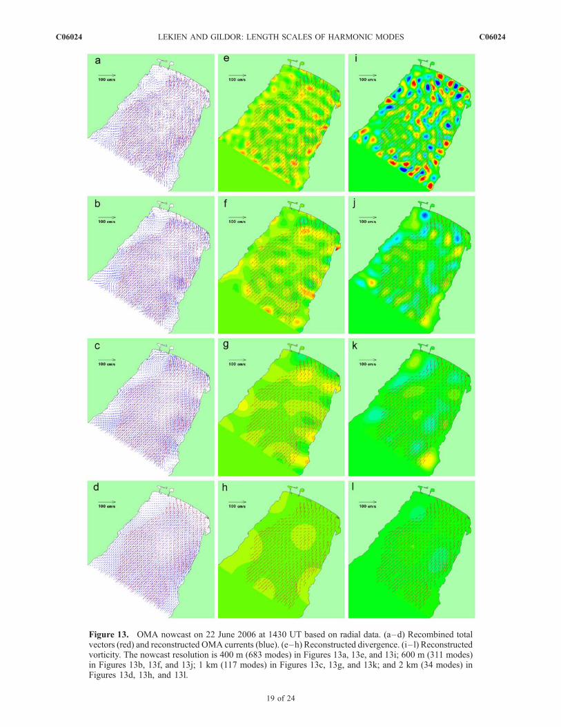
Figure 13. OMA nowcast on 22 June 2006 at 1430 UT based on radial data. (a–d) Recombined totalvectors (red) and reconstructed OMA currents (blue). (e–h) Reconstructed divergence. (i– l) Reconstructedvorticity. The nowcast resolution is 400 m (683 modes) in Figures 13a, 13e, and 13i; 600 m (311 modes)in Figures 13b, 13f, and 13j; 1 km (117 modes) in Figures 13c, 13g, and 13k; and 2 km (34 modes) inFigures 13d, 13h, and 13l.


19 of 24

C06024

Figure 14. OMA nowcast on 22 June 2006 at 1430 UT based on total data. (a–d) Recombined totalvectors (red) and reconstructed OMA currents (blue). (e–h) Reconstructed divergence. (i– l) Reconstructedvorticity. The nowcast resolution is 400 m (683 modes) in Figures 14a, 14e, and 14i; 600 m (311 modes)in Figures 14b, 14f, and 14j; 1 km (117 modes) in Figures 14c, 14g, and 14k; and 2 km (34 modes) inFigures 14d, 14h, and 14l.


20 of 24

C06024

the minimum error for a set of radar measurements. Thesecoefficients lead to unphysical large velocity vectors awayfrom the cloud of measurements. The updated cost functionfor radial measurements is given by

F ¼XNn¼1

1

An|{z}weights

k 1qn� v xnð Þ vn k2

þ KXnyi¼1

a2i þ

Xnfj¼1

b2j þ

Xnbk¼1

g2k

!|fflfflfflfflfflfflfflfflfflfflfflfflfflfflfflfflfflfflfflfflfflfflfflfflfflffl{zfflfflfflfflfflfflfflfflfflfflfflfflfflfflfflfflfflfflfflfflfflfflfflfflfflffl}

smoothing

; ð9Þ

where K = 109 is a smoothing coefficient and An is theinverse of the measurement density at xn (in this manu-script, the coefficients An are equal to the area of theVoronoi cell of the nth measurement). Note that other costfunctions than the one above can be used. For, example, inthe work by Chu et al. [2003], the weights are modified totake into account an evaluation of the error at each point.Recently, Kim et al. [2008] presented a general optimalinterpolation method to compute surface currents fromradials, which can be used with either regular gridinterpolation or with OMA expansion. When used inconjunction with OMA, the method of Kim et al. [2008]provides directly the coefficients ai, bj and gk andassociated errors without the need for using the costfunction above. In this manuscript, however, we concentrateon studying the effect of length scales and we derive theOMA coefficients from the quadratic cost function inequation (9), so as to eliminate variations due to other factors.[103] Given the radar data and a set of modes, we

minimize the cost function given in equation (9) to obtainthe coefficients ai, bj and gk. Once the coefficients arecomputed, the velocity, divergence and vorticity can becomputed everywhere using the linear combination inequation (8). Figures 11–14 show the OMA nowcast atthe 4 selected resolutions. Figures 11 and 12 are performedfor 29 November 2005 at 1000 UT. Figures 13 and 14analyze the data for 22 June 2006 at 1430 UT.[104] To study the influence of the input data set, we have

performed two OMA nowcast for each date. Figures 11 and13 assimilate the radial current data. In Figures 12 and 14,we used recombined total vectors as input.[105] The velocity nowcasts are in good agreement: they

are similar whether radial data or total data were used andthey are qualitatively similar for all resolutions. It is worthnoting that all the nowcasts are compared to the totalvectors, hence the nowcast based on radial data may appearless accurate. In fact, OMA nowcasts based on radial dataare more accurate: they use more data points and avoid thedifficulties and errors due to the process of recombiningradial data into total vectors. Detailed analysis of theresidual error and more extensive comparisons are givenby Kaplan and Lekien [2007].[106] Another important aspect of the nowcasts in

Figures 11–14 is our apparent inability to reconstruct diver-gence and vorticity fields. As we increase the resolution,small features of increasing magnitude keep appearing. Inthe next section, we compute the energy spectrum and we

uncover why, in this case, we can reconstruct the velocityfield, but not the divergence and the vorticity field.

8. Energy Spectrum in the Gulf of Eilat

[107] The modal decomposition given in equation (8) isanalogous to a Fourier transform. It gives the velocity fieldas an infinite sum of components, each with a specificlength scale. Using the coefficients ai, bj, and gk, togetherwith the knowledge of the length scale of the correspondingmodes, we can then reconstruct the energy spectrum.[108] In a Fourier transform, each direction has its own

wave number (kx and ky). One can then either plot a two-dimensional energy spectrum or combine the two directions

using the scalar wave number k =ffiffiffiffiffiffiffiffiffiffiffiffiffiffiffik2x þ k2y

q. For OMA

modes, the anisotropic plot is not currently an option sincethe modes are not associated with multiple index wavenumbers. Each OMA mode accounts for a single wavenumber k = 2p

L, where L denotes the unique length scale. A

disadvantage of using OMA modes to compute energyspectrum is therefore its current inability to identify aniso-tropic processes (such as alongshore and cross-shelf varia-tions). On the other hand, OMA is a powerful tool forcomputing isotropic energy spectrum with a single scalarwave number. Indeed, the OMA modes contain featureswhose length scales are all close to a single reference lengthscale (see, e.g., Figure 5). In comparison, a Fourier trans-form does not provide such a length scale segregation. Forexample, the Fourier mode sin(kxx) sin(kyy) is typically

associated with the scalar wave number k =ffiffiffiffiffiffiffiffiffiffiffiffiffiffiffik2x þ k2y

qbut

when kx and ky are much different, this mode spans a largerange of length scales.[109] We define E(k) dk as the quantity of energy

contained in modes whose wave numbers are in the interval[k, k + dk]. To illustrate the computation of the spectrum, weconsider the month of July 2005. We can compute theaverage velocity field during month of July by averagingthe nowcast coefficients. We then subtract the average ofeach coefficient to study the fluctuations. The resultingenergy spectrum is shown in Figure 15. Linear regressionof the data and Scheffe’s simultaneous confidence bands[Seber, 1977; Kosorok and Qu, 1999] reveal k5/3 behaviorover the range [400 m, 3 km] that we studied. Such aspectrum is typical for established turbulence but, as far aswe know, not for in situ current measurements using HFradar. The evolution of the flow field toward the fullydeveloped turbulence state will be studied in the future.

[110] The energy spectrum E(k) � k5/3 decreases withthe wave number. Accordingly, the magnitude of the veloc-ity, given by

ffiffiffiffiffiffiffiffiffiffiffiffiffik E kð Þ

p� k1/3, is therefore also decreasing

with k. This explains why the velocity nowcast of theprevious section are not sensitive to the number of modesused. Provided that sufficiently many modes are used, thelarge-scale velocity field is invariant if we add more modes.[111] On the other hand, the velocity gradient does not

decrease with the wave number [Lekien and Coulliette,2007]. Indeed, the magnitude of the derivative of the velocity

behaves as kffiffiffiffiffiffiffiffiffiffiffiffiffik E kð Þ

p� k2/3. Figure 16 shows the distribution

of the velocity gradient across wave numbers and corrobo-rates the fact that the velocity gradient is higher at smallscales. This explains why we cannot properly characterize


21 of 24

C06024

vorticity and divergence in the nowcast of the previoussection. As we increase the resolution of the OMA nowcast,the minimum length scale decreases and we find smaller-scale features in the vorticity and in the divergence, withmagnitudes higher than that of the large scale. As a result, theestimates of the vorticity and divergence should be viewedwith caution as it varies with the selected nowcast resolution[Ramp et al., 2008].[112] This result is also critical for Lagrangian studies.

Whether one studies a drifting body or the evolution of atracer, the velocity gradient creates significant stretchingand induces particle separation [Lekien and Haller, 2008].We cannot ignore small-scale features in the velocitygradient if its magnitude does not decrease with k. Whenstudying advection and Lagrangian properties, velocityfields must be reconstructed with a large number of OMAmodes. Using only few modes may lead to an acceptablequalitative velocity field, but a long sequence of modes isneeded to capture the significant amount of velocity gradi-ent at the small scales.

9. Conclusion

[113] In this paper, we analyzed the modes used in theopen-boundary modal analysis (OMA) method and deter-mined synoptic length scales for each mode. The lengthscale of an OMA mode depends on the features of the mode(width of the eddies, position of the saddle points, . . .) andis difficult to compute, in particular for large mode indexes.For this reason, we have also derived approximated formulathat give the mode length scale as a function of quantitiesthat are more readily available (such as the number ofeddies or the number of saddle points for the most accurateformula, or only the mode index and the mode eigenvaluefor the most convenient formula).

[114] We have tested the approximated length scale for-mula on rectangular domains of various aspect ratio. Inaddition, the quantities are also compared for the Gulf ofEilat, a nearly rectangular domain, where we find excellentagreement.[115] The new approximated length scales gave us the

ability to improve the performances of OMA techniques fortwo specific applications. First, we are better equipped toselect appropriate modes that correspond to all the lengthscales below a certain threshold. As a result, the OMAnowcasts that result from the projection of the HF radar dataon the selected OMA modes are more accurate and filteredwith a precise scale. Second, we are now able to computevery accurate energy spectra for coastal regions using OMAmodes. Whether the flow is laminar, quasi-turbulent, or tur-bulent, we can reconstruct the energy density as a functionof the length scale for any length scale where there is asufficiently strong HF radar signal. Using the approximatedformula is particularly efficient when studying the asymp-totic behavior of the energy spectrum. Indeed, all theapproximated length scale formula presented in this paperare asymptotically approaching the synoptic length scale.For small length scales (that is, for large wave numbers),behavior with respect to an approximated wave number istherefore identical to the behavior with respect to thesynoptic wave number.[116] It is also worth noting that the new developments in

this manuscript did not provide much improvement inreconstructing the divergence and vorticity fields in thequasi-turbulent Gulf of Eilat. While the nowcast of thesurface currents improved, the vorticity and divergencefields remain strongly influenced by the selected scalethreshold. This is a fundamental issue due to the fact that

Figure 15. Solid curve indicates energy spectrum for theGulf of Eilat based on OMA nowcasts (July 2005). Dashedline indicates least square linear regression which gives theslope 1.53. . . � 5

3. Light dashed curves indicate 90%

confidence bands for the linear regression [Seber, 1977].

Figure 16. Solid curve indicates magnitude of the velocitygradient in the Gulf of Eilat based on the OMA nowcast(July 2005). Dashed line indicates least square linearregression which gives a slope 0.688. . . � 2

3. Light dashed

curves indicate 90% confidence bands for the linearregression [Seber, 1977].


22 of 24

C06024

the energy does not decrease fast enough in quasi-turbulentflows. As shown by Lekien and Coulliette [2007], quantitiesbased on derivatives of the velocity (such as velocitygradient, divergence and vorticity) are often distributed overa wide range of length scales and can hardly be recon-structed by a set of modes filtering high wave numbers. Thisphenomena is critical in understanding transport and mixingin quasi-turbulent flows [see, e.g., Mathur et al., 2007] andfurther research is planned to understand and overcome thisphenomena.[117] The aim of this manuscript is to associate a length

scale with each mode. Given a prescribed cutoff lengthscale, our formulas can determine efficiently and accuratelywhich modes must be included in the nowcast. We did not,however, address the question of how to select the cutoff.Indeed, in addition to geometric considerations, the choicedepends on external factors such as native resolution andnoise levels in the HF radar data.

Notation

Domain and geometriesW � R

2 Domain of interest.Area(W) Area of the domain W.

@W Boundary of the domain.@W0 Portion of boundary made of ‘‘solid coastline.’’

n � v = 0 on @W0.@W1 Open boundary where in/outflow is allowed.

@W1 = @W\@W0.n Unit vector normal to the boundary @W and

pointing outward.L Length (largest side) of the domain. If the

domain W is not a rectangle, L is the length ofthe rectangle that has the same area and the samemoment of inertia tensor as W.

W Width (shortest side) of the domain. If thedomain W is not a rectangle, W is the width ofthe rectangle that has the same area and the samemoment of inertia tensor as W.

r = LW

Aspect ratio of the domain. Without loss ofgenerality, r � 1.

Modes and eigenvaluesyij Dirichlet Fourier mode: yij = sin(ipx

L) sin(jp y

W).

fij Neumann Fourier mode: fij = cos(ipxL) cos(jp y

W).

lij2 Eigenvalue of a Fouriermode:lij

2 =p2 ( i2

L2+ j2

W 2).

yn nth Dirichlet mode on a domainW:Dyn =ln2 yn

in W. yn = 0 on @W.fn nth Neumann mode on a domain W: Dfn =

ln2fn in W. n � rfn = 0 on @W.

ln2 Eigenvalue of the nth Dirichlet or Neumann

mode. The eigenvalues are referred to as ‘‘ln2’’

since, for both problems, they are real andnegative.

fnb nth open-boundary mode on a domain W.

Dfnb =

H@W

gn sð Þ dsArea Wð Þ in W. n � rfn

b = gn(s) on @W.

Eddy length scaleslmin Width (smallest dimension) of the eddy.lh Length (largest dimension) of the eddy.

lmax Diameter of the eddy.l Square root of the area of the eddy.

Modal length scalesNc Number of eddies in a mode.mk Length scale of the kth eddy.

Lmin Minimum eddy length scale. Lmin = mink{mk}.

Lmax Maximum eddy length scale. Lmax = maxk

{mk}.

Lavg Average eddy length scale. Lavg =1Nc

PNc

k¼1

mk.

Lrms RMS eddy length scale. Lrms =

ffiffiffiffiffiffiffiffiffiffiffiffiffiffiffiffi1Nc

PNc

k¼1

m2k

sApproximated length scales

LLKG00 Lower bound [from Lipphardt et al., 2000].LLKG00 = p

l .Lup Upper bound. Lup =

ffiffiffi2

ppl .

LLCBM04 Dimensional approximation [from Lekien et al.,

2004]. LLCBM04 = nW l1

l . n = 1 (Dirichlet) or n=

ffiffiffiffiffiffiffiffiffiffiffiffiffi1þ r2

p(Neumann).

Lrect Exact length scale for the closest rectangle.

Lrect =ffiffiffi2

ppl 1þ

ffiffiffiffiffiffiffiffiffiffiffiffiffiffiffiffiffiffiffiffiffiffiffiffiffiffi1 4p4 N2

c

l4 Area2 Wð Þ

q� �12

. Nc =

number of eddies (Dirichlet) or saddles (Neumann).This formulagives the exact length scale forFouriermodes but requires the difficult computation ofNc.

Lmaxrect Same as Lrect but Nc is replaced by its upper

bound. Lmaxrect =

ffiffiffi2

ppl = Lup.

Lminrect Same as Lrect but Nc is replaced by its lower

bound. Lminrect =

ffiffiffi2

ppl 1þ

ffiffiffiffiffiffiffiffiffiffiffiffiffiffiffiffiffiffiffiffiffiffiffiffiffiffiffi1 4p2

l2 rArea2 Wð Þ

q� �12

.

Lavgrect Same as Lrect but Nc is replaced by its average

value. Lavgrect = p

l2ffiffiffiffiffiffiffiffiffiffiffiffiffiffiffiffiffiffiffiffiffiffiffiffiffiffiffiffiffiffiffiffiffiffiffiffiffiffiffiffiffiffiffiffiffi

2þffiffiffiffiffiffiffiffiffiffiffiffiffiffiffiffiffiffiffiffiffiffiffiffiffiffiffiffiffiffiffiffiffiffiffiffi3 4p2

l2 rArea Wð Þ 4p

lffiffiffiffiffiffiffiffiffiffirArea Wð Þ

pqr .

Lgrect Same as Lrect but Nc is replaced by the g estimate

(see first two equations in paragraph 86). Lgrect =ffiffiffi

2p

pl 1þ

ffiffiffiffiffiffiffiffiffiffiffiffiffiffiffiffiffiffiffiffiffiffiffiffiffiffi1 4p4 g2 nð Þ

l4 Area2 Wð Þ

q� �12

where n is the

mode index.

[118] Acknowledgments. We are grateful to David M. Kaplan(UCSC) and Donald E. Barrick (CODAR Ocean Sensors Ltd.) for enlight-ening discussions. The OMA modes used and shown in this manuscriptwere computed using the software package OMA (http://www.lekien.com/�francois/software/oma). Linear eigenvalue problems and linear equationsare solved using ARPACK, LAPACK, and UMFPACK. H.G. is theincumbent of the Rowland and Sylvia Schaefer Career Development Chairand is supported by a research grant from the Estate of Sanford Kaplan.This research was partially supported by the Israel Science Foundation(grant 781/04) and by NATO (project SfP982220).

ReferencesArnoldi, W. E. (1951), The principle of minimised iteration in the solutionof the matrix eigenvalue problem, Q. Appl. Math., 9, 17–29.

Aubin, J.-P. (2000), Applied Functional Analysis, 2nd ed., John Wiley,New York.

Barrick, D. E. (2002), Geometrical dilution of statistical accuracy (GDOSA)in multi-static HF radar networks, CODAR Ocean Sensors, MountainView, Calif. (Available at http://www.codaros.com/Manuals/SeaSonde/Docs/Informative/GDOSA_Definition.pdf)

Barrick, D. E., M. W. Evans, and B. L. Webber (1977), Ocean surfacecurrents mapped by radar, Science, 198, 138 – 144, doi:10.1126/science.198.4313.138.


23 of 24

C06024

Barrick, D. E., B. J. Lipa, and R. D. Crissman (1985), Mapping surfacecurrents with CODAR, Sea Technol., 26(10), 43–48.

Buckingham, E. (1914), On physically similar systems: Illustrations of theuse of dimensional equations, Phys. Rev., 4, 345–376.

Chu, P. C., L. M. Ivanov, T. P. Korzhova, T. M. Margolina, and V. M.Melnichenko (2003), Analysis of sparse and noisy ocean current datausing flow decomposition, J. Atmos. Oceanic Technol., 20, 478–491.

Coulliette, C., F. Lekien, J. D. Paduan, G. Haller, and J. E. Marsden (2007),Optimal pollution mitigation in Monterey Bay based on coastal radar dataand nonlinear dynamics, Environ. Sci. Technol., 41(18), 6562–6572,doi:10.1021/es0630691.

Courant, R., and D. Hilbert (1953),Methods of Mathematical Physics, vol. I,Interscience, New York.

Curtis, W. D., J. D. Logan, and W. Parker (1982), Dimensional analysis andthe P theorem, Linear Algebra Appl., 47, 117–126.

Dieci, L., and T. Eirola (1999), On smooth decompositions of matrices,SIAM J. Matrix Anal. Appl., 20(3), 800–819.

Eremeev, V. N., L. M. Ivanov, A. D. Kirwan, and T. M. Margolina (1992a),Reconstruction of oceanic flow characteristics from quasi-Lagrangiandata: 1. Approach and mathematical methods, J. Geophys Res., 97(C6),9733–9742.

Eremeev, V. N., L. M. Ivanov, A. D. Kirwan, T. M. Margolina, O. V.Melnichenko, S. V. Kochergin, and R. R. Stanichnaya (1992b),Reconstruction of oceanic flow characteristics from quasi-Lagrangian data:2. Characteristics of the large-scale circulation in the Black Sea, J. GeophysRes., 97(C6), 9743–9753.

Gildor, H., E. Fredj, J. Steinbuck, and S. Monismith (2009), Evidence forsubmesoscale barriers to horizontal mixing in the ocean from currentmeasurements and aerial-photographs, J. Phys. Oceanogr., doi:10.1175/2009JPO4116.1, in press.

Golub, G. H., and C. F. Van Loan (1996), Matrix Computations, 3rd ed.,Johns Hopkins Univ. Press, Baltimore, Md.

Guckenheimer, J., and P. J. Holmes (1983), Nonlinear Oscillations, DynamicalSystems, and Bifurcations of Vector Fields, Springer, New York.

Gurgel, K. W., G. Antonischki, H. H. Essen, and T. Schlick (1999a), WellenRadar (WERA): A new ground-wave HF radar for ocean remote sensing,Coastal Eng., 37(3–4), 219–234.

Gurgel, K. W., H. H. Essen, and S. P. Kingsley (1999b), High-frequencyradars: Physical limitations and recent developments, Coastal Eng.,37(3–4), 201–218.

Hodgins, D. O. (1994), Remote-sensing of ocean surface currents with theSeaSonde HF radar, Spill Sci. Technol. Bull., 1, 109–129.

Kaplan, D. M., and F. Lekien (2007), Spatial interpolation and filtering ofsurface current data based on open-boundary modal analysis, J. Geophys.Res., 112, C12007, doi:10.1029/2006JC003984.

Kim, S., E. Terrill, and B. Cornuelle (2007), Objectively mapping HF radar-derived surface current data using measured and idealized data covariancematrices, J. Geophys. Res., 112, C06021, doi:10.1029/2006JC003756.

Kim, S., E. J. Terrill, and B. D. Cornuelle (2008), Mapping surface currentsfrom HF radar radial velocity measurements using optimal interpolation,J. Geophys. Res., 113, C10023, doi:10.1029/2007JC004244.

Kosorok, M. R., and R. Qu (1999), Exact simultaneous confidence bandsfor a collection of univariate polynomials in regression analysis, Stat.Med., 18, 63–620, doi:10.1029/2007JC004244.

Lehoucq, R. B., D. C. Sorensen, and C. Yang (1998), ARPACK Users’Guide: Solution of Large-Scale Eigenvalue Problems with ImplicitlyRestarted Arnoldi Methods, Soc. for Indust. and Appl. Math.,Philadelphia. Pa.

Lekien, F., and C. Coulliette (2007), Chaotic stirring in quasi-turbulentflows, Philos. Trans. R. Soc. A, 365, 3061–3084.

Lekien, F., and G. Haller (2008), Unsteady flow separation on slip bound-aries, Phys. Fluids, 20, 097101.

Lekien, F., C. Coulliette, R. Bank, and J. E. Marsden (2004), Open-boundarymodal analysis: Interpolation, extrapolation, and filtering, J. Geophys.Res., 109, C12004, doi:10.1029/2004JC002323.

Lekien, F., C. Coulliette, A. J.Mariano, E. H. Ryan, G. Haller, and J.Marsden(2005), Pollution release tied to invariant manifolds: A case study for thecoast of Florida, Physica D, 210(1–2), 1–20, doi:10.1016/j.physd.2005.06.023.

Lipphardt, B. L., Jr., A. D. Kirwan Jr., C. E. Grosch, J. K. Lewis, and J. D.Paduan (2000), Blending HF radar and model velocities in Monterey Baythrough normal mode analysis, J. Geophys. Res., 105(C2), 3425–3450.

Lipphardt, B. L., Jr., D. Small, A. D. Kirwan Jr., S. Wiggins, K. Ide, C. E.Grosch, and J. D. Paduan (2006), Synoptic Lagrangian maps: Applicationto surface transport in Monterey Bay, J. Mar. Res., 64(2), 221–247.

Lynch, P. (1989), Partitioning the wind in a limited domain, Mon. WeatherRev., 117, 1492–1500.

Mathur, M., G. Haller, T. Peacock, J. E. Ruppert-Felsot, and H. L. Swinney(2007), Uncovering the Lagrangian skeleton of turbulence, Phys. Rev.Lett., 98(14), 144502.

Olascoaga, M. J., I. I. Rypina, M. G. Brown, F. J. Beron-Vera, H. Koak,L. E. Brand, G. R. Halliwell, and L. K. Shay (2006), Persistent transportbarrier on the West Florida Shelf, Geophys. Res. Lett., 33, L22603,doi:10.1029/2006GL027800.

Paduan, J. D., and L. K. Rosenfeld (1996), Remotely sensed surface currentsin Monterey Bay from shore-based HF radar (coastal ocean dynamicsapplication radar), J. Geophys. Res., 101(C9), 20,669–20,686.

Ramp, S. R., D. E. Barrick, T. Ito, and M. S. Cook (2008), Variability of theKuroshio Current south of Sagami Bay as observed using long-rangecoastal HF radars, J. Geophys. Res., 113, C06024, doi:10.1029/2007JC004132.

Seber, G. A. (1977), Linear Regression Analysis, John Wiley, New York.Shnirelman, A. I. (1974), Ergodic properties of eigenfunctions, Usp. Mat.Nauk., 29, 181–182.

Trefethen, L. N., and T. Betcke (2006), Computed eigenmodes of planarregions, in Recent Advances in Differential Equations and MathematicalPhysics, Contemporary Math. Ser., vol. 412, pp. 297–314, Am. Math.Soc., Providence, R. I.

Tricoche, X., G. Scheuermann, and H. Hagen (2000), Higher order singu-larities in piecewise linear vector fields, in The Mathematics of SurfacesIX, pp. 99–113, Springer, London.

Tricoche, X., G. Scheuermann, and H. Hagen (2001), Continuous topologysimplification of planar vector fields, in Proceedings of the Conferenceon Visualization ’01, pp. 159–166, Inst. for Electr. and Electron. Eng.,Piscataway, N. J.

Weyl, H. (1950), Ramifications of the eigenvalue problem, Bull. Am. Math.Soc., 56, 115–139.

H. Gildor, Department of Environmental Sciences and Energy Research,

Weizmann Institute of Science, Rehovot 76100, Israel. ([email protected])F. Lekien, Ecole Polytechnique, Universite Libre de Bruxelles, CP 165/11,

B-1050 Brussels, Belgium. ([email protected])


24 of 24

C06024

computation and approximation of the length scales of

Documents