computability theory - lcbb
TRANSCRIPT

CHAPTER 5
Computability Theory
Computability can be studied with any of the many universal models ofcomputation. However, it is best studied with mathematical tools andthus best based on the most mathematical of the universal models ofcomputation, the partial recursive functions. We introduce partial recursivefunctions by starting with the simpler primitive recursive functions. We thenbuild up to the partial recursive functions and recursively enumerable (r.e.)sets and make the connection between r.e. sets and Turing machines. Finally,we use partial recursive functions to prove two of the fundamental resultsin computability theory: Rice’s theorem and the recursion (or fixed-point)theorem.
Throughout this chapter, we limit our alphabet to one character, a; thusany string we consider is from {a}∗. Working with some richer alphabetwould not gain us any further insight, yet would involve more details andcases. Working with a one-symbol alphabet is equivalent to working withnatural numbers represented in base 1. Thus, in the following, instead ofusing the strings ε, a, aa, . . . , ak , we often use the numbers 0, 1, 2, . . . , k;similarly, instead of writing ya for inductions, we often write n + 1, wherewe have n = |y|.
One difficulty that we encounter in studying computability theory is thetangled relationship between mathematical functions that are computableand the programs that compute them. A partial recursive function isa computing tool and thus a form of program. However, we identifypartial recursive functions with the mathematical (partial) functions thatthey embody and thus also speak of a partial recursive function as amathematical function that can be computed through a partial recursiveimplementation. Of course, such a mathematical function can then be
121
122 Computability Theory
computed through an infinite number of different partial recursive functions(a behavior we would certainly expect in any programming language, sincewe can always pad an existing program with useless statements that donot affect the result of the computation), so that the correspondence is notone-to-one. Moving back and forth between the two universes is often thekey to proving results in computability theory—we must continuously beaware of the type of “function” under discussion.
5.1 Primitive Recursive Functions
Primitive recursive functions are built from a small collection of basefunctions through two simple mechanisms: one a type of generalizedfunction composition and the other a “primitive recursion,” that is, alimited type of recursive (inductive) definition. In spite of the limited scopeof primitive recursive functions, most of the functions that we normallyencounter are, in fact, primitive recursive; indeed, it is not easy to define atotal function that is not primitive recursive.
5.1.1 Defining Primitive Recursive Functions
We define primitive recursive functions in a constructive manner, by givingbase functions and construction schemes that can produce new functionsfrom known ones.
Definition 5.1 The following functions, called the base functions, areprimitive recursive:
• Zero : N → N always returns zero, regardless of the value of itsargument.
• Succ : N → N adds 1 to the value of its argument.
• Pki : N
k → N returns the ith of its k arguments; this is really a countablyinfinite family of functions, one for each pair 1 ø i ø k ∈ N. h
(Note that P11 (x) is just the identity function.) We call these functions
primitive recursive simply because we have no doubt of their being easilycomputable. The functions we have thus defined are formal mathematicalfunctions. We claim that each can easily be computed through a program;therefore we shall identify them with their implementations. Hence the term“primitive recursive function” can denote either a mathematical functionor a program for that function. We may think of our base functions as the

5.1 Primitive Recursive Functions 123
fundamental statements in a functional programming language and thusthink of them as unique. Semantically, we interpret Pk
i to return its ithargument without having evaluated the other k − 1 arguments at all—aconvention that will turn out to be very useful.
Our choice of base functions is naturally somewhat arbitrary, but it ismotivated by two factors: the need for basic arithmetic and the need tohandle functions with several arguments. Our first two base functions giveus a foundation for natural numbers—all we now need to create arbitrarynatural numbers is some way to compose the functions. However, we wantto go beyond simple composition and we need some type of logical test.Thus we define two mechanisms through which we can combine primitiverecursive functions to produce more primitive recursive functions: a type ofgeneralized composition and a type of recursion. The need for the former isevident. The latter gives us a testing capability (base case vs. recursive case)as well as a standard programming tool. However, we severely limit theform that this type of recursion can take to ensure that the result is easilycomputable.
Definition 5.2 The following construction schemes are primitive recursive:
• Substitution: Let g be a function of m arguments and h1, h2, . . ., hm
be functions of n arguments each; then the function f of n argumentsis obtained from g and the h is by substitution as follows:
f (x1, . . ., xn)= g(h1(x1, . . . , xn), . . . , hm(x1, . . ., xn))
• Primitive Recursion: Let g be a function of n − 1 arguments and h afunction of n + 1 arguments; then the function of f of n arguments isobtained from g and h by primitive recursion as follows:
{
f (0, x2, . . . , xn)= g(x2, . . ., xn)
f (i + 1, x2, . . ., xn)= h(i, f (i, x2, . . ., xn), x2, . . ., xn) h
(We used 0 and i + 1 rather than Zero and Succ(i): the 0 and the i + 1denote a pattern-matching process in the use of the rules, not applicationsof the base functions Zero and Succ.) This definition of primitive recursionmakes sense only for n > 1. If we have n = 1, then g is a function of zeroarguments, in other words a constant, and the definition then becomes:
• Let x be a constant and h a function of two arguments; then thefunction of f of one argument is obtained from x and h by primitiverecursion as follows: f (0)= x and f (i + 1)= h(i, f (i)).

124 Computability Theory
(defun f (g &rest fns)"Defines f from g and the h’s (grouped into the list fns)
through substitution"#’(lambda (&rest args)
(apply g (map (lambda (h)(apply h args))
fns))))
(a) the Lisp code for substitution
(defun f (g h)"Defines f from the base case g and the recursive step h
through primitive recursion"#’(lambda (&rest args)
if (zerop (car args))(apply g (cdr args))(apply h ((-1 (car args))
(apply f ((-1 (car args)) (cdr args)))(cdr args)))))
(b) the Lisp code for primitive recursion
Figure 5.1 A programming framework for the primitive recursive con-struction schemes.
Note again that, if a function is derived from easily computable functionsby substitution or primitive recursion, it is itself easily computable: it isan easy matter in most programming languages to write code modulesthat take functions as arguments and return a new function, obtainedthrough substitution or primitive recursion. Figure 5.1 gives a programmingframework (in Lisp) for each of these two constructions.
We are now in a position to define formally a primitive recursivefunction; we do this for the programming object before commenting onthe difference between it and the mathematical object.
Definition 5.3 A function (program) is primitive recursive if it is one ofthe base functions or can be obtained from these base functions through afinite number of applications of substitution and primitive recursion. h
The definition reflects the syntactic view of the primitive recursive definitionmechanism. A mathematical primitive recursive function is then simply afunction that can be implemented with a primitive recursive program; ofcourse, it may also be implemented with a program that uses more powerfulconstruction schemes.

5.1 Primitive Recursive Functions 125
Definition 5.4 A (mathematical) function is primitive recursive if it can bedefined through a primitive recursive construction. h
Equivalently, we can define the (mathematical) primitive recursive functionsto be the smallest family of functions that includes the base functions andis closed under substitution and primitive recursion.
Let us begin our study of primitive recursive functions by showingthat the simple function of one argument, dec, which subtracts 1 from itsargument (unless, of course, the argument is already 0, in which case it isreturned unchanged), is primitive recursive. We define it as
{
dec(0)= 0
dec(i + 1)= P21 (i, dec(i))
Note the syntax of the inductive step: we did not just use dec(i + 1)= i butformally listed all arguments and picked the desired one. This definition isa program for the mathematical function dec in the computing model ofprimitive recursive functions.
Let us now prove that the concatenation functions are primitive re-cursive. For that purpose we return to our interpretation of arguments asstrings over {a}∗. The concatenation functions simply take their argumentsand concatenate them into a single string; symbolically, we want
conn(x1, x2, . . ., xn)= x1x2 . . . xn
If we know that both con2 and conn are primitive recursive, we can thendefine the new function conn+1 in a primitive recursive manner as follows:
conn+1(x1, . . ., xn+1)=
con2(
conn(Pn+11 (x1, . . . , xn+1), . . . , Pn+1
n (x1, . . ., xn+1)),
Pn+1n+1 (x1, . . ., xn+1)
)
Proving that con2 is primitive recursive is a bit harder because it wouldseem that the primitive recursion takes place on the “wrong” argument—we need recursion on the second argument, not the first. We get aroundthis problem by first defining the new function con′(x1, x2)= x2x1, and thenusing it to define con2. We define con′ as follows:
{
con′(ε, x)= P11 (x)
con′(ya, x)= Succ(P32 (y, con′(y, x), x))
Now we can use substitution to define con2(x, y)= con′(P22 (x, y), P2
1 (x, y)).

126 Computability Theory
Defining addition is simpler, since we can take immediate advantageof the known properties of addition to shift the recursion onto the firstargument and write
{
add(0, x)= P11 (x)
add(i + 1, x)= Succ(P32 (i, add(i, x), x))
These very formal definitions are useful to reassure ourselves that thefunctions are indeed primitive recursive. For the most part, however, wetend to avoid the pedantic use of the P j
i functions. For instance, we wouldgenerally write
con′(i + 1, x)= Succ(con′(i, x))
rather than the formally correct
con′(i + 1, x)= Succ(P32 (i, con′(i, x), x))
Exercise 5.1 Before you allow yourself the same liberties, write completelyformal definitions of the following functions:
1. the level function lev(x), which returns 0 if x equals 0 and returns 1otherwise;
2. its complement is zero(x);3. the function of two arguments minus(x, y), which returns x − y (or 0
whenever y ù x);
4. the function of two arguments mult(x, y), which returns the productof x and y; and,
5. the “guard” function x#y, which returns 0 if x equals 0 and returnsy otherwise (verify that it can be defined so as to avoid evaluating ywhenever x equals 0). h
Equipped with these new functions, we are now able to verify that agiven (mathematical) primitive recursive function can be implemented witha large variety of primitive recursive programs. Take, for instance, thesimplest primitive recursive function, Zero. The following are just a few(relatively speaking: there is already an infinity of different programs inthese few lines) simple primitive recursive programs that all implement thissame function:
• Zero(x)• minus(x, x)

5.1 Primitive Recursive Functions 127
• dec(Succ(Zero(x))), which can be expanded to use k consecutive Succpreceded by k consecutive dec, for any k > 0
• for any primitive recursive function f of one argument, Zero( f (x))• for any primitive recursive function f of one argument, dec(lev( f (x)))
The reader can easily add a dozen other programs or families of programsthat all return zero on any argument and verify that the same can be donefor the other base functions. Thus any built-up function has an infinitenumber of different programs, simply because we can replace any use ofthe base functions by any one of the equivalent programs that implementthese base functions.
Our trick with the permutation of arguments in defining con2 fromcon′ shows that we can move the recursion from the first argument to anychosen argument without affecting closure within the primitive recursivefunctions. However, it does not yet allow us to do more complex recursion,such as the “course of values” recursion suggested by the definition
{
f (0, x)= g(x)
f (i + 1, x)= h(i, x, 〈i + 1, f (i, x), f (i − 1, x), . . ., f (0, x)〉i+2)(5.1)
Yet, if the functions g and h are primitive recursive, then f as just defined isalso primitive recursive (although the definition we gave is not, of course,entirely primitive recursive). What we need is to show that
p(i, x)= 〈i + 1, f (i, x), f (i − 1, x), . . ., f (0, x)〉i+2
is primitive recursive whenever g and h are primitive recursive, since therest of the construction is primitive recursive. Now p(0, x) is just 〈1, g(x)〉,which is primitive recursive, since g and pairing are both primitive recursive.The recursive step is a bit longer:
p(i + 1, x)= 〈i + 2, f (i + 1, x), f (i, x), . . . , f (0, x)〉i+3
= 〈i + 2,
h(i, x, 〈i + 1, f (i, x), f (i − 1, x), . . ., f (0, x)〉i+2),
f (i, x), . . ., f (0, x)〉i+3
= 〈i + 2, h(i, x, p(i, x)), f (i, x), . . . , f (0, x)〉i+3
= 〈i + 2, 〈h(i, x, p(i, x)), f (i, x), . . . , f (0, x)〉i+2〉
= 〈i + 2, 〈h(i, x, p(i, x)), 〈 f (i, x), . . . , f (0, x)〉i+1〉〉
= 〈i + 2, 〈h(i, x, p(i, x)), 52(p(i, x))〉〉

128 Computability Theory
and now we are done, since this last definition is a valid use of primitiverecursion.
Exercise 5.2 Present a completely formal primitive recursive definition off , using projection functions as necessary. h
We need to establish some other definitional mechanisms in orderto make it easier to “program” with primitive recursive functions. Forinstance, it would be helpful to have a way to define functions by cases.For that, we first need to define an “if . . . then . . . else . . .” construction,for which, in turn, we need the notion of a predicate. In mathematics, apredicate on some universe S is simply a subset of S (the predicate is true onthe members of the subset, false elsewhere). To identify membership in sucha subset, mathematics uses a characteristic function, which takes the value1 on the members of the subset, 0 elsewhere. In our universe, if given somepredicate P of n variables, we define its characteristic function as follows:
cP(x1, . . ., xn)=
{
1 if (x1, . . ., xn) ∈ P
0 if (x1, . . ., xn) /∈ P
We say that a predicate is primitive recursive if and only if its characteristicfunction can be defined in a primitive recursive manner.
Lemma 5.1 If P and Q are primitive recursive predicates, so are theirnegation, logical or, and logical and. h
Proof.
cnot P(x1, . . . , xn)= is zero(cP(x1, . . ., xn))
cPor Q(x1, . . ., xn)= lev(con2(cP(x1, . . ., xn), cQ(x1, . . . , xn)))
cPand Q(x1, . . ., xn)= dec(con2(cP(x1, . . . , xn), cQ(x1, . . ., xn))) Q.E.D.
Exercise 5.3 Verify that definition by cases is primitive recursive. That is,given primitive recursive functions g and h and primitive recursive predicateP, the new function f defined by
f (x1, . . ., xn)=
{
g(x1, . . . , xn) if P(x1, . . ., xn)
h(x1, . . ., xn) otherwise
is also primitive recursive. (We can easily generalize this definition tomultiple disjoint predicates defining multiple cases.) Further verify thatthis definition can be made so as to avoid evaluation of the function(s)specified for the case(s) ruled out by the predicate. h

5.1 Primitive Recursive Functions 129
Somewhat more interesting is to show that, if P is a primitive recursivepredicate, so are the two bounded quantifiers
∃y ø x [P(y, z1, . . ., zn)]
which is true if and only if there exists some number y ø x such thatP(y, z1, . . ., zn) is true, and
∀y ø x [P(y, z1, . . ., zn)]
which is true if and only if P(y, z1, . . ., zn) holds for all initial values y ø x .
Exercise 5.4 Verify that the primitive recursive functions are closed underthe bounded quantifiers. Use primitive recursion to sweep all values y ø xand logical connectives to construct the answer. h
Equipped with these construction mechanisms, we can develop ourinventory of primitive recursive functions; indeed, most functions withwhich we are familiar are primitive recursive.
Exercise 5.5 Using the various constructors of the last few exercises, provethat the following predicates and functions are primitive recursive:
• f (x, z1, . . . , zn)= min y ø x [P(y, z1, . . . , zn)] returns the smallest yno larger than x such that the predicate P is true; if no such y exists,the function returns x + 1.
• x ø y, true if and only if x is no larger than y.
• x | y, true if and only if x divides y exactly.
• is prime(x), true if and only if x is prime.• prime(x) returns the xth prime. h
We should by now have justified our claim that most familiar functions areprimitive recursive. Indeed, we have not yet seen any function that is notprimitive recursive, although the existence of such functions can be easilyestablished by using diagonalization, as we now proceed to do.
Our definition scheme for the primitive recursive functions (viewed asprograms) shows that they can be enumerated: we can easily enumerate thebase functions and all other programs are built through some finite numberof applications of the construction schemes, so that we can enumerate themall.
Exercise 5.6 Verify this assertion. Use pairing functions and assign a uniquecode to each type of base function and each construction scheme. Forinstance, we can assign the code 0 to the base function Zero, the code 1

130 Computability Theory
to the base function Succ, and the code 2 to the family {P ji }, encoding a
specific function P ji as 〈2, i, j 〉3. Then we can assign code 3 to substitution
and code 4 to primitive recursion and thus encode a specific application ofsubstitution
f (x1, . . . , xn)= g(h1(x1, . . . , xn), . . . , hm(x1, . . ., xn))
where function g has code cg and function h i has code ci for each i , by
〈3, m, cg, c1, . . ., cm〉m+3
Encoding a specific application of primitive recursion is done in a similarway.
When getting a code c, we can start taking it apart. We first look at51(c), which must be a number between 0 and 4 in order for c to bethe code of a primitive recursive function; if it is between 0 and 2, wehave a base function, otherwise we have a construction scheme. If 51(c)equals 3, we know that the outermost construction is a substitution andcan obtain the number of arguments (m in our definition) as 51(52(c)),the code for the composing function (g in our definition) as51(52(52(c))),and so forth. Further decoding thus recovers the complete definition of thefunction encoded by c whenever c is a valid code. Now we can enumerate all(definitions of) primitive recursive functions by looking at each successivenatural number, deciding whether or not it is a valid code, and, if so, printingthe definition of the corresponding primitive recursive function. Thisenumeration lists all possible definitions of primitive recursive functions,so that the same mathematical function will appear infinitely often in theenumeration (as we saw for the mathematical function that returns zerofor any value of its argument). h
Thus we can enumerate the (programs implementing the) primitive recur-sive functions. We now use diagonalization to construct a new functionthat cannot be in the enumeration (and thus cannot be primitive recursive)but is easily computable because it is defined through a program. Let theprimitive recursive functions in our enumeration be named f0, f1, f2, etc.;we define the new function g with g(k) = Succ( fk(k)). This function pro-vides effective diagonalization since it differs from fk at least in the value itreturns on argument k; thus g is clearly not primitive recursive. However,it is also clear that g is easily computable once the enumeration scheme isknown, since each of the fis is itself easily computable. We conclude thatthere exist computable functions that are not primitive recursive.

5.1 Primitive Recursive Functions 131
5.1.2 Ackermann’s Function and the Grzegorczyk1 Hierarchy
It remains to identify a specific computable function that is not primitiverecursive—something that diagonalization cannot do. We now proceed todefine such a function and prove that it grows too fast to be primitiverecursive. Let us define the following family of functions:
• the first function iterates the successor:
{
f1(0, x)= x
f1(i + 1, x)= Succ( f1(i, x))
• in general, the n + 1st function (for n ù 1) is defined in terms of thenth function:
{
fn+1(0, x)= fn(x, x)
fn+1(i + 1, x)= fn( fn+1(i, x), x)
In essence, Succ acts like a one-argument f0 and forms the basis for thisfamily. Thus f0(x) is just x + 1; f1(x, y) is just x + y; f2(x, y) is just(x + 2) · y; and f3(x, y), although rather complex, grows as yx+3.
Exercise 5.7 Verify that each fi is a primitive recursive function. h
Consider the new function F(x)= fx(x, x), with F(0)= 1. It is perfectlywell defined and easily computable through a simple (if highly recursive)program, but we claim that it cannot be primitive recursive. To prove thisclaim, we proceed in two steps: we prove first that every primitive recursivefunction is bounded by some fi , and then that F grows faster than any fi .(We ignore the “details” of the number of arguments of each function. Wecould fake the number of arguments by adding dummy ones that get ignoredor by repeating the same argument as needed or by pairing all argumentsinto a single argument.) The second part is essentially trivial, since Fhas been built for that purpose: it is enough to observe that fi+1 growsfaster than fi . The first part is more challenging; we use induction on thenumber of applications of construction schemes (composition or primitiverecursion) used in the definition of primitive recursive functions. The basecase requires a proof that f1 grows as fast as any of the base functions(Zero, Succ, and P j
i ). The inductive step requires a proof that, if h is definedthrough one application of either substitution or primitive recursion from
1Grzegorczyk is pronounced (approximately) g’zhuh-gore-chick.

132 Computability Theory
some other primitive recursive functions gis, each of which is bounded byfk , then h is itself bounded by some fl , l ù k. Basically, the fi functionshave that bounding property because fi+1 is defined from fi by primitiverecursion without “wasting any power” in the definition, i.e., without losingany opportunity to make fi+1 grow. To define fn+1(i + 1, x), we used thetwo arguments allowable in the recursion, namely, x and the recursive callfn+1(i, x), and we fed these two arguments to what we knew by inductivehypothesis to be the fastest-growing primitive recursive function definedso far, namely fn. The details of the proof are now mechanical. F is oneof the many ways of defining Ackermann’s function (also called Peter’s orAckermann-Peter’s function). We can also give a single recursive definitionof a similar version of Ackermann’s function if we allow multiple, ratherthan primitive recursion:
A(0, n)= Succ(n)
A(m + 1, 0)= A(m, 1)
A(m + 1, n + 1)= A(m, A(Succ(m), n))
Then A(n, n) behaves much as our F(n) (although its exact values differ,its growth rate is the same).
The third statement (the general case) uses double, nested recursion;from our previous results, we conclude that primitive recursive functions arenot closed under this type of construction scheme. An interesting aspect ofthe difference between primitive and generalized recursion can be broughtto light graphically: consider defining a function of two arguments f (i, j)through recursion and mentally prepare a table of all values of f (i, j)—onerow for each value of i and one column for each value of j . In computingthe value of f (i, j), a primitive recursive scheme allows only the use ofprevious rows, but there is no reason why we should not also be able touse previous columns in the current row. Moreover, the primitive recursivescheme forces the use of values on previous rows in a monotonic order:the computation must proceed from one row to the previous and cannotlater use a value from an “out-of-order” row. Again, there is no reason whywe should not be able to use previously computed values (prior rows andcolumns) in any order, something that nested recursion does.
Thus not every function is primitive recursive; moreover, primitiverecursive functions can grow only so fast. Our family of functions fi
includes functions that grow extremely fast (basically, f1 acts much likeaddition, f2 like multiplication, f3 like exponentiation, f4 like a tower ofexponents, and so on), yet not fast enough, since F grows much fasteryet. Note also that we have claimed that primitive recursive functions are

5.1 Primitive Recursive Functions 133
very easy to compute, which may be doubtful in the case of, say, f1000(x).Yet again, F(x) would be much harder to compute, even though we cancertainly write a very concise program to compute it.
As we defined it, Ackermann’s function is an example of a completion.We have an infinite family of functions { fi | i ∈ N} and we “cap” it (completeit, but “capping” also connotes the fact that the completion grows fasterthan any function in the family) by Ackermann’s function, which behaveson each successive argument like the next larger function in the family.
An amusing exercise is to resume the process of construction once wehave Ackermann’s function, F . That is, we proceed to define a new familyof functions {gi} exactly as we defined the family { fi }, except that, wherewe used Succ as our base function before, we now use F :
• g1(0, x)= x and g1(i + 1, x)= F(g1(i, x));• in general, gn+1(0, x)= gn(x, x) and gn+1(i + 1, x)= gn(gn+1(i, x), x).
Now F acts like a one-argument g0; all successive gis grow increasinglyfaster, of course. We can once again repeat our capping definition and defineG(x)= gx(x, x), with G(0)= 1. The new function G is now a type of super-Ackermann’s function—it is to Ackermann’s function what Ackermann’sfunction is to the Succ function and thus grows mind-bogglingly fast! Yetwe can repeat the process and define a new family {h i} based on the functionG, and then cap it with a new function H ; indeed, we can repeat this processad infinitum to obtain an infinite collection of infinite families of functions,each capped with its own one-argument function. Now we can consider thefamily of functions {Succ, F, G, H, . . . }—call them {φ0, φ1, φ2, φ3, . . . }—and cap that family by 8(x) = φx(x). Thus 8(0) is just Succ(0) = 1,while 8(1) is F(1)= f1(1, 1)= 2, and 8(2) is G(2), which entirely defiesdescription. . . . You can verify quickly that G(2) is g1(g1(g1(2, 2), 2), 2)=
g1(g1(F(8), 2), 2), which is g1(F(F(F(. . . F(F(2)) . . . ))), 2) with F(8)nestings (and then the last call to g1 iterates F again for a number of nestingsequal to the value of F(F(F(. . . F(F(2)) . . . ))) with F(8) nestings)!
If you are not yet tired and still believe that such incredibly fast-growingfunctions and incredibly large numbers can exist, we can continue: make8the basis for a whole new process of generation, as Succ was first used. Aftergenerating again an infinite family of infinite families, we can again cap thewhole construction with, say,9. Then, of course, we can repeat the process,obtaining another two levels of families capped with, say, 4. But observethat we are now in the process of generating a brand new infinite family at abrand new level, namely the family {8,9,4, . . . }, so we can cap that familyin turn and. . . . Well, you get the idea; this process can continue forever andcreate higher and higher levels of completion. The resulting rich hierarchy is

134 Computability Theory
known as the Grzegorczyk hierarchy. Note that, no matter how fast any ofthese functions grows, it is always computable—at least in theory. Certainly,we can write a fairly concise but very highly recursive computer programthat will compute the value of any of these functions on any argument.(For any but the most trivial functions in this hierarchy, it will take all thesemiconductor memory ever produced and several trillions of years just tocompute the value on argument 2, but it is theoretically doable.) Ratherastoundingly, after this dazzling hierarchy, we shall see in Section 5.6 thatthere exist functions (the so-called “busy beaver” functions) that grow verymuch faster than any function in the Grzegorczyk hierarchy—so fast, infact, that they are provably uncomputable . . . food for thought.
5.2 Partial Recursive Functions
Since we are interested in characterizing computable functions (those thatcan be computed by, say, a Turing machine) and since primitive recur-sive functions, although computable, do not account for all computablefunctions, we may be tempted to add some new scheme for constructingfunctions and thus enlarge our set of functions beyond the primitive re-cursive ones. However, we would do well to consider what we have so farlearned and done.
As we have seen, as soon as we enumerate total functions (be theyprimitive recursive or of some other type), we can use this enumerationto build a new function by diagonalization; this function will be total andcomputable but, by construction, will not appear in the enumeration. Itfollows that, in order to account for all computable functions, we mustmake room for partial functions, that is, functions that are not definedfor every input argument. This makes sense in terms of computing as well:not all programs terminate under all inputs—under certain inputs they mayenter an infinite loop and thus never return a value. Yet, of course, whatevera program computes is, by definition, computable!
When working with partial functions, we need to be careful aboutwhat we mean by using various construction schemes (such as substitution,primitive recursion, definition by cases, etc.) and predicates (such asequality). We say that two partial functions are equal whenever they aredefined on exactly the same arguments and, for those arguments, returnthe same values. When a new partial function is built from existing partialfunctions, the new function will be defined only on arguments on whichall functions used in the construction are defined. In particular, if some

5.2 Partial Recursive Functions 135
partial function φ is defined by recursion and diverges (is undefined) at(y, x1, . . . , xn), then it also diverges at (z, x1, . . ., xn) for all z ù y. If φ(x)converges, we write φ(x) ↓; if it diverges, we write φ(x) ↑.
We are now ready to introduce our third formal scheme for constructingcomputable functions. Unlike our previous two schemes, this one canconstruct partial functions even out of total ones. This new scheme is mostoften called µ-recursion, although it is defined formally as an unboundedsearch for a minimum. That is, the new function is defined as the smallestvalue for some argument of a given function to cause that given functionto return 0. (The choice of a test for zero is arbitrary: any other recursivepredicate on the value returned by the function would do equally well.Indeed, converting from one recursive predicate to another is no problem.)
Definition 5.5 The following construction scheme is partial recursive:
• Minimization or µ-Recursion: If ψ is some (partial) function of n + 1arguments, then φ, a (partial) function of n arguments, is obtainedfrom ψ by minimization if
– φ(x1, . . . , xn) is defined if and only if there exists some m ∈ N
such that, for all p, 0 ø p ø m, ψ(p, x1, . . ., xn) is defined andψ(m, x1, . . . , xn) equals 0; and,
– whenever φ(x1, . . ., xn) is defined, i.e., whenever such an m exists,then φ(x1, . . ., xn) equals q, where q is the least such m.
We then write φ(x1, . . ., xn)= µy[ψ(y, x1, . . . , xn)= 0].h
Like our previous construction schemes, this one is easily computable:there is no difficulty in writing a short program that will cycle throughincreasingly larger values of y and evaluate ψ for each, looking for avalue of 0. Figure 5.2 gives a programming framework (in Lisp) for thisconstruction. Unlike our previous schemes, however, this one, even when
(defun phi (psi)"Defines phi from psi through mu-recursion"#’(lambda f (0 &rest args)
(defun f#’(lambda (i &rest args)
if (zerop (apply psi (i args)))i(apply f ((+1 i) args))))))
Figure 5.2 A programming framework for µ-recursion.

136 Computability Theory
all partial functions
total not total
primitive recursive
partial recursive
Figure 5.3 Relationships among classes of functions.
started with a total ψ , may not define values of φ for each combination ofarguments. Whenever an m does not exist, the value of φ is undefined, and,fittingly, our simple program diverges: it loops through increasingly largeys and never stops.
Definition 5.6 A partial recursive function is either one of the three basefunctions (Zero, Succ, or {P j
i }) or a function constructed from these basefunctions through a finite number of applications of substitution, primitiverecursion, and µ-recursion. h
In consequence, partial recursive functions are enumerable: we can extendthe encoding scheme of Exercise 5.6 to include µ-recursion. If the functionalso happens to be total, we shall call it a total recursive function orsimply a recursive function. Figure 5.3 illustrates the relationships amongthe various classes of functions (from N to N ) discussed so far—fromthe uncountable set of all partial functions down to the enumerable setof primitive recursive functions. Unlike partial recursive functions, totalrecursive functions cannot be enumerated. We shall see a proof later inthis chapter but for now content ourselves with remarking that such anenumeration would apparently require the ability to decide whether or notan arbitrary partial recursive function is total—that is, whether or not theprogram halts under all inputs, something we have noted cannot be done.
Exercise 5.8 We remarked earlier that any attempted enumeration oftotal functions, say { f1, f2, . . . }, is subject to diagonalization and thusincomplete, since we can always define the new total function g(n)=
fn(n)+ 1 that does not appear in the enumeration. Thus the total functionscannot be enumerated. Why does this line of reasoning not apply directlyto the recursive functions? h

5.3 Arithmetization: Encoding a Turing Machine 137
5.3 Arithmetization: Encoding a Turing Machine
We claim that partial recursive functions characterize exactly the same setof computable functions as do Turing machine or RAM computations. Theproof is not particularly hard. Basically, as in our simulation of RAMs byTuring machines and of Turing machines by RAMS, we need to “simulate”a Turing machine or RAM with a partial recursive function. The otherdirection is trivial and already informally proved by our observation thateach construction scheme is easily computable. However, our simulationthis time introduces a new element: whereas we had simulated a Turingmachine by constructing an equivalent RAM and thus had establisheda correspondence between the set of all Turing machines and the set ofall RAMs, we shall now demonstrate that any Turing machine can besimulated by a single partial recursive function. This function takes asarguments a description of the Turing machine and of the arguments thatwould be fed to the machine; it returns the value that the Turing machinewould return for these arguments. Thus one result of this endeavor willbe the production of a code for the Turing machine or RAM at hand.This encoding in many ways resembles the codes for primitive recursivefunctions of Exercise 5.6, although it goes beyond a static description of afunction to a complete description of the functioning of a Turing machine.This encoding is often called arithmetization or Godel numbering, sinceGodel first demonstrated the uses of such encodings in his work on thecompleteness and consistency of logical systems. A more important resultis the construction of a universal function: the one partial recursive functionwe shall build can simulate any Turing machine and thus can carry out anycomputation whatsoever. Whereas our models to date have all been turnkeymachines built to compute just one function, this function is the equivalentof a stored-program computer.
We choose to encode a Turing machine; encoding a RAM is similar,with a few more details since the RAM model is somewhat more complexthan the Turing machine model. Since we know that deterministic Turingmachines and nondeterministic Turing machines are equivalent, we choosethe simplest version of deterministic Turing machines to encode. Weconsider only deterministic Turing machines with a unique halt state (astate with no transition out of it) and with fully specified transitions out ofall other states; furthermore, our deterministic Turing machines will have atape alphabet of one character plus the blank, 6 = {c, }. Again, the choiceof a one-character alphabet does not limit what the machine can compute,although, of course, it may make the computation extremely inefficient.

138 Computability Theory
Since we are concerned for now with computability, not complexity, aone-character alphabet is perfectly suitable. We number the states so thatthe start state comes first and the halt state last. We assume that ourdeterministic Turing machine is started in state 1, with its head positionedon the first square of the input. When it reaches the halt state, the output isthe string that starts at the square under the tape and continues to the firstblank on the right.
In order to encode a Turing machine, we need to describe its finite-state control. (Its current tape contents, head position, and control stateare not part of the description of the Turing machine itself but are partof the description of a step in the computation carried out by the Turingmachine on a particular argument.) Since every state except the halt statehas fully specified transitions, there will be two transitions for each state:one for c and one for . If the Turing machine has the two entriesδ(qi , c)= (q j , c′, L/R) and δ(qi , )= (qk, c′′, L/R), where c′ and c′′ arealphabet characters, we code this pair of transitions as
Di = 〈〈 j, c′, L/R〉3, 〈k, c′′, L/R〉3〉
In order to use the pairing functions, we assign numerical codes to thealphabet characters, say 0 to and 1 to c, as well as to the L/R directions,say 0 to L and 1 to R. Now we encode the entire transition table for amachine of n + 1 states (where the (n + 1)st state is the halt state) as
D = 〈n, 〈D1, . . ., Dn〉n〉
Naturally, this encoding, while injective, is not surjective: most naturalnumbers are not valid codes. This is not a problem: we simply considerevery natural number that is not a valid code as corresponding to thetotally undefined function (e.g., a Turing machine that loops forever ina couple of states). However, we do need a predicate to recognize avalid code; in order to build such a predicate, we define a series ofuseful primitive recursive predicates and functions, beginning with self-explanatory decoding functions:
• nbr states(x)= Succ(51(x))• table(x)=52(x)• trans(x, i)=5
51(x)i (table(x))
•
{
triple(x, i, 1)=51(trans(x, i))
triple(x, i, 0)=52(trans(x, i))
All are clearly primitive recursive. In view of our definitions of the 5functions, these various functions are well defined for any x , although what

5.3 Arithmetization: Encoding a Turing Machine 139
they recover from values of x that do not correspond to encodings cannotbe characterized. Our predicates will thus define expectations for validencodings in terms of these various decoding functions. Define the helperpredicates is move(x)= [x = 0] ∨ [x = 1], is char(x)= [x = 0] ∨ [x = 1], andis bounded(i, n)= [1 ø i ø n], all clearly primitive recursive. Now define thepredicate
is triple(z, n)=
is bounded(531(z), Succ(n))∧ is char(53
2(z))∧ is move(533(z))
which checks that an argument z represents a valid triple in a machine withn + 1 states by verifying that the next state, new character, and head moveare all well defined. Using this predicate, we can build one that checks thata state is well defined, i.e., that a member of the pairing in the second partof D encodes valid transitions, as follows:
is trans(z, n)= is triple(51(z), n)∧ is triple(52(z), n)
Now we need to check that the entire transition table is properly encoded;we do this with a recursive definition that allows us to sweep through thetable:
{
is table(y, 0, n)= 1
is table(y, i + 1, n)= is trans(51(y), n) ∧ is table(52(y), i, n)
This predicate needs to be called with the proper initial values, so we finallydefine the main predicate, which tests whether or not some number x is avalid encoding of a Turing machine, as follows:
is TM(x)= is table(table(x), 51(x), nbr states(x))
Now, in order to “execute” a Turing machine program on some input,we need to describe the tape contents, the head position, and the currentcontrol state. We can encode the tape contents and head position together bydividing the tape into three sections: from the leftmost nonblank characterto just before the head position, the square under the head position, andfrom just after the head position to the rightmost nonblank character.
Unfortunately, we run into a nasty technical problem at this juncture:the alphabet we are using for the partial recursive functions has only onesymbol (a), so that numbers are written in unary, but the alphabet used onthe tape of the Turing machine has two symbols ( and c), so that the codefor the left- or right-hand side of the tape is a binary code. (Even though

140 Computability Theory
both the input and the output written on the Turing machine tape areexpressed in unary—just a string of cs—a configuration of the tape duringexecution is a mixed string of blanks and cs and thus must be encoded asa binary string.) We need conversions in both directions in order to movebetween the coded representation of the tape used in the simulation and thesingle characters manipulated by the Turing machine. Thus we make a quickdigression to define conversion functions. (Technically, we would also needto redefine partial recursive functions from scratch to work on an alphabetof several characters. However, only Succ and primitive recursion need to beredefined—Succ becomes an Append that can append any of the charactersto its argument string and the recursive step in primitive recursion nowdepends on the last character in the string. Since these redefinitions areself-explanatory, we use them below without further comments.) If weare given a string of n cs (as might be left on the tape as the output of theTuring machine), its value considered as a binary number is easily computedas follows (using string representation for the binary number, but integerrepresentation for the unary number):
b to u(ε)= 0
b to u(x )= Succ(double(b to u(x)))
b to u(xc)= Succ(double(b to u(x)))
where double(x) is defined as mult(x, 2). (Only the length of the inputstring is considered: blanks in the input string are treated just like cs. Sincewe need only use the function when given strings without blanks, thistreatment causes no problem.) The converse is harder: given a number nin unary, we must produce the string of cs and blanks that will denotethe same number encoded in binary—a function we need to translate backand forth between codes and strings during the simulation. We again usenumber representation for the unary number and string representation forthe binary number:
{
u to b(0)= ε
u to b(n + 1)= ripple(u to b(n))
where the function ripple adds a carry to a binary-coded number, ripplingthe carry through the number as necessary:
ripple(ε)= c
ripple(x )= con2(x, c)
ripple(xc)= con2(ripple(x), )

5.3 Arithmetization: Encoding a Turing Machine 141
Now we can return to the question of encoding the tape contents. If wedenote the three parts just mentioned (left of the head, under the head, andright of the head) with u, v, and w, we encode the tape and head positionas
〈b to u(u), v, b to u(wR)〉3
Thus the left- and right-hand side portions are considered as numberswritten in binary, with the right-hand side read right-to-left, so that bothparts always have c as their most significant digit; the symbol under thehead is simply given its coded value (0 for blank and 1 for c). Initially, if theinput to the partial function is the number n, then the tape contents will beencoded as
tape(n)= 〈0, lev(n), b to u(dec(n))〉3
where we used lev for the value of the symbol under the head in order togive it value 0 if the symbol is a blank (the input value is 0 or the emptystring) and a value of 1 otherwise.
Let us now define functions that allow us to describe one transitionof the Turing machine. Call them next state(x, t, q) and next tape(x, t, q),where x is the Turing machine code, t the tape code, and q the current state.The next state is easy to specify:
next state(x, t, q)=
{
531(triple(x, q, 53
2(t))) 1 ø q < nbr states(x)
q otherwise
The function for the next tape contents is similar but must take into accountthe head motion; thus, if q is well defined and not the halt state, and if itshead motion at this step, 53
3(triple(x, q, 532(t))), equals L, then we set
next tape(x, t, q)= 〈div2(531(t)), odd(53
1(t)),
add(double(533(t)), 5
32(triple(x, q, 53
2(t))))〉3
and if 533(triple(x, q, 53
2(t))) equals R, then we set
next tape(x, t, q)= 〈add(double(531(t)), 5
32(triple(x, q, 53
2(t)))),
odd(533(t)), div2(53
3(t))〉3
and finally, if q is the halt state or is not well defined, we simply set
next tape(x, t, q)= t

142 Computability Theory
These definitions made use of rather self-explanatory helper functions; wedefine them here for completeness:
• odd(0)= 0 and odd(n + 1)= is zero(odd(n)),
• div2(0)= 0 and div2(n + 1)=
{
Succ(div2(n)) odd(n)
div2(n) otherwise
Now we are ready to consider the execution of one complete step of aTuring machine:
next id(〈x, t, q〉3)= 〈x, next tape(x, t, q), next state(x, t, q)〉3
and generalize this process to i steps:
{
step(〈x, t, q〉3, 0)= 〈x, t, q〉3
step(〈x, t, q〉3, i + 1)= next id(step(〈x, t, q〉3, i))
All of these functions are primitive recursive. Now we define the crucialfunction, which is not primitive recursive—indeed, not even total:
stop(〈x, y〉)= µi[533(step(〈x, tape(y), 1〉3, i))= nbr states(x)]
This function simply seeks the smallest number of steps that the Turingmachine coded by x , started in state 1 (the start state) with y as argument,needs to reach the halting state (indexed nbr states(x)). If the Turingmachine coded by x halts on input t = tape(y), then the function stopreturns a value. If the Turing machine coded by x does not halt on input t ,then stop(〈x, y〉) is not defined. Finally, if x does not code a Turing machine,there is not much we can say about stop.
Now consider running our Turing machine x on input y for stop(〈x, y〉)
steps and returning the result; we get the function
θ(x, y)=532(step(〈x, tape(y), 1〉3, stop(〈x, y〉)))
As defined, θ(x, y) is the paired triple describing the tape contents (or isundefined if the machine does not stop). But we have stated that the outputof the Turing machine is considered to be the string starting at the positionunder the head and stopping before the first blank. Thus we write
out(x, y)=
{
0 if 532(θ(x, y))= 0
add(double(b to u(strip(u to b(533(θ(x, y)))))),53
2(θ(x, y)))

5.3 Arithmetization: Encoding a Turing Machine 143
where the auxiliary function strip changes the value of the current stringon the right of the head to include only the first contiguous block of cs andis defined as
strip(ε)= ε
strip( x)= ε
strip(cx)= con2(c, strip(x))
Our only remaining problem is that, if x does not code a Turing machine,the result of out(x, y) is unpredictable and meaningless. Let x0 be the indexof a simple two-state Turing machine that loops in the start state for anyinput and never enters the halt state. We define
φuniv(x, y)=
{
out(x, y) is TM(x)
out(x0, y) otherwise
so that, if x does not code a Turing machine, the function is completelyundefined. (An interesting side effect of this definition is that every code isnow considered legal: basically, we have chosen to decode indices that donot meet our encoding format by producing for them a Turing machine thatimplements the totally undefined function.) The property of our definitionby cases (that the function given for the case ruled out is not evaluated) nowassumes critical importance—otherwise our new function would always beundefined!
This function φuniv is quite remarkable. Notice first that it is definedwith a single use of µ-recursion; everything else in its definition is primitiverecursive. Yet φuniv(x, y) returns the output of the Turing machine codedby x when run on input y; that is, it is a universal function. Since it ispartial recursive, it is computable and there is a universal Turing machinethat actually computes it. In other words, there is a single code i such thatφi (x, y) computes φx(y), the output of the Turing machine coded by x whenrun on input y. Since this machine is universal, asking a question about it isas hard as asking a question about all of the Turing machines; for instance,deciding whether this specific machine halts under some input is as hard asdeciding whether any arbitrary Turing machine halts under some input.
Universal Turing machines are fundamental in that they answer whatcould have been a devastating criticism of our theory of computability so far.Up to now, every Turing machine or RAM we saw was a “special-purpose”machine—it computed only the function for which it was programmed.The universal Turing machine, on the other hand, is a general-purposecomputer: it takes as input a program (the code of a Turing machine) and

144 Computability Theory
data (the argument) and proceeds to execute the program on the data. Everyreasonable model of computation that claims to be as powerful as Turingmachines or RAMs must have a specific machine with that property.
Finally, note that we can easily compose two Turing machine programs;that is, we can feed the output of one machine to the next machine andregard the entire two-phase computation as a single computation. To doso, we simply take the codes for the two machines, say
{
x = 〈m, 〈D1, . . . , Dm〉m〉
y = 〈n, 〈E1, . . ., En〉n〉
and produce the new code
z = 〈add(m, n), 〈D1, . . ., Dm, E ′1, . . ., E ′
n〉m+n〉
where, if we start with
Ei = 〈〈 j, c, L/R〉3, 〈k, d, L/R〉3〉
we then obtain
E ′i = 〈〈add( j,m), c, L/R〉3, 〈add(k, m), d, L/R〉3〉
The new machine is legal; it has m + n + 1 states, one less than the numberof states of the two machines taken separately, because we have effectivelymerged the halt state of the first machine with the start state of the second.Thus if neither individual machine halts, the compound machine does nothalt either. If the first machine halts, what it leaves on the tape is used bythe second machine as its input, so that the compound machine correctlycomputes the composition of the functions computed by the two machines.This composition function, moreover, is primitive recursive!
Exercise 5.9 Verify this last claim. h
5.4 Programming Systems
In this section, we abstract and formalize the lessons learned in thearithmetization of Turing machines. A programming system, {φi | i ∈ N},is an enumeration of all partial recursive functions; it is another synonymfor a Godel numbering. We can let the index set range over all of N, even

5.4 Programming Systems 145
though we have discussed earlier the fact that most encoding schemes arenot surjective (that is, they leave room for values that do not correspondto valid encodings), precisely because we can tell the difference between alegal encoding and an illegal one (through our is TM predicate in the Turingmachine model, for example). As we have seen, we can decide to “decode”an illegal code into a program that computes the totally undefined function;alternately, we could use the legality-checking predicate to re-index anenumeration and thus enumerate only legal codes, indexed directly by N.
We say that a programming system is universal if it includes a universalfunction, that is, if there is an index i such that, for all x and y,we have φi (〈x, y〉)= φx (y). We write φuniv for this φi . We say that aprogramming system is acceptable if it is universal and also includesa total recursive function c( ) that effects the composition of functions,i.e., that yields φc(〈x,y〉) = φx · φy . We saw in the previous section that ourarithmetization of Turing machines produced an acceptable programmingsystem. A programming system can be viewed as an indexed collection ofall programs writable in a given programming language; thus the system{φi } could correspond to all Lisp programs and the system {ψ j } to allC programs. (Since the Lisp programs can be indexed in different ways,we would have several different programming systems for the set of allLisp programs.) Any reasonable programming language (that allows us toenumerate all possible programs) is an acceptable programming system,because we can use it to write an interpreter for the language itself.
In programming we can easily take an already defined function (subrou-tine) of several arguments and hold some of its arguments to fixed constantsto define a new function of fewer arguments. We prove that this capabil-ity is a characteristic of any acceptable programming system and ask youto show that it can be regarded as a defining characteristic of acceptableprogramming systems.
Theorem 5.1 Let {φi | i ∈ N} be an acceptable programming system. Thenthere is a total recursive function s such that, for all i , all m ù 1, all n ù 1,and all x1, . . ., xm, y1, . . . , yn, we have
φs(i,m,x1,...,xm)(y1, . . ., yn)= φi (x1, . . ., xm, y1, . . . , yn)h
This theorem is generally called the s-m-n theorem and s is called an s-m-nfunction. After looking at the proof, you may want to try to prove theconverse (an easier task), namely that a programming system with a totalrecursive s-m-n function (s-1-1 suffices) is acceptable. The proof of ourtheorem is surprisingly tricky.

146 Computability Theory
Proof. Since we have defined our programming systems to be listings offunctions of just one argument, we should really have written
φs(〈i,m,〈x1,...,xm〉m〉3)(〈y1, . . ., yn〉n)= φi (〈x1, . . ., xm, y1, . . ., yn〉m+n)
Write x = 〈x1, . . ., xm〉m and y = 〈y1, . . . , yn〉n. Now note that the followingfunction is primitive recursive (an easy exercise):
Con(〈m, 〈x1, . . ., xm〉m, 〈y1, . . ., yn〉n〉3)= 〈x1, . . ., xm, y1, . . . , yn〉m+n
Since Con is primitive recursive, there is some index k with φk = Con. Thedesired s-m-n function can be implicitly defined by
φs(〈i,m,x〉3)(y)= φi (Con(〈m, x, y〉3))
Now we need to show how to get a construction for s, that is, how tobring it out of the subscript. We use our composition function c (thereis one in any acceptable programming system) and define functions thatmanipulate indices so as to produce pairing functions. Define f (y)= 〈ε, y〉
and g(〈x, y〉)= 〈Succ(x), y〉, and let i f be an index with φi f = f and ig anindex with φig = g. Now define h(ε)= i f and h(xa)= c(ig, h(x)) for all x .Use induction to verify that we have φh(x)(y)= 〈x, y〉. Thus we can write
φh(x) · φh(y)(z)= φh(x)(〈y, z〉)= 〈x, 〈y, z〉〉 = 〈x, y, z〉3
We are finally ready to define s as
s(〈i, m, x〉3)= c(〈i, c(〈k, c(〈h(m), h(x)〉)〉)〉)
We now have
φs(〈i,m,x〉3)(y)= φi · φk · φh(m) · φh(x)(y)
= φi · φk(〈m, x, y〉3)
= φi (Con(〈m, x, y〉3))= φi(〈x, y〉)
as desired. Q.E.D.
(We shall omit the use of pairing from now on in order to simplify notation.)If c is primitive recursive (which is not necessary in an arbitrary acceptableprogramming system but was true for the one we derived for Turingmachines), then s is primitive recursive as well.
As a simple example of the use of s-m-n functions (we shall see manymore in the next section), let us prove this important theorem:

5.4 Programming Systems 147
Theorem 5.2 If {φi } is a universal programming system and {ψ j } is aprogramming system with a recursive s-1-1 function, then there is arecursive function t that translates the {φi } system into the {ψ j } system,i.e., that ensures φi = ψt (i) for all i . h
Proof. Let φuniv be the universal function for the {φi } system. Since the{ψ j } system contains all partial recursive functions, it contains φuniv; thusthere is some k with ψk = φuniv. (But note that ψk is not necessarily universalfor the {ψ j } system!) Define t(i)= s(k, i); then we have
ψt (i)(x)= ψs(k,i)(x)= ψk(i, x)= φuniv(i, x)= φi (x)
as desired. Q.E.D.
In particular, any two acceptable programming systems can be translatedinto each other. By using a stronger result (Theorem 5.7, the recursiontheorem), we could show that any two acceptable programming systemsare in fact isomorphic—that is, there exists a total recursive bijectionbetween the two. In effect, there is only one acceptable programmingsystem! It is worth noting, however, that these translations ensure onlythat the input/output behavior of any program in the {φi } system can bereproduced by a program in the {ψ j } system; individual characteristics ofprograms, such as length, running time, and so on, are not preserved bythe translation. In effect the translations are between the mathematicalfunctions implemented by the programs of the respective programmingsystems, not between the programs themselves.
Exercise 5.10∗ Prove that, in any acceptable programming system {φi },there is a total recursive function step such that, for all x and i :
• there is an mx such that step(i, x, m) 6= 0 holds for all m ù mx if andonly if φi (x) converges; and,
• if step(i, x, m) does not equal 0, then we have step(i, x, m) =
Succ(φi(x)).
(The successor function is used to shift all results up by one in order to avoida result of 0, which we use as a flag to denote failure.) The step functionthat we constructed in the arithmetization of Turing machines is a versionof this function; our new formulation is a little less awkward, as it avoidstape encoding and decoding. (Hint: the simplest solution is to translate thestep function used in the arithmetization of Turing machines; since bothsystems are acceptable, we have translations back and forth between thetwo.) h

148 Computability Theory
5.5 Recursive and R.E. Sets
We define notions of recursive and recursively enumerable (r.e.) sets.Intuitively, a set is recursive if it can be decided and r.e. if it can beenumerated.
Definition 5.7 A set is recursive if its characteristic function is a recursivefunction; a set is r.e. if it is the empty set or the range of a recursivefunction. h
The recursive function (call it f ) that defines the r.e. set, is an enumeratorfor the r.e. set, since the list { f (0), f (1), f (2), . . . } contains all elements ofthe set and no other elements.
We make some elementary observations about recursive and r.e. sets.
Proposition 5.1
1. If a set is recursive, so is its complement.2. If a set is recursive, it is also r.e.3. If a set and its complement are both r.e., then they are both recursive.
h
Proof.
1. Clearly, if cS is the characteristic function of S and is recursive, thenis zero(cS) is the characteristic function of S and is also recursive.
2. Given the recursive characteristic function cS of a nonempty recursiveset (the empty set is r.e. by definition), we construct a new totalrecursive function f whose range is S. Let y be some arbitrary elementof S and define
f (x)=
{
x cS(x)= 1
y otherwise
3. If either the set or its complement is empty, they are clearly bothrecursive. Otherwise, let f be a function whose range is S and g be afunction whose range is the complement of S. If asked whether somestring x belongs to S, we simply enumerate both S and its complement,looking for x . As soon as x turns up in one of the two enumerations(and it must eventually, within finite time, since the two enumerationstogether enumerate all of 6∗), we are done. Formally, we write
cS(x)=
{
1 f (µy[ f (y)= x or g(y)= x])= x
0 otherwiseQ.E.D.

5.5 Recursive and R.E. Sets 149
The following result is less intuitive and harder to prove but very useful.
Theorem 5.3 A set is r.e. if and only if it is the range of a partial recursivefunction and if and only if it is the domain of a partial recursive function. h
Proof. The theorem really states that three definitions of r.e. sets areequivalent: our original definition and the two definitions given here. Thesimplest way to prove such an equivalence is to prove a circular chain ofimplications: we shall prove that (i) an r.e. set (as originally defined) is therange of a partial recursive function; (ii) the range of a partial recursivefunction is the domain of some (other) partial recursive function; and, (iii)the domain of a partial recursive function is either empty or the range ofsome (other) total recursive function.
By definition, every nonempty r.e. set is the range of a total and thusalso of a partial, recursive function. The empty set itself is the range of thetotally undefined function. Thus our first implication is proved.
For the second part, we use the step function defined in Exercise 5.10to define the partial recursive function:
θ(x, y)= µz[step(x, 51(z), 52(z))= Succ(y)]
This definition uses dovetailing: θ computes φx on all possible arguments51(z) for all possible numbers of steps52(z) until the result is y. Effectively,our θ function converges whenever y is in the range of φx and divergesotherwise. Since θ is partial recursive, there is some index k with φk = θ ;now define g(x)= s(k, x) by using an s-m-n construction. Observe thatφg(x)(y)= θ(x, y) converges if and only if y is in the range of φx , so that therange of φx equals the domain of φg(x).
For the third part, we use a similar but slightly more complex con-struction. We need to ensure that the function we construct is total andenumerates the (nonempty) domain of the given function φx . In order tomeet these requirements, we define a new function through primitive recur-sion. The base case of the function will return some arbitrary element of thedomain of φx , while the recursive step will either return a newly discoveredelement of the domain or return again what was last returned. The basis isdefined as follows:
f (x, 0)=51(µz[step(x, 51(z), 52(z)) 6= 0])
This construction dovetails φx on all possible arguments 51(z) for allpossible steps 52(z) until an argument is found on which φx converges, at

150 Computability Theory
which point it returns that argument. It must terminate because we knowthat φx has nonempty domain. This is the base case—the first argumentfound by dovetailing on which φx converges. Now define the recursive stepas follows:
f (x, y + 1)=
{
f (x, y) step(x, 51(Succ(y)), 52(Succ(y)))= 0
51(Succ(y)) step(x, 51(Succ(y)), 52(Succ(y))) 6= 0
On larger second arguments y, f either recurses with a smaller secondargument or finds a value 51(Succ(y)) on which φx converges in at most52(Succ(y)) steps. Thus the recursion serves to extend the dovetailing tolarger and larger possible arguments and larger and larger numbers ofsteps beyond those used in the base case. In consequence every element inthe domain of φx is produced by f at some point. Since f is recursive,there exists some index j with φ j = f ; use the s-m-n construction to defineh(x)= s( j, x). Now φh(x)(y)= f (x, y) is an enumeration function for thedomain of φx . Q.E.D.
Of particular interest to us is the halting set (sometimes called thediagonal set),
K = {x | φx(x) ↓}
that is the set of functions that are defined “on the diagonal.” K is thecanonical nonrecursive r.e. set. That it is r.e. is easily seen, since we can justrun (using dovetailing between the number of steps and the value of x) eachφx and print the values of x for which we have found a value for φx (x).That it is nonrecursive is an immediate consequence of the unsolvabilityof the halting problem. We can also recouch the argument in recursion-theoretic notation as follows. Assume that K is recursive and let cK be itscharacteristic function. Define the new function
g(x)=
{
0 cK (x)= 0
undefined cK (x)= 1
We claim that g(x) cannot be partial recursive; otherwise there would besome index i with g = φi , and we would have φi (i)= g(i)= 0 if and only ifg(i)= cK (i)= 0 if and only if φi (i) ↑, a contradiction. Thus cK is not partialrecursive and K is not a recursive set. From earlier results, it follows thatK =6∗ − K is not even r.e., since otherwise both it and K would be r.e.and thus both would be recursive. In proving results about sets, we oftenuse reductions from K .

5.5 Recursive and R.E. Sets 151
Example 5.1 Consider the set T = {x | φx is total}. To prove that T is notrecursive, it suffices to show that, if it were recursive, then so wouldK . Consider some arbitrary x and define the function θ(x, y) = y +
Zero(φuniv(x, x)). Since this function is partial recursive, there must besome index i with φi (x, y)= θ(x, y). Now use the s-m-n theorem (in itss-1-1 version) to get the new index j = s(i, x) and consider the functionφ j (y). If x is in K , then φ j (y) is the identity function φ j (y)= y, and thustotal, so that j is in T . On the other hand, if x is not in K , then φ j is thetotally undefined function and thus j is not in T . Hence membership of xin K is equivalent to membership of j in T . Since K is not recursive, neitheris T . (In fact, T is not even r.e.—something we shall shortly prove.) h
Definition 5.8 A reduction from set A to set B is a recursive function fsuch that x belongs to A if and only if f (x) belongs to B. h
(This particular type of reduction is called a many-one reduction, toemphasize the fact that it is carried out by a function and that this functionneed not be injective or bijective.) The purpose of a reduction from A to Bis to show that B is at least as hard to solve or decide as A. In effect,what a reduction shows is that, if we knew how to solve B, we coulduse that knowledge to solve A, as is illustrated in Figure 5.4. If we havea “magic blackbox” to solve B—say, to decide membership in B—thenthe figure illustrates how we could construct a new blackbox to solve A.The new box simply transforms its input, x , into one that will be correctlyinterpreted by the blackbox for B, namely f (x), and then asks the blackboxfor B to solve the instance f (x), using its answer as is.
Example 5.2 Consider the set S(y, z)= {x | φx(y)= z}. To prove that S(y, z)is not recursive, we again use a reduction from K . We define the new partialrecursive function θ(x, y)= z + Zero(φuniv(x, x)); since this is a valid partialrecursive function, it has an index, say θ = φi . Now we use the s-m-ntheorem to obtain j = s(i, x). Observe that, if x is in K , then φ j (y) is the
yes/nof(x)xf B
A
Figure 5.4 A many-one reduction from A to B.

152 Computability Theory
constant function z, and thus, in particular, j is in S(y, z). On the otherhand, if x is not in K , then φ j is the totally undefined function, and thus jis not in S(y, z). Hence we have x ∈ K ⇔ j ∈ S(y, z), the desired reduction.Unlike T , S(y, z) is clearly r.e.: to enumerate it, we can use dovetailing, onall x and number of steps, to compute φx (y) and check whether the result(if any) equals z, printing all x for which the computation terminated andreturned a z. h
These two examples of reductions of K to nonrecursive sets share oneobvious feature and one subtle feature. The obvious feature is that both usea function that carries out the computation of Zero(φx(x)) in order to forcethe function to be totally undefined whenever x is not in K and to ignorethe effect of this computation (by reducing it to 0) when x is in K . Themore subtle feature is that the sets to which K is reduced do not containthe totally undefined function. This feature is critical, since the totallyundefined function is precisely what the reduction produces whenever x isnot in K and so must not be in the target set in order for the reduction towork. Suppose now that we have to reduce K to a set that does contain thetotally undefined function, such as the set NT = {x | ∃y, φx (y)↑} of nontotalfunctions. Instead of reducing K to NT , we can reduce K to NT , whichdoes not contain the totally undefined function, with the same effect, sincethe complement of a nonrecursive set must be nonrecursive. Thus proofsof nonrecursiveness by reduction from K can always be made to a set thatdoes not include the totally undefined function. This being the case, all suchreductions, say from K to a set S, look much the same: all define a newfunction θ(x, y) that includes within it Zero(φuniv(x, x))—which ensuresthat, if x0 is not in K , φ(y)= θ(x0, y)will be totally undefined and thus notin S, giving us half of the reduction. In addition, θ(x, y) is defined so that,whenever x0 is in K (and the term Zero(φuniv(x, x)) disappears entirely),the function φ(y)= θ(x0, y) is in S, generally in the simplest possible way.(For instance, with no additional terms, our θ would already be in a set oftotal functions, or in a set of constant functions, or in a set of functionsthat return 0 for at least one argument, and so on.)
So how do we prove that a set is not even r.e.? Let us return to the set Tof the total functions. We have claimed that this set is not r.e. (Intuitively,although we can enumerate the partial recursive functions, we cannot verifythat a function is total, since that would require verifying that the functionis defined on each of an infinity of arguments.) We know of at least onenon-r.e. set, namely K . So we reduce K to T , that is, we show that, if wecould enumerate T , then we could enumerate K .
Example 5.3 Earlier we used a simple reduction from K to T , that is, we

5.5 Recursive and R.E. Sets 153
produced a total recursive function f with x ∈ K ⇔ f (x) ∈ T . What weneed now is another total recursive function g with x ∈ K ⇔ g(x) ∈ T , or,equivalently, x ∈ K ⇔ g(x) /∈ T . Unfortunately, we cannot just complementour definition; we cannot just define
θ(x, y)=
{
1 x /∈ K
undefined otherwise
because x /∈ K can be “discovered” only by leaving the computationundefined. However, recalling the step function of Exercise 5.10, we candefine
θ(x, y)=
{
1 step(x, x, y)= 0
undefined otherwise
and this is a perfectly fine partial function. As such, there is an index iwith φi = θ ; by using the s-m-n theorem, we conclude that there is a totalrecursive function g with φg(x)(y)= θ(x, y). Now note that, if x is not inK , then φg(x) is just the constant function 1, since φx(x) never converges forany y steps; in particular, φg(x) is total and thus g(x) is in T . Conversely,if x is in K , then φx (x) converges and thus must converge after somenumber y0 of steps; but then φg(x)(y) is undefined for y0 and for all largerarguments and thus is not total—that is, g(x) is not in T . Putting both partstogether, we conclude that our total recursive function has the propertyx ∈ K ⇔ g(x) /∈ T , as desired. Since K is not r.e., neither is T ; otherwise, wecould enumerate members of K by first computing g(x) and then askingwhether g(x) is in T . h
Again, such reductions, say from K to some set S, are entirely stereotyped;all feature a definition of the type
θ(x, y)=
{
f (y) step(x, x, y)= 0
g(y) otherwise
Typically, g(y) is the totally undefined function and f (y) is of the typethat belongs to S. Then, if x0 is not in K , the function θ(x0, y) is exactlyf (y) and thus of the type characterized by S; whereas, if x0 is in K , thefunction θ(x0, y) is undefined for almost all values of y, which typicallywill ensure that it does not belong to S. (If, in fact, S contains functionsthat are mostly or totally undefined, then we can use the simpler reductionfeaturing φuniv(x, x).)

154 Computability Theory
Table 5.1 The standard reductions from K and from K .
• If S does not contain the totally undefined function, then let
θ(x, y)= φ(y)+ Zero(φuniv(x, x))
where φ(y) is chosen to belong to S.
• If S does contain the totally undefined function, then reduce to S instead.
(a) reductions from K to S
• If S does not contain the totally undefined function, then let
θ(x, y)=
{
φ(y) step(x, x, y)= 0ψ(y) otherwise
where φ(y) is chosen to belong to S and ψ(y) is chosen to complement φ(y) soas to form a function that does not belong to S—ψ(y) can often be chosen to bethe totally undefined function.
• If S does contain the totally undefined function, then let
θ(x, y)= φ(y)+ Zero(φuniv(x, x))
where φ(y) is chosen not to belong to S.
(b) reductions from K to S
Table 5.1 summarizes the four reduction styles (two each from K andfrom K ). These are the “standard” reductions; certain sets may requiresomewhat more complex constructions or a bit more ingenuity.
Example 5.4 Consider the set S = {x | ∃y [φx(y) ↓ ∧ ∀z, φx (z) 6= 2 · φx (y)]};in words, this is the set of all functions that cannot everywhere doublewhatever output they can produce. This set is clearly not recursive; weprove that it is not even r.e. by reducing K to it. Since S does not containthe totally undefined function (any function in it must produce at least onevalue that it cannot double), our suggested reduction is
θ(x, y)=
{
φ(y) step(x, x, y) > 0
ψ(y) otherwise
where φ is chosen to belong to S and ψ is chosen to complement φ so as
5.6 Rice’s Theorem and the Recursion Theorem 155
to form a function that does not belong to S. We can choose the constantfunction 1 for φ: since this function can produce only 1, it cannot double itand thus belongs to S. But then our function ψ must produce all powers oftwo, since, whenever x is in K , our θ function will produce 1 for all y ø y0.It takes a bit of thought to realize that we can set ψ(y)=51(y) to solvethis problem. h
5.6 Rice’s Theorem and the Recursion Theorem
In our various reductions from K , we have used much the same mechanismevery time; this similarity points to the fact that a much more general resultshould obtain—something that captures the fairly universal nature of thereductions. A crucial factor in all of these reductions is the fact that thesets are defined by a mathematical property, not a property of programs.In other words, if some partial recursive function φi belongs to the set andsome other partial recursive function φ j has the same input/output behavior(that is, the two functions are defined on the same arguments and returnthe same values whenever defined), then this other function φ j is also in theset. This factor is crucial because all of our reductions work by constructinga new partial recursive function that (typically) either is totally undefined(and thus not in the set) or has the same input/output behavior as somefunction known to be in the set (and thus is assumed to be in the set).Formalizing this insight leads to the fundamental result known as Rice’stheorem:
Theorem 5.4 Let # be any class of partial recursive functions defined bytheir input/output behavior; then the set P# = {x | φx ∈ #} is recursive if andonly if it is trivial—that is, if and only if it is either the empty set or itscomplement. h
In other words, any nontrivial input/output property of programs isundecidable! In spite of its sweeping scope, this result should not be toosurprising: if we cannot even decide whether or not a program halts, we arein a bad position to decide whether or not it exhibits a certain input/outputbehavior. The proof makes it clear that failure to decide halting impliesfailure to decide anything else about input/output behavior.
Proof. The empty set and its complement are trivially recursive. So nowlet us assume that P# is neither the empty set nor its complement. Inparticular, # itself contains at least one partial recursive function (call itψ) and yet does not contain all partial recursive functions. Without loss

156 Computability Theory
of generality, let us assume that # does not contain the totally undefinedfunction. Define the function θ(x, y)= ψ(y)+ Zero(φuniv(x, x)); since thisis a primitive recursive definition, there is an index i with φi (x, y)= θ(x, y).We use the s-m-n theorem to obtain j = s(i, x), so that we get thepartial recursive function φ j (y)= ψ(y)+ Zero(φuniv(x, x)). Note that, ifx is in K , then φ j equals ψ and thus j is in P#, whereas, if x is notin K , then φ j is the totally undefined function and thus j is not in P#.Hence we have j ∈ P# ⇔ x ∈ K , the desired reduction. Therefore P# is notrecursive. Q.E.D.
Note again that Rice’s theorem is limited to input/output behavior—it isabout classes of mathematical functions, not about classes of programs. Inexamining the proof, we note that our conclusion relies on the statementthat, since φ j equals ψ when x is in K , φ j belongs to the same class as ψ .That is, because the two partial recursive functions φ j and ψ implement thesame input/output mapping (the same mathematical function), they mustshare the property defining the class. In contrast, if the class were definedby some program-specific predicate, such as limited length of code, then wecould not conclude that φ j must belong to the same class as ψ : the code forφ j is longer than the code forψ (since it includes the code forψ as well as thecode for φuniv) and thus could exceed the length limit which ψ meets. Thusany time we ask a question about programs such that two programs thathave identical input/output behavior may nevertheless give rise to differentanswers to our question, Rice’s theorem becomes inapplicable. Of course,many such questions remain undecidable, but their undecidability has tobe proved by other means.
Following are some examples of sets that fall under Rice’s theorem:
• The set of all programs that halt under infinitely many inputs.
• The set of all programs that never halt under any input.
• The set of all pairs of programs such that the two programs in a paircompute the same function.
In contrast, the set {x | x is the shortest code for the function φx } distin-guishes between programs that have identical input/output behavior andthus does not fall under Rice’s theorem. Yet this set is also nonrecursive,which we now proceed to prove for a somewhat restricted subset.
Theorem 5.5 The length of the shortest program that prints n and halts isnot computable. h
Proof. Our proof proceeds by contradiction. Assume there is a function,call it f , that can compute this length; that is, f (n) returns the length of

5.6 Rice’s Theorem and the Recursion Theorem 157
the shortest program that prints n and halts. Then, for fixed m, define thenew, constant-valued function g(x) as follows:
g(x)= µi [ f (i)ù m]
If f is recursive, then so is g, because there are infinitely many programsthat print n and then halt (just pad the program with useless instructions)and so the minimization must terminate. Now g(x), in English, returns anatural number i such that no program of length less than m prints i andhalts. What can we say about the length of a program for g? If we code min binary (different from what we have done for a while, but not affectingcomputability), then we can state that the length of a program for g neednot exceed some constant plus log2 m. The constant takes into account thefixed-length code for f (which does not depend on m) and the fixed-lengthcode for the minimization loop. The log2 m takes into account the fact thatg must test the value of f (i) against m, which requires that informationabout m be hard-coded into the program. Thus for large m, the length of gis certainly less than m; let m0 be such a value of m. But then, for this m0,g prints the smallest integer i such that no program of length less than m0
can print i , yet g has length less than m0 itself—a contradiction. Hence fcannot be recursive. Q.E.D.
Our g is a formalization of the famous Berry’s paradox, which can bephrased as: “Let k be the least natural number that cannot be denoted inEnglish with fewer than a thousand characters.” This statement has fewerthan a thousand characters and denotes k. Berry’s paradox provides thebasis for the theory of Algorithmic Information Theory, built by GregoryChaitin. Because it includes both self-reference and an explicit resourcebound (length), Berry’s paradox is stronger than the equally famous liar’sparadox, which can be phrased as: “This sentence is false”2 and whichcan be seen as equivalent to the halting problem and thus the basis for thetheory of computability.
We can turn the argument upside down and conclude that we cannotdecide, for each fixed n, what is the largest value that can be printed by aprogram of length n that starts with an empty tape and halts after printingthat value. This problem is a variation of the famous busy beaver problem,which asks how many steps a program of length n with no input can
2The liar’s paradox is attributed to the Cretan Epimenides, who is reported to have said, “All Cretansare liars.” This original version of the liar’s paradox is not a true paradox, since it is consistent with theexplanation that there is a Cretan (not Epimenides, who also reported that he had slept for 40 years. . .)who is not a liar. For a true paradox, Epimenides should have simply said “I always lie.” The versionwe use, a true paradox, is attributed to Eubulides (6th century B.C.), a student of Euclid.

158 Computability Theory
run before halting. Our busy beaver problem should be compared to theGrzegorczyk hierarchy of Section 5.1: the busy beaver function (for eachn, print the largest number that a program of length n can compute on anempty input) grows so fast that it is uncomputable!
There exists a version of Rice’s theorem for r.e. sets, that is, an exactcharacterization of r.e. sets that can be used to prove that some sets arer.e. and others are not. Unfortunately, this characterization (known as theRice-Shapiro theorem) is rather complex, especially when compared to theextremely simple characterization of Rice’s theorem. In consequence, wedo not state it here but leave the reader to explore it in Exercise 5.25.
We conclude with a quick look at the recursion theorem, a fundamentalresult used in establishing the correctness of definitions based on generalrecursion, as well as those based on fixed points (such as denotationalsemantics for programming languages). Recall that no set of total functionscan be immune to diagonalization, but that we defined the partial recursivefunctions specifically to overcome the self-reference problem. Becausepartial recursive functions are immune to the dangers of self-reference,we can use self-reference to build new results. Thus the recursion theoremcan be viewed as a very general mechanism for defining functions in termsof themselves.
Theorem 5.6 For every total recursive function f , there is an index i(depending on f ) with φi = φ f (i). h
In other words, i is a fixed point for f within the given programmingsystem. Superficially, this result is counterintuitive: among other things, itstates that we cannot write a program that consistently alters any givenprogram so as to change its input/output behavior.
Proof. The basic idea in the proof is to run φx(x) and use its result (ifany) as an index within the programming system to define a new function.Thus we define the function θ(x, y)= φuniv(φuniv(x, x), y). Since this is apartial recursive function, we can use the standard s-m-n construction toconclude that there is a total recursive function g with φg(x)(y)= θ(x, y).Now consider the total recursive function f · g. There is some index m withφm = f · g; set i = g(m). Now, since φm is total, we have φm(m) ↓ and also
φi (y)= φg(m)(y)= θ(m, y)= φφm (m)(y)= φ f (g(m))(y)= φ f (i)(y)
as desired. Q.E.D.
A simple application of the recursion theorem is to show that thereexists a program that, under any input, outputs exactly itself; in our terms,

5.7 Degrees of Unsolvability 159
there is an index n with φn(x)= n for all x . Define the function φ(x, y)= x ,then use the s-m-n construction to get a function f with φ f (x)(y)= x for allx . Now apply the recursion theorem to obtain n, the fixed point of f . (Youmight want to write such a program in Lisp.) Another simple applicationis a different proof of Rice’s theorem. Let # be a nontrivial class of partialrecursive functions, and let j ∈ P# and k /∈ P#. Define the function
f (x)=
{
k x ∈ P#
j x /∈ P#
Thus f transforms the index of any program in P# into k, the index of aprogram not in P#, and, conversely, transforms the index of any programnot in P# into j , the index of a program in P#. If P# were recursive, then fwould be a total recursive function; but f cannot have a fixed point i withφ f (i) = φi (because, by construction, one of i and f (i) is inside P# and theother outside, so that φi and φ f (i) cannot be equal), thus contradicting therecursion theorem. Hence P# is not recursive.
The only problem with the recursion theorem is that it is nonconstruc-tive: it tells us that f has a fixed point, but not how to compute that fixedpoint. However, this can easily be fixed by a few changes in the proof, sothat we get the stronger version of the recursion theorem.
Theorem 5.7 There is a total recursive function h such that, for all x , if φx
is total, then we have φh(x) = φφx (h(x)). h
This time, the fixed point is computable for any given total function f = φx
through the single function h.
Proof. Let j be the index of a program computing the function g definedin the proof of the recursion theorem. Let c be the total recursive functionfor composition and define h(x)= g(c(x, j)). Straightforward substitutionverifies that this h works as desired. Q.E.D.
5.7 Degrees of Unsolvability
The many-one reductions used in proving sets to be nonrecursive or non-r.e.have interesting properties in their own right. Clearly, any set reduces toitself (through the identity function). Since, in an acceptable programmingsystem, we have an effective composition function c, if set A reduces toset B through f and set B reduces to set C through g, then set A reducesto set C through c( f, g). Thus reductions are reflexive and transitive and

160 Computability Theory
can be used to define an equivalence relation by symmetry: we say thatsets A and B are equivalent if they reduce to each other. The classes ofequivalence defined by this equivalence relation are known as many-onedegrees of unsolvability, or just m-degrees.
Proposition 5.2 There is a unique m-degree that contains exactly the(nontrivial) recursive sets. h
Proof. If set A is recursive and set B reduces to A through f , then setB is recursive, with characteristic function cB = cA · f . Hence an m-degreethat contains some recursive set S must contain only recursive sets, since allsets in the degree must reduce to S and thus are recursive. Finally, if A andB are two nontrivial recursive sets, we can always reduce one to the other.Pick two elements, x ∈ B and y /∈ B, then define f to map any element ofA to x and any element of A to y. This function f is recursive, since A isrecursive, so that A reduces to B through f . Q.E.D.
The two trivial recursive sets are somewhat different: we cannot reduce anontrivial recursive set to either N or the empty set, nor can we reduce onetrivial set to the other. Indeed no other set can be reduced to the empty setand no other set can be reduced to N, so that each of the two forms its ownseparate m-degree of unsolvability.
Proposition 5.3 An m-degree of unsolvability that contains an r.e. setcontains only r.e. sets. h
Proof. If A is r.e. and B reduces to A through f , then, as we have seenbefore, B is r.e. with domain function φB = φA · f . Q.E.D.
We have seen that the diagonal set K is in some sense characteristic ofthe nonrecursive sets; we formalize this intuition through the concept ofcompleteness.
Definition 5.9 Let # be a collection of sets and A some set in #. We saythat A is many-one complete for # if every set in # many-one reduces toA. h
Theorem 5.8 The diagonal set K is many-one complete for the class of r.e.sets. h
Proof. Let A be any r.e. set with domain function φA. Using standards-m-n techniques, we can construct a recursive function f obeying
φ f (x)(y)= y + Zero(φA(x))=
{
y x ∈ A
undefined otherwise
Then x belongs to A if and only if f (x) belongs to K , as desired. Q.E.D.
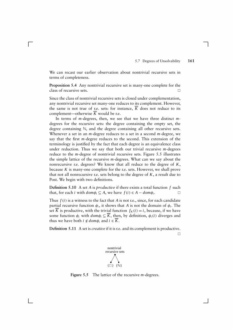
5.7 Degrees of Unsolvability 161
We can recast our earlier observation about nontrivial recursive sets interms of completeness.
Proposition 5.4 Any nontrivial recursive set is many-one complete for theclass of recursive sets. h
Since the class of nontrivial recursive sets is closed under complementation,any nontrivial recursive set many-one reduces to its complement. However,the same is not true of r.e. sets: for instance, K does not reduce to itscomplement—otherwise K would be r.e.
In terms of m-degrees, then, we see that we have three distinct m-degrees for the recursive sets: the degree containing the empty set, thedegree containing N, and the degree containing all other recursive sets.Whenever a set in an m-degree reduces to a set in a second m-degree, wesay that the first m-degree reduces to the second. This extension of theterminology is justified by the fact that each degree is an equivalence classunder reduction. Thus we say that both our trivial recursive m-degreesreduce to the m-degree of nontrivial recursive sets. Figure 5.5 illustratesthe simple lattice of the recursive m-degrees. What can we say about thenonrecursive r.e. degrees? We know that all reduce to the degree of K ,because K is many-one complete for the r.e. sets. However, we shall provethat not all nonrecursive r.e. sets belong to the degree of K , a result due toPost. We begin with two definitions.
Definition 5.10 A set A is productive if there exists a total function f suchthat, for each i with domφi ⊆ A, we have f (i) ∈ A − domφi . h
Thus f (i) is a witness to the fact that A is not r.e., since, for each candidatepartial recursive function φi , it shows that A is not the domain of φi . Theset K is productive, with the trivial function fK (i)= i , because, if we havesome function φi with domφi ⊆ K , then, by definition, φi (i) diverges andthus we have both i /∈ domφi and i ∈ K .
Definition 5.11 A set is creative if it is r.e. and its complement is productive.h
nontrivial recursive sets
{∅} {N}
Figure 5.5 The lattice of the recursive m-degrees.

162 Computability Theory
For instance, K is creative. Notice that an r.e. set is recursive if and only ifits complement is r.e.; but if the complement is productive, then we havewitnesses against its being r.e. and thus witnesses against the original set’sbeing recursive.
Theorem 5.9 An r.e. set is many-one complete for the class of r.e. sets ifand only if it is creative. h
Proof. We begin with the “only if” part: assume the C is many-onecomplete for r.e. sets. We need to show that C is creative or, equivalently,that C is productive. Since C is complete, K reduces to C through somefunction f = φm . Now define the new function
ψ(x, y, z)= φuniv(x, φuniv(y, z))= φx (φy(z))
By the s-m-n theorem, there exists a recursive function g(x, y) withφg(x,y)(z)= ψ(z). We claim that the recursive function h(x)= f (g(x, m))is a productive function for C . Assume then that we have some function φi
with domφi ⊆ C and consider h(i)= f (g(i,m)); we want to show that h(i)belongs to C − domφi . We have
f (g(i,m)) ∈ C ⇔ g(i, m) ∈ K
⇔ φg(i,m)(g(i, m)) ↑
⇔ φi (φm(g(i,m))) ↑
⇔ φi ( f (g(i,m))) ↑
It thus remains only to verify that f (g(i,m)) does not belong to C. But, iff (g(i,m))were to belong to C, then (from the above) φi ( f (g(i,m)))wouldconverge and f (g(i, m)) would belong to domφi , so that we would havedomφi 6⊆ C, a contradiction.
Now for the “if” part: let C be a creative r.e. set with productivefunction f , and let B be an r.e. set with domain function φB . We needto show that B many-one reduces to C. Define the new function ψ(x, y, z)to be totally undefined if y is not in B (by invoking Zero(φB(y))) andto be otherwise defined only for z = f (x). By the s-m-n theorem, thereexists a recursive function g(x, y) with ψ(x, y, z)= φg(x,y)(z) and, by therecursion theorem, there exists a fixed point xy with φxy(z)= φg(xy ,y)(z). Bythe extended recursion theorem, this fixed point can be computed for eachy by some recursive function e(y)= xy. Thus we have
domφe(y) = domφg(e(y),y) =
{
{ f (e(y))} y ∈ B
∅ otherwise
5.7 Degrees of Unsolvability 163
But C is productive, so that domφe(y) ⊆ C implies f (e(y))∈ C − domφe(y).Hence, if y belongs to B, then the domain of φe(y) is { f (e(y))}, in whichcase f (e(y)) cannot be a member of C − domφe(y), so that domφe(y) is not asubset of C and f (e(y))must be a member of C. Conversely, if y does notbelong to B, then domφe(y) is empty and thus a subset of C, so that f (e(y))belongs to C. Hence we have reduced B to C through f · e. Q.E.D.
Therefore, in order to show that there exist r.e. sets of different m-degrees,we need only show that there exists noncreative r.e. sets.
Definition 5.12 A simple set is an r.e. set such that its complement is infinitebut does not contain any infinite r.e. subset. h
By Exercise 5.28, a simple set cannot be creative.
Theorem 5.10 There exists a simple set. h
Proof. We want a set S which, for each x such that φx has infinitedomain, contains an element of that domain, thereby preventing it frombeing a subset of S. We also want to ensure that S is infinite by “leaving out”of S enough elements. Define the partial recursive function ψ as follows:
ψ(x)=51(µy[51(y) > 2x and step(x, 51(y), 52(y)) 6= 0])
Now let S be the range of ψ ; we claim that S is simple. It is clearly r.e.,since it is the range of a partial recursive function. When ψ(x) converges,it is larger than 2x by definition, so that S contains at most half of themembers of any initial interval of N; thus S is infinite. Now let domφx beany infinite r.e. set; because the domain is infinite, there is a smallest y suchthat we have 51(y) > 2x , 51(y) ∈ domφx , and step(x, 51(y), 52(y)) 6= 0.Then ψ(x) is 51(y) for that value of y, so that 51(y) belongs to S and thedomain of φx is not a subset of S. Q.E.D.
Since a simple set is not creative, it cannot be many-one complete for ther.e. sets. Since K is many-one complete for the r.e. sets, it cannot be many-one reduced to a simple set and thus cannot belong to the same m-degree.Hence there are at least two different m-degrees among the nonrecursiver.e. sets. In fact, there are infinitely many m-degrees between the degree ofnontrivial recursive sets and the degree of K , with infinitely many pairs ofincomparable degrees—but the proofs of such results lie beyond the scopeof this text. We content ourselves with observing that our Infinite Hotelstory provides us with an easy proof of the following result.
Theorem 5.11 Any two m-degrees have a least upper-bound. h
164 Computability Theory
In other words, given two m-degrees ! and @, there exists an m-degree #
such that (i) ! and @ both reduce to # and (ii) if ! and @ both reduce toany other m-degree $, then # reduces to $.
Proof. Let ! and @ be our two m-degrees, and pick A ∈ ! and B ∈ @.Define the set C by C = {2x | x ∈ A} ∪ {2x + 1 | x ∈ B}—the trick used in theInfinite Hotel. Clearly both A and B many-one reduce to C. Thus both !
and @ reduce to #, the m-degree containing, and defined by, C. Let $ besome m-degree to which both ! and @ reduce. Pick some set D ∈ $, andlet f be the reduction from A to D and g be the reduction from B to D.We reduce C to D by the simple mapping
h(x)=
{
f ( x2 ) x is even
g( (x−1)2 ) x is odd
Hence # reduces to $. Q.E.D.
The m-degrees of unsolvability of the r.e. sets form an upper semilattice.
5.8 Exercises
Exercise 5.11 Prove that the following functions are primitive recursive bygiving a formal construction.
1. The function exp(n, m) is the exponent of the the mth prime in theprime power decomposition of n, where we consider the 0th primeto be 2. (For instance, we have exp(1960, 2)= 1 because 1960 has asingle factor of 5.)
2. The function max y ø x[g(y, z1, . . ., zn)], where g is primitive recur-sive, returns the largest value in {g(0, . . . ), g(1, . . . ), . . . , g(x, . . . )}.
3. The Fibonacci function F(n) is defined by F(0) = F(1) = 1 andF(n)= F(n − 1)+ F(n − 2). (Hint: use the course-of-values recursiondefined in Equation 5.1.)
Exercise 5.12 Verify that iteration is primitive recursive. A function f isconstructed from a function g by iteration if we have f (x, y)= gx(y), wherewe assume g0(y)= y.
Exercise 5.13 Verify that the function f defined as follows:
{
f (0, x)= g(x)
f (i + 1, x)= f (i, h(x))
is primitive recursive whenever g and h are.

5.8 Exercises 165
Exercise 5.14 Write a program (in the language of your choice) to computethe values of Ackermann’s function and tabulate the first few values—butbe careful not to launch into a computation that will not terminate in yourlifetime! Then write a program that could theoretically compute the valuesof a function at a much higher level in the Grzegorczyk hierarchy.
Exercise 5.15 Prove that the following three sets are not recursive byexplicit reduction from the set K —do not use Rice’s theorem.
1. {x | φx is a constant function}
2. {x | φx is not the totally undefined function}
3. {x | there is y with φx (y) ↓ and such that φy is total}
Exercise 5.16 For each of the following sets and its complement, classifythem as recursive, nonrecursive but r.e., or non-r.e. You may use Rice’stheorem to prove that a set is not recursive. To prove that a set is r.e., showthat it is the range or domain of a partial recursive function. For the rest,use closure results or reductions.
1. S(y)= {x | y is in the range of φx}.
2. {x | φx is injective}.
3. The set of all primitive recursive programs.
4. The set of all (mathematical) primitive recursive functions.
5. The set of all partial recursive functions that grow at least as fast asn2.
6. The set of all r.e. sets that contain at least three elements.
7. The set of all partial recursive functions with finite domain.
8. The three sets of Exercise 5.15.
Exercise 5.17 Prove formally that the Busy Beaver problem is undecidable.The busy beaver problem can be formalized as follows: compute, for eachfixed n, the largest value that can be printed by a program of length n (thathalts after printing that value). This question is intuitively the converse ofTheorem 5.5.
Exercise 5.18 Let S be an r.e. set; prove that the sets D =⋃
x∈S domφx andR =
⋃
x∈S ranφx are both r.e.
Exercise 5.19 Let Kt be the set {x | ∃y ø t, step(x, x, y) > 0}; that is, Kt isthe set of functions that converge on the diagonal in at most t steps.
1. Prove that, for each fixed t , Kt is recursive, and verify the equality⋃
t∈NKt = K .
2. Conclude that, if S is an r.e. set, the set⋂
x∈S domφx need not be r.e.

166 Computability Theory
Exercise 5.20 Prove that every infinite r.e. set has an injective enumeratingfunction (that is, one that does not repeat any element).
Exercise 5.21 Prove that an infinite r.e. set is recursive if and only if it hasan injective, monotonically increasing enumerating function.
Exercise 5.22 Let S = {{i, j} | φi and φ j compute the same function}. Is Srecursive, nonrecursive but r.e., or non-r.e.?
Exercise 5.23 Define the following two disjoint sets: A = {x | φx (x)= 0} andB = {x | φx(x)= 1}. Prove that both sets are nonrecursive but r.e. (the sameproof naturally works for both) and that they are recursively inseparable,i.e., that there is no recursive set C with A ⊆ C and B ⊆ C . Such a setwould recursively separate A and B in the sense that it would draw arecursive boundary dividing the elements of A from those of B. (Hint: usethe characteristic function of the putative C to derive a contradiction.)
Exercise 5.24 This exercise explores ways of defining partial functions thatmap finite subsets of N to N. Define the primitive recursive function
f (i, x)=5Succ(51(i))Succ(x) (52(i))
1. Define the sequence of partial recursive functions {ψi } by
ψi (x)=
{
f (i, x) x < Succ(51(i))
undefined otherwise
Verify that this sequence includes every function that maps a nonemptyfinite initial subset of N (i.e., some set {0, 1, . . . , k}) to N.
2. Define the sequence of partial recursive functions {πi } by
πi (x)=
{
dec( f (i, x)) x < Succ(51(i)) and f (i, x) > 0
undefined otherwise
Verify that this sequence includes every function that maps a finitesubset of N to N.
Exercise 5.25∗ This exercise develops the Rice-Shapiro theorem, whichcharacterizes r.e. sets in much the same way as Rice’s theorem charac-terizes recursive sets. The key to extending Rice’s theorem resides in finiteinput/output behaviors, each of which defines a recursive set. In essence, aclass of partial recursive functions is r.e. if and only if each partial recursivefunction in the class is the extension of some finite input/output behavior

5.9 Bibliography 167
in an r.e. set of such behaviors. Exercise 5.24 showed that the sequence {πi }
captures all possible finite input/output behaviors; our formulation of theRice-Shapiro theorem uses this sequence.
Let # be any class of (mathematical) partial recursive functions. Thenthe set {x | φx ∈ #} is r.e. if and only if there exists an r.e. set I with
φx ∈ # ⇔ ∃i ∈ I, πi ⊆ φx
(where πi ⊆ φx indicates that φx behaves exactly like πi on all arguments onwhich πi is defined—and may behave in any way whatsoever on all otherarguments).
Exercise 5.26 Use the recursion theorem to decide whether there are indiceswith the following properties:
1. The domain of φn is {n2}.2. The domain of φn is N − {n}.3. The domain of φn is K and also contains n.
Exercise 5.27 Prove that the set S(c)= {x | c /∈ domφx}, where c is anarbitrary constant, is productive.
Exercise 5.28 Prove that every productive set has an infinite r.e. subset.
Exercise 5.29 Let S be a set; the cylindrification of S is the set S × N. Provethe following results about cylinders:
1. A set and its cylindrification belong to the same m-degree.2. If a set is simple, its cylindrification is not creative.
Exercise 5.30∗ Instead of using many-one reductions, we could have usedone-one reductions, that is, reductions effected by an injective function.One-one reductions define one-degrees rather than m-degrees. Revisit allof our results concerning m-degrees and rephrase them for one-degrees.Recursive sets now get partitioned into finite sets of each size, infinite setswith finite complements, and infinite sets with infinite complements. Notealso that our basic theorem about creative sets remains unchanged: an r.e.set is one-complete for the r.e. sets exactly when it is complete. Do a set andits cylindrification (see previous exercise) belong to the same one-degree?
5.9 Bibliography
Primitive recursive functions were defined in 1888 by the German mathe-matician Julius Wilhelm Richard Dedekind (1831–1916) in his attempt to
168 Computability Theory
provide a constructive definition of the real numbers. Working along thesame lines, Ackermann [1928] defined the function that bears his name.Godel [1931] and Kleene [1936] used primitive recursive functions again,giving them a modern formalism. The course-of-values mechanism (Equa-tion 5.1) was shown to be closed within the primitive recursive functionsby Peter [1967], who used prime power encoding rather than pairing inher proof; she also showed (as did Grzegorczyk [1953]) that the boundedquantifiers and the bounded search scheme share the same property.
Almost all of the results in this chapter were proved by Kleene [1952].The first text on computability to pull together all of the threads developedin the first half of the twentieth century was that of Davis [1958]. Rogers[1967] wrote the classic, comprehensive text on the topic, now reissued byMIT Press in paperback format. A more modern treatment with much thesame coverage is offered by Tourlakis [1984]. An encyclopedic treatmentcan be found in the two-volume work of Odifreddi [1989], while the textof Pippenger [1997] offers an advanced treatment. Readers looking fora strong introductory text should consult Cutland [1980], whose shortpaperback covers the same material as our chapter, but in more detail. Inmuch of our treatment, we followed the concise approach of Machtey andYoung [1978], whose perspective on computability, like ours, was stronglyinfluenced by modern results in complexity.
The text of Epstein and Carnielli [1989] relates computability theory tothe foundations of mathematics and, through excerpts from the original ar-ticles of Hilbert, Godel, Kleene, Post, Turing, and others, mixed with criticaldiscussions, offers much insight into the development of the field of com-putability. Davis [1965] edited an entire volume of selected reprints fromthe pioneers of the 1930s—from Hilbert to Godel, Church, Kleene, Turing,Post, and others. These articles are as relevant today as they were then andexemplify a clarity of thought and writing that has become too rare.
Berry’s paradox has been used by Chaitin [1990a,1990b] in build-ing his theory of algorithmic information theory, which grew from anoriginal solution to the question of “what is a truly random string”—to which he and the Russian mathematician Kolmogorov answered “anystring which is its own shortest description.” Chaitin maintains, at URLhttp://www.cs.auckland.ac.nz/CDMTCS/chaitin/, a Web sitewith much of his work on-line, along with tools useful in exploring someof the consequences of his results.