compression domain volume rendering for distributed
TRANSCRIPT

EUROGRAPHICS ‘98 Tutorial
© 1998 Institute of Scientific Computing, Department of Computer Science, Swiss Fed-eral Institute of Technology (ETH) Zurich, Switzerland.
Compression DomainVolume Rendering for Distributed Environments
L. Lippert, M. H. Gross, C. Kurmann
Department of Computer Science, ETH Zürich
Email: {lippert, grossm, kurmann}@inf.ethz.chWWW: http://www.inf.ethz.ch/department/WR/cg
Abstract
This paper describes a method for volume data compression and rendering which bases on wavelet splats. Theunderlying concept is especially designed for distributed and networked applications, where we assume aremote server to maintain large scale volume data sets, being inspected, browsed through and rendered inter-actively by a local client. Therefore, we encode the server‘s volume data using a newly designed wavelet basedvolume compression method. A local client can render the volumes immediately from the compression domainby using wavelet footprints, a method proposed earlier. In addition, our setup features full progression, wherethe rendered image is refined progressively as data comes in. Furthermore, framerate constraints are consid-ered by controlling the quality of the image both locally and globally depending on the current network band-width or computational capabilities of the client. As a very important aspect of our setup, the client does notneed to provide storage for the volume data and can be implemented in terms of a network application. Theunderlying framework enables to exploit all advantageous properties of the wavelet transform and forms abasis for both sophisticated lossy compression and rendering. Although coming along with simple illuminationand constant exponential decay, the rendering method is especially suited for fast interactive inspection oflarge data sets and can be supported easily by graphics hardware.
Keywords: volume rendering, multiresolution, progressive compression, splatting, wavelets, networks, dis-tributed applications
1. Introduction
Volume rendering, in general, has been a very importantsubfield of research in computer graphics. Since its inven-tion [12], [16], countless algorithms have been proposed,[13], [14], most of which have been designed for providinghigh quality images at low computational efforts. In thiscontext, recent advancements in graphics hardware help toexploit individual capabilities of graphics workstations [2].If real time performance constrains the method and imagequality can be relaxed, so-called splatting methods [15], [4]have proved to provide good results. Here, footprints of avolume primitive are computed in terms of a small pixmaptexture and are superimposed in the framebuffer to carry outthe final image. Introducing hierarchical basis functions,such as wavelets [17], rendering is carried out progressivelyby accumulating scaled and translated versions of self-simi-lar textures.
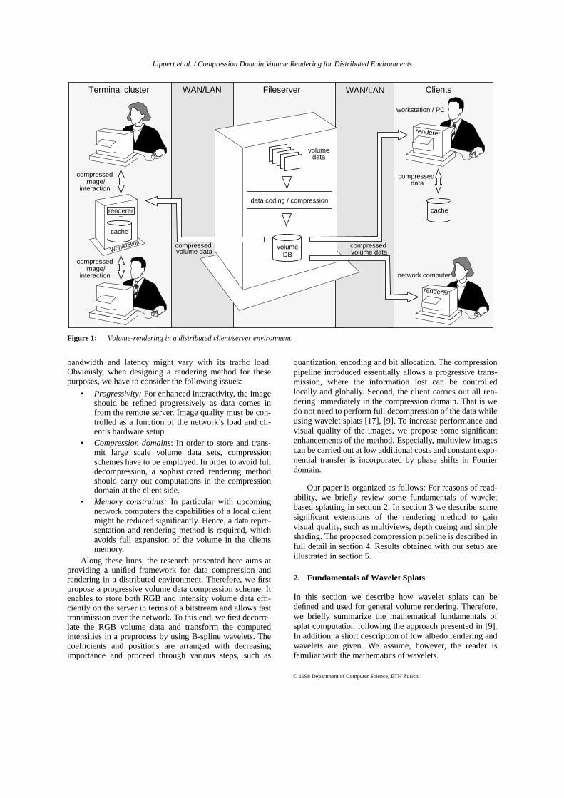
Unfortunately, most rendering methods introduced sofar relate to local computation environments. The problemsarising with distributed environments and associated com-pression domain rendering has hardly been addressed in theliterature [24], [10]. However, in times of distributed, worldwide information systems and exponentially increasing vol-ume data sets, requirements for rendering such data havechanged. In many application scenarios, such as in medicalimaging and information systems, situations arise, such asdepicted in figure 1.
Often, volume data sets are stored and maintained by adata base server, which can be accessed by one or morelocal clients via a network. One of the fundamental tasks ofvolume rendering is to inspect interactively and to browsethrough the volume data base, where rendering quality canbe relaxed for the sake of real time performance. Moreover,being a low end workstation, the computational power andstorage capacity of the client are limited and the network‘s
Lippert et al. / Compression Domain Volume Rendering for Distributed Environments
© 1998 Department of Computer Science, ETH Zurich.
bandwidth and latency might vary with its traffic load.Obviously, when designing a rendering method for thesepurposes, we have to consider the following issues:
• Progressivity:For enhanced interactivity, the imageshould be refined progressively as data comes infrom the remote server. Image quality must be con-trolled as a function of the network’s load and cli-ent’s hardware setup.
• Compression domains: In order to store and trans-mit large scale volume data sets, compressionschemes have to be employed. In order to avoid fulldecompression, a sophisticated rendering methodshould carry out computations in the compressiondomain at the client side.
• Memory constraints:In particular with upcomingnetwork computers the capabilities of a local clientmight be reduced significantly. Hence, a data repre-sentation and rendering method is required, whichavoids full expansion of the volume in the clientsmemory.
Along these lines, the research presented here aims atproviding a unified framework for data compression andrendering in a distributed environment. Therefore, we firstpropose a progressive volume data compression scheme. Itenables to store both RGB and intensity volume data effi-ciently on the server in terms of a bitstream and allows fasttransmission over the network. To this end, we first decorre-late the RGB volume data and transform the computedintensities in a preprocess by using B-spline wavelets. Thecoefficients and positions are arranged with decreasingimportance and proceed through various steps, such as
quantization, encoding and bit allocation. The compressionpipeline introduced essentially allows a progressive trans-mission, where the information lost can be controlledlocally and globally. Second, the client carries out all ren-dering immediately in the compression domain. That is wedo not need to perform full decompression of the data whileusing wavelet splats [17], [9]. To increase performance andvisual quality of the images, we propose some significantenhancements of the method. Especially, multiview imagescan be carried out at low additional costs and constant expo-nential transfer is incorporated by phase shifts in Fourierdomain.
Our paper is organized as follows: For reasons of read-ability, we briefly review some fundamentals of waveletbased splatting in section 2. In section 3 we describe somesignificant extensions of the rendering method to gainvisual quality, such as multiviews, depth cueing and simpleshading. The proposed compression pipeline is described infull detail in section 4. Results obtained with our setup areillustrated in section 5.
2. Fundamentals of Wavelet Splats
In this section we describe how wavelet splats can bedefined and used for general volume rendering. Therefore,we briefly summarize the mathematical fundamentals ofsplat computation following the approach presented in [9].In addition, a short description of low albedo rendering andwavelets are given. We assume, however, the reader isfamiliar with the mathematics of wavelets.
Figure 1: Volume-rendering in a distributed client/server environment.
volumeDB
data coding / compression
cache
cache
volumedata
Workstation compressed
compressed
compressedvolume data
compressed
interaction
Fileserver ClientsTerminal cluster WAN/LANWAN/LAN
volume data
network computer
workstation / PC
renderer+
renderer
renderer
data image/
compressed
interaction image/

Lippert et al. / Compression Domain Volume Rendering for Distributed Environments
© 1998 Department of Computer Science, ETH Zurich.
2.1. Low Albedo Volume Rendering
Volume rendering can be regarded as a composition of par-ticles that, in addition to their own emission, receive lightfrom surrounding lightsources and reflect these intensitiestowards the observer.
In classic volume rendering, the amount of lightreceived at pointx from directions up to a ray
lengthtL is computed as:
(1)
where q denotes the volume source term andα theopacity function. For an isotropic medium with constantopacity equation (1) reduces to
(2)
In particular note that for we end up in a X-ray-like image.
Especially in those cases, splatting has proved itsusability for fast volume rendering [15]. In contrast to ray-casting, it allows to reduce the computational complexityfor interpolation and integration to a minimum, since thepreprojected footprints of high-order interpolation func-tions can be stored as lookup tables. The projections them-selves can be computed with an accurate quadraturetechnique. Besides hierarchical splats [15], wavelet splat-ting [17] is a sophisticated extension.
2.2. B-spline Wavelets
Since we aim at a unified data representation for both vol-ume data compression and rendering, we use Chui andWang [3] B-spline wavelet bases of orderj. They havemany usefull properties, such as smoothness and vanishingmoments. In addition, analytic expressions for scaling- andwavelet functions and their duals in the frequency- and spa-tial-domain are given. The mother-scaling function of order1 is defined as:
(3)
Compactly supported scaling functions of orderj can begenerated recursively in terms of cardinal B-splines:
(4)
In the frequency-domain the corresponding functionscollapse intosinc-polynomials of type:
(5)
In the upper termf denotes the frequency andi the com-plex operator. Note, that the upper equation is fundamentalfor splat computation in Fourier domain. The semiorthogo-nality of the function system forj > 1 requires duals. For thecase of B-spline wavelets all primary and dual functionshave linear phase. Furthermore, only rational coefficientshave to be used for the fast wavelet transform.
To fully characterize the wavelet transform, we need todetermine the wavelet functions. For the correspondingwavelets we obtain:
(6)
Note, that their support can be computed straightfor-wardly as [0,2j-1]. Wavelets in three dimensions areobtained easily by non-standard tensor-product extensions[5].
Here volume decomposition is carried out with theduals, whereas reconstruction is performed using the pri-mary functions (4), (6). Note furthermore, that implementa-tions of linear time algorithms [20] can be morechallenging, since additional basis transforms might berequired.
2.3. Construction of Wavelet Splats
In wavelet splatting, the renderer computes the projectionsuch as defined in (2). Taking into account the waveletdecomposition levelm up toM and moving the summationoutside the integral, the formulation collapses to:
(7)
where denote the wavelet coefficients of decom-
position levelm at the spatial positionp, q, r and wavelet-type typeand the coefficient of the scaling function
of level M. The computation of the line integrals for a par-ticular view can be accomplished by Fourier projection slic-ing (FPS). It allows to compute accurate projections of anybasis function. This theorem states that the 2D Fouriertransform of a projection of a functionf(x,y,z) onto a givenplane P equals a plane that slices the Fourier transform
parallel toP and intersects the origin.
Since many wavelet types such as B-splines come alongwith closed form representations in the frequency domain,it is straightforward to apply this theorem to get therequired splats. Figure 2 depicts the setting, where aninverse FFT processes the slices to obtain the wavelet splat.
I t L x s, ,( )
I t L x s, ,( ) q x t s⋅+( )e
α x su+( ) ud
0
t
∫–
td
0
tL
∫=
α
I t L x s, ,( ) q x t s⋅+( )e α– ttd
0
tL
∫=
α 0≡
φ 1[ ] x( ) 1 0 x 1<≤0 otherwise
=
φ j[ ] x( )x
j 1–-----------φ j 1–[ ] x( )
j x–j 1–-----------φ j 1–[ ] x 1–( )+=
Φ j[ ] f( ) 1 ei2πf–
–i2πf
-----------------------
j
=
ψ j[ ] x( ) qj k, φ j[ ] 2x k–( )k 0=
3 j 2–
∑=
with qj k,1–( )k
2 j 1–------------- j
l φ 2 j[ ] k 1 l–+( )
l 0=
j
∑=
I ∞ x s, ,( ) dmpqrtype ψmpqr
3 type, x st+( ) td
∞–
∞
∫type 1=
p q r Z∈, ,
7
∑m 1=
M
∑=
cMpqr φMpqr3 x st+( ) td
∞–
∞
∫p q r Z∈, ,
∑+
dmpqrtype
cMpqr
F ω1 ω2 ω3, ,( )

Lippert et al. / Compression Domain Volume Rendering for Distributed Environments
© 1998 Department of Computer Science, ETH Zurich.
The intersection plane spanned byu, v defines the 2DFourier transform of the texture splats
, whereas the
normal vectorn of the plane equals the direction of the pro-jection. The definition of the viewing parameters is figuredout in spherical coordinates (α,β).
Once the renderer builds the viewpoint dependent inte-gral tables, the screen position of the table is calculated,mapped, weighted by the wavelet coefficient and accumu-lated into the framebuffer. Since the basis functions of dif-ferent iteration levelsm differ by dilation, only eightdifferent splats of depthM have to be calculated. All otherfootprints are derived by subsampling in the spirit of amipmap. Correct sampling and optimized data-structures ofthe calculated splats are discussed in [9].
3. Visual Enhancements
We are now in a position to discuss two significant render-ing features which help to improve the visual quality of thegenerated images. In particular, we introduce a method forthe computation of multiviews, being important in manyapplications, such as medical imaging. Exploiting the sym-metry of 3D tensor-product wavelets allows the additionalcosts to be kept sufficiently low. Furthermore, we addressthe problem of exponential transfer functions in Fourierspace. Phase shifts of the wavelet’s FT enable exponentialtransfer to be incorporated and can be used to simulateshading operations on the fly.
3.1. Multiviews
The rendered images, obtained by our splatting approach,lack occlusion. Since this important visual cue is missingfor the calculated X-ray images, depth information is notpresented to the user. One way to overcome this drawbackis the introduction of a multiview arrangement. Here, thevolume is rendered simultaneously from different directionsand presented to the user in a single window. Exploiting thecoherence of different viewing angles given by the symme-try of tensor-product constructions, the basic single-viewsplatting approach can be extended to a multiview rendererwithout computational overhead for splat computation. Werecall that the tensor-product functions are constructed frompermutations of the 1D basis functions and along thex, y andz directions.
Figure 3 exemplifies the idea. The footprint of the basis
function (3D Haar scaling function of level 0,
aligned to the origin) from the first viewing-direction equalsthe footprint from the second and third direction, e.g. thecalculated footprints can be reused for rendering differentviews. Thus, we propose to generate a lookup table for thebasis functions types 1 to 7 to ensure correct footprint cal-culation. A corresponding lookup table is given in Table 1and illustrated in figure 4 for Haar functions respectively.
In order to combine the three footprints for the eightdifferent basis functions, eight textures are calculated forview 1 by the FPS-theorem. The footprint for the basisfunction is equal for view 1 and 2, whereas the splat
of the view 3 is given by the footprint of the function(texture 4) of view 1. The corresponding permutations are
I u v,( ) F ω1 u v,( ) ω2 u v,( ) ω3 u v,( ), ,( )=
Figure 2: Illustration of the Fourier projection slicing theorem in 3D for an idealized Shannon wavelet.
ω1
ω2 slicing plane
Φ ω1 ω2 ω3, ,
u
v
φ x µ ν t, ,( ) y µ ν t, ,( ) z µ ν t, ,( ), ,( )
∞–
∞
∫ dt
ν
µ
slic
ing
iFF
T
frequency domain spatial domain
Φ u v,( )
frequency domain
α
β
u
v
n
ω3
φ ψ
Figure 3: Illustration of the multiview concept.
Table 1: Permutations and negations for multi view arrange-ments
PERMUTATIONS NEGATIONS
VIEW 1 [ 0 1 2 3 4 5 6 7 ] [ 1 1 1 1 1 1 1 1 ]
VIEW 2 [ 0 1 4 5 2 3 6 7 ] [ 1 1 -1 -1 1 1 -1 -1]
VIEW 3 [ 0 4 2 6 1 5 3 7 ] [ 1 1 1 1 -1 -1 -1 -1 ]
y
z
x
view 2
view 1
view
3view 1view 2
view 3φ00003 1[ ]
φ00003 1[ ]
φφψψφφ

Lippert et al. / Compression Domain Volume Rendering for Distributed Environments
© 1998 Department of Computer Science, ETH Zurich.
given for all basis functions and for three views in Table 1.In some cases it is also necessary to multiply the intensitywith -1. The same permutation tables can also be used forhigher order wavelets.
Note that these permutations are equal for each viewingdirection. Note furthermore that the angles between theindividual viewing planes are not constant. Moreover, theydepend on the initial selection of the camera parameters. Alittle algebra reveals that the three projection-planesPi,spanned by the vectors (ui,vi) are given by
View 1: with
View 2: with
View 3: with
The triple view rendering is illustrated in figure 5,where a classified data set is displayed from three direc-tions. The image was grabbed directly from the screen as itis displayed to the user. Skin is colored white, brain tissuered and a tumor is colored in blue.
3.2. Depth Cueing
Up to now, only linear depth cueing has been considered inthe frequency domain [22]. In order to compute constantexponential decay as in (2) we propose a depth cueingapproach implemented as a two step solution. In the firststep the cued footprints have to be calculated by the FPS-theorem and an additional phase-shift. Second, the textureshave to be weighted according to the distance between theprojection plane and the basis functions.
Footprint Computation In order to set up the Fourierrelations for exponentially weighted functions, let’s firstconsider the relations in the spatial domain. Letdenote the function that is depth cued alongt and letk bethe constant exponential extinction coefficient. We obtain
the new function as:
(8)
In the frequency domain the Fourier transform ofcan be written as:
(9)
Obviously, the Fourier transform of the exponentially
depth-cued function is computed by shiftingwith the imaginary frequencyf0. This can be interpreted as
Figure 4: Different wavelet types figured out by non-standardtensor-product extensions for the Haar case.
u1 v1,( )
u1
αsin–
αcos
0
ux
uy
uz
= = v1
αcos– βsin
αsin– βsin
βcos
vx
vy
vz
= =
u2 v2,( )
u2
αcos–
αsin–
0
u– y
ux
uz
= = v2
αsin– βsin
αcos βsin
βcos
v– y
vx
vz
= =
u3 v3,( )
u3
0
αcos
αsin
uz
uy
u– x
= = v3
βcos–
αsin– βsin
αcos βsin
v– z
vy
v– x
= =
++
++
+
+
++
++
+
+ --
--
--
+
+++
--
--
+++
-- -
--
+++
+
++
+
++
++
++
+
+-
--
---
++
---
---
+++
+
+
+ -
--
-
--
-+
+++
--
++
View 1View 2
View 3
Tex5ψφψ Tex6ψψφ Tex7ψψψ
Tex3φψψTex2φψφTex1φφψTex0φφφ
Tex4ψφφ
-
--
---
+
--
+++
Figure 5: Triple views seen from different viewing angles as ap-plied to classified MR-data set (volume size: 256 x 128 x 256, max.decomposition level M = 2) a)α = β = 0.0 b)α = 0.66,β = 0.91.
a) b)
h t( )
h̃ t( )
h̃ t( ) h t( )ekt=
h t( )ei2π f 0t–
where= f 0k2πi–
----------- ki2π------= =
h̃ t( )
H̃ f( ) h̃ t( )ei2πfttd
∞–
∞
∫=
h t( )ei2π f f 0–( )t
td
∞–
∞
∫=
H f f 0–( )=
h̃ t( ) H f( )

Lippert et al. / Compression Domain Volume Rendering for Distributed Environments
© 1998 Department of Computer Science, ETH Zurich.
a “frequency phase shift”. For the B-spline scaling func-tions and wavelets of orderj in the frequency domain wehave
(10)
where
(11)
In 3D the direction of the shift operation in the spec-trum can be chosen without any restriction and indepen-dently from the viewing direction. It corresponds to thedepth-cueing direction in the spatial domain. We define thecueing vectorL for any pair of viewing angles (αl , βl) as
(12)
to determine the cueing direction and extinction coeffi-cient. Figure 6 shows the calculated splats resulting fromthis method.
Distance Weighting For correct depth cueing of the vol-ume, the computed footprints have to be weighted accord-ing to their distance from a reference plane which can beregarded as a planar light source, perpendicular to thedepth-cueing vectorL that points towards the volume mid-point VM. Let L init represent the intersection point of thevolume’s bounding sphere and its tangent plane, the weight-ing factorωd for each basis function centered atBM= P +L init can be computed as:
(13)
During the accumulation process this factor is multi-plied with the wavelet coefficient and the accumulation stepproceeds straightforwardly. The geometric relationships aredepicted in figure 7.
As a result we come up with smooth and correctlydepth-cued volumes, such as shown in figure 6.
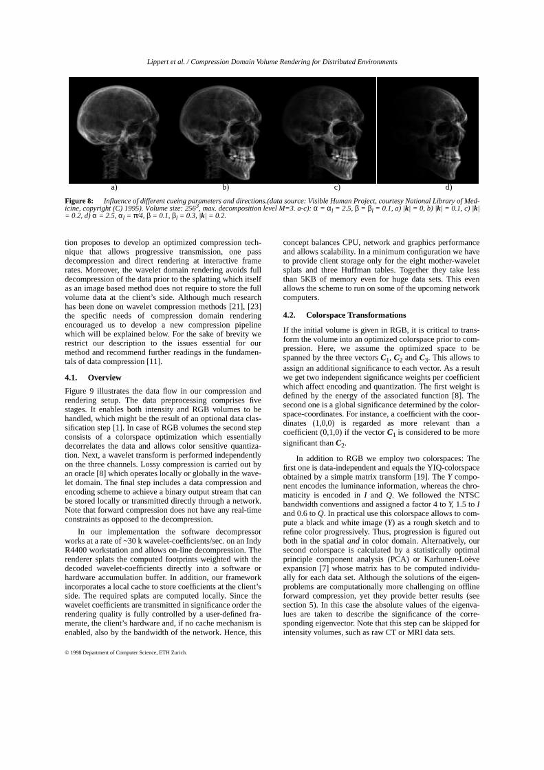
To illustrate the performance of our method, we appliedthe approach to the visible human CT-data set [18]. Theinfluence of different factors |k| and different cueing direc-tions are displayed in figure 8 Note that exponential depthcueing increases the rendering performance, since less tex-tures have to be accumulated. Moreover, interactive manip-ulation of the cueing direction allows us to simulate simpleshading operations in the wavelet domain and enhances thevisual quality significantly.
4. Progressive Compression and Transmission
As motivated earlier, our approach is targeted at networkedapplications where, for instance, a local client with lowcomputational power browses through a remote database.Thus, in order to transmit our volume data efficiently wehave to find appropriate compression strategies. It is clearthat the underlying framework of the wavelet decomposi-
Φ̃ j[ ] f( ) 1 ei2π f f 0–( )–
–i2π f f 0–( )
-----------------------------------
j
=
Ψ̃ j[ ] f( ) R j[ ] ei π f f 0–( )–
Φ̃ j[ ] f
2---
=
R j[ ] ei π f f 0–( )–
1
2--- qj n, e
i π f f 0–( )–
n
⋅n ∞–=
∞
∑=
L αl βl,( ) k
αlcos– βlcos
αsin l βlcos
βlsin
kx
ky
kz
= =
ωd e dist–= where distL P⋅
L------------=
Figure 6: Exponentially depth-cued scaling function (j=1) a)|k|=0.0. b) |k|=0.6. Distance weighted footprints: c) depth cuedsplats without distance weighting, d) corrected splats using dis-tance weighting.
Figure 7: Geometric relationships for distance-weighting of ba-sis functions.
t
L
φ
t
L
φ
c) d)
t t
LL
φ φ
a) b)
x
z
y
Ldist
bounding sphereof volume data set
LinitBM
VM
planar light source
P
(tangent plane ofbounding sphere)

Lippert et al. / Compression Domain Volume Rendering for Distributed Environments
© 1998 Department of Computer Science, ETH Zurich.
tion proposes to develop an optimized compression tech-nique that allows progressive transmission, one passdecompression and direct rendering at interactive framerates. Moreover, the wavelet domain rendering avoids fulldecompression of the data prior to the splatting which itselfas an image based method does not require to store the fullvolume data at the client’s side. Although much researchhas been done on wavelet compression methods [21], [23]the specific needs of compression domain renderingencouraged us to develop a new compression pipelinewhich will be explained below. For the sake of brevity werestrict our description to the issues essential for ourmethod and recommend further readings in the fundamen-tals of data compression [11].
4.1. Overview
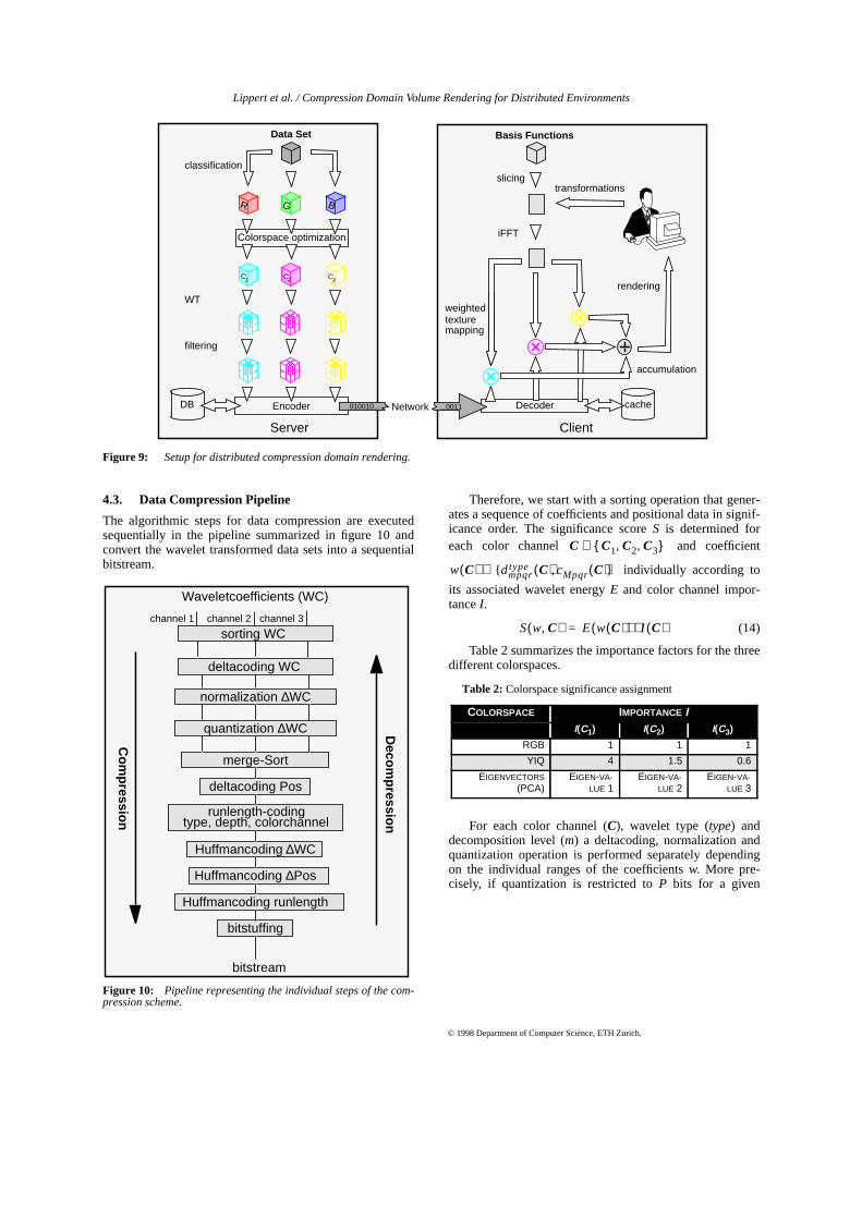
Figure 9 illustrates the data flow in our compression andrendering setup. The data preprocessing comprises fivestages. It enables both intensity and RGB volumes to behandled, which might be the result of an optional data clas-sification step [1]. In case of RGB volumes the second stepconsists of a colorspace optimization which essentiallydecorrelates the data and allows color sensitive quantiza-tion. Next, a wavelet transform is performed independentlyon the three channels. Lossy compression is carried out byan oracle [8] which operates locally or globally in the wave-let domain. The final step includes a data compression andencoding scheme to achieve a binary output stream that canbe stored locally or transmitted directly through a network.Note that forward compression does not have any real-timeconstraints as opposed to the decompression.
In our implementation the software decompressorworks at a rate of ~30 k wavelet-coefficients/sec. on an IndyR4400 workstation and allows on-line decompression. Therenderer splats the computed footprints weighted with thedecoded wavelet-coefficients directly into a software orhardware accumulation buffer. In addition, our frameworkincorporates a local cache to store coefficients at the client’sside. The required splats are computed locally. Since thewavelet coefficients are transmitted in significance order therendering quality is fully controlled by a user-defined fra-merate, the client’s hardware and, if no cache mechanism isenabled, also by the bandwidth of the network. Hence, this
concept balances CPU, network and graphics performanceand allows scalability. In a minimum configuration we haveto provide client storage only for the eight mother-waveletsplats and three Huffman tables. Together they take lessthan 5KB of memory even for huge data sets. This evenallows the scheme to run on some of the upcoming networkcomputers.
4.2. Colorspace Transformations
If the initial volume is given in RGB, it is critical to trans-form the volume into an optimized colorspace prior to com-pression. Here, we assume the optimized space to bespanned by the three vectorsC1, C2 andC3. This allows toassign an additional significance to each vector. As a resultwe get two independent significance weights per coefficientwhich affect encoding and quantization. The first weight isdefined by the energy of the associated function [8]. Thesecond one is a global significance determined by the color-space-coordinates. For instance, a coefficient with the coor-dinates (1,0,0) is regarded as more relevant than acoefficient (0,1,0) if the vectorC1 is considered to be moresignificant thanC2.
In addition to RGB we employ two colorspaces: Thefirst one is data-independent and equals the YIQ-colorspaceobtained by a simple matrix transform [19]. TheY compo-nent encodes the luminance information, whereas the chro-maticity is encoded inI and Q. We followed the NTSCbandwidth conventions and assigned a factor 4 toY, 1.5 toIand 0.6 toQ. In practical use this colorspace allows to com-pute a black and white image (Y) as a rough sketch and torefine color progressively. Thus, progression is figured outboth in the spatialand in color domain. Alternatively, oursecond colorspace is calculated by a statistically optimalprinciple component analysis (PCA) or Karhunen-Loèveexpansion [7] whose matrix has to be computed individu-ally for each data set. Although the solutions of the eigen-problems are computationally more challenging on offlineforward compression, yet they provide better results (seesection 5). In this case the absolute values of the eigenva-lues are taken to describe the significance of the corre-sponding eigenvector. Note that this step can be skipped forintensity volumes, such as raw CT or MRI data sets.
Figure 8: Influence of different cueing parameters and directions.(data source: Visible Human Project, courtesy National Library of Med-icine, copyright (C) 1995). Volume size: 2563, max. decomposition level M=3. a-c):α = αl = 2.5, β = βl = 0.1, a) |k| = 0, b) |k| = 0.1, c) |k|= 0.2, d)α = 2.5, αl = π/4, β = 0.1,βl = 0.3, |k| = 0.2.
a) b) c) d)
Lippert et al. / Compression Domain Volume Rendering for Distributed Environments
© 1998 Department of Computer Science, ETH Zurich.
4.3. Data Compression Pipeline
The algorithmic steps for data compression are executedsequentially in the pipeline summarized in figure 10 andconvert the wavelet transformed data sets into a sequentialbitstream.
Therefore, we start with a sorting operation that gener-ates a sequence of coefficients and positional data in signif-icance order. The significance scoreS is determined foreach color channel and coefficient
individually according to
its associated wavelet energyE and color channel impor-tance I.
(14)
Table 2 summarizes the importance factors for the threedifferent colorspaces.
For each color channel (C), wavelet type (type) anddecomposition level (m) a deltacoding, normalization andquantization operation is performed separately dependingon the individual ranges of the coefficientsw. More pre-cisely, if quantization is restricted toP bits for a given
Figure 9: Setup for distributed compression domain rendering.
Data Set
R G B
C1
slicing
iFFT
WT
filtering
weighted
accumulation
rendering
transformations
Encoder Decoder
Colorspace optimization
Network
texturemapping
Server Client
classification
Basis Functions
...0011 cache
C2
C3
010010...DB
Figure 10: Pipeline representing the individual steps of the com-pression scheme.
Waveletcoefficients (WC)
deltacoding WC
normalization ∆WC
Huffmancoding runlength
bitstream
runlength-coding
deltacoding Pos
bitstuffing
Huffmancoding ∆WC
Huffmancoding ∆Pos
channel 2channel 1 channel 3
merge-Sort
type, depth, colorchannel
quantization ∆WCC
ompression
Decom
pression
sorting WC
Table 2: Colorspace significance assignment
COLORSPACE IMPORTANCE II(C1) I(C2) I(C3)
RGB 1 1 1
YIQ 4 1.5 0.6
EIGENVECTORS(PCA)
EIGEN-VA-LUE 1
EIGEN-VA-LUE 2
EIGEN-VA-LUE 3
C C1 C2 C3, ,{ }∈
w C( ) dmpqrtype C( ) cMpqr C( ){ , }∈
S w C,( ) E w C( )( ) I C( )⋅=

Lippert et al. / Compression Domain Volume Rendering for Distributed Environments
© 1998 Department of Computer Science, ETH Zurich.
sequence ofN+1 significance sorted non-zero wavelet andscaling function coefficients ,
we compute the coefficient’s delta factor as:
(15)
This factor is used to store the coefficient’s range withrespect to the assigned bytes. Thus, it has to be transmittedonce for each wavelet type, decomposition level and colorcoordinate. In contrast, the normalized and quantized dif-ference of two coefficientsδ has to be transmitted for eachcoefficient individually. It is computed as:
(16)
Upon reconstruction we end up with approximatedwavelet and scaling function coefficients ,
which can be computed by:
(17)
Since the coefficients are sorted according to their indi-vidual scores we optimize the residual approximation erroras a function of the parameters introduced above. Note thatthe sign of each coefficient is encoded by an additional flag,refered assign(n).
We choose to limit the quantizationP to eight bits,since standard framebuffers use eight bits for RGBα each.However, observations in practice encourage us to reducequantization to even three bits without significant lost ofvisual quality (see section 5). The three data sequences aremerged and sorted according the scores of their waveletcoefficients. In particular, the sorted sequence requires foreach coefficient to encode additionally its spatial position,wavelettype and color-channel in a lossless scheme. Inorder to overcome the drawbacks in compression perfor-
mance arising from this requirement we introduce the fol-lowing spatial clustering mechanism, which balancesspatial and score constraints upon compression: Within apredefined radius around the coefficient with the highestscore the algorithm selects a neighbor as a successor in thebitstream if its score exceeds a threshold. If not, the coeffi-cient with the highest score is selected independently of itsspatial position. The corresponding coefficients are labeledto avoid multiple storage. Figure 11 illustrates the orderingwith and without clustering for the 2D case. The calculatedcoefficient weights are given in the corresponding box andthe arrows denote the sorting order. Without clustering thearrow length and therefore the positional deltas are nearlyequiprobable, whereas for clustered volumes mostly shortarrows (small differences in position) appear. This reducesthe entropy and brings up a better compression rate of theHuffman-coded positional deltas. That is we balance spatialcoherence and the energy contribution sorting order of thecoefficients. Note that clustering also speeds up the render-ing process, since splats outside the field of view can bedetected easily and skipped without further computation.
Additional runlength-codings of wavelettype, decom-position depthmand colorchannel are performed and trans-mitted as variable length Hufman tag codes. The thirdHuffman-table encodes the deltasδ of wavelet-coefficients.These three tables together take about 2kBytes and have tobe transmitted separately prior to the data. In addition thetransmitted meta-data includes information about the basisvectors of the colorspace, maximum depth of the wavelettransform (M), exact initial wavelet coefficients( ) and the coefficient delta factors
( ).
The reconstruction scheme has to decode all requiredinformation, such as the spatial position, wavelet type,depthm, colorchannel and the data value. According to thecomposition step, each tag is encoded as described in Table3. For computational efficiency, we propose to precompute10-bit Huffman look-up tables.
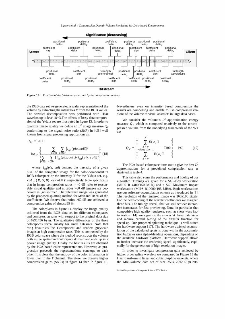
Figure 12 illustrates a fraction of the bitstream as gener-ated by our method. Note, that the number of bits varies as afunction of the individual Huffman codes.
5. Results
To investigate the performance of the proposed method, weapplied the approach to the RGB-Visible Human Dataset ofsize 128x128x128 voxels (3 x 8 bits/voxel). In addition to
Figure 11: Effect of spatial clustering:a) Without clusteringb) With clustering (position threshold: 3, coefficient threshold = 2)c) With clustering (position threshold: 3, coefficient threshold = 4).
wn C m type, ,( )( )n 0 … N, ,=
∆ C m type, ,( )
∆ C m type, ,( ) =
maxn 0 … N 1–, ,=
wn C m type, ,( ) wn 1+ C m type, ,( )–( )
2P----------------------------------------------------------------------------------------------------------------------------------
δ C m type n, , ,( ) =
roundwn C m type, ,( ) wn 1+ C m type, ,( )–( )
∆ C m type, ,( )--------------------------------------------------------------------------------------------------
w̃n C m type, ,( )
n 1 … N, ,=
w̃n 1+ C m type, ,( ) sign n 1+( ) w̃n C m type, ,( )δ C m type n, , ,( ) ∆ C m type, ,( )⋅–
()
=
10
9
78
8
6
52
6
10
9
78
8
6
5
10
9
78
8
6
5
a) b) c)
13
54
1
2
3
4
5
6
2
1
3
4
56
Table 3: Coding schemes:
TAG CODING SCHEMES
SPATIAL POSITIONSPATIAL CLUSTERING, DELTA
CODING, HUFFMAN-TABLE
TYPE RUNLENGTH, HUFFMAN-TABLE
DEPTH RUNLENGTH, HUFFMAN-TABLE
COLOR CHANNEL RUNLENGTH, HUFFMAN-TABLE
SCALAR FACTOR (SIGN) SINGLE BIT
SCALAR FACTOR (VALUE) DELTA CODING, HUFFMAN-TABLE
w0 C m type, ,( )
∆ C m type, ,( )
Lippert et al. / Compression Domain Volume Rendering for Distributed Environments
© 1998 Department of Computer Science, ETH Zurich.
the RGB data set we generated a scalar representation of thevolume by extracting the intensitiesY from the RGB values.The wavelet decomposition was performed with Haarwavelets up to levelM=3.The effects of lossy data compres-sion of the Y-data set are illustrated in figure 13. In order toquantize image quality we define anL2 image measure QIconforming to the signal-noise ratio (SNR) in [dB] wellknown from signal processing applications as:
(18)
where, i im(pix, col) denotes the intensity of a givenpixel of the computed image for thecolor-component inRGB-colorspace or the intensityY for the Y-data set, e.g.
or respectively. Note specificallythat in image compression ratios > 40 dB refer to reason-able visual qualities and at ratios >60 dB images are per-ceived as „noise-free“. The reference image was generatedby the proposed splatting method forM=0 and 100% of thecoefficients. We observe that ratios >60 dB are achieved atcompression gains of almost 95 %.
The colorplates in figure 14 display the image qualityachieved from the RGB data set for different colorspacesand compression rates with respect to the original data sizeof 6291456 bytes. The qualitative differences of the threecolorspaces reveal mostly for small datasizes. Note thatYIQ favourises theY-component and renders greyscaleimages at high compression rates. This is contrasted by theRGB color space where the method reconstructs the volumeboth in the spatial and colorspace domain and ends up in apoorer image quality. Finally the best results are obtainedby the PCA-based color representations. However, as pro-gression proceeds the representations converge to eachother. It is clear that the entropy of the color information islower than in theY channel. Therefore, we observe highercompression gains (SNRs) in figure 14 than in figure 13.
Nevertheless even on intensity based compression theresults are compelling and enable to use compressed ver-sions of the volume as visual abstracts in large data bases.
We consider the volume’sL2 approximation energymeasureQV which is computed relatively to the uncom-pressed volume from the underlying framework of the WTas:
(19)
The PCA-based colorspace turns out to give the bestL2
approximations for a predefined compression rate asdepicted in table 4.
This table also sums the performance and fidelity of ouralgorithm. Timings are given for a SGI-Indy workstation(MIPS R 4400/150 MHz) and a SGI Maximum Impactworkstation (MIPS R10000/195 MHz). Both workstationsuse our software-accumulation scheme as introduced in [9].The resolution of the rendered image was 160x180 pixels.For the delta-coding of the wavelet coefficients we assignedthree bits. The timings reveal, that we still achieve interac-tive framerates for fast previewing. Note, in particular thatcompetitive high quality renderers, such as shear warp fac-torization [14] are significantly slower at these data sizesand require careful setting of the transfer function forspeed-up. Our proposed splatting technique is well-suitedfor hardware support [17]. The hardware assisted accumu-lation of the calculated splats is done within the accumula-tion buffer or uses alpha-blending operations, depending onthe available hardware platform. Hardware support allowsto further increase the rendering speed significantly, espe-cially for the generation of high resolution images.
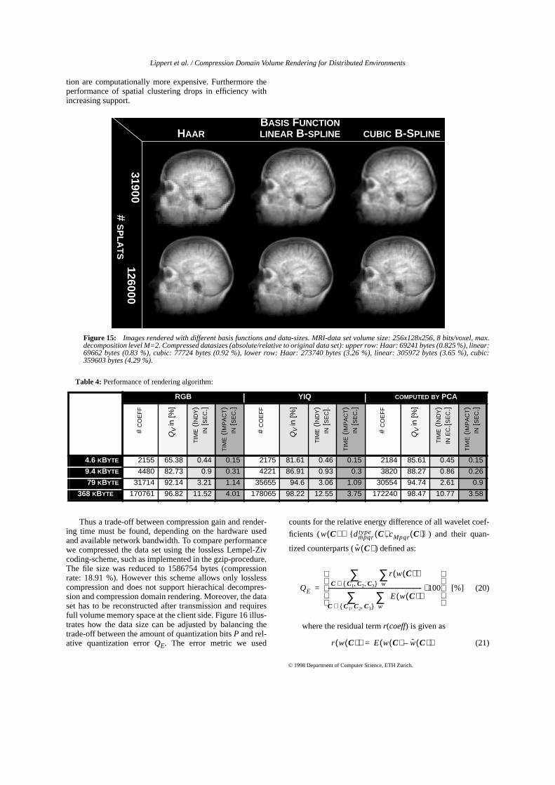
In order to investigate compression gain achieved byhigher order spline wavelets we compared in Figure 15 theHaar transform to linear and cubic B-spline wavelets, wherethe MRI-volume data set of size 256x128x256 (8 bits/
Figure 12: Fraction of the bitstream generated by the compression scheme
positionaldeltax
positionaldeltay
positionaldeltaz
runlengthwavelettype
coefficientdelta
positionaldeltax
positionaldeltaz
coefficientsign
positionaldeltax
positionaldeltay
positionaldeltaz
coefficientdelta
runlengthcolorchannel
positionaldeltax
positionaldeltay
coefficientdelta
positionaldeltay
coefficientdelta
positionaldeltax
positionaldeltaz
01100010010101110010111110111001101111011001111011001110011110111010010011010100101011011111001
Significance (decreasing)
positionaldeltaz
positionaldeltay
coefficientdelta
coefficientsign
coefficientsign
coefficientsign
coefficientsign
Bitstream
Server Client
QI 20 ⋅=
log10
i ref pix col,( )[ ]2
color∑
pixel∑
i im pix col,( ) i ref pix col,( )–[ ]2
color∑
pixel∑
-------------------------------------------------------------------------------------------------------
col R G B, ,{ }∈ col Y≡
QV
E wn( )n 0=
N
∑
E wn( )n 0=
volume size 1–
∑-------------------------------------------- 100⋅
[%]=

Lippert et al. / Compression Domain Volume Rendering for Distributed Environments
© 1998 Department of Computer Science, ETH Zurich.
voxel) is displayed. The wavelet transform was performedup toM=2. The blocky structure of the Haar wavelet clearlyleads to a blocky representation of the data set whereas thehigher order wavelets come up with a smooth, somewhatblurry representation. Obviously, increasing numbers of
vanishing moments lead to higher compression rates. Amajor drawback of higher order wavelets however is theincreasing support which affects the splat size. As a conse-quence both FFT computation and the footprint accumula-
Figure 13: Compression of intensity data set. (data source: Visible Human Project, RGB-data set converted to Y). a) data size: 1496 bytes(rel. data size: 0.07 %), QI = 19.19 dB. b) data size: 3164 bytes (rel. data size: 0.15 %), QI = 31.23 dB. c) data size: 26198 bytes (rel. datasize: 1.25 %), QI = 48.71 dB. d) data size: 122680 bytes (rel. data size: 5.85 %), QI = 61.17 dB.
Figure 14: Progressive compression in three different colorspaces. (data source: Visible Human Project, RGB-data set). Volume size: 1283,max. decomposition level M=3.
a) b) c) d)
RG
Bdf
RG
BC
OM
PU
TE
DB
YP
CA
YIQ
CO
LOR
SP
AC
E
DATA SIZEABS: 4.6 KBYTE ABS: 9.4 KBYTE ABS: 79 KBYTE ABS: 368 KBYTE
QI = 16.22 DB
REL: 0.07 % REL: 0.15 % REL: 1.25 % REL: 5.84 %
QI = 15.24 DB
QI = 31.35 DB
QI = 29.67 DB
QI = 28.65 DB
QI = 46.01 DB
QI = 49.94 DB
QI = 51.29 DB
QI = 62.61 DB
QI = 68.65 DB
QI = 70.71 DBQI = 38.67 DB
Lippert et al. / Compression Domain Volume Rendering for Distributed Environments
© 1998 Department of Computer Science, ETH Zurich.
tion are computationally more expensive. Furthermore theperformance of spatial clustering drops in efficiency withincreasing support.
Thus a trade-off between compression gain and render-ing time must be found, depending on the hardware usedand available network bandwidth. To compare performancewe compressed the data set using the lossless Lempel-Zivcoding-scheme, such as implemented in the gzip-procedure.The file size was reduced to 1586754 bytes (compressionrate: 18.91 %). However this scheme allows only losslesscompression and does not support hierachical decompres-sion and compression domain rendering. Moreover, the dataset has to be reconstructed after transmission and requiresfull volume memory space at the client side. Figure 16 illus-trates how the data size can be adjusted by balancing thetrade-off between the amount of quantization bitsP and rel-ative quantization errorQE. The error metric we used
counts for the relative energy difference of all wavelet coef-
ficients ( ) and their quan-
tized counterparts ( ) defined as:
(20)
where the residual termr(coeff) is given as
(21)
Figure 15: Images rendered with different basis functions and data-sizes. MRI-data set volume size: 256x128x256, 8 bits/voxel, max.decomposition level M=2. Compressed datasizes (absolute/relative to original data set): upper row: Haar: 69241 bytes (0.825 %), linear:69662 bytes (0.83 %), cubic: 77724 bytes (0.92 %), lower row: Haar: 273740 bytes (3.26 %), linear: 305972 bytes (3.65 %), cubic:359603 bytes (4.29 %).
Table 4: Performance of rendering algorithm:
RGB YIQ COMPUTED BY PCA
#C
OE
FF
QV in
[%]
TIM
E(I
ND
Y)
IN[S
EC
.]
TIM
E(I
MP
AC
T)
IN[S
EC
.]
#C
OE
FF
QV in
[%]
TIM
E(I
ND
Y)
IN[S
EC
].
TIM
E(IM
PA
CT)
IN[S
EC
.]
#C
OE
FF
QV in
[%]
TIM
E(I
ND
Y)
INE
C.[S
EC
.]
TIM
E(IM
PA
CT)
IN[S
EC
.]
4.6 KBYTE 2155 65.38 0.44 0.15 2175 81.61 0.46 0.15 2184 85.61 0.45 0.15
9.4 KBYTE 4480 82.73 0.9 0.31 4221 86.91 0.93 0.3 3820 88.27 0.86 0.26
79 KBYTE 31714 92.14 3.21 1.14 35655 94.6 3.06 1.09 30554 94.74 2.61 0.9
368 KBYTE 170761 96.82 11.52 4.01 178065 98.22 12.55 3.75 172240 98.47 10.77 3.58
HAAR LINEAR B-SPLINE CUBIC B-SPLINE
#S
PLA
TS
31900126000
BASIS FUNCTION
w C( ) dmpqrtype C( ) cMpqr C( ){ , }∈
w̃ C( )
QE
r w C( )( )w∑
C C1 C2 C3, ,{ }∈∑
E w C( )( )w∑
C C1 C2 C3, ,{ }∈∑
------------------------------------------------------------------- 100⋅
[%]=
r w C( )( ) E w C( ) w̃ C( )–( )=

Lippert et al. / Compression Domain Volume Rendering for Distributed Environments
© 1998 Department of Computer Science, ETH Zurich.
Figure 16 shows a breakdown of the data size of a givenvolume data set displayed on the right side for an increasingnumber of quantization bits. The total length of each barrepresents the overall data size. Each bar is divided intofractions representing the data sizes for positional data, type
and coefficient-value. Positional data and type are losslessand hence not influenced by the amount of quantizationbits. The figure shows that the data size increases linearlywith the number of bits, whereas the quantization errordecreases exponentially.
6. Conclusions and Future Work
We have presented a method for progressive compressiondomain volume visualization based on a unified waveletdata representation and rendering framework. As an imagebased approach we don‘t need to fully decompress andstore the 3D data set upon rendering. Moreover, the volumecan be rendered immediately from the compressed bitst-ream, which features progressive organization and allows torefine the image according to the provided data. The twoessential featuresprogressionand compressionmake theframework especially suited for networked and distributedenvironments. In particular the limited memory require-ments of our image based method enable to run it even onvery low cost computers. In this context the frameworkoffers flexibility in balancing the trade-off between networkperformance and local computational capabilities of clientand server. In addition, since the performance is mostlydriven by the underlying CPU capabilities we expect anperformance upscaling with each new generation of proces-sors. However, although we proposed some further algo-rithms to enhance visual quality the method is considered asa fast and low quality rendering technique, which can oper-ate as an interactive volume data browser.
At this point in time we are working on a Java-applet[6] for further evaluations. In addition we will examine theusefulness of an arithmetic coding scheme. Since hardware
accumulation boosts the performance significantly, we willprovide an OpenGL interface for 3D PC graphics boards.Furthermore the transmission of selectively refined, view-dependent data over a low-bandwidth network will beinvestigated.
7. Acknowledgments
The authors would like to thank R. Dittrich, A. Eggen-berger, A. Hubeli, J. Pittet, and P. Ruser for implementingparts of the framework. This work was supported by theETH research council under grant No. 41-2642.5.
8. References[1] C. Busch and M. H. Gross. “Interactive neural network
texture analysis and visualization for surface reconstruc-tion in medical imaging.” In R. J. Hubbold and R. Juan,editors, Eurographics ’93, pages 49–60, Oxford, UK,1993. Eurographics, Blackwell Publishers.
[2] B. Cabral, N. Cam, and J. Foran. “Accelerated volume ren-dering and tomographic reconstruction using texture map-ping hardware.” In A. Kaufman and W. Krueger, editors,1994 Symposium on Volume Visualization, pages 91–98.ACM SIGGRAPH, Oct. 1994. ISBN 0-89791-741-3.
[3] C. K. Chui and J. Z. Wang. “A cardinal spline approach towavelets.”Proc. Amer. Math. Soc., 113:785–793, 1991.
[4] R. Crawfis and N. Max. “Direct volume visualization ofthree-dimensional vector fields.”1992 Workshop onVolume Visualization, pages 55–60, 1992.
Figure 16: Relation between data size and number of bits for quantization (data source: Visible Human Project, CT-data set). Volume size:2563, max. decomposition level M=3, no. of splats 74340. a) proportions of coefficient, type and positional data and resulting data size.. b)reference image of compressed data set.
0
20000
40000
60000
80000
100000
120000
140000
160000
180000
200000
2 3 4 5 6 7
position type coefficient
QE in [%]
cumulative data size [bytes]
quantization bits (P) 2 3 4 5 6 7
1.674 0.355 0.0806 0.0217 0.000598 0.000229
a) b)

Lippert et al. / Compression Domain Volume Rendering for Distributed Environments
© 1998 Department of Computer Science, ETH Zurich.
[5] I. Daubechies.Ten Lectures on Wavelets. CBMS-NSFregional conference series in applied mathematics, no.61,SIAM, 1992.
[6] E. E. V. V. Environment). “Homepage.” http://www.inf.ethz.ch/personal/lippert/EVOLVE.
[7] K. Fukunaga.Introduction to Statistical Pattern Recogni-tion. 2nd Ed.. Academic Press, New York, 1990.
[8] M. H. Gross. “L^2 optimal oracles and compression strat-egies for semiorthogonal wavelets.” Technical Report 254,Computer Science Department, ETH Zürich, 1996. http://www.inf.ethz.ch/publications/tr200.html.
[9] M. H. Gross, L. Lippert, R. Dittrich, and S. Häring. “Twomethods for wavelet-based volume rendering.” TechnicalReport 247, ETH-Zürich, 1996.
[10] M. Haley and E. Blake. “Incremental volume renderingusing hierarchical compression.”Computer GraphicsForum, 15(3):44–55, 1996.
[11] G. Held and T. R. Marshall.Data Compression. JohnWiley & Sons Ltd., 1991.
[12] J. T. Kajiya and B. P. Von Herzen. “Ray tracing volumedensities.” In H. Christiansen, editor,Computer Graphics(SIGGRAPH ’84 Proceedings), volume 18, pages 165–174, July 1984.
[13] A. Kaufman.Volume Visualization. IEEE Computer Soci-ety Press, 1990.
[14] P. Lacroute and M. Levoy. “Fast volume rendering using ashear–warp factorization of the viewing transformation.”In A. Glassner, editor,Proceedings of SIGGRAPH ’94(Orlando, Florida, July 24–29, 1994), Computer GraphicsProceedings, Annual Conference Series, pages 451–458.ACM SIGGRAPH, ACM Press, July 1994. ISBN 0-89791-667-0.
[15] D. Laur and P. Hanrahan. “Hierarchical splatting: A pro-gressive refinement algorithm for volume rendering.” InT. W. Sederberg, editor,Computer Graphics (SIGGRAPH’91 Proceedings), volume 25, pages 285–288, July 1991.
[16] M. Levoy. “Display of surfaces from volume data.”IEEEComputer Graphics and Applications, 8(3):29–37, May1988.
[17] L. Lippert and M. H. Gross. “Fast wavelet based volumerendering by accumulation of transparent texture maps.” InProceedings of Eurographics ’95, pages 431–443, 1995.
[18] National Library of Medicine.The Visible Human Project.http://www.nlm.nih.gov/research/visible/visible_human.html, 1995.
[19] D. H. Pritchard. “U.S. color television fundamentals – Areview.” IEEE Transactions on Consumer Electronics,23(4):467–478, Nov. 1977.
[20] E. Quak and N. Weyrich. “Decomposition and reconstruc-tion algorithms for spline wavelets on a bounded inverval.”Applied and Computational Harmonic Analysis, 1(3):217–231, June 1994.
[21] E. J. Stollnitz, T. D. DeRose, and D. Salesin.Wavelets forComputer Graphics. Morgan Kaufmann Publishers, Inc.,1996.
[22] T. Totsuka and M. Levoy. “Frequency domain volumerendering.” In J. T. Kajiya, editor,Computer Graphics(SIGGRAPH ’93 Proceedings), volume 27, pages 271–278, Aug. 1993.
[23] M. V. Wickerhauser.Adapted Wavelet Analysis fromTheory to Software. A. K. Peters, Ltd., 1994.
[24] B. Yeo and B. Liu. “Volume rendering of DCT-basedcompressed 3D scalar data.”IEEE Transactions on Visual-ization and Computer Graphics, 1(1):29–43, Mar. 1995.ISSN 1077-2626.
EUROGRAPHICS ‘98 Tutorial
© 1998 Institute of Scientific Computing, Department of Computer Science, Swiss Fed-eral Institute of Technology (ETH) Zurich, Switzerland.
Compression DomainVolume Rendering for Distributed Environments
L. Lippert, M. H. Gross, C. Kurmann
Department of Computer Science, ETH Zürich
Email: {lippert, grossm, kurmann}@inf.ethz.chWWW: http://www.inf.ethz.ch/department/WR/cg
Abstract
This paper describes a method for volume data compression and rendering which bases on wavelet splats. Theunderlying concept is especially designed for distributed and networked applications, where we assume aremote server to maintain large scale volume data sets, being inspected, browsed through and rendered inter-actively by a local client. Therefore, we encode the server‘s volume data using a newly designed wavelet basedvolume compression method. A local client can render the volumes immediately from the compression domainby using wavelet footprints, a method proposed earlier. In addition, our setup features full progression, wherethe rendered image is refined progressively as data comes in. Furthermore, framerate constraints are consid-ered by controlling the quality of the image both locally and globally depending on the current network band-width or computational capabilities of the client. As a very important aspect of our setup, the client does notneed to provide storage for the volume data and can be implemented in terms of a network application. Theunderlying framework enables to exploit all advantageous properties of the wavelet transform and forms abasis for both sophisticated lossy compression and rendering. Although coming along with simple illuminationand constant exponential decay, the rendering method is especially suited for fast interactive inspection oflarge data sets and can be supported easily by graphics hardware.
Keywords: volume rendering, multiresolution, progressive compression, splatting, wavelets, networks, dis-tributed applications
1. Introduction
Volume rendering, in general, has been a very importantsubfield of research in computer graphics. Since its inven-tion [12], [16], countless algorithms have been proposed,[13], [14], most of which have been designed for providinghigh quality images at low computational efforts. In thiscontext, recent advancements in graphics hardware help toexploit individual capabilities of graphics workstations [2].If real time performance constrains the method and imagequality can be relaxed, so-called splatting methods [15], [4]have proved to provide good results. Here, footprints of avolume primitive are computed in terms of a small pixmaptexture and are superimposed in the framebuffer to carry outthe final image. Introducing hierarchical basis functions,such as wavelets [17], rendering is carried out progressivelyby accumulating scaled and translated versions of self-simi-lar textures.
Unfortunately, most rendering methods introduced sofar relate to local computation environments. The problemsarising with distributed environments and associated com-pression domain rendering has hardly been addressed in theliterature [24], [10]. However, in times of distributed, worldwide information systems and exponentially increasing vol-ume data sets, requirements for rendering such data havechanged. In many application scenarios, such as in medicalimaging and information systems, situations arise, such asdepicted in figure 1.
Often, volume data sets are stored and maintained by adata base server, which can be accessed by one or morelocal clients via a network. One of the fundamental tasks ofvolume rendering is to inspect interactively and to browsethrough the volume data base, where rendering quality canbe relaxed for the sake of real time performance. Moreover,being a low end workstation, the computational power andstorage capacity of the client are limited and the network‘s

Lippert et al. / Compression Domain Volume Rendering for Distributed Environments
© 1998 Department of Computer Science, ETH Zurich.
bandwidth and latency might vary with its traffic load.Obviously, when designing a rendering method for thesepurposes, we have to consider the following issues:
• Progressivity:For enhanced interactivity, the imageshould be refined progressively as data comes infrom the remote server. Image quality must be con-trolled as a function of the network’s load and cli-ent’s hardware setup.
• Compression domains: In order to store and trans-mit large scale volume data sets, compressionschemes have to be employed. In order to avoid fulldecompression, a sophisticated rendering methodshould carry out computations in the compressiondomain at the client side.
• Memory constraints:In particular with upcomingnetwork computers the capabilities of a local clientmight be reduced significantly. Hence, a data repre-sentation and rendering method is required, whichavoids full expansion of the volume in the clientsmemory.
Along these lines, the research presented here aims atproviding a unified framework for data compression andrendering in a distributed environment. Therefore, we firstpropose a progressive volume data compression scheme. Itenables to store both RGB and intensity volume data effi-ciently on the server in terms of a bitstream and allows fasttransmission over the network. To this end, we first decorre-late the RGB volume data and transform the computedintensities in a preprocess by using B-spline wavelets. Thecoefficients and positions are arranged with decreasingimportance and proceed through various steps, such as
quantization, encoding and bit allocation. The compressionpipeline introduced essentially allows a progressive trans-mission, where the information lost can be controlledlocally and globally. Second, the client carries out all ren-dering immediately in the compression domain. That is wedo not need to perform full decompression of the data whileusing wavelet splats [17], [9]. To increase performance andvisual quality of the images, we propose some significantenhancements of the method. Especially, multiview imagescan be carried out at low additional costs and constant expo-nential transfer is incorporated by phase shifts in Fourierdomain.
Our paper is organized as follows: For reasons of read-ability, we briefly review some fundamentals of waveletbased splatting in section 2. In section 3 we describe somesignificant extensions of the rendering method to gainvisual quality, such as multiviews, depth cueing and simpleshading. The proposed compression pipeline is described infull detail in section 4. Results obtained with our setup areillustrated in section 5.
2. Fundamentals of Wavelet Splats
In this section we describe how wavelet splats can bedefined and used for general volume rendering. Therefore,we briefly summarize the mathematical fundamentals ofsplat computation following the approach presented in [9].In addition, a short description of low albedo rendering andwavelets are given. We assume, however, the reader isfamiliar with the mathematics of wavelets.
Figure 1: Volume-rendering in a distributed client/server environment.
volumeDB
data coding / compression
cache
cache
volumedata
Workstation compressed
compressed
compressedvolume data
compressed
interaction
Fileserver ClientsTerminal cluster WAN/LANWAN/LAN
volume data
network computer
workstation / PC
renderer+
renderer
renderer
data image/
compressed
interaction image/
Lippert et al. / Compression Domain Volume Rendering for Distributed Environments
© 1998 Department of Computer Science, ETH Zurich.
2.1. Low Albedo Volume Rendering
Volume rendering can be regarded as a composition of par-ticles that, in addition to their own emission, receive lightfrom surrounding lightsources and reflect these intensitiestowards the observer.
In classic volume rendering, the amount of lightreceived at pointx from directions up to a ray
lengthtL is computed as:
(1)
where q denotes the volume source term andα theopacity function. For an isotropic medium with constantopacity equation (1) reduces to
(2)
In particular note that for we end up in a X-ray-like image.
Especially in those cases, splatting has proved itsusability for fast volume rendering [15]. In contrast to ray-casting, it allows to reduce the computational complexityfor interpolation and integration to a minimum, since thepreprojected footprints of high-order interpolation func-tions can be stored as lookup tables. The projections them-selves can be computed with an accurate quadraturetechnique. Besides hierarchical splats [15], wavelet splat-ting [17] is a sophisticated extension.
2.2. B-spline Wavelets
Since we aim at a unified data representation for both vol-ume data compression and rendering, we use Chui andWang [3] B-spline wavelet bases of orderj. They havemany usefull properties, such as smoothness and vanishingmoments. In addition, analytic expressions for scaling- andwavelet functions and their duals in the frequency- and spa-tial-domain are given. The mother-scaling function of order1 is defined as:
(3)
Compactly supported scaling functions of orderj can begenerated recursively in terms of cardinal B-splines:
(4)
In the frequency-domain the corresponding functionscollapse intosinc-polynomials of type:
(5)
In the upper termf denotes the frequency andi the com-plex operator. Note, that the upper equation is fundamentalfor splat computation in Fourier domain. The semiorthogo-nality of the function system forj > 1 requires duals. For thecase of B-spline wavelets all primary and dual functionshave linear phase. Furthermore, only rational coefficientshave to be used for the fast wavelet transform.
To fully characterize the wavelet transform, we need todetermine the wavelet functions. For the correspondingwavelets we obtain:
(6)
Note, that their support can be computed straightfor-wardly as [0,2j-1]. Wavelets in three dimensions areobtained easily by non-standard tensor-product extensions[5].
Here volume decomposition is carried out with theduals, whereas reconstruction is performed using the pri-mary functions (4), (6). Note furthermore, that implementa-tions of linear time algorithms [20] can be morechallenging, since additional basis transforms might berequired.
2.3. Construction of Wavelet Splats
In wavelet splatting, the renderer computes the projectionsuch as defined in (2). Taking into account the waveletdecomposition levelm up toM and moving the summationoutside the integral, the formulation collapses to:
(7)
where denote the wavelet coefficients of decom-
position levelm at the spatial positionp, q, r and wavelet-type typeand the coefficient of the scaling function
of level M. The computation of the line integrals for a par-ticular view can be accomplished by Fourier projection slic-ing (FPS). It allows to compute accurate projections of anybasis function. This theorem states that the 2D Fouriertransform of a projection of a functionf(x,y,z) onto a givenplane P equals a plane that slices the Fourier transform
parallel toP and intersects the origin.
Since many wavelet types such as B-splines come alongwith closed form representations in the frequency domain,it is straightforward to apply this theorem to get therequired splats. Figure 2 depicts the setting, where aninverse FFT processes the slices to obtain the wavelet splat.
I t L x s, ,( )
I t L x s, ,( ) q x t s⋅+( )e
α x su+( ) ud
0
t
∫–
td
0
tL
∫=
α
I t L x s, ,( ) q x t s⋅+( )e α– ttd
0
tL
∫=
α 0≡
φ 1[ ] x( ) 1 0 x 1<≤0 otherwise
=
φ j[ ] x( )x
j 1–-----------φ j 1–[ ] x( )
j x–j 1–-----------φ j 1–[ ] x 1–( )+=
Φ j[ ] f( ) 1 ei2πf–
–i2πf
-----------------------
j
=
ψ j[ ] x( ) qj k, φ j[ ] 2x k–( )k 0=
3 j 2–
∑=
with qj k,1–( )k
2 j 1–------------- j
l φ 2 j[ ] k 1 l–+( )
l 0=
j
∑=
I ∞ x s, ,( ) dmpqrtype ψmpqr
3 type, x st+( ) td
∞–
∞
∫type 1=
p q r Z∈, ,
7
∑m 1=
M
∑=
cMpqr φMpqr3 x st+( ) td
∞–
∞
∫p q r Z∈, ,
∑+
dmpqrtype
cMpqr
F ω1 ω2 ω3, ,( )

Lippert et al. / Compression Domain Volume Rendering for Distributed Environments
© 1998 Department of Computer Science, ETH Zurich.
The intersection plane spanned byu, v defines the 2DFourier transform of the texture splats
, whereas the
normal vectorn of the plane equals the direction of the pro-jection. The definition of the viewing parameters is figuredout in spherical coordinates (α,β).
Once the renderer builds the viewpoint dependent inte-gral tables, the screen position of the table is calculated,mapped, weighted by the wavelet coefficient and accumu-lated into the framebuffer. Since the basis functions of dif-ferent iteration levelsm differ by dilation, only eightdifferent splats of depthM have to be calculated. All otherfootprints are derived by subsampling in the spirit of amipmap. Correct sampling and optimized data-structures ofthe calculated splats are discussed in [9].
3. Visual Enhancements
We are now in a position to discuss two significant render-ing features which help to improve the visual quality of thegenerated images. In particular, we introduce a method forthe computation of multiviews, being important in manyapplications, such as medical imaging. Exploiting the sym-metry of 3D tensor-product wavelets allows the additionalcosts to be kept sufficiently low. Furthermore, we addressthe problem of exponential transfer functions in Fourierspace. Phase shifts of the wavelet’s FT enable exponentialtransfer to be incorporated and can be used to simulateshading operations on the fly.
3.1. Multiviews
The rendered images, obtained by our splatting approach,lack occlusion. Since this important visual cue is missingfor the calculated X-ray images, depth information is notpresented to the user. One way to overcome this drawbackis the introduction of a multiview arrangement. Here, thevolume is rendered simultaneously from different directionsand presented to the user in a single window. Exploiting thecoherence of different viewing angles given by the symme-try of tensor-product constructions, the basic single-viewsplatting approach can be extended to a multiview rendererwithout computational overhead for splat computation. Werecall that the tensor-product functions are constructed frompermutations of the 1D basis functions and along thex, y andz directions.
Figure 3 exemplifies the idea. The footprint of the basis
function (3D Haar scaling function of level 0,
aligned to the origin) from the first viewing-direction equalsthe footprint from the second and third direction, e.g. thecalculated footprints can be reused for rendering differentviews. Thus, we propose to generate a lookup table for thebasis functions types 1 to 7 to ensure correct footprint cal-culation. A corresponding lookup table is given in Table 1and illustrated in figure 4 for Haar functions respectively.
In order to combine the three footprints for the eightdifferent basis functions, eight textures are calculated forview 1 by the FPS-theorem. The footprint for the basisfunction is equal for view 1 and 2, whereas the splat
of the view 3 is given by the footprint of the function(texture 4) of view 1. The corresponding permutations are
I u v,( ) F ω1 u v,( ) ω2 u v,( ) ω3 u v,( ), ,( )=
Figure 2: Illustration of the Fourier projection slicing theorem in 3D for an idealized Shannon wavelet.
ω1
ω2 slicing plane
Φ ω1 ω2 ω3, ,
u
v
φ x µ ν t, ,( ) y µ ν t, ,( ) z µ ν t, ,( ), ,( )
∞–
∞
∫ dt
ν
µ
slic
ing
iFF
T
frequency domain spatial domain
Φ u v,( )
frequency domain
α
β
u
v
n
ω3
φ ψ
Figure 3: Illustration of the multiview concept.
Table 1: Permutations and negations for multi view arrange-ments
PERMUTATIONS NEGATIONS
VIEW 1 [ 0 1 2 3 4 5 6 7 ] [ 1 1 1 1 1 1 1 1 ]
VIEW 2 [ 0 1 4 5 2 3 6 7 ] [ 1 1 -1 -1 1 1 -1 -1]
VIEW 3 [ 0 4 2 6 1 5 3 7 ] [ 1 1 1 1 -1 -1 -1 -1 ]
y
z
x
view 2
view 1
view
3view 1view 2
view 3φ00003 1[ ]
φ00003 1[ ]
φφψψφφ

Lippert et al. / Compression Domain Volume Rendering for Distributed Environments
© 1998 Department of Computer Science, ETH Zurich.
given for all basis functions and for three views in Table 1.In some cases it is also necessary to multiply the intensitywith -1. The same permutation tables can also be used forhigher order wavelets.
Note that these permutations are equal for each viewingdirection. Note furthermore that the angles between theindividual viewing planes are not constant. Moreover, theydepend on the initial selection of the camera parameters. Alittle algebra reveals that the three projection-planesPi,spanned by the vectors (ui,vi) are given by
View 1: with
View 2: with
View 3: with
The triple view rendering is illustrated in figure 5,where a classified data set is displayed from three direc-tions. The image was grabbed directly from the screen as itis displayed to the user. Skin is colored white, brain tissuered and a tumor is colored in blue.
3.2. Depth Cueing
Up to now, only linear depth cueing has been considered inthe frequency domain [22]. In order to compute constantexponential decay as in (2) we propose a depth cueingapproach implemented as a two step solution. In the firststep the cued footprints have to be calculated by the FPS-theorem and an additional phase-shift. Second, the textureshave to be weighted according to the distance between theprojection plane and the basis functions.
Footprint Computation In order to set up the Fourierrelations for exponentially weighted functions, let’s firstconsider the relations in the spatial domain. Letdenote the function that is depth cued alongt and letk bethe constant exponential extinction coefficient. We obtain
the new function as:
(8)
In the frequency domain the Fourier transform ofcan be written as:
(9)
Obviously, the Fourier transform of the exponentially
depth-cued function is computed by shiftingwith the imaginary frequencyf0. This can be interpreted as
Figure 4: Different wavelet types figured out by non-standardtensor-product extensions for the Haar case.
u1 v1,( )
u1
αsin–
αcos
0
ux
uy
uz
= = v1
αcos– βsin
αsin– βsin
βcos
vx
vy
vz
= =
u2 v2,( )
u2
αcos–
αsin–
0
u– y
ux
uz
= = v2
αsin– βsin
αcos βsin
βcos
v– y
vx
vz
= =
u3 v3,( )
u3
0
αcos
αsin
uz
uy
u– x
= = v3
βcos–
αsin– βsin
αcos βsin
v– z
vy
v– x
= =
++
++
+
+
++
++
+
+ --
--
--
+
+++
--
--
+++
-- -
--
+++
+
++
+
++
++
++
+
+-
--
---
++
---
---
+++
+
+
+ -
--
-
--
-+
+++
--
++
View 1View 2
View 3
Tex5ψφψ Tex6ψψφ Tex7ψψψ
Tex3φψψTex2φψφTex1φφψTex0φφφ
Tex4ψφφ
-
--
---
+
--
+++
Figure 5: Triple views seen from different viewing angles as ap-plied to classified MR-data set (volume size: 256 x 128 x 256, max.decomposition level M = 2) a)α = β = 0.0 b)α = 0.66,β = 0.91.
a) b)
h t( )
h̃ t( )
h̃ t( ) h t( )ekt=
h t( )ei2π f 0t–
where= f 0k2πi–
----------- ki2π------= =
h̃ t( )
H̃ f( ) h̃ t( )ei2πfttd
∞–
∞
∫=
h t( )ei2π f f 0–( )t
td
∞–
∞
∫=
H f f 0–( )=
h̃ t( ) H f( )

Lippert et al. / Compression Domain Volume Rendering for Distributed Environments
© 1998 Department of Computer Science, ETH Zurich.
a “frequency phase shift”. For the B-spline scaling func-tions and wavelets of orderj in the frequency domain wehave
(10)
where
(11)
In 3D the direction of the shift operation in the spec-trum can be chosen without any restriction and indepen-dently from the viewing direction. It corresponds to thedepth-cueing direction in the spatial domain. We define thecueing vectorL for any pair of viewing angles (αl , βl) as
(12)
to determine the cueing direction and extinction coeffi-cient. Figure 6 shows the calculated splats resulting fromthis method.
Distance Weighting For correct depth cueing of the vol-ume, the computed footprints have to be weighted accord-ing to their distance from a reference plane which can beregarded as a planar light source, perpendicular to thedepth-cueing vectorL that points towards the volume mid-point VM. Let L init represent the intersection point of thevolume’s bounding sphere and its tangent plane, the weight-ing factorωd for each basis function centered atBM= P +L init can be computed as:
(13)
During the accumulation process this factor is multi-plied with the wavelet coefficient and the accumulation stepproceeds straightforwardly. The geometric relationships aredepicted in figure 7.
As a result we come up with smooth and correctlydepth-cued volumes, such as shown in figure 6.
To illustrate the performance of our method, we appliedthe approach to the visible human CT-data set [18]. Theinfluence of different factors |k| and different cueing direc-tions are displayed in figure 8 Note that exponential depthcueing increases the rendering performance, since less tex-tures have to be accumulated. Moreover, interactive manip-ulation of the cueing direction allows us to simulate simpleshading operations in the wavelet domain and enhances thevisual quality significantly.
4. Progressive Compression and Transmission
As motivated earlier, our approach is targeted at networkedapplications where, for instance, a local client with lowcomputational power browses through a remote database.Thus, in order to transmit our volume data efficiently wehave to find appropriate compression strategies. It is clearthat the underlying framework of the wavelet decomposi-
Φ̃ j[ ] f( ) 1 ei2π f f 0–( )–
–i2π f f 0–( )
-----------------------------------
j
=
Ψ̃ j[ ] f( ) R j[ ] ei π f f 0–( )–
Φ̃ j[ ] f
2---
=
R j[ ] ei π f f 0–( )–
1
2--- qj n, e
i π f f 0–( )–
n
⋅n ∞–=
∞
∑=
L αl βl,( ) k
αlcos– βlcos
αsin l βlcos
βlsin
kx
ky
kz
= =
ωd e dist–= where distL P⋅
L------------=
Figure 6: Exponentially depth-cued scaling function (j=1) a)|k|=0.0. b) |k|=0.6. Distance weighted footprints: c) depth cuedsplats without distance weighting, d) corrected splats using dis-tance weighting.
Figure 7: Geometric relationships for distance-weighting of ba-sis functions.
t
L
φ
t
L
φ
c) d)
t t
LL
φ φ
a) b)
x
z
y
Ldist
bounding sphereof volume data set
LinitBM
VM
planar light source
P
(tangent plane ofbounding sphere)
Lippert et al. / Compression Domain Volume Rendering for Distributed Environments
© 1998 Department of Computer Science, ETH Zurich.
tion proposes to develop an optimized compression tech-nique that allows progressive transmission, one passdecompression and direct rendering at interactive framerates. Moreover, the wavelet domain rendering avoids fulldecompression of the data prior to the splatting which itselfas an image based method does not require to store the fullvolume data at the client’s side. Although much researchhas been done on wavelet compression methods [21], [23]the specific needs of compression domain renderingencouraged us to develop a new compression pipelinewhich will be explained below. For the sake of brevity werestrict our description to the issues essential for ourmethod and recommend further readings in the fundamen-tals of data compression [11].
4.1. Overview
Figure 9 illustrates the data flow in our compression andrendering setup. The data preprocessing comprises fivestages. It enables both intensity and RGB volumes to behandled, which might be the result of an optional data clas-sification step [1]. In case of RGB volumes the second stepconsists of a colorspace optimization which essentiallydecorrelates the data and allows color sensitive quantiza-tion. Next, a wavelet transform is performed independentlyon the three channels. Lossy compression is carried out byan oracle [8] which operates locally or globally in the wave-let domain. The final step includes a data compression andencoding scheme to achieve a binary output stream that canbe stored locally or transmitted directly through a network.Note that forward compression does not have any real-timeconstraints as opposed to the decompression.
In our implementation the software decompressorworks at a rate of ~30 k wavelet-coefficients/sec. on an IndyR4400 workstation and allows on-line decompression. Therenderer splats the computed footprints weighted with thedecoded wavelet-coefficients directly into a software orhardware accumulation buffer. In addition, our frameworkincorporates a local cache to store coefficients at the client’sside. The required splats are computed locally. Since thewavelet coefficients are transmitted in significance order therendering quality is fully controlled by a user-defined fra-merate, the client’s hardware and, if no cache mechanism isenabled, also by the bandwidth of the network. Hence, this
concept balances CPU, network and graphics performanceand allows scalability. In a minimum configuration we haveto provide client storage only for the eight mother-waveletsplats and three Huffman tables. Together they take lessthan 5KB of memory even for huge data sets. This evenallows the scheme to run on some of the upcoming networkcomputers.
4.2. Colorspace Transformations
If the initial volume is given in RGB, it is critical to trans-form the volume into an optimized colorspace prior to com-pression. Here, we assume the optimized space to bespanned by the three vectorsC1, C2 andC3. This allows toassign an additional significance to each vector. As a resultwe get two independent significance weights per coefficientwhich affect encoding and quantization. The first weight isdefined by the energy of the associated function [8]. Thesecond one is a global significance determined by the color-space-coordinates. For instance, a coefficient with the coor-dinates (1,0,0) is regarded as more relevant than acoefficient (0,1,0) if the vectorC1 is considered to be moresignificant thanC2.
In addition to RGB we employ two colorspaces: Thefirst one is data-independent and equals the YIQ-colorspaceobtained by a simple matrix transform [19]. TheY compo-nent encodes the luminance information, whereas the chro-maticity is encoded inI and Q. We followed the NTSCbandwidth conventions and assigned a factor 4 toY, 1.5 toIand 0.6 toQ. In practical use this colorspace allows to com-pute a black and white image (Y) as a rough sketch and torefine color progressively. Thus, progression is figured outboth in the spatialand in color domain. Alternatively, oursecond colorspace is calculated by a statistically optimalprinciple component analysis (PCA) or Karhunen-Loèveexpansion [7] whose matrix has to be computed individu-ally for each data set. Although the solutions of the eigen-problems are computationally more challenging on offlineforward compression, yet they provide better results (seesection 5). In this case the absolute values of the eigenva-lues are taken to describe the significance of the corre-sponding eigenvector. Note that this step can be skipped forintensity volumes, such as raw CT or MRI data sets.
Figure 8: Influence of different cueing parameters and directions.(data source: Visible Human Project, courtesy National Library of Med-icine, copyright (C) 1995). Volume size: 2563, max. decomposition level M=3. a-c):α = αl = 2.5, β = βl = 0.1, a) |k| = 0, b) |k| = 0.1, c) |k|= 0.2, d)α = 2.5, αl = π/4, β = 0.1,βl = 0.3, |k| = 0.2.
a) b) c) d)

Lippert et al. / Compression Domain Volume Rendering for Distributed Environments
© 1998 Department of Computer Science, ETH Zurich.
4.3. Data Compression Pipeline
The algorithmic steps for data compression are executedsequentially in the pipeline summarized in figure 10 andconvert the wavelet transformed data sets into a sequentialbitstream.
Therefore, we start with a sorting operation that gener-ates a sequence of coefficients and positional data in signif-icance order. The significance scoreS is determined foreach color channel and coefficient
individually according to
its associated wavelet energyE and color channel impor-tance I.
(14)
Table 2 summarizes the importance factors for the threedifferent colorspaces.
For each color channel (C), wavelet type (type) anddecomposition level (m) a deltacoding, normalization andquantization operation is performed separately dependingon the individual ranges of the coefficientsw. More pre-cisely, if quantization is restricted toP bits for a given
Figure 9: Setup for distributed compression domain rendering.
Data Set
R G B
C1
slicing
iFFT
WT
filtering
weighted
accumulation
rendering
transformations
Encoder Decoder
Colorspace optimization
Network
texturemapping
Server Client
classification
Basis Functions
...0011 cache
C2
C3
010010...DB
Figure 10: Pipeline representing the individual steps of the com-pression scheme.
Waveletcoefficients (WC)
deltacoding WC
normalization ∆WC
Huffmancoding runlength
bitstream
runlength-coding
deltacoding Pos
bitstuffing
Huffmancoding ∆WC
Huffmancoding ∆Pos
channel 2channel 1 channel 3
merge-Sort
type, depth, colorchannel
quantization ∆WCC
ompression
Decom
pression
sorting WC
Table 2: Colorspace significance assignment
COLORSPACE IMPORTANCE II(C1) I(C2) I(C3)
RGB 1 1 1
YIQ 4 1.5 0.6
EIGENVECTORS(PCA)
EIGEN-VA-LUE 1
EIGEN-VA-LUE 2
EIGEN-VA-LUE 3
C C1 C2 C3, ,{ }∈
w C( ) dmpqrtype C( ) cMpqr C( ){ , }∈
S w C,( ) E w C( )( ) I C( )⋅=
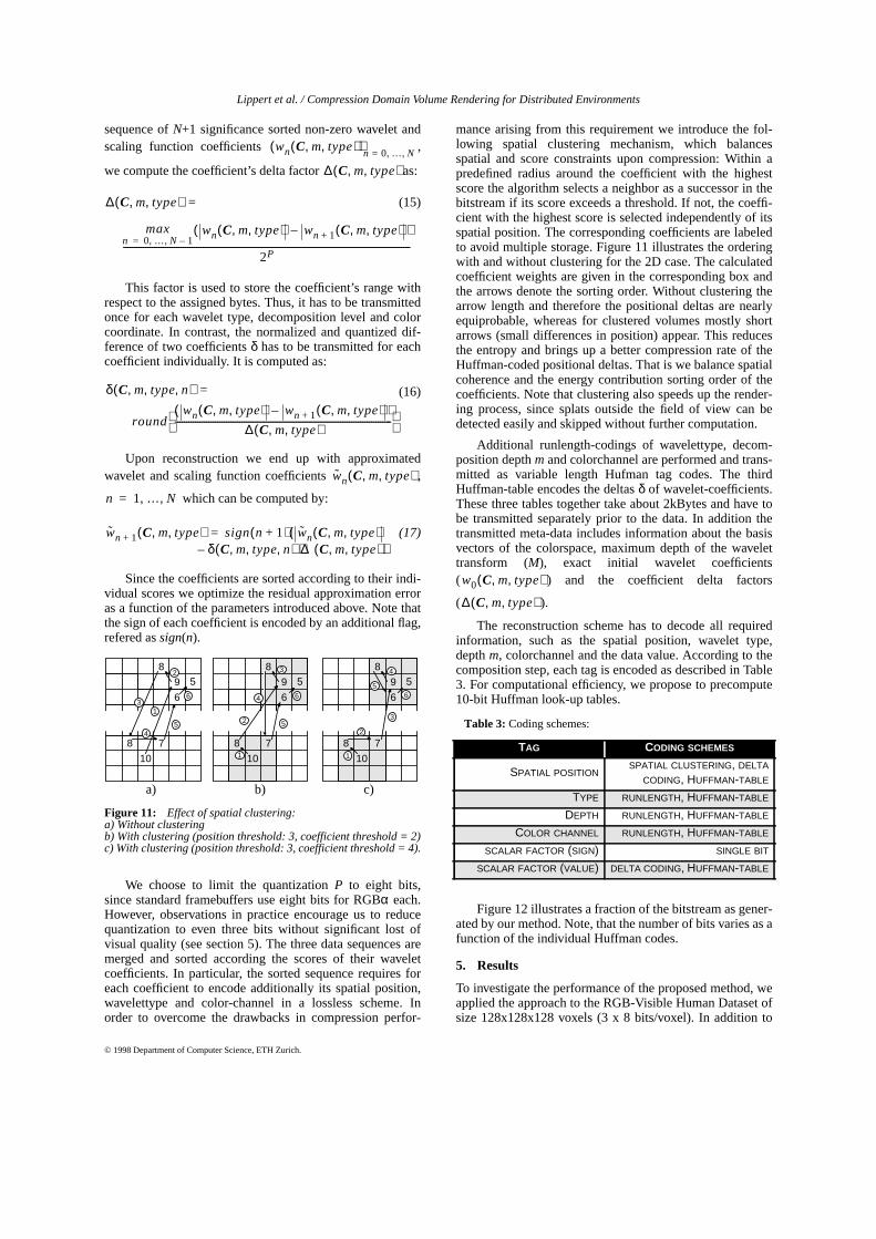
Lippert et al. / Compression Domain Volume Rendering for Distributed Environments
© 1998 Department of Computer Science, ETH Zurich.
sequence ofN+1 significance sorted non-zero wavelet andscaling function coefficients ,
we compute the coefficient’s delta factor as:
(15)
This factor is used to store the coefficient’s range withrespect to the assigned bytes. Thus, it has to be transmittedonce for each wavelet type, decomposition level and colorcoordinate. In contrast, the normalized and quantized dif-ference of two coefficientsδ has to be transmitted for eachcoefficient individually. It is computed as:
(16)
Upon reconstruction we end up with approximatedwavelet and scaling function coefficients ,
which can be computed by:
(17)
Since the coefficients are sorted according to their indi-vidual scores we optimize the residual approximation erroras a function of the parameters introduced above. Note thatthe sign of each coefficient is encoded by an additional flag,refered assign(n).
We choose to limit the quantizationP to eight bits,since standard framebuffers use eight bits for RGBα each.However, observations in practice encourage us to reducequantization to even three bits without significant lost ofvisual quality (see section 5). The three data sequences aremerged and sorted according the scores of their waveletcoefficients. In particular, the sorted sequence requires foreach coefficient to encode additionally its spatial position,wavelettype and color-channel in a lossless scheme. Inorder to overcome the drawbacks in compression perfor-
mance arising from this requirement we introduce the fol-lowing spatial clustering mechanism, which balancesspatial and score constraints upon compression: Within apredefined radius around the coefficient with the highestscore the algorithm selects a neighbor as a successor in thebitstream if its score exceeds a threshold. If not, the coeffi-cient with the highest score is selected independently of itsspatial position. The corresponding coefficients are labeledto avoid multiple storage. Figure 11 illustrates the orderingwith and without clustering for the 2D case. The calculatedcoefficient weights are given in the corresponding box andthe arrows denote the sorting order. Without clustering thearrow length and therefore the positional deltas are nearlyequiprobable, whereas for clustered volumes mostly shortarrows (small differences in position) appear. This reducesthe entropy and brings up a better compression rate of theHuffman-coded positional deltas. That is we balance spatialcoherence and the energy contribution sorting order of thecoefficients. Note that clustering also speeds up the render-ing process, since splats outside the field of view can bedetected easily and skipped without further computation.
Additional runlength-codings of wavelettype, decom-position depthmand colorchannel are performed and trans-mitted as variable length Hufman tag codes. The thirdHuffman-table encodes the deltasδ of wavelet-coefficients.These three tables together take about 2kBytes and have tobe transmitted separately prior to the data. In addition thetransmitted meta-data includes information about the basisvectors of the colorspace, maximum depth of the wavelettransform (M), exact initial wavelet coefficients( ) and the coefficient delta factors
( ).
The reconstruction scheme has to decode all requiredinformation, such as the spatial position, wavelet type,depthm, colorchannel and the data value. According to thecomposition step, each tag is encoded as described in Table3. For computational efficiency, we propose to precompute10-bit Huffman look-up tables.
Figure 12 illustrates a fraction of the bitstream as gener-ated by our method. Note, that the number of bits varies as afunction of the individual Huffman codes.
5. Results
To investigate the performance of the proposed method, weapplied the approach to the RGB-Visible Human Dataset ofsize 128x128x128 voxels (3 x 8 bits/voxel). In addition to
Figure 11: Effect of spatial clustering:a) Without clusteringb) With clustering (position threshold: 3, coefficient threshold = 2)c) With clustering (position threshold: 3, coefficient threshold = 4).
wn C m type, ,( )( )n 0 … N, ,=
∆ C m type, ,( )
∆ C m type, ,( ) =
maxn 0 … N 1–, ,=
wn C m type, ,( ) wn 1+ C m type, ,( )–( )
2P----------------------------------------------------------------------------------------------------------------------------------
δ C m type n, , ,( ) =
roundwn C m type, ,( ) wn 1+ C m type, ,( )–( )
∆ C m type, ,( )--------------------------------------------------------------------------------------------------
w̃n C m type, ,( )
n 1 … N, ,=
w̃n 1+ C m type, ,( ) sign n 1+( ) w̃n C m type, ,( )δ C m type n, , ,( ) ∆ C m type, ,( )⋅–
()
=
10
9
78
8
6
52
6
10
9
78
8
6
5
10
9
78
8
6
5
a) b) c)
13
54
1
2
3
4
5
6
2
1
3
4
56
Table 3: Coding schemes:
TAG CODING SCHEMES
SPATIAL POSITIONSPATIAL CLUSTERING, DELTA
CODING, HUFFMAN-TABLE
TYPE RUNLENGTH, HUFFMAN-TABLE
DEPTH RUNLENGTH, HUFFMAN-TABLE
COLOR CHANNEL RUNLENGTH, HUFFMAN-TABLE
SCALAR FACTOR (SIGN) SINGLE BIT
SCALAR FACTOR (VALUE) DELTA CODING, HUFFMAN-TABLE
w0 C m type, ,( )
∆ C m type, ,( )

Lippert et al. / Compression Domain Volume Rendering for Distributed Environments
© 1998 Department of Computer Science, ETH Zurich.
the RGB data set we generated a scalar representation of thevolume by extracting the intensitiesY from the RGB values.The wavelet decomposition was performed with Haarwavelets up to levelM=3.The effects of lossy data compres-sion of the Y-data set are illustrated in figure 13. In order toquantize image quality we define anL2 image measure QIconforming to the signal-noise ratio (SNR) in [dB] wellknown from signal processing applications as:
(18)
where, i im(pix, col) denotes the intensity of a givenpixel of the computed image for thecolor-component inRGB-colorspace or the intensityY for the Y-data set, e.g.
or respectively. Note specificallythat in image compression ratios > 40 dB refer to reason-able visual qualities and at ratios >60 dB images are per-ceived as „noise-free“. The reference image was generatedby the proposed splatting method forM=0 and 100% of thecoefficients. We observe that ratios >60 dB are achieved atcompression gains of almost 95 %.
The colorplates in figure 14 display the image qualityachieved from the RGB data set for different colorspacesand compression rates with respect to the original data sizeof 6291456 bytes. The qualitative differences of the threecolorspaces reveal mostly for small datasizes. Note thatYIQ favourises theY-component and renders greyscaleimages at high compression rates. This is contrasted by theRGB color space where the method reconstructs the volumeboth in the spatial and colorspace domain and ends up in apoorer image quality. Finally the best results are obtainedby the PCA-based color representations. However, as pro-gression proceeds the representations converge to eachother. It is clear that the entropy of the color information islower than in theY channel. Therefore, we observe highercompression gains (SNRs) in figure 14 than in figure 13.
Nevertheless even on intensity based compression theresults are compelling and enable to use compressed ver-sions of the volume as visual abstracts in large data bases.
We consider the volume’sL2 approximation energymeasureQV which is computed relatively to the uncom-pressed volume from the underlying framework of the WTas:
(19)
The PCA-based colorspace turns out to give the bestL2
approximations for a predefined compression rate asdepicted in table 4.
This table also sums the performance and fidelity of ouralgorithm. Timings are given for a SGI-Indy workstation(MIPS R 4400/150 MHz) and a SGI Maximum Impactworkstation (MIPS R10000/195 MHz). Both workstationsuse our software-accumulation scheme as introduced in [9].The resolution of the rendered image was 160x180 pixels.For the delta-coding of the wavelet coefficients we assignedthree bits. The timings reveal, that we still achieve interac-tive framerates for fast previewing. Note, in particular thatcompetitive high quality renderers, such as shear warp fac-torization [14] are significantly slower at these data sizesand require careful setting of the transfer function forspeed-up. Our proposed splatting technique is well-suitedfor hardware support [17]. The hardware assisted accumu-lation of the calculated splats is done within the accumula-tion buffer or uses alpha-blending operations, depending onthe available hardware platform. Hardware support allowsto further increase the rendering speed significantly, espe-cially for the generation of high resolution images.
In order to investigate compression gain achieved byhigher order spline wavelets we compared in Figure 15 theHaar transform to linear and cubic B-spline wavelets, wherethe MRI-volume data set of size 256x128x256 (8 bits/
Figure 12: Fraction of the bitstream generated by the compression scheme
positionaldeltax
positionaldeltay
positionaldeltaz
runlengthwavelettype
coefficientdelta
positionaldeltax
positionaldeltaz
coefficientsign
positionaldeltax
positionaldeltay
positionaldeltaz
coefficientdelta
runlengthcolorchannel
positionaldeltax
positionaldeltay
coefficientdelta
positionaldeltay
coefficientdelta
positionaldeltax
positionaldeltaz
01100010010101110010111110111001101111011001111011001110011110111010010011010100101011011111001
Significance (decreasing)
positionaldeltaz
positionaldeltay
coefficientdelta
coefficientsign
coefficientsign
coefficientsign
coefficientsign
Bitstream
Server Client
QI 20 ⋅=
log10
i ref pix col,( )[ ]2
color∑
pixel∑
i im pix col,( ) i ref pix col,( )–[ ]2
color∑
pixel∑
-------------------------------------------------------------------------------------------------------
col R G B, ,{ }∈ col Y≡
QV
E wn( )n 0=
N
∑
E wn( )n 0=
volume size 1–
∑-------------------------------------------- 100⋅
[%]=
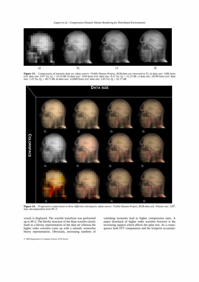
Lippert et al. / Compression Domain Volume Rendering for Distributed Environments
© 1998 Department of Computer Science, ETH Zurich.
voxel) is displayed. The wavelet transform was performedup toM=2. The blocky structure of the Haar wavelet clearlyleads to a blocky representation of the data set whereas thehigher order wavelets come up with a smooth, somewhatblurry representation. Obviously, increasing numbers of
vanishing moments lead to higher compression rates. Amajor drawback of higher order wavelets however is theincreasing support which affects the splat size. As a conse-quence both FFT computation and the footprint accumula-
Figure 13: Compression of intensity data set. (data source: Visible Human Project, RGB-data set converted to Y). a) data size: 1496 bytes(rel. data size: 0.07 %), QI = 19.19 dB. b) data size: 3164 bytes (rel. data size: 0.15 %), QI = 31.23 dB. c) data size: 26198 bytes (rel. datasize: 1.25 %), QI = 48.71 dB. d) data size: 122680 bytes (rel. data size: 5.85 %), QI = 61.17 dB.
Figure 14: Progressive compression in three different colorspaces. (data source: Visible Human Project, RGB-data set). Volume size: 1283,max. decomposition level M=3.
a) b) c) d)
RG
Bdf
RG
BC
OM
PU
TE
DB
YP
CA
YIQ
CO
LOR
SP
AC
E
DATA SIZEABS: 4.6 KBYTE ABS: 9.4 KBYTE ABS: 79 KBYTE ABS: 368 KBYTE
QI = 16.22 DB
REL: 0.07 % REL: 0.15 % REL: 1.25 % REL: 5.84 %
QI = 15.24 DB
QI = 31.35 DB
QI = 29.67 DB
QI = 28.65 DB
QI = 46.01 DB
QI = 49.94 DB
QI = 51.29 DB
QI = 62.61 DB
QI = 68.65 DB
QI = 70.71 DBQI = 38.67 DB

Lippert et al. / Compression Domain Volume Rendering for Distributed Environments
© 1998 Department of Computer Science, ETH Zurich.
tion are computationally more expensive. Furthermore theperformance of spatial clustering drops in efficiency withincreasing support.
Thus a trade-off between compression gain and render-ing time must be found, depending on the hardware usedand available network bandwidth. To compare performancewe compressed the data set using the lossless Lempel-Zivcoding-scheme, such as implemented in the gzip-procedure.The file size was reduced to 1586754 bytes (compressionrate: 18.91 %). However this scheme allows only losslesscompression and does not support hierachical decompres-sion and compression domain rendering. Moreover, the dataset has to be reconstructed after transmission and requiresfull volume memory space at the client side. Figure 16 illus-trates how the data size can be adjusted by balancing thetrade-off between the amount of quantization bitsP and rel-ative quantization errorQE. The error metric we used
counts for the relative energy difference of all wavelet coef-
ficients ( ) and their quan-
tized counterparts ( ) defined as:
(20)
where the residual termr(coeff) is given as
(21)
Figure 15: Images rendered with different basis functions and data-sizes. MRI-data set volume size: 256x128x256, 8 bits/voxel, max.decomposition level M=2. Compressed datasizes (absolute/relative to original data set): upper row: Haar: 69241 bytes (0.825 %), linear:69662 bytes (0.83 %), cubic: 77724 bytes (0.92 %), lower row: Haar: 273740 bytes (3.26 %), linear: 305972 bytes (3.65 %), cubic:359603 bytes (4.29 %).
Table 4: Performance of rendering algorithm:
RGB YIQ COMPUTED BY PCA
#C
OE
FF
QV in
[%]
TIM
E(I
ND
Y)
IN[S
EC
.]
TIM
E(I
MP
AC
T)
IN[S
EC
.]
#C
OE
FF
QV in
[%]
TIM
E(I
ND
Y)
IN[S
EC
].
TIM
E(IM
PA
CT)
IN[S
EC
.]
#C
OE
FF
QV in
[%]
TIM
E(I
ND
Y)
INE
C.[S
EC
.]
TIM
E(IM
PA
CT)
IN[S
EC
.]
4.6 KBYTE 2155 65.38 0.44 0.15 2175 81.61 0.46 0.15 2184 85.61 0.45 0.15
9.4 KBYTE 4480 82.73 0.9 0.31 4221 86.91 0.93 0.3 3820 88.27 0.86 0.26
79 KBYTE 31714 92.14 3.21 1.14 35655 94.6 3.06 1.09 30554 94.74 2.61 0.9
368 KBYTE 170761 96.82 11.52 4.01 178065 98.22 12.55 3.75 172240 98.47 10.77 3.58
HAAR LINEAR B-SPLINE CUBIC B-SPLINE
#S
PLA
TS
31900126000
BASIS FUNCTION
w C( ) dmpqrtype C( ) cMpqr C( ){ , }∈
w̃ C( )
QE
r w C( )( )w∑
C C1 C2 C3, ,{ }∈∑
E w C( )( )w∑
C C1 C2 C3, ,{ }∈∑
------------------------------------------------------------------- 100⋅
[%]=
r w C( )( ) E w C( ) w̃ C( )–( )=
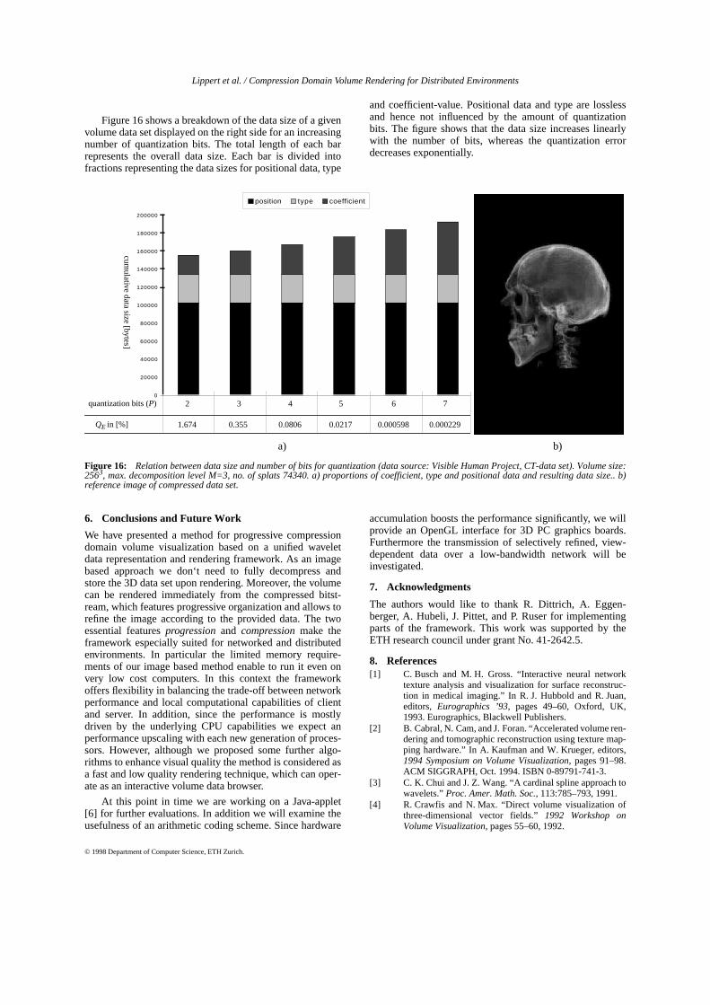
Lippert et al. / Compression Domain Volume Rendering for Distributed Environments
© 1998 Department of Computer Science, ETH Zurich.
Figure 16 shows a breakdown of the data size of a givenvolume data set displayed on the right side for an increasingnumber of quantization bits. The total length of each barrepresents the overall data size. Each bar is divided intofractions representing the data sizes for positional data, type
and coefficient-value. Positional data and type are losslessand hence not influenced by the amount of quantizationbits. The figure shows that the data size increases linearlywith the number of bits, whereas the quantization errordecreases exponentially.
6. Conclusions and Future Work
We have presented a method for progressive compressiondomain volume visualization based on a unified waveletdata representation and rendering framework. As an imagebased approach we don‘t need to fully decompress andstore the 3D data set upon rendering. Moreover, the volumecan be rendered immediately from the compressed bitst-ream, which features progressive organization and allows torefine the image according to the provided data. The twoessential featuresprogressionand compressionmake theframework especially suited for networked and distributedenvironments. In particular the limited memory require-ments of our image based method enable to run it even onvery low cost computers. In this context the frameworkoffers flexibility in balancing the trade-off between networkperformance and local computational capabilities of clientand server. In addition, since the performance is mostlydriven by the underlying CPU capabilities we expect anperformance upscaling with each new generation of proces-sors. However, although we proposed some further algo-rithms to enhance visual quality the method is considered asa fast and low quality rendering technique, which can oper-ate as an interactive volume data browser.
At this point in time we are working on a Java-applet[6] for further evaluations. In addition we will examine theusefulness of an arithmetic coding scheme. Since hardware
accumulation boosts the performance significantly, we willprovide an OpenGL interface for 3D PC graphics boards.Furthermore the transmission of selectively refined, view-dependent data over a low-bandwidth network will beinvestigated.
7. Acknowledgments
The authors would like to thank R. Dittrich, A. Eggen-berger, A. Hubeli, J. Pittet, and P. Ruser for implementingparts of the framework. This work was supported by theETH research council under grant No. 41-2642.5.
8. References[1] C. Busch and M. H. Gross. “Interactive neural network
texture analysis and visualization for surface reconstruc-tion in medical imaging.” In R. J. Hubbold and R. Juan,editors, Eurographics ’93, pages 49–60, Oxford, UK,1993. Eurographics, Blackwell Publishers.
[2] B. Cabral, N. Cam, and J. Foran. “Accelerated volume ren-dering and tomographic reconstruction using texture map-ping hardware.” In A. Kaufman and W. Krueger, editors,1994 Symposium on Volume Visualization, pages 91–98.ACM SIGGRAPH, Oct. 1994. ISBN 0-89791-741-3.
[3] C. K. Chui and J. Z. Wang. “A cardinal spline approach towavelets.”Proc. Amer. Math. Soc., 113:785–793, 1991.
[4] R. Crawfis and N. Max. “Direct volume visualization ofthree-dimensional vector fields.”1992 Workshop onVolume Visualization, pages 55–60, 1992.
Figure 16: Relation between data size and number of bits for quantization (data source: Visible Human Project, CT-data set). Volume size:2563, max. decomposition level M=3, no. of splats 74340. a) proportions of coefficient, type and positional data and resulting data size.. b)reference image of compressed data set.
0
20000
40000
60000
80000
100000
120000
140000
160000
180000
200000
2 3 4 5 6 7
position type coefficient
QE in [%]
cumulative data size [bytes]
quantization bits (P) 2 3 4 5 6 7
1.674 0.355 0.0806 0.0217 0.000598 0.000229
a) b)
Lippert et al. / Compression Domain Volume Rendering for Distributed Environments
© 1998 Department of Computer Science, ETH Zurich.
[5] I. Daubechies.Ten Lectures on Wavelets. CBMS-NSFregional conference series in applied mathematics, no.61,SIAM, 1992.
[6] E. E. V. V. Environment). “Homepage.” http://www.inf.ethz.ch/personal/lippert/EVOLVE.
[7] K. Fukunaga.Introduction to Statistical Pattern Recogni-tion. 2nd Ed.. Academic Press, New York, 1990.
[8] M. H. Gross. “L^2 optimal oracles and compression strat-egies for semiorthogonal wavelets.” Technical Report 254,Computer Science Department, ETH Zürich, 1996. http://www.inf.ethz.ch/publications/tr200.html.
[9] M. H. Gross, L. Lippert, R. Dittrich, and S. Häring. “Twomethods for wavelet-based volume rendering.” TechnicalReport 247, ETH-Zürich, 1996.
[10] M. Haley and E. Blake. “Incremental volume renderingusing hierarchical compression.”Computer GraphicsForum, 15(3):44–55, 1996.
[11] G. Held and T. R. Marshall.Data Compression. JohnWiley & Sons Ltd., 1991.
[12] J. T. Kajiya and B. P. Von Herzen. “Ray tracing volumedensities.” In H. Christiansen, editor,Computer Graphics(SIGGRAPH ’84 Proceedings), volume 18, pages 165–174, July 1984.
[13] A. Kaufman.Volume Visualization. IEEE Computer Soci-ety Press, 1990.
[14] P. Lacroute and M. Levoy. “Fast volume rendering using ashear–warp factorization of the viewing transformation.”In A. Glassner, editor,Proceedings of SIGGRAPH ’94(Orlando, Florida, July 24–29, 1994), Computer GraphicsProceedings, Annual Conference Series, pages 451–458.ACM SIGGRAPH, ACM Press, July 1994. ISBN 0-89791-667-0.
[15] D. Laur and P. Hanrahan. “Hierarchical splatting: A pro-gressive refinement algorithm for volume rendering.” InT. W. Sederberg, editor,Computer Graphics (SIGGRAPH’91 Proceedings), volume 25, pages 285–288, July 1991.
[16] M. Levoy. “Display of surfaces from volume data.”IEEEComputer Graphics and Applications, 8(3):29–37, May1988.
[17] L. Lippert and M. H. Gross. “Fast wavelet based volumerendering by accumulation of transparent texture maps.” InProceedings of Eurographics ’95, pages 431–443, 1995.
[18] National Library of Medicine.The Visible Human Project.http://www.nlm.nih.gov/research/visible/visible_human.html, 1995.
[19] D. H. Pritchard. “U.S. color television fundamentals – Areview.” IEEE Transactions on Consumer Electronics,23(4):467–478, Nov. 1977.
[20] E. Quak and N. Weyrich. “Decomposition and reconstruc-tion algorithms for spline wavelets on a bounded inverval.”Applied and Computational Harmonic Analysis, 1(3):217–231, June 1994.
[21] E. J. Stollnitz, T. D. DeRose, and D. Salesin.Wavelets forComputer Graphics. Morgan Kaufmann Publishers, Inc.,1996.
[22] T. Totsuka and M. Levoy. “Frequency domain volumerendering.” In J. T. Kajiya, editor,Computer Graphics(SIGGRAPH ’93 Proceedings), volume 27, pages 271–278, Aug. 1993.
[23] M. V. Wickerhauser.Adapted Wavelet Analysis fromTheory to Software. A. K. Peters, Ltd., 1994.
[24] B. Yeo and B. Liu. “Volume rendering of DCT-basedcompressed 3D scalar data.”IEEE Transactions on Visual-ization and Computer Graphics, 1(1):29–43, Mar. 1995.ISSN 1077-2626.