Compositional Reasoning for ProbabilisticFinite-State Behaviors

Yuxin Deng1 ?, Catuscia Palamidessi2 ??, and Jun Pang2

1 INRIA Sophia-Antipolis and Universite Paris 7, France2 INRIA Futurs and LIX, Ecole Polytechnique, France

Abstract. We study a process algebra which combines both nondeter-ministic and probabilistic behavior in the style of Segala and Lynch’s sim-ple probabilistic automata. We consider strong bisimulation and observa-tional equivalence, and provide complete axiomatizations for a languagethat includes a restricted form of parallel composition and (guarded)recursion. The presence of the parallel composition, in particular, intro-duces various technical difficulties, but we believe that a “good” com-positional semantics should take it into account since it is an essentialoperator to specify concurrent systems.

1 Introduction

Process algebras, also known as process calculi, are a powerful mathematicalmodel for the specification and verification of concurrent systems. They providea formal apparatus for representing and reasoning about the behaviors of dis-tributed systems, algorithms and protocols in a compositional way. Some of themost prominent representants of these formalisms are CCS [26], ACP [8, 6], andCSP [21].

The axiomatic theories of process algebra provide an elegant way for provingproperties of systems. Both a system and its desired external behavior can beexpressed as process terms. The correctness of the system can then be verifiedby proving that these two terms are equivalent.

In a process algebra typically there are only a few operators, such as actionprefix, summation (nondeterministic choice), recursion and parallel composition.The latter is particularly important for concurrency, as it allows to specify thestructural properties of systems composed of several interacting parts. For exam-ple, a typical communication protocol for data transferring involves two agentsS and R, representing the sender and the receiver, and two lossy channels Kand L between them (see Figure 1). The behavior of each of these four compo-nents can be described as a process term in a chosen process algebra, and thenthey are all put together in parallel to form the complete view of the protocol.The parallel composition operator captures both the interleaving behaviors and? Supported by the EU project PROFUNDIS.

?? Partially supported by the projet Rossignol of the ACI Securite Informatique (Min-istere de la recherche et nouvelles technologies).

S

K

L

R

Fig. 1. A communication protocol

the possible synchronization of the components. The external behavior of theprotocol can be specified as a FIFO queue. The equivalence proof between theprotocol and its external behavior is established by equational reasoning basedon axiomatization, hiding internal behavior, using fairness assumption, and theother feasible methods (see e.g. [9, 17]).

Developing a both complete and sound axiomatization for a chosen bisimu-lation relation over a process algebra expressing finite-state processes has been aresearch focus for the process algebra community. This led to a wealth of classicalresults in the literature. Milner [25, 27] gave complete axiomatizations of bothstrong bisimilarity and observational equivalence for a core CCS (not containingthe parallel composition operator) with both unguarded and guarded recursion.Bergstra and Klop [10] axiomatized observational equivalence in an alternativeway by using an interesting graph rewriting technique. Hennessy and Milner [20]offered a complete equational axiomatization of strong bisimulation over the re-cursion free fragment of CCS. To deal with parallel composition, they used theso-called expansion law, which is an equation schema with a countably infinitenumber of instances. Bergstra and Klop [8] gave a finite equational axiomati-zation of the merge operator (as the parallel composition in CCS) using theauxiliary left merge and communication merge operators. An interesting essayon equational axiomatizations of parallel composition can be found in [2].

Having both recursion and parallel composition in a process algebra compli-cates the matters to establish a complete axiomatization, mostly because thiscan give rise to infinite-state systems even with the guardedness condition. Forexample, let E be the expression µX(a.(X | b)), then we have the infinite transi-tion graph starting from E in Figure 2. Milner pointed out in [27] that in order tohave a complete axiomatization for CCS with both recursion and parallel com-position, a sufficient condition is that the parallel composition does not occur inthe body of any recursive expression.

In this paper we relax this restriction by requiring, instead, that free vari-ables do not appear in the scope of parallel composition. A similar restriction wasadopted, independently, in [5]. In that paper, Baeten and Bravetti considered ageneric process algebra of which CCS, CSP and ACP are subalgebras. Finite-stateness is achieved by requiring that recursion variables do not occur in thescope of static operators, which include the parallel composition. Our work and

2

E . . .

a

E | b E | b | b

a a

b bb

Fig. 2. The transition graph of E.

[5] are, in a sense, incomparable, because we consider a probabilistic and nonde-terministic framework (as explained in the rest of this introduction) with CCS-like communication, while [5] considers a purely nondeterministic paradigm, butmore general than our nondeterministic fragment. The same restriction alreadyappeared in [11], for a nondeterministic process algebra with CSP multiwaysynchronization.

Recently there has been an increasing interest in the area of formal meth-ods for the specification and analysis of probabilistic behaviors, as exhibitedfor instance in randomized, distributed and fault-tolerant systems. The notionof probabilistic bisimulation is introduced first by Larsen and Skou [22]. Latermany variant behavioural equivalences have been defined for various probabilisticmodels. A representative model for analyzing probabilistic systems is providedby Segala and Lynch’s simple probabilistic automata [29], which take into ac-count both probabilistic and nondeterministic behavior and which have beensuccessfully adopted in the studies of distributed algorithms [23, 28] and prac-tical communication protocols [32]. An axiomatization for the finite sequentialfragment of simple probabilistic automata has been provided by Bandini andSegala in [7]. Following this line of research, Deng and Palamidessi [16, 15] havegiven a sound and complete axiomatization for a larger language, which includesthe recursion operator.

In this paper, we improve on [16, 15] by considering also the parallel com-position. To our knowledge, it is the first time that an axiomatization for aprobabilistic and nondeterministic process algebra with both recursion and par-allel operator has been attempted. Similar to the case of classical process algebra,once we have both parallel composition and recursion, the equational axiomati-zation of strong bisimulation and observational equivalence turns out to be quitecomplicated to achieve.

To obtain the completeness of the axiomatizations, we develop a probabilisticversion of the expansion law to eliminate all occurrences of parallel composition.In order to do that, we heavily rely on the condition that only closed terms areput in parallel (cf. Theorem 3).

Concerning soundness, it turns out to be particularly difficult to prove thatstrong and weak bisimilarities are closed under the parallel composition opera-tor. Our approach is to manipulate equivalences of distributions on terms. Animportant property that we exploit in our proofs is Lemma 2, which says thatif two distributions are equivalent with respect to an equivalence relation R,

3

then there is a uniform way to extend them so that the resulting distributionsin parallel contexts are equivalent with respect to another equivalence relationR|. It turns out that if R is instantiated as strong or weak bisimilarity then R|

is a subset of R, thus R| also relates bisimilar expressions.

Structure of the paper. In the next section we briefly recall some basic con-cepts and definitions about probabilistic distributions. In Section 3, we presentthe syntax and operational semantics of a probabilistic process calculus. Next,we give the notions of strong and weak behavioral equivalences in Section 4.We provide complete axiomatizations for strong bisimilarity and observationalequivalence in Sections 5 and 6 respectively, restricted to guarded expressionsin the second case. In Section 7, we conclude and discuss some related work notyet mentioned in the introduction. Detailed proofs of the main propositions inSection 4 are in the Appendix.

2 Preliminaries

Let S be a set. A function η : S 7→ [0, 1] is called a discrete probability distribu-tion, or distribution for short, on S if the support of η, defined as spt(η) = {x ∈S | η(x) > 0}, is finite or countably infinite and

∑x∈S η(x) = 1. We denote by

P(S) the set of distributions over S. If η is a distribution with finite supportand V ⊆ spt(η) we use the set {si : η(si)}si∈V to enumerate the probabilityassociated with each element of V . The constructor ] on this kind of sets isdefined as follows.

{si : pi}i∈I ] {s : p} ={{si : pi}i∈I\j ∪ {sj : (pj + p)} if s = sj for some j ∈ I{si : pi}i∈I ∪ {s : p} otherwise.

{si : pi}i∈I ] {tj : pj}j∈1..n =({si : pi}i∈I ] {t1 : p1}) ] {tj : pj}j∈2..n

Given some distributions η1, ..., ηn on S and some real numbers r1, ..., rn ∈[0, 1] with

∑i∈1..n ri = 1, we define the convex combination r1η1 + ... + rnηn

of η1, ..., ηn to be the distribution η such that η(s) =∑

i∈1..n riηi(s), for eachs ∈ S.

A simple probabilistic automaton is a tuple (S, s, Σ, T ), where S is a set ofstates, s ∈ S is a start state, Σ is a set of actions, and T ⊆ S × Σ × P(S)is a transition relation. Informally, a simple probabilistic automaton is like anordinary automaton except that a labeled transition leads to a probabilisticdistribution over a set of states instead of a single state. Simple probabilisticautomata are used in this paper to give operational semantics of our probabilisticprocess calculus.

3 Probabilistic process calculus

We assume a countable set of variables, Var = {X, Y, ...}, and a countable set ofatomic actions, A = {a, b, ...}. Given a special action τ not in A, we let u, v, ...

4

range over the set of actions, Act = A∪A∪ {τ}, and let α, β, ... range over theset Var ∪Act . The class of expressions E is defined by the following syntax:

E,F ::= u.⊕

i∈1..n

piEi |∑

i∈1..m

Ei | E | F | X | µXE

Here⊕

i∈1..n piEi stands for a probabilistic choice operator, where the pi’srepresent positive probabilities, i.e., they satisfy pi ∈ (0, 1] and

∑i∈1..n pi = 1.

When n = 0 we abbreviate the probabilistic choice as 0; when n = 1 weabbreviate it as E1. Sometimes we are interested in certain branches of theprobabilistic choice; in this case we write

⊕i∈1..n piEi as p1E1 ⊕ ... ⊕ pnEn

or (⊕

i∈1..(n−1) piEi) ⊕ pnEn where⊕

i∈1..(n−1) piEi abbreviates (with a slightabuse of notation) p1E1 ⊕ ... ⊕ pn−1En−1. The second construction

∑i∈1..m Ei

stands for nondeterministic choice, and occasionally we may write it as E1+ ...+Em. As in CCS we let variables range over process expressions. The notation µX

stands for a recursion which binds the variable X. We shall use fv(E) for the setof free variables (i.e., not bound by any µX) in E. As explained in the introduc-tion, we require that only closed expressions are put in parallel composition, i.e.,in E | F we have fv(E | F ) = ∅. As usual we identify expressions which differonly by a change of bound variables. We shall write E{F1, ..., Fn/X1, ..., Xn} orE{F /X} for the result of simultaneously substituting Fi for each occurrence ofXi in E (1 ≤ i ≤ n), renaming bound variables if necessary.

Definition 1. The variable X is weakly guarded (resp. guarded) in E if everyfree occurrence of X in E occurs within some subexpression u.F (resp. a.F ora.F ), otherwise X is weakly unguarded (resp. unguarded) in E.

The operational semantics of an expression E is defined as a simple proba-bilistic automaton whose states are the expressions reachable from E and thetransition relation is defined by the axioms and inference rules in Table 1, whereE

α−→ η describes a transition that, by performing an action or exposing a freevariable, leaves from E and leads to a distribution η over E . The symmetric rulesof par and com are omitted.

var XX−→ {0 : 1} psum u.

⊕i∈1..n piEi

u−→⊎

i∈1..n{Ei : pi}

recE{µXE/X} α−→ η

µXEα−→ η

nsumEj

α−→ η∑i∈1..m Ei

α−→ ηfor some j ∈ 1..m

parE

α−→ {Ei : pi}i

E | F α−→ {Ei | F : pi}i

comE

a−→ {Ei : pi}i∈I Fa−→ {Fj : qj}j∈J

E | F τ−→ {Ei | Fj : piqj}i∈I,j∈J

Table 1. Strong transitions

5

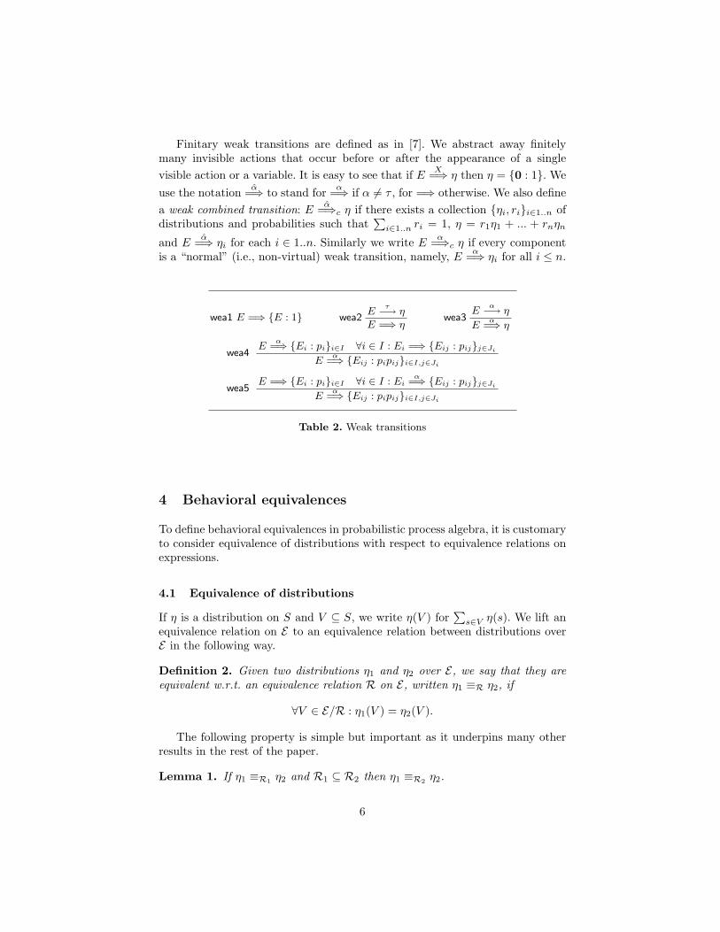
Finitary weak transitions are defined as in [7]. We abstract away finitelymany invisible actions that occur before or after the appearance of a singlevisible action or a variable. It is easy to see that if E

X=⇒ η then η = {0 : 1}. Weuse the notation α=⇒ to stand for α=⇒ if α 6= τ , for =⇒ otherwise. We also definea weak combined transition: E

α=⇒c η if there exists a collection {ηi, ri}i∈1..n ofdistributions and probabilities such that

∑i∈1..n ri = 1, η = r1η1 + ... + rnηn

and Eα=⇒ ηi for each i ∈ 1..n. Similarly we write E

α=⇒c η if every componentis a “normal” (i.e., non-virtual) weak transition, namely, E

α=⇒ ηi for all i ≤ n.

wea1 E =⇒ {E : 1} wea2E

τ−→ η

E =⇒ ηwea3

Eα−→ η

Eα

=⇒ η

wea4E

α=⇒ {Ei : pi}i∈I ∀i ∈ I : Ei =⇒ {Eij : pij}j∈Ji

Eα

=⇒ {Eij : pipij}i∈I,j∈Ji

wea5E =⇒ {Ei : pi}i∈I ∀i ∈ I : Ei

α=⇒ {Eij : pij}j∈Ji

Eα

=⇒ {Eij : pipij}i∈I,j∈Ji

Table 2. Weak transitions

4 Behavioral equivalences

To define behavioral equivalences in probabilistic process algebra, it is customaryto consider equivalence of distributions with respect to equivalence relations onexpressions.

4.1 Equivalence of distributions

If η is a distribution on S and V ⊆ S, we write η(V ) for∑

s∈V η(s). We lift anequivalence relation on E to an equivalence relation between distributions overE in the following way.

Definition 2. Given two distributions η1 and η2 over E, we say that they areequivalent w.r.t. an equivalence relation R on E, written η1 ≡R η2, if

∀V ∈ E/R : η1(V ) = η2(V ).

The following property is simple but important as it underpins many otherresults in the rest of the paper.

Lemma 1. If η1 ≡R1 η2 and R1 ⊆ R2 then η1 ≡R2 η2.

6

Given an equivalence relation R, we construct two relations:

RGdef= {(E | G, F | G) | E R F}

R| def=⋃{RG | G ∈ E}.

Clearly RG and R| are also equivalence relations. If V ∈ E/RGthen we write

V \G for the set {E | E | G ∈ V }. It is easy to see that if V ∈ E/R| then thereexists some expression G such that V ∈ E/RG

. Furthermore, we observe thatV ∈ E/RG

iff V \G ∈ E/R. Suppose θ1 = {Ei : pi}i∈I and θ2 = {Fj : qj}j∈J , weintroduce the following notation:

θ1 | θ2def= {Ei | Fj : piqj}i∈I,j∈J .

The following lemma is crucial for showing the congruence property of strongbisimilarity and observational equivalence (cf. Section 4.4). It says that if twodistributions θ1 and θ2 are equivalent w.r.t. an equivalence relation R, thenthere is a uniform way to extend the two distributions so that the resulting dis-tributions on composed terms are equivalent w.r.t. another equivalence relationR|.

Lemma 2. If θ1 ≡R θ2 then (θ1 | θ) ≡R| (θ2 | θ).

Proof. Let θ = {Gk : pk}k∈K . Without loss of generality, we assume that ifi, j ∈ K and i 6= j then Gi 6= Gj . For any V ∈ E/R| there exists some expressionG such that V ∈ E/RG

. There are two cases:

1. if G 6= Gk for all k ∈ K, then (θ1 | θ)(V ) = 0 = (θ2 | θ)(V );2. if G = Gk for some k ∈ K, then (θ1 | θ)(V ) = rkθ1(V \Gk) = rkθ2(V \Gk) =

(θ2 | θ)(V ).

In summary, (θ1 | θ)(V ) = (θ2 | θ)(V ) for any V ∈ E/R| , i.e., (θ1 | θ) ≡R| (θ2 |θ), which is the required result. ut

Corollary 1. If θ1 ≡R θ2, θ′1 ≡R θ′2 and R is closed under parallel composition,then (θ1 | θ′1) ≡R (θ2 | θ′2).

Proof. If R is closed under parallel composition, then R| ⊆ R. By Lemma 1, wecan state Lemma 2 as: if θ1 ≡R θ2 then (θ1 | θ) ≡R (θ2 | θ). Similarly we canestablish a symmetric property: if θ1 ≡R θ2 then (θ | θ1) ≡R (θ | θ2). As aconsequence we have (θ1 | θ′1) ≡R (θ2 | θ′1) ≡R (θ2 | θ′2). ut

4.2 Behavioral equivalences

Strong bisimulation is defined by requiring equivalence of distributions at everystep. Because of the way equivalence of distributions is defined, we need torestrict to bisimulations which are equivalence relations.

Definition 3. An equivalence relation R ⊆ E × E is a strong bisimulation ifE R F implies:

7

– whenever Eα−→ η1, there exists η2 such that F

α−→ η2 and η1 ≡R η2.

Two expressions E,F are strong bisimilar, written E ∼ F , if there exists astrong bisimulation R s.t. E R F .

We have shown in [16, 15] that to define weak equivalences it is necessary touse weak combined transitions3, so weak probabilistic bisimulation is given inthe following way.

Definition 4. An equivalence relation R ⊆ E ×E is a weak probabilistic bisim-ulation if E R F implies:

– whenever Eα−→ η1, there exists η2 such that F

α=⇒c η2 and η1 ≡R η2.

We write E ≈ F whenever there exists a weak probabilistic bisimulation R s.t.E R F .

As usual, observational equivalence is defined in terms of weak probabilisticbisimulation.

Definition 5. Two expressions E,F are observationally equivalent, written E 'F , if

1. whenever Eα−→ η1, there exists η2 such that F

α=⇒c η2 and η1 ≡≈ η2.2. whenever F

α−→ η2, there exists η1 such that Eα=⇒c η1 and η1 ≡≈ η2.

One can check that all the relations defined above are indeed equivalencerelations and we have the inclusion ordering: ∼ ( ' ( ≈.

Example 1. Consider the following expressions:

E1def= µX(a.X + X)

E2def= µX( 1

2X ⊕ 12 (X + X))

F1def= a.b + τ.c

F2def= F1 + τ.( 1

3F1 ⊕ 23c)

It can be checked that E1 ∼ E2, F1 ≈ F2, and τ.F1 ' τ.F2. Note thatF1 6' F2 because the transition F2

τ−→ {F1 : 13 , c : 2

3} cannot be matched up bythe transition F1

τ−→ {c : 1}, which is the only normal transition from F1 withaction τ . ut

3 The example given in [16, 15] for supporting this argument is built in probabilis-tic automata [29], but it is easy to write a similar example in simple probabilisticautomata (see Appendix A).

8

4.3 Probabilistic “bisimulation up to” techniques

A natural way for showing E ∼ F in a probabilistic process calculus is to con-struct an equivalence relation R which includes the pair (E,F ), and then tocheck that R is a bisimulation. However, it is often difficult to ensure that therelation R one constructs is indeed an equivalence relation. In this case we use“bisimulation up to” techniques. The idea is that we extend R to be R′ suchthat R ⊆ R′ and R′ is easily shown to be a bisimulation.

Given a binary relation R we denote by R∼ the relation (R ∪ ∼)∗, theequivalence closure of R ∪ ∼. Similarly for the notation R≈.

Definition 6. A binary relation R is a strong bisimulation up to ∼ if E R Fimplies:

1. whenever Eα−→ η1, there exists η2 such that F

α−→ η2 and η1 ≡R∼ η2.

2. whenever Fα−→ η2, there exists η1 such that E

α−→ η1 and η1 ≡R∼ η2.

A strong bisimulation up to ∼ is not necessarily an equivalence relation. It isjust an ordinary binary relation included in ∼, as shown by the next proposition.

Proposition 1. If R is a strong bisimulation up to ∼, then R ⊆∼.

For weak probabilistic bisimulation, the “up to” relation can be defined aswell, but we need to be careful.

Definition 7. A binary relation R is a weak probabilistic bisimulation up to ≈if E R F implies:

1. whenever Eα=⇒ η1, there exists η2 such that F

α=⇒c η2 and η1 ≡R≈ η2.

2. whenever Fα=⇒ η2, there exists η1 such that E

α=⇒c η1 and η1 ≡R≈ η2.

In the above definition, we are not able to replace the first double arrow in eachclause by a simple arrow. Otherwise, the resulting relation would not be includedin ≈.

Proposition 2. If R is a weak probabilistic bisimulation up to ≈, then R ⊆≈.

In a way similar to Definition 7, we introduce an “up to '” relation.

Definition 8. A binary relation R is an observational equivalence up to ' ifE R F implies:

1. whenever Eα=⇒ η1, there exists η2 such that F

α=⇒c η2 and η1 ≡R≈ η2.

2. whenever Fα=⇒ η2, there exists η1 such that E

α=⇒c η1 and η1 ≡R≈ η2.

As expected, observational equivalence up to ' is useful because of the fol-lowing property.

Proposition 3. If R is an observational equivalence up to ', then R ⊆'.

9

4.4 Some properties of behavioral equivalences

By using the “bisimulation up to” techniques introduced in the previous section,together with Lemma 2, we can prove the following results. Their detailed proofsare in Appendices B and C, respectively.

Proposition 4 (Properties of ∼).

1. ∼ is a congruence relation;2. µXE ∼ E{µXE/X};3. µX(E + X) ∼ µXE;4. If E ∼ F{E/X} and X is weakly guarded in F , then E ∼ µXF .

Proposition 5 (Properties of ').

1. ' is a congruence relation;2. If τ.E ' τ.E + F and τ.F ' τ.F + E then τ.E ' τ.F ;3. If E ' F{E/X} and X is guarded in F then E ' µXF .

5 Axiomatizing strong bisimilarity

We present in this section the axiom system As for ∼, which includes all ax-ioms and rules displayed in Table 3. We assume the usual rules for equality(reflexivity, symmetry, transitivity and substitutivity), and the alpha-conversionof bound variables. If we omit all the axioms involving probabilities, we obtainthe system composed by S1-3 and R1-3, which characterizes exactly the classof nonprobabilistic finite-state behaviors studied in [25]. The two axioms S4-5allow us to permute and merge probabilistic branches in a probabilistic choice.E is a probabilistic version of the expansion law in CCS.

The notation As ` E = F (and As ` E = F for a finite sequence ofequations) means that the equation E = F is derivable by applying the axiomsand rules from As. The following theorem shows that As is sound with respectto ∼.

Theorem 1 (Soundness of As). If As ` E = E′ then E ∼ E′.

Proof. The soundness of the recursion axioms R1-3 is shown in Section 4.4; thesoundness of S1-4 and E is obvious, and S5 is a consequence of Definition 2. ut

For the completeness proof, the basic points are: (1) if two expressions arebisimilar then we can construct an equation set in a certain format (standardformat) that they both satisfy; (2) if two expressions satisfy the same standardequation set, then they can be proved equal by As. This schema is inspired by[25, 31], but in our case the definition of standard format and the proof itself aremore complicated due to the presence of both probabilistic and nondeterministicdimensions.

10

S1 E + 0 = ES2 E + E = ES3

∑i∈I Ei =

∑i∈I Eρ(i) ρ is any permutation on I

S4 u.⊕

i∈I piEi = u.⊕

i∈I pρ(i)Eρ(i) ρ is any permutation on IS5 u.((

⊕i piEi)⊕ pE ⊕ qE) = u.((

⊕i piEi)⊕ (p + q)E)

R1 µXE = E{µXE/X}R2 If E = F{E/X}, X weakly guarded in F, then E = µXFR3 µX(E + X) = µXE

E Assume E ≡∑

i ui.⊕

j pijEij and F ≡∑

k vk.⊕

l qklFkl. Then infer:

E | F =∑

i ui.⊕

j pij(Eij | F ) +∑

k vk.⊕

l qkl(E | Fkl)

+∑

ui opp vkτ.

⊕j,l(pijqkl)(Eij | Fkl)

where ui opp vk means that ui and vk are complementary actions, i.e., ui = vk.

Table 3. The axiom system As

Definition 9. Let X = {X1, ..., Xm} and W = {W1,W2, ...} be disjoint sets ofvariables. Let H = {H1, ...,Hm} be expressions with free variables in X ∪ W . Inthe equation set S : X = H, we call X formal variables and W free variables.We say S is standard if each Hi takes the form

∑j Ef(i,j) +

∑l Wh(i,l) where

Ef(i,j) = uf(i,j).⊕

k pf(i,j,k)Xg(i,j,k). We call S weakly guarded if there is no Hi

s.t. HiXi−→ {0 : 1}. We say that E provably satisfies S if there are expressions

E = {E1, ..., Em}, with E1 ≡ E and fv(E) ⊆ W , such that As ` E = H{E/X}.

We first recall the theorem of unique solution of equations originally appearedin [25]. Adding probabilistic choice does not affect the validity of this theorem.

Theorem 2 (Unique solution of equations I). If S is a weakly guardedequation set with free variables in W , then there is an expression E which prov-ably satisfies S. Moreover, if F provably satisfies S and has free variables in W ,then As ` E = F .

Proof. Exactly as in [25]. ut

Below we give an extension of Milner’s equational characterization theoremby accommodating probabilistic choice.

Theorem 3 (Equational characterization I). For any expression E, withfree variables in W , there exist some expressions E = {E1, ..., Em}, with E1 ≡ E

and fv(E) ⊆ W , satisfying m equations

As ` Ei =∑

j∈1..n(i)

Ef(i,j) +∑

j∈1..l(i)

Wh(i,j) (i ≤ m)

11

where Ef(i,j) ≡ uf(i,j).⊕

k∈1..o(i,j) pf(i,j,k)Eg(i,j,k).

Proof. By induction on the structure of E. We only consider the case that E ≡F | F ′; all other cases are similar to the proof in [25]. By definition F and F ′ areclosed terms. By induction we have closed terms F1, .., Fm satisfying m equations

As ` Fi =∑

j∈1..n(i)

Ff(i,j) (i ≤ m)

where Ff(i,j) ≡ uf(i,j).⊕

k∈1..o(i,j) pf(i,j,k)Fg(i,j,k). Similarly we have closed ex-pressions F ′

1, ..., F′m′ satisfying m′ equations

As ` F ′i′ =

∑j′∈1..n′(i′)

F ′f ′(i′,j′) (i ≤ m′)

where F ′f ′(i′,j′) ≡ u′f ′(i′,j′).

⊕k′∈1..o′(i′,j′) p′f ′(i′,j′,k′)F

′g′(i′,j′,k′). Now set Ei,i′ ≡

Fi | F ′i′ . By the expansion law E we obtain the equations

As ` Ei,i′ =∑

j∈1..n(i) uf(i,j).⊕

k∈1..o(i,j) pf(i,j,k)Eg(i,j,k),i′

+∑

j′∈1..n′(i′) u′f ′(i′,j′).⊕

k′∈1..o′(i′,j′) p′f ′(i′,j′,k′)Ei,g′(i′,j′,k′)

+∑

uf(i,j) opp u′f′(i′,j′)

τ.⊕

k∈1..o(i,j),k′∈1..o′(i′,j′)(pf(i,j,k)p′f ′(i′,j′,k′))

Ef(i,j,k),f ′(i′,j′,k′)

where i ≤ m, i′ ≤ m′ and uf(i,j) opp u′f ′(i′,j′) means that uf(i,j) and u′f ′(i′,j′)are complementary actions, i.e., they are a and a respectively, for some a, or theinverse.

Moreover, we have E ≡ F1 | F ′1 ≡ E1,1. ut

The following completeness proof is closely analogous to that of [31]. It iscomplicated somewhat by the presence of nondeterministic choice. For example,to construct the formal equations, we need to consider a more refined relationLiji′j′ underneath the relation Kii′ while in [25, 31] it is sufficient to just useKii′ .

Theorem 4 (Completeness of As). If E ∼ E′ then As ` E = E′.

Proof. Let E and E′ have free variables in W . By Theorem 3 there are provableequations such that E ≡ E1, E′ ≡ E′

1 and

As ` Ei =∑

j∈1..n(i)

Ef(i,j) +∑

j∈1..l(i)

Wh(i,j) (i ≤ m)

As ` E′i′ =

∑j′∈1..n′(i′)

E′f ′(i′,j′) +

∑j′∈1..l′(i′)

Wh′(i′,j′) (i′ ≤ m′)

withEf(i,j) ≡ uf(i,j).

⊕k∈1..o(i,j)

pf(i,j,k)Eg(i,j,k)

12

E′f ′(i′,j′) ≡ u′f ′(i′,j′).

⊕k′∈1..o′(i′,j′)

p′f ′(i′,j′,k′)E′g′(i′,j′,k′).

Let I = {〈i, i′〉 | Ei ∼ E′i′}. By hypothesis we have E1 ∼ E′

1, so 〈1, 1〉 ∈ I.Moreover, for each 〈i, i′〉 ∈ I, the following holds, by the definition of strongbisimilarity:

1. There exists a total surjective relation Kii′ between {1, ..., n(i)} and {1, ..., n′(i′)},given by

Kii′ = {〈j, j′〉 | 〈f(i, j), f ′(i′, j′)〉 ∈ I}.

Furthermore, for each 〈j, j′〉 ∈ Kii′ , we have uf(i,j) = u′f ′(i′,j′) and there ex-ists a total surjective relation Liji′j′ between {1, ..., o(i, j)} and {1, ..., o′(i′, j′)},given by

Liji′j′ = {〈k, k′〉 | 〈g(i, j, k), g′(i′, j′, k′)〉 ∈ I}.2. As `

∑j∈1..l(i) Wh(i,j) =

∑j′∈1..l′(i′) Wh′(i′,j′).

Now, let Liji′j′(k) denote the image of k ∈ {1, ..., o(i, j)} under Liji′j′ andL−1

iji′j′(k′) the preimage of k′ ∈ {1, ..., o′(i′, j′)} under Liji′j′ . We write [k]iji′j′

for the set L−1iji′j′(Liji′j′(k)) and [k′]iji′j′ for Liji′j′(L−1

iji′j′(k′)). It follows from

the definitions that

1. If 〈i, i′1〉 ∈ I, 〈i, i′2〉 ∈ I, 〈j, j′1〉 ∈ Kii′1and 〈j, j′2〉 ∈ Kii′2

, then [k]iji′1j′1=

[k]iji′2j′2.

2. If q1 ∈ [k]iji′j′ and q2 ∈ [k]iji′j′ , then Eg(i,j,q1) ∼ Eg(i,j,q2).

Define νijk =∑

q∈[k]iji′j′pf(i,j,q) for any i′, j′ such that 〈i, i′〉 ∈ I and 〈j, j′〉 ∈

Kii′ ; define ν′i′j′k′ =∑

q′∈[k′]iji′j′p′f ′(i′,j′,q′) for any i, j such that 〈i, i′〉 ∈ I and

〈j, j′〉 ∈ Kii′ . It is easy to see that whenever 〈i, i′〉 ∈ I, 〈j, j′〉 ∈ Kii′ and〈k, k′〉 ∈ Liji′j′ then νijk = ν′i′j′k′ .

We now consider the formal equations, one for each 〈i, i′〉 ∈ I:

Xi,i′ =∑

〈j,j′〉∈Kii′

Hf(i,j),f ′(i′,j′) +∑

j∈1..l(i)

Wh(i,j)

where

Hf(i,j),f ′(i′,j′) ≡ uf(i,j).⊕

〈k,k′〉∈Liji′j′

(pf(i,j,k)p

′f ′(i′,j′,k′)

νijk)Xg(i,j,k),g′(i′,j′,k′).

These equations are provably satisfied when each Xi,i′ is instantiated to Ei, sinceKii′ and Liji′j′ are total and the right-hand side differs at most by repeatedsummands from that of the already proved equation for Ei. Note that eachprobabilistic branch pf(i,j,k)Eg(i,j,k) in the subterm Ef(i,j) of Ei becomes theprobabilistic summation of several branches like⊕

q′∈[k′]iji′j′

(pf(i,j,k)p

′f ′(i′,j′,q′)

νijk)Eg(i,j,k)

13

in Hf(i,j),f ′(i′,j′){Ei/Xi,i′}i, where 〈i, i′〉 ∈ I, 〈j, j′〉 ∈ Kii′ and 〈k, k′〉 ∈ Liji′j′ .But they are provably equal because∑

q′∈[k′]iji′j′(

pf(i,j,k)p′f′(i′,j′,q′)

νijk) = pf(i,j,k)

νijk·∑

q′∈[k′]iji′j′p′f ′(i′,j′,q′)

= pf(i,j,k)

νijk· ν′i′j′k′ = pf(i,j,k)

and then the axiom S5 can be used. Symmetrically, the equations are provablysatisfied when each Xi,i′ is instantiated to E′

i′ ; this depends on the surjectivityof Kii′ and Jiji′j′ .

Finally, we note that each Xi,i′ is weakly guarded in the right-hand sidesof the formal equations. It follows from Theorem 2 that ` Ei = E′

i′ for each〈i, i′〉 ∈ I, and hence ` E = E′. ut

6 Axiomatizing observational equivalence

In this section we axiomatize the observational equivalence '. We are not able togive a complete axiomatization for the whole set of expressions (and we conjec-ture that it is not possible), so we restrict to the subset of E consisting of guardedexpressions only. An expression is guarded if for each of its subexpression of theform µXF , the variable X is guarded in F (cf. Definition 1).

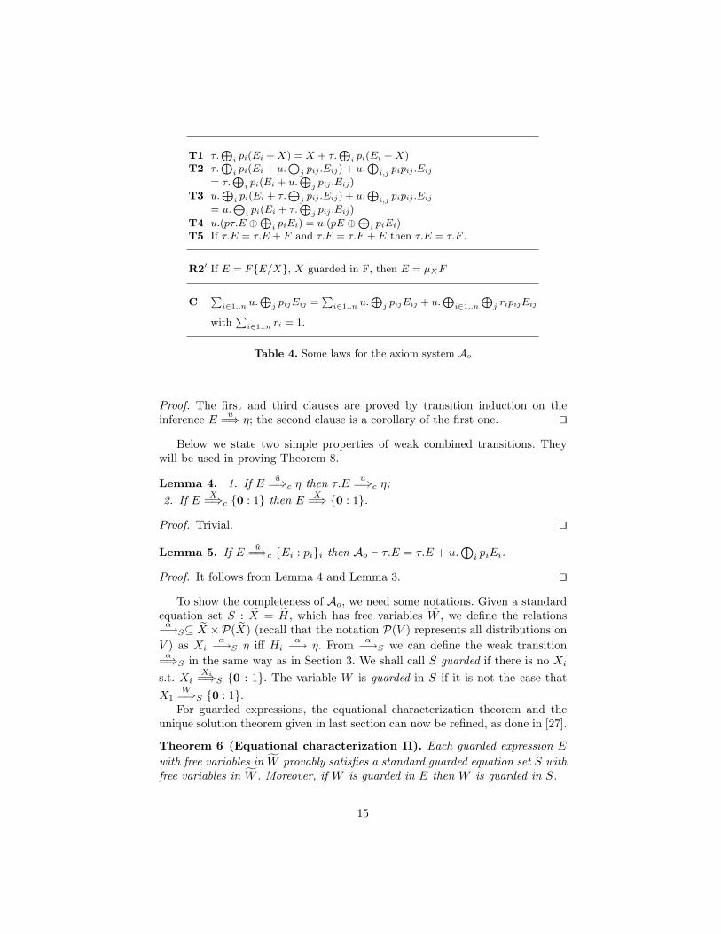
First let us analyze the system As. All axioms except for R2-3 are still validfor '. R3 is not needed because it deals with unguarded expressions. We canreuse R2 by requiring X to be (strongly) guarded, so we get R2′ in Table 4. Toestablish the system Ao for ', we use five τ -laws, T1-5 in Table 4, to abstractaway invisible actions. Note that T1 and T2 together constitute the probabilisticversion of Milner’s second τ -law ([27] page 231). T3 and T4 are the probabilisticextensions of Milner’s third and first τ -laws, respectively. The extra rule T5 hasno nonprobabilistic counterpart in CCS, but it plays an important role in theproof of Theorem 8. As in [7] the axiom C is needed because we use combinedtransitions when defining observational equivalence.

Theorem 5 (Soundness of Ao). If Ao ` E = F then E ' F .

Proof. The rules R2′ and T5 are proved to be sound in Proposition 5 (its proofis detailed in Appendix C). The soundness of C and T1-4 is straightforward. ut

For the completeness proof, it is convenient to use the following saturationproperty, which relates operational semantics to term transformation, and whichcan be shown by using the probabilistic τ -laws T1-4 and the axiom C.

Lemma 3 (Saturation). Suppose there is no parallel composition in E.

1. If Eu=⇒ η with η = {Ei : pi}i, then Ao ` E = E + u.

⊕i piEi;

2. If Eu=⇒c η with η = {Ei : pi}i, then Ao ` E = E + u.

⊕i piEi;

3. If EX=⇒ {0 : 1} then Ao ` E = E + X.

14

T1 τ.⊕

i pi(Ei + X) = X + τ.⊕

i pi(Ei + X)T2 τ.

⊕i pi(Ei + u.

⊕j pij .Eij) + u.

⊕i,j pipij .Eij

= τ.⊕

i pi(Ei + u.⊕

j pij .Eij)

T3 u.⊕

i pi(Ei + τ.⊕

j pij .Eij) + u.⊕

i,j pipij .Eij

= u.⊕

i pi(Ei + τ.⊕

j pij .Eij)

T4 u.(pτ.E ⊕⊕

i piEi) = u.(pE ⊕⊕

i piEi)T5 If τ.E = τ.E + F and τ.F = τ.F + E then τ.E = τ.F .

R2′ If E = F{E/X}, X guarded in F, then E = µXF

C∑

i∈1..n u.⊕

j pijEij =∑

i∈1..n u.⊕

j pijEij + u.⊕

i∈1..n

⊕j ripijEij

with∑

i∈1..n ri = 1.

Table 4. Some laws for the axiom system Ao

Proof. The first and third clauses are proved by transition induction on theinference E

u=⇒ η; the second clause is a corollary of the first one. ut

Below we state two simple properties of weak combined transitions. Theywill be used in proving Theorem 8.

Lemma 4. 1. If Eu=⇒c η then τ.E

u=⇒c η;2. If E

X=⇒c {0 : 1} then EX=⇒ {0 : 1}.

Proof. Trivial. ut

Lemma 5. If Eu=⇒c {Ei : pi}i then Ao ` τ.E = τ.E + u.

⊕i piEi.

Proof. It follows from Lemma 4 and Lemma 3. ut

To show the completeness of Ao, we need some notations. Given a standardequation set S : X = H, which has free variables W , we define the relations

α−→S⊆ X ×P(X) (recall that the notation P(V ) represents all distributions onV ) as Xi

α−→S η iff Hiα−→ η. From α−→S we can define the weak transition

α=⇒S in the same way as in Section 3. We shall call S guarded if there is no Xi

s.t. XiXi=⇒S {0 : 1}. The variable W is guarded in S if it is not the case that

X1W=⇒S {0 : 1}.

For guarded expressions, the equational characterization theorem and theunique solution theorem given in last section can now be refined, as done in [27].

Theorem 6 (Equational characterization II). Each guarded expression E

with free variables in W provably satisfies a standard guarded equation set S withfree variables in W . Moreover, if W is guarded in E then W is guarded in S.

15

Proof. By induction on the structure of E. Consider the case that E ≡ u.⊕

i∈I piEi.For each i ∈ I, let Xi be the distinguished variable of the equation set Si for Ei.We can define S as {X = u.

⊕i∈I piXi} ∪

⋃i∈I Si, with the new variable X dis-

tinguished. All other cases are the same as in [27]. For the case that E ≡ F | F ′,the arguments are similar to those in Theorem 3. ut

Theorem 7 (Unique solution of equations II). If S is a guarded equationset with free variables in W , then there is an expression E which provably satisfiesS. Moreover, if F provably satisfies S and has free variables in W , then Ao `E = F .

Proof. Nearly the same as the proof of Theorem 2, just replacing the recursionrule R2 with R2′. ut

The following theorem plays a crucial role in proving the completeness of Ao.

Theorem 8. Let E provably satisfy S and F provably satisfy T , where both Sand T are standard, guarded equation sets, and let E ' F . Then there is astandard, guarded equation set U satisfied by both E and F .

Proof. Suppose that X = {X1, ..., Xm}, Y = {Y1, ..., Yn} and W = {W1,W2, ...}are disjoint sets of variables. Let

S : X = H

T : Y = J

with fv(H) ⊆ X ∪ W , fv(J) ⊆ Y ∪ W , and that there are expressions E ={E1, ..., Em} and F = {F1, ..., Fn} with E1 ≡ E, F1 ≡ F , and fv(E)∪fv(F ) ⊆ W ,so that

Ao ` E = H{E/X}

Ao ` F = J{F /Y }.

Consider the least equivalence relation R ⊆ (X ∪ Y )× (X ∪ Y ) such that

1. whenever (Z,Z ′) ∈ R and Zα−→ η, then there exists η′ s.t. Z ′ α=⇒c η′ and

η ≡R η′;2. (X1, Y1) ∈ R and if X1

α−→ η then there exists η′ s.t. Y1α=⇒c η′ and η ≡R η′.

Clearly R is a weak probabilistic bisimulation on the transition system overX∪ Y , determined by →def=→S ∪ →T . Now for two given distributions η = {Xi :pi}i∈I , η′ = {Yj : qj}j∈J , with η ≡R η′, we introduce the following notations:

Kη,η′ = {(i, j) | i ∈ I, j ∈ J, and (Xi, Yj) ∈ R}νi =

∑{pi′ | i′ ∈ I, and (Xi, Xi′) ∈ R} for i ∈ I

νj =∑{pj′ | j′ ∈ J, and (Yj , Yj′) ∈ R} for j ∈ J

16

Since η ≡R η′ it follows by definition that if (i, j) ∈ Kη,η′ , for some η, η′, thenνi = νj . Thus we can define the expression

Gη,η′def=

⊕(i,j)∈Kη,η′

piqj

νiZij

which will play the same role as the expression Hf(i,j),f ′(i′,j′) in the proof ofTheorem 4.

Based on the above R we choose a new set of variables Z such that

Z = {Zij | Xi ∈ X, Yj ∈ Y and (Xi, Yj) ∈ R}.

Furthermore, for each Zij ∈ Z we construct three auxiliary finite sets of expres-sions, denoted by Aij , Bij and Cij , by the following procedure.

1. Initially the three sets are empty.2. For each η with Xi

α−→ η, arbitrarily choose one (and only one — the sameprinciple applies in other cases too) η′ (if it exists) satisfying η ≡R η′ andYj

α=⇒c η′. If α ∈ Act then we construct the expression Gη,η′ and updateAij to be Aij ∪ {α.Gη,η′}; if α = X for some X then we update Aij to beAij ∪ {X}. Similarly for each η′ with Yj

α−→ η′, arbitrarily choose one η (ifit exists) satisfying η ≡R η′ and Xi

α=⇒c η. If α ∈ Act then we construct theexpression Gη,η′ and update Aij to be Aij ∪{α.Gη,η′}; if α = X for some Xthen we update Aij to be Aij ∪ {X}.

3. For each η with Xiτ−→ η, arbitrarily choose one η′ (if it exists) satisfying

η ≡R η′, Yj =⇒c η′ but not Yjτ=⇒c η′, construct the expression Gη,η′ and

update Bij to be Bij ∪ {τ.Gη,η′}.4. For each η′ with Yj

τ−→ η′, arbitrarily choose one η (if it exists) satisfyingη ≡R η′, Xi =⇒c η but not Xi

τ=⇒c η, construct Gη,η′ and update Cij to beCij ∪ {τ.Gη,η′}.

Clearly the three sets constructed in this way are finite. Now we build a newequation set

U : Z = L

where U11 is the distinguished variable and

Lij =

{∑G∈Aij

G if Bij ∪ Cij = ∅τ.(

∑G∈Aij∪Bij∪Cij

G) otherwise.

We assert that E provably satisfies the equation set U . To see this, we chooseexpressions

Gij ={

Ei if Bij ∪ Cij = ∅τ.Ei otherwise

and verify that Ao ` Gij = Lij{G/Z}.

17

In the case that Bij ∪ Cij = ∅, all those summands of Lij{G/Z} which arenot variables are of the form:

u.⊕

(i,j)∈Kη,η′

piqj

νiE′

i

where E′i = Ei or E′

i = τ.Ei for each i. By T4 we can prove that

u.⊕

(i,j)∈Kη,η′

piqj

νiE′

i = u.⊕

(i,j)∈Kη,η′

piqj

νiEi.

Then by some arguments similar to those in Theorem 4, together with Lemma 3,we can show that

Ao ` Lij{G/Z} = Hi{E/X} = Ei.

On the other hand, if Bij ∪ Cij 6= ∅, we let Cij = {D1, ..., Do} (Cij = ∅ is aspecial case of the following argument) and D =

∑l∈1..o Dl{G/Z}. As in last

case we can show that

Ao ` Lij{G/Z} = τ.(Hi{E/X}+ D).

For any l with 1 ≤ l ≤ o, let Dl{G/Z} = τ.⊕

k pkEk. It is easy to see thatEi =⇒c η with η = {Ek : pk}k. So by Lemma 5 it holds that

Ao ` τ.Ei = τ.Ei + Dl{G/Z}.

As a result we can infer

Ao ` τ.Ei = τ.Ei + D = τ.Ei + (Ei + D).

by Lemma 3. Similarly,

Ao ` τ.(Ei + D) = τ.(Ei + D) + Ei.

Consequently it follows from T5 that

Ao ` τ.Ei = τ.(Ei + D) = τ.(Hi{E/X}+ D) = Lij{G/Z}.

In the same way we can show that F provably satisfies U . At last U is guardedbecause S and T are guarded. utTheorem 9 (Completeness of Ao). If E and F are guarded expressions andE ' F , then Ao ` E = F .

Proof. A direct consequence by combining Theorems 6, 8 and 7. utIn the axiom system Ao the rule T5 deserves more explanations. For the two

expressions F1, F2 given in Example 1 (cf. Section 4.2), we can derive the equalityτ.F1 = τ.F2 by using T5. Alternatively, we could use the following axiom

τ.E = τ.(E + τ.((1− p)E ⊕⊕

i ppiEi)) where E = τ.(τ.⊕

i piEi + F )

which is sound and indeed derivable from T5. In fact, we could have introducedthe cumbersome axiom in place of T5 in the axiomatization for ' — we wouldstill be able to prove Theorem 8 and the completeness of the alternative axiom-atization. In this paper we have chosen T5 instead merely because it looks moreelegant than the above axiom.

18

7 Conclusion and related work

We have proposed a probabilistic process calculus which combines both nonde-terministic and probabilistic behavior in the style of Segala and Lynch’s simpleprobabilistic automata. The calculus also admits a restricted form of parallelcomposition to allow for compositional reasoning of finite-state behaviors. Wehave presented sound and complete axiomatizations for two behavioral equiva-lences: strong bisimilarity and observational equivalence.

In CCS there are other static operators such as restriction and relabeling thatare not studied in this paper. As parallel composition, these operators shouldbe dealt with carefully. For example, the expression µX((a.X | a)\a) appears tobe guarded (cf. Definition 1), but actually it is strongly bisimilar to µX(τ.X)thus should be deemed unguarded. When considering axiomtizations one tendsto disallow this kind of expressions by imposing the constraint that free variablesdo not occur in the scope of static operators [11, 5].

As we said before, in this paper many concepts and proof techniques are in-herited from [16, 15]. The main differences are as follows: (i) in this paper we haveadded a parallel composition operator to our probabilistic process calculus; (ii)to define the operational semantics of this operator we restrict ourself to simpleprobabilistic automata, while the results of [16, 15] are valid for all probabilisticautomata; (iii) besides strong bisimilarity and observational equivalence, in [16,15] we also axiomatized two other equivalences: a strong probabilistic bisimilar-ity and a divergency-sensitive equivalence. We think that it should be possibleto adapt those results to the framework of this paper.

In [25] and [27] Milner gave complete axiomatizations for strong bisimilarityand observational equivalence, respectively, for a core CCS [26]. Our results inSection 5 and Section 6 extend [25] and [27] (for guarded expressions) respec-tively, to a strictly larger language with a probabilistic choice and a parallelcomposition operator.

Bandini and Segala [7] axiomatized two strong and two weak equivalences fora language similar to the fragment of our calculus without recursion and paral-lelism. They considered two types of semantics. In both cases, their completenessproofs are done by structural induction on processes, which is, of course, impos-sible in our setting because of recursion.

Giacalone, Jou and Smolka [18] axiomatized strong bisimulation for a fullyprobabilistic (i.e. without nondeterminism) extension of Milner’s SCCS [24],where parallel composition is synchronous. In contrast, we consider an asyn-chronous parallel composition and we admit nondeterminism.

Baeten, Bergstra and Smolka [4] proposed a probabilistic ACP by introduc-ing a parameterized composition. They considered generative models, which arefully probabilistic, and axiomatized strong probabilistic bisimilarity for finiteprocesses (without recursion).

Andova [3] studied a different version of probabilistic ACP by allowing nonde-terminism and a parallel composition which is not parameterized. She provideda sound and complete axiomatization for strong probabilistic bisimilarity in the

19

case of finite processes. She also gave some sound verification rules for proba-bilistic branching bisimilarity in a fully probabilistic model without parallelism.

Strong probabilistic bisimilarity was also axiomatized by Stark and Smolkain [31]. They gave a probabilistic version of the results of [25]. However, nei-ther nondeterminism nor parallelism is considered. Later the same calculus wasstudied in [1], which uses some axioms from iteration algebra to characterizerecursion.

In the nonprobabilistic setting, Bergstra and Klop [10] established a soundand complete axiomatization for regular processes with τ -steps and free merge(which allows arbitrary interleaving but no communication). They required thatfree merge should not appear in the body of any recursive expression. To give alinearization algorithm for pCRL, Groote, Ponse and Usenko adopted a similarrestriction for parallel composition [19]. Usenko extended this result to µCRL inhis thesis [33]. In this paper our parallel composition operator allows communi-cation and it can appear in the body of a recursive expression, though only in arestricted way. For example, the expression

µX(a.X + a.µY (b.Y ) | a.µZ(c.Z))

is a legal expression in our calculus and we are able to manipulate it in our axiomsystems.

Baeten and Bravetti [5] axiomatized observational equivalence in a genericprocess algebra. Their restriction enforced to parallel composition is the same asours in spirit. Interestingly, they reduced two of Milner’s axioms for unguardedrecursion [27] to just a single axiom. It remains open whether their results canbe adapted to a probabilistic setting. Similarly, it might be interesting to extendvan Glabbeek’s axiomatization for branching congruence [34] to a probabilisticsetting. We believe that the general proof schema laid out in this paper could bereused for branching congruence, but the soundness proof of some axioms suchas R2′ would be very complicated because, besides the probabilistic and non-deterministic features, we need to consider the branching structure of processes,which is ignored in observational congruence.

Christensen, Hirshfeld and Moller studied a class of standard form CCS [13]where open expressions are allowed to be put in parallel composition. In that lan-guage, strong bisimulation is decidable and they obtained a sound and completesequent based equational theory, but observational equivalence is semi-decidable[12]. In this paper we follow [25, 27] and characterize recursion by laws concern-ing the explicit fixed point operator µ, while we capture by τ -laws the differencebetween observational equivalence and strong bisimulation.

Several works in the literature address the problem of how to define appro-priate parallel composition operators on various probabilistic models, see [14]for more discussions and [30] for a good survey. In this paper, we work at simpleprobabilistic automata where parallel composition is easy to define (cf. Table 1).

20

References

1. L. Aceto, Z. Esik, and A. Ingolfsdottir. Equational axioms for probabilistic bisim-ilarity (preliminary report). Technical Report RS-02-6, BRICS, 2002.

2. L. Aceto and W. J. Fokkink. The quest for equational axiomatizations of parallelcomposition: Status and open problems. In Proceedings of the Workshop on Al-gebraic Process Calculi: The First Twenty Five Years and Beyond, BRICS NotesSeries, 2005. To appear.

3. S. Andova. Probabilistic Process Algebra. PhD thesis, Eindhoven University ofTechnology, 2002.

4. J. C. M. Baeten, J. A. Bergstra, and S. A. Smolka. Axiomatizing probabilis-tic processes: ACP with generative probabilities. Information and Computation,121(2):234–255, 1995.

5. J. C. M. Baeten and M. Bravetti. A ground-complete axiomatization of finite stateprocesses in process algebra. In Proceedings of the 16th International Conferenceon Concurrency Theory, Lecture Notes in Computer Science. Springer, 2005. Toappear.

6. J. C. M. Baeten and W. P. Weijland. Process Algebra, volume 18 of CambridgeTracts in Theoretical Computer Science. Cambridge University Press, 1990.

7. E. Bandini and R. Segala. Axiomatizations for probabilistic bisimulation. InProceedings of the 28th International Colloquium on Automata, Languages andProgramming, volume 2076 of Lecture Notes in Computer Science, pages 370–381.Springer, 2001.

8. J. A. Bergstra and J. W. Klop. Process algebra for synchronous communications.Information and Control, 60:109–137, 1984.

9. J. A. Bergstra and J. W. Klop. Verification of an alternating bit protocol bymeans of process algebra. In Proceedings of the International Spring School onMathematical Methods of Specification and Synthesis of Software Systems, volume215 of Lecture Notes in Computer Science, pages 9–23. Springer, 1986.

10. J. A. Bergstra and J. W. Klop. A complete inference system for regular processeswith silent moves. In Proceedings of Logic Colloquium 1986, pages 21–81. NorthHolland, Amsterdam, 1988.

11. M. Bravetti and R. Gorrieri. Deciding and axiomatizing weak ST bisimulationfor a process algebra with recursion and action refinement. ACM Transactions onComputational Logic, 3(4):465–520, 2002.

12. S. Christensen. Decidability and Decomposition in Process Algebras. PhD thesis,University of Edinburgh, 1993.

13. S. Christensen, Y. Hirshfeld, and F. Moller. Decidable subsets of ccs. ComputerJournal, 37(4):233–242, 1994.

14. P. R. D’Argenio, H. Hermanns, and J.-P. Katoen. On generative parallel compo-sition. Electronic Notes in Theoretical Computer Science, 22, 1999.

15. Y. Deng. Axiomatisations and types for probabilistic and mobile processes. PhDthesis, Ecole des Mines de Paris, 2005.

16. Y. Deng and C. Palamidessi. Axiomatizations for probabilistic finite-state behav-iors. In Proceedings of the 8th International Conference on Foundations of SoftwareScience and Computation Structures, volume 3441 of Lecture Notes in ComputerScience, pages 110–124. Springer, 2005.

17. W. J. Fokkink, J. F. Groote, J. Pang, B. Badban, and J. C. van de Pol. Verifyinga sliding window protocol in µCRL. In 10th Conference on Algebraic Methodologyand Software Technology, Proceedings, volume 3116 of Lecture Notes in ComputerScience, pages 148–163. Springer, 2004.

21

18. A. Giacalone, C.-C. Jou, and S. A. Smolka. Algebraic reasoning for probabilisticconcurrent systems. In Proceedings of IFIP WG 2.2/2.3 Working Conference onProgramming Concepts and Methods, pages 453–459, 1990.

19. J. F. Groote, A. Ponse, and Y. S. Usenko. Linearization in parallel pCRL. Journalof Logic and Algebraic Programming, 48(1-2):39–72, 2001.

20. M. Hennessy and R. Milner. Algebraic laws for nondeterminism and concurrency.Journal of ACM, 32:137–161, 1985.

21. C. A. R. Hoare. Communicating Sequential Processes. Prentice Hall, 1985.22. K. G. Larsen and A. Skou. Bisimulation through probabilistic testing. Information

and Computation, 94(1):1–28, 1991.23. N. A. Lynch, I. Saias, and R. Segala. Proving time bounds for randomized dis-

tributed algorithms. In Proceedings of the 13th Annual ACM Symposium on thePrinciples of Distributed Computing, pages 314–323, 1994.

24. R. Milner. Calculi for synchrony and asynchrony. Theoretical Computer Science,25:267–310, 1983.

25. R. Milner. A complete inference system for a class of regular behaviours. Journalof Computer and System Science, 28:439–466, 1984.

26. R. Milner. Communication and Concurrency. Prentice-Hall, 1989.27. R. Milner. A complete axiomatisation for observational congruence of finite-state

behaviours. Information and Computation, 81:227–247, 1989.28. A. Pogosyants, R. Segala, and N. A. Lynch. Verification of the randomized con-

sensus algorithm of Aspnes and Herlihy: a case study. Distributed Computing,13(3):155–186, 2000.

29. R. Segala and N. A. Lynch. Probabilistic simulations for probabilistic processes. InProceedings of the 5th International Conference on Concurrency Theory, volume836 of Lecture Notes in Computer Science, pages 481–496. Springer, 1994.

30. A. Sokolova and E. P. de Vink. Probabilistic automata: system types, parallelcomposition and comparison. In Validation of Stochastic Systems: A Guide toCurrent Research, volume 2925 of Lecture Notes in Computer Science, pages 1–43.Springer, 2004.

31. E. W. Stark and S. A. Smolka. A complete axiom system for finite-state proba-bilistic processes. In Proof, language, and interaction: essays in honour of RobinMilner, pages 571–595. MIT Press, 2000.

32. M. Stoelinga and F. Vaandrager. Root contention in IEEE 1394. In Proceedingsof the 5th International AMAST Workshop on Formal Methods for Real-Time andProbabilistic Systems, volume 1601 of Lecture Notes in Computer Science, pages53–74. Springer, 1999.

33. Y. S. Usenko. Linearization in µCRL. PhD thesis, Edindhoven University ofTechnology, 2002.

34. R. J. van Glabbeek. A complete axiomatization for branching bisimulation congru-ence of finite-state behaviours. In Proceedings of the 18th International Symposiumon Mathematical Foundations of Computer Science, volume 711 of Lecture Notesin Computer Science, pages 473–484. Springer, 1993.

22

Appendix

A Transitivity of Weak Bisimulation

It seems natural to define weak bisimulation in the following way.

Definition (Tentative). An equivalence relation R ⊆ E × E is a weak bisimu-lation if E R F implies:

– whenever Eα−→ η1, there exists η2 such that F

α=⇒ η2 and η1 ≡R η2.

E and F are weak bisimilar, written E � F , whenever there exists a weakbisimulation R s.t. E R F .

Unfortunately the above definition is incorrect because it defines a relationwhich is not transitive. To see this, consider the following expressions:

Rdef= τ.( 1

2a⊕ 12b)

Edef= τ.( 1

2R⊕ 12R) + τ.( 1

2R⊕ 14a⊕ 1

4b)F

def= τ.( 12R⊕ 1

2R)G

def= τ.R

It can be checked that E � F and F � G but E 6� G. The transition Eτ−→ η

cannot be matched by any of the three possible weak transitions from G : G =⇒ηi (i = 1, 2, 3), where η1 = {G : 1}, η2 = {R : 1} and η3 = {a : 1

2 , b : 12}, since

neither η1 nor η2 nor η3 is equivalent to η.To obtain a transitive weak bisimilarity, we have used combined weak tran-

sitions in Definition 4.

B Proof of Proposition 4

Lemma 6. If fv(E) ⊆ {X, Z} and Z 6∈ fv(F ), then

E{E′/Z}{F /X} ≡ E{F /X}{E′{F /X}/Z}.

Proof. By induction on the structure of E. ut

Lemma 7. Let η = r1η1+...+rnηn and η′ = r1η′1+...+rnη′n with

∑i∈1..n ri = 1.

If ηi ≡R η′i for each i ≤ n, then η ≡R η′.

Proof. For any V ∈ E/R, we have

η(V ) =∑

i∈1..n

riηi(V ) =∑

i∈1..n

riη′i(V ) = η′(V ).

Therefore η ≡R η′ by definition. ut

23

Proposition 6. If E ∼ F then E | G ∼ F | G.

Proof. We show that the relation ∼| is a strong bisimulation. There are fourcases, among which we consider two of them, the others are similar.

Case 1: Suppose η1 = {Ei | G : pi}i and E | Gα−→ η1 is derived from

the transition Eα−→ θ1 = {Ei : pi}i. Since E ∼ F , there exists θ2 such that

Fα−→ θ2 and θ1 ≡∼ θ2. Let θ2 = {Fj : qj}j , by rule par we have the transition

F | Gα−→ {Fj | G : qj}j = η2. Let θ = {G : 1}, then we have η1 = θ1 | θ and

η2 = θ2 | θ. By Lemma 2 it follows that η1 ≡∼| η2.Case 2: Suppose E

a−→ θ1, Ga−→ θ, and E | G

τ−→ η1 with η1 = θ1 | θ.Since E ∼ F , there exists θ2 such that F

a−→ θ2 and θ1 ≡∼ θ2. By rule com wehave the transition F | G

τ−→ η2 with η2 = θ2 | θ. By Lemma 2 it follows thatη1 ≡∼| η2. ut

Proposition 7. If E ∼ F then E{G/X} ∼ F{G/X} for any G ∈ E.

Proof. Similar to the proof of Proposition 13, which is detailed in next section.ut

Proposition 8. If E ∼ F then µXE ∼ µXF .

Proof. Let ρdef= {µXE/X} and σ

def= {µXF/X}. We show that the relation

R = {(Gρ, Gσ) | fv(G) ⊆ {X}}

is a strong bisimulation up to ∼. Because of symmetry we only show the asser-tion:

“if Gρα−→ η1 then there exists η2 s.t. Gσ

α−→ η2 and η1 ≡R∼ η2”by induction on the depth of the inference Gσ → η1. There are several cases,depending on the structure of G.

1. G ≡ X: Then Gρ ≡ µXEα−→ η1 and there is a shorter inference Eρ

α−→ η1.By induction hypothesis there is some θ s.t. Eσ

α−→ θ and η1 ≡R∼ θ. SinceE ∼ F we know that Eσ ∼ Fσ by Proposition 7. Hence there exists someη2 s.t. Fσ

α−→ η2 and θ ≡∼ η2. By Lemma 1 and the transitivity of ≡R∼ itfollows that η1 ≡R∼ η2.

2. G ≡ u.⊕

i piGi: Then we have Gρu−→ η1 ≡ {Giρ : pi}i and Gσ

u−→ η2 ≡{Giσ : pi}i. Since Giρ R Giσ, it is easy to see that η1 ≡R∼ η2.

3. G ≡∑

i∈1..m Gi: If Gρα−→ η1, then Gjρ

α−→ η1 for some j ∈ 1..m, by ashorter inference. By induction hypothesis we have that Gjσ

α−→ η2 suchthat η1 ≡R∼ η2.

4. G ≡ µY G′: If Gρα−→ η1 then G′ρ{Gρ/Y } by a shorter inference. Since

G′ρ{Gρ/Y } ≡ (G′{G/Y })ρ we have that (G′{G/Y })ρ α−→ η1. By induc-tion hypothesis it follows that (G′{G/Y })σ α−→ η2 with η1 ≡R∼ η2. ThusG′σ{Gσ/Y } α−→ η2, which implies Gσ

α−→ η2 by the rule rec.

24

5. G ≡ G1 | G2: Suppose Gρα−→ η1. Depending on the last rule used for

deriving the transition, there are four cases. We consider one typical casewhere the last rule used is com. So we have the transitions G1ρ

a−→ θ1,G2ρ

a−→ θ′1 and Gρτ−→ η1 with η1 = θ1 | θ′1. By induction hypothesis

we have the simulating transitions G1σa−→ θ2 and G2σ

a−→ θ′2 such thatθ1 ≡R∼ θ2 and θ′1 ≡R∼ θ′2. By rule com we infer that Gσ

τ−→ η2 withη2 = θ2 | θ′2. It is easy to see thatR is closed under parallel composition (herewe need the condition of composing closed expressions). By Proposition 6we know that ∼ is also closed under parallel composition. It follows that R∼is closed under parallel composition as well. Therefore by Corollary 1 we canderive that η1 ≡R∼ η2.

ut

Proposition 9 (Congruence). If E ∼ F then

1. u.⊕

i piEi ∼ u.⊕

i piFi;2.

∑i Ei ∼

∑i Fi;

3. E1 | E2 ∼ F1 | F2;4. µXE1 ∼ µXF1.

Proof. The first two clauses are easy to prove; the last two follow from Proposi-tion 6 and Proposition 8 respectively. ut

Proposition 10. µXE ∼ E{µXE/X}.

Proof. Observe that µXEα−→ η iff E{µXE/X} α−→ η. ut

Proposition 11. µX(E + X) ∼ µXE

Proof. Let ρdef= {µX(E+X)/X} and σ

def= {µXE/X}. We show that the relation

R = {(Gρ, Gσ | fv(G ⊆ {X}))}

is a strong bisimulation up to ∼. We prove the following two assertions:

1. If Gρα−→ η1 then Gσ

α−→ η2 and η1 ≡R∼ η2;2. If Gσ

α−→ η2 then Gρα−→ η1 and η1 ≡R∼ η2.

The proof is carried out by induction on transitions, similar to the proof ofProposition 8. Here we only consider the case that G ≡ X.

1. If Gρ ≡ Xρα−→ η1 then (E+X)ρ α−→ η1 by a shorter inference. By induction

hypothesis it follows that (E + X)σ α−→ η2 and η1 ≡R∼ η2. Then eitherEσ

α−→ η2 or Xσα−→ η2. From the first case we can also obtain Xσ

α−→ η2

by rule rec. Therefore in both cases we have Gσα−→ η2.

2. If Gσ ≡ Xσα−→ η2 then Eσ

α−→ η2 by a shorter inference. By inductionhypothesis it follows that Eρ

α−→ η1 with η1 ≡R∼ η2. By the rule nsum wederive (E +X)ρ α−→ η1. By rec we get the required result that Gρ ≡ Xρ

α−→η1.

25

ut

Lemma 8. Suppose fv(G) ⊆ {X} and all free occurrences of X in G are weaklyguarded. If G{E/X} α−→ η1 with η1 ≡ {Gi : pi}i then Gi takes the formG′

i{E/X}; Moreover, for any F , G{F/X} α−→ η2 with η2 ≡ {G′i{F/X} : pi}i

and η1 ≡R∼ η2 where

R = {(G{E/X}, G{F/X}) | G ∈ E and fv(G) ⊆ {X}}.

Proof. By transition induction. ut

Proposition 12. If E ∼ F{E/X}, where all occurrences of X in F are weaklyguarded, then E ∼ µXF .

Proof. Similar to the proof of Proposition 8. Now we take R as:

R = {(G{E/X}, G{µXF/X}) | G ∈ E and fv(G) ⊆ {X}}

Let us consider the case that G ≡ X. Suppose Eα−→ η1. Since E ∼ F{E/X},

there exists θ s.t. F{E/X} α−→ θ and η1 ≡∼ θ. By Lemma 8 there exists η2 s.t.F{µXF/X} α−→ η2 and θ ≡R∼ η2. By rule rec we have µXF

α−→ η2. By Lemma1 and the transitivity of ≡R∼ , we have η1 ≡R∼ η2. With similar reasoning, onecan show that if µXF

α−→ η2 there exists η1 s.t. Eα−→ η1 and η1 ≡R∼ η2. ut

At last Proposition 4 is proved by collecting all the results in Propositions 9-12.

C Proof of Proposition 5

Lemma 9. 1. If Eu−→ {Ei : pi}i then E{G/X} u−→ {Ei{G/X} : pi}i;

2. If Eu=⇒ {Ei : pi}i then E{G/X} u=⇒ {Ei{G/X} : pi}i;

3. If Eu=⇒c {Ei : pi}i then E{G/X} u=⇒c {Ei{G/X} : pi}i;

4. If Eu=⇒c {Ei : pi}i then E{G/X} u=⇒c {Ei{G/X} : pi}i.

Proof. Straightforward by induction on inference. ut

Lemma 10. 1. If EX−→ {0 : 1} and G

α−→ η then E{G/X} α−→ η.2. If E

X=⇒ {0 : 1} and Gα−→ η then E{G/X} α=⇒ η.

Proof. Straightforward by examining the structure of E. ut

Lemma 11. If E{G/X} α−→ η then one of the following two cases holds.

1. EX−→ {0 : 1} and G

α−→ η;2. η = {Ei{G/X} : pi}i and E

α−→ {Ei : pi}i.

Proof. By induction on the depth of the inference of E{G/X} α−→ η. ut

26

Proposition 13. If E ≈ F then E{G/X} ≈ F{G/X} for any G ∈ E.

Proof. Consider the relation R = {(E{G/X}, F{G/X}) | E,F ∈ E and E ≈F}. Since ≈ is an equivalence relation, it follows that R is also an equivalencerelation. So if we can show the assertion:“If E{G/X} α−→ η1 then there exists η2 s.t. F{G/X} α=⇒c η2 and η1 ≡R η2”

then it follows from Definition 4 that R is a weak probabilistic bisimulation.We now prove the above assertion. From Lemma 11 we know that there are

two possibilities:

1. EX−→ {0 : 1} and G

α−→ η1. Thus FX=⇒c {0 : 1} because E ≈ F .

From Lemma 4 we know that FX=⇒ {0 : 1}. By Lemma 10 it follows

that F{G/X} α=⇒ η1. We can simply take η1 as η2 and finish this case.2. η1 = {Ei{G/X} : pi} and E

α−→ θ1 = {Ei : pi}i. Since E ≈ F thereexists θ2 = {Fj : qj}j s.t. F

α=⇒c θ2 and θ1 ≡≈ θ2. By Lemma 9 we

can derive F{G/X} α=⇒c η2 = {Fj{G/X} : qj}j . Observe that for anyE′, F ′ ∈ {Ei}i ∪ {Fj}j it holds that E′ ≈ F ′ iff E′{G/X} R F ′{G/X}.Hence it follows from θ1 ≡≈ θ2 that η1 ≡R η2 and we complete the proof ofthis case.

utProposition 14. If E ' F then E{G/X} ' F{G/X} for any G ∈ E.

Proof. Due to symmetry, it suffices to verify that if E{G/X} α−→ η1 then thereexists η2 s.t. F{G/X} α=⇒c η2 and η1 ≡≈ η2. From Lemma 11 we know thatthere are two possibilities:

1. EX−→ {0 : 1} and G

α−→ η1. Thus FX=⇒c {0 : 1} because E ' F .

From Lemma 4 we know that FX=⇒ {0 : 1}. By Lemma 10 it follows

that F{G/X} α=⇒ η1. We we can simply take η1 as η2 and finish this case.2. η1 = {Ei{G/X} : pi} and E

α−→ θ1 = {Ei : pi}i. Since E ' F there existsθ2 = {Fj : qj}j s.t. F

α=⇒c θ2 and θ1 ≡≈ θ2. By Lemma 9 we can deriveF{G/X} α=⇒c η2 = {Fj{G/X} : qj}j . By Proposition 13 it holds that forany E′, F ′ ∈ {Ei}i ∪ {Fj}j if E′ ≈ F ′ then E′{G/X} ≈ F ′{G/X}. Henceit follows from θ1 ≡≈ θ2 that η1 ≡≈ η2 and we complete the proof of thiscase.

utLemma 12. 1. The following rules are derivable:

D1Ej

α=⇒c η∑i∈1..n Ei

α=⇒c ηfor some j ∈ 1..n D2

E{µXE/X} α=⇒c η

µXEα=⇒c η

D3E

α=⇒c {Ei : pi}i

E | F α=⇒c {Ei | F : pi}i

D4E

a=⇒c {Ei : pi}i∈I Fa−→ {Fj : qj)}j∈J

E | F τ=⇒c {Ei | Fj : piqj)}i∈I,j∈J

27

2. If∑

i∈1..n Eiα=⇒ η then Ej

α=⇒ η for some j ∈ 1..n, with a shorter inference.3. If µXE

α=⇒ η then E{µXE/X} α=⇒ η, with a shorter inference.

Proof. Straightforward by induction on inference. ut

Lemma 13. 1. Let R be a weak probabilistic bisimulation. If E R F thenwhenever E

α=⇒c η, there exists η′ such that Fα=⇒c η′ and η ≡R η′.

2. Suppose E ' F . If Eα=⇒c η then there exists η′ s.t. F

α=⇒c η′ and η ≡≈ η′.

Proof. By transition induction. ut

Lemma 14. If E ≈ F then E | G ≈ F | G.

Proof. We show that the relation ≈| is a weak probabilistic bisimulation. Thereare four cases, among which we consider two of them, the others are similar.

Case 1: Suppose η1 = {Ei | G : pi}i and E | Gα−→ η1 is derived from

the transition Eα−→ θ1 = {Ei : pi}i. Since E ≈ F , there exists θ2 such that

Fα=⇒c θ2 and θ1 ≡≈ θ2. Let θ2 = {Fj : qj}j , by rule D3 we have the transition

F | Gα=⇒c {Fj | G : qj}j = η2. Let θ = {G : 1}, then we have η1 = θ1 | θ and

η2 = θ2 | θ. By Lemma 2 it follows that η1 ≡≈| η2.Case 2: Suppose E

a−→ θ1, Ga−→ θ, and E | G

τ−→ η1 with η1 = θ1 | θ.Since E ≈ F , there exists θ2 such that F

a=⇒c θ2 and θ1 ≡≈ θ2. By rule D4 wehave the transition F | G τ=⇒c η2 with η2 = θ2 | θ. By Lemma 2 it follows thatη1 ≡≈| η2. ut

Proposition 15. If E ' F then E | G ' F | G.

Proof. Similar to the proof of Lemma 14. We need to use the above proved resultthat ≈| ⊆ ≈. ut

Proposition 16. If E ' F then µXE ' µXF .

Proof. Let ρ = {µXE/X} and σ = {µXF/X}. We show that the relation

R = {(Gρ, Gσ) | E,F,G ∈ E and E ' F}

is an observational equivalence up to '. Because of symmetry we only need toshow that if Gρ

α=⇒ η there exists η′ s.t. Gσα=⇒c η′ and η ≡R≈ η′. The proof

is carried out by induction on the depth of the inference of Gρα=⇒ η. There are

several cases depending on the structure of G. We consider three typical ones.

– G ≡ X: Then Gρ ≡ µXEα=⇒ η. By Lemma 12 we have a shorter inference

with the conclusion Eρα=⇒ η. By induction hypothesis there exists θ s.t.

Eσα=⇒c θ and η ≡R≈ θ. Since E ' F we have Eσ ' Fσ by Proposition 14.

By Lemma 13 (2) there exists η′ s.t. Fσα=⇒c η′ and θ ≡≈ η′. By rule D2 it

holds that µXFα=⇒c η′. At last it follows from Lemma 1 and the transitivity

of ≡R≈ that η ≡R≈ η′.

28

– G ≡∑

i∈1..n Gi: If Gρα=⇒ η then by Lemma 12, Gjρ

α=⇒ η for somej ∈ 1..n with a shorter inference. By induction hypothesis there exists η′ s.t.Gjσ

α=⇒c η′ and η ≡R≈ η′. By rule D1 it holds that Gσα=⇒c η′.

– G ≡ G1 | G2: Then fv(G) = ∅ and G = Gρ = Gσ. Clearly if Gρα=⇒ η then

Gσα=⇒ η.

ut

Proposition 17. ' is a congruence relation.

Proof. Given E ' F , we need to show the following three clauses:

1. u.⊕

i piEi ' u.⊕

i piFi;2.

∑i∈1..n Ei '

∑i∈1..n Fi;

3. E1 | E2 ' F1 | F2;4. µXE1 ' µXF1.

Among them, the first two clauses are easy to prove; the last two are shown inProposition 15 and Proposition 16 respectively. ut

Proposition 18. 1. E ≈ F iff τ.E ' τ.F ;2. If τ.E ' τ.E + F and τ.F ' τ.F + E then τ.E ' τ.F .

Proof. The first clause is straightforward. For the second one, it suffices to provethat E ≈ F . Consider the relation

R = {(E,F ) | E,F ∈ E , τ.E ' τ.E + F and τ.F ' τ.F + E}.

We show that R is a weak probabilistic bisimulation up to ≈. Suppose thatE

α=⇒ η. By the condition E + τ.F ' τ.F and Lemma 13 (2), there exists η′ s.t.τ.F

α=⇒c η′ and η ≡≈ η′. Since τ.F ≈ F , by Lemma 13 (1) there exists η′′ s.t.F

α=⇒c η′′ and η′ ≡≈ η′′. Then it is easy to see that η ≡R≈ η′′. Similar resultholds when E and F exchange their roles. ut

We use a measure dX(E) to count the depth of guardedness of the freevariable X in expression E.

dX(X) = 0dX(Y ) = 0

dX(E | F ) = 0dX(a.E) = dX(E) + 1dX(τ.E) = dX(E)

dX(⊕

i piEi) = min{dX(Ei)}i

dX(∑

i Ei) = min{dX(Ei)}i

dX(µY E) = dX(E)

Note that dX(E | F ) = 0 because fv(E | F ) = ∅. If dX(E) > 0 then X is guardedin E.

29

Lemma 15. Let dX(G) = n and η = {Gi : pi}i∈I . Suppose G{E/X} α=⇒ η.For all i ∈ I, it holds that

1. If n > 0 and α = τ then Gi = G′i{E/X} and dX(G′

i) ≥ n;2. If n > 1 and α 6= τ then Gi = G′

i{E/X} and dX(G′i) ≥ n− 1.

Proof. By induction on the depth of the inference of G{E/X} α=⇒ η. ut

Lemma 16. Suppose dX(G) > 1, η = {Gi : pi}i∈I and G{E/X} α=⇒ η. ThenGi = G′

i{E/X} for each i ∈ I. Moreover, G{F/X} α=⇒ η′ and η ≡R∗ η′, whereη′ = {G′

i{F/X} : pi}i∈I and R = {(G{E/X}, G{F/X}) | for any G ∈ E}.

Proof. A direct consequence of Lemma 15. ut

The following Lemma is a counterpart of Lemma 8.

Lemma 17. Let dX(G) > 1. If G{E/X} α=⇒c η then G{F/X} α=⇒c η′ suchthat η ≡R∗ η′ where R = {(G{E/X}, G{F/X}) | for any G ∈ E}.

Proof. Let η = r1η1 + ... + rnηn and G{E/X} α=⇒ ηi for each i ≤ n. ByLemma 16, for each i ≤ n, there exists η′i s.t. G{F/X} α=⇒ η′i and ηi ≡R∗ η′i.Now let η′ = r1η

′1 + ...+rnη′n, thus G{F/X} α=⇒c η′. By lemma 7 it follows that

η ≡R∗ η′. ut

Proposition 19. If E ' F{E/X} and X is guarded in F then E ' µXF .

Proof. We show that the relation R = {(G{E/X}, G{µXF/X}) | for any G ∈E} is an observational equivalence up to '. That is, we need to show the followingassertions:

1. if G{E/X} α=⇒ η then there exists η′ s.t. G{µXF/X} α=⇒c η′ and η ≡R≈ η′;2. if G{µXF/X} α=⇒ η′ then there exists η s.t. G{E/X} α=⇒c η and η ≡R≈ η′;

We concentrate on the first clause since the second one is similar. The prooffollows closely the arguments in proving Proposition 16, thus we only considerthe case that G ≡ X.

We write G(E) for G{E/X} and G2(E) for G(G(E)). Since E ' F (E),we have E ' F 2(E) since ' is an congruence relation by Proposition 17. IfE

α=⇒ η then by Lemma 13 (2) there exists θ1 s.t. F 2(E) α=⇒c θ1 and η ≡≈ θ1.Since X is guarded in F , i.e., dX(F ) > 0, then it follows that dX(F 2(X)) > 1.By Lemma 17, there exists θ2 s.t. F 2(µXF ) α=⇒c θ2 and θ1 ≡R∗ θ2. FromProposition 10 we have µXF ∼ F 2(µXF ), thus µXF ' F 2(µXF ). By Lemma 13(2) there exists η′ s.t. µXF

α=⇒c η′ and θ2 ≡≈ η′. From Lemma 1 and thetransitivity of ≡R≈ it follows that η ≡R≈ η′. ut

Finally Proposition 5 is proved by collecting all the results in Propositions 17-19.

30