composite structures - cavs · wave propagation analysis in adhesively bonded composite joints...

Composite Structures 122 (2015) 271–283

Contents lists available at ScienceDirect

Composite Structures

journal homepage: www.elsevier .com/locate /compstruct

Wave propagation analysis in adhesively bonded composite joints usingthe wavelet spectral finite element method

http://dx.doi.org/10.1016/j.compstruct.2014.11.0530263-8223/� 2014 Elsevier Ltd. All rights reserved.

⇑ Corresponding author. Tel.: +1 662 325 5004; fax: +1 662 325 3864.E-mail addresses: [email protected] (D. Samaratunga), jha@raspet.

msstate.edu (R. Jha), [email protected] (S. Gopalakrishnan).

Dulip Samaratunga a,⇑, Ratneshwar Jha a, S. Gopalakrishnan b

a Raspet Flight Research Laboratory, Mississippi State University, 114 Airport Road, Starkville, MS 39759, USAb Department of Aerospace Engineering, Indian Institute of Science, Bangalore 560012, India

a r t i c l e i n f o

Article history:Available online 3 December 2014

Keywords:Wavelet spectral finite elementSingle lap jointBonded beamsWave propagation

a b s t r a c t

A wavelet spectral finite element (WSFE) model is developed for studying transient dynamics and wavepropagation in adhesively bonded composite joints. The adherands are formulated as shear deformablebeams using the first order shear deformation theory (FSDT) to obtain accurate results for high frequencywave propagation. Equations of motion governing wave motion in the bonded beams are derived usingHamilton’s principle. The adhesive layer is modeled as a line of continuously distributed tension/com-pression and shear springs. Daubechies compactly supported wavelet scaling functions are used to trans-form the governing partial differential equations from time domain to frequency domain. The dynamicstiffness matrix is derived under the spectral finite element framework relating the nodal forces and dis-placements in the transformed frequency domain. Time domain results for wave propagation in a lapjoint are validated with conventional finite element simulations using Abaqus�. Frequency domain spec-trum and dispersion relation results are presented and discussed. The developed WSFE model yields effi-cient and accurate analysis of wave propagation in adhesively-bonded composite joints.

� 2014 Elsevier Ltd. All rights reserved.

1. Introduction

Adhesive bonding of composite structural components hasgained considerable attention during the last few decades due toseveral advantages over mechanical fastening. Major advantagesof adhesive bonding include higher fatigue resistance and longerfatigue life, light weight, ability to join thin and dissimilar compo-nents, good sealing, low manufacturing cost, and good vibrationand damping properties. In fact, adhesive bonding has alreadybecome a common practice for joining carbon fiber reinforcedpolymer (CFRP) in secondary aircraft structures due to theseadvantages [1–4]. However, adhesive bonding is yet to be adoptedfor application in primary structural joints. Current aircraft certifi-cation requirements mandate proof that adhesively bonded jointswill maintain their integrity at critical design loads. Presently theserequirements are complied using thousands of mechanical fasten-ers along with adhesives. The two modern day landmark largelycomposite commercial aircraft, Boeing 787 Dreamliner and AirbusA350 XWB, are no exception [5]. Addition of mechanical fastenersobviously hinders the realization of full cost and weight savings of

composites as a structural material. Alternatively, primary struc-tures with bonded joints can be certified by establishing repeatableand reliable nondestructive evaluation (NDE) or structural healthmonitoring (SHM) procedure to ensure joint integrity.

Ultrasonic wave based methods are considered among mostsuitable techniques for NDE/SHM of composite structures. Adamsand Cawley [6] reviewed ultrasonic and other NDE methods inves-tigated until late 1980s for evaluating composites and bonded jointintegrity. Several of the early methods were able to detect delam-inations in composites and disbonds in adhesive joints, but poorjoint adhesion was very difficult to detect. Later investigationsfocused on adhesive joint quality inspections using ultrasonictesting methods including acoustic emission, bulk and guided (lon-gitudinal, shear and Lamb) waves, nonlinear solitary waves, etc.[7–14]. Crom and Castaings [9] presented a one-dimensionalsemi-analytical finite element model for predicting dispersioncurves and mode shapes of shear-horizontal (SH) guided wavespropagating along multi-layered plates made of anisotropic andviscoelastic materials (composite and adhesive layer). Hannemanet al. [12–13] derived the transfer function (TF) of a multilayermedium based on the exact solution of 1-D wave equation in orderto evaluate the TF sensitivity with adhesive layer thickness andmodulus and verified the TF through experiments. Saito and Tani[15] investigated the natural frequencies and loss factors of the

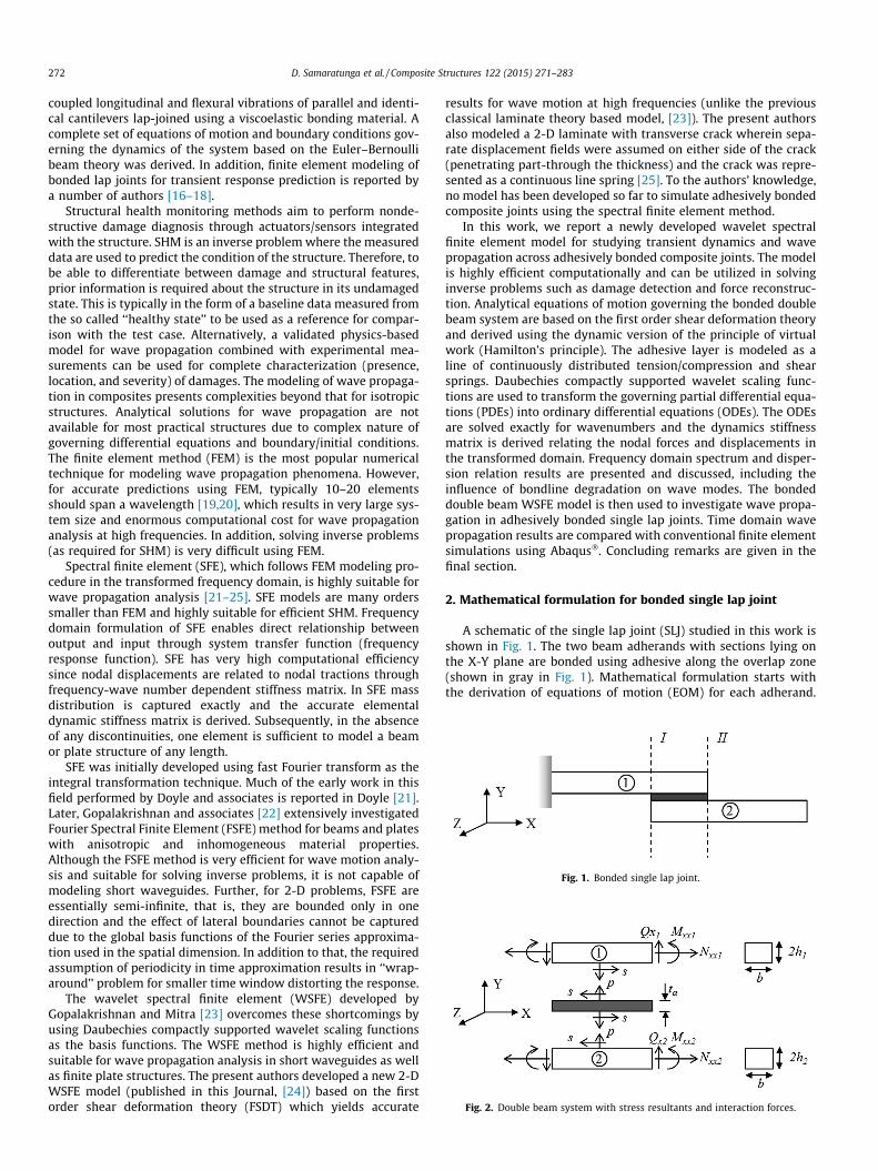
Fig. 1. Bonded single lap joint.

Fig. 2. Double beam system with stress resultants and interaction forces.

272 D. Samaratunga et al. / Composite Structures 122 (2015) 271–283

coupled longitudinal and flexural vibrations of parallel and identi-cal cantilevers lap-joined using a viscoelastic bonding material. Acomplete set of equations of motion and boundary conditions gov-erning the dynamics of the system based on the Euler–Bernoullibeam theory was derived. In addition, finite element modeling ofbonded lap joints for transient response prediction is reported bya number of authors [16–18].

Structural health monitoring methods aim to perform nonde-structive damage diagnosis through actuators/sensors integratedwith the structure. SHM is an inverse problem where the measureddata are used to predict the condition of the structure. Therefore, tobe able to differentiate between damage and structural features,prior information is required about the structure in its undamagedstate. This is typically in the form of a baseline data measured fromthe so called ‘‘healthy state’’ to be used as a reference for compar-ison with the test case. Alternatively, a validated physics-basedmodel for wave propagation combined with experimental mea-surements can be used for complete characterization (presence,location, and severity) of damages. The modeling of wave propaga-tion in composites presents complexities beyond that for isotropicstructures. Analytical solutions for wave propagation are notavailable for most practical structures due to complex nature ofgoverning differential equations and boundary/initial conditions.The finite element method (FEM) is the most popular numericaltechnique for modeling wave propagation phenomena. However,for accurate predictions using FEM, typically 10–20 elementsshould span a wavelength [19,20], which results in very large sys-tem size and enormous computational cost for wave propagationanalysis at high frequencies. In addition, solving inverse problems(as required for SHM) is very difficult using FEM.

Spectral finite element (SFE), which follows FEM modeling pro-cedure in the transformed frequency domain, is highly suitable forwave propagation analysis [21–25]. SFE models are many orderssmaller than FEM and highly suitable for efficient SHM. Frequencydomain formulation of SFE enables direct relationship betweenoutput and input through system transfer function (frequencyresponse function). SFE has very high computational efficiencysince nodal displacements are related to nodal tractions throughfrequency-wave number dependent stiffness matrix. In SFE massdistribution is captured exactly and the accurate elementaldynamic stiffness matrix is derived. Subsequently, in the absenceof any discontinuities, one element is sufficient to model a beamor plate structure of any length.

SFE was initially developed using fast Fourier transform as theintegral transformation technique. Much of the early work in thisfield performed by Doyle and associates is reported in Doyle [21].Later, Gopalakrishnan and associates [22] extensively investigatedFourier Spectral Finite Element (FSFE) method for beams and plateswith anisotropic and inhomogeneous material properties.Although the FSFE method is very efficient for wave motion analy-sis and suitable for solving inverse problems, it is not capable ofmodeling short waveguides. Further, for 2-D problems, FSFE areessentially semi-infinite, that is, they are bounded only in onedirection and the effect of lateral boundaries cannot be captureddue to the global basis functions of the Fourier series approxima-tion used in the spatial dimension. In addition to that, the requiredassumption of periodicity in time approximation results in ‘‘wrap-around’’ problem for smaller time window distorting the response.

The wavelet spectral finite element (WSFE) developed byGopalakrishnan and Mitra [23] overcomes these shortcomings byusing Daubechies compactly supported wavelet scaling functionsas the basis functions. The WSFE method is highly efficient andsuitable for wave propagation analysis in short waveguides as wellas finite plate structures. The present authors developed a new 2-DWSFE model (published in this Journal, [24]) based on the firstorder shear deformation theory (FSDT) which yields accurate

results for wave motion at high frequencies (unlike the previousclassical laminate theory based model, [23]). The present authorsalso modeled a 2-D laminate with transverse crack wherein sepa-rate displacement fields were assumed on either side of the crack(penetrating part-through the thickness) and the crack was repre-sented as a continuous line spring [25]. To the authors’ knowledge,no model has been developed so far to simulate adhesively bondedcomposite joints using the spectral finite element method.

In this work, we report a newly developed wavelet spectralfinite element model for studying transient dynamics and wavepropagation across adhesively bonded composite joints. The modelis highly efficient computationally and can be utilized in solvinginverse problems such as damage detection and force reconstruc-tion. Analytical equations of motion governing the bonded doublebeam system are based on the first order shear deformation theoryand derived using the dynamic version of the principle of virtualwork (Hamilton’s principle). The adhesive layer is modeled as aline of continuously distributed tension/compression and shearsprings. Daubechies compactly supported wavelet scaling func-tions are used to transform the governing partial differential equa-tions (PDEs) into ordinary differential equations (ODEs). The ODEsare solved exactly for wavenumbers and the dynamics stiffnessmatrix is derived relating the nodal forces and displacements inthe transformed domain. Frequency domain spectrum and disper-sion relation results are presented and discussed, including theinfluence of bondline degradation on wave modes. The bondeddouble beam WSFE model is then used to investigate wave propa-gation in adhesively bonded single lap joints. Time domain wavepropagation results are compared with conventional finite elementsimulations using Abaqus�. Concluding remarks are given in thefinal section.

2. Mathematical formulation for bonded single lap joint

A schematic of the single lap joint (SLJ) studied in this work isshown in Fig. 1. The two beam adherands with sections lying onthe X-Y plane are bonded using adhesive along the overlap zone(shown in gray in Fig. 1). Mathematical formulation starts withthe derivation of equations of motion (EOM) for each adherand.

D. Samaratunga et al. / Composite Structures 122 (2015) 271–283 273

The equations of motion of the adherands inside the overlap zone(the area between the dashed lines I and II in Fig. 1) are firstderived using Hamilton’s principle. The adherand portion outsidethe overlap area can be treated as a beam free of external interac-tions and EOM are reduced from the formulation for overlappedregion by relieving adhesive effect.

2.1. Equations for wave motion in adhesively bonded double beamsystem

The free body diagram of the double beam system (representingthe overlap zone of the single lap joint in Fig. 1) is shown in Fig. 2.Normal, shear and bending stress resultants are denoted by Ni, Qi

and Mi, respectively, for each of the beams numbered by i (=1,2).Normal and shear interaction forces between the adherands andthe adhesive layer are given by p and s measured in force per unitlength. Transverse shear in the adhesive layer is assumed to benegligible since its thickness is much smaller than the adherands.The cross sections of the adherands are considered to be rectangu-lar with area A = 2hib.

In a beam, the displacement fields for axial and transversemotion based on FSDT [26] are given by,

uðx; y; tÞ ¼ ucðx; tÞ � y/ðx; tÞvðx; y; tÞ ¼ vcðx; tÞ

ð1Þ

where u and v are axial and transverse displacements, respectively,at any material point on the beam. The terms uc and vc are the beamaxial and transverse displacements along the reference (mid) plane.Anticlockwise rotation of the beam cross-section about Z-axis isgiven by /. Note that the subscript of the terms denoting adherandnumber (appearing in Fig. 2) has been omitted for simplicity. Thederivation of EOM for each of the adherands of the above doublebeam system starts by expressing the strain in terms of the dis-placement field. Once the strains are determined, then virtualkinetic and total potential energies are calculated. According tothe dynamic version of the principle of virtual work (also calledHamilton’s principle) the variation of line integral of the kineticand total potential energy difference, also known as the Lagrangian,between two arbitrary time instants is equal to zero for a conserva-tive body [27]. Thus the Euler–Lagrange EOM for beam adherands,including the effect of adhesive layer, can be derived.

Even though one can use the general nonlinear strain–displace-ment relations, the present work restricts the development tosmall strains and displacements for simplicity since our main focusis WSFE modeling. The linear strains associated with the above dis-placement field (Eq. (1)) are

exx ¼@u@x¼ @uc

@x� y

@/@x

; cxy ¼@v@xþ @u@y¼ @vc

@x� /

eyy ¼ ezz ¼ cxz ¼ cyz ¼ 0 ð2Þ

Total potential energy is the sum of the strain energy andpotential energy due to internal and external forces. For a bodywhose volume is denoted by V, the virtual strain energy can bewritten as

dU ¼Z

VrijdeijdV ð3Þ

where d is the variational operator [27] and rij are stress terms cor-responding to strain terms in Eq. (2). Substituting strains of Eq. (2)into Eq. (3), we get

dU ¼Z L

0

ZA½rxxdexx þ rxydcxy�dAdx

¼Z L

0Nxx

@duc

@x�Mxx

@d/@xþ Qx

@dvc

@x� Q xd/

� �dx ð4Þ

where the force resultants are defined as

Nxx

Mxx

Q x

8><>:9>=>; ¼ b

Z h

�h

rxx

yrxx

rxy

8><>:9>=>;dy; ð5Þ

Here L and b are the length and width of the beam, respectively.Integration by parts is used to relieve variations from any differen-tiation and thus Eq. (4) can be written as

dU ¼ �Z L

0

@Nxx

@xduc �

@Mxx

@xd/þ @Q x

@xdvc þ Q xd/

� �dx

þ Nxxduc½ �L0 � ½Mxxd/�L0 þ ½Q xdvc�L0 ð6Þ

In the absence of body forces, virtual work due to external trac-tions, t; causing virtual displacement, du, over the portion S2 oftotal boundary S can be written as

dV ¼ �Z

S2

t dudS ð7Þ

The external forces on the top adherand are s and p, and the vir-tual work due to external forces can be written as

dV ¼ �Z L

0½sðduc þ d/hÞ � pdvc�dx ð8Þ

The virtual kinetic energy of the body is defined as

dK ¼Z

Vq@u@t� @du@t

dV ð9Þ

where q is the mass density. Upon substitution of the displacementfield given by Eq. (1) into Eq. (9), the virtual kinetic energy, dK , canbe written as

dK ¼Z L

0

Z h

�hqb

@uc

@t� y

@/@t

� �@duc

@t� y

@d/@t

� �þ @vc

@t@dvc

@t

� �dydx

ð10Þ

This expression also contains terms with derivatives of varia-tions. Integration by parts is used to obtain the final form of virtualkinetic energy.

dK¼�Z L

0I0@2uc

@t2 duc� I1@2uc

@t2 d/� I1@2/

@t2 ducþ I2@2/

@t2 d/þ I0@2vc

@t2 dv c

" #dx

þ I0@uc

@tduc

� �L

0� I1

@uc

@td/

� �L

0� I1

@/@t

duc

� �L

0þ I2

@/@t

d/

� �L

0

þ I0@vc

@tdvc

� �L

0

ð11Þ

where the inertial terms are defined as

I0

I1

I2

8><>:9>=>; ¼ qb

Z h

�h

1y

y2

8><>:9>=>;dy; ð12Þ

The inertial term I1 would be zero when the mid plane is takenas the reference. According to Hamilton’s principle the relationshipof kinetic and total potential energies for a conservative elasticbody can be written as

dZ t2

t1

½K � ðU þ VÞ�dt ¼ 0 ð13Þ

where t1 and t2 are two arbitrary time instants. By substituting Eqs.(6), (8) and (11) into Eq. (13) and rearranging the terms, we get


Z t2

t1

Z L

0

@Nxx

@xþs� I0

@2uc

@t2 þ I1@2/

@t2

!ducþ

@Qx

@x�p� I0

@2vc

@t2

!dvc

"(

þ �@Mxx

@xþQxþ

�hsþ I1

@2uc

@t2 �I2@2/

@t2

!d/

#dx

�½Nxxduc�L0þ½Mxxd/�L0�½Q xdv c�L0

)dt ð14Þ

The terms obtained in volume V but evaluated at t1 and t2 wereset to zero because the virtual displacements are zero there (byassumption). The Euler–Lagrange equations for the top adherandbased on FSDT are obtained by setting the coefficients ofduc; dvc and d/ in Eq. (14) to zero:

du1c : @Nxx1@x þ s� I0

@2u1c@t2 þ I1

@2/1@t2 ¼ 0

dv1c : @Qx1@x � p� I0

@2v1c@t2 ¼ 0

d/1 : � @Mxx1@x þ Qx1 þ h1sþ I1

@2u1c@t2 � I2

@2/1@t2 ¼ 0

ð15Þ

Eq. (14) contains the boundary condition terms given by

Nxx1 ¼ Nxx1; Q x1 ¼ Q x1; Mxx1 ¼ �Mxx1 ð16Þ

Similar procedure is followed to obtain EOM and the boundaryconditions for the bottom adherand. The final form of the EOM forthe bottom adherand is

du2c : @Nxx2@x � s� I0

@2u2c@t2 þ I1

@2/2@t2 ¼ 0

dv2c : @Qx2@x þ p� I0

@2v2c@t2 ¼ 0

d/2 : � @Mxx2@x þ Qx2 þ h2sþ I1

@2u2c@t2 � I2

@2/2@t2 ¼ 0

ð17Þ

and the natural boundary conditions for the bottom adherand arewritten as

Nxx2 ¼ Nxx2; Q x2 ¼ Q x2; Mxx2 ¼ �Mxx2 ð18Þ

Subscripts denoting top and bottom adherands are included inEqs. (15)–(18) for clarity. Since the development so far did not uti-lize the constitutive equations, Eqs. (15) and (17) can be tailored toaddress nonlinear elastic body problems by incorporating nonlin-ear strain terms in Eq. (2). However, present work is focused on lin-ear aspect of the problem, as noted earlier. Next, force and momentresultants given in Eq. (5) are related to the strains of the laminatethrough constitutive equations. To this end, it is assumed that eachlayer is orthotropic with respect to its material symmetry lines andobeys the Hook’s law. Then the strain expressions given in Eq. (2)are used to express the above EOM and boundary conditions (Eqs.(15)–(18)) in displacement terms. The EOM of the top adherandexpressed in displacement terms can be written as

A11@2u1c@x2 � B11

@2/1@x2 þ s� I0

@2u1c@t2 þ I1

@2/1@t2 ¼ 0

jA55@2v1c@x2 � @/1

@x

� �� p� I0

@2v1c@t2 ¼ 0

�B11@2u1c@x2 þ D11

@2/1@x2 þ A55

@v1c@x � /1

� þ h1sþ I1

@2u1c@t2 � I2

@2/1@t2 ¼ 0

ð19Þ

The term j is the shear correction factor which is introduced tomitigate the constant transverse strain state assumed by the FSDT[26]. The boundary conditions can be written as

Nxx1 ¼ A11@u1c

@x� B11

@/1

@x; Qx1 ¼ jA55

@v1c

@x� /1

� �;

Mxx1 ¼ �B11@u1c

@xþ D11

@/1

@xð20Þ

Similarly, the EOM for the bottom adherand in displacementterms can be written as

A11@2u2c@x2 � B11

@2/2@x2 � s� I0

@2u2c@t2 þ I1

@2/2@t2 ¼ 0

jA55@2v2c@x2 � @/2

@x

� �þ p� I0

@2v2c@t2 ¼ 0

�B11@2u2c@x2 þ D11

@2/2@x2 þ A55

@v2c@x � /2

� þ h2sþ I1

@2u2c@t2 � I2

@2/2@t2 ¼ 0

ð21Þ

The boundary conditions can be written as

Nxx2 ¼ A11@u2c

@x� B11

@/2

@x; Q x2 ¼ jA55

@v2c

@x� /2

� �;

Mxx2 ¼ �B11@u2c

@xþ D11

@/2

@xð22Þ

The axial, axial-bending, and bending stiffness terms appearingin the formulation are defined as

A11 ¼ bXNp

k¼1

Q ðkÞ11 ykþ1 � yk

� ; B11 ¼

12

bXNp

k¼1

Q ðkÞ11 y2kþ1 � y2

k

� ;

D11 ¼13

bXNp

k¼1

Q ðkÞ11 y3kþ1 � y3

k

� ð23Þ

where Q ðkÞ11 represents the stiffness of the kth ply of the laminate[26] and Np is the total number of plies. The two sets of EOM givenby Eqs. (19) and (21) are coupled due to the presence of normal andshear forces (p and s) at the adhesive and adherand interfaces. Bysetting these adhesive-adherand interaction forces to zero in oneset of the equations, EOM for a simple beam (that is, in the absenceof distributed external forces) can be recovered. These forces can bederived through constitutive relations of the adhesive layer. Theconstitutive relations for the adhesive layer are established usingtwo parameter elastic foundation approach, where the adhesivelayer is assumed to be composed of continuously distributed shearand tension/compression springs. Similar approach has been takenby Mortensen [28] for solving static problems and by Saito and Tani[15] for studying coupled longitudinal and flexural vibrations ofadhesively bonded joints. From Fig. 2, the interaction forces p ands are found to be

s ¼ ksðu2c � h2/2 � u1c � h1/1Þ; ks ¼Ga

ta;

p ¼ ktðv1c � v2cÞ; kt ¼Ea

tað24Þ

where Ea and Ga are Young’s and shear moduli, respectively. Theterms ks and kt are spring constants into X and Y directions. Thiscompletes the derivation of partial differential equations for thebonded double beam system shown in Fig. 2. It should be men-tioned that the procedure outlined above can be used to formulateEOMs for other bonded structures (with larger number of mem-bers), such as a double lap joint. As already mentioned, the govern-ing differential Eqs. (19) and (21) represent a system of coupledlinear partial differential equations (PDEs), which are difficult tosolve exactly in the time domain for all boundary conditions. Herewe employ WSFE method to solve the governing PDEs in the fre-quency domain. The solution for given loading and boundary condi-tions is obtained in the frequency domain and inverse wavelettransform is performed to obtain time domain results. The next sec-tion describes the implementation of WSFE method for solvingEOMs presented above.

2.2. Wavelet approximation of governing equations

The WSFE formulation begins with transformation of the fieldvariables (displacements) into the frequency domain using thewavelet transform. Daubechies compactly supported wavelet scal-ing functions [29] are used for approximation in time, which

Fig. 3. Nodal representation of the spectral element for the bonded double beamsystem.


reduces the PDEs to ODEs in the spatial dimension. Compactly sup-ported scaling functions have only a finite number of filter coeffi-cients with non-zero values, which enables easy handling offinite geometries and imposition of boundary conditions. Mitraand Gopalakrishnan [30] provide a complete prescription of theuse of Daubechies compactly supported wavelets for solving 1-Dwave equations. The steps involved in the WSFE method are brieflydescribed here; readers interested in further details may refer to[23,30].

Let the time–space displacement variable u(x, t) be discretizedat n points in the time window (0, tf) and s = 0, 1,...,n�1 be thesampling points, then t ¼ Dts where Dt is the time intervalbetween two sampling points. The function u(x, t) can be approxi-mated at an arbitrary scale as

uðx; tÞ ¼ uðx; sÞ ¼X

k

ukðxÞuðs� kÞ; k 2 Z ð25Þ

where ukðxÞ are the approximation coefficients at a certain spatialdimension and uðsÞ are scaling functions associated with Daube-chies wavelets. The other translational and rotational displace-ments v(x,y,t) and /ðx; y; tÞ are approximated similarly. Bysubstituting these approximations into the first equation of Eq.(19) we get

A11

Xk

d2uk

dx2 uðs� kÞ � B11

Xk

@2/k

@x2 uðs� kÞ þX

k

skuðs� kÞ

� I0

Dt2

Xk

uku00ðs� kÞ þ I1

Dt2

Xk

/ku00ðs� kÞ ¼ 0 ð26Þ

Here the subscripts denoting the adherand have been droppedagain for simplified notation although the terms represent midplane displacements of the top adherand. Taking inner product onboth sides of Eq. (26) with translations of the scaling function(uðs� jÞ for j = 1,2, . . .,n-1) and using the orthogonal property ofDaubechies scaling function results in the cancelation of all theterms except when j = k and yields n simultaneous equations. ThusEq. (26) reduces to

A11d2uj

dx2 � B11@2/j

@x2 þ sj �1

Dt2

XjþN�2

k¼j�Nþ2

X2j�kðI0uk � I1/kÞ ¼ 0;

j ¼ 0;1;2; . . . ;n� 1 ð27Þ

where N is the order of the Daubechies wavelet and X2j�k are the

connection coefficients. For compactly supported wavelets, X2j�k

are nonzero only in the interval k = j � N + 2 to k = j + N � 2. A com-plete description for the evaluation of connection coefficients of dif-ferent orders of derivative is given in [31]. It can be observed in theODEs of Eq. (27) that certain coefficients uj near the vicinity of theboundaries (j = 0 and j = n � 1) lie outside the time window [0, tf]defined by j = 0, 1, ..., n � 1. Therefore it is necessary to treat theboundaries appropriately. Among several methods available [23],we use wavelet extrapolation technique [32] for solving the bound-ary value problem for aperiodic boundaries. This approach allows

treatment of finite length data and uses polynomial to extrapolatecoefficients at boundaries either from interior coefficients or bound-ary values. The method is particularly suitable for approximation intime for the ease of initial value imposition. After treating theboundaries using wavelet extrapolation technique, the ODEs inEq. (27) can be written in matrix form as

A11d2uj

dx2

( )� B11

@2/j

@x2

( )þ fsjg � I0½C1�2uj þ I1½C1�2/j ¼ 0 ð28Þ

where ½C1�2 is the first order connection coefficient matrix. Next, thecoupled ODEs in Eq. (28) are decoupled using eigenvalue analysis ofC1 given by

C1 ¼ UPU�1 ð29Þ

where P is the diagonal matrix with eigenvalues and U is the eigen-vectors matrix of C1. By letting the eigenvalues be �icj ði ¼

ffiffiffiffiffiffiffi�1p

Þ,the final decoupled form of the reduced ODEs given in Eq. (29)can be written as

A11d2uj

dx2 � B11d2/j

dx2 þ sj þ I0c2j uj � I1c2

j /j ¼ 0 ð30Þ

where uj is defined as uj ¼ U�1uj. It should be mentioned here thatthe sampling rate Dt should be less than a certain value to avoidspurious dispersion in simulations using WSFE. In Mitra and Gopal-akrishnan [33], a numerical study has been conducted from whichthe required Dt can be determined depending on the order N ofthe Daubechies scaling function and frequency content of the inputload.

The governing PDEs for each adherand are transformed follow-ing similar steps as in Eqs. (25)–(30). For further steps, the sub-script j (of Eq. (30)) is dropped for simplified notations and all ofthe following equations are valid for j = 0,1, ...,n � 1. Also the sub-scripts denoting the adherand number is reintroduced for easy ref-erence. Following these, the transformed governing ODEs for thetop adherand are written as

A11d2 u1c

dx2 � B11d2/1

dx2 þ sþ I0c2u1c þ I1c2/1 ¼ 0

jA55ðd2 v1c

dx2 � d/1dx Þ � pþ I0c2v1c ¼ 0

�B11d2u1c

dx2 þ D11d2/1

dx2 þ A55dv1c

dx � /1

� �þ h1s� I1c2u1c þ I2c2/1 ¼ 0

ð31Þ

Similarly the governing PDEs for the bottom adherand take theform

A11d2 u2c

dx2 � B11d2/2

dx2 � sþ I0c2u2c þ I1c2/2 ¼ 0

jA55d2v2c

dx2 � d/2dx

� �þ pþ I0c2v2c ¼ 0

�B11d2u2c

dx2 þ D11d2/2

dx2 þ A55dv2c

dx � /2

� �þ h2s� I1c2u2c þ I2c2/2 ¼ 0

ð32Þ

and the transformed boundary conditions for the two adherandsare,bNxx1 ¼ A11

du1c

dx� B11

d/1

dx;

bQ x1 ¼ jA55dv1c

dx� /1

� �;

cMxx1 ¼ �B11du1c

dxþ D11

d/1

dxbNxx2 ¼ A11

du2c

dx� B11

d/2

dx;

bQ x2 ¼ jA55dv2c

dx� /2

� �;cMxx2 ¼ �B11

du2c

dxþ D11

d/2

dxð33Þ

Once the ODEs are derived for the beam adherands the nextstep is to compute wavenumbers and wave amplitudes whichare used in deriving shape functions of the spectral element.

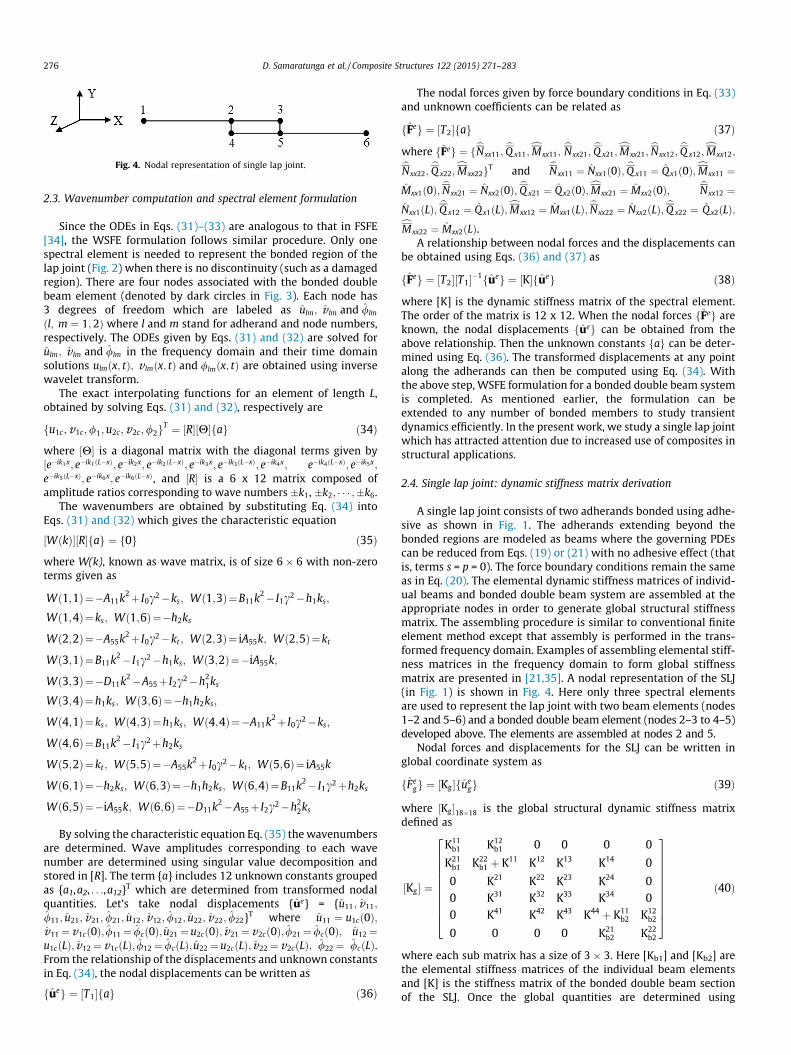
Fig. 4. Nodal representation of single lap joint.


2.3. Wavenumber computation and spectral element formulation

Since the ODEs in Eqs. (31)–(33) are analogous to that in FSFE[34], the WSFE formulation follows similar procedure. Only onespectral element is needed to represent the bonded region of thelap joint (Fig. 2) when there is no discontinuity (such as a damagedregion). There are four nodes associated with the bonded doublebeam element (denoted by dark circles in Fig. 3). Each node has3 degrees of freedom which are labeled as ulm; v lm and /lm

ðl; m ¼ 1;2Þ where l and m stand for adherand and node numbers,respectively. The ODEs given by Eqs. (31) and (32) are solved forulm; v lm and /lm in the frequency domain and their time domainsolutions ulmðx; tÞ; v lmðx; tÞ and /lmðx; tÞ are obtained using inversewavelet transform.

The exact interpolating functions for an element of length L,obtained by solving Eqs. (31) and (32), respectively are

fu1c;v1c;/1;u2c;v2c;/2gT ¼ ½R�½H�fag ð34Þ

where ½H� is a diagonal matrix with the diagonal terms given by½e�ik1x; e�ik1ðL�xÞ; e�ik2x; e�ik2ðL�xÞ; e�ik3x; e�ik3ðL�xÞ; e�ik4x; e�ik4ðL�xÞ; e�ik5x;

e�ik5ðL�xÞ; e�ik6x; e�ik6ðL�xÞ, and ½R� is a 6 x 12 matrix composed ofamplitude ratios corresponding to wave numbers �k1, �k2; � � � ;�k6.

The wavenumbers are obtained by substituting Eq. (34) intoEqs. (31) and (32) which gives the characteristic equation

½WðkÞ�½R�fag ¼ f0g ð35Þ

where W(k), known as wave matrix, is of size 6 � 6 with non-zeroterms given as

Wð1;1Þ¼�A11k2þ I0c2�ks; Wð1;3Þ¼B11k2� I1c2�h1ks;

Wð1;4Þ¼ks; Wð1;6Þ¼�h2ks

Wð2;2Þ¼�A55k2þ I0c2�kt ; Wð2;3Þ¼ iA55k; Wð2;5Þ¼kt

Wð3;1Þ¼B11k2� I1c2�h1ks; Wð3;2Þ¼�iA55k;

Wð3;3Þ¼�D11k2�A55þ I2c2�h21ks

Wð3;4Þ¼h1ks; Wð3;6Þ¼�h1h2ks;

Wð4;1Þ¼ks; Wð4;3Þ¼h1ks; Wð4;4Þ¼�A11k2þ I0c2�ks;

Wð4;6Þ¼B11k2� I1c2þh2ks

Wð5;2Þ¼kt ; Wð5;5Þ¼�A55k2þ I0c2�kt ; Wð5;6Þ¼ iA55k

Wð6;1Þ¼�h2ks; Wð6;3Þ¼�h1h2ks; Wð6;4Þ¼B11k2� I1c2þh2ks

Wð6;5Þ¼�iA55k; Wð6;6Þ¼�D11k2�A55þ I2c2�h22ks

By solving the characteristic equation Eq. (35) the wavenumbersare determined. Wave amplitudes corresponding to each wavenumber are determined using singular value decomposition andstored in [R]. The term {a} includes 12 unknown constants groupedas {a1,a2, . . .,a12}T which are determined from transformed nodalquantities. Let’s take nodal displacements {ue} = {u11; v11;

/11; u21; v21; /21; u12; v12; /12; u22; v22; /22}T where u11 ¼ u1cð0Þ;v11¼v1cð0Þ; /11¼ /cð0Þ; u21 ¼u2cð0Þ; v21¼v2cð0Þ;/21¼ /cð0Þ; u12¼u1cðLÞ; v12¼v1cðLÞ; /12¼ /cðLÞ; u22¼u2cðLÞ; v22¼v2cðLÞ; /22¼ /cðLÞ.From the relationship of the displacements and unknown constantsin Eq. (34), the nodal displacements can be written as

fueg ¼ ½T1�fag ð36Þ

The nodal forces given by force boundary conditions in Eq. (33)and unknown coefficients can be related as

fFeg ¼ ½T2�fag ð37Þ

where fFeg ¼ fbNxx11;bQ x11;

cMxx11;bNxx21;

bQ x21;cMxx21;

bNxx12;bQ x12;

cMxx12;bNxx22;bQ x22;

cMxx22gT and bNxx11 ¼ Nxx1ð0Þ; bQ x11 ¼ Q x1ð0Þ;cMxx11 ¼

Mxx1ð0Þ; bNxx21 ¼ Nxx2ð0Þ; bQ x21 ¼ Q x2ð0Þ;cMxx21 ¼ Mxx2ð0Þ; bNxx12 ¼

Nxx1ðLÞ; bQ x12 ¼ Q x1ðLÞ;cMxx12 ¼ Mxx1ðLÞ; bNxx22 ¼ Nxx2ðLÞ; bQ x22 ¼ Q x2ðLÞ;cMxx22 ¼ Mxx2ðLÞ.A relationship between nodal forces and the displacements can

be obtained using Eqs. (36) and (37) as

fFeg ¼ ½T2�½T1��1fueg ¼ ½K�fueg ð38Þ

where [K] is the dynamic stiffness matrix of the spectral element.The order of the matrix is 12 x 12. When the nodal forces fFeg areknown, the nodal displacements fueg can be obtained from theabove relationship. Then the unknown constants fag can be deter-mined using Eq. (36). The transformed displacements at any pointalong the adherands can then be computed using Eq. (34). Withthe above step, WSFE formulation for a bonded double beam systemis completed. As mentioned earlier, the formulation can beextended to any number of bonded members to study transientdynamics efficiently. In the present work, we study a single lap jointwhich has attracted attention due to increased use of composites instructural applications.

2.4. Single lap joint: dynamic stiffness matrix derivation

A single lap joint consists of two adherands bonded using adhe-sive as shown in Fig. 1. The adherands extending beyond thebonded regions are modeled as beams where the governing PDEscan be reduced from Eqs. (19) or (21) with no adhesive effect (thatis, terms s = p = 0). The force boundary conditions remain the sameas in Eq. (20). The elemental dynamic stiffness matrices of individ-ual beams and bonded double beam system are assembled at theappropriate nodes in order to generate global structural stiffnessmatrix. The assembling procedure is similar to conventional finiteelement method except that assembly is performed in the trans-formed frequency domain. Examples of assembling elemental stiff-ness matrices in the frequency domain to form global stiffnessmatrix are presented in [21,35]. A nodal representation of the SLJ(in Fig. 1) is shown in Fig. 4. Here only three spectral elementsare used to represent the lap joint with two beam elements (nodes1–2 and 5–6) and a bonded double beam element (nodes 2–3 to 4–5)developed above. The elements are assembled at nodes 2 and 5.

Nodal forces and displacements for the SLJ can be written inglobal coordinate system as

fFegg ¼ ½Kg �fue

gg ð39Þ

where ½Kg �18�18 is the global structural dynamic stiffness matrixdefined as

½Kg � ¼

K11b1 K12

b1 0 0 0 0

K21b1 K22

b1 þ K11 K12 K13 K14 0

0 K21 K22 K23 K24 00 K31 K32 K33 K34 00 K41 K42 K43 K44 þ K11

b2 K12b2

0 0 0 0 K21b2 K22

b2

26666666664

37777777775ð40Þ

where each sub matrix has a size of 3 � 3. Here [Kb1] and [Kb2] arethe elemental stiffness matrices of the individual beam elementsand [K] is the stiffness matrix of the bonded double beam sectionof the SLJ. Once the global quantities are determined using


Eq. (39) the local displacements can be obtained using respectivenodal quantities and elemental shape functions.

3. Results and discussion

The WSFE model developed above is used for frequency andtime domain wave propagation behavior analysis of composite sin-gle lap joints. Frequency domain spectrum and dispersion relationsare investigated first. Thereafter, time domain wave propagationresults are compared with conventional finite element simulationsperformed using commercial FE software Abaqus� [36]. Examplelap joints are made up of AS4/3501-6 graphite-epoxy compositewith layup sequence as specified in each case. Each of the beamadherands has a depth of h1 = h2 = 0.01 m and width ofb = 0.02 m. Lamina properties are as follows: E1 = 144.48 GPa,E2 = E3 = 9.63 GPa, G23 = G13 = G12 = 4.128 GPa, m23 = 0.3, m13 = m12 =0.02, and q = 1389 kgm�3. Epoxy based structural paste adhesiveHysol EA 9394 with Young’s modulus and Poison’s ratio of4.24 GPa and 0.45, respectively, is taken as the bondline material.The bondline thickness ta = 0.005 m unless specified otherwise.Shear correction factor j appearing in the formulation is taken as5/6 in all the examples. The order of Daubechies scaling functionused is N = 22, if not mentioned specifically.

3.1. Wave propagation: spectrum and dispersion relations

In order to understand the wave propagation behavior ofbonded joints it is important to get an insight of frequency depen-dent wave parameters, spectrum and dispersion relations, whichare readily available in the WSFE method. WSFE can be used toobtain the frequency dependent wave characteristics up to a frac-tion of Nyquist frequency where the fraction is dependent on theorder of the Daubechies wavelet used. In order to be able to useWSFE in frequency domain analysis the boundaries arising fromfinite data lengths need to be treated as periodic. For further details

Fig. 5. Spectrum relations for bonded double beam with l

of the use of WSFE for studying frequency dependent wave charac-teristics, readers may refer to [23,33].

For studying wave propagation in bonded single lap joint, it isnecessary to treat the overlapped region and the rest separately.Wave motion of the adherands outside the overlap region is gov-erned by Eq. (15) without the bondline effects. Mahapatra andGopalakrishnan [34] discuss the wave propagation behavior ofsuch standalone beams (also referred to as single beams elsewherein the menuscript) in detail. Therefore we focus here on the over-lapped region or bonded double beam region of the joint. There aresix modes associated with bonded double beam system where thecharacteristic equation is given by Eq. (35). The wavenumbers arecomputed by setting the determinant of the wave matrix ðjWðkÞjÞto zero. The resulting 12th order characteristic equation is verycomplex and cumbersome to solve analytically. Here the compan-ion matrix method is used to solve the characteristic equationwhere the roots are determined as eigenvalues of the companionmatrix. Once the eigenvalues are obtained they can be used toobtain eigenvectors using singular value decomposition [22]. Somea priori tests can be performed on the characteristic equation inorder to get an idea about the presence of propagating and evanes-cent modes as well as cutoff frequencies. By setting the frequencyðcÞ to zero and solving the characteristic equation for wavenum-bers (k), it can be observed that for the uncoupled case (Bij = 0)there are three imaginary wavenumbers corresponding to threeevanescent modes. The cutoff frequencies (where the evanescentmodes turn into propagating modes) can be evaluated using thecharacteristic equation by setting k = 0 and solving for frequency.

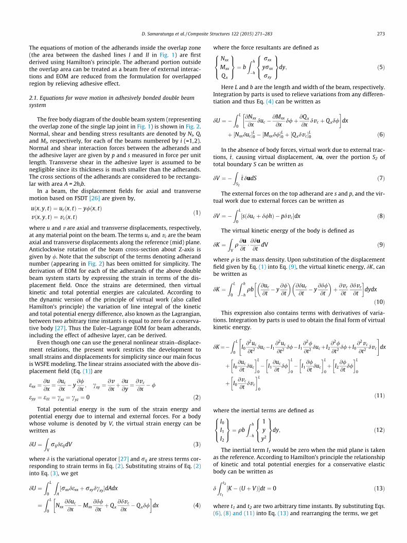
Fig. 5 shows the spectrum relations of bonded double beamwith layup sequence of [0]10 for each adherand. This relationshipis obtained by solving the characteristic equation with a samplingtime of Dt ¼ 0:1 ls: Real and imaginary wavenumbers are plottedalong positive and negative Y-axis, respectively. There are threemodes with zero wavenumber values at zero frequency, (c ¼ 0),meaning none of these three will propagate at that frequency.These fundamental modes resemble axial, flexural and shear

ayup sequence of [0]10 (zoomed image on the right).

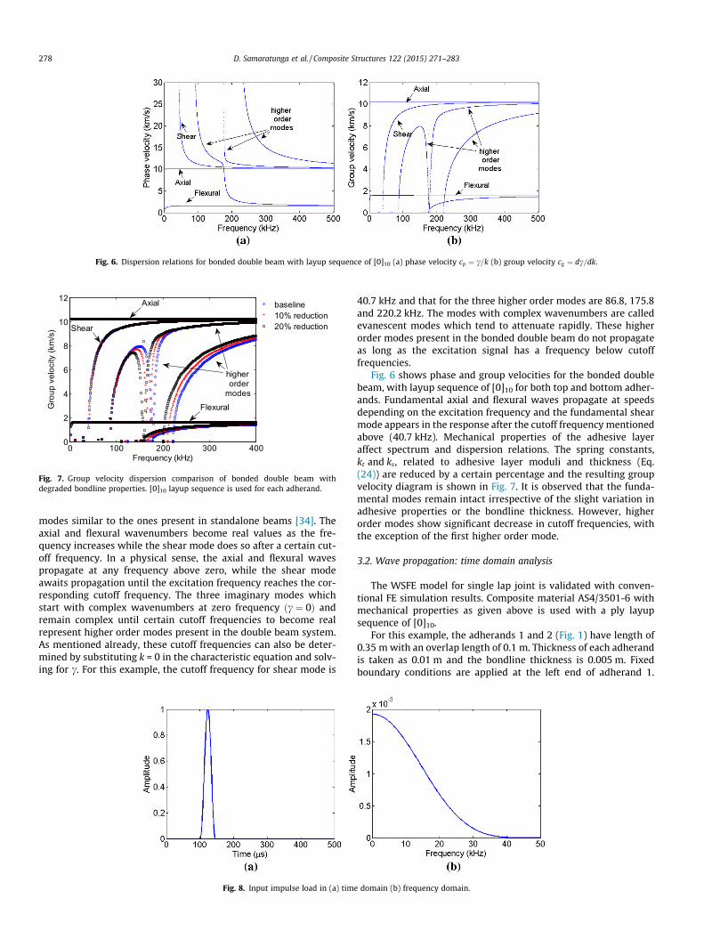
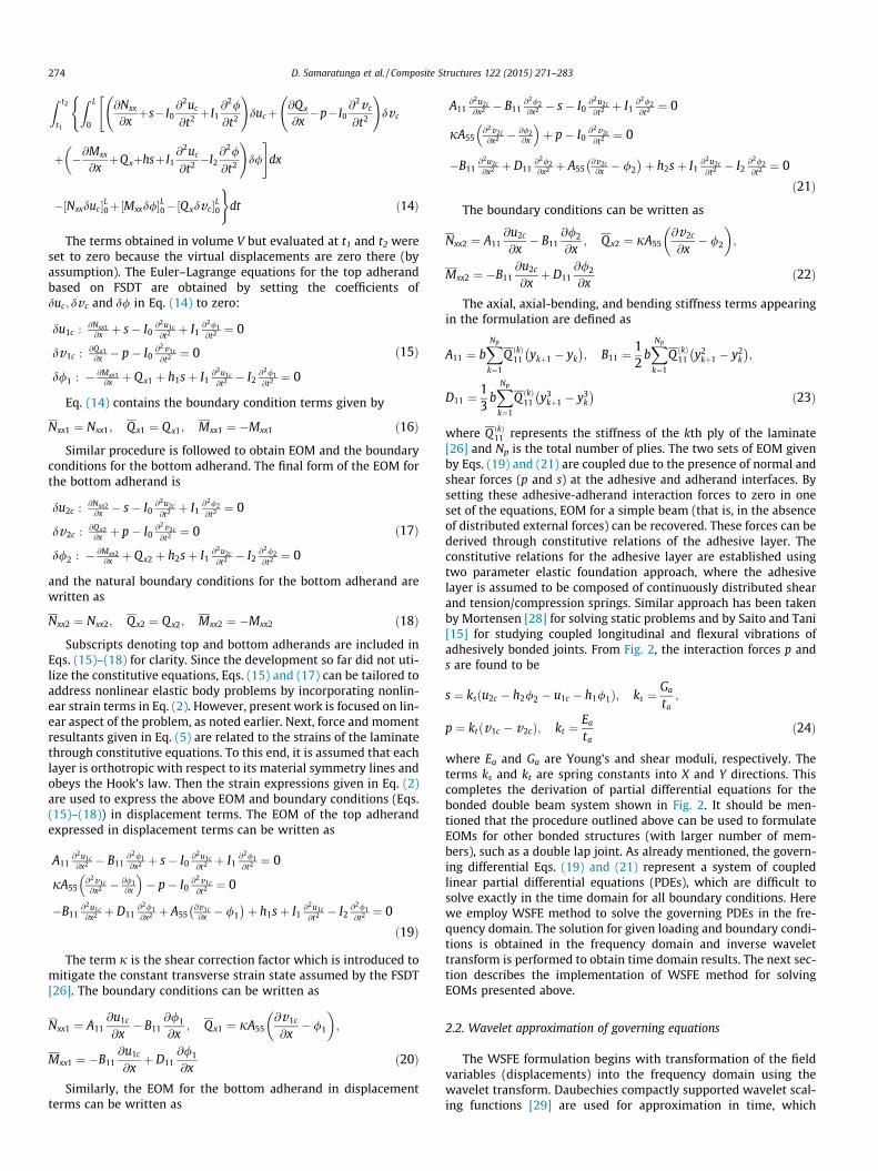
Fig. 6. Dispersion relations for bonded double beam with layup sequence of [0]10 (a) phase velocity cp ¼ c=k (b) group velocity cg ¼ dc=dk.

0 100 200 300 4000

2

4

6

8

10

12

Frequency (kHz)

Gro

up v

eloc

ity (k

m/s

)

baseline10% reduction20% reduction

higher order

modesFlexural

Axial

Shear

Fig. 7. Group velocity dispersion comparison of bonded double beam withdegraded bondline properties. [0]10 layup sequence is used for each adherand.


modes similar to the ones present in standalone beams [34]. Theaxial and flexural wavenumbers become real values as the fre-quency increases while the shear mode does so after a certain cut-off frequency. In a physical sense, the axial and flexural wavespropagate at any frequency above zero, while the shear modeawaits propagation until the excitation frequency reaches the cor-responding cutoff frequency. The three imaginary modes whichstart with complex wavenumbers at zero frequency ðc ¼ 0Þ andremain complex until certain cutoff frequencies to become realrepresent higher order modes present in the double beam system.As mentioned already, these cutoff frequencies can also be deter-mined by substituting k = 0 in the characteristic equation and solv-ing for c. For this example, the cutoff frequency for shear mode is

Fig. 8. Input impulse load in (a) time

40.7 kHz and that for the three higher order modes are 86.8, 175.8and 220.2 kHz. The modes with complex wavenumbers are calledevanescent modes which tend to attenuate rapidly. These higherorder modes present in the bonded double beam do not propagateas long as the excitation signal has a frequency below cutofffrequencies.

Fig. 6 shows phase and group velocities for the bonded doublebeam, with layup sequence of [0]10 for both top and bottom adher-ands. Fundamental axial and flexural waves propagate at speedsdepending on the excitation frequency and the fundamental shearmode appears in the response after the cutoff frequency mentionedabove (40.7 kHz). Mechanical properties of the adhesive layeraffect spectrum and dispersion relations. The spring constants,kt and ks, related to adhesive layer moduli and thickness (Eq.(24)) are reduced by a certain percentage and the resulting groupvelocity diagram is shown in Fig. 7. It is observed that the funda-mental modes remain intact irrespective of the slight variation inadhesive properties or the bondline thickness. However, higherorder modes show significant decrease in cutoff frequencies, withthe exception of the first higher order mode.

3.2. Wave propagation: time domain analysis

The WSFE model for single lap joint is validated with conven-tional FE simulation results. Composite material AS4/3501-6 withmechanical properties as given above is used with a ply layupsequence of [0]10.

For this example, the adherands 1 and 2 (Fig. 1) have length of0.35 m with an overlap length of 0.1 m. Thickness of each adherandis taken as 0.01 m and the bondline thickness is 0.005 m. Fixedboundary conditions are applied at the left end of adherand 1.

domain (b) frequency domain.

Fig. 9. (a) Transverse (b) axial response of the single lap joint for transverse impulse input load applied and measured at the free end.

Fig. 10. (a) Transverse response for single lap joint measured at far end of thebonded region due to transversely applied impulse input load at the free end.


Impulse load with a frequency content of 44 kHz (Fig. 8) is appliedat the free end of adherand 2. The single lap joint is modeled inWSFE using two beam elements and one double beam elementdeveloped in this work. Abaqus� model for the SLJ is meshed with5700, 2D plane stress elements with 8 elements along the thick-ness of each adherand. Adhesive bondline consists of 100 elements

Fig. 11. (a) Axial (b) transverse response for single lap joint for ax

(one element along the thickness) with isotropic properties (HysolEA 9394) as specified above. FE simulations are performed usingAbaqus� Explicit dynamic solver. Fig. 9 shows the transverse andaxial response comparisons for the impulse input load applied intotransverse direction. Here we can see that WSFE and FE (Abaqus�)predictions are in very good agreement. Transverse response at theexcitation location (Fig. 9 (a)) shows peak 1 as the excitation inputand peak 2 is the reflection from the overlap boundary (interface IIin Fig. 1). Once the transmitted waves enter the overlapped area,another boundary (interface I in Fig. 1) causes partial reflectionshown as peak 3. Due to the complicated nature of the boundariesin the overlapped area partial reflections and transmissions areobserved repeatedly. The largest response appearing after peak 3is the reflection from the fixed boundary located at far left end ofthe SLJ.

Although the individual adherands consist of symmetric bal-anced layup, wave propagation across the lap joint exhibits axial-transverse coupling. It means that both axial and flexural wavesare generated irrespective of the input excitation direction. Fig. 9(b) shows the axial response measured at the free end of adherand2 (Fig. 1) for a transversely excited impulse input.

Since the adherand laminates are symmetric and balanced, nocoupling exists as long as the wave is propagated through stand-alone beam. Once the flexural wave reaches the overlapped regionboundary (interface II in Fig. 1), it undergoes mode conversionresulting in axial wave propagation. This mode converted andreflected wave (peak 1 in Fig. 9 (b)) reaches the free end first, fol-lowed by wave reflections from boundary at the far end of the

ial impulse input load applied and measured at the free end.

Fig. 12. Axial response of the lap joint measured at far end of the bonded region dueto axially applied impulse input load at the free end.

Fig. 13. Semi-infinite bonded double beam for studying wave propagation indifferent modes.


overlapped region and the fixed boundary. The transverse velocityresponse of the top adherand (adherand 1 in Fig. 1) measured atthe far end of the overlapped region (interface I in Fig. 1) for thesame input is shown in Fig. 10. Here also the WSFE prediction isin very good agreement with FE (Abaqus�) results. All the trans-verse response results (Figs. 9 and 10) are obtained from a singlesimulation performed in a computer with Intel� Core™ i7-3770(3.40 GHz) processor. Computational times taken to completeanalysis for WSFE and Abaqus� (explicit solver) are recorded as3.81 s and 74 s, respectively. It can be noticed that there is a signif-icant reduction in computation time for WSFE when comparedwith conventional FE (explicit) analysis. Authors’ previous studies

( )2mdΔ =

( )4mdΔ =

Fig. 14. Axial and transverse velocity responses measured at 2 m and 4

[24,25] compared simulations times of Abaqus� with standard sol-ver and observed over two orders of magnitude reduction in com-putation time when compared with WSFE. Fig. 11 shows the axialand transverse response comparisons for an axial impulse inputload. For this example the lengths of adherands 1 and 2 areextended to 1.5 m and 1.0 m, respectively, with 0.5 m bondlinelength in order to clearly visualize high velocity axial wave reflec-tions from each boundary. Again, it is observed that WSFE predic-tions are in very good agreement with FE results. We have alreadyobserved through group velocity dispersion diagrams that the axialwaves are non-dispersive. Fig. 11(a) shows that reflected wave-forms preserve their shape irrespective of the propagation lengths,which is a major feature of non-dispersive signals in time domain.In the axial response shown, peak 1 is input load and peak 2 is thefixed boundary reflection. The smaller amplitude peaks betweenthose two are created by boundaries in the overlapped region. Sim-ilar to the observations made in the previous example (Fig. 9),mode converted transverse waves are reflected as shown inFig. 11 (b). Due to the longer wave guide and considerably smallergroup velocity the mode converted transverse response reachesthe free end at a much later time. The axial velocity response ofthe top adherand (adherand 1 in Fig. 1) measured at the far endof the overlapped region (interface I in Fig. 1) for the same axialinput at free end is shown in Fig. 12. Here too the WSFE predictionis in very good agreement with FE (Abaqus�) results.

3.3. Coupled wave propagation in bonded double beam system

Examination of Eq. (35) indicates that wave propagation acrossthe bonded double beam system is coupled in nature, which leadsto propagation of multimodal waves for a given input load. Fig. 13shows the semi-infinite double beam considered in this study inorder to understand the presence of these modes. Here the inputtone burst with 250 kHz central frequency is applied at the freeend of the beam (nodes n1, n2 in Fig. 13). This frequency is selectedsince all the modes present in the double beam system are propa-gating modes at this frequency. The beam is modeled using semi-infinite or throw-off elements available in spectral finite elementanalysis. Hence, there are no boundary reflections present in theresponse which makes the signal analysis and interpretation lesscomplicated. In reality, this beam configuration corresponds to avery long cantilever beam whose response at the said locationsdoes not contain any fixed boundary reflections inside the timewindow of interest. Studying wave propagation using semi-infiniteor throw-off elements is fairly straight forward using the spectralfinite element method as reported previously [21,22]. Similar

( )2mdΔ =

( )4mdΔ =

m away from the free end for axial input load (250 kHz toneburst).

( )2mdΔ =

( )4mdΔ =

( )2mdΔ =

( )4mdΔ =

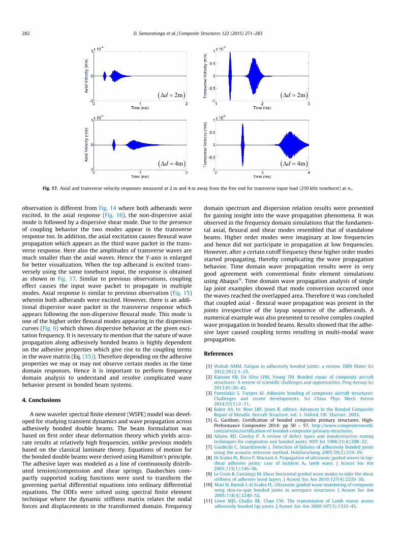
Fig. 15. Axial and transverse velocity responses measured at 2 m and 4 m away from the free end for transverse input load (250 kHz toneburst).


approach is used here in order to model the semi-infinite beamwithout repeating the formulation. Use of this throw-off elementat the structural boundary amounts to absorption of all the energyfrom the structure and hence maximum damping artificially to theresponse. In the examples, the order of Daubechies scaling functionused for time approximation is set to be N = 36 and all otherparameters are same as above examples.

The modes that may appear in the time domain responses isdependent on the nature of loading conditions as well. Thereforethe toneburst input load is first applied at both nodes (n1,n2 inFig. 13) into axial and transverse (X and Y) directions. Theresponses are recorded at a distance ðDd ¼Þ 2 and 4 m away fromthe excitation location (free end) along the beam length. Fig. 14shows the axial and transverse responses recorded at the said loca-tions for an axial input. Here the axially excited toneburst travelsnon-dispersively and no coupling exists (no transverse responseis observed). However, when the beam is excited transversely theaxial-flexural coupling comes into effect as shown in Fig. 15. Herethe amplitudes of wave packets appeared in axial response is muchsmaller than that of flexural wave. Therefore the Y-axis scale iszoomed in by one order of magnitude compared to the flexuralresponse scale. Presence of adhesive layer leads to this coupling

( )2mdΔ =

( )4mdΔ =

Fig. 16. Axial and transverse velocity responses measured at 2 m and 4 m

behavior which causes wave propagation in multiple modes. Inthe axial response the first wave packet is an axial mode and thesecond wave packet is a shear mode. According to the group veloc-ity dispersion curves for the bonded double beam system (Fig. 6)the axial and shear modes have higher group velocities (whichare close to each other in magnitude) compared to the flexuralmode. The axial and flexural modes are non-despersive while theshear mode displays dispersive behavior at this excitation fre-quency. Therefore the shear mode is dispersed continuously as itpropagates along the beam while the other two modes retain theirwave shape.

As mentioned previously, the coupling behavior is also depen-dent on the input loading conditions. To investigate this effectthe input tone burst with 250 kHz central frequency is applied toone of the beams only and the resulting wave propagation on thetop beam is studied. Excitation given to one adherand resultingin wave propagation in the other adherand simulates single lapjoints, which is very important from practical applications pointof view. Figs. 16 and 17 show the axial and transverse responsesfor the input load applied to node n1.

The presence of axial-flexural modes is observed even when theexcitation is given axially into only one of the two beams. This

( )2mdΔ =

( )4mdΔ =

away from the free end for axial input load (250 kHz toneburst) at n1.

( )2mdΔ =

( )4mdΔ =

( )2mdΔ =

( )4mdΔ =

Fig. 17. Axial and transverse velocity responses measured at 2 m and 4 m away from the free end for transverse input load (250 kHz toneburst) at n1.


observation is different from Fig. 14 where both adherands wereexcited. In the axial response (Fig. 16), the non-dispersive axialmode is followed by a dispersive shear mode. Due to the presenceof coupling behavior the two modes appear in the transverseresponse too. In addition, the axial excitation causes flexural wavepropagation which appears as the third wave packet in the trans-verse response. Here also the amplitudes of transverse waves aremuch smaller than the axial waves. Hence the Y-axis is enlargedfor better visualization. When the top adherand is excited trans-versely using the same toneburst input, the response is obtainedas shown in Fig. 17. Similar to previous observations, couplingeffect causes the input wave packet to propagate in multiplemodes. Axial response is similar to previous observation (Fig. 15)wherein both adherands were excited. However, there is an addi-tional dispersive wave packet in the transverse response whichappears following the non-dispersive flexural mode. This mode isone of the higher order flexural modes appearing in the dispersioncurves (Fig. 6) which shows dispersive behavior at the given exci-tation frequency. It is necessary to mention that the nature of wavepropagation along adhesively bonded beams is highly dependenton the adhesive properties which give rise to the coupling termsin the wave matrix (Eq. (35)). Therefore depending on the adhesiveproperties we may or may not observe certain modes in the timedomain responses. Hence it is important to perform frequencydomain analysis to understand and resolve complicated wavebehavior present in bonded beam systems.

4. Conclusions

A new wavelet spectral finite element (WSFE) model was devel-oped for studying transient dynamics and wave propagation acrossadhesively bonded double beams. The beam formulation wasbased on first order shear deformation theory which yields accu-rate results at relatively high frequencies, unlike previous modelsbased on the classical laminate theory. Equations of motion forthe bonded double beams were derived using Hamilton’s principle.The adhesive layer was modeled as a line of continuously distrib-uted tension/compression and shear springs. Daubechies com-pactly supported scaling functions were used to transform thegoverning partial differential equations into ordinary differentialequations. The ODEs were solved using spectral finite elementtechnique where the dynamic stiffness matrix relates the nodalforces and displacements in the transformed domain. Frequency

domain spectrum and dispersion relation results were presentedfor gaining insight into the wave propagation phenomena. It wasobserved in the frequency domain simulations that the fundamen-tal axial, flexural and shear modes resembled that of standalonebeams. Higher order modes were imaginary at low frequenciesand hence did not participate in propagation at low frequencies.However, after a certain cutoff frequency these higher order modesstarted propagating, thereby complicating the wave propagationbehavior. Time domain wave propagation results were in verygood agreement with conventional finite element simulationsusing Abaqus�. Time domain wave propagation analysis of singlelap joint examples showed that mode conversion occurred oncethe waves reached the overlapped area. Therefore it was concludedthat coupled axial - flexural wave propagation was present in thejoints irrespective of the layup sequence of the adherands. Anumerical example was also presented to resolve complex coupledwave propagation in bonded beams. Results showed that the adhe-sive layer caused coupling terms resulting in multi-modal wavepropagation.

References

[1] Wahab AMM. Fatigue in adhesively bonded joints: a review. ISRN Mater Sci2012;2012:1–25.

[2] Katnam KB, Da Silva LFM, Young TM. Bonded repair of composite aircraftstructures: A review of scientific challenges and opportunities. Prog Aerosp Sci2013;61:26–42.

[3] Pantelakis S, Tserpes KI. Adhesive bonding of composite aircraft structures:Challenges and recent developments. Sci China Phys Mech Astron2014;57(1):2–11.

[4] Baker AA. In: Rose LRF, Jones R, editors. Advances in the Bonded CompositeRepair of Metallic Aircraft Structure, vol. 1. Oxford, UK: Elsevier; 2003.

[5] G. Gardiner, Certification of bonded composite primary structures. High-Performance Composites 2014: pp 50 – 57, http://www.compositesworld.com/articles/certification-of-bonded-composite-primary-structures.

[6] Adams RD, Cawley P. A review of defect types and nondestructive testingtechniques for composites and bonded joints. NDT Int 1988;21(4):208–22.

[7] Gozdecki C, Smardzewski J. Detection of failures of adhesively bonded jointsusing the acoustic emission method. Holzforschung 2005;59(2):219–29.

[8] Di Scalea FL, Rizzo P, Marzani A. Propagation of ultrasonic guided waves in lap-shear adhesive joints: case of incident A0 lamb wave. J Acoust Soc Am2003;115(1):146–56.

[9] Le Crom B, Castaings M. Shear horizontal guided wave modes to infer the shearstiffness of adhesive bond layers. J Acoust Soc Am 2010;127(4):2220–30.

[10] Matt H, Bartoli I, di Scalea FL. Ultrasonic guided wave monitoring of compositewing skin-to-spar bonded joints in aerospace structures. J Acoust Soc Am2005;118(4):2240–52.

[11] Lowe MJS, Challis RE, Chan CW. The transmission of Lamb waves acrossadhesively bonded lap joints. J Acoust Soc Am 2000;107(3):1333–45.


[12] Hanneman SE, Kinra VK. A new technique for ultrasonic nondestructiveevaluation of adhesive joints: Part I. Theory. Exp Mech 1992;32(4):323–31.

[13] Hanneman SE, Kinra VK, Zhu C. A new technique for ultrasonic nondestructiveevaluation of adhesive joints: part II experiment. Exp Mech 1992;32(4):332–9.

[14] Ni X, Rizzo P. Highly nonlinear solitary waves for the inspection of adhesivejoints. Exp mech 2012;52(9):1493–501.

[15] Saito H, Tani H. Vibrations of bonded beams with a single lap adhesive joint. JSound Vib 1984;92(2):299–309.

[16] Higuchi I, Sawa T, Suga H. Three-dimensional finite element analysis of single-lap adhesive joints under impact loads. J Adhes Sci Technol 2002;16(12):1585–601.

[17] Sawa T, Higuchi I, Suga H. Three-dimensional finite element stress analysis ofsingle-lap adhesive joints of dissimilar adherands subjected to impact tensileloads. J Adhes Sci Technol 2003;17(16):2157–74.

[18] Asgharifar M, Kong F, Carlson B, Kovacevic R. Dynamic analysis of adhesivelybonded joint under solid projectile impact. Int J Adhes Adhes 2014;50:17–31.

[19] Alleyne D, Cawley P. A two-dimensional Fourier transform method for themeasurement of propagating multimode signals. J Acoust Soc Am 1991;89(3):1159–68.

[20] Moser F, Jacobs LJ, Qu J. Modeling elastic wave propagation in waveguides withthe finite element method. Ndt E Int 1999;32(4):225–34.

[21] Doyle JF. Wave Propagation in Structures: Spectral Analysis Using Fast DiscreteFourier Transforms. 2nd ed. New York: Springer-Verlag; 1997.

[22] Gopalakrishnan S, Roy Mahapatra D, Chakraborty A. Spectral Finite ElementMethod. London (United Kingdom): Springer-Verlag; 2007.

[23] Gopalakrishnan S, Mitra M. Wavelet Methods For Dynamical Problems. BocaRaton (FL): CRC Press; 2010.

[24] Samaratunga D, Jha R, Gopalakrishnan S. Wavelet spectral finite element forwave propagation in shear deformable laminated composite plates. ComposStruct 2014;108:341–53.

[25] Samaratunga D, Jha R, Gopalakrishnan S. Wave propagation analysis inlaminated composite plates with transverse cracks using wavelet spectralfinite element method. Finite Elem Anal Des 2014;89:19–32.

[26] Reddy JN. Mechanics of Laminated Composite Plates and Shells. BocaRaton: CRC Press; 2004.

[27] Reddy JN. Energy Principles and Variational Methods in AppliedMechanics. John Wiley & Sons; 2002.

[28] F. Mortensen, Development of Tools for Engineering Analysis and Design ofHigh-Performance FRP-Composite Structural Elements. Aalborg: AalborgUniversitetsforlag, 1998. (Special Report: Institute of MechanicalEngineering; No. 37).

[29] Daubechies I. Ten Lectures on Wavelets, vol. 61. Philadelphia: Society forIndustrial and Applied Mathematics; 1992.

[30] Mitra M, Gopalakrishnan S. Spectrally formulated wavelet finite element forwave propagation and impact force identification in connected 1-Dwaveguides. Int J Solids Struct 2005;42:4695–721.

[31] Beylkin G. On the representation of operators in bases of compactly supportedwavelets. SIAM J Numer Anal 1992;6:1716–40.

[32] Williams JR, Amaratunga K. A discrete wavelet transform without edge effectsusing wavelet extrapolation. J Fourier Anal Appl 1997;3:435–49.

[33] Mitra M, Gopalakrishnan S. Extraction of wave characteristics from waveletbased spectral finite element formulation. Mech Syst Signal Process 2006;20:2046–79.

[34] Roy Mahapatra D, Gopalakrishnan S [A spectral finite element model foranalysis of axial-flexural-shear coupled wave propagation in laminatedcomposite beams]. Compos. Struct 2003;59(1):67–88.

[35] Samaratunga D, Jha R, Gopalakrishnan S [SHM of composite skin-stiffenerstructures using wavelet spectral finite element method]. In: Bakis Charles E,editor. Proceedings of the American Society for Composites: Twenty-eighthTechnical Conference on Composite Materials. College Park (PA): DestechPubns Inc; 2013. p. 9–11.

[36] Abaqus Users’ Manual, Version 6.12-1, Dassault Systémes Simulia Corp.,Providence, RI.

composite structures - cavs · wave propagation analysis in adhesively bonded composite joints...

Documents