composite modeling capabilities of commercial finite ... · pdf filecomposite modeling...

COMPOSITE MODELING CAPABILITIES OF COMMERCIAL FINITE

ELEMENT SOFTWARE

Thesis

Presented in the Partial Fulfillment of the Requirements for the Graduation with Distinction in

the Undergraduate School of Engineering at The Ohio State University

By

Brice Matthew Willis

Undergraduate Program in Aerospace Engineering

The Ohio State University

2012

Thesis Committee

Dr. Rebecca Dupaix, Advisor

Dr. Mark Walter

Copyright by

Brice Matthew Willis

2012

ii

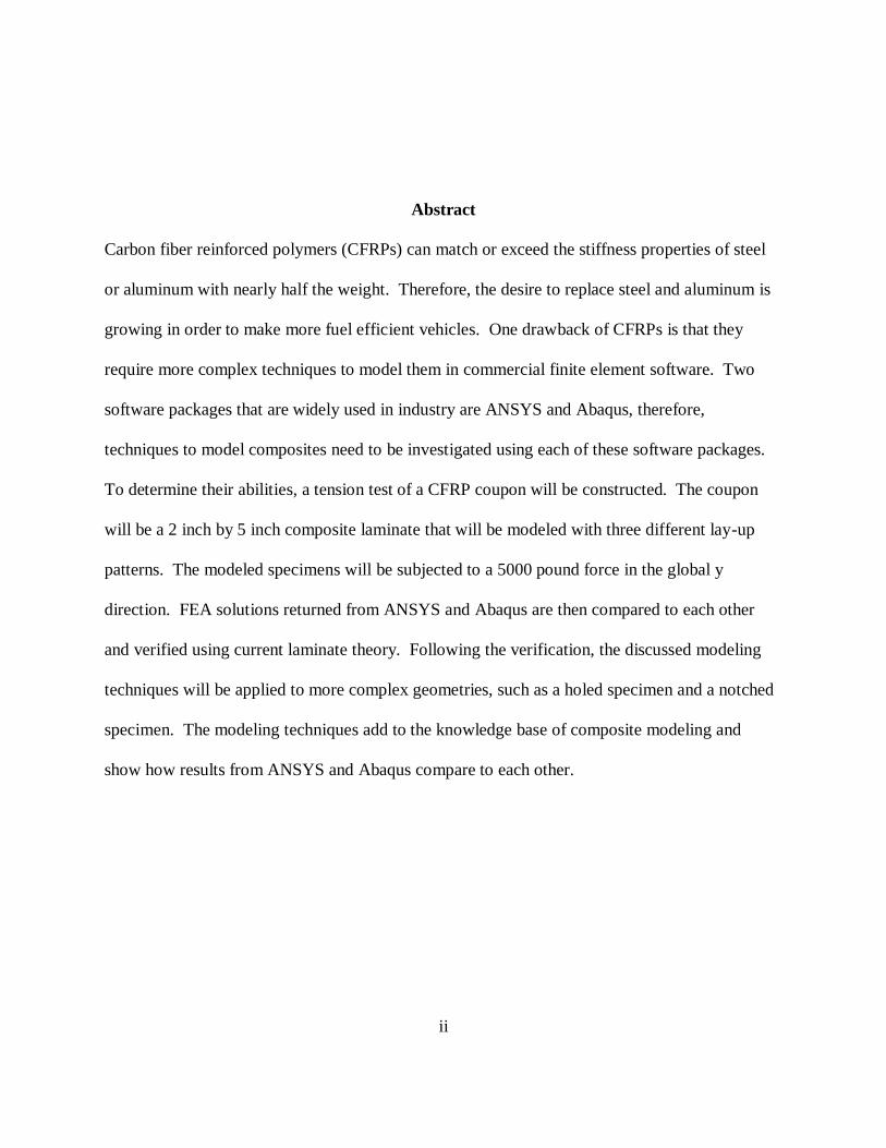
Abstract

Carbon fiber reinforced polymers (CFRPs) can match or exceed the stiffness properties of steel

or aluminum with nearly half the weight. Therefore, the desire to replace steel and aluminum is

growing in order to make more fuel efficient vehicles. One drawback of CFRPs is that they

require more complex techniques to model them in commercial finite element software. Two

software packages that are widely used in industry are ANSYS and Abaqus, therefore,

techniques to model composites need to be investigated using each of these software packages.

To determine their abilities, a tension test of a CFRP coupon will be constructed. The coupon

will be a 2 inch by 5 inch composite laminate that will be modeled with three different lay-up

patterns. The modeled specimens will be subjected to a 5000 pound force in the global y

direction. FEA solutions returned from ANSYS and Abaqus are then compared to each other

and verified using current laminate theory. Following the verification, the discussed modeling

techniques will be applied to more complex geometries, such as a holed specimen and a notched

specimen. The modeling techniques add to the knowledge base of composite modeling and

show how results from ANSYS and Abaqus compare to each other.

iii

Acknowledgements

I would like to thank Dr. Walter and Dr. Dupaix for the time that they have spent advising the

carbon fiber research team at The Ohio State University.

I would also like to thank Brooks Marquette and Hisham Sawan for being excellent team

members of the carbon fiber research team.

iv

Vita

2007 to present……………………...........Department of Mechanical and Aerospace Engineering

The Ohio State University.

Fields of Study

Major Field:

Bachelor of Science in Aeronautical and Astronautical Engineering

v

Table of Contents

Abstract ..................................................................................................................................... ii

Acknowledgements ................................................................................................................... iii

Vita ........................................................................................................................................... iv

Fields of Study .......................................................................................................................... iv

List of Figures .......................................................................................................................... vii

List of Tables ............................................................................................................................ ix

1. Introduction ........................................................................................................................... 10

1.1 Focus of Thesis ............................................................................................................... 13

1.2 Significance of Research ................................................................................................. 14

1.3 Overview of Thesis.......................................................................................................... 14

2. Laminate Analysis ................................................................................................................. 15

2.1 Theoretical laminate analysis ........................................................................................... 16

2.2 Laminate analysis using ANSYS ..................................................................................... 19

2.3 Laminate analysis using Abaqus ...................................................................................... 20

3 Modeling ................................................................................................................................ 22

3.1 Meshing and boundary conditions ................................................................................... 24

4 Simulation Results ................................................................................................................. 27

4.1 ANSYS Results ............................................................................................................... 27

vi

4.2 Abaqus Results ................................................................................................................ 28

4.3 Theoretical Results .......................................................................................................... 31

4.4 Results Summary ............................................................................................................. 33

5 Application of FEA to complex geometries ............................................................................ 38

5.1 Hole tension test .............................................................................................................. 38

5.2 Notch tension test ............................................................................................................ 42

6 Conclusions............................................................................................................................ 48

6.1 Contributions ................................................................................................................... 48

6.2 Additional Applications ................................................................................................... 48

6.3 Future Work .................................................................................................................... 49

6.4 Summary ......................................................................................................................... 49

Appendix A............................................................................................................................... 50

Appendix B ............................................................................................................................... 52

References ................................................................................................................................ 54

vii

List of Figures

Figure 1: Relative importance of material development through history (Staab, 1999) ............... 10

Figure 2: Envelopes comparing the Young’s modulus, E, vs. density, ρ, of various engineering

materials (Ashby, 2005) ............................................................................................................ 12

Figure 3: Envelopes comparing the strength, σf, vs. density, ρ, of various engineering materials

(Ashby, 2005) ........................................................................................................................... 12

Figure 4: Schematic of actual and modeled lamina (Staab, 1999) .............................................. 15

Figure 5: Sign convention of positive and negative fiber orientations (Staab, 1999) ................... 17

Figure 6: Unidirectional lay-up.................................................................................................. 22

Figure 7: Quasi-isotropic lay-up ................................................................................................ 23

Figure 8: Cross-ply lay-up ......................................................................................................... 23

Figure 9: Mesh and applied boundary conditions ....................................................................... 26

Figure 10: Stresses through the thickness of a unidirectional layup ............................................ 33

Figure 11: Stresses through the thickness of a quasi-isotropic layup .......................................... 35

Figure 12: Stresses through the thickness of a cross-ply layup ................................................... 35

Figure 13: Mesh used for the tension simulation of a holed specimen ........................................ 38

Figure 14: Stress in the y direction in layers 1 and 7 of a holed specimen in tension .................. 39



Figure 17: Stress in the y direction in layer 4 of a holed specimen in tension ............................. 42

Figure 18: Mesh used for the tension simulation of a notched specimen .................................... 43

Figure 19: Stress in the y direction in layers 1 and 7 of a notched specimen in tension .............. 44

viii



Figure 22: Stress in the y direction in layer 4 of a notched specimen in tension ......................... 47

ix

List of Tables

Table 1: Commercially available FEA software (Miracle & Donaldson, 2001) .......................... 13

Table 2: ANSYS elements that can be used for composite analysis (Anonymous_2, 2009) ........ 20

Table 3: ANSYS elements that can be used for composite analysis (Anonymous, 2008) ........... 21

Table 4: Elastic properties of each ply (Feraboli & Kedward, 2003) .......................................... 24

Table 5: ANSYS stress results throughout each ply of a unidirectional layup ............................ 27

Table 6: ANSYS stress results throughout each ply of a quasi-isotropic layup ........................... 28

Table 7: ANSYS stress results throughout each ply of a cross-ply layup.................................... 28

Table 8: Abaqus stress results throughout each ply of a quasi-isotropic layup (shown in the

principal directions) .................................................................................................................. 29

Table 9: Abaqus stress results throughout each ply of a quasi-isotropic layup ............................ 30

Table 10: Abaqus stress results throughout each ply of a unidirectional layup ........................... 31

Table 11: Abaqus stress results throughout each ply of a cross-ply layup................................... 31

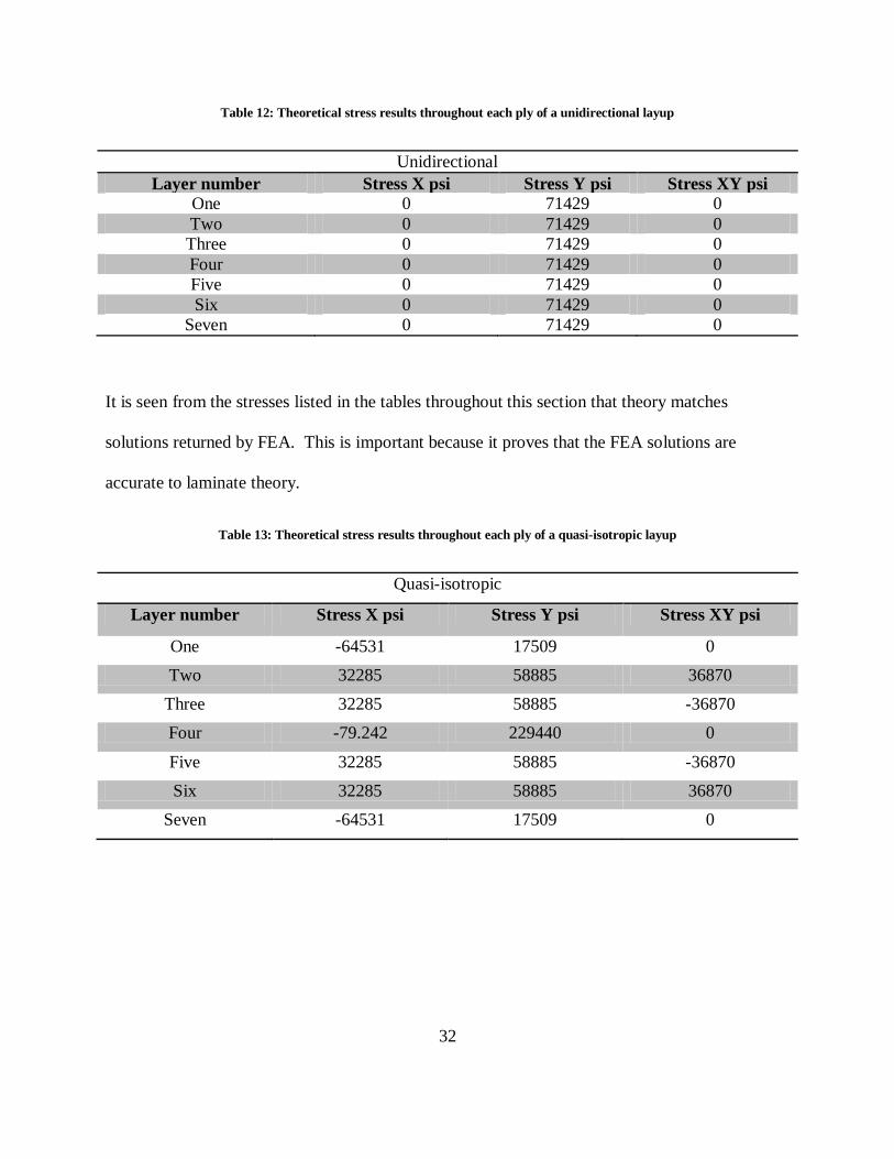
Table 12: Theoretical stress results throughout each ply of a unidirectional layup ..................... 32

Table 13: Theoretical stress results throughout each ply of a quasi-isotropic layup .................... 32

Table 14: Theoretical stress results throughout each ply of a cross-ply layup ............................. 33

Table 15: Average stress comparison ........................................................................................ 37

10

1. Introduction

The definition of a composite material is very flexible, but in the most general terms it is a

material that is composed of two or more distinct constituents. The use of composite materials in

engineering applications dates back to the ancient Egyptians and their use of straw in clay to

construct buildings (Swanson, 1997). In modern times composites have been used in civil

engineering applications, aerospace engineering applications, and many places in between. For

example, the automotive industry introduced large-scale use of composites with the Chevrolet

Corvette (Staab, 1999). The relative importance of composite development compared to other

engineering materials can be seen in Figure 1.

Figure 1: Relative importance of material development through history (Staab, 1999)

Automotive applications of composite materials, particularly carbon fiber reinforced polymers

(CFRPs), began with high performance vehicles. CFRPs were used to replace body panels, floor

panels, wheel housings, and hoods. This was done to reduce the weight of these vehicles in

11

order to increase their acceleration and speed on the race track. The high cost of CFRPs has

limited their use to high performance and racing vehicles. The increase in fuel costs and the

growing movement to reduce harmful emissions is pushing automobile companies to reduce the

weight of their vehicles in order to increase the fuel economy. A 10 percent reduction of vehicle

mass can increase a vehicles gas mileage by up to 7 percent (Unknown, 2008). Therefore, the

high strength-to-weight ratios of CFRPs is being sought to decrease the weight of the common

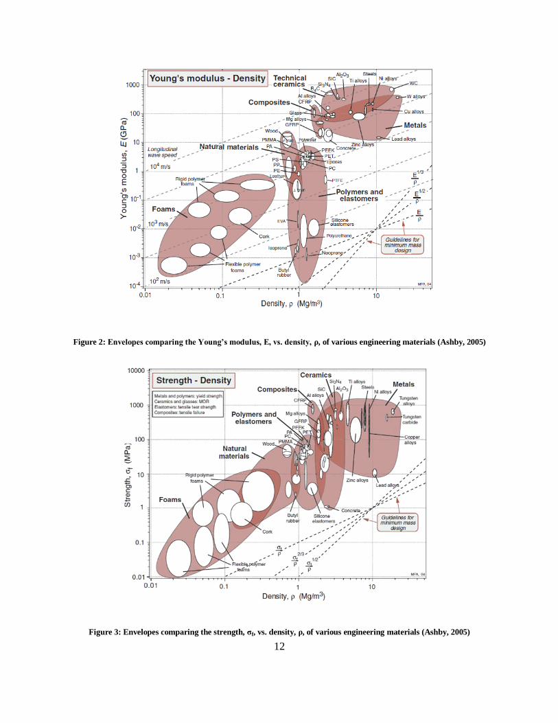
vehicle. A comparison of the strength-to-weight ratio properties of CFRPs to other materials can

be seen in Figure 2 and Figure 3.

Replacing car parts with CFRPs poses some problems to engineers. CFRP components are not

as simple to model as traditional engineering materials (steel, aluminum, etc.). First of all,

composite materials generally do not behave in an isotropic manner. Composite materials, such

as CFRPs, behave in an anisotropic or orthotropic manor. Anisotropic and orthotropic

mechanical behaviors are difficult to predict compared to isotropic behaviors. Therefore, finite

element analysis (FEA) packages must use more complex material models to predict these

behaviors. High performance composite components are made by bonding multiple plies of

unidirectional plies into a 3D laminate part.

12

Figure 2: Envelopes comparing the Young’s modulus, E, vs. density, ρ, of various engineering materials (Ashby, 2005)

Figure 3: Envelopes comparing the strength, σf, vs. density, ρ, of various engineering materials (Ashby, 2005)

13

1.1 Focus of Thesis

The finite element method (FEM) is used to predict multiple types of static and dynamic

structural responses. For example, companies in the automotive industry use it to predict, stress,

strain, deformations, and failure of many different types of components. FEA reduces the need

for costly experiments and allows engineers to optimize parts before they are built and

implemented. There are many software packages available to industries that use FEA. A list of

some of these commercial packages can be seen in Table 1.

Table 1: Commercially available FEA software (Miracle & Donaldson, 2001)

The focus of the thesis is to compare the composite analysis abilities of ANSYS and Abaqus.

The comparison will be completed by modeling composite laminates of different orientations.

Out of the packages listed above, ANSYS and Abaqus were selected due to their availability at

The Ohio State University and their wide usage in industry and research.

14

1.2 Significance of Research

Composite materials have very different structural responses than traditional materials. This is

mainly due to their anisotropic and orthotropic elastic behavior. Therefore, for an engineer to

properly design a composite he/she must understand how to construct a model in FEA software.

A fundamental understanding of composite modeling will allow engineers to design car parts

that match or exceed the performance of steel or aluminum parts. The stronger and lighter parts

will lead to safer more fuel efficient vehicles. This research will provide insight on the

differences between ANSYS and Abaqus along with a fundamental understanding of creating

composite models.

1.3 Overview of Thesis

This thesis has 5 chapters. Chapter 2 consists of a discussion on the theory behind lamina

analysis. The theoretical discussion will focus on the theory used to construct a MATLAB code

used to verify the FEA results. Chapter 3 will discuss the setup of the FEA models in ANSYS

and Abaqus. It will discuss the tests that were modeled, the material models used, element types,

and the unique attributes of each FEA package. The results from the simulations and theoretical

calculations will be compared to each other in Chapter 4. ANSYS will then be used to simulate

a holed and notched tension specimen in chapter 5. Then in the final chapter conclusions will be

drawn, contributions will be discussed, applications will be described, and future work will be

proposed. The thesis will also be briefly summarized in order to reiterate the big picture of the

research.

15

2. Laminate Analysis

Laminated composite materials are much more difficult to analyze compared to traditional

materials. This is due to the fact that the mechanical response of a composite material is

dependent on the direction of loading and they tend to react in an anisotropic or orthotropic

manner. In order to analyze the mechanical response of a laminate, the behavior of each

individual ply must be predicted (Staab, 1999). To do so, assumptions were made and theories

were derived.

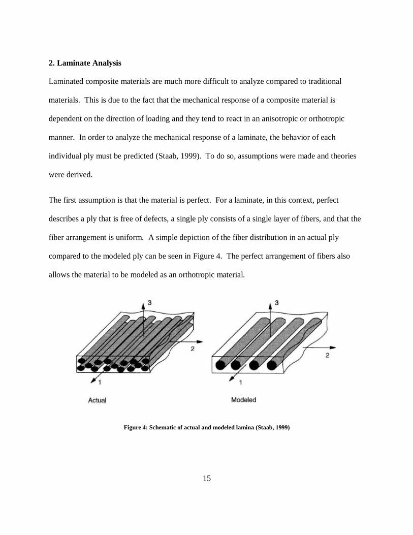
The first assumption is that the material is perfect. For a laminate, in this context, perfect

describes a ply that is free of defects, a single ply consists of a single layer of fibers, and that the

fiber arrangement is uniform. A simple depiction of the fiber distribution in an actual ply

compared to the modeled ply can be seen in Figure 4. The perfect arrangement of fibers also

allows the material to be modeled as an orthotropic material.

Figure 4: Schematic of actual and modeled lamina (Staab, 1999)

16

Laminate theories were used in order to validate tension tests simulated using FEA. These

theories calculate the stress across the thickness of each ply of the laminate. The theory will be

discussed in the following text.

2.1 Theoretical laminate analysis

For the discussion subscripts 1, 2, and 3 will represent principal fiber direction, in-plane

direction perpendicular to the fibers, and out-of-plane direction perpendicular to the fibers.

These numbers also represent the principal axes of the orthotropic material behavior. These axes

can also be seen in Figure 4.

For the analysis throughout this section the lamina will be analyzed using plane stress conditions.

Assuming plane stress conditions reduces the level of complexity of the analysis because the

model is reduced from three dimensional to two dimensional. Therefore, this analysis is only

concerned with the material properties in principal directions 1 and 2. To predict the axial stress

in a lamina , , , and must be provided for the material in question. The number of

plies, their thickness, width, and orientation must also be provided.

To initiate the stress calculations, the provided material properties can be used to calculate .

This Poisson’s ratio was calculated using the following equation (Staab, 1999).

The provided moduli and Poisson’s ratios can be used to construct a stiffness matrix. The

stiffness matrix for plane stress conditions can be seen in the matrix below (Staab, 1999).

17

[ ] [

]

In this matrix the individual terms are

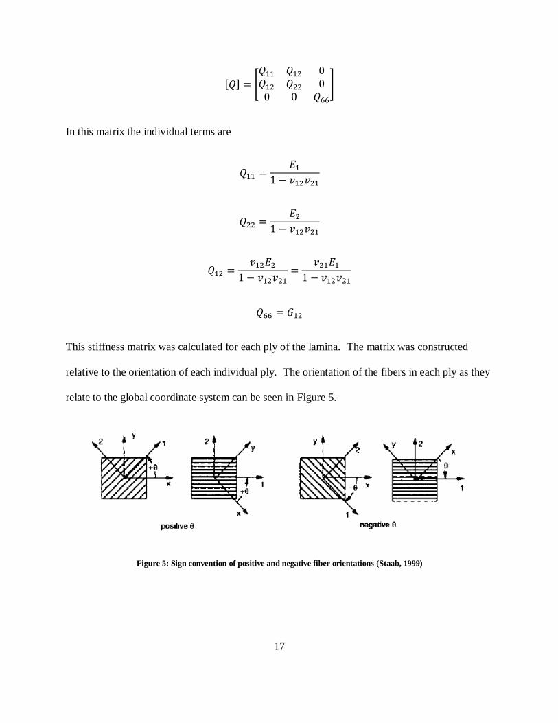
This stiffness matrix was calculated for each ply of the lamina. The matrix was constructed

relative to the orientation of each individual ply. The orientation of the fibers in each ply as they

relate to the global coordinate system can be seen in Figure 5.

Figure 5: Sign convention of positive and negative fiber orientations (Staab, 1999)

18

The stiffness matrix for each of the plies has to be transformed into the global coordinate system

in order to obtain the stresses in the global directions. This transformation will formulate a new

stiffness matrix, seen below (Staab, 1999).

[ ] [

]

In the converted stiffness matrix the individual terms are ( )

( )

( ) (

)

( ) ( )

( )

( ) ( )

( ) (

)

The [ ] matrices for each of the different plies are then added together. This summed matrix

will be represented by [ ] . The total matrix can be used to predict the strain that is caused

by an applied tensile stress. This calculation can be seen in the equation below.

[

] [ ]

[

]

19

The stress throughout the lamina can then be predicted using the following relation (Staab,

1999).

{

} [

] {

}

2.2 Laminate analysis using ANSYS

Within ANSYS there are many different elements that can be used to model composite lay ups.

The element types used by ANSYS are referred to as finite strain shell elements, 3D layered

structural solid shell elements, and 3D layered structural solid elements. There are a variety of

specific elements associated with each element type. Specific element selection depends upon

application and the type of results that must be calculated (Anonymous_2, 2009). Different

finite strain shell elements can be chosen depending on the number of composite layers, the

thickness of each layer, and the expected magnitude of the displacements/rotations of the model.

Selection of 3D layered structural solid elements is based upon the geometry of the structure

being modeled. Structures with through the thickness discontinuities or that have a wide range

of shell thicknesses within the part should be modeled using 3D layered structural shell elements.

The most complex of the previously stated element types is the 3D layered structural element.

This element type should be selected to model exotic 3D geometries. This element type should

also be selected if information about plasticity, hyperelasticity, stress stiffening, creep, large

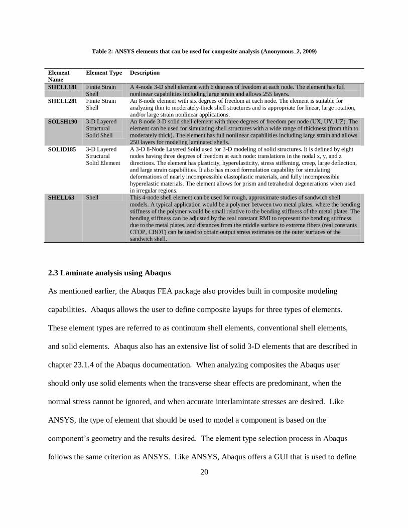
deflections, and large strains is desired. A list of specific elements and their elements types can

be seen in Table 2.

20

Table 2: ANSYS elements that can be used for composite analysis (Anonymous_2, 2009)

Element

Name

Element Type Description

SHELL181 Finite Strain

Shell

A 4-node 3-D shell element with 6 degrees of freedom at each node. The element has full

nonlinear capabilities including large strain and allows 255 layers.

SHELL281 Finite Strain Shell

An 8-node element with six degrees of freedom at each node. The element is suitable for analyzing thin to moderately-thick shell structures and is appropriate for linear, large rotation, and/or large strain nonlinear applications.

SOLSH190 3-D Layered Structural Solid Shell

An 8-node 3-D solid shell element with three degrees of freedom per node (UX, UY, UZ). The element can be used for simulating shell structures with a wide range of thickness (from thin to moderately thick). The element has full nonlinear capabilities including large strain and allows 250 layers for modeling laminated shells.

SOLID185 3-D Layered Structural Solid Element

A 3-D 8-Node Layered Solid used for 3-D modeling of solid structures. It is defined by eight nodes having three degrees of freedom at each node: translations in the nodal x, y, and z directions. The element has plasticity, hyperelasticity, stress stiffening, creep, large deflection, and large strain capabilities. It also has mixed formulation capability for simulating deformations of nearly incompressible elastoplastic materials, and fully incompressible hyperelastic materials. The element allows for prism and tetrahedral degenerations when used in irregular regions.

SHELL63 Shell This 4-node shell element can be used for rough, approximate studies of sandwich shell

models. A typical application would be a polymer between two metal plates, where the bending stiffness of the polymer would be small relative to the bending stiffness of the metal plates. The bending stiffness can be adjusted by the real constant RMI to represent the bending stiffness due to the metal plates, and distances from the middle surface to extreme fibers (real constants CTOP, CBOT) can be used to obtain output stress estimates on the outer surfaces of the sandwich shell.

2.3 Laminate analysis using Abaqus

As mentioned earlier, the Abaqus FEA package also provides built in composite modeling

capabilities. Abaqus allows the user to define composite layups for three types of elements.

These element types are referred to as continuum shell elements, conventional shell elements,

and solid elements. Abaqus also has an extensive list of solid 3-D elements that are described in

chapter 23.1.4 of the Abaqus documentation. When analyzing composites the Abaqus user

should only use solid elements when the transverse shear effects are predominant, when the

normal stress cannot be ignored, and when accurate interlamintate stresses are desired. Like

ANSYS, the type of element that should be used to model a component is based on the

component’s geometry and the results desired. The element type selection process in Abaqus

follows the same criterion as ANSYS. Like ANSYS, Abaqus offers a GUI that is used to define

21

the properties of a layered composite structure. This GUI is referred to as the composite layup

editor. The composite layup editor provides a table that the user can use to define the plies in the

layup (Anonymous, 2008). This table can be used to assign a name, material, thickness, and

orientation to each ply. The ply table also provides several options that make it easier for the

user to create a layered composite containing many plies. These options include; the ability to

move or copy selected plies up or down in the table, suppress or delete plies, create patterns with

a group of selected plies, and read ply data from or write data to an ASCII file. The ability to

suppress plies allows the user to easily experiment with different configurations of plies in the

composite layup and see the effect on the results of an analysis of a model (Anonymous, 2008).

A list the element types and specific elements names used by Abaqus to analyze composites can

be seen in Table 3.

Table 3: ANSYS elements that can be used for composite analysis (Anonymous, 2008)

Element

Name

Element Type Description

STRI3(S)

Conventional Shell 3-node triangular facet thin shell

S3 Conventional Shell 3-node triangular general-purpose shell, finite membrane strains (identical to element S3R)

S3R Conventional Shell 3-node triangular general-purpose shell, finite membrane strains (identical to element S3)

S3RS(E)

Conventional Shell 3-node triangular shell, small membrane strains

STRI65(S)

Conventional Shell 6-node triangular thin shell, using five degrees of freedom per node

S4 Conventional Shell 4-node doubly curved general-purpose shell, finite membrane strains

S4R Conventional Shell 4-node doubly curved general-purpose shell, reduced integration with hourglass control, finite membrane strains

S4RS(E)

Conventional Shell 4-node, reduced integration, doubly curved shell with hourglass control, small membrane strains

S4RSW(E)

Conventional Shell 4-node, reduced integration, doubly curved shell with hourglass control, small membrane

strains, warping considered in small-strain formulation

S4R5(S)

Conventional Shell 4-node doubly curved thin shell, reduced integration with hourglass control, using five degrees of freedom per node

S8R(S)

Conventional Shell 8-node doubly curved thick shell, reduced integration

S8R5(S)

Conventional Shell 8-node doubly curved thin shell, reduced integration, using five degrees of freedom per node

S9R5(S)

Conventional Shell 9-node doubly curved thin shell, reduced integration, using five degrees of freedom per node

SC6R Continuum Shell 6-node triangular in-plane continuum shell wedge, general-purpose, finite membrane

strains

SC8R Continuum Shell 8-node hexahedron, general-purpose, finite membrane strains

22

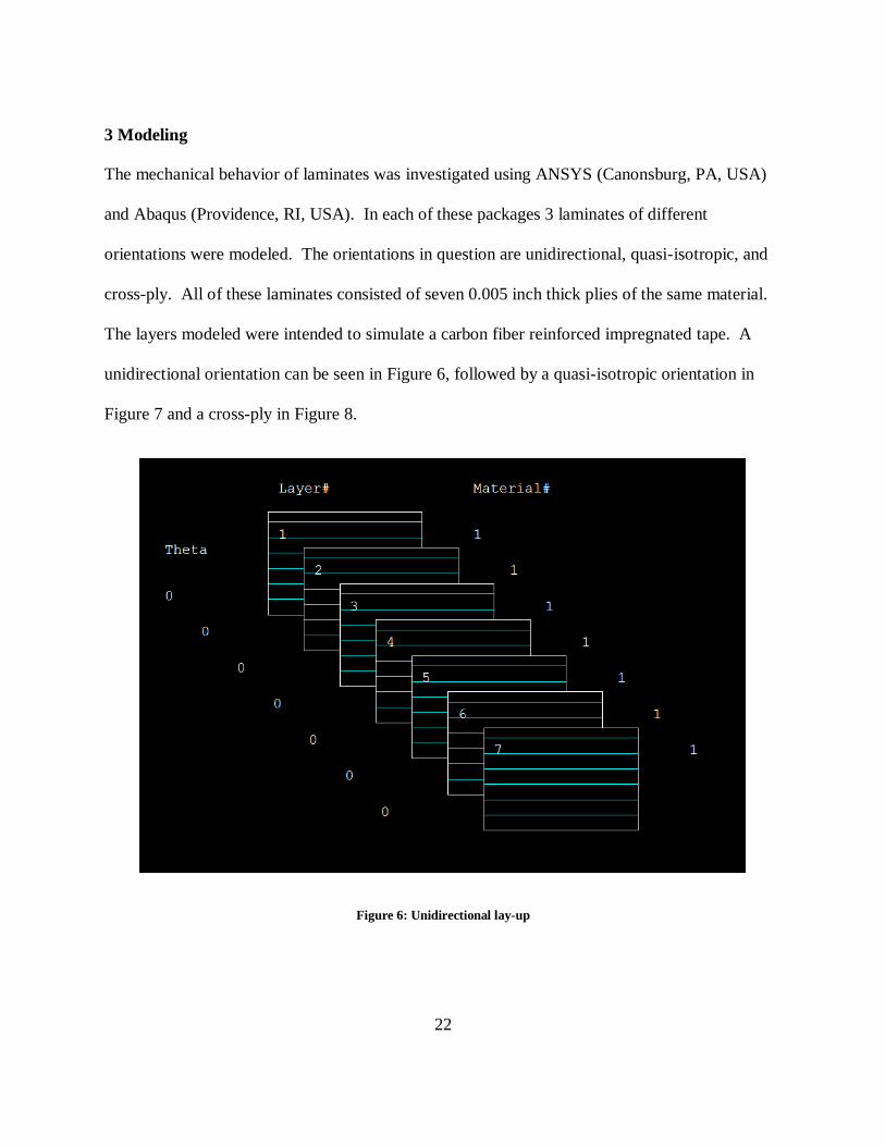
3 Modeling

The mechanical behavior of laminates was investigated using ANSYS (Canonsburg, PA, USA)

and Abaqus (Providence, RI, USA). In each of these packages 3 laminates of different

orientations were modeled. The orientations in question are unidirectional, quasi-isotropic, and

cross-ply. All of these laminates consisted of seven 0.005 inch thick plies of the same material.

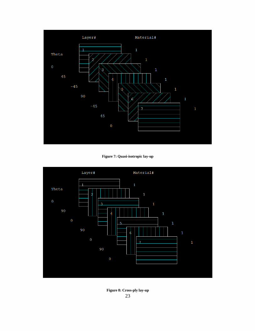
The layers modeled were intended to simulate a carbon fiber reinforced impregnated tape. A

unidirectional orientation can be seen in Figure 6, followed by a quasi-isotropic orientation in

Figure 7 and a cross-ply in Figure 8.

Figure 6: Unidirectional lay-up

23

Figure 7: Quasi-isotropic lay-up

Figure 8: Cross-ply lay-up

24

Material properties for each ply were prescribed using the properties in Table 4. This type of

carbon-fiber composite has a modulus that is roughly 12 times stiffer in the direction of the fibers

than transverse to the fibers. Also, the anisotropy effects are less important in shear/Poisson’s

ratio. These two phenomena are due to the fact that the fibers are much stiffer than the

surrounding matrix.

Table 4: Elastic properties of each ply (Feraboli & Kedward, 2003)

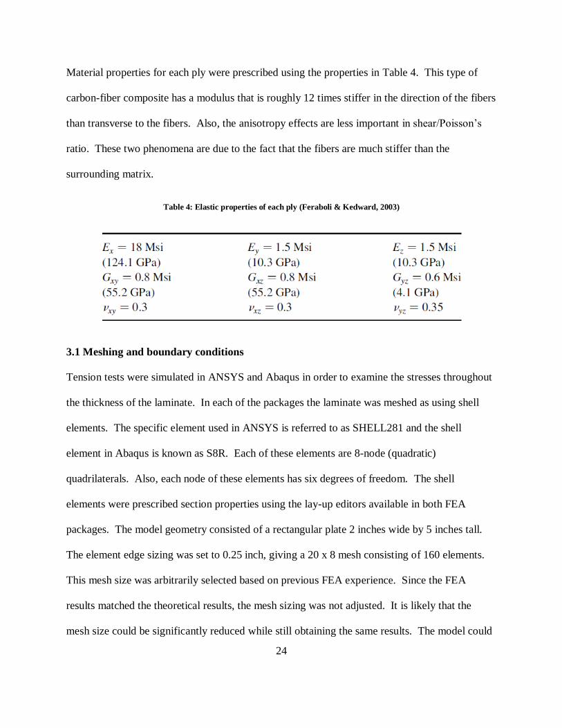
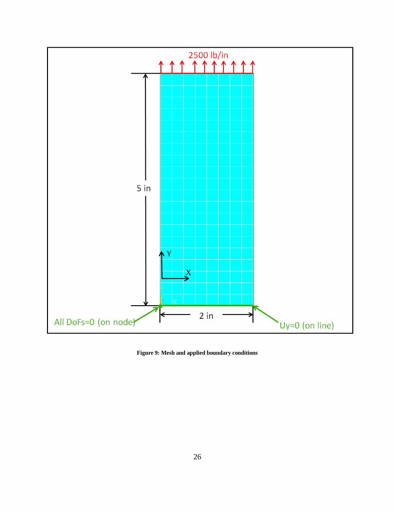
3.1 Meshing and boundary conditions

Tension tests were simulated in ANSYS and Abaqus in order to examine the stresses throughout

the thickness of the laminate. In each of the packages the laminate was meshed as using shell

elements. The specific element used in ANSYS is referred to as SHELL281 and the shell

element in Abaqus is known as S8R. Each of these elements are 8-node (quadratic)

quadrilaterals. Also, each node of these elements has six degrees of freedom. The shell

elements were prescribed section properties using the lay-up editors available in both FEA

packages. The model geometry consisted of a rectangular plate 2 inches wide by 5 inches tall.

The element edge sizing was set to 0.25 inch, giving a 20 x 8 mesh consisting of 160 elements.

This mesh size was arbitrarily selected based on previous FEA experience. Since the FEA

results matched the theoretical results, the mesh sizing was not adjusted. It is likely that the

mesh size could be significantly reduced while still obtaining the same results. The model could

25

have also been simplified by applying quarter symmetry. Since computational cost wasn’t an

issue for this test the selected mesh size wasn’t adjusted and the entire tension specimen was

modeled. For more complex models, where computational cost maybe an issue, it would be

useful to apply any simplifications that can be justified.

For the simulation the bottom edge of the test coupon was constrained and a force was applied to

the top edge. The line on the bottom of the shell was constrained in the y-direction. Also, to

allow for Poisson’s effects and to prevent rigid body motion, the node at the bottom corner was

constrained in all degrees of freedom. The force was prescribed to be distributed evenly across

the top edge of the shell. To simulate a total force of 5000 pounds, an edge pressure of 2500

pounds per inch had to be prescribed. This model is an idealization of a tension test. In reality

the grips used to hold the tension coupon would apply more of a constraint in the x direction,

which would cause the stress near the edge of the part to be non-uniform. These effects can be

accounted for by making the tension specimen taller. This is justified by Saint-Venant’s

principle. Also, since the constraints in the model are perfect, the height of the specimen doesn’t

affect the FEA solution. An illustration of the previously described boundary conditions and

forces can be seen in Figure 9.

26

Figure 9: Mesh and applied boundary conditions

Y

X

27

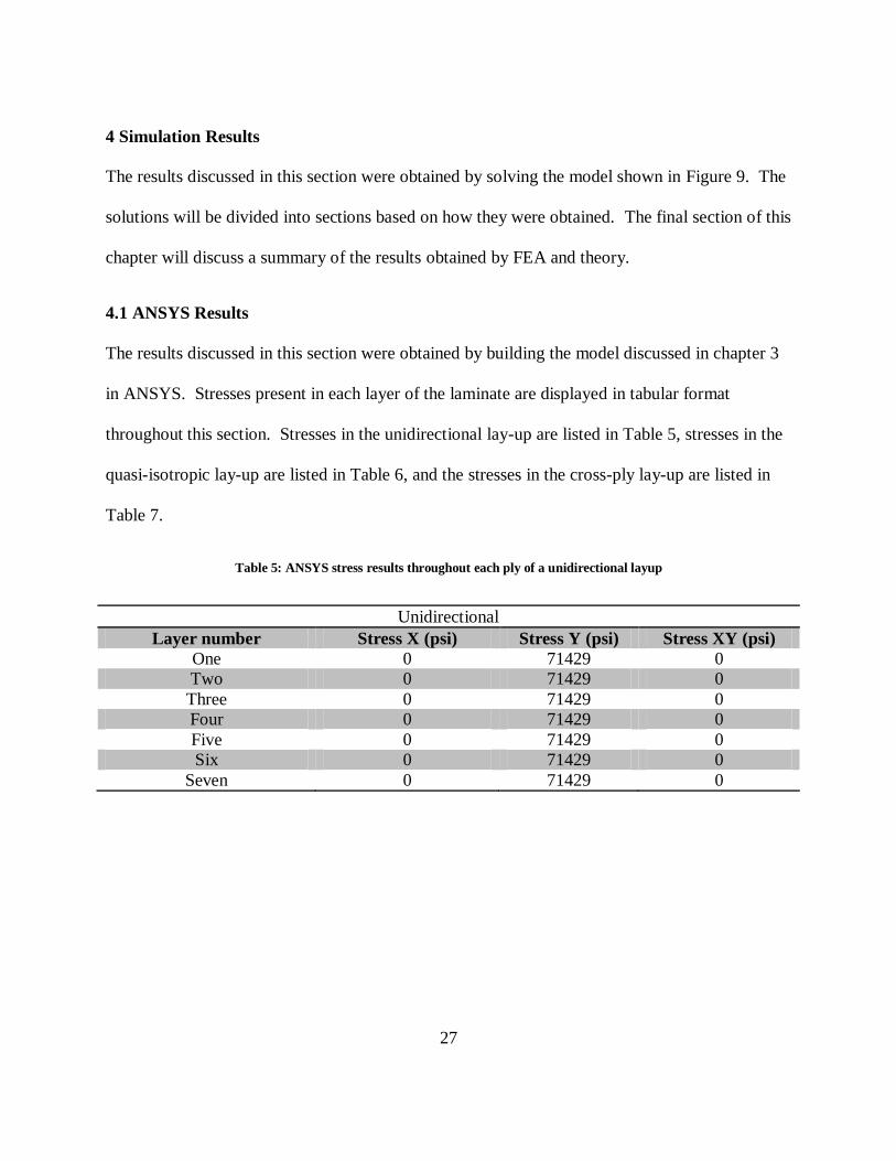
4 Simulation Results

The results discussed in this section were obtained by solving the model shown in Figure 9. The

solutions will be divided into sections based on how they were obtained. The final section of this

chapter will discuss a summary of the results obtained by FEA and theory.

4.1 ANSYS Results

The results discussed in this section were obtained by building the model discussed in chapter 3

in ANSYS. Stresses present in each layer of the laminate are displayed in tabular format

throughout this section. Stresses in the unidirectional lay-up are listed in Table 5, stresses in the

quasi-isotropic lay-up are listed in Table 6, and the stresses in the cross-ply lay-up are listed in

Table 7.

Table 5: ANSYS stress results throughout each ply of a unidirectional layup

Unidirectional

Layer number Stress X (psi) Stress Y (psi) Stress XY (psi)

One 0 71429 0

Two 0 71429 0

Three 0 71429 0

Four 0 71429 0

Five 0 71429 0

Six 0 71429 0

Seven 0 71429 0

28

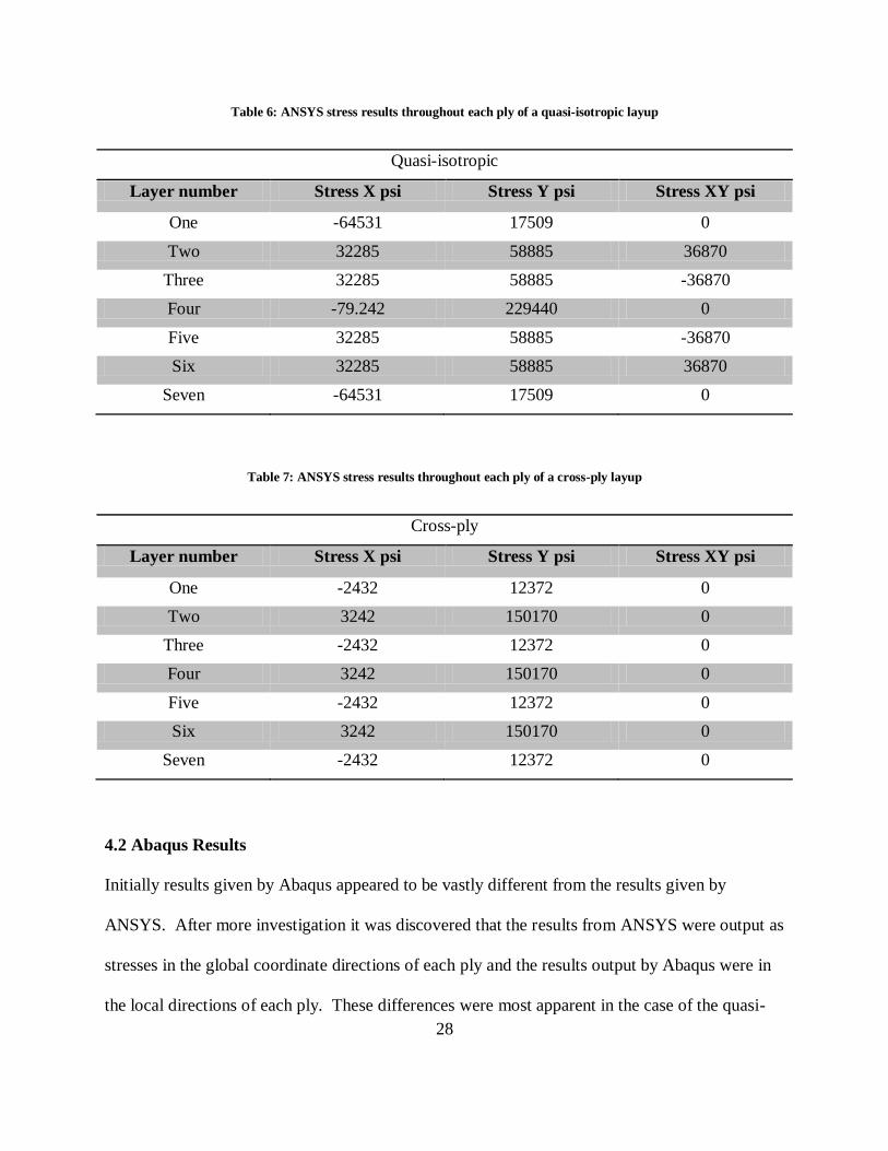
Table 6: ANSYS stress results throughout each ply of a quasi-isotropic layup

Quasi-isotropic

Layer number Stress X psi Stress Y psi Stress XY psi

One -64531 17509 0

Two 32285 58885 36870

Three 32285 58885 -36870

Four -79.242 229440 0

Five 32285 58885 -36870

Six 32285 58885 36870

Seven -64531 17509 0

Table 7: ANSYS stress results throughout each ply of a cross-ply layup

Cross-ply


One -2432 12372 0

Two 3242 150170 0

Three -2432 12372 0

Four 3242 150170 0

Five -2432 12372 0

Six 3242 150170 0

Seven -2432 12372 0

4.2 Abaqus Results

Initially results given by Abaqus appeared to be vastly different from the results given by

ANSYS. After more investigation it was discovered that the results from ANSYS were output as

stresses in the global coordinate directions of each ply and the results output by Abaqus were in

the local directions of each ply. These differences were most apparent in the case of the quasi-

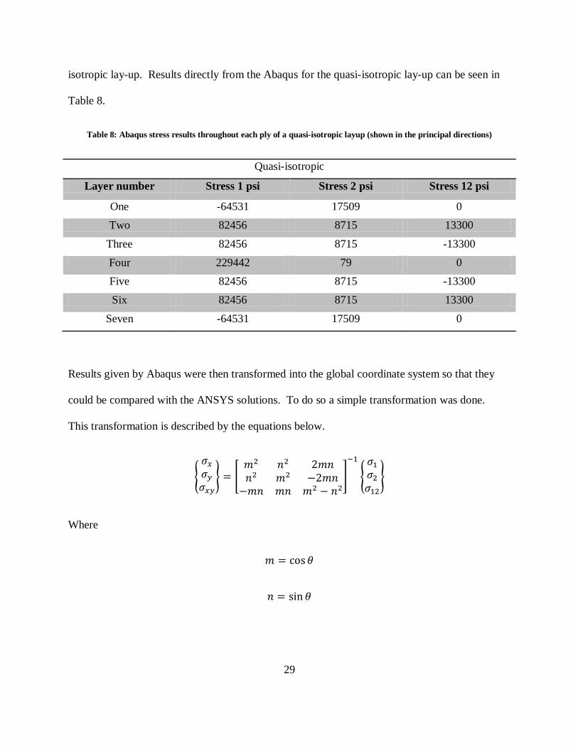
29

isotropic lay-up. Results directly from the Abaqus for the quasi-isotropic lay-up can be seen in

Table 8.

Table 8: Abaqus stress results throughout each ply of a quasi-isotropic layup (shown in the principal directions)

Quasi-isotropic

Layer number Stress 1 psi Stress 2 psi Stress 12 psi

One -64531 17509 0

Two 82456 8715 13300

Three 82456 8715 -13300

Four 229442 79 0

Five 82456 8715 -13300

Six 82456 8715 13300

Seven -64531 17509 0

Results given by Abaqus were then transformed into the global coordinate system so that they

could be compared with the ANSYS solutions. To do so a simple transformation was done.

This transformation is described by the equations below.

{

} [

]

{

}

Where

30

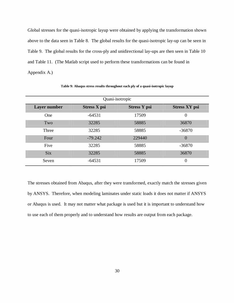
Global stresses for the quasi-isotropic layup were obtained by applying the transformation shown

above to the data seen in Table 8. The global results for the quasi-isotropic lay-up can be seen in

Table 9. The global results for the cross-ply and unidirectional lay-ups are then seen in Table 10

and Table 11. (The Matlab script used to perform these transformations can be found in

Appendix A.)

Table 9: Abaqus stress results throughout each ply of a quasi-isotropic layup

Quasi-isotropic


One -64531 17509 0

Two 32285 58885 36870

Three 32285 58885 -36870

Four -79.242 229440 0

Five 32285 58885 -36870

Six 32285 58885 36870

Seven -64531 17509 0

The stresses obtained from Abaqus, after they were transformed, exactly match the stresses given

by ANSYS. Therefore, when modeling laminates under static loads it does not matter if ANSYS

or Abaqus is used. It may not matter what package is used but it is important to understand how

to use each of them properly and to understand how results are output from each package.

31

Table 10: Abaqus stress results throughout each ply of a unidirectional layup

Unidirectional

Layer number Stress X psi Stress Y psi Stress XY psi One 0 71429 0

Two 0 71429 0

Three 0 71429 0

Four 0 71429 0

Five 0 71429 0

Six 0 71429 0

Seven 0 71429 0 Table 11: Abaqus stress results throughout each ply of a cross-ply layup

Cross-ply


One -2432 12372 0

Two 3242 150170 0

Three -2432 12372 0

Four 3242 150170 0

Five -2432 12372 0

Six 3242 150170 0

Seven -2432 12372 0

4.3 Theoretical Results

To verify the FEA solutions the theory discussed in chapter 2 was applied to the geometry and

loading conditions shown in Figure 9. The results for the three different lay-ups of interest are

listed in Table 12, Table 13, and Table 14. (The Matlab script used to calculate the theoretical

results was provided by Brooks Marquette and can be found in Appendix B.)

32

Table 12: Theoretical stress results throughout each ply of a unidirectional layup

Unidirectional

Layer number Stress X psi Stress Y psi Stress XY psi One 0 71429 0

Two 0 71429 0

Three 0 71429 0

Four 0 71429 0

Five 0 71429 0

Six 0 71429 0

Seven 0 71429 0

It is seen from the stresses listed in the tables throughout this section that theory matches

solutions returned by FEA. This is important because it proves that the FEA solutions are

accurate to laminate theory.

Table 13: Theoretical stress results throughout each ply of a quasi-isotropic layup

Quasi-isotropic


One -64531 17509 0

Two 32285 58885 36870

Three 32285 58885 -36870

Four -79.242 229440 0

Five 32285 58885 -36870

Six 32285 58885 36870

Seven -64531 17509 0

33

Table 14: Theoretical stress results throughout each ply of a cross-ply layup

Cross-ply


One -2432 12372 0

Two 3242 150170 0

Three -2432 12372 0

Four 3242 150170 0

Five -2432 12372 0

Six 3242 150170 0

Seven -2432 12372 0

4.4 Results Summary

The results shown throughout the previous three sections of this chapter were reduced to three

plots of the stresses through the thickness of the laminate. A plot of the stress through a

unidirectional layup is seen in Figure 10.

Figure 10: Stresses through the thickness of a unidirectional layup

-0.02 -0.015 -0.01 -0.005 0 0.005 0.01 0.015 0.020

1

2

3

4

5

6

7

8x 10

4 LAMINATE STRESS

z(in)

Str

ess(p

si)

STRESSX

STRESSY

STRESSXY

34

Figure 10 shows that the only stress present throughout the unidirectional lay-up is in the y

direction. Stress only exists in the y direction because each layer is oriented perpendicular to the

direction of loading. This would also be true if the all of the layers were oriented parallel to the

direction of loading. For the tension tests discussed in this document, the only time that stress

will simultaneously be present in the x, y, and xy directions will be in the multi-directional

layups. The plot of the stress through the thickness of a quasi-isotropic lay-up can be seen in

Figure 11 and for a cross-ply this plot is seen in Figure 12.

Shear and lateral stresses will never exist in any type of unidirectional layup where the loading is

parallel or perpendicular to the fiber directions. This is seen mathematically in the [ ] matrix. If

the fibers are oriented at 0 or 90 degrees the shear terms, and , go to zero. Any other

case where the fibers aren’t parallel or perpendicular to the loading direction the shear terms

wouldn’t be zero; therefore, there will be shear stresses through the part.

The stresses throughout the thickness of a quasi-isotropic lay-up are much more interesting than

the stresses through a unidirectional lay-up. As is seen in Figure 11, the stress in the y direction

of the center ply is much higher than any of the other plies. This is expected because the center

ply is oriented with the fibers parallel to the direction of loading. Since strains are considered to

be equal in every ply and the center ply is has the highest stiffness in the direction of loading, the

center ply should therefore have the highest stress. Figure 11 also shows that the stresses in ply

1 are equal to stresses in ply 7, stresses in ply 2 are equal to stresses in ply 6, and stresses in ply 3

are equal to stresses in ply 5. This symmetry condition can be applied to simplify each of the

models. The same symmetry condition is shown by the unidirectional and cross-ply lay-ups.

35

Figure 11: Stresses through the thickness of a quasi-isotropic layup

Figure 12: Stresses through the thickness of a cross-ply layup

-0.02 -0.015 -0.01 -0.005 0 0.005 0.01 0.015 0.02-1

-0.5

0

0.5

1

1.5

2

2.5x 10

5 LAMINATE STRESS

z(in)

Str

ess(p

si)

STRESSX

STRESSY

STRESSXY

-0.02 -0.015 -0.01 -0.005 0 0.005 0.01 0.015 0.02-2

0

2

4

6

8

10

12

14

16x 10

4 LAMINATE STRESS

z(in)

Str

ess(p

si)

STRESSX

STRESSY

STRESSXY

36

The stresses seen throughout the thickness of the cross-ply lay-up are also expected. Since the

fiber orientations alternate back and forth between being perpendicular and parallel with the

direction of loading, it is expected the stress in the y direction should go from low to high

because of the large variation of the stiffness in the direction of loading. It is also seen that the

stress in the xy direction is also zero. This is because the direction of loading is always parallel

to a principal direction of a respective ply.

The average stress throughout the thickness of a respective lay-up can also be used to further

verify the results. The following equation can be used to check the average stress.

Where, in the case of this simulation

Therefore,

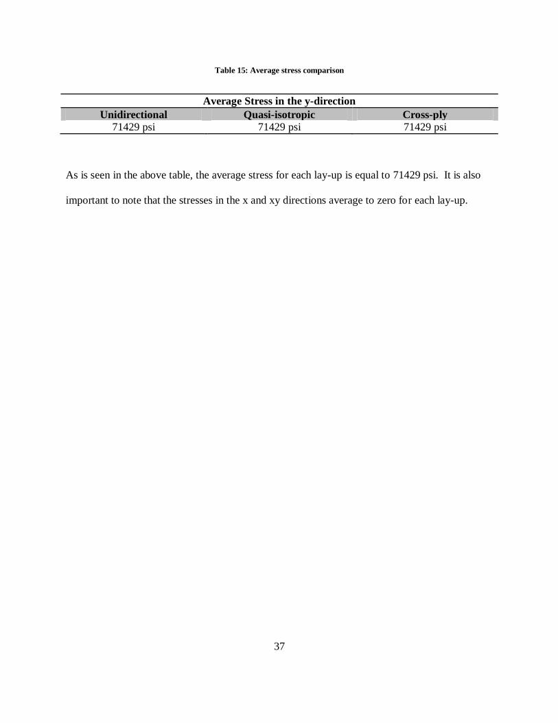
The stress value shown is equal to the average stress in the y direction throughout each

respective laminate. The average stresses in the y-direction for each lay-up are shown in Table

15

37

Table 15: Average stress comparison

Average Stress in the y-direction

Unidirectional Quasi-isotropic Cross-ply

71429 psi 71429 psi 71429 psi

As is seen in the above table, the average stress for each lay-up is equal to 71429 psi. It is also

important to note that the stresses in the x and xy directions average to zero for each lay-up.

38

5 Application of FEA to complex geometries

Since the finite element code has been proved to be accurate to theory it is plausible to begin

solving tension tests of more complex geometries. Two more complex geometries are shown

throughout this chapter; they are a holed specimen and a notched specimen.

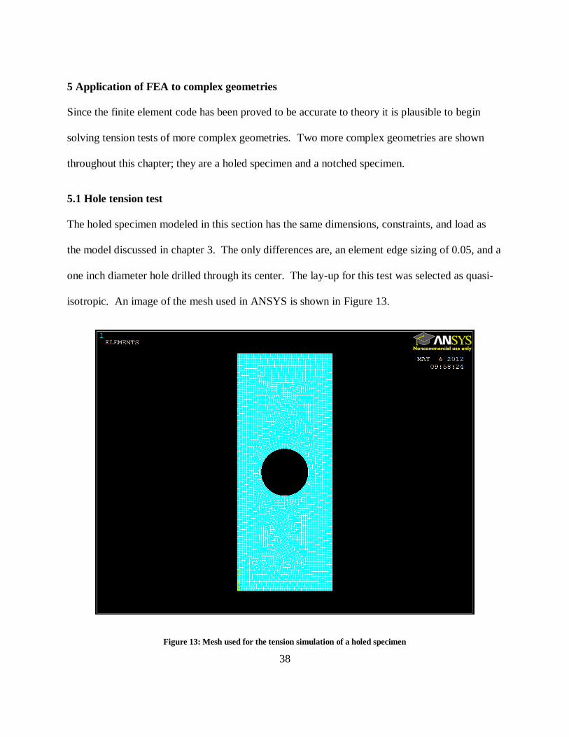
5.1 Hole tension test

The holed specimen modeled in this section has the same dimensions, constraints, and load as

the model discussed in chapter 3. The only differences are, an element edge sizing of 0.05, and a

one inch diameter hole drilled through its center. The lay-up for this test was selected as quasi-

isotropic. An image of the mesh used in ANSYS is shown in Figure 13.

Figure 13: Mesh used for the tension simulation of a holed specimen

39

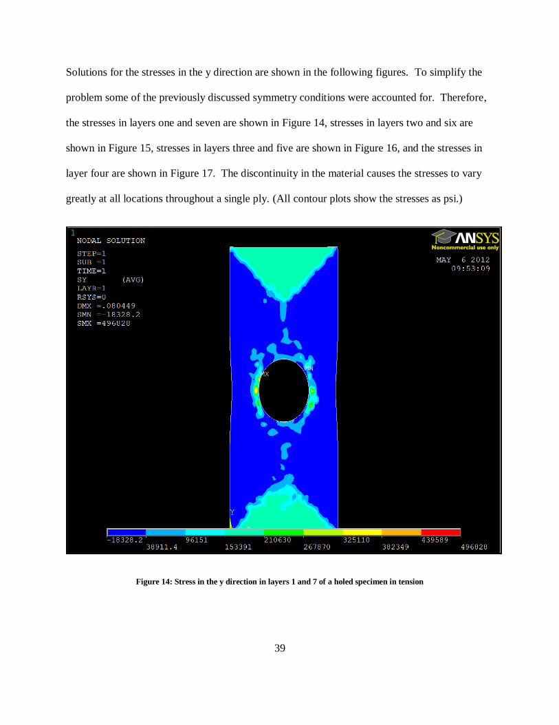
Solutions for the stresses in the y direction are shown in the following figures. To simplify the

problem some of the previously discussed symmetry conditions were accounted for. Therefore,

the stresses in layers one and seven are shown in Figure 14, stresses in layers two and six are

shown in Figure 15, stresses in layers three and five are shown in Figure 16, and the stresses in

layer four are shown in Figure 17. The discontinuity in the material causes the stresses to vary

greatly at all locations throughout a single ply. (All contour plots show the stresses as psi.)

Figure 14: Stress in the y direction in layers 1 and 7 of a holed specimen in tension

40


The contour plots shown for each layer of the holed specimen display some peculiar behaviors.

In the unidirectional ply shown in Figure 14 it is seen that there are triangular shaped regions

near the constrained and loaded edges. These triangular regions contain an average stress

between 150 ksi and 200 ksi. Outside of these regions the stress then drops to -18 ksi until it

begins to increase again in the presence of the hole. Figure 14 can then be compared to Figure

17, which is the 90 degree ply. The 90 degree ply also shows triangular contours at the loaded

and constrained edges. Only in these triangles the stress is lower than the regions directly

outside of the triangle. The contour shapes in Figure 14 and Figure 17 show similar trends, but

41

the contours are inverted as far as their relative magnitudes. This should be expected since the

first ply is loaded perpendicular to the fiber direction and the fourth ply is loaded parallel to the

fiber direction. The material has the lowest stiffness in the direction perpendicular to the fibers

and the highest stiffness parallel to the fibers. It is also seen, in Figure 15 and Figure 16, that the

45 degree and -45 degree ply tend to transfer the stress at an angle. This should also be expected

because the orthotropic material properties.


42

Figure 17: Stress in the y direction in layer 4 of a holed specimen in tension

5.2 Notch tension test

The notched specimen modeled in this section has the same dimensions, constraints, and load as

the model discussed in chapter 3. The only differences are, an element edge sizing of 0.05, and

two notches cut out of each side of the specimen. The lay-up for this test was selected as quasi-

isotropic. An image of the mesh used in ANSYS is shown in Figure 18.

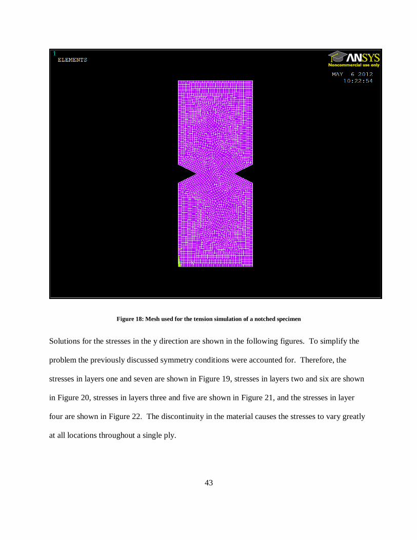
43

Figure 18: Mesh used for the tension simulation of a notched specimen

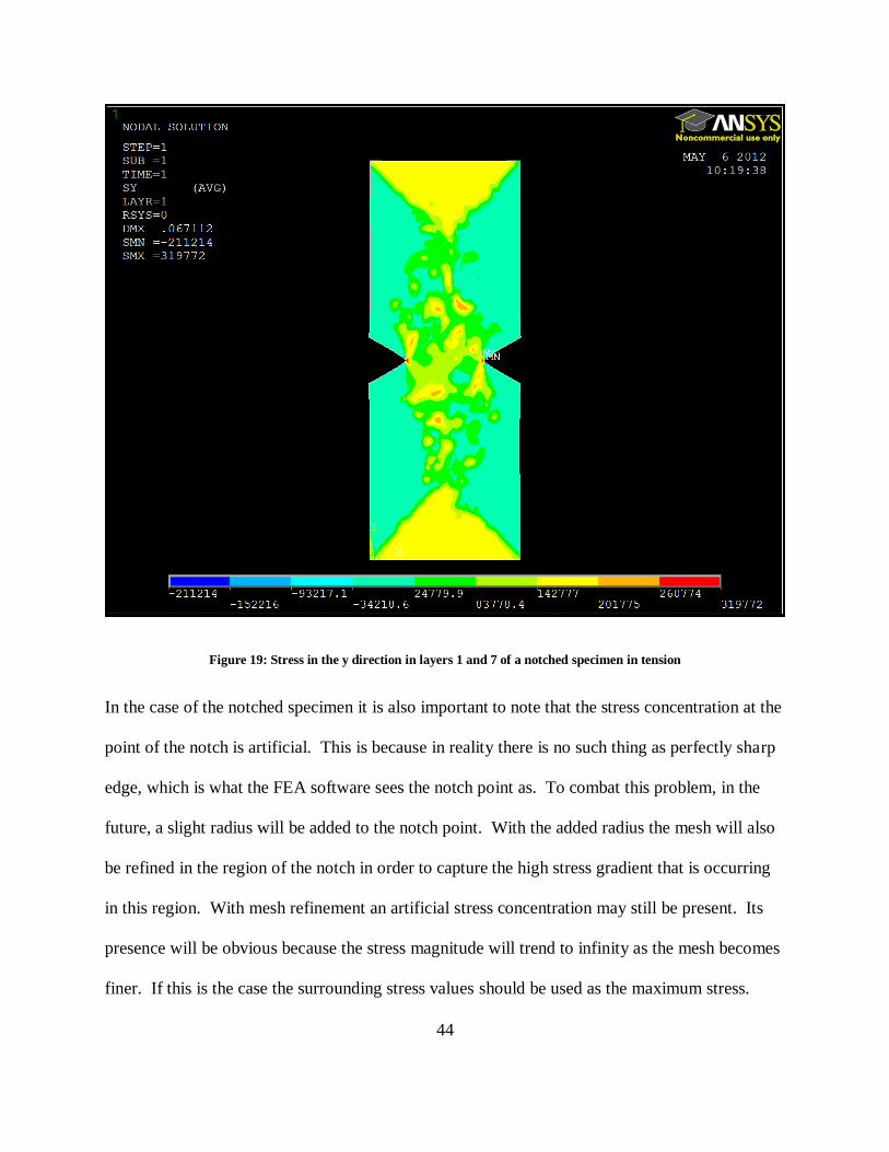
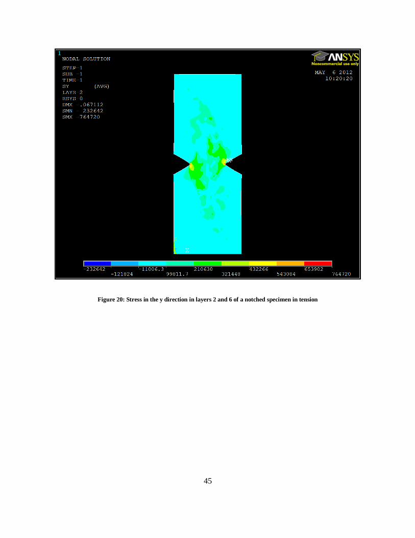
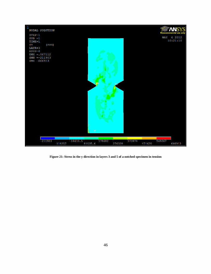
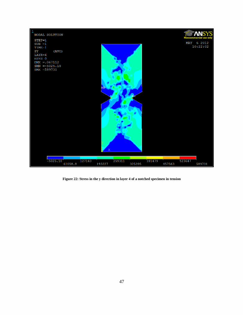
Solutions for the stresses in the y direction are shown in the following figures. To simplify the

problem the previously discussed symmetry conditions were accounted for. Therefore, the

stresses in layers one and seven are shown in Figure 19, stresses in layers two and six are shown

in Figure 20, stresses in layers three and five are shown in Figure 21, and the stresses in layer

four are shown in Figure 22. The discontinuity in the material causes the stresses to vary greatly

at all locations throughout a single ply.

44

Figure 19: Stress in the y direction in layers 1 and 7 of a notched specimen in tension

In the case of the notched specimen it is also important to note that the stress concentration at the

point of the notch is artificial. This is because in reality there is no such thing as perfectly sharp

edge, which is what the FEA software sees the notch point as. To combat this problem, in the

future, a slight radius will be added to the notch point. With the added radius the mesh will also

be refined in the region of the notch in order to capture the high stress gradient that is occurring

in this region. With mesh refinement an artificial stress concentration may still be present. Its

presence will be obvious because the stress magnitude will trend to infinity as the mesh becomes

finer. If this is the case the surrounding stress values should be used as the maximum stress.

45


46


47

Figure 22: Stress in the y direction in layer 4 of a notched specimen in tension

48

6 Conclusions

The purpose of the research discussed throughout this thesis was to investigate and determine the

composite modeling capabilities of commercial FEA software. The selected software packages

were ANSYS and Abaqus, chosen because of their availability at The Ohio State University.

The research provided insight on the mechanical responses orthotropic material and how to

properly construct FEA models of CFRPs in each of the aforementioned software packages.

6.1 Contributions

This research will help add to the knowledge base of FEA of composite materials. It proves that

FEA is accurate to current laminate theory and the results are independent of the software

package used to obtain them. Therefore, only one software package can be selected based on

ease of use instead of its accuracy.

6.2 Additional Applications

The approach discussed for modeling composites is applicable to many situations. It could be

applied to geometries like the ones discussed in chapter 5. This approach is also not limited to

tension tests. Samples that under go transverse loads can also be modeled quite easily using

these methods.

Three dimensional parts can also be modeled using shell sections. For example the shell sections

can be applied to an airplane fuselage, a wing, body panels on automobiles, automobile hoods,

etc. As long as the part is thin enough it can be meshed using shells.

49

6.3 Future Work

Modeling composite materials is more difficult than modeling traditional materials. Therefore,

predicting the point at which a CFRP will fail is also more difficult. ANSYS and Abaqus do

have built in failure theories that can be used with the shell sections, but they will not show any

detail about the failure. For example, one type of failure of a composite laminate is known as

delamination. Delamination occurs when the plies of the laminate begin to separate from each

other. Shell sections would not be able to accurately predict this type of failure because they are

not detailed enough to show how the plies will interact with each other. To model this type of

failure another method must be used. Since part of the future work will be predicting a failure of

a CFRP it will be important to learn how to model delamination.

Knowledge gained form this project will also be used to create models that attempt to match

experimental tests. Matching experimental test results would help further validate FEA and help

develop more accurate techniques of modeling composites. This knowledge could then be used

to optimize the design process of composite parts.

6.4 Summary

This project has investigated and compared the modeling capabilities of ANSYS and Abaqus,

compared the mechanical reactions of three different lay-up patterns, and verified all of this with

current laminate theory. Following verification the discussed techniques were applied to

simulate tension tests of a holed and notched specimen. The modeling techniques discussed

throughout this document increase the knowledge base of modeling composite materials and can

be implemented to help verify experimental tests and design parts for aircraft or automobiles.

50

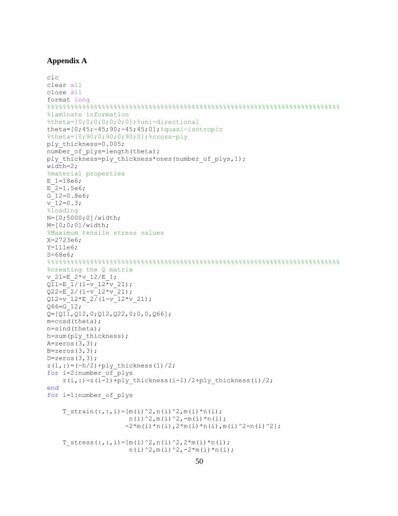
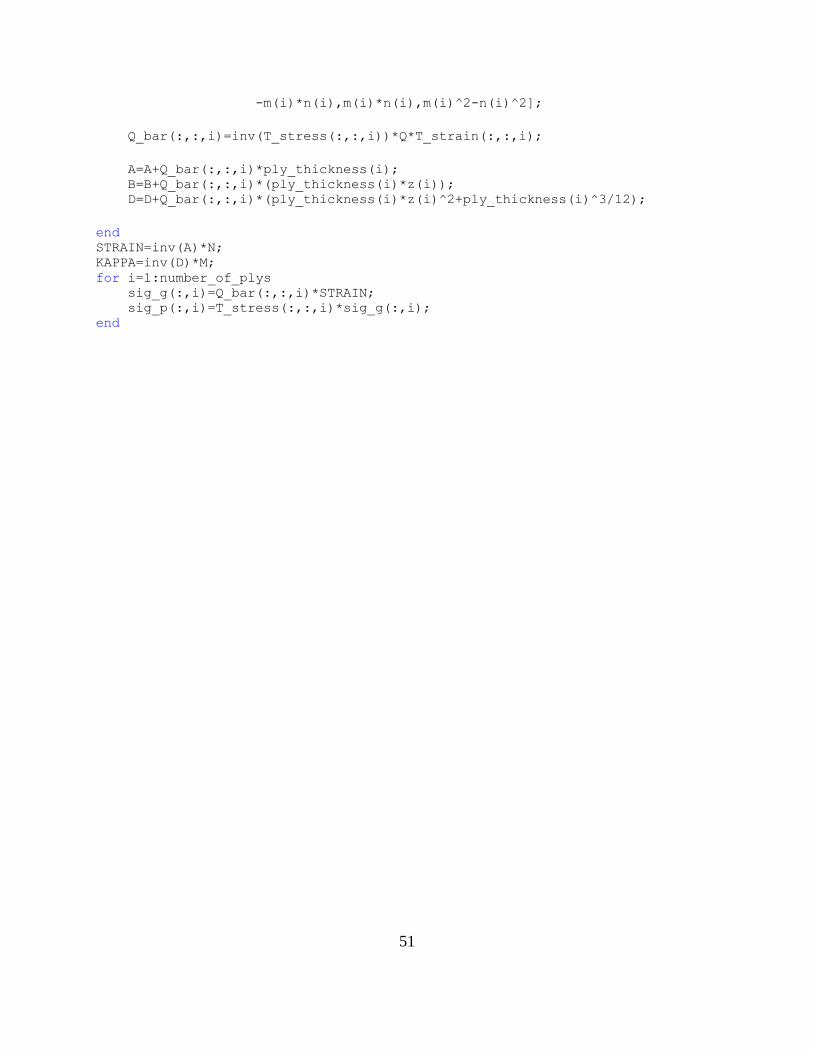
Appendix A

clc clear all close all format long %%%%%%%%%%%%%%%%%%%%%%%%%%%%%%%%%%%%%%%%%%%%%%%%%%%%%%%%%%%%%%%%%%%%%%%%%%% %laminate information %theta=[0;0;0;0;0;0;0];%uni-directional theta=[0;45;-45;90;-45;45;0];%quasi-isotropic %theta=[0;90;0;90;0;90;0];%cross-ply ply_thickness=0.005; number_of_plys=length(theta); ply_thickness=ply_thickness*ones(number_of_plys,1); width=2; %material properties E_1=18e6; E_2=1.5e6; G_12=0.8e6; v_12=0.3; %loading N=[0;5000;0]/width; M=[0;0;0]/width; %Maximum tensile stress values X=2723e6; Y=111e6; S=68e6; %%%%%%%%%%%%%%%%%%%%%%%%%%%%%%%%%%%%%%%%%%%%%%%%%%%%%%%%%%%%%%%%%%%%%%%%%%% %creating the Q matrix v_21=E_2*v_12/E_1; Q11=E_1/(1-v_12*v_21); Q22=E_2/(1-v_12*v_21); Q12=v_12*E_2/(1-v_12*v_21); Q66=G_12; Q=[Q11,Q12,0;Q12,Q22,0;0,0,Q66]; m=cosd(theta); n=sind(theta); h=sum(ply_thickness); A=zeros(3,3); B=zeros(3,3); D=zeros(3,3); z(1,:)=(-h/2)+ply_thickness(1)/2; for i=2:number_of_plys z(i,:)=z(i-1)+ply_thickness(i-1)/2+ply_thickness(i)/2; end for i=1:number_of_plys

T_strain(:,:,i)=[m(i)^2,n(i)^2,m(i)*n(i); n(i)^2,m(i)^2,-m(i)*n(i); -2*m(i)*n(i),2*m(i)*n(i),m(i)^2-n(i)^2];

T_stress(:,:,i)=[m(i)^2,n(i)^2,2*m(i)*n(i); n(i)^2,m(i)^2,-2*m(i)*n(i);

51

-m(i)*n(i),m(i)*n(i),m(i)^2-n(i)^2];

Q_bar(:,:,i)=inv(T_stress(:,:,i))*Q*T_strain(:,:,i);

A=A+Q_bar(:,:,i)*ply_thickness(i); B=B+Q_bar(:,:,i)*(ply_thickness(i)*z(i)); D=D+Q_bar(:,:,i)*(ply_thickness(i)*z(i)^2+ply_thickness(i)^3/12);

end STRAIN=inv(A)*N; KAPPA=inv(D)*M; for i=1:number_of_plys sig_g(:,i)=Q_bar(:,:,i)*STRAIN; sig_p(:,i)=T_stress(:,:,i)*sig_g(:,i); end

52

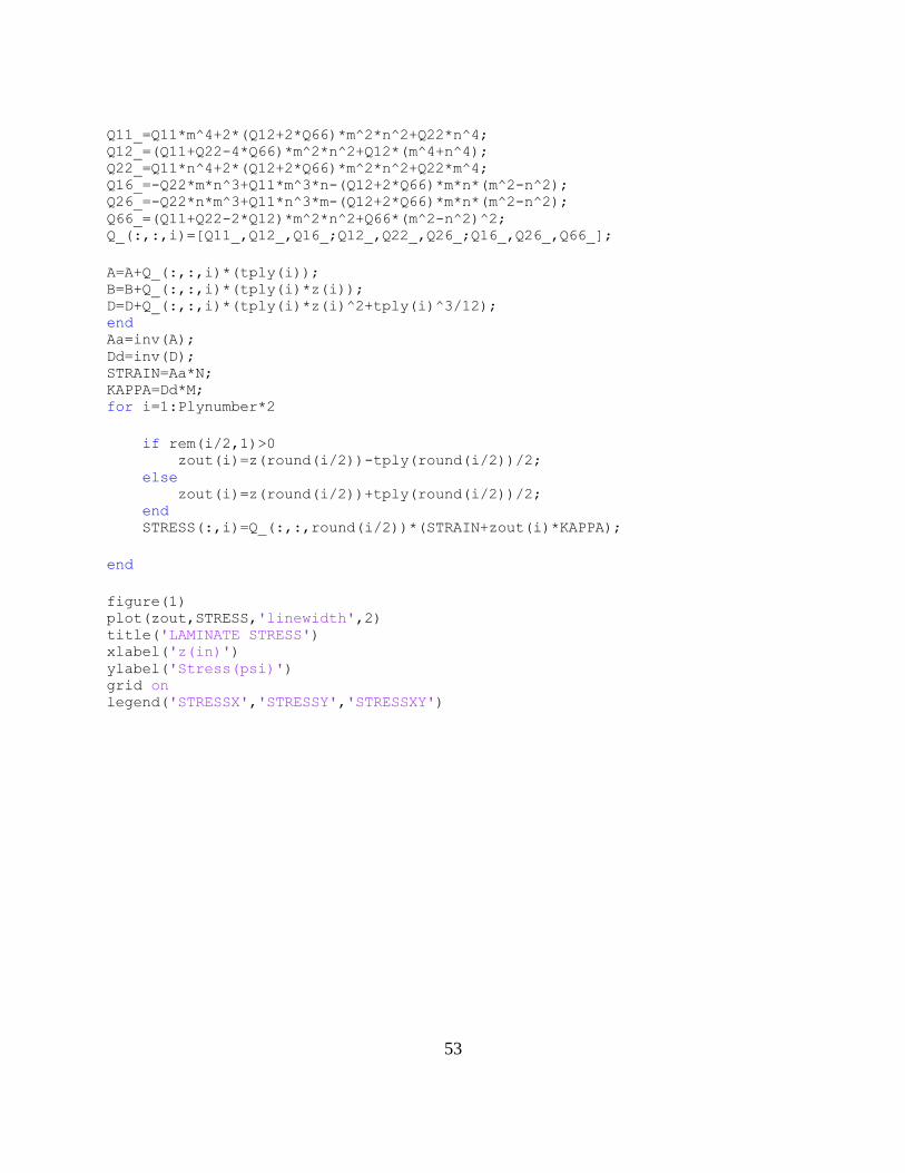
Appendix B %Undergraduate Thesis %Code Provided By Brooks Marquette %Modified by Brice Willis %7 ply tesion test %uni-directional clc clear all close all %inputs start %please enter the following values specific to the lamina of interest tply=0.005; %ply thickness Plynumber=7;%number of plys tply=tply*ones(Plynumber,1);%Will need to specify individual plies if

different thickness %enter the orientation of each ply in order from 1 to n %theta=[90;90;90;90;90;90;90]; %theta=[0;0;0;0;0;0;0]*pi/180;%uni-directional theta=[0;45;-45;90;-45;45;0]*pi/180;%quasi-isotropic %theta=[0;90;0;90;0;90;0]*pi/180;%cross-ply %elastic parameters taken from Feraboli E1=18e6; E2=1.5e6; G12=0.8e6; %Vf=0.7; v12=0.3; v21=E2*v12/E1; w=2; %Width of sample N=[0;5000;0]/w; %Tensile applied Stess M=[0;0;0]/w; %Bending Moment Stress %inputs end

h=sum(tply); A=zeros(3,3); B=zeros(3,3); D=zeros(3,3);

for i=1:Plynumber m=cos(theta(i)); n=sin(theta(i));

z(1,:)=(-h/2)+tply(1)/2; if i>=2 z(i,:)=z(i-1)+tply(i-1)/2+tply(i)/2; end

% To create Q Bar matrix and ABD matrix

Q11=E1/(1-v12*v21); Q22=E2/(1-v12*v21); Q12=v12*E2/(1-v12*v21); Q66=G12;

53

Q11_=Q11*m^4+2*(Q12+2*Q66)*m^2*n^2+Q22*n^4; Q12_=(Q11+Q22-4*Q66)*m^2*n^2+Q12*(m^4+n^4); Q22_=Q11*n^4+2*(Q12+2*Q66)*m^2*n^2+Q22*m^4; Q16_=-Q22*m*n^3+Q11*m^3*n-(Q12+2*Q66)*m*n*(m^2-n^2); Q26_=-Q22*n*m^3+Q11*n^3*m-(Q12+2*Q66)*m*n*(m^2-n^2); Q66_=(Q11+Q22-2*Q12)*m^2*n^2+Q66*(m^2-n^2)^2; Q_(:,:,i)=[Q11_,Q12_,Q16_;Q12_,Q22_,Q26_;Q16_,Q26_,Q66_];

A=A+Q_(:,:,i)*(tply(i)); B=B+Q_(:,:,i)*(tply(i)*z(i)); D=D+Q_(:,:,i)*(tply(i)*z(i)^2+tply(i)^3/12); end Aa=inv(A); Dd=inv(D); STRAIN=Aa*N; KAPPA=Dd*M; for i=1:Plynumber*2

if rem(i/2,1)>0 zout(i)=z(round(i/2))-tply(round(i/2))/2; else zout(i)=z(round(i/2))+tply(round(i/2))/2; end STRESS(:,i)=Q_(:,:,round(i/2))*(STRAIN+zout(i)*KAPPA);

end

figure(1) plot(zout,STRESS,'linewidth',2) title('LAMINATE STRESS') xlabel('z(in)') ylabel('Stress(psi)') grid on legend('STRESSX','STRESSY','STRESSXY')

54

References

Anonymous. (2008). Abaqus/CAE User's Manual. Providence, RI, USA.

Anonymous_2. (2009). ANSYS Help System version 12.0. Canonsburg, PA, USA: ANSYS.

Ashby, M. F. (2005). Materials Selection in Mechanical Design. Burlington: Elsevier.

Feraboli, P., & Kedward, K. T. (2003). Four-point bend interlaminar shear testing of uni- and

multi-directional carbon/epoxy composite systems. Composites: Part A.

Miracle, D. B., & Donaldson, S. L. (2001). ASM Handbook, Volume 21-Composites. In D. B.

Miracle, & S. L. Donaldson, ASM Handbook, Volume 21-Composites. ASM

International.

Staab, G. H. (1999). Laminar Composites. Woburn: Butterworth-Heinemann.

Swanson, S. R. (1997). Introduction to Design and Analysis with Advanced Composite

Materials. Upper Saddle River: Simon & Schuster.

Unknown. (2008). Why Carbon Fiber. Retrieved March 2012, from Plasan Carbon Composites:

http://www.plasancarbon.com/template/default.aspx?catid=2&PageId=18

composite modeling capabilities of commercial finite ... · pdf filecomposite modeling...

Documents