composite likelihood methods for space - journ©es mas 2008

www.dst.unive.it\ ∼gaetan

Composite likelihood methods for space(and space-time) covariance models

Carlo Gaetan

Dipartimento di StatisticaUniversita Ca’ Foscari Venezia 1

Rennes, 27-29 August 2008

1Joint work with M. Bevilacqua† ,J. Mateu‡, E. Porcu‡ ( † Universita Ca’Foscari - Venezia, Italy, ‡ Universitat Jaume I, Castellon, Spain).

Journees MAS de la SMAI 1/ 29


Outline of the talk

Geostatistical approach

Estimation methods

(Weighted) composite likelihood method

Model selection criterion

Conclusions



Geostatistical approach I

• Z = {Z (s, t)}, spatio-temporal Random Fields (RFs), s ∈ Rd

is a spatial location, t ∈ R is a time point

Z (s, t) = µ(s, t) + ε(s, t)

data = large scale + small scale

• Assumption: µ(s, t) known (µ(s, t) = 0) and E[Z (s, t)]2 < ∞.

• Space-time covariance function

cov(Z (s1, t1), Z (s2, t2))



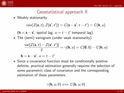
Geostatistical approach II• Weakly stationarity

cov(Z (s, t), Z (s′, t ′)) = C (s − s′, t − t ′) = C (h, u)

(h = s − s′, spatial lag, u = t − t ′ temporal lag).

• The (semi) variogram (under weak stationarity)

var[Z (s, t) − Z (s′, t ′)]

2= γ(h, u) = C (0, 0) − C (h, u)

h = s − s′, u = t − t ′

• Since a covariance function must be conditionally positivedefinite, practical estimation generally requires the selection ofsome parametric class of covariance and the correspondingestimation of these parameters.

γ(h, u; θ) ⇐⇒ C (h, u; θ)



WLS method (Cressie, 1985)

• Non parametric estimation of γ(h, u)

γ(h, u) =1

2|N(h, u)|

∑

(si ,sj ;ti ,tj )∈N(h,u)

(Z (si , ti ) − Z (sj , tj)2

where N(h, u) is some specified tolerance region around h andu (bin).

•

θ = argminθ∈Θ

m∑

k=1

|N (hk , uk) |

γ2(hk , uk ; θ)(γ(hk , uk) − γ(hk , uk ; θ))2 ,



Maximum likelihood (ML) estimation

• Data: single realization Z = (Z (s1, t1), . . . ,Z (sn, tn))′ from a

space-time random field .

• {Z (s, t)} is zero mean Gaussian field. The log-likelihood

l(θ) = −1

2log detΣ(θ) −

1

2Z′Σ(θ)−1Z

where Σ(θ) = cov(Z).

• Difficulties: for Gaussian random fields, the most critical partof the likelihood calculation is to evaluate the determinantand inverse of the covariance matrix. Each calculation of thelikelihood requires O(n3) steps.



Composite likelihoods

General idea

1. Let Z = (Z1, . . . ,Zn)′ be a n-dimensional vector random

variable with density f (Z; θ) for some unknown parameterθ ∈ Θ ⊆ R

d .

2. Suppose that the joint distribution of Y is difficult toevaluate, but that it is possible to compute likelihoods forsome subsets of the data.

3. It may be expedient to consider instead a pseudolikelihoodcompounding such likelihood objects.

4. This idea dates back to Besag (1974) and it has been termedcomposite likelihood after Lindsay (1988).



Composite likelihood: definition

Consider

1. a parametric model{f (Z; θ),Z ∈ Z ⊆ R

n, θ ∈ Θ ⊆ Rp};

2. a set of measurable events {Ai ; i = 1, . . . ,m}.

Then, a composite likelihood (CL) is the weighted product of thelikelihoods corresponding to each single event,

CL(θ) = CL(θ;Z) =m∏

i=1

f (Z ∈ Ai ; θ)wi ,

where {wi ; i = 1, . . . ,m} are positive weights.Its maximum, if unique, is the maximum composite likelihood

estimator (MCLE).



Vecchia (1988)’s approximation (spatial case)

• The exact joint density of Z may be written as

f (Z; θ) = f (Z (s1); θ)n∏

i=2

f (Z (si )|Z (si−1), . . . ,Z (s1); θ)

where the ordering of observations is arbitrary.• Replace

f (Z (si )|Z (si−1), . . . ,Z (s1); θ) by f (Z (si )|Z(Ni ); θ),

where Z(Ni ) is some subset of {Z (si−1), . . . ,Z (s1)} and|Z(Ni )| is not too large.

CL(θ) =n∏

i=1

f (Z (si )|Z(Ni ); θ)

• Each Z(Ni ) consisted of a number of near neighbors of Z (si ) ,though the precise choice of Z(Ni ) was arbitrary.



Stein et al. (2004)’s approximation

• It might be more efficient to do it in blocks, evaluatingconditional densities of the form

f (Z (si ), . . . ,Z (si+k)|Z(Ni ); θ)

• It is not necessarily best to choose Z(Ni ) consisting only ofnear neighbours of the observation or observations whoseconditional density is being evaluated.

• There is an extension to the space-time data for regularmonitoring on time (Stein, 2005).



Caragea and Smith (2006)’s approximation

‘Small blocks method’:

• The observation locations are grouped into blocks Ni ,i = 1, . . . , k of roughly the same size.

• For each block, compute the joint density of all observationsin that block f (Z(Ni ); θ)

• The small blocks likelihood is the product of joint densities forall the blocks, treating the blocks as if they were mutuallyindependent.

CL(θ) =k∏

i=1

f (Z(Ni ); θ)

• No extension to space-time data



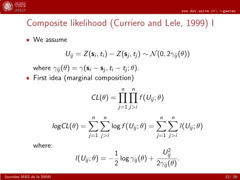
Composite likelihood (Curriero and Lele, 1999) I

• We assume

Uij = Z (si , ti ) − Z (sj , tj) ∼ N (0, 2γij(θ))

where γij(θ) = γ(si − sj , ti − tj ; θ).

• First idea (marginal composition)

CL(θ) =

n∏

j=1

n∏

j>i

f (Uij ; θ)

logCL(θ) =n∑

j=1

n∑

j>i

log f (Uij ; θ) =n∑

j=1

n∑

j>i

l(Uij ; θ)

where:

l(Uij ; θ) = −1

2log γij(θ) +

U2ij

2γij(θ).



Composite likelihood (Curriero and Lele, 1999) II

Features:

• Similar to WLS, but unlike WLS, it does not require anysubjective choice of the lag bins.

• The number of operations requested is O(n2).

• To obtain estimates of θ we maximise the function CL(θ) orequivalently solve the estimating equation

vCL(θ) =n∑

i=1

n∑

j>i

∇l(Uij ; θ) =n∑

i=1

n∑

j>i

∇γij(θ)

γij(θ)

(1 −

U2ij

2γij(θ)

)= 0.

• Estimating unbiased equation, irrespectively of thedistributional assumptions imposed on Uij .



Optimal estimating equation

Second idea: optimal estimating equation

• If the fourth-order joint distributions of Uij is known it wouldbe possible to come up with an optimal way of combining theindividual score vCL(θ):

(E∇vCL(θ))T [Cov(vCL(θ))]

−1vCL(θ) = 0.

• The covariance matrix Cov(vCL(θ)) has dimension n2 × n2,and its inversion is computationally prohibitive for large n.



Weighted composite likelihood

• Our idea: instead of searching optimal weights we consider

WCL(θ,d) =1

Wn,d

n∑

i

n∑

j>i

l(Uij ; θ)wij(d),

or

v(θ,d) =1

Wn,d

n∑

i

n∑

j>i

∇l(Uij ; θ)wij(d) = 0,

where

wij(d) =

{1 ‖si − sj‖ ≤ ds , |ti − tj | ≤ dt , d = (ds , dt)

′

0 otherwise

and Wn,d =∑n

i

∑nj>i wij(d).

• We look for an “optimal lag” d∗.



A measure of efficiency

How to choose d ? We look at the Godambe information matrix

G (θ,d) = H(θ,d)J(θ,d)−1H(θ,d)′,

whereH(θ,d) = E[∇v(θ,d)]

andJ(θ,d) = E[v(θ,d)v(θ,d) ′]

In our case

H(θ, d) = E[∇eWCL(θ, d)] =1

Wn,d

X

i

X

j>i

(∇γij

γij

∇γ′

ij

γij

)wij (d)

J(θ, d) = E[eWCL(θ, d)eWCL(θ, d)′] =

2

W 2n,d

X

i

X

j>i

X

l

X

k>l

∇γ′

ij

γij

∇γ′

lk

γlk

ρijlkwij (d)wlk (d)

where ρijlk = Corr(U2ij , U2

lk )

Under Gaussianity:

ρijlk = Corr(U2ij , U

2lk ) =

(γil − γjl − γjk + γik )2

4γij γlk

(1)



Asymptotics I

We suppose

• θ ∈ Θ ⊂ Rp, Θ compact set;

• increasing domain asymptotics R0 = (−12 , 1

2 ]d+1,Rn = {(s1, t1), . . . , (sn, tn)} = (nR0) ∩ Z

d+1

• M = {(h1, u1), . . . , (hK , uK )}, K ≥ p is a finite set notcontaining the origin and which determines which pairs ofobservations contribute to the sum;

• γ(h; θ) is twice continuously differentiable for θ ∈ V , V is aneighbourhood of the true value θ0;

• Γ(θ) = [∇γ(h1, u1; θ), . . . ,∇γ(hK , uK ; θ)] has full rank

•∑K

i=1(2γ(hi , ui ; θ1) − 2γ(hi , ui ; θ2)) > 0 for all θ1 6= θ2,(identifiability condition);

• a mixing conditions on {Z (s, t)}



Asymptotics II

then (Guyon, 1995)

• −WCL(θ) is an additive contrast function;

• θWCL is consistent and asymptotically Gaussian

G (θ,d)1/2(θWCL − θ0)d

−→ N (0, Ip)

i.e.

(θWCL − θ0) ≈ N (0, G (θ,d)−1)



A simple spatial example

1. Exponential model

C (h; θ) = exp

(−3

‖h‖

θ

), θ > 0. (2)

0 1 2 3 4

0.0

0.5

1.0

1.5

2.0

2.5

3.0

3.5

distance

Inve

rse

of G

odam

be In

form

atio

n θ = 3θ = 2θ = 1

0 1 2 3 4 5 60.

00.

51.

01.

52.

02.

53.

03.

5

distance

Inve

rse

of G

odam

be In

form

atio

n

θ = 3θ = 2θ = 1

(a) (b)

(a) 49 points located on a 7 × 7 regular grid [0, 0.5, . . . , 3]2;(b) 49 points uniformly distributed on [0, 3]2.



Weighted composite likelihood: practicalimplementation

• First step:We choose the ‘lag’ d minimising the G−1(θ,d) in the partialorder of nonnegative definite matrices or equivalently

d∗ = argmind∈D

tr(G−1(θ,d)), (3)

where D is a set of lags.◮ Get a consistent estimate for θ (for instance θWLS)◮ Computation of J(θWLS ,d) becomes quickly infeasible

(O(n4)). Estimation through sub-sampling technique.

• Second step:

θWCL = argminθ∈Θ

WCL(θ,d∗) (4)



Computational burden

Method Complexity Drawbacks

Likelihood O(n3) unfeasible for large data-setVecchia & Stein O(n) subjective conditional sets choiceCaragea & Smith O(n2) subjective size of the block

WCLIC O(W 2n,d∗) a preliminary estimation



A space-time example I

300 independent simulations from a zero mean Gaussian processon

• a space-time lattice S × T , with◮ S = {1, 1.5, 2, . . . ,N}2 and N = 3, 4, 5

S

◮ T = {1, . . . ,T} and T = 15, 30, 45



A space-time example II

• a non separable covariance model:

C(h, u) =1

(a|u| + 1)exp

(−

c‖h‖

(a|u| + 1)0.25

), a = c = 2

MSE Relative efficiency for WLS, CL and WCL estimationmethods with respect to ML.

n = 25 n = 49 n = 81WLS CL WCL WLS CL WCL WLS CL WCL

c 12.96 16.33 4.17 21.83 28.69 4.39 28.51 37.61 7.10T = 15 a 12.85 21.59 4.38 20.35 30.53 4.92 25.19 33.71 6.95

c 19.23 23.95 4.32 26.01 32.59 6.79 33.53 41.81 7.30T = 30 a 25.34 40.91 5.23 33.39 46.59 5.79 39.91 49.95 7.23

c 20.25 25.05 4.85 33.04 41.54 6.56 39.10 47.97 8.01T = 45 a 27.34 41.83 4.35 40.96 51.12 5.18 46.86 58.53 6.42



Model selection criterion

• Model selection criteria as AIC and BIC depend on thecomputation of the likelihood function.

• We follow (Varin and Vidoni, 2005) and we select the modelmaximizing

WCLIC (θWCL) = WCL(θWCL) + tr(JH−1), (5)

where J and H are consistent estimates of J and H.

• If WCL = L the the selection statistic reduces to the Akaikecriterion

l(θML) − dim(θ)



WCLIC: a simulation study

• 100 independent simulations from a zero mean space-timegaussian process with covariance models:

C(h, u) =σ2

(a|u|2α + 1)exp

(−

c‖h − εuv‖2γ)

(a|u|2α + 1)βγ

). (6)

1. A –Separable model (β = 0, ε = 0)2. B –Non separable model (ε = 0)3. C –Asymmetric in time non separable model

• S regular spaced grid on a square [1, 4]2 equally spaced by 1(i.e. 16 locations) and T = {1, . . . , 150}

IdentifiedA B C

A 81 14 5True B 6 80 14

C 3 11 86



Conclusions

• WCL seems to be a valid compromise between thecomputational burdens of ML and the loss of efficiency ofWLS.

• Godambe information as natural criteria for the optimaldistance for the WCL.

• Model selection is feasible for WCL.



Merci !



References I

Besag, J. (1974) Spatial interaction and the statistical analysis of latticesystems (with discussion). Journal of the Royal Statistical Society B,36, 192–236.

Caragea, P. and Smith, R. (2006) Approximate likelihoods for spatialprocesses. Tech. rep., Department of Statistics, Iowa State University.

Cressie, N. (1985) Fitting variogram models by weighted least squares.Mathematical Geology, 17, 239–252.

Curriero, F. and Lele, S. (1999) A composite likelihood approach tosemivariogram estimation. Journal of Agricultural, Biological and

Environmental Statistics, 4, 9–28.

Guyon, X. (1995) Random Fields on a Network: Modeling, Statistics and

Applications. New York: Springer.

Lindsay, B. (1988) Composite likelihood methods. Contemporary

Mathematics, 80, 221–239.



References II

Stein, M. (2005) Statistical methods for regular monitoring data. Journal

of the Royal Statistical Society B, 67, 667–687.

Stein, M., Chi, Z. and Welty, L. (2004) Approximating likelihoods forlarge spatial data sets. Journal of the Royal Statistical Society B, 66,275–296.

Varin, C. and Vidoni, P. (2005) A note on composite likelihood inferenceand model selection. Biometrika, 52, 519–528.

Vecchia, A. (1988) Estimation and model identification for continuousspatial processes. Journal of the Royal Statistical Society B, 50,297–312.


composite likelihood methods for space - journ©es mas 2008

Documents