component-level parallelization of triangular decompositionsmmorenom/publications/msri-2007.pdf ·...
TRANSCRIPT

Component-level Parallelization of TriangularDecompositions
Marc Moreno Maza & Yuzhen Xie
University of Western Ontario, Canada
February 1, 2007
Interactive Parallel Computation in Support of Research in Algebra,
Geometry and Number Theory
MSRI Workshop 2007, Berkeley.
1
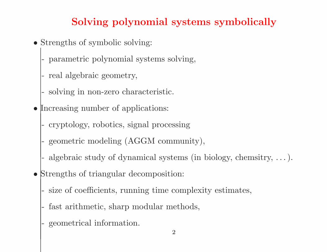
Solving polynomial systems symbolically
• Strengths of symbolic solving:
- parametric polynomial systems solving,
- real algebraic geometry,
- solving in non-zero characteristic.
• Increasing number of applications:
- cryptology, robotics, signal processing
- geometric modeling (AGGM community),
- algebraic study of dynamical systems (in biology, chemsitry, . . . ).
• Strengths of triangular decomposition:
- size of coefficients, running time complexity estimates,
- fast arithmetic, sharp modular methods,
- geometrical information.2

Grobner bases and triangular decompositions
x2 + y + z = 1
x + y2 + z = 1
x + y + z2 = 1
has Grobner basis :
z6 − 4z4 + 4z3 − z2 = 0
2z2y + z4 − z2 = 0
y2 − y − z2 + z = 0
x + y + z2 − 1 = 0
and triangular decomposition :
z = 1
y = 0
x = 0
⋃
z = 0
y = 1
x = 0
⋃
z = 0
y = 0
x = 1
⋃
z2 + 2z − 1 = 0
y = z
x = z
3

Triangular decompositions
• The zero set V (F ) admits a decomposition (unique when minimal)
V (F ) = V (F1)∪ · · · ∪V (Fe),
s.t. F1, . . . , Fe ⊂ K[X ] and every V (Fi) cannot be decomposed further.
• Moreover, up to technical details, each V (Fi) is the zero set of a
triangular system, which can view as a solved system
Tn(x1, . . . , xd, xd+1, xd+2, . . . , xn−1,xn) = 0
Tn1(x1, . . . , xd, xd+1, xd+2, . . . ,xn−1) = 0
...
Td+2(x1, . . . , xd, xd+1,xd+2) = 0
Td+1(x1, . . . , xd,xd+1) = 0
h(x1, . . . , xd) 6= 0
4

Parallelizing the computation of Grobner bases
Input: F ⊂ K[X ] and an admissible monomial ordering ≤.
Output: G a reduced Grobner basis w.r.t. ≤ of the ideal 〈F 〉
generated by F .
repeat
(S) B := MinimalAutoreducedSubset(F, ≤)
(R) A := S Polynomials(B)∪F ;
R := Reduce(A, B, ≤)
(U) R := R \ {0}; F := F ∪R
until R = ∅
return B
5

The parallel characteristic set method
Input: F ⊂ K[X ].
Output: C an autoreduced characteristic set of F (in the sense of Wu).
repeat
(S) B := MinimalAutoreducedSubset(F, ≤)
(R) A := F \ B;
R := PseudoReduce(A, B, ≤)
(U) R := R \ {0}; F := F ∪R
until R = ∅
return B
• Repeated calls to this procedure computes a decomposition of V (F ).
• Cannot start computing the 2nd component before the 1st is completed.
6

Solving polynomial systems symbolically and in
parallel!
• Related work :
- Parallelizing the computation of Grobner bases (R. Bundgen,
M. Gobel & W. Kuchlin, 1994) (S. Chakrabarti & K. Yelick, 1993 -
1994) (G. Attardi & C. Traverso, 1996) (A. Leykin, 2004)
- Parallelizing the computation of characteristic sets (I.A. Ajwa, 1998),
(Y.W. Wu, W.D. Liao, D.D. Liu & P.S. Wang, 2003) (Y.W. Wu,
G.W. Yang, H. Yang, H.M. Zheng & D.D. Liu, 2005)
7

Solving polynomial systems symbolically and in
parallel!
• New motivations:
– renaissance of parallelism,
– new algorithms offering better opportunities for parallel execution.
• Our goal:
– multi-level parallelism:
∗ coarse grained “component-level” for tasks computing geometric
objects,
∗ medium/fine grained level for polynomial arithmetic within each
task.
– to develop a solver for which the number of processes in use
depends on the geometry of the solution set
8

Ideally:
Processor P0
x2 + y + z = 1
x + y2 + z = 1
x + y + z2 = 1
Processor P1
z = 1
y = 0
x = 0
Processor P2
z = 0
y = 1
x = 0
Processor P3
z = 0
y = 0
x = 1
Processor P4
z2 + 2z − 1 = 0
y = z
x = z
9

Dynamic and very irregular computations (1/2)
• How do splits occur during decompositions? Given a polynomial ideal I
and polynomials p, a, b, there are two rules:
• I 7−→ (I + p, I : p∞).
• I + 〈a b〉 7−→ (I + 〈a〉, I + 〈b〉).
• The second one is more likely to split computations evenly. But
geometrically, it means that a component is reducible.
• Unfortunately, most polynomial systems F ⊆ Q[X ] are equiprojectable,
that is, they can be represented by a single triangular set.
- This is true in theory, shape lemma: (Becker, Mora, Marinari &
Traverso, 1994).
- and in practice: SymbolicData.org.
• However, for F ⊆ Z/pZ[X ] where p prime, the second rule is more likely
to be used.10

Dynamic and very irregular computations (2/2)
• Very irregular tasks (CPU time, memory, data-communication)
T4
T0
T1 T2
T3T5
T9T8T7
T6
11

Initial task [{f1, f2, f3}, ∅]
f1 = x − 2 + (y − 1)2
f2 = (x − 1)(y − 1) + (x − 2)y
f3 = (x − 1)z
y = 0
x = 1
x − 1 + y2− 2y = 0
(2y − 1)x + 1 − 3y = 0
z = 0
z = 0
y = 0
x = 1
z = 0
y = 1
x = 2
z = 0
2y = 3
4x = 7
12

Even worse: redundant and irregular tasks
x
4
4
2
2
−2−4
0
y
5
5
31
3
0−1−3
1
−5−1
−2
−3
−4
−5
The red and blue surfaces intersect on the line x − 1 = y = 0 contained in
the green plane x = 1. With the other green plane z = 0, they intersect at
(2, 1, 0), ( 7
4, 3
2, 0) but also at x − 1 = y = z = 0, which is redundant.
13

How to create and exploit parallelism?
• We start from an algorithm (Triade, MMMM 2000)
- based on incremental solving for exploiting geometrical information,
- solving by decreasing order of dimension for removing redundant
components efficiently.
• This algorithm
- uses a task model for the intermediate computations,
- but a naive parallelization would be unsuccessful, for the reasons
mentioned earlier.
• So, we rely also
- on the modular algorithm (Dahan, MMM, Schost, Wu and Xie, 2005)
- in order to create opportunities for parallel execution with input
systems over Q.
• We adapt the Triade algorithm to exploit the opportunities created by
the modular techniques.14

Triangular Decompositions: a geometrical approach
Incremental solving: by solving one equation after the other, lead to a
more geometric approach
{
x2 + y + z = 1
x2 + y + z = 1
x + y2 + z = 1
x2 + y + z = 1
x + y2 + z = 1
x + y + z2 = 1
15

{
x2 + y + z = 1
x + y2 + z = 1
y4 + (2z − 2)y2
+ y − z + z2 = 0
x + y = 1
y2 − y = 0
z = 0
2x + z2 = 1
2y + z2 = 1
z3 + z2 − 3z = −1
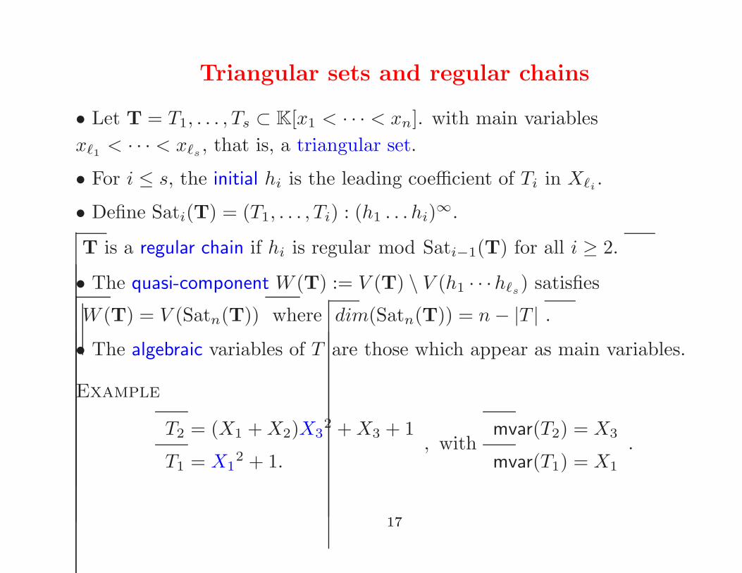
Triangular sets and regular chains
• Let T = T1, . . . , Ts ⊂ K[x1 < · · · < xn]. with main variables
xℓ1 < · · · < xℓs, that is, a triangular set.
• For i ≤ s, the initial hi is the leading coefficient of Ti in Xℓi.
• Define Sati(T) = (T1, . . . , Ti) : (h1 . . . hi)∞.
T is a regular chain if hi is regular mod Sati−1(T) for all i ≥ 2.
• The quasi-component W (T) := V (T) \ V (h1 · · ·hℓs) satisfies
W (T) = V (Satn(T)) where dim(Satn(T)) = n − |T | .
• The algebraic variables of T are those which appear as main variables.
Example
T2 = (X1 + X2)X32 + X3 + 1
T1 = X12 + 1.
, withmvar(T2) = X3
mvar(T1) = X1
.
17

Task Model
• A task is any [F, S] whith F ⊂ K[X ] finite and S ⊂ K[X ] triangular set.
• The task [F, S] is solved if F = ∅ and S is a regular chain.
• Solving [F, S] means computing regular chains T1, . . . , Te such that:
V (F ) ∩ W (S) ⊆ ∪ei=1W (Ti) ⊆ V (F ) ∩ W (S).
• [F1, S1]≺ [F2, S2] if either S1 ≺S2 or (∃f1 ∈ F1) (∀f2 ∈ F2) f1 ≺ f2 and
S1 ≃S2.
• The tasks [F1, S1], . . . , [Fe, Se] form a delayed split of [F, S] if for all
1 ≤ i ≤ e we have [Fi, Si]≺ [F, S] and the following holds
V (F ) ∩ W (S) ⊆ ∪ei=1 V (Fi) ∩ W (Si) ⊆ V (F ) ∩ W (S).
18

The main operations
• Triangularize(F, S) returns regular chains T1, . . . , Te solving [F, S].
• When F = ∅ we write Extend(S) instead of Triangularize(F, S).
• For p a polynomial and T a regular chain, Decompose(p, T ) returns a
delayed split of [{p}.T ]. Hence Decompose(p, T ) computes V (p)∩W (T ) by
lazy evaluation.
• For p, t polynomials with same main variable and T a regular chain,
GCD(p, t, T ) returns pairs (g1, T1), . . . , (ge, Te) such that
- whenever |Ti| = |T | holds, gi is a GCD of p and t modulo Ti,
- T1, . . . , Te solve T , that is, W (T ) ⊆ ∪ei=1W (Ti) ⊆ W (T ).
• RegularizeInitial(p, T ) returns regular chains T1, . . . , Te solving T and
such that p mod Sat(Ti) is constant or its initial is regular.
These operations rely on the D5 Principle (Della Dora et al., 1985).
19

The Triangularize algorithm
Input: a task [F, T ]
Output: regular chains T1, . . . , Te solving [F, T ]
Triangularize(F, T ) == generate
1 R := [[F, T ]]
2 # R is a list of tasks
3 while R 6= [ ] repeat
4 choose and remove a task [F1, U1] from R
5 F1 = ∅ =⇒ yield U1
6 choose a polynomial p ∈ F1
7 G1 := F1 \ {p}
8 for [H, T ] ∈ Decompose(p, U1) repeat
9 R := cons ([G1 ∪ H, T ], R)
20

The Decompose algorithm
Input: a polynomial p and a regular chain T such
that p 6∈ Sat(T ).
Output: a delayed split of [{p}, T ].
Decompose(p, T ) == generate
1 for C ∈ RegularizeInitial(p, T ) repeat
2 f := Reduce(p, C)
3 f = 0 =⇒ yield [∅, C]
4 f ∈ K =⇒ iterate
5 v := mvar(f)
6 v 6∈ mvar(C) =⇒ yield [{init(f), p}, C]
7 for D ∈ Extend(C ∪ {f}) repeat yield [∅, D]
8 for [F, E] ∈ AlgebraicDecompose(f, C<v ∪ C>v, Cv)
9 repeat yield [F, E]
21
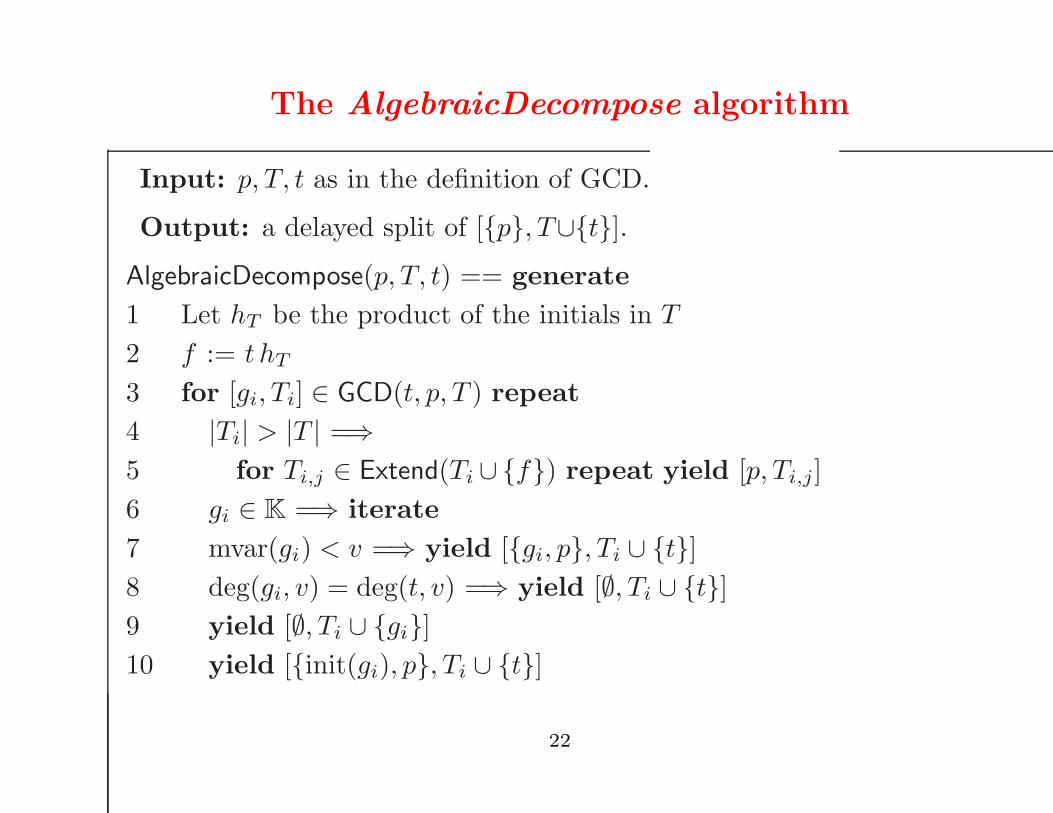
The AlgebraicDecompose algorithm
Input: p, T, t as in the definition of GCD.
Output: a delayed split of [{p}, T∪{t}].
AlgebraicDecompose(p, T, t) == generate
1 Let hT be the product of the initials in T
2 f := t hT
3 for [gi, Ti] ∈ GCD(t, p, T ) repeat
4 |Ti| > |T | =⇒
5 for Ti,j ∈ Extend(Ti ∪{f}) repeat yield [p, Ti,j]
6 gi ∈ K =⇒ iterate
7 mvar(gi) < v =⇒ yield [{gi, p}, Ti ∪ {t}]
8 deg(gi, v) = deg(t, v) =⇒ yield [∅, Ti ∪ {t}]
9 yield [∅, Ti ∪ {gi}]
10 yield [{init(gi), p}, Ti ∪ {t}]
22

Solving by decreasing order of dimension
• A task [G, C] output by Decompose(p, T ) is solved, that is G = ∅, if and
only W (C) is a component of V (p)∩W (T ) with maximum dimension.
⇒ Tasks in Triangularize can be chosen such that regular chains are
generated by decreasing order of dimension (= increasing height).
Allow efficient control of redundant components.
• To do so:
- each task [Fi, Ti] is assigned a priority based on rank and dimension
considerations.
- a task chosen in R has maximum priority.
⇒ This leads to a first parallel version of Triangularize where all tasks of
maximum priority are executed concurrently.
23

Create parallelism: Using modular techniques
Modular Solving:
O(d )3
Merging: O (d)~
2Lifting: O(d )
T0
For solving F ⊆ Q[X ] we use modular methods. Indeed, for a prime p:
• irreducible polynomials in Q[X ] are likely to factor modulo p,
• for p big enough, the result over Q can be recovered from the one over
Z/pZ[X ].
(X. Dahan, M. Moreno Maza, E. Schost, W. Wu & Y. Xie, 2005)24

Effect of modular solving
Sys Name n d p Degrees
1 eco6 6 3 105761 [1,1,2,4,4,4]
2 eco7 7 3 387799 [1,1,1,1,4,2,
4,4,4,4,4,2]
3 CassouNogues2 4 6 155317 [8]
4 CassouNogues 4 8 513899 [8,8]
5 Nooburg4 4 3 7703 [18,6,6,3,3,4,4,4,4,2,2,2,
2,2,2,2,2,1,1,1,1,1]
6 UteshevBikker 4 3 7841 [1,1,1,1,2,30]
7 Cohn2 4 6 188261 [3,5,2,1,2,1,1,16,12,10,8,8,
4,6,4,4,4,4,2,1,1,1,1,1,1,1,
1,1,1,1,1,1,1]
25
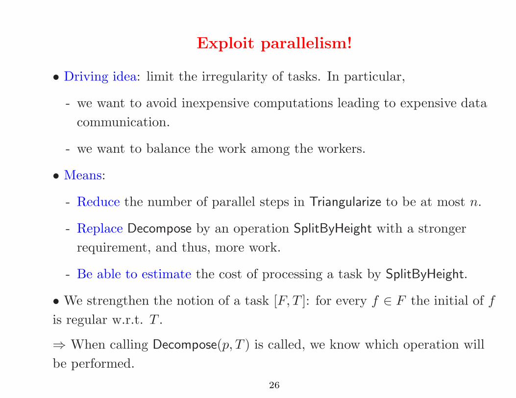
Exploit parallelism!
• Driving idea: limit the irregularity of tasks. In particular,
- we want to avoid inexpensive computations leading to expensive data
communication.
- we want to balance the work among the workers.
• Means:
- Reduce the number of parallel steps in Triangularize to be at most n.
- Replace Decompose by an operation SplitByHeight with a stronger
requirement, and thus, more work.
- Be able to estimate the cost of processing a task by SplitByHeight.
• We strengthen the notion of a task [F, T ]: for every f ∈ F the initial of f
is regular w.r.t. T .
⇒ When calling Decompose(p, T ) is called, we know which operation will
be performed.
26
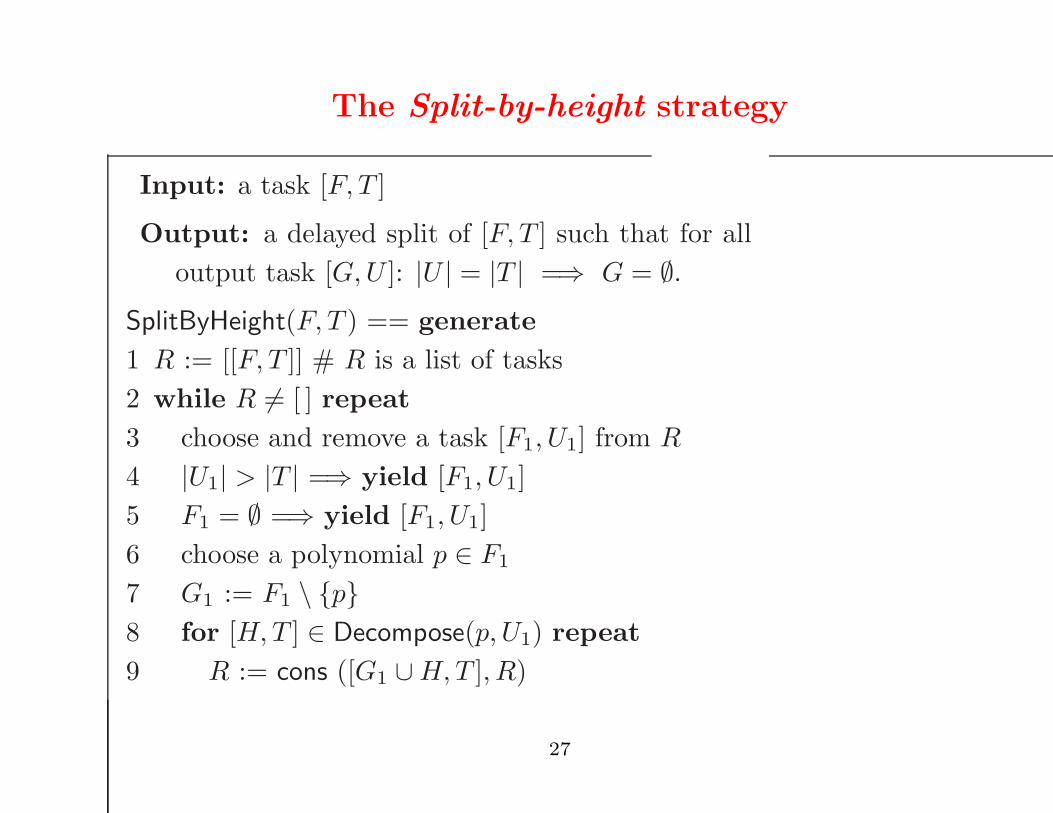
The Split-by-height strategy
Input: a task [F, T ]
Output: a delayed split of [F, T ] such that for all
output task [G, U ]: |U | = |T | =⇒ G = ∅.
SplitByHeight(F, T ) == generate
1 R := [[F, T ]] # R is a list of tasks
2 while R 6= [ ] repeat
3 choose and remove a task [F1, U1] from R
4 |U1| > |T | =⇒ yield [F1, U1]
5 F1 = ∅ =⇒ yield [F1, U1]
6 choose a polynomial p ∈ F1
7 G1 := F1 \ {p}
8 for [H, T ] ∈ Decompose(p, U1) repeat
9 R := cons ([G1 ∪ H, T ], R)
27

A new Triangularize(F, T ) based on SplitByHeight
Input: a task [F, T ]
Output: regular chains T1, . . . , Te solving
[F, T ].
Triangularize(F, T ) == generate
1 R := [[F, T ]] # R is a list of tasks
2 while R 6= [ ] repeat
3 choose and remove [F1, U1] ∈ R with max priority
4 F1 = ∅ =⇒ yield U1
5 for [H, T ] ∈ SplitByHeight(F1, U1) repeat
6 R := cons ([H, T ], R)
7 sort R by decreasing priority
28

Challenges in the implementation
• Encoding complex mathematical objects and sophisticated algorithms.
• Handling dynamic process creation and management (MPI is not
sufficient).
• Scheduling of highly irregular tasks.
• Managing huge intermediate data (with coefficient swell).
• Handling synchronization.
29

Preliminary implementation: Environment
• We use the Aldor programming language:
- designed to express the structures and algorithms in computer algebra,
- which provides a two-level object model of categories and domains,
- which provides interoperability with other languages, such as C, for
high-performance computing.
• We use the BasicMath library (100,000 lines) in Aldor which provides
a sequential implementation of the Triade algorithm.
• We targeted multi-processed parallelism on SMPs.
• Unfortunately, there was no available support in Aldor for our needs.
30

Communication and synchronization
• We have two functional modules, which are stand-alone executable:
Manager and Worker.
• A primer run() in Aldor allows us to launch independent processes
from the Manager.
• We rely on shared memory segments: we have developed a
SharedMemorySegment domain in Aldor.
• Multivariate polynomials are transfered as primitive array of machine
integers via Kronecker substitution.
• Synchronization for data communication between Manager and Worker’s
is controlled by a mailbox protocol.
task_i result_i
Manager
Worker
result_tag_i
write
write
read/freewrite
read/free
read/free
31

Experimentation
• Machine: S¯ilky in Canada’s Shared Hierarchical Academic Research
Computing Network (SHARCNET), SGI Altix 3700 Bx2, 128
Itanium2 Processors (1.6GHz), 64-bit, 256 GB memory, 6 MB cache,
SUSE Linux Enterprise Server 10 (ia64).
• Tests on 7 well-known problems:
– Sequential runs with and without regularized initials
– Parallel with Task Pool Dimension and Rank Guided
Scheduling (TPDRG) in Triangularize, using 3 to 21 processors.
– Parallel with Greedy Scheduling in Triangularize, using the
number of processors
∗ giving the best TPDRG time,
∗ giving the best TPDRG time + 2 processors.
– CPU time in read and write for data communication.
32

Recall: features of the testing problem
Sys Name n d p Degrees
1 eco6 6 3 105761 [1,1,2,4,4,4]
2 eco7 7 3 387799 [1,1,1,1,4,2,
4,4,4,4,4,2]
3 CassouNogues2 4 6 155317 [8]
4 CassouNogues 4 8 513899 [8,8]
5 Nooburg4 4 3 7703 [18,6,6,3,3,4,4,4,4,2,2,2,
2,2,2,2,2,1,1,1,1,1]
6 UteshevBikker 4 3 7841 [1,1,1,1,2,30]
7 Cohn2 4 6 188261 [3,5,2,1,2,1,1,16,12,10,8,8,
4,6,4,4,4,4,2,1,1,1,1,1,1,1,
1,1,1,1,1,1,1]
33
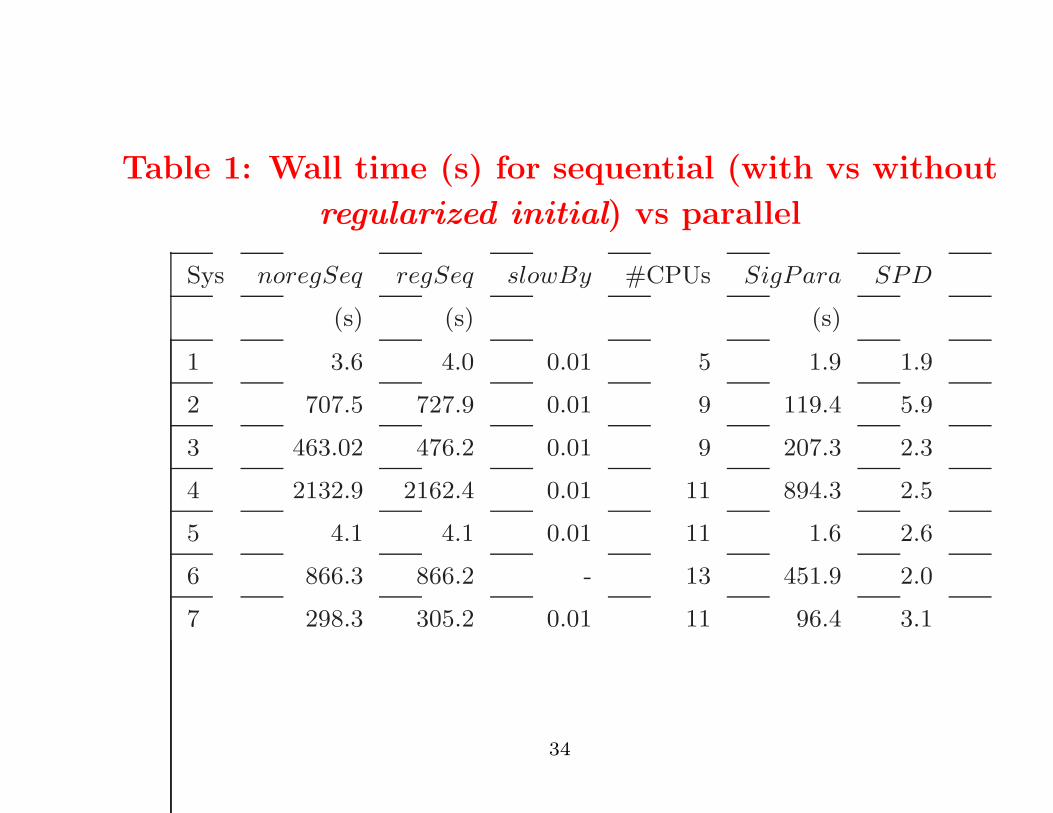
Table 1: Wall time (s) for sequential (with vs without
regularized initial) vs parallel
Sys noregSeq regSeq slowBy #CPUs SigPara SPD
(s) (s) (s)
1 3.6 4.0 0.01 5 1.9 1.9
2 707.5 727.9 0.01 9 119.4 5.9
3 463.02 476.2 0.01 9 207.3 2.3
4 2132.9 2162.4 0.01 11 894.3 2.5
5 4.1 4.1 0.01 11 1.6 2.6
6 866.3 866.2 - 13 451.9 2.0
7 298.3 305.2 0.01 11 96.4 3.1
34

Table 2: Parallel timing (s) vs #processor
#CPUs Sys 1 Sys 2 Sys 3 Sys 4 Sys 5 Sys 6 Sys 7
3 3.1 355.1 278.7 1401.4 2.1 622.9 105.0
5 1.9 225.3 214.2 1004.7 2.1 481.7 98.4
7 1.9 142.7 209.2 939.4 1.9 470.2 97.2
9 1.9 119.4 207.3 905.2 1.8 455.2 96.7
11 2.0 119.5 207.1 894.3 1.6 453.1 96.4
13 - 119.1 206.4 874.5 1.6 451.9 96.4
17 - 120.1 211.7 865.5 1.6 451.6 96.2
21 - 119.2 - 852.5 - 451.3 96.5
35

Table 3: Speedup(s) vs #processor
#CPUs Sys 1 Sys 2 Sys 3 Sys 4 Sys 5 Sys 6 Sys 7
3 1.15 1.99 1.66 1.52 1.95 1.39 2.84
5 1.87 3.14 2.16 2.12 1.95 1.80 3.03
7 1.89 4.96 2.21 2.27 2.15 1.84 3.07
9 1.89 5.92 2.23 2.36 2.31 1.90 3.09
11 1.86 5.92 2.24 2.39 2.51 1.91 3.10
13 - 5.94 2.24 2.44 2.55 1.92 3.09
36

Speedup vs number of processors
0
2
4
6
8
10
12
0 2 4 6 8 10 12
Sp
ee
du
p
Number of Processors
Linear Speedupeco6eco7
Caou-Nogue-2Caou-Nogue
Cohn-2Nooburg-4
Uteshev-Bikker
37
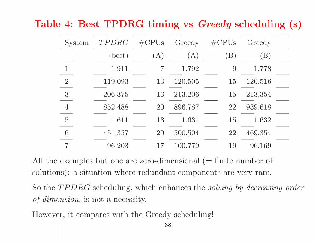
Table 4: Best TPDRG timing vs Greedy scheduling (s)
System TPDRG #CPUs Greedy #CPUs Greedy
(best) (A) (A) (B) (B)
1 1.911 7 1.792 9 1.778
2 119.093 13 120.505 15 120.516
3 206.375 13 213.206 15 213.354
4 852.488 20 896.787 22 939.618
5 1.611 13 1.631 15 1.632
6 451.357 20 500.504 22 469.354
7 96.203 17 100.779 19 96.169
All the examples but one are zero-dimensional (= finite number of
solutions): a situation where redundant components are very rare.
So the TPDRG scheduling, which enhances the solving by decreasing order
of dimension, is not a necessity.
However, it compares with the Greedy scheduling!38

Table 5: CPU time in read and write for data
communication vs workers’ total
System DataSize Read Write Workers Read + Write
(#integer) (ms) (ms) (ms) vs Total
1 7717 80 56 1031 13.2%
2 56689 383 172 174329 0.3%
3 112802 4394 301 125830 3.7%
4 430217 33760 426 585112 5.8%
5 13307 123 55 1121 15.9%
6 254145 9773 386 233582 4.4%
7 77426 819 317 31858 3.6%
39

Conclusions
• By using modular methods, we have created opportunities for coarse
grained component-level parallel solving of polynomial systems in Q[X ]
• To exploit these opportunities, we have transformed the Triade algorithm.
• We have strengthened its notion of a task and replaced the operation
Decompose by SplitByHeight in order to
- reduce the depth of the task tree,
- create more work at each node,
- be able to estimate the cost of each task within each parallel step.
• We have realized a preliminary implementation in Aldor using
multi-processed parallelism with shared memory segment for
data-communication.
40

Toward Efficient Multi-level Parallelization
• We aim at developing a model for threads in Aldor to support
parallelism for symbolic computations targeting SMP and multi-cores.
– in particular, parametric types, such as polynomial data types,
shall be properly treated.
• We aim at investigating multi-level parallel algorithms for triangular
decompositions of polynomial systems.
– coarse grained level for tasks to compute geometric of the solution
sets.
– medium/fine grained level for polynomial arithmetic such as
multiplication, GCD/resultant, and factorization.
– hence, to increase speed-up.
41
Propaganda
ISSAC 07
PASCO 07 SNC 07
ACA 07
London, July 27−28 London, July 25 −27
Waterloo, July 29 −1
Detroit, Aug 3−6
42