complexity of optimization problems. optimal methods...
TRANSCRIPT
1
Complexity of optimization problems.
Optimal methods for convex optimization problems
Gasnikov Alexander (MIPT, IITP RAS)
Двенадцатая Международная Школа-семинар «Проблемы оптимизации сложных систем»
Новосибирск, Академгородок, ИВМиМГ СО РАН
12-16 декабря 2016 г.

2
Complexity theory of convex optimization
was built in 1976–1979 mainly in works of
Arkadi Nemirovski
3
Main books:
Nemirovski A. Efficient methods in convex programming. Technion, 1995.
http://www2.isye.gatech.edu/~nemirovs/Lec_EMCO.pdf
Nesterov Yu. Introduction Lectures on Convex Optimization. A Basic Course. Applied Optimiza-
tion. – Springer, 2004.
Nemirovski A. Lectures on modern convex optimization analysis, algorithms, and engineering
applications. – Philadelphia: SIAM, 2013.
Bubeck S. Convex optimization: algorithms and complexity // In Foundations and Trends in Ma-
chine Learning. – 2015. – V. 8. – no. 3-4. – P. 231–357.
Guzman C., Nemirovski A. On lower complexity bounds for large-scale smooth convex optimiza-
tion // Journal of Complexity. – 2015. – V. 31. – P. 1–14.
Gasnikov A., Nesterov Yu. Universal fast gradient method for stochastic composit optimization
problems // e-print, 2016. https://arxiv.org/ftp/arxiv/papers/1604/1604.05275.pdf
4
Structure of Lectures
Pessimistic lower bound for non convex problems
Resisting oracle
Optimal estimation for convex optimization problems
Lower complexity bounds
Optimal and not optimal methods
Mirror Descent
Gradient Descent
Similar Triangles Method (Fast Gradient Method)
Open gap problem of A. Nemirovski
Structural optimization (looking into the Black Box)
Conditional problems
Interior Point Method
5
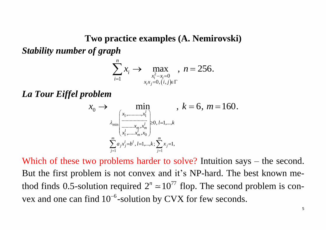
Two practice examples (A. Nemirovski)
Stability number of graph
2 01
0, ,
max ,i i
i j
n
ix x
ix x i j
x
256n .
La Tour Eiffel problem
1 1
min
1 0
1 1
0,..........,
...................0, 1,...,
......... ,
,..... ,
, 1,..., ; 1,
min ,l
lm m
l lm
m ml l
j j j
j j
x x
l kx x
x x x
a x b l k x
x
6k , 160m .
Which of these two problems harder to solve? Intuition says – the second.
But the first problem is not convex and it’s NP-hard. The best known me-
thod finds 0.5-solution required 772 10n flop. The second problem is con-
vex and one can find 610 -solution by CVX for few seconds.
6
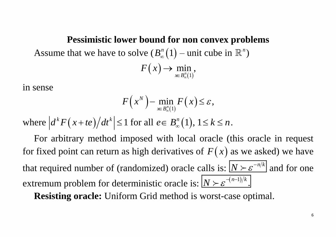
Pessimistic lower bound for non convex problems
Assume that we have to solve ( 1nB – unit cube in n )
1
min ,nx B
F x
in sense
1
min ,n
N
x BF x F x
where 1k kd F x te dt for all 1ne B , 1 k n .
For arbitrary method imposed with local oracle (this oracle in request
for fixed point can return as high derivatives of F x as we asked) we have
that required number of (randomized) oracle calls is: n kN and for one
extremum problem for deterministic oracle is:
1.
n kN
Resisting oracle: Uniform Grid method is worst-case optimal.
7
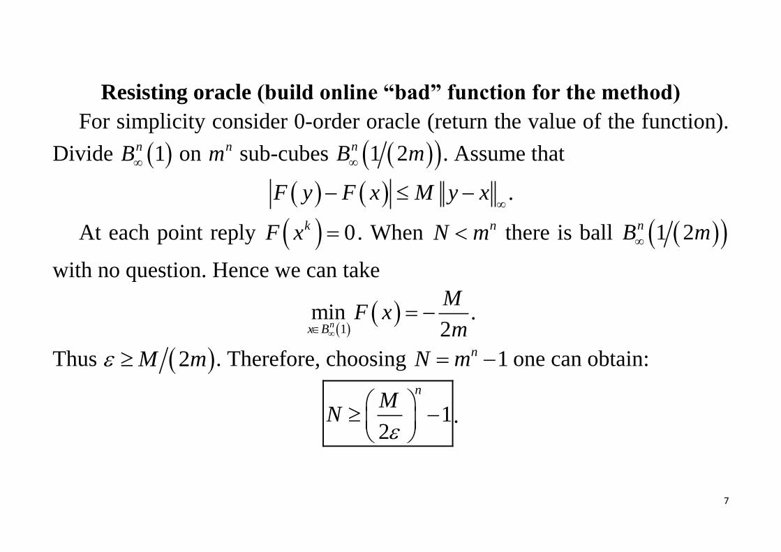
Resisting oracle (build online “bad” function for the method)
For simplicity consider 0-order oracle (return the value of the function).
Divide 1nB on nm sub-cubes 1 2nB m . Assume that
F y F x M y x
.
At each point reply 0kF x . When nN m there is ball 1 2nB m
with no question. Hence we can take
1min
2nx B
MF x
m .
Thus 2M m . Therefore, choosing 1nN m one can obtain:
12
nM
N
.
8
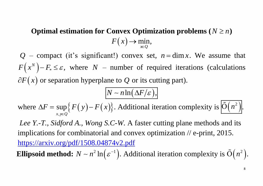
Optimal estimation for Convex Optimization problems (N n )
min,x Q
F x
Q – compact (it’s significant!) convex set, dimn x . We assume that
* ,NF x F where N – number of required iterations (calculations
F x or separation hyperplane to Q or its cutting part).
ln ,N n F
where ,
supx y Q
F F y F x
. Additional iteration complexity is 2n .
Lee Y.-T., Sidford A., Wong S.C-W. A faster cutting plane methods and its
implications for combinatorial and convex optimization // e-print, 2015.
https://arxiv.org/pdf/1508.04874v2.pdf
Ellipsoid method: 2 1ln .N n Additional iteration complexity is 2n .
9
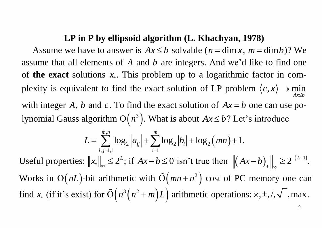
LP in P by ellipsoid algorithm (L. Khachyan, 1978)
Assume we have to answer is Ax b solvable ( dimn x , dimm b )? We
assume that all elements of A and b are integers. And we’d like to find one
of the exact solutions *x . This problem up to a logarithmic factor in com-
plexity is equivalent to find the exact solution of LP problem , minAx b
c x
with integer A, b and c . To find the exact solution of Ax b one can use po-
lynomial Gauss algorithm 3n . What is about Ax b ? Let’s introduce
,
2 2 2
, 1,1 1
log log log 1.m n m
ij i
i j i
L a b mn
Useful properties: * 2Lx
; if 0Ax b isn’t true then 1
2 .L
Ax b
Works in nL -bit arithmetic with 2mn n cost of PC memory one can
find *x (if it’s exist) for 3 2n n m L arithmetic operations: , , /, ,max .
10
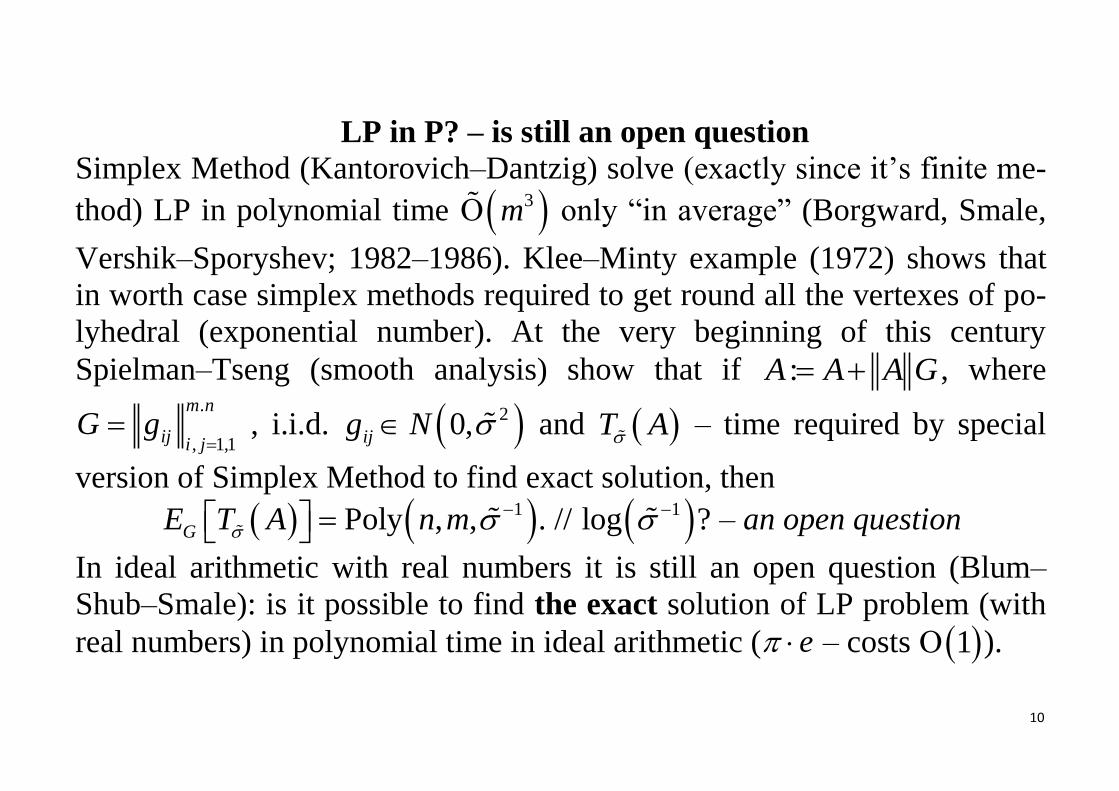
LP in P? – is still an open question
Simplex Method (Kantorovich–Dantzig) solve (exactly since it’s finite me-
thod) LP in polynomial time 3m only “in average” (Borgward, Smale,
Vershik–Sporyshev; 1982–1986). Klee–Minty example (1972) shows that
in worth case simplex methods required to get round all the vertexes of po-
lyhedral (exponential number). At the very beginning of this century
Spielman–Tseng (smooth analysis) show that if :A A A G , where .
, 1,1
m n
ij i jG g
, i.i.d. 20,ijg N and T A – time required by special
version of Simplex Method to find exact solution, then
1Poly , ,GE T A n m . // 1log ? – an open question
In ideal arithmetic with real numbers it is still an open question (Blum–
Shub–Smale): is it possible to find the exact solution of LP problem (with
real numbers) in polynomial time in ideal arithmetic ( e – costs 1 ).

11
Optimal estimations for Convex Optimization problems (N n )
min.x Q
F x
We assume that
* .NF x F
N – number of required iterations (calculations of F x and F x ).
R – “distance” between starting point and nearest solution.
N F y F x M y x *
F y F x L y x
F x convex 2 2
2
M R
2LR
F x -strongly convex 2M
2
lnL R
N
If norm is non euclidian then the last row is true up to ln n -factor.

12
Lower complexity bound. Non smooth case (N n )
Let’s introduce
2 2nQ B R , 2
21max
2N i
i NF x M x x
,
M
R N ,
1 0 0Lin ,...,k kx x f x f x . // method
Solving the problem
2 min2
NM
we get * R N , 2 2 2
* *2x N R , * minN N
x QF F x MR N
. If
0 0x then after N iteration we can keep 0N
ix for i N . So we have
21 * *
1 1 1 , .2 11
N
N N N
MR MF x F F
NN

13
Lower complexity bound. Smooth case
Let’s introduce (2 1N n ): 0 0x , 0Lin ,...,k kx f x f x ,
2 1
22 2
1 1 2 1 1
18 4
N
N i i N
i
L LF x x x x x x
,
Then
21
** 2
21
3min
32 1
i
N Ni N
x xLF x F
N
.
Let’s introduce L
2 22
1 1 1 21
12
8 2i i
i
F x x x x x x
Then 2 1
21
* * 2
1
2 1
N
NF x F x x
(with arbitrary
1N ).
14
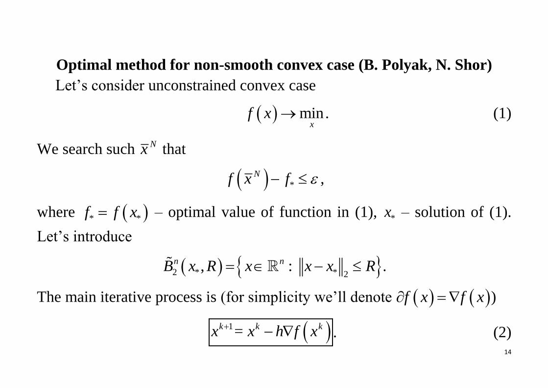
Optimal method for non-smooth convex case (B. Polyak, N. Shor)
Let’s consider unconstrained convex case
minx
f x . (1)
We search such Nx that
*
Nf x f ,
where * *f f x – optimal value of function in (1), *x – solution of (1).
Let’s introduce
2 * * 2, :n nB x R x x x R .
The main iterative process is (for simplicity we’ll denote f x f x )
1=k k kx x h f x . (2)
15
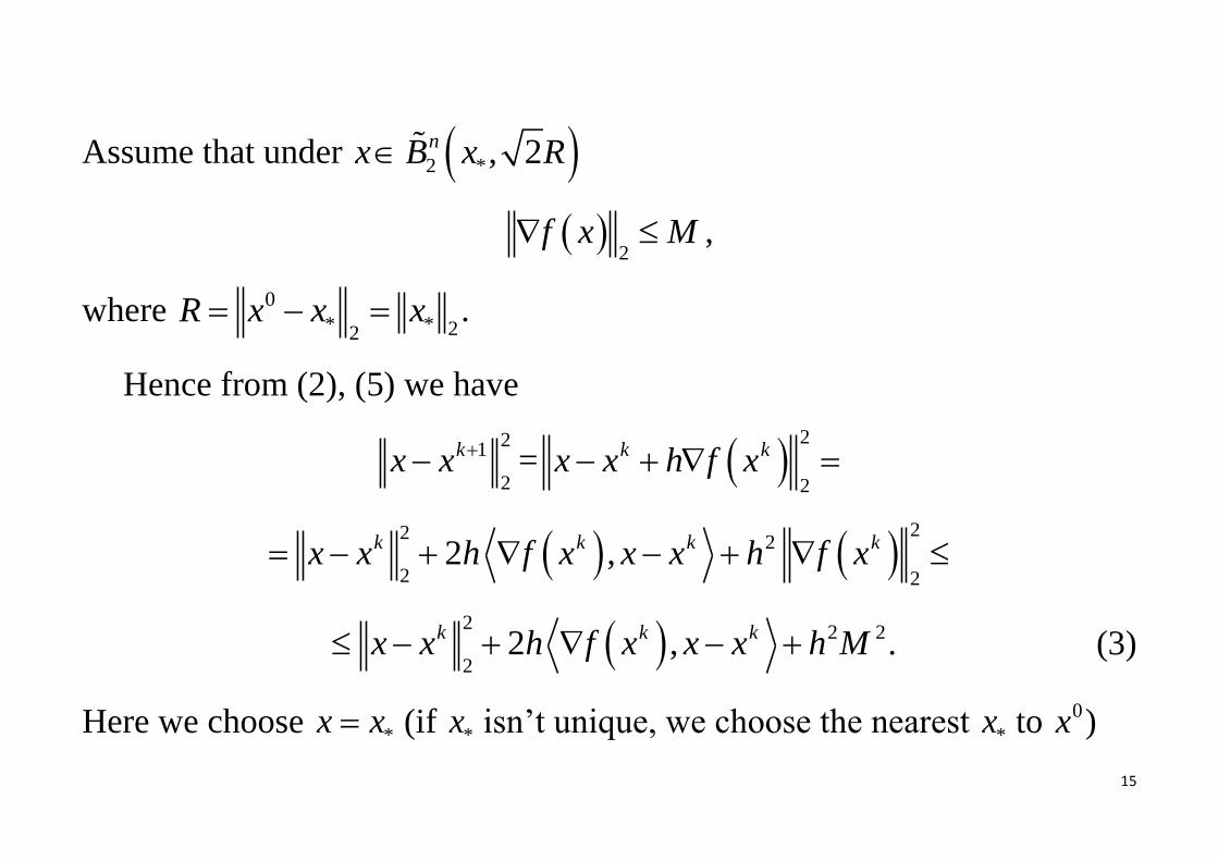
Assume that under 2 *, 2nx B x R
2
f x M ,
where 0
* * 22R x x x .
Hence from (2), (5) we have
22
1
2 2=k k kx x x x h f x
22
2
2 22 ,k k k kx x h f x x x h f x
2
2 2
22 ,k k kx x h f x x x h M . (3)
Here we choose *x x (if *x isn’t unique, we choose the nearest *x to 0x )

16
1 1 1
* * *
0 0 0
1 1 1,
N N Nk k k k
k k k
f x f f x f x f x x xN N N
21
2 21
* *2 20
1
2 2
Nk k
k
hMx x x x
hN
2
2 20
* *2 2
1
2 2
N hMx x x x
hN .
If R
hM N
, 1
0
1 NN k
k
x xN
,
then
*
N MRf x f
N . (4)
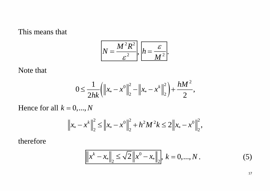
17
This means that
2 2
2
M RN
,
2h
M
.
Note that
2
2 20
* *2 2
10
2 2
k hMx x x x
hk ,
Hence for all 0,...,k N
2 2 20 2 2 0
* * *2 2 22kx x x x h M k x x ,
therefore
0
* *2 22kx x x x , 0,...,k N . (5)
18
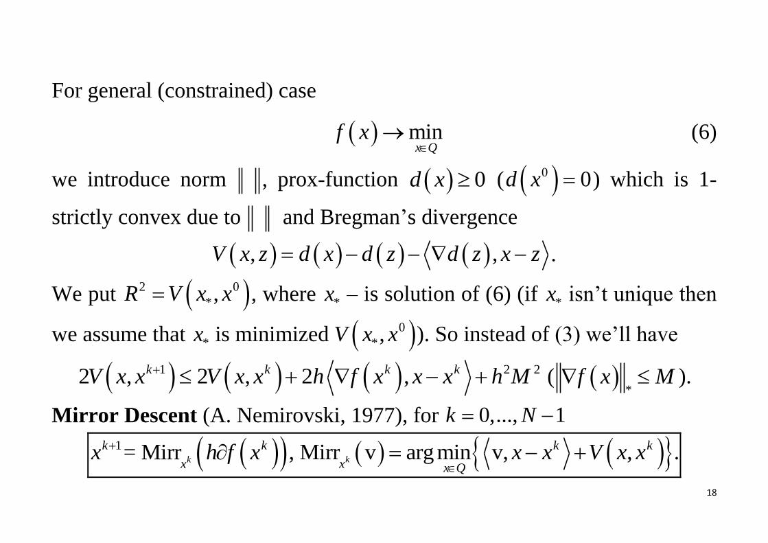
For general (constrained) case
minx Q
f x
(6)
we introduce norm , prox-function 0d x ( 0 0d x ) which is 1-
strictly convex due to and Bregman’s divergence
, ,V x z d x d z d z x z .
We put 2 0
*,R V x x , where *x – is solution of (6) (if *x isn’t unique then
we assume that *x is minimized 0
*,V x x ). So instead of (3) we’ll have
1 2 22 , 2 , 2 ,k k k kV x x V x x h f x x x h M ( *
f x M ).
Mirror Descent (A. Nemirovski, 1977), for 0,..., 1k N
1= Mirr ,k
k k
xx h f x Mirr v arg min v, , .k
k k
x x Qx x V x x
19
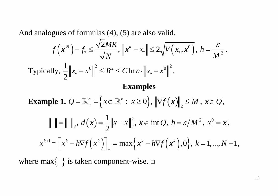
And analogues of formulas (4), (5) are also valid.
*
2N MRf x f
N , 0
* *2 ,kx x V x x , 2
hM
.
Typically, 2 2
0 2 0
* *
1ln
2x x R C n x x .
Examples
Example 1. : 0n nQ x x , 2
f x M , x Q ,
2 ,
2
2
1
2d x x x , intx Q , 2h M , 0x x ,
1= max ,0k k k k kx x h f x x h f x
, 1,..., 1k N ,
where max is taken component-wise. □
20
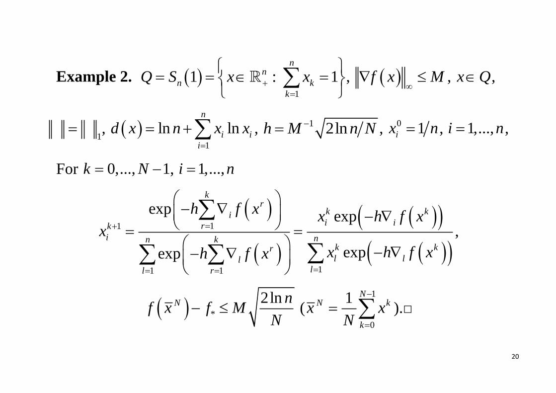
Example 2. 1
1 : 1n
n
n k
k
Q S x x
, f x M
, x Q ,
1 ,
1
ln lnn
i i
i
d x n x x
, 1 2lnh M n N , 0 1ix n , 1,...,i n ,
For 0,..., 1k N , 1,...,i n
11
11 1
expexp
expexp
kr
k kii irk
i nn kk krl ll
ll r
h f xx h f x
x
x h f xh f x
,
*
2lnN nf x f M
N (
1
0
1 NN k
k
x xN
).□
21
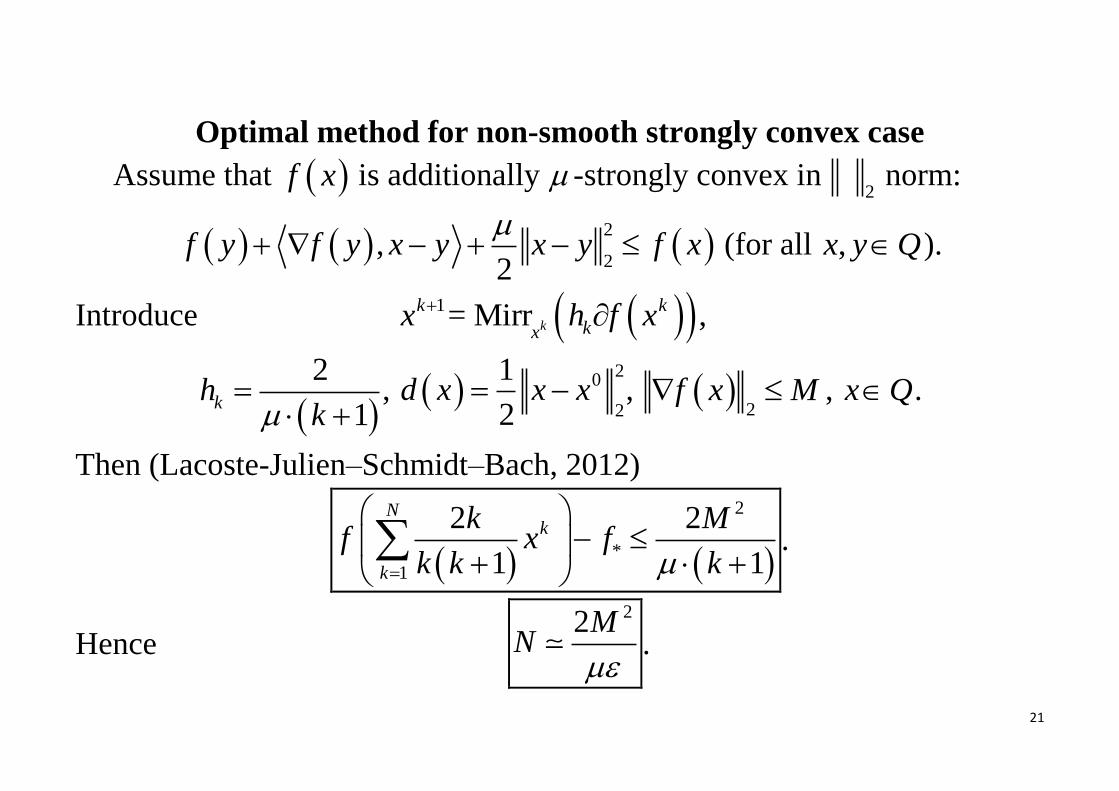
Optimal method for non-smooth strongly convex case
Assume that f x is additionally -strongly convex in 2 norm:
2
2,
2f y f y x y x y f x
(for all ,x y Q ).
Introduce 1= Mirr ,k
k k
kxx h f x
2
1kh
k
,
20
2
1
2d x x x ,
2f x M , x Q .
Then (Lacoste-Julien–Schmidt–Bach, 2012)
2
*
1
2 2
1 1
Nk
k
k Mf x f
k k k
.
Hence
22MN
.
22
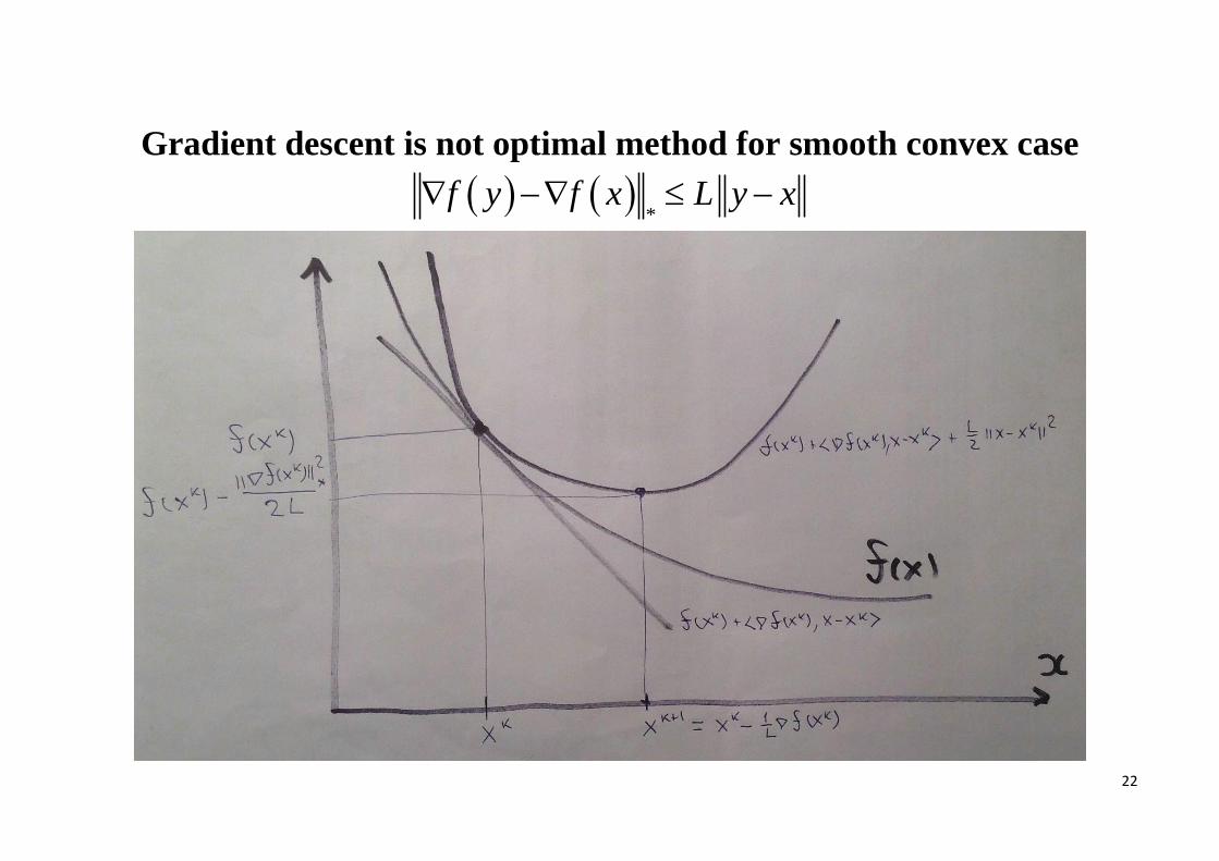
Gradient descent is not optimal method for smooth convex case
*
f y f x L y x

23
2
1 arg min , ,2
k k k k k
x Q
Lx f x f x x x x x
2
*
2,N LR
f x fN
0
2
*,max .
x Q f x f xR x x
In Euclidian case (2-norm) one can simplify
1 1,k k k
Qx x f xL
2
*
2,N LR
f x fN
0
* 2.R x x
If nQ one has
1 1.k k kx x f x
L
Unfortunately, convergence of simple gradient descent isn’t optimal!
24
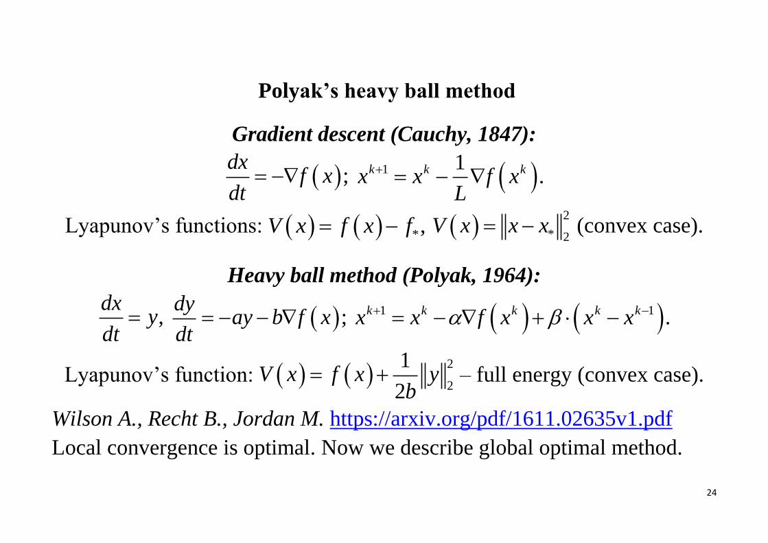
Polyak’s heavy ball method
Gradient descent (Cauchy, 1847):
;dx
f xdt
1 1.k k kx x f x
L
Lyapunov’s functions: *,V x f x f 2
* 2V x x x (convex case).
Heavy ball method (Polyak, 1964):
,dx
ydt
;dy
ay b f xdt
1 1 .k k k k kx x f x x x
Lyapunov’s function: 2
2
1
2V x f x y
b – full energy (convex case).
Wilson A., Recht B., Jordan M. https://arxiv.org/pdf/1611.02635v1.pdf
Local convergence is optimal. Now we describe global optimal method.

25
Optimal method for smooth convex case Estimation functions technique (Yu. Nesterov)
0 0,d y 0,d x
, , ,V x z d x d z d z x z
0 0 0 0
0 0, ,x V x y f y f y x y
,
1 1 1
1 1 ,k k k
k k kx x f y f y x y
0 0
0arg minx Q
x u x
, 0
k
k i
i
A
, 1
0 L , 2
k kA L ,
2
1 2
1 1
2 4k k
L L ,
2
1
4k
kA
L
, 0,1,2,...k
26
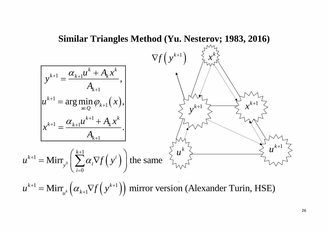
Similar Triangles Method (Yu. Nesterov; 1983, 2016)
1 1
1
1
1
11 1
1
,
arg min ,
.
k kk k k
k
k
kx Q
k kk k k
k
u A xy
A
u x
u A xx
A
0
11
0
Mirr the samek
k i
iyi
u f y
1 1
1Mirr mirror version (Alexander Turin, HSE)k
k k
kuu f y
kx
1ku ku
1ky
1kx
1kf y
27
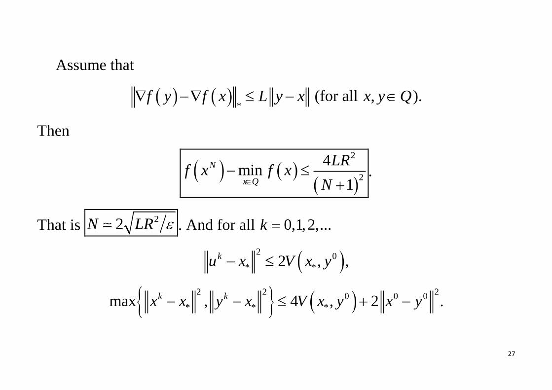
Assume that
*
f y f x L y x (for all ,x y Q ).
Then
2
2
4min
1
N
x Q
LRf x f x
N
.
That is 22N LR . And for all 0,1,2,...k
2
0
* *2 ,ku x V x y ,
2 2 2
0 0 0
* * *max , 4 , 2k kx x y x V x y x y .
28
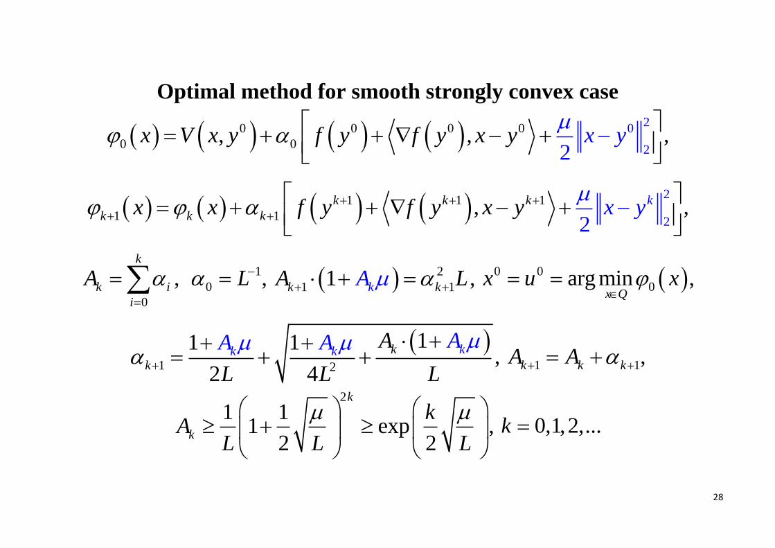
Optimal method for smooth strongly convex case
0 0 0 0 0
0 0
2
2, ,
2x V x y f y f y x x yy
,
1 1 1
1
2
212
, kk k k
k k kx x f y x yf y x y
,
0
k
k i
i
A
, 1
0 L , 2
1 11 kk k LAA , 0 0
0arg minx Q
x u x
,
1 2
11 1
2 4
kk kkk
AA A A
L L L
, 1 1k k kA A ,
2
1 11 exp
2 2
k
k
kA
L L L
, 0,1,2,...k
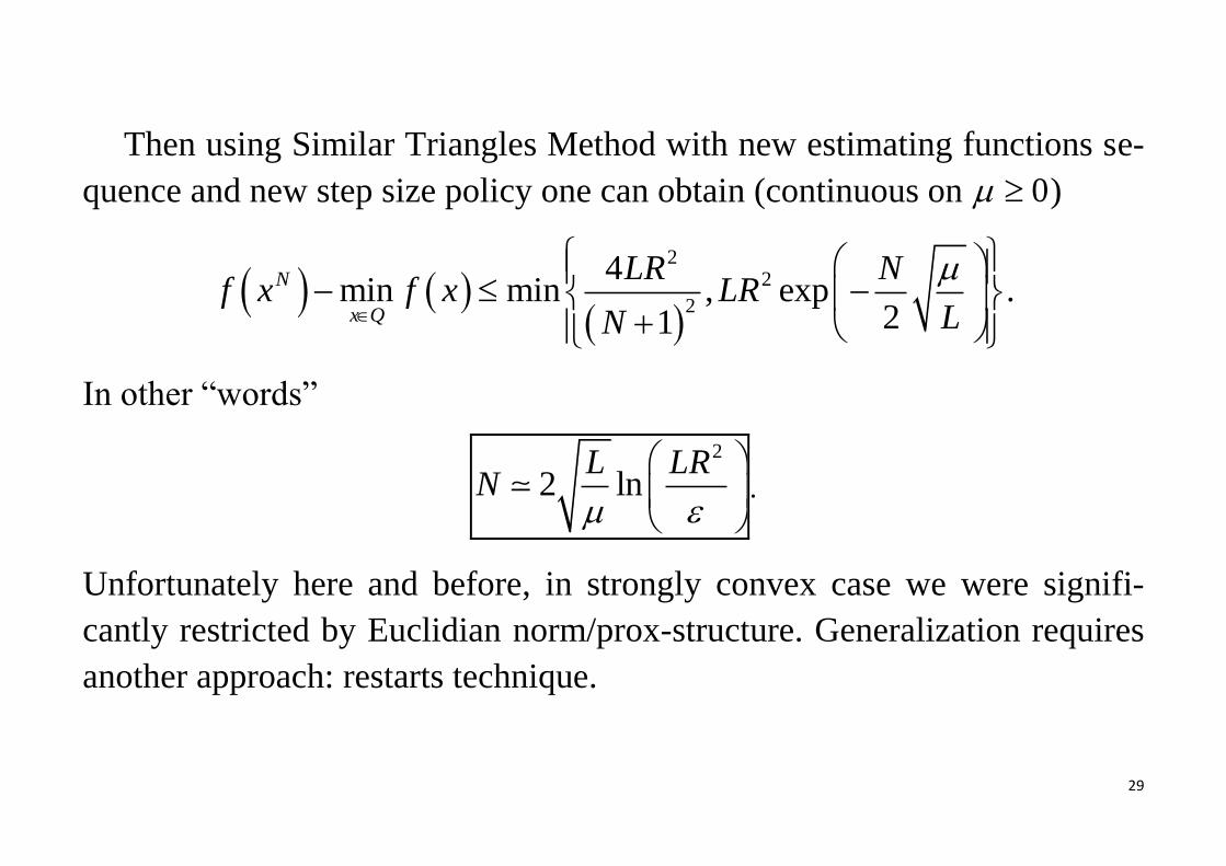
29
Then using Similar Triangles Method with new estimating functions se-
quence and new step size policy one can obtain (continuous on 0 )
22
2
4min min , exp
21
N
x Q
LR Nf x f x LR
LN
.
In other “words”
2
2 lnL LR
N
.
Unfortunately here and before, in strongly convex case we were signifi-
cantly restricted by Euclidian norm/prox-structure. Generalization requires
another approach: restarts technique.
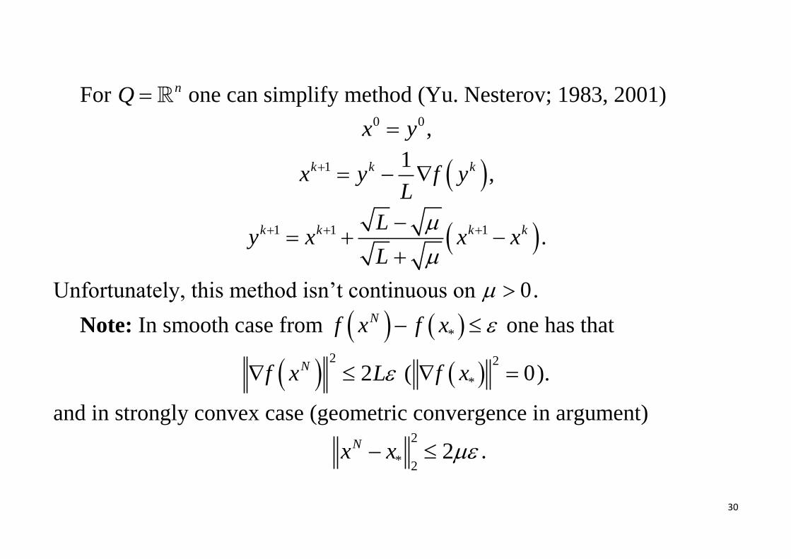
30
For nQ one can simplify method (Yu. Nesterov; 1983, 2001) 0 0x y ,
1 1k k kx y f yL
,
1 1 1k k k kLy x x x
L
.
Unfortunately, this method isn’t continuous on 0 .
Note: In smooth case from *
Nf x f x one has that
2
2Nf x L ( 2
* 0f x ).
and in strongly convex case (geometric convergence in argument) 2
* 22Nx x .

31
Open gap problem (A. Nemirovski, 2015)
Assume that 1
nQ B R (ball in n of radius R in 1-norm),
2 22f y f x L y x .
Then for N n and arbitrary method with local first order oracle
2
1 2* 3
N C L Rf x f
N .
When 1 1f y f x L y x
Similar Triangles Methods takes us
2
2 1* 2
N C L Rf x f
N ,
where 2 1 2L n L L . Unfortunately, we can’t say that there is no gap be-
tween lower and upper bounds.

32
Optimality
Meanwhile, for the most interesting convex sets Q there exists such a norm
and appropriate prox-structure d x that Mirror Descent and Similar
Triangles Method (and theirs restart-strongly convex variants) lead (up to a
logarithmic factor) to unimprovable estimations, collected in the table be-
low (we assume that all parameters M , L , R , we choose correspond to
the norm – this isn’t true for A. Nemirovski example):
N F y F x M y x *
F y F x L y x
F x convex 2 2
2
M R
2LR
F x -strongly convex 2M
2
lnL R
If norm is non euclidian then the last row is true up to ln n -factor.

33
How to choose norm and prox function?
Arkadi Nemirovski, 1979
2log 11
2log 1 2log
na
n n
1n
pQ B 1 p a 2a p 2 p
a
p
2
d x
21
2 1 ad x x
a
21
2 1 pd x x
p
2
2
1
2x
2R logn 11p
1
34
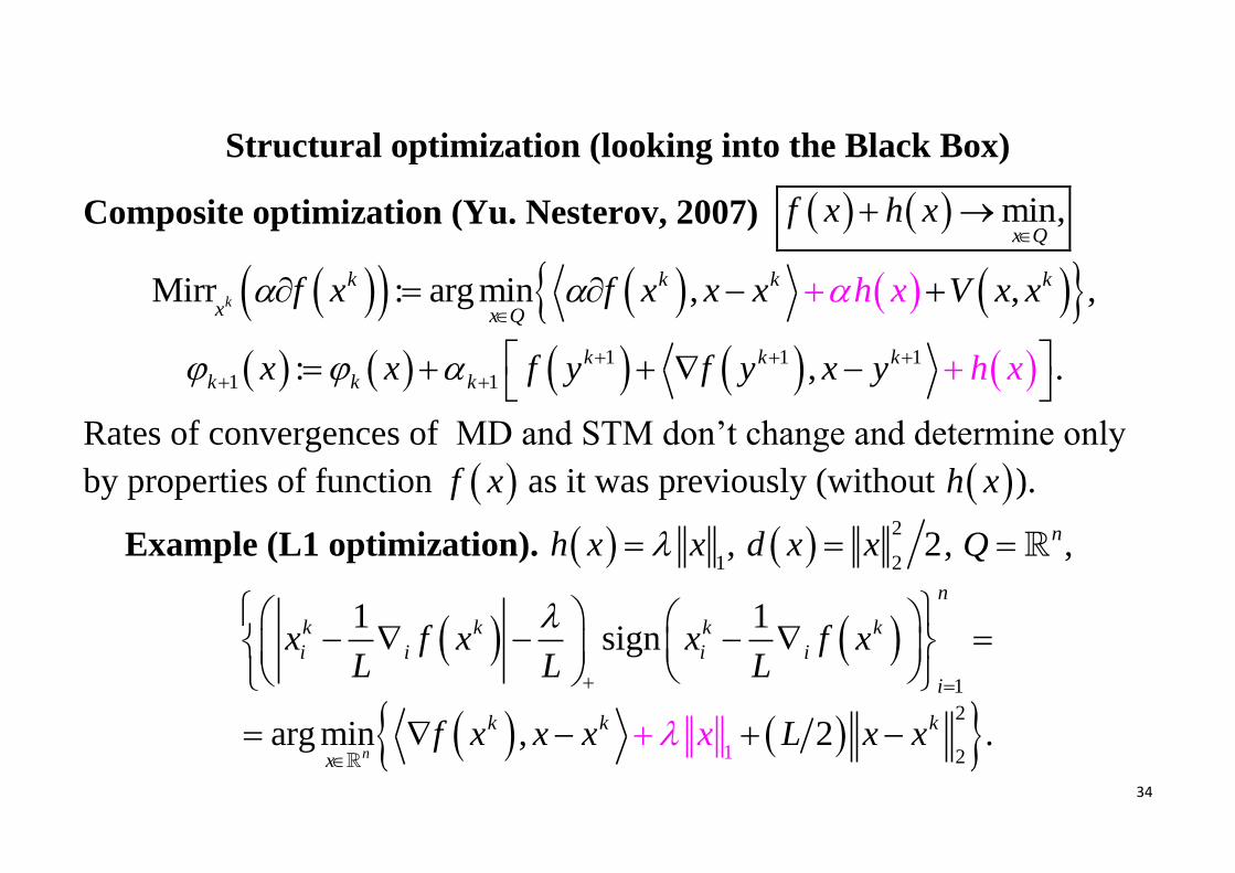
Structural optimization (looking into the Black Box)
Composite optimization (Yu. Nesterov, 2007) min,x Q
f x h x
Mirr : arg min , , ,k
k k k k
x x Qf x f x x x h Vx x x
1 1 1
1 1: , .k k k
k k k hx x f y f y x xy
Rates of convergences of MD and STM don’t change and determine only
by properties of function f x as it was previously (without h x ).
Example (L1 optimization). 1
h x x , 2
22d x x , nQ ,
1
1 1sign
n
k k k k
i i i i
i
x f x x f xL L L
21
2
arg min , 2 .n
k k k
xf x x L xxx x

35
Structural optimization (looking into the Black Box)
MinMax problem (idea A. Nemirovski, 1979; Yu. Nesterov, 2004)
1,...,
max min,lx Ql m
F x f x h x
1,...
1
,
1 1 1
1 marg min , ,a .xk k k k k
ku
l ll mQ
u f y f y u y V u uh u
Unfortunately in general this sub-problem isn’t simple enough. But the num-
ber of such iteration of Turins’ variant of STM will be the same (up to a con-
stant) as in the case of previous slide
2
* 2
8,
1
N LRF x F
N
*, , , 1,.., .l lf y f x L y x x y Q l m
One can also generalize this result further:
Lan G. Bundle-level methods uniformly optimal for smooth and non-smooth
convex optimization // Math. program. Ser. A. 2015. V. 149. no. 1. P. 1–45.
36
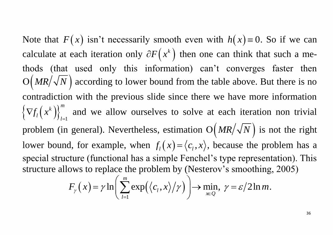
Note that F x isn’t necessarily smooth even with 0h x . So if we can
calculate at each iteration only kF x then one can think that such a me-
thods (that used only this information) can’t converges faster then
MR N according to lower bound from the table above. But there is no
contradiction with the previous slide since there we have more information
1
mk
ll
f x
and we allow ourselves to solve at each iteration non trivial
problem (in general). Nevertheless, estimation MR N is not the right
lower bound, for example, when ,l lf x c x , because the problem has a
special structure (functional has a simple Fenchel’s type representation). This
structure allows to replace the problem by (Nesterov’s smoothing, 2005)
1
ln exp , min,m
lx Q
l
F x c x
2lnm .
37
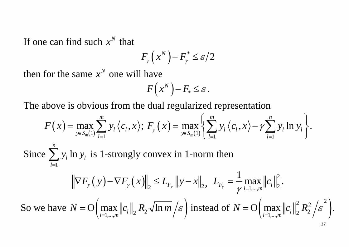
If one can find such Nx that
* 2NF x F
then for the same Nx one will have
*
NF x F .
The above is obvious from the dual regularized representation
1
1
max ,m
m
l ly S
l
F x y c x
; 1
1 1
max , lnm
m n
l l l ly S
l l
F x y c x y y
.
Since 1
lnn
l l
l
y y
is 1-strongly convex in 1-norm then
22 FF y F x L y x
, 2
21,...,
1max .F ll m
L c
So we have 221,...,max lnll m
N c R m
instead of 22 2
221,...,max ll m
N c R
.
38
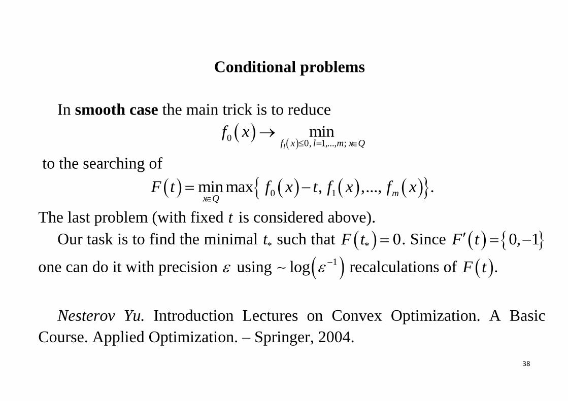
Conditional problems
In smooth case the main trick is to reduce
00, 1,..., ;min
lf x l m x Qf x
to the searching of
0 1min max , ,..., .mx Q
F t f x t f x f x
The last problem (with fixed t is considered above).
Our task is to find the minimal *t such that * 0F t . Since 0, 1F t
one can do it with precision using 1log recalculations of F t .
Nesterov Yu. Introduction Lectures on Convex Optimization. A Basic
Course. Applied Optimization. – Springer, 2004.
39
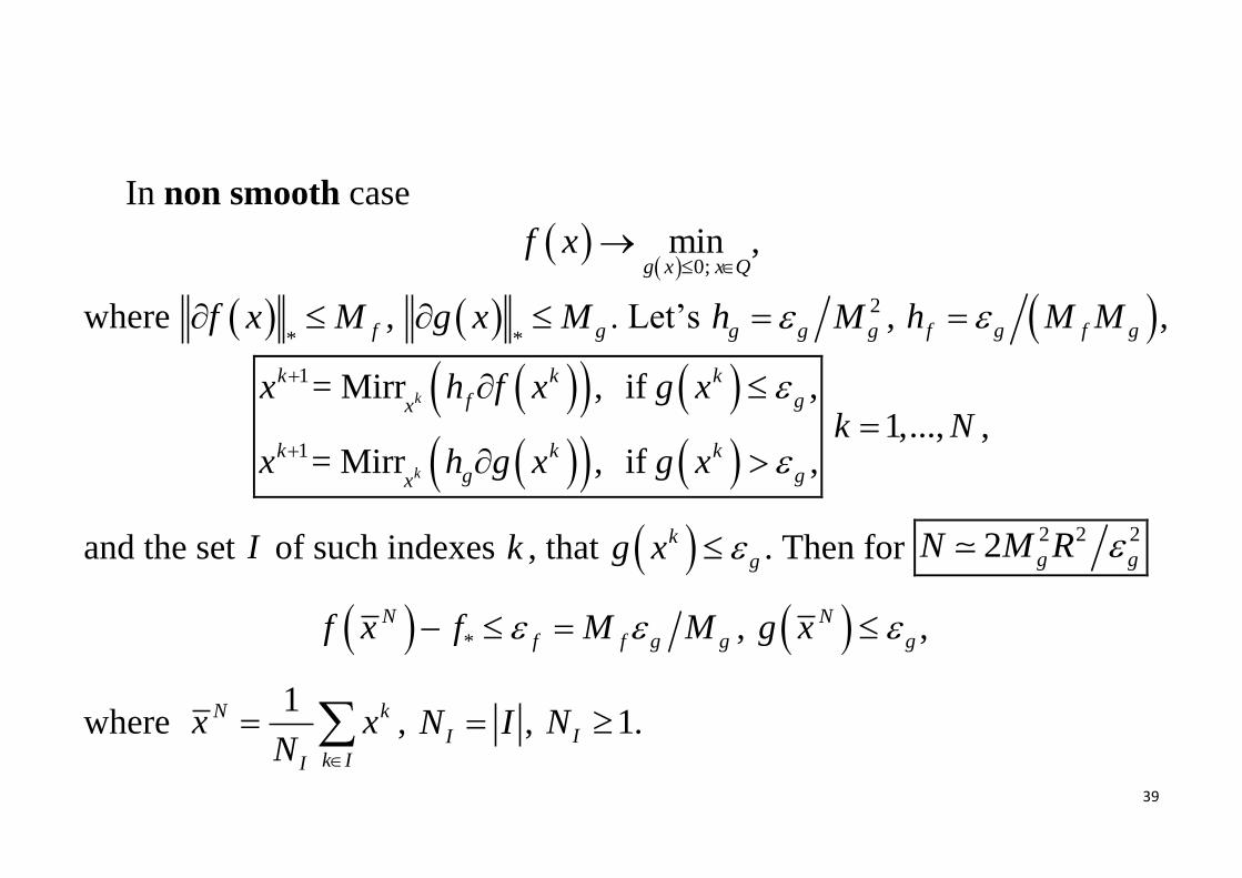
In non smooth case
0;min ,
g x x Qf x
where * ff x M ,
* gg x M . Let’s 2
g g gh M , f g f gh M M ,
1
1
= Mirr , if ,
= Mirr , if ,
k
k
k k k
f gx
k k k
g gx
x h f x g x
x h g x g x
1,...,k N ,
and the set I of such indexes k , that k
gg x . Then for 2 2 22 g gN M R
*
N
f f g gf x f M M , N
gg x ,
where 1N k
k II
x xN
, IN I , 1IN .
40
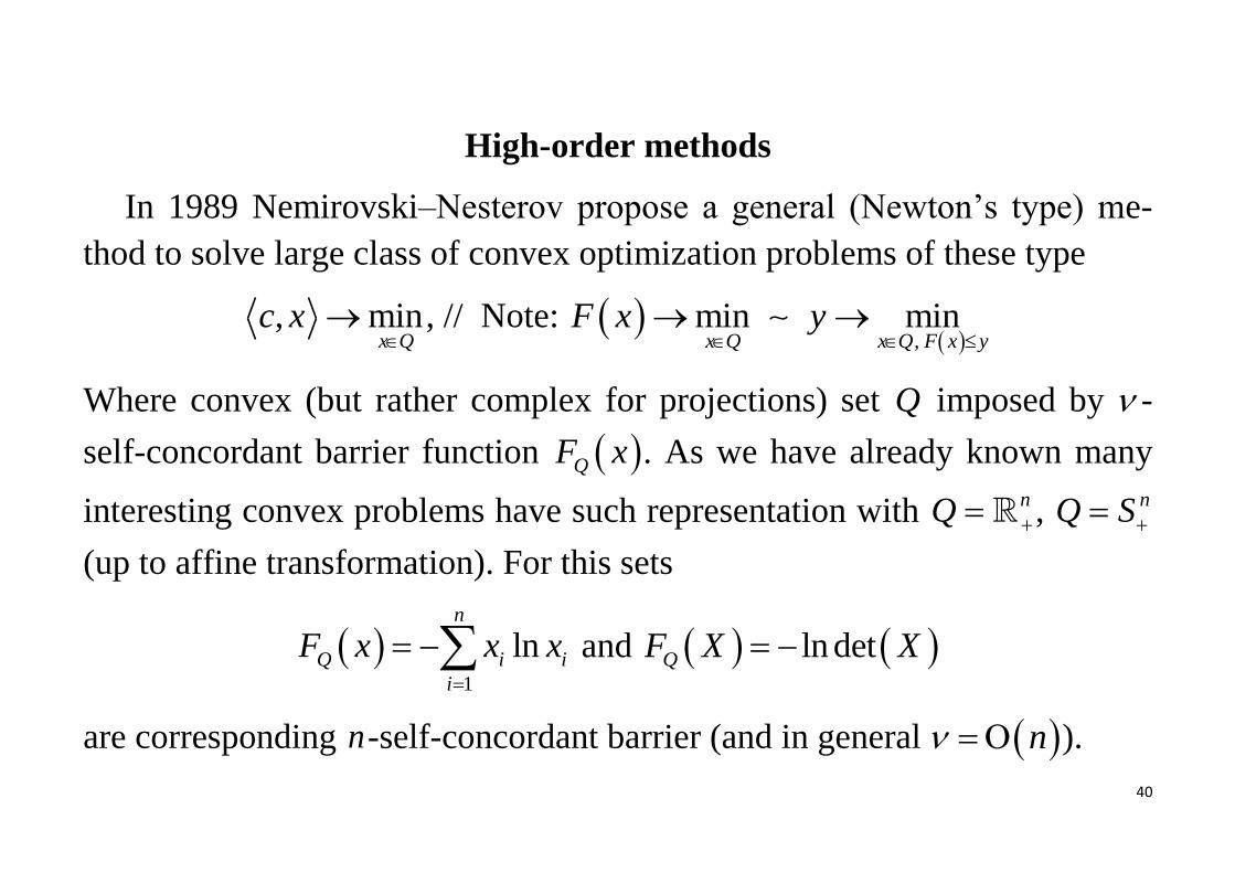
High-order methods
In 1989 Nemirovski–Nesterov propose a general (Newton’s type) me-
thod to solve large class of convex optimization problems of these type
, minx Q
c x
, // Note: ,
min minx Q x Q F x y
F x y
Where convex (but rather complex for projections) set Q imposed by -
self-concordant barrier function QF x . As we have already known many
interesting convex problems have such representation with nQ , nQ S
(up to affine transformation). For this sets
1
lnn
Q i i
i
F x x x
and ln detQF X X
are corresponding n-self-concordant barrier (and in general n ).

41
Interior Point Method (inserted in CVX)
The proposed method looks as follows
1 11
13
k kt t
,
1
1 2 1k k k k k
Q Qx x F x t c F x
.
With proper choose of starting point (these procedure costs log )
described IPM has the following rate of convergence logN .
This estimation is better (since n ) than lower bound 1logn
(we consider here the case N n ). There is no contradiction here, because
of additional assumption about the structure of the problem.
42
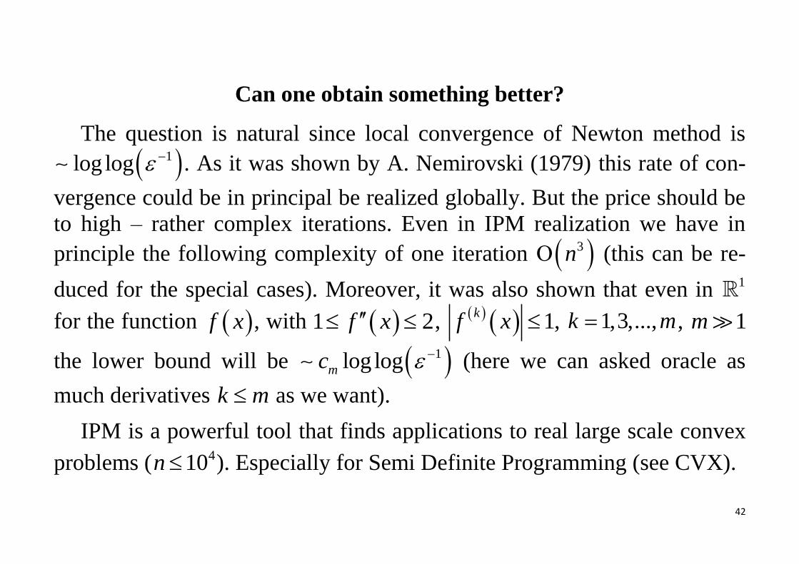
Can one obtain something better?
The question is natural since local convergence of Newton method is
1log log . As it was shown by A. Nemirovski (1979) this rate of con-
vergence could be in principal be realized globally. But the price should be
to high – rather complex iterations. Even in IPM realization we have in
principle the following complexity of one iteration 3n (this can be re-
duced for the special cases). Moreover, it was also shown that even in 1
for the function f x , with 1 2f x , 1k
f x , 1,3,...,k m , 1m
the lower bound will be 1log logmc (here we can asked oracle as
much derivatives k m as we want).
IPM is a powerful tool that finds applications to real large scale convex
problems ( 410n ). Especially for Semi Definite Programming (see CVX).
43
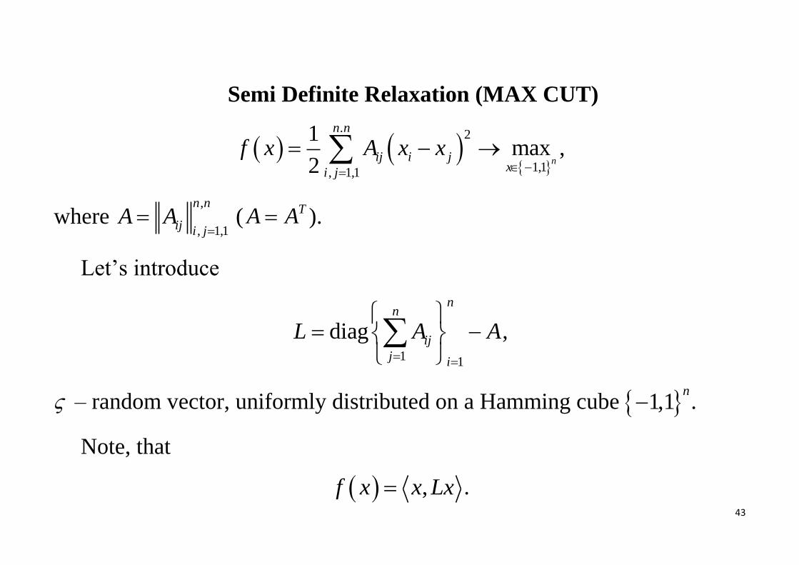
Semi Definite Relaxation (MAX CUT)
.2
1,1, 1,1
1max
2 n
n n
ij i jxi j
f x A x x
,
where ,
, 1,1
n n
ij i jA A
(
TA A ).
Let’s introduce
1 1
diag
nn
ij
j i
L A A
,
– random vector, uniformly distributed on a Hamming cube 1,1n
.
Note, that
,f x x Lx .
44
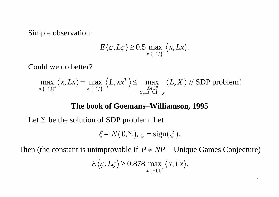
Simple observation:
1,1
, 0.5 max ,n
x
E L x Lx
.
Could we do better?
1,1 1,11, 1,...,
max , max , max ,n n n
ii
T
X Sx xX i n
x Lx L xx L X
// SDP problem!
The book of Goemans–Williamson, 1995
Let be the solution of SDP problem. Let
0,N , sign .
Then (the constant is unimprovable if P NP – Unique Games Conjecture)
1,1
, 0.878 max ,n
x
E L x Lx
.

45
“Optimal” methods aren’t always optimal indeed
We can reduce Google problem to
2
2 1
1min ,
2 nx Sf x Ax
We will use not optimal (in terms the number of oracle calls) conditional
gradient method (Frank–Wolfe, 1956). But we assume that the number of
nonzero elements at each row and each column smaller then s n .
We choose starting point at one of the simplex vertex 1x . Induction step
1
, minn
k
y Sf x y
.
Let’s denote the solution of this problem by
46
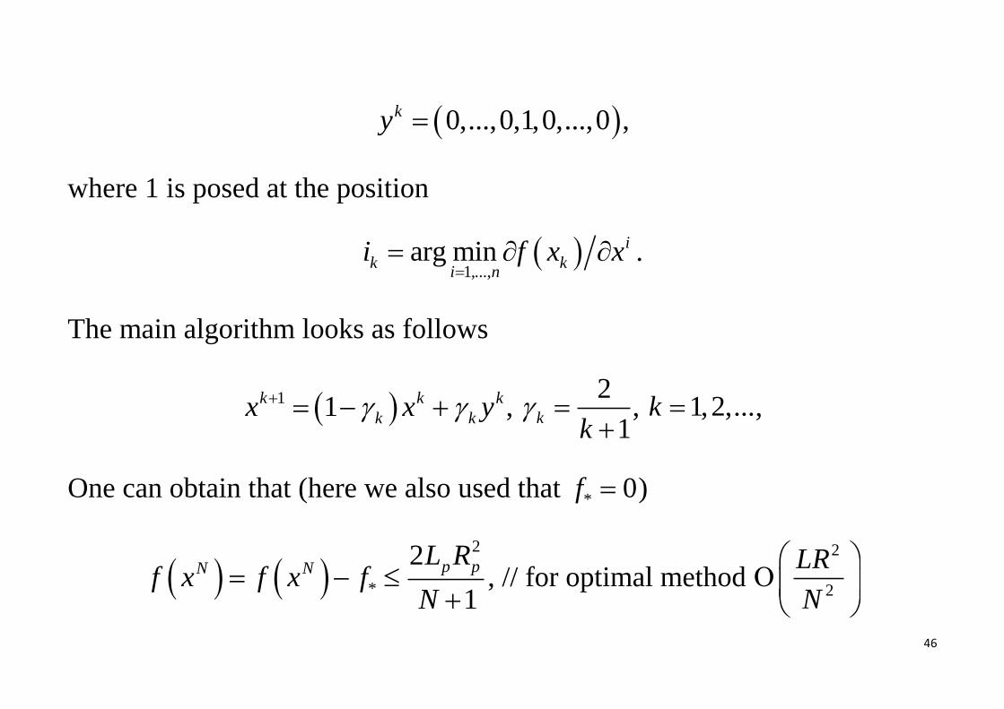
0,...,0,1,0,...,0ky ,
where 1 is posed at the position
1,...,
arg min i
k ki n
i f x x
.
The main algorithm looks as follows
1 1k k k
k kx x y , 2
1k
k
, 1,2,...k ,
One can obtain that (here we also used that * 0f )
2
*
2
1
p pN NL R
f x f x fN
, // for optimal method 2
2
LR
N
47
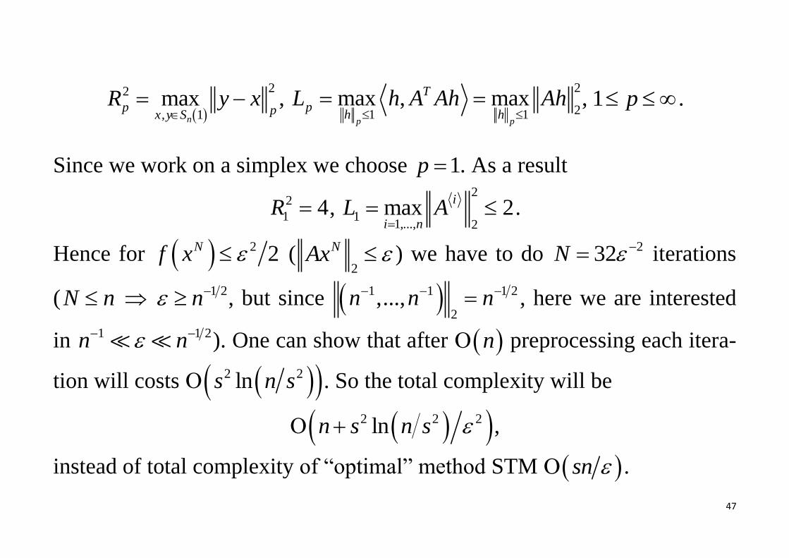
22
, 1max
n
p px y SR y x
,
2
21 1max , max
p p
T
ph h
L h A Ah Ah
, 1 p .
Since we work on a simplex we choose 1p . As a result
2
1 4R , 2
11,..., 2
max 2i
i nL A
.
Hence for 2 2Nf x (2
NAx ) we have to do 232N iterations
(N n 1 2n , but since 1 1 1 2
2,...,n n n , here we are interested
in 1 1 2n n ). One can show that after n preprocessing each itera-
tion will costs 2 2lns n s . So the total complexity will be
2 2 2lnn s n s ,
instead of total complexity of “optimal” method STM sn .

48
Спасибо за внимание.