complex terrain module€¦ · the adms complex terrain module models dispersion over hills and...

August 2017 P14/01S/17

of 38

COMPLEX TERRAIN MODULE

CERC

In this document ‘ADMS’ refers to ADMS 5.2, ADMS-Roads 4.1, ADMS-Urban 4.1 and

ADMS-Airport 4.1. Where information refers to a subset of the listed models, the model name is

given in full.

CONTENTS

1. Introduction

2. FLOWSTAR

3. Flow around hills in Stable Conditions

4. Regions of Reverse Flow

5. Concentration Calculations

6. Example Model Output

7. References

Appendix A: Description of FLOWSTAR algorithms

Appendix B: Description of Stable Flow algorithms

Appendix C: Description of Reverse Flow algorithms

P14/01S/17 of 38

1. Introduction

The ADMS complex terrain module models dispersion over hills and regions with varying

surface roughness. The flow and turbulence fields over the complex terrain are calculated, and

used to adjust the plume height and plume spread parameters calculated by the flat terrain model.

The model takes account of all common cases where the ‘mean’ wind dominates the flow. It

does not take account of thermal winds.

In most situations the flow and turbulence fields are calculated using the FLOWSTAR model,

which is described in Section 2. In very stable conditions, the flow field may divide, with air at

low levels flowing around rather than over the hills. The treatment of these conditions in ADMS

is described in Section 3. Section 4 outlines the treatment of plumes emitted into regions of

reverse flow. Section 5 describes the adjustment of the plume parameters, once the flow field has

been calculated.

2. FLOWSTAR

2.1 Introduction

FLOWSTAR calculates the flow field and turbulence parameters over complex terrain using

linearised analytical solutions of the momentum and continuity equations. An overview of the

calculation procedure is given below. A full description of the underlying theory is given in

Appendix A.

2.2 Input data

As input, FLOWSTAR requires data on the terrain height and surface roughness. FLOWSTAR

uses the same meteorological data as the main ADMS model. Boundary layer parameters are

calculated using the ADMS boundary layer structure module.

In line with the assumptions on which the model is based, terrain should have no more than

moderate slopes (up to 1:3) although the model is useful even when this criterion is not met (say

up to 1:2). It is not recommended that the model be used unless hill slopes are greater than about

1:10.

The data input by the user in the terrain file can be at any grid size, and the grid does not have to

be regular. However, the maximum number of data points in the terrain file is 66,000.

The input terrain data file takes the following form:

1, , ,

2, , ,

. . . .

. . . .

, , , . . . .

. . . .

, , ,

P14/01S/17 of 38

where is the index (number) of the point with position and is its elevation. For

example, in a domain 20km x 20km with 4096 regularly spaced points of data the terrain would

be specified at points approximately 320m apart.

If the surface roughness varies across the domain, surface roughness data may be entered in the

same way. If the roughness is assumed constant across the domain, one value is supplied to the

model, rather than gridded data.

2.3 Calculation methodology

For each wind direction a wind-aligned rectangle is described around the terrain points. Points in

the corners of the wind-aligned rectangle are assigned the mean terrain height over the boundary

of the user input domain. An internal calculation grid is set up over the rectangle. This grid is

regularly spaced and may have up to 256x256 points in the horizontal, the resolution being

selected by the user in the model interface. The number of points on the calculation grid affects

the model speed, memory requirement and model solution. A 64x64 grid is recommended for

most practical applications with slopes up to 1:3 if the domain is not large (not more than 10 km

x 10 km). The grid has 17 vertical levels ranging from 1.3 times the minimum surface roughness

to 5 km.

Fourier transforms of the terrain and roughness data are calculated and the flow solution is

calculated by inverting the Fourier transformed solution. In these calculations, the atmosphere is

split into three layers:

i) the inner layer, close to the ground, where shear stress perturbations must be taken into

account but stratification is unimportant

ii) the middle layer, far enough from the ground that shear stresses are not important but the

effects of stress are; again stratification is unimportant

iii) the outer layer, where shear is unimportant, but stratification must be taken into account.

Two stratification cases are considered in ADMS, corresponding to stable conditions with a

uniform density gradient and neutral or unstable conditions where there is an inversion and

discontinuity in density at a certain height , constant density below and a uniform density

gradient above .

2.4 Output

The outputs of the model are:

(i) local mean wind velocity components

(ii) local root mean square velocity scales , ,

(iii) vertical and transverse length scales and

(iv) Lagrangian time scale

(v) energy dissipation rate

These variables are used to adjust the plume parameters calculated by the flat terrain model (see

Section 5).

P14/01S/17 of 38

3. Flow around hills in Stable Conditions

3.1 Introduction

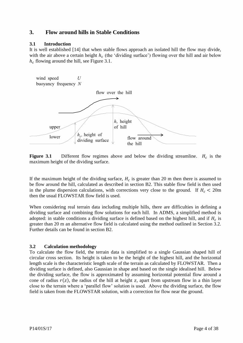
It is well established [14] that when stable flows approach an isolated hill the flow may divide,

with the air above a certain height (the ‘dividing surface’) flowing over the hill and air below

flowing around the hill, see Figure 3.1.

Figure 3.1 Different flow regimes above and below the dividing streamline. is the

maximum height of the dividing surface.

If the maximum height of the dividing surface, is greater than 20 m then there is assumed to

be flow around the hill, calculated as described in section B2. This stable flow field is then used

in the plume dispersion calculations, with corrections very close to the ground. If 20m

then the usual FLOWSTAR flow field is used.

When considering real terrain data including multiple hills, there are difficulties in defining a

dividing surface and combining flow solutions for each hill. In ADMS, a simplified method is

adopted: in stable conditions a dividing surface is defined based on the highest hill, and if is

greater than 20 m an alternative flow field is calculated using the method outlined in Section 3.2.

Further details can be found in section B2.


To calculate the flow field, the terrain data is simplified to a single Gaussian shaped hill of

circular cross section. Its height is taken to be the height of the highest hill, and the horizontal

length scale is the characteristic length scale of the terrain as calculated by FLOWSTAR. Then a

dividing surface is defined, also Gaussian in shape and based on the single idealised hill. Below

the dividing surface, the flow is approximated by assuming horizontal potential flow around a

cone of radius , the radius of the hill at height , apart from upstream flow in a thin layer

close to the terrain where a ‘parallel flow’ solution is used. Above the dividing surface, the flow

field is taken from the FLOWSTAR solution, with a correction for flow near the ground.

P14/01S/17 of 38

4. Regions of Reverse Flow

4.1 Introduction

A source located within a region of reverse flow (i.e. a region where the wind velocity

component in the free stream wind direction is negative) may lead to high concentrations

upstream of the source.

In ADMS it is assumed that a plume released into a reverse flow region is well-mixed within that

region. The release is represented downwind of that region by dispersion from a virtual source.

This is closely analogous to the treatment of plumes entrained into the near wake (‘recirculating

region’) of a building in the ADMS buildings module. However, unlike the buildings module,

the case of a plume being partially entrained into the near wake is not treated. Currently only

plumes released into a reverse flow region are treated – the plume is not permitted to enter a

reverse flow region after release.


An ‘effective source height’ is defined, which includes the initial effects of buoyancy and

momentum of the release. If the downwind velocity component at the effective source is

negative (i.e. the effective source is in a reverse flow region), then the full extent of the reverse

flow region is found. An ‘effective recirculation zone’ is then defined (Figure 4.1), throughout

which the contaminant is assumed to be well-mixed. The concentration is assumed to be uniform

within this ‘effective recirculation zone’. The effective recirculation zone may be the same as the

recirculation zone or may be contained within it, for instance if the zone is very wide.

At the downstream edge of this zone, the plume dispersion parameters ( and are estimated

based on the cross-stream dimensions of the effective recirculation zone. These parameters are

used in the subsequent calculations of plume concentration to represent dispersion from a ‘virtual

source’, or a number of ‘virtual sources’ if the original source has a large crosswind extent. The

plume from each virtual source is assumed to be passive.

For an effective source outside the reverse flow region the plume dispersion calculations are

influenced by a reverse flow region only if the plume centre line enters the region. No partial

entrainment of the plume is assumed. If reverse flow is encountered by the plume centreline,

then the plume height is increased until it is within a region of forward flow.

Full details of the calculation procedure are given in Appendix C.

P14/01S/17 of 38

Wind

Figure 4.1 The recirculating region and effective recirculating region

‘Effective

recirculation

region’

HILL

Plume from ‘virtual

source’

Source

Recirculation

region

P14/01S/17 of 38

5. Concentration calculations

5.1 Introduction

To calculate concentrations over complex terrain, the calculated flow and turbulence fields are

used to make adjustments to the plume height and plume spread parameters. Concentration

calculations then proceed using the same methods as the flat terrain module.

5.2 Plume centreline height

In the ADMS flat terrain module, the change in plume height between downstream calculation

points and , say, includes contributions from plume rise and gravitational settling. In the

complex terrain module, an extra contribution from the terrain effects is included. This is

calculated by following a streamline downwind from the initial plume position. The wind

velocity field at the initial plume centreline position ( , , ) is calculated by linear

interpolation between points on the FLOWSTAR calculation grid. The model then steps

downstream along the streamline to to calculate the adjusted crosswind plume position and

plume centreline height . With variable roughness, the velocity profile near the ground is

adjusted to be zero at the local roughness height.

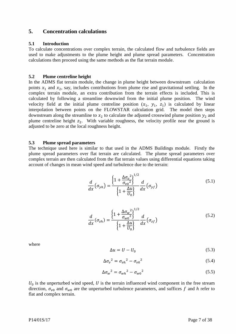
5.3 Plume spread parameters

The technique used here is similar to that used in the ADMS Buildings module. Firstly the

plume spread parameters over flat terrain are calculated. The plume spread parameters over

complex terrain are then calculated from the flat terrain values using differential equations taking

account of changes in mean wind speed and turbulence due to the terrain:

(5.1)

(5.2)

where

(5.3)

(5.4)

(5.5)

is the unperturbed wind speed, is the terrain influenced wind component in the free stream

direction, and are the unperturbed turbulence parameters, and suffices and refer to

flat and complex terrain.

P14/01S/17 of 38

6. Example Model Output

Example flow and concentration fields for a simple Gaussian hill are shown below. The input

terrain is illustrated in Figure 6.1. The terrain has been modelled under neutral meteorological

conditions, with a westerly wind of speed 5 m/s. The resulting flow field at 10 m above the

terrain is illustrated in Figure 6.2.

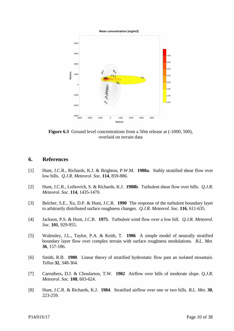
A source of height 50 m with a passive release of 1 g/s was included at (-1000, 500). Figure 6.3

shows the resulting ground level concentrations.

Figure 6.1 Input terrain data

P14/01S/17 of 38

Figure 6.2 Wind field at 10 m above terrain, neutral conditions

-3000.00 -2000.00 -1000.00 0.00 1000.00 2000.00 3000.00 4000.00

Metres

Component of mean wind from West (U), m/s, at height 10m

-3000.00

-2000.00

-1000.00

0.00

1000.00

2000.00

3000.00

4000.00

Me

tre

s

-3000.00 -2000.00 -1000.00 0.00 1000.00 2000.00 3000.00 4000.00

Metres

Component of mean wind from South (V), m/s, at height 10m

-3000.00

-2000.00

-1000.00

0.00

1000.00

2000.00

3000.00

4000.00

Me

tre

s

-3000.00 -2000.00 -1000.00 0.00 1000.00 2000.00 3000.00 4000.00

Metres

Mean vertical velocity (W), m/s, at height 10m

-3000.00

-2000.00

-1000.00

0.00

1000.00

2000.00

3000.00

4000.00

Metr

es

P14/01S/17 of 38

Figure 6.3 Ground level concentrations from a 50m release at (-1000, 500),

overlaid on terrain data

6. References

[1] Hunt, J.C.R., Richards, K.J. & Brighton, P.W.M. 1988a. Stably stratified shear flow over

low hills. Q.J.R. Meteorol. Soc. 114, 859-886.

[2] Hunt, J.C.R., Leibovich, S. & Richards, K.J. 1988b. Turbulent shear flow over hills. Q.J.R.

Meteorol. Soc. 114, 1435-1470.

[3] Belcher, S.E., Xu, D.P. & Hunt, J.C.R. 1990 The response of the turbulent boundary layer

to arbitrarily distributed surface roughness changes. Q.J.R. Meteorol. Soc. 116, 611-635.

[4] Jackson, P.S. & Hunt, J.C.R. 1975. Turbulent wind flow over a low hill. Q.J.R. Meteorol.

Soc. 101, 929-955.

[5] Walmsley, J.L., Taylor, P.A. & Keith, T. 1986 A simple model of neutrally stratified

boundary layer flow over complex terrain with surface roughness modulations. B.L. Met.

36, 157-186.

[6] Smith, R.B. 1980. Linear theory of stratified hydrostatic flow past an isolated mountain.

Tellus 32, 348-364.

[7] Carruthers, D.J. & Choularton, T.W. 1982 Airflow over hills of moderate slope. Q.J.R.

Meteorol. Soc. 108, 603-624.

[8] Hunt, J.C.R. & Richards, K.J. 1984. Stratified airflow over one or two hills. B.L. Met. 30,

223-259.

-3000 -2000 -1000 0 1000 2000 3000 4000

Metres

Mean concentration (mg/m3)

-3000

-2000

-1000

0

1000

2000

3000

4000

Metr

es

0.50

1.00

2.00

3.00

4.00

5.00

6.00

7.00

P14/01S/17 of 38

[9] Wieringa, J. 1976 An objective exposure correction method for average wind speeds

measured at a sheltered location. Q.J.R. Meteorol. Soc. 10, 241-253.

[10] Abramowitz, M. & Stegun, I.A. 1972 Handbook of Mathematical Functions. Dover

Publications Inc., New York.

[11] Finnigan, J.J. 1988 Airflow over complex terrain. In Flow and Transport in the Neutral

Environment: Advances and Applications (eds. W.K. Steffen and O.T. Denmead).

Springer-Verlag, Heidelberg.

[12] Carruthers, D.J. & Hunt, J.C.R. 1990 Fluid mechanics of airflow over hills: Turbulence,

fluxes and waves in the boundary layer. AMS Monograph.

[13] Hunt, J.C.C., Holroyd, R.J. & Carruthers D.J. 1988 Preparatory studies for a complex

dispersion model. Report to NRPB, AWE, HMIP, HSE. CERC Ltd.

[14] Weng, W.S., Richards, K.J. & Carruthers, D.J. 1988 Some numerical studies of turbulent

airflow over hills. Proc. 2nd European Turbulence Conf. Aug. 1988 (eds. Fernholz &

Fiedler).

[15] Hunt, J.C.R. 1985 Turbulent diffusion from sources in complex flows. Ann. Rev. Fluid

Mech. 17, 447-485

[16] Lavery, T.F., Bass, A., Strimaitism, D.G., Venkatram, A., Green, B.R., Drivas, P.J., &

Egan, B.A. 1981 EPA complex model development. 1st Milestone Report.

[17] Newley, T.J. 1986 Turbulent airflow over hills. Ph.D thesis, Cambridge University.

P14/01S/17 of 38

APPENDIX A: Description of FLOWSTAR algorithms

Contents

A1. Summary

A2. Overview of the model and the computational procedure

A2.1 Background and previous work

A2.2 Description of the analytical model and its physical implications

A2.3 Main elements in the computational model, software and use procedure

A3. Procedure and algorithms for computing mean flow over hills

A3.1 Terrain height and lateral scale

A3.2 Roughness length z0 over the terrain

A3.3 Specifying the upwind meteorology

A3.4 Calculating the length scales and dimensional groups

A3.5 Calculating the velocity and streamline deflections

A3.6 Calculating the velocity due to roughness changes

A3.7 Algorithms for the shear stress and surface shear stress

A3.8 Algorithms for turbulence

P14/01S/17 of 38

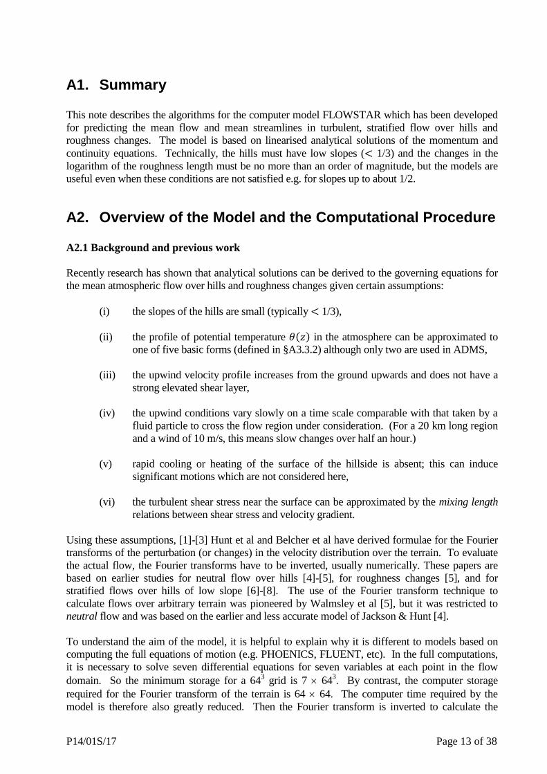
A1. Summary

This note describes the algorithms for the computer model FLOWSTAR which has been developed

for predicting the mean flow and mean streamlines in turbulent, stratified flow over hills and

roughness changes. The model is based on linearised analytical solutions of the momentum and

continuity equations. Technically, the hills must have low slopes ( 1/3) and the changes in the

logarithm of the roughness length must be no more than an order of magnitude, but the models are

useful even when these conditions are not satisfied e.g. for slopes up to about 1/2.

A2. Overview of the Model and the Computational Procedure

A2.1 Background and previous work

Recently research has shown that analytical solutions can be derived to the governing equations for

the mean atmospheric flow over hills and roughness changes given certain assumptions:

(i) the slopes of the hills are small (typically 1/3),

(ii) the profile of potential temperature in the atmosphere can be approximated to

one of five basic forms (defined in §A3.3.2) although only two are used in ADMS,

(iii) the upwind velocity profile increases from the ground upwards and does not have a

strong elevated shear layer,

(iv) the upwind conditions vary slowly on a time scale comparable with that taken by a

fluid particle to cross the flow region under consideration. (For a 20 km long region

and a wind of 10 m/s, this means slow changes over half an hour.)

(v) rapid cooling or heating of the surface of the hillside is absent; this can induce

significant motions which are not considered here,

(vi) the turbulent shear stress near the surface can be approximated by the mixing length

relations between shear stress and velocity gradient.

Using these assumptions, [1]-[3] Hunt et al and Belcher et al have derived formulae for the Fourier

transforms of the perturbation (or changes) in the velocity distribution over the terrain. To evaluate

the actual flow, the Fourier transforms have to be inverted, usually numerically. These papers are

based on earlier studies for neutral flow over hills [4]-[5], for roughness changes [5], and for

stratified flows over hills of low slope [6]-[8]. The use of the Fourier transform technique to

calculate flows over arbitrary terrain was pioneered by Walmsley et al [5], but it was restricted to

neutral flow and was based on the earlier and less accurate model of Jackson & Hunt [4].

To understand the aim of the model, it is helpful to explain why it is different to models based on

computing the full equations of motion (e.g. PHOENICS, FLUENT, etc). In the full computations,

it is necessary to solve seven differential equations for seven variables at each point in the flow

domain. So the minimum storage for a 643 grid is 7 64

3. By contrast, the computer storage

required for the Fourier transform of the terrain is 64 64. The computer time required by the

model is therefore also greatly reduced. Then the Fourier transform is inverted to calculate the

P14/01S/17 of 38

actual flow variables at any point in the calculation domain, without the need for iteration and there

is no doubt about the convergence of the solution once the algorithm and its assumptions have been

agreed. This is why the Fourier transform method is quite appropriate for use on desktop

computers.

We now introduce the physical ideas behind the three-layer model for the flow.

A2.2 Description of the analytical model and its physical implications

In the solution for the airflow over hills used to produce the algorithms, the lower atmosphere is

divided into three layers: the inner layer, the middle layer and the outer layer.

The inner layer contains the layer near the ground in which the perturbation shear stresses are

important. Using a closure based on local equilibrium of turbulence for the shear stress, Bessel

equations are obtained for the perturbation velocities.

The middle layer is sufficiently far above the ground that shear stresses are unimportant. However,

the effects of shear are important. In both the inner layer and the middle layer the effect of local

stratification is not significant, as air flows over the hill, although stratification may affect the

upwind profile.

The outer layer contains the outer part of the turbulent boundary layer and may also include part of

the free, non-turbulent atmosphere (e.g. in case , defined in §A3.3.2, the air above the inversion is

generally non-turbulent and does not form part of the boundary layer). In the outer layer

stratification now has an important effect but the shear and perturbation stress are unimportant. In

this layer we solve the equations for inviscid stratified flow. For example, the equation for , in 3-

D, is

where

Note that to a first order approximation it is the pressure field developed in the outer layer at the

boundary with the middle layer which drives the flow in the two lower layers. This pressure field is

strongly affected by stratification and so by this means flow in the lower layer is affected by

stratification in the outer layer.

In the neutral case, there is no stratification and the solution in the outer layer is potential flow; the

difference is confined close to the hill surface. Before describing the effects of discontinuities in

stratification we consider the stable case where there is uniform stratification (i.e. the buoyancy

frequency is constant with height). The equation shows that waves with frequency can propagate whilst waves with frequency are evanescent and thus decay away from the

surface. An upper boundary conditions has to be used for low frequency waves , so that

energy propagates upwards. This gives a downward phase velocity and the familiar asymmetrical

flow pattern with the strongest velocities downwind of the summit of the hill. The amount of flow

moving in horizontal planes around the hill increases with stratification.

P14/01S/17 of 38

In the second kind of stratification considered here, suitable for unstable conditions, there is an

inversion at height . Above the air is still stably stratified. Then waves with frequency

can propagate within and along the inversion layer but not in the upper layer above or

the middle layer below . It is found that energy may be trapped giving large-amplitude

perturbations which, in the atmosphere, appear downwind of the hill. In the linearised mode we

have to make an assumption about the amplitude of these resonant waves. We take a plausible

value, but recognise that this question has not been properly considered so far.

A2.3 Main elements in the computational model, software and user procedures

There are three main elements in the program and software to implement the model.

(i) Input

Receiving and storing the data about the terrain, roughness and meteorology (or upwind

flow). The data must be specified within a rectangular grid, but can be specified on grid

lines with irregular spacing.

(ii) Pre-processing

The input data is then processed to enable the flow computations to proceed. Chiefly, this

stage involves taking Fourier transforms of the terrain height and of the logarithm of the

roughness length over the flow region. It also involves defining the depths and of the

middle layer and inner region over the terrain.

(iii) Calculation

Computation of the distribution of the mean flow, turbulence and mean streamlines on the

internal calculation grid.

P14/01S/17 of 38

A3.Procedures and Algorithms for Computing Mean Flow over Hills

A3.1 Terrain height and lateral scale

(i) Terrain is specified within a domain which is a rectangle of side length

(typically 10 km).

(ii) The height of the terrain or is specified on an irregularly-spaced mesh on a

mesh scale of (i.e. is specified at points ). In general the input terrain

may be an irregular mesh, but the calculation is carried out on a regular grid, with 16 16,

32 32, 64 64, 128 128 or 256 256 points.

Figure A.1

A3.2 Roughness length over the terrain

The model can treat changes in surface roughness. Only the first-order solution is included in the

current algorithm. Belcher et al [3] showed that when second-order effects are included the

roughness changes lead to significant horizontal divergence which is absent from the first-order

solution. Advice on the choice of for different fetches of actual terrain (country, sea, suburbs,

etc) is given by, for example, Wieringa [9]. In the algorithms which follow is the surface

roughness, which may vary with position, is the value upstream and is the mean value over

the calculation domain.

A3.3 Specifying the upwind meteorology

A3.3.1 Input profile of wind

The stability-dependent input wind profiles are defined in the specification for the boundary layer

structure module (P09/01 ‘Boundary layer structure specification’) and are the same as for flat

terrain.

P14/01S/17 of 38

A3.3.2 Types of stratification

The type of stratification is defined in the outer layer. The middle and inner layers are effectively

neutral in all conditions considered in this model. Note however, that the height of the middle and

upper layer may be wave-number dependent. The buoyancy frequency is defined by

(A3.1)

where is the potential temperature.

Five stratification cases can be considered by FLOWSTAR, namely:

(i) - neutral

(ii) - uniform density, gradient and uniform wind speed ( constant with height);

(iii) - zero density gradient below inversion , density discontinuity and uniform density gradient above inversion .

(iv) - strong inversion layer capping a uniformly stratified boundary layer, stable

uniform density gradient below inversion;

(v) - lower layer gradually decreasing stratification up to an upper layer of constant

stratification.

Only profiles (ii) and (iii) are currently used in ADMS.

A3.4 Calculating length scales and dimensionless groups

A3.4.1 Definition of the characteristic half length of the terrain

(A3.2)

where

(A3.3)

If the calculation mesh size selected is greater than 32 32, only the smallest 32 wavenumbers are

included in this calculation. This ensures that represents the dominant features of the terrain.

The Fourier transform of the terrain is given by

(A3.4)

P14/01S/17 of 38

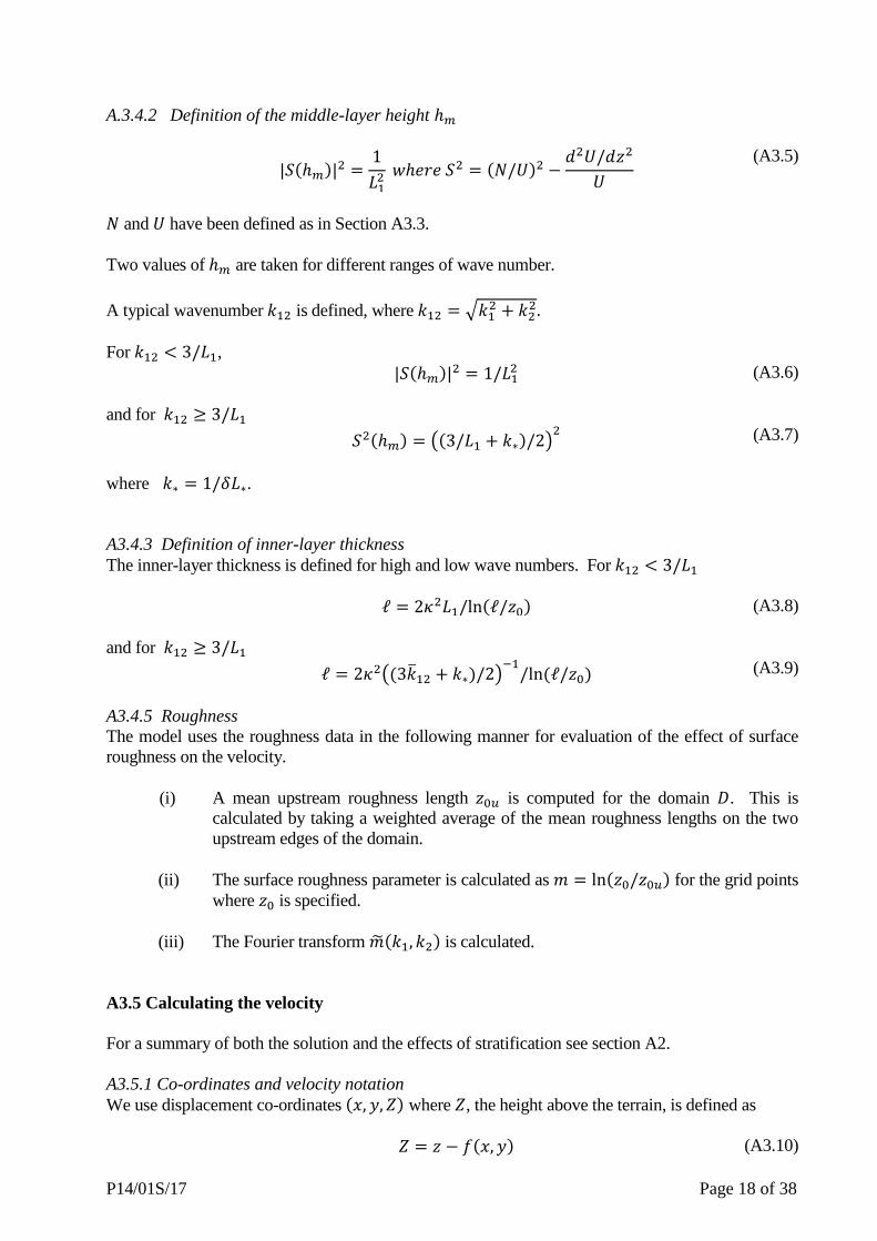
A.3.4.2 Definition of the middle-layer height

(A3.5)

and have been defined as in Section A3.3.

Two values of are taken for different ranges of wave number.

A typical wavenumber is defined, where

For ,

(A3.6)

and for

(A3.7)

where .

A3.4.3 Definition of inner-layer thickness

The inner-layer thickness is defined for high and low wave numbers. For

(A3.8)

and for

(A3.9)

A3.4.5 Roughness

The model uses the roughness data in the following manner for evaluation of the effect of surface

roughness on the velocity.

(i) A mean upstream roughness length is computed for the domain . This is

calculated by taking a weighted average of the mean roughness lengths on the two

upstream edges of the domain.

(ii) The surface roughness parameter is calculated as for the grid points

where is specified.

(iii) The Fourier transform is calculated.

A3.5 Calculating the velocity

For a summary of both the solution and the effects of stratification see section A2.

A3.5.1 Co-ordinates and velocity notation

We use displacement co-ordinates where , the height above the terrain, is defined as

(A3.10)

P14/01S/17 of 38

Let be the upwind velocity at the height above the surface.

Figure A.2

The components of the velocities are

(A3.11a)

(A3.11b)

(A3.11c)

where , and are perturbations caused by the changes in elevation, and and are

perturbations caused by roughness changes.

We denote the Fourier transform by , thus

(A3.12)

The general form of solutions for (ud, vd, wd) is:

(A3.13)

(A3.14)

(A3.15)

where . For , the expression for is written in real space as

P14/01S/17 of 38

(A3.16)

where represents the inverse Fourier transform and where etc. are factors defined in Section

A3.5.3 below.

A3.5.2 General middle and inner-layer structure

Same form for most conditions when stratified (provided 1, and 1/2).

Note:

(A3.17)

(A3.18)

(A3.19)

where is the approximate second-order correction term. The dimensionless parameters , ,

, and are defined as follows.

For ,

(A3.20)

For ,

0.4

and the modified Bessel function can be expressed as

(A3.21)

P14/01S/17 of 38

where or or

Note that the Kelvin functions, and , are computed using polynomial approximations [10].

To make sure the solutions are continuous at , we use blending functions to match the

solutions in the inner region and middle layer. For

(A3.22)

and for

(A3.23)

where and are the functions in the inner region and middle layer respectively for the -

direction and and are the functions for the -direction.

A3.5.3 Upper-layer functions for different stratification cases

(i) Neutral ( )

(A3.24)

(A3.25)

(ii) Stable ( Uniform in upper layer)

(A3.26)

(note is wavenumber dependent)

(A3.27)

(A3.28)

If

(A3.29)

and

P14/01S/17 of 38

(A3.30)

(iii) Convective ( Inversion at with stable layer above and well-mixed layer below)

For ,

(A3.31)

where is a step function, i.e.

above inversion,

below inversion.

(A3.32)

The Froude number of the inversion layer, , is given by

(A3.33)

In order to define the user specifies the potential temperature step , and the

potential temperature .

For ,

(A3.34a)

(A3.34b)

and for ,

(A3.35a)

(A3.35b)

where

(A3.36)

P14/01S/17 of 38

where is a damping term introduced to avoid singularities due to trapped waves.

P14/01S/17 of 38

A3.6 Algorithm for roughness change

This is a first-order calculation, which gives the Fourier transform of the perturbation to due to the

roughness changes, and . ( 0 to this order of accuracy). The Fourier transform of the

roughness perturbation is largely determined by the roughness parameter . The solutions are

(A3.37a)

(A3.37b)

where

(A3.38a)

where is the upstream roughness (taken to be the mean value along the two upstream edges

of the domain), and is a ‘boundary condition’ roughness, set as follows:

• If is the minimum roughness over the domain, then is the maximum roughness

over the domain

• If is the maximum roughness over the domain, then is the minimum roughness

over the domain

• If is neither the maximum nor the minimum roughness, then is the maximum

roughness over the domain

and

(A3.38b)

(A3.38c)

(A3.38d)

so that has to be evaluated for each wavenumber.

This means that the perturbation may be overestimated where the local roughness is less than the

maximum roughness, but this can be counteracted (in a simple way) by constraining the vertical

profile of to lie between the two profiles

(A3.38e)

and

P14/01S/17 of 38

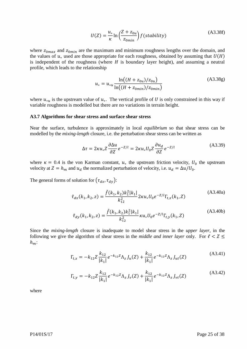
(A3.38f)

where and are the maximum and minimum roughness lengths over the domain, and

the values of used are those appropriate for each roughness, obtained by assuming that is independent of the roughness (where is boundary layer height), and assuming a neutral

profile, which leads to the relationship

(A3.38g)

where is the upstream value of . The vertical profile of is only constrained in this way if

variable roughness is modelled but there are no variations in terrain height.

A3.7 Algorithms for shear stress and surface shear stress

Near the surface, turbulence is approximately in local equilibrium so that shear stress can be

modelled by the mixing-length closure, i.e. the perturbation shear stress can be written as

(A3.39)

where 0.4 is the von Karman constant, the upstream friction velocity, the upstream

velocity at and the normalized perturbation of velocity, i.e. .

The general forms of solution for :

(A3.40a)

(A3.40b)

Since the mixing-length closure is inadequate to model shear stress in the upper layer, in the

following we give the algorithm of shear stress in the middle and inner layer only. For :

(A3.41)

(A3.42)

where

P14/01S/17 of 38

(A3.43)

In the inner region

(A3.44a)

(A3.44b)

where

(A3.45)

The surface shear stress is given by

(A3.46a)

(A3.46b)

(for the definitions of some parameters see section A3.5.2.)

The algorithm for the shear stress perturbation due to roughness changes is given by

P14/01S/17 of 38

(A3.47)

A3.8 Algorithms for turbulence

A3.8.1 Turbulent velocities

For the calculation of the turbulence components, estimates using the calculated shear stress are

made in the inner region, while rapid distortion theory is used in the upper part of the middle and

outer regions since the structure in these regions is determined by the distortion of the upwind

turbulence structure. Between these two regions there is a layer where there are a number of effects

determining the structure of the turbulence including advection, distortion, curvature and local non-

linear effects [11]. It is not possible to calculate these effects within an approach suitable for

diffusion, so since we know from observations that the turbulent velocities do not obtain locally

large values in this region, we use a blending function to match the solution in the inner and outer

regions across this layer [12].

Upwind the profiles are as defined in the Boundary Layer Structure Specification.

For the blending functions, we use in the inner region

(A3.48a)

(A3.48b)

and in the outer region

(A3.49a)

(A3.49b)

The expressions for the turbulence components over the hill are then

(A3.50)

(A3.51)

(A3.52)

where for upwind isotropic turbulence 2/5 and we have taken a value for the factor 2.

P14/01S/17 of 38

The

term in equation A3.52 has been introduced to account for the increase in vertical turbulence

in the lee of the hill. The constant factor takes the value 5, and

is the Heaviside step

function of

.

The suffixes and denote the upstream contribution from mechanically driven turbulence

( term) and convectively driven turbulence ( term).

The blending functions are such that the solutions are continuous at . The factors , ,

have been introduced to allow for the decrease in the upwind turbulence energy with height ([3],

1988). They are defined as follows:

In convective or neutral conditions,

(A3.53a)

In stable conditions,

(A3.53b)

In addition, a minimum value of 0.1 m/s is imposed on , , and .

In the above formulation for turbulence it is assumed that mechanically driven turbulence dominates

convectively produced turbulence. However in moderate or strongly convective conditions this

condition is no longer held. In those situations which occur in stratification case 2 when Monin-

Obukhov length 0, we include a contribution to the turbulent velocities due to convection;

this contribution is not affected by the flow over the hills.

A3.8.2 Turbulent length scales

Following Weng et al [14], we assume a vertical length scale including the effects of local shear, i.e.

(A3.54a)

where the constants are 0.6 and 1.0. For the transverse length scale an appropriate

expression is

P14/01S/17 of 38

(A3.54b)

where

is a local length scale which could be taken equal to

. However, for simplicity and in

view of the fact that does not change significantly we take

.

, , where is the boundary layer depth.

P14/01S/17 of 38

APPENDIX B: Description of Stable Flow Algorithms

Contents

B1. Introduction

B2. Calculation of stable flow field

B2.1 Definition of idealised hill

B2.2 Definition of dividing surface

B2.3 Calculation of flow field

B2.4 Calculation of turbulence parameters

B1 Introduction

It is well established that when stable flows approach an isolated hill, the flow may

divide with the air above a certain height, , flowing over the hill and air below

flowing around the hill, see Figure B.1. is the height of what is called the dividing

streamline in 2-dimensions, or, in 3-dimensions, the dividing surface.

Figure B.1 Different flow regimes above and below the dividing surface

P14/01S/17 of 38

A critical value of 20 m is applied to the maximum dividing surface height, . If

20m then the method described in this section is applied based on a Gaussian

shaped hill. (Note that variable roughness has no effect on the flow below the

dividing streamline in this regime.) This stable flow field is used for the dispersion

calculations over the whole domain. If 20m then the usual FLOWSTAR flow

field is used

In stable conditions, an adjusted buoyancy frequency, , is used in the

FLOWSTAR solution, calculated by

where is the standard buoyancy frequency and is the height of the highest hill.

This adjustment improves the FLOWSTAR solution for stable flows.

B2 Calculation of stable flow field

Suppose the input terrain data have height , denotes height above sea level,

the height above the terrain, the velocity field relative to the terrain at point

is , and the velocity field relative to sea level is .

B2.1 Definition of idealised hill

The idealised hill is assumed to be Gaussian in shape with circular horizontal cross-

section. The height of the hill is the maximum height of the input terrain, , and

is centred on the point where the input terrain maximum occurs, see Figure B.2. The

height of the idealised hill, , where and are Cartesian co-ordinates with

origin at the centre of the hill, is given by:

where is a characteristic length scale for the input terrain: , where

, the characteristic lengthscale in the alongwind direction, is given by A3.3, and ,

the characteristic lengthscale in the crosswind direction, is calculated similarly using

instead of .

P14/01S/17 of 38

Figure B.2 Definition of idealised hill and dividing surface

B2.2 Definition of dividing surface

The dividing surface, illustrated in Figure B.2, is also assumed to be Gaussian in

shape and its height is given by:

Here is a constant set to 10, and is the maximum height of the dividing surface

which is defined by an energy balance equation which locates the lowest height at

which the kinetic energy of an air parcel in the flow approaching the hill is equal to

the potential energy attained by elevating an equivalent fluid parcel from this height

to the top of the hill:

B2.3 Calculation of flow field

B2.3.1 Below the dividing surface

Below the dividing surface, the flow is two dimensional. The majority of the flow is

potential flow. In a small region close to the terrain however (less than 10 m from the

terrain surface) upstream flow is forced to flow parallel to the terrain. This means that

the plume will travel around the hill. Figure B.3 gives a schematic diagram of this

flow.

hmax

real terrain

idealised hill

dividing surface

P14/01S/17 of 38

Figure B.3 Stable flow close to the terrain

The mathematical formulation of the potential and parallel flows are given below.

Potential flow

We assume horizontal flow around a cone of radius , where is the radius of

the idealised hill, at height .

where

The vertical velocity is zero relative to the terrain, so

0

Parallel flow

Upstream flow close to the terrain is parallel to the terrain. The flow field here takes

the form

where

y=0

upstream flow

f(x,y) = C, a

constant

a constant

KEY:

parallel flow

potential flow

P14/01S/17 of 38

Again, the vertical velocity is zero relative to the terrain, so

0

B2.3.2 Above the dividing surface

Above the FLOWSTAR flow field is used, except in a thin layer close to the

ground where a scaling is applied between flow parallel to the ground and the

FLOWSTAR solution. The flow parallel to the ground is given by:

0

0

B2.4 Calculation of turbulence parameters

The turbulence parameters are scaled by a factor , which is the ratio of the terrain-

influenced and unperturbed horizontal wind speeds, i.e.

where

P14/01S/17 of 38

APPENDIX C: Description of Reverse Flow algorithms

Contents

C1. Introduction

C2. General method

C3. Recirculating region

C4. Calculation of concentration

C1 Introduction

A source located wholly or partly within a region of recirculating flow may lead to

high concentrations upstream of the source (relative to the free stream wind

direction).

In ADMS it is assumed that the plume is well-mixed within the recirculation zone and

is represented downwind of that region by dispersion from a virtual source or sources.

This is closely analogous to the treatment of plumes entrained into the near wake of a

building in the ADMS buildings module. However, unlike the buildings module, the

case of a plume being partially entrained into the recirculation zone is not treated.

C2 General method

An ‘effective source height’ is defined, which includes the initial effects of buoyancy

and momentum of the release. If the wind speed at the effective source is negative

(i.e. the effective source is in a reverse flow region), then the full extent of the reverse

flow region is found. An ‘effective recirculation zone’ is then defined (Figure C.1),

throughout which the contaminant is assumed to be well-mixed. The concentration is

assumed to be uniform within this ‘effective recirculation zone’. The effective

recirculation zone may be the same as the recirculation zone or may be contained

within it, for instance if the zone is very wide.

At the downstream edge of this zone, the plume dispersion parameters ( and ) are

estimated based on the cross-stream dimensions of the effective recirculation zone.

These parameters are used in the subsequent calculations of plume concentration to

represent dispersion from a ‘virtual source’ at the downstream edge of the zone, or, if

the original source has significant crosswind extent, from a series of ‘virtual sources’.

The plume from each virtual source is assumed to be passive.

For an effective source outside the reverse flow region the plume dispersion

calculations are influenced by a reverse flow region only if the plume centre line

enters the region. No partial entrainment of the plume is considered. If reverse flow is

encountered by the plume centreline, then the plume height is increased until it is

P14/01S/17 of 38

within a region of forward flow. The program will fail if this leads to a very large

discontinuity in the plume height (i.e. if , where is the

height of the plume centreline).

Wind

Figure C.1 The recirculating region and effective recirculating region

C3 Recirculating Region

The recirculating region is defined in the following manner:

(i) The top and bottom of the region and are set to the first heights

above and below the source height at which forward flow occurs.

(ii) The length of the recirculation region is calculated by finding the upwind

and downwind edges of the region that lie along a wind-aligned trajectory that

passes through the source, at a height 2.

(iii) The width of the region is calculated by finding the crosswind edges of

the region that lie along a trajectory perpendicular to the mean flow passing

through the source, at height 2.

By analogy with the building effects module, the recirculating flow region is assumed

well-mixed out to a maximum width where

where is the crosswind width of the source. If , the

effective well-mixed region, denoted , is the same as the recirculation region, .

Otherwise, is located within according to the lateral location of the source,

‘Effective

recirculation

region’

HILL

Plume from ‘virtual

source’

Source

Recirculation

region

P14/01S/17 of 38

such that is symmetric about the source position. If is within half the effective

width of a lateral edge of , then extends from that edge.

The volume occupied by the effective recirculation region is then given by

A residence time, , is calculated for the emission inside the effective recirculating

region:

where is the mean upstream wind speed at height .

C4 Calculation of concentration

There are three cases to consider for the concentration calculations depending on the

heights of the source and effective source relative to the reverse flow region.

(i) The source and effective source are above the reverse flow region

Concentrations are calculated using the usual method for flow over complex terrain.

(ii) The source is in the reverse flow region but the effective source is above it

The initial plume height is set equal to the effective source height. Concentrations are

calculated using the usual method for flow over complex terrain but with no further

plume rise due to buoyancy or momentum effects.

(iii) The source and effective source are within the reverse flow region

The concentration calculation is split into two parts: the concentration in the reverse

flow region and concentrations downstream of this region.

[1] The mean concentration inside the region is calculated by

assuming that all the emissions are entrained and that the region is

well-mixed. Then, applying a simple mass flux relationship

where is the source mass emission rate, is the residence time and

is the volume of the region.

[2] Concentrations downstream of the recirculating region are

determined by modelling a ‘virtual’ source at where

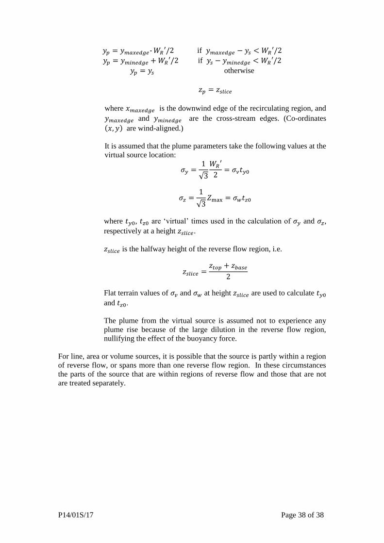
P14/01S/17 of 38

if

if

otherwise

where is the downwind edge of the recirculating region, and

and are the cross-stream edges. (Co-ordinates

are wind-aligned.)

It is assumed that the plume parameters take the following values at the

virtual source location:

where , are ‘virtual’ times used in the calculation of and ,

respectively at a height .

is the halfway height of the reverse flow region, i.e.

Flat terrain values of and at height are used to calculate

and .

The plume from the virtual source is assumed not to experience any

plume rise because of the large dilution in the reverse flow region,

nullifying the effect of the buoyancy force.

For line, area or volume sources, it is possible that the source is partly within a region

of reverse flow, or spans more than one reverse flow region. In these circumstances

the parts of the source that are within regions of reverse flow and those that are not

are treated separately.

complex terrain module€¦ · the adms complex terrain module models dispersion over hills and...

Documents