complete solutions manual - blog.kakaocdn.net
TRANSCRIPT

Complete Solutions Manual
Prepared by
Roger Lipsett
Australia • Brazil • Japan • Korea • Mexico • Singapore • Spain • United Kingdom • United States
Linear Algebra A Modern Introduction
FOURTH EDITION
David Poole Trent University

Printed in the United States of America 1 2 3 4 5 6 7 17 16 15 14 13
© 2015 Cengage Learning ALL RIGHTS RESERVED. No part of this work covered by the copyright herein may be reproduced, transmitted, stored, or used in any form or by any means graphic, electronic, or mechanical, including but not limited to photocopying, recording, scanning, digitizing, taping, Web distribution, information networks, or information storage and retrieval systems, except as permitted under Section 107 or 108 of the 1976 United States Copyright Act, without the prior written permission of the publisher except as may be permitted by the license terms below.
For product information and technology assistance, contact us at Cengage Learning Customer & Sales Support,
1-800-354-9706.
For permission to use material from this text or product, submit all requests online at www.cengage.com/permissions
Further permissions questions can be emailed to [email protected].
ISBN-13: 978-128586960-5 ISBN-10: 1-28586960-5 Cengage Learning 200 First Stamford Place, 4th Floor Stamford, CT 06902 USA Cengage Learning is a leading provider of customized learning solutions with office locations around the globe, including Singapore, the United Kingdom, Australia, Mexico, Brazil, and Japan. Locate your local office at: www.cengage.com/global. Cengage Learning products are represented in Canada by Nelson Education, Ltd. To learn more about Cengage Learning Solutions, visit www.cengage.com. Purchase any of our products at your local college store or at our preferred online store www.cengagebrain.com.
NOTE: UNDER NO CIRCUMSTANCES MAY THIS MATERIAL OR ANY PORTION THEREOF BE SOLD, LICENSED, AUCTIONED,
OR OTHERWISE REDISTRIBUTED EXCEPT AS MAY BE PERMITTED BY THE LICENSE TERMS HEREIN.
READ IMPORTANT LICENSE INFORMATION
Dear Professor or Other Supplement Recipient: Cengage Learning has provided you with this product (the “Supplement”) for your review and, to the extent that you adopt the associated textbook for use in connection with your course (the “Course”), you and your students who purchase the textbook may use the Supplement as described below. Cengage Learning has established these use limitations in response to concerns raised by authors, professors, and other users regarding the pedagogical problems stemming from unlimited distribution of Supplements. Cengage Learning hereby grants you a nontransferable license to use the Supplement in connection with the Course, subject to the following conditions. The Supplement is for your personal, noncommercial use only and may not be reproduced, posted electronically or distributed, except that portions of the Supplement may be provided to your students IN PRINT FORM ONLY in connection with your instruction of the Course, so long as such students are advised that they
may not copy or distribute any portion of the Supplement to any third party. You may not sell, license, auction, or otherwise redistribute the Supplement in any form. We ask that you take reasonable steps to protect the Supplement from unauthorized use, reproduction, or distribution. Your use of the Supplement indicates your acceptance of the conditions set forth in this Agreement. If you do not accept these conditions, you must return the Supplement unused within 30 days of receipt. All rights (including without limitation, copyrights, patents, and trade secrets) in the Supplement are and will remain the sole and exclusive property of Cengage Learning and/or its licensors. The Supplement is furnished by Cengage Learning on an “as is” basis without any warranties, express or implied. This Agreement will be governed by and construed pursuant to the laws of the State of New York, without regard to such State’s conflict of law rules. Thank you for your assistance in helping to safeguard the integrity of the content contained in this Supplement. We trust you find the Supplement a useful teaching tool.

Contents
1 Vectors 3
1.1 The Geometry and Algebra of Vectors . . . . . . . . . . . . . . . . . . . . . . . . . . . . . . . 3
1.2 Length and Angle: The Dot Product . . . . . . . . . . . . . . . . . . . . . . . . . . . . . . . . 10
Exploration: Vectors and Geometry . . . . . . . . . . . . . . . . . . . . . . . . . . . . . . . . . . . 25
1.3 Lines and Planes . . . . . . . . . . . . . . . . . . . . . . . . . . . . . . . . . . . . . . . . . . . 27
Exploration: The Cross Product . . . . . . . . . . . . . . . . . . . . . . . . . . . . . . . . . . . . . 41
1.4 Applications . . . . . . . . . . . . . . . . . . . . . . . . . . . . . . . . . . . . . . . . . . . . . . 44
Chapter Review . . . . . . . . . . . . . . . . . . . . . . . . . . . . . . . . . . . . . . . . . . . . . . . 48
2 Systems of Linear Equations 53
2.1 Introduction to Systems of Linear Equations . . . . . . . . . . . . . . . . . . . . . . . . . . . 53
2.2 Direct Methods for Solving Linear Systems . . . . . . . . . . . . . . . . . . . . . . . . . . . . 58
Exploration: Lies My Computer Told Me . . . . . . . . . . . . . . . . . . . . . . . . . . . . . . . . 75
Exploration: Partial Pivoting . . . . . . . . . . . . . . . . . . . . . . . . . . . . . . . . . . . . . . . 75
Exploration: An Introduction to the Analysis of Algorithms . . . . . . . . . . . . . . . . . . . . . . 77
2.3 Spanning Sets and Linear Independence . . . . . . . . . . . . . . . . . . . . . . . . . . . . . . 79
2.4 Applications . . . . . . . . . . . . . . . . . . . . . . . . . . . . . . . . . . . . . . . . . . . . . . 93
2.5 Iterative Methods for Solving Linear Systems . . . . . . . . . . . . . . . . . . . . . . . . . . . 112
Chapter Review . . . . . . . . . . . . . . . . . . . . . . . . . . . . . . . . . . . . . . . . . . . . . . . 123
3 Matrices 129
3.1 Matrix Operations . . . . . . . . . . . . . . . . . . . . . . . . . . . . . . . . . . . . . . . . . . 129
3.2 Matrix Algebra . . . . . . . . . . . . . . . . . . . . . . . . . . . . . . . . . . . . . . . . . . . . 138
3.3 The Inverse of a Matrix . . . . . . . . . . . . . . . . . . . . . . . . . . . . . . . . . . . . . . . 150
3.4 The LU Factorization . . . . . . . . . . . . . . . . . . . . . . . . . . . . . . . . . . . . . . . . 164
3.5 Subspaces, Basis, Dimension, and Rank . . . . . . . . . . . . . . . . . . . . . . . . . . . . . . 176
3.6 Introduction to Linear Transformations . . . . . . . . . . . . . . . . . . . . . . . . . . . . . . 192
3.7 Applications . . . . . . . . . . . . . . . . . . . . . . . . . . . . . . . . . . . . . . . . . . . . . . 209
Chapter Review . . . . . . . . . . . . . . . . . . . . . . . . . . . . . . . . . . . . . . . . . . . . . . . 230
4 Eigenvalues and Eigenvectors 235
4.1 Introduction to Eigenvalues and Eigenvectors . . . . . . . . . . . . . . . . . . . . . . . . . . . 235
4.2 Determinants . . . . . . . . . . . . . . . . . . . . . . . . . . . . . . . . . . . . . . . . . . . . . 250
Exploration: Geometric Applications of Determinants . . . . . . . . . . . . . . . . . . . . . . . . . 263
4.3 Eigenvalues and Eigenvectors of n× n Matrices . . . . . . . . . . . . . . . . . . . . . . . . . . 270
4.4 Similarity and Diagonalization . . . . . . . . . . . . . . . . . . . . . . . . . . . . . . . . . . . 291
4.5 Iterative Methods for Computing Eigenvalues . . . . . . . . . . . . . . . . . . . . . . . . . . . 308
4.6 Applications and the Perron-Frobenius Theorem . . . . . . . . . . . . . . . . . . . . . . . . . 326
Chapter Review . . . . . . . . . . . . . . . . . . . . . . . . . . . . . . . . . . . . . . . . . . . . . . . 365
1

2 CONTENTS
5 Orthogonality 3715.1 Orthogonality in Rn . . . . . . . . . . . . . . . . . . . . . . . . . . . . . . . . . . . . . . . . . 3715.2 Orthogonal Complements and Orthogonal Projections . . . . . . . . . . . . . . . . . . . . . . 3795.3 The Gram-Schmidt Process and the QR Factorization . . . . . . . . . . . . . . . . . . . . . . 388Exploration: The Modified QR Process . . . . . . . . . . . . . . . . . . . . . . . . . . . . . . . . . 398Exploration: Approximating Eigenvalues with the QR Algorithm . . . . . . . . . . . . . . . . . . . 4025.4 Orthogonal Diagonalization of Symmetric Matrices . . . . . . . . . . . . . . . . . . . . . . . . 4055.5 Applications . . . . . . . . . . . . . . . . . . . . . . . . . . . . . . . . . . . . . . . . . . . . . . 417Chapter Review . . . . . . . . . . . . . . . . . . . . . . . . . . . . . . . . . . . . . . . . . . . . . . . 442
6 Vector Spaces 4516.1 Vector Spaces and Subspaces . . . . . . . . . . . . . . . . . . . . . . . . . . . . . . . . . . . . 4516.2 Linear Independence, Basis, and Dimension . . . . . . . . . . . . . . . . . . . . . . . . . . . . 463Exploration: Magic Squares . . . . . . . . . . . . . . . . . . . . . . . . . . . . . . . . . . . . . . . . 4776.3 Change of Basis . . . . . . . . . . . . . . . . . . . . . . . . . . . . . . . . . . . . . . . . . . . . 4806.4 Linear Transformations . . . . . . . . . . . . . . . . . . . . . . . . . . . . . . . . . . . . . . . 4916.5 The Kernel and Range of a Linear Transformation . . . . . . . . . . . . . . . . . . . . . . . . 4986.6 The Matrix of a Linear Transformation . . . . . . . . . . . . . . . . . . . . . . . . . . . . . . 507Exploration: Tiles, Lattices, and the Crystallographic Restriction . . . . . . . . . . . . . . . . . . . 5256.7 Applications . . . . . . . . . . . . . . . . . . . . . . . . . . . . . . . . . . . . . . . . . . . . . . 527Chapter Review . . . . . . . . . . . . . . . . . . . . . . . . . . . . . . . . . . . . . . . . . . . . . . . 531
7 Distance and Approximation 5377.1 Inner Product Spaces . . . . . . . . . . . . . . . . . . . . . . . . . . . . . . . . . . . . . . . . . 537Exploration: Vectors and Matrices with Complex Entries . . . . . . . . . . . . . . . . . . . . . . . 546Exploration: Geometric Inequalities and Optimization Problems . . . . . . . . . . . . . . . . . . . 5537.2 Norms and Distance Functions . . . . . . . . . . . . . . . . . . . . . . . . . . . . . . . . . . . 5567.3 Least Squares Approximation . . . . . . . . . . . . . . . . . . . . . . . . . . . . . . . . . . . . 5687.4 The Singular Value Decomposition . . . . . . . . . . . . . . . . . . . . . . . . . . . . . . . . . 5907.5 Applications . . . . . . . . . . . . . . . . . . . . . . . . . . . . . . . . . . . . . . . . . . . . . . 614Chapter Review . . . . . . . . . . . . . . . . . . . . . . . . . . . . . . . . . . . . . . . . . . . . . . . 625
8 Codes 6338.1 Code Vectors . . . . . . . . . . . . . . . . . . . . . . . . . . . . . . . . . . . . . . . . . . . . . 6338.2 Error-Correcting Codes . . . . . . . . . . . . . . . . . . . . . . . . . . . . . . . . . . . . . . . 6378.3 Dual Codes . . . . . . . . . . . . . . . . . . . . . . . . . . . . . . . . . . . . . . . . . . . . . . 6418.4 Linear Codes . . . . . . . . . . . . . . . . . . . . . . . . . . . . . . . . . . . . . . . . . . . . . 6478.5 The Minimum Distance of a Code . . . . . . . . . . . . . . . . . . . . . . . . . . . . . . . . . 650
Chapter 1
Vectors
1.1 The Geometry and Algebra of Vectors
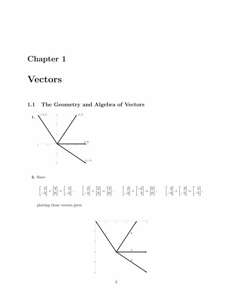
1.
H3, 0L
H2, 3L
H3, -2L
H-2, 3L
-2 -1 1 2 3
-2
-1
1
2
3
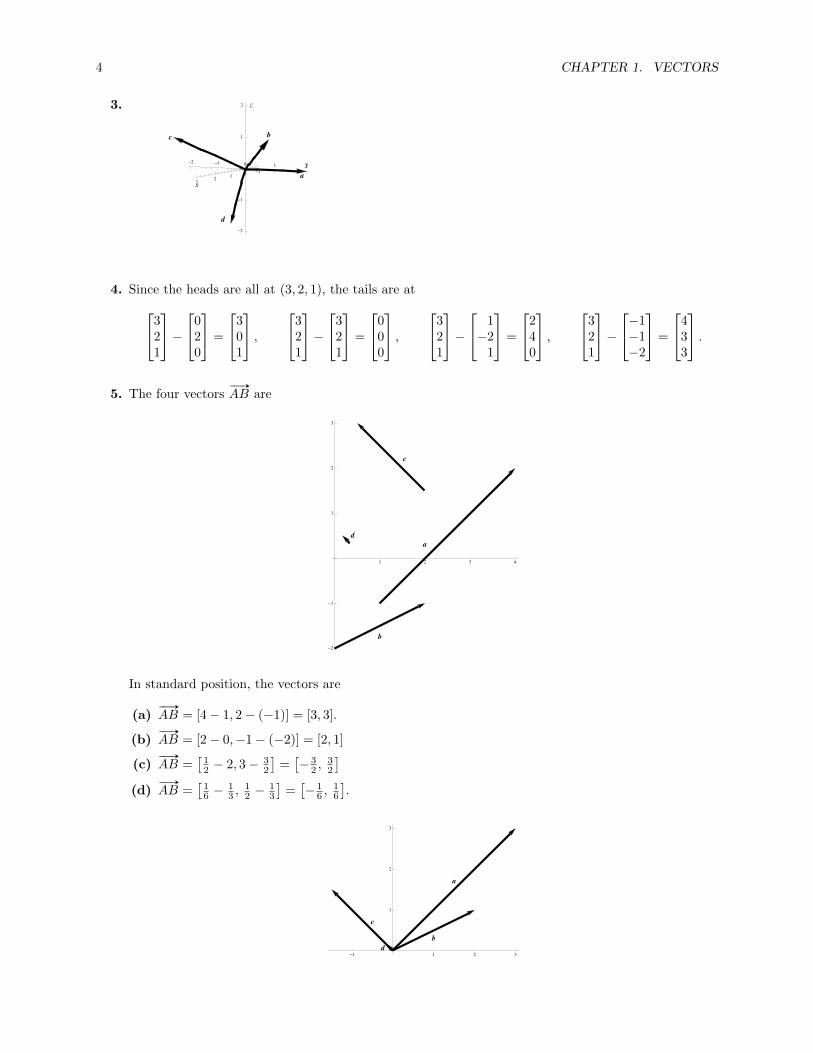
2. Since
[2−3
]+
[30
]=
[5−3
],
[2−3
]+
[23
]=
[40
],
[2−3
]+
[−2
3
]=
[00
],
[2−3
]+
[3−2
]=
[5−5
],
plotting those vectors gives
a
bc
d
1 2 3 4 5
-5
-4
-3
-2
-1
3
4 CHAPTER 1. VECTORS
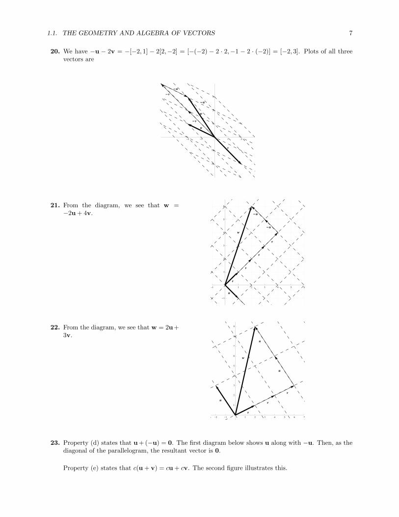
3.
a
bc
d
x
y
z
-10
12
3
-2-1 0 1 2
-2
-1
0
1
2
4. Since the heads are all at (3, 2, 1), the tails are at321
−0
20
=
301
,3
21
−3
21
=
000
,3
21
− 1−2
1
=
240
,3
21
−−1−1−2
=
433
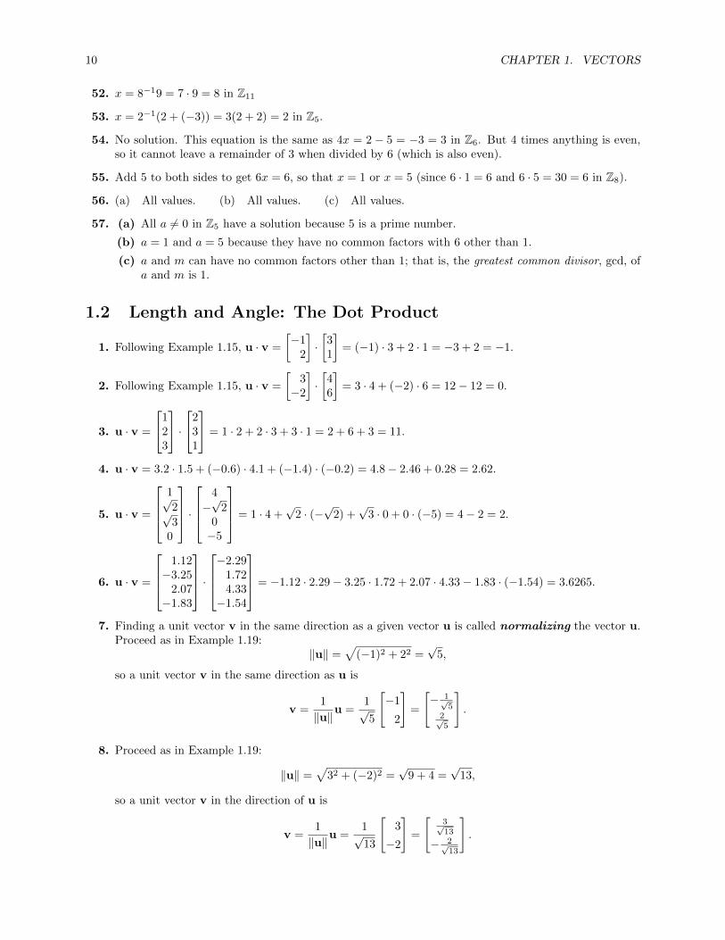
.5. The four vectors
# »
AB are
a
b
c
d
1 2 3 4
-2
-1
1
2
3
In standard position, the vectors are
(a)# »
AB = [4− 1, 2− (−1)] = [3, 3].
(b)# »
AB = [2− 0,−1− (−2)] = [2, 1]
(c)# »
AB =[
12 − 2, 3− 3
2
]=[− 3
2 ,32
](d)
# »
AB =[
16 −
13 ,
12 −
13
]=[− 1
6 ,16
].
a
b
c
d-1 1 2 3
1
2
3

1.1. THE GEOMETRY AND ALGEBRA OF VECTORS 5
6. Recall the notation that [a, b] denotes a move of a units horizontally and b units vertically. Then duringthe first part of the walk, the hiker walks 4 km north, so a = [0, 4]. During the second part of thewalk, the hiker walks a distance of 5 km northeast. From the components, we get
b = [5 cos 45◦, 5 sin 45◦] =
[5√
2
2,
5√
2
2
].
Thus the net displacement vector is
c = a + b =
[5√
2
2, 4 +
5√
2
2
].
7. a + b =
[30
]+
[23
]=
[3 + 20 + 3
]=
[53
].
a
b
a + b
1 2 3 4 5
1
2
3
8. b−c =
[23
]−[−2
3
]=
[2− (−2)
3− 3
]=
[40
].
b -c
b - c
1 2 3 4
1
2
3
9. d− c =
[3−2
]−[−2
3
]=
[5−5
].
d
-cd - c
1 2 3 4 5
-5
-4
-3
-2
-1
10. a + d =
[30
]+
[3−2
]=
[3 + 3
0 + (−2)
]=[
6−2
].
a
d
a + d
1 2 3 4 5 6
-2
-1
11. 2a + 3c = 2[0, 2, 0] + 3[1,−2, 1] = [2 · 0, 2 · 2, 2 · 0] + [3 · 1, 3 · (−2), 3 · 1] = [3,−2, 3].
12.
3b− 2c + d = 3[3, 2, 1]− 2[1,−2, 1] + [−1,−1,−2]
= [3 · 3, 3 · 2, 3 · 1] + [−2 · 1,−2 · (−2),−2 · 1] + [−1,−1,−2]
= [6, 9,−1].

6 CHAPTER 1. VECTORS
13. u = [cos 60◦, sin 60◦] =[
12 ,√
32
], and v = [cos 210◦, sin 210◦] =
[−√
32 , −
12
], so that
u + v =
[1
2−√
3
2,
√3
2− 1
2
], u− v =
[1
2+
√3
2,
√3
2+
1
2
].
14. (a)# »
AB = b− a.
(b) Since# »
OC =# »
AB, we have# »
BC =# »
OC − b = (b− a)− b = −a.
(c)# »
AD = −2a.
(d)# »
CF = −2# »
OC = −2# »
AB = −2(b− a) = 2(a− b).
(e)# »
AC =# »
AB +# »
BC = (b− a) + (−a) = b− 2a.
(f) Note that# »
FA and# »
OB are equal, and that# »
DE = − # »
AB. Then
# »
BC +# »
DE +# »
FA = −a− # »
AB +# »
OB = −a− (b− a) + b = 0.
15. 2(a− 3b) + 3(2b + a)
property e.distributivity
= (2a− 6b) + (6b + 3a)
property b.associativity
= (2a + 3a) + (−6b + 6b) = 5a.
16.
−3(a− c) + 2(a + 2b) + 3(c− b)
property e.distributivity
= (−3a + 3c) + (2a + 4b) + (3c− 3b)
property b.associativity
= (−3a + 2a) + (4b− 3b) + (3c + 3c)
= −a + b + 6c.
17. x− a = 2(x− 2a) = 2x− 4a⇒ x− 2x = a− 4a⇒ −x = −3a⇒ x = 3a.
18.
x + 2a− b = 3(x + a)− 2(2a− b) = 3x + 3a− 4a + 2b ⇒x− 3x = −a− 2a + 2b + b ⇒
−2x = −3a + 3b ⇒
x =3
2a− 3
2b.
19. We have 2u+ 3v = 2[1,−1] + 3[1, 1] = [2 · 1 + 3 · 1, 2 · (−1) + 3 · 1] = [5, 1]. Plots of all three vectors are
u
v
w
uv
v
v
-1 1 2 3 4 5 6
-2
-1
1
2
1.1. THE GEOMETRY AND ALGEBRA OF VECTORS 7
20. We have −u − 2v = −[−2, 1] − 2[2,−2] = [−(−2) − 2 · 2,−1 − 2 · (−2)] = [−2, 3]. Plots of all threevectors are
u
v
w
-v
-v
-u
-u
-2 -1 1 2
-2
-1
1
2
3
21. From the diagram, we see that w =−2u + 4v.
u
v
w
-u
-u
v
v
v
-1 1 2 3 4 5 6
-1
1
2
3
4
5
6
22. From the diagram, we see that w = 2u+3v.
u
u
u
v
v
v
w
-2 -1 1 2 3 4 5 6 7
1
2
3
4
5
6
7
8
9
23. Property (d) states that u+ (−u) = 0. The first diagram below shows u along with −u. Then, as thediagonal of the parallelogram, the resultant vector is 0.
Property (e) states that c(u + v) = cu + cv. The second figure illustrates this.

8 CHAPTER 1. VECTORS
u
-u
u
v
u
v
u + v
cu
cu
cv
cv
cHu + vL
24. Let u = [u1, u2, . . . , un] and v = [v1, v2, . . . , vn], and let c and d be scalars in R.
Property (d):
u + (−u) = [u1, u2, . . . , un] + (−1[u1, u2, . . . , un])
= [u1, u2, . . . , un] + [−u1,−u2, . . . ,−un]
= [u1 − u1, u2 − u2, . . . , un − un]
= [0, 0, . . . , 0] = 0.
Property (e):
c(u + v) = c ([u1, u2, . . . , un] + [v1, v2, . . . , vn])
= c ([u1 + v1, u2 + v2, . . . , un + vn])
= [c(u1 + v1), c(u2 + v2), . . . , c(un + vn)]
= [cu1 + cv1, cu2 + cv2, . . . , cun + cvn]
= [cu1, cu2, . . . , cun] + [cv1, cv2, . . . , cvn]
= c[u1, u2, . . . , un] + c[v1, v2, . . . , vn]
= cu + cv.
Property (f):
(c+ d)u = (c+ d)[u1, u2, . . . , un]
= [(c+ d)u1, (c+ d)u2, . . . , (c+ d)un]
= [cu1 + du1, cu2 + du2, . . . , cun + dun]
= [cu1, cu2, . . . , cun] + [du1, du2, . . . , dun]
= c[u1, u2, . . . , un] + d[u1, u2, . . . , un]
= cu + du.
Property (g):
c(du) = c(d[u1, u2, . . . , un])
= c[du1, du2, . . . , dun]
= [cdu1, cdu2, . . . , cdun]
= [(cd)u1, (cd)u2, . . . , (cd)un]
= (cd)[u1, u2, . . . , un]
= (cd)u.
25. u + v = [0, 1] + [1, 1] = [1, 0].
26. u + v = [1, 1, 0] + [1, 1, 1] = [0, 0, 1].

1.1. THE GEOMETRY AND ALGEBRA OF VECTORS 9
27. u + v = [1, 0, 1, 1] + [1, 1, 1, 1] = [0, 1, 0, 0].
28. u + v = [1, 1, 0, 1, 0] + [0, 1, 1, 1, 0] = [1, 0, 1, 0, 0].
29.+ 0 1 2 30 0 1 2 31 1 2 3 02 2 3 0 13 3 0 1 2
· 0 1 2 30 0 0 0 01 0 1 2 32 0 2 0 23 0 3 2 1
30.+ 0 1 2 3 40 0 1 2 3 41 1 2 3 4 02 2 3 4 0 13 3 4 0 1 24 4 0 1 2 3
· 0 1 2 3 40 0 0 0 0 01 0 1 2 3 42 0 2 4 1 33 0 3 1 4 24 0 4 3 2 1
31. 2 + 2 + 2 = 6 = 0 in Z3.
32. 2 · 2 · 2 = 3 · 2 = 0 in Z3.
33. 2(2 + 1 + 2) = 2 · 2 = 3 · 1 + 1 = 1 in Z3.
34. 3 + 1 + 2 + 3 = 4 · 2 + 1 = 1 in Z4.
35. 2 · 3 · 2 = 4 · 3 + 0 = 0 in Z4.
36. 3(3 + 3 + 2) = 4 · 6 + 0 = 0 in Z4.
37. 2 + 1 + 2 + 2 + 1 = 2 in Z3, 2 + 1 + 2 + 2 + 1 = 0 in Z4, 2 + 1 + 2 + 2 + 1 = 3 in Z5.
38. (3 + 4)(3 + 2 + 4 + 2) = 2 · 1 = 2 in Z5.
39. 8(6 + 4 + 3) = 8 · 4 = 5 in Z9.
40. 2100 =(210)10
= (1024)10 = 110 = 1 in Z11.
41. [2, 1, 2] + [2, 0, 1] = [1, 1, 0] in Z33.
42. 2[2, 2, 1] = [2 · 2, 2 · 2, 2 · 1] = [1, 1, 2] in Z33.
43. 2([3, 1, 1, 2] + [3, 3, 2, 1]) = 2[2, 0, 3, 3] = [2 · 2, 2 · 0, 2 · 3, 2 · 3] = [0, 0, 2, 2] in Z44.
2([3, 1, 1, 2] + [3, 3, 2, 1]) = 2[1, 4, 3, 3] = [2 · 1, 2 · 4, 2 · 3, 2 · 3] = [2, 3, 1, 1] in Z45.
44. x = 2 + (−3) = 2 + 2 = 4 in Z5.
45. x = 1 + (−5) = 1 + 1 = 2 in Z6
46. x = 2−1 = 2 in Z3.
47. No solution. 2 times anything is always even, so cannot leave a remainder of 1 when divided by 4.
48. x = 2−1 = 3 in Z5.
49. x = 3−14 = 2 · 4 = 3 in Z5.
50. No solution. 3 times anything is always a multiple of 3, so it cannot leave a remainder of 4 whendivided by 6 (which is also a multiple of 3).
51. No solution. 6 times anything is always even, so it cannot leave an odd number as a remainder whendivided by 8.
10 CHAPTER 1. VECTORS
52. x = 8−19 = 7 · 9 = 8 in Z11
53. x = 2−1(2 + (−3)) = 3(2 + 2) = 2 in Z5.
54. No solution. This equation is the same as 4x = 2 − 5 = −3 = 3 in Z6. But 4 times anything is even,so it cannot leave a remainder of 3 when divided by 6 (which is also even).
55. Add 5 to both sides to get 6x = 6, so that x = 1 or x = 5 (since 6 · 1 = 6 and 6 · 5 = 30 = 6 in Z8).
56. (a) All values. (b) All values. (c) All values.
57. (a) All a 6= 0 in Z5 have a solution because 5 is a prime number.
(b) a = 1 and a = 5 because they have no common factors with 6 other than 1.
(c) a and m can have no common factors other than 1; that is, the greatest common divisor, gcd, ofa and m is 1.
1.2 Length and Angle: The Dot Product
1. Following Example 1.15, u · v =
[−1
2
]·[31
]= (−1) · 3 + 2 · 1 = −3 + 2 = −1.
2. Following Example 1.15, u · v =
[3−2
]·[46
]= 3 · 4 + (−2) · 6 = 12− 12 = 0.
3. u · v =
123
·2
31
= 1 · 2 + 2 · 3 + 3 · 1 = 2 + 6 + 3 = 11.
4. u · v = 3.2 · 1.5 + (−0.6) · 4.1 + (−1.4) · (−0.2) = 4.8− 2.46 + 0.28 = 2.62.
5. u · v =
1√2√3
0
·
4
−√
20−5
= 1 · 4 +√
2 · (−√
2) +√
3 · 0 + 0 · (−5) = 4− 2 = 2.
6. u · v =
1.12−3.25
2.07−1.83
·−2.29
1.724.33−1.54
= −1.12 · 2.29− 3.25 · 1.72 + 2.07 · 4.33− 1.83 · (−1.54) = 3.6265.
7. Finding a unit vector v in the same direction as a given vector u is called normalizing the vector u.Proceed as in Example 1.19:
‖u‖ =√
(−1)2 + 22 =√
5,
so a unit vector v in the same direction as u is
v =1
‖u‖u =
1√5
[−1
2
]=
[− 1√
52√5
].
8. Proceed as in Example 1.19:
‖u‖ =√
32 + (−2)2 =√
9 + 4 =√
13,
so a unit vector v in the direction of u is
v =1
‖u‖u =
1√13
[3
−2
]=
[3√13
− 2√13
].

1.2. LENGTH AND ANGLE: THE DOT PRODUCT 11
9. Proceed as in Example 1.19:
‖u‖ =√
12 + 22 + 32 =√
14,
so a unit vector v in the direction of u is
v =1
‖u‖u =
1√14
1
2
3
=
1√142√143√14
.10. Proceed as in Example 1.19:
‖u‖ =√
3.22 + (−0.6)2 + (−1.4)2 =√
10.24 + 0.36 + 1.96 =√
12.56 ≈ 3.544,
so a unit vector v in the direction of u is
v =1
‖u‖u =
1
3.544
1.50.4−2.1
≈ 0.903−0.169−0.395
.11. Proceed as in Example 1.19:
‖u‖ =
√12 +
(√2)2
+(√
3)2
+ 02 =√
6,
so a unit vector v in the direction of u is
v =1
‖u‖u =
1√6
1√
2√
3
0
=
1√6√2√6√3√6
0
=
1√6
1√3
1√2
0
=
√
66√3
3√2
2
0
12. Proceed as in Example 1.19:
‖u‖ =√
1.122 + (−3.25)2 + 2.072 + (−1.83)2 =√
1.2544 + 10.5625 + 4.2849 + 3.3489
=√
19.4507 ≈ 4.410,
so a unit vector v in the direction of u is
v1
‖u‖u =
1
4.410
[1.12 −3.25 2.07 −1.83
]≈[0.254 −0.737 0.469 −0.415
].
13. Following Example 1.20, we compute: u− v =
[−1
2
]−[31
]=
[−4
1
], so
d(u,v) = ‖u− v‖ =
√(−4)
2+ 12 =
√17.
14. Following Example 1.20, we compute: u− v =
[3−2
]−[46
]=
[−1−8
], so
d(u,v) = ‖u− v‖ =
√(−1)
2+ (−8)
2=√
65.
15. Following Example 1.20, we compute: u− v =
123
−2
31
=
−1−1
2
, so
d(u,v) = ‖u− v‖ =
√(−1)
2+ (−1)
2+ 22 =
√6.

12 CHAPTER 1. VECTORS
16. Following Example 1.20, we compute: u− v =
3.2−0.6−1.4
− 1.5
4.1−0.2
=
1.7−4.7−1.2
, so
d(u,v) = ‖u− v‖ =√
1.72 + (−4.7)2 + (−1.2)2 =√
26.42 ≈ 5.14.
17. (a) u · v is a real number, so ‖u · v‖ is the norm of a number, which is not defined.
(b) u · v is a scalar, while w is a vector. Thus u · v + w adds a scalar to a vector, which is not adefined operation.
(c) u is a vector, while v ·w is a scalar. Thus u · (v ·w) is the dot product of a vector and a scalar,which is not defined.
(d) c · (u + v) is the dot product of a scalar and a vector, which is not defined.
18. Let θ be the angle between u and v. Then
cos θ =u · v‖u‖ ‖v‖
=3 · (−1) + 0 · 1√
32 + 02√
(−1)2 + 12= − 3
3√
2= −√
2
2.
Thus cos θ < 0 (in fact, θ = 3π4 ), so the angle between u and v is obtuse.
19. Let θ be the angle between u and v. Then
cos θ =u · v‖u‖ ‖v‖
=2 · 1 + (−1) · (−2) + 1 · (−1)√
22 + (−1)2 + 12√
12 + (−2)2 + 12=
1
2.
Thus cos θ > 0 (in fact, θ = π3 ), so the angle between u and v is acute.
20. Let θ be the angle between u and v. Then
cos θ =u · v‖u‖ ‖v‖
=4 · 1 + 3 · (−1) + (−1) · 1√
42 + 32 + (−1)2√
12 + (−1)2 + 12=
0√26√
3= 0.
Thus the angle between u and v is a right angle.
21. Let θ be the angle between u and v. Note that we can determine whether θ is acute, right, or obtuseby examining the sign of u·v
‖u‖‖v‖ , which is determined by the sign of u · v. Since
u · v = 0.9 · (−4.5) + 2.1 · 2.6 + 1.2 · (−0.8) = 0.45 > 0,
we have cos θ > 0 so that θ is acute.
22. Let θ be the angle between u and v. Note that we can determine whether θ is acute, right, or obtuseby examining the sign of u·v
‖u‖‖v‖ , which is determined by the sign of u · v. Since
u · v = 1 · (−3) + 2 · 1 + 3 · 2 + 4 · (−2) = −3,
we have cos θ < 0 so that θ is obtuse.
23. Since the components of both u and v are positive, it is clear that u · v > 0, so the angle betweenthem is acute since it has a positive cosine.
24. From Exercise 18, cos θ = −√
22 , so that θ = cos−1
(−√
22
)= 3π
4 = 135◦.
25. From Exercise 19, cos θ = 12 , so that θ = cos−1 1
2 = π3 = 60◦.
26. From Exercise 20, cos θ = 0, so that θ = π2 = 90◦ is a right angle.

1.2. LENGTH AND ANGLE: THE DOT PRODUCT 13
27. As in Example 1.21, we begin by calculating u · v and the norms of the two vectors:
u · v = 0.9 · (−4.5) + 2.1 · 2.6 + 1.2 · (−0.8) = 0.45,
‖u‖ =√
0.92 + 2.12 + 1.22 =√
6.66,
‖v‖ =√
(−4.5)2 + 2.62 + (−0.8)2 =√
27.65.
So if θ is the angle between u and v, then
cos θ =u · v‖u‖ ‖v‖
=0.45√
6.66√
27.65≈ 0.45√
182.817,
so that
θ = cos−1
(0.45√
182.817
)≈ 1.5375 ≈ 88.09◦.
Note that it is important to maintain as much precision as possible until the last step, or roundofferrors may build up.
28. As in Example 1.21, we begin by calculating u · v and the norms of the two vectors:
u · v = 1 · (−3) + 2 · 1 + 3 · 2 + 4 · (−2) = −3,
‖u‖ =√
12 + 22 + 32 + 42 =√
30,
‖v‖ =√
(−3)2 + 12 + 22 + (−2)2 =√
18.
So if θ is the angle between u and v, then
cos θ =u · v‖u‖ ‖v‖
= − 3√30√
18= − 1
2√
15so that θ = cos−1
(− 1
2√
15
)≈ 1.7 ≈ 97.42◦.
29. As in Example 1.21, we begin by calculating u · v and the norms of the two vectors:
u · v = 1 · 5 + 2 · 6 + 3 · 7 + 4 · 8 = 70,
‖u‖ =√
12 + 22 + 32 + 42 =√
30,
‖v‖ =√
52 + 62 + 72 + 82 =√
174.
So if θ is the angle between u and v, then
cos θ =u · v‖u‖ ‖v‖
=70√
30√
174=
35
3√
145so that θ = cos−1
(35
3√
145
)≈ 0.2502 ≈ 14.34◦.
30. To show that 4ABC is right, we need only show that one pair of its sides meets at a right angle. Solet u =
# »
AB, v =# »
BC, and w =# »
AC. Then we must show that one of u · v, u ·w or v ·w is zero inorder to show that one of these pairs is orthogonal. Then
u =# »
AB = [1− (−3), 0− 2] = [4,−2] , v =# »
BC = [4− 1, 6− 0] = [3, 6] ,
w =# »
AC = [4− (−3), 6− 2] = [7, 4] ,
and
u · v = 4 · 3 + (−2) · 6 = 12− 12 = 0.
Since this dot product is zero, these two vectors are orthogonal, so that# »
AB ⊥ # »
BC and thus 4ABC isa right triangle. It is unnecessary to test the remaining pairs of sides.
14 CHAPTER 1. VECTORS
31. To show that 4ABC is right, we need only show that one pair of its sides meets at a right angle. Solet u =
# »
AB, v =# »
BC, and w =# »
AC. Then we must show that one of u · v, u ·w or v ·w is zero inorder to show that one of these pairs is orthogonal. Then
u =# »
AB = [−3− 1, 2− 1, (−2)− (−1)] = [−4, 1,−1] ,
v =# »
BC = [2− (−3), 2− 2, −4− (−2)] = [5, 0,−2],
w =# »
AC = [2− 1, 2− 1, −4− (−1)] = [1, 1,−3],
and
u · v = −4 · 5 + 1 · 0− 1 · (−2) = −18
u ·w = −4 · 1 + 1 · 1− 1 · (−3) = 0.
Since this dot product is zero, these two vectors are orthogonal, so that# »
AB ⊥ # »
AC and thus 4ABC isa right triangle. It is unnecessary to test the remaining pair of sides.
32. As in Example 1.22, the dimensions of the cube do not matter, so we work with a cube with side length1. Since the cube is symmetric, we need only consider one diagonal and adjacent edge. Orient the cubeas shown in Figure 1.34; take the diagonal to be [1, 1, 1] and the adjacent edge to be [1, 0, 0]. Then theangle θ between these two vectors satisfies
cos θ =1 · 1 + 1 · 0 + 1 · 0√
3√
1=
1√3, so θ = cos−1
(1√3
)≈ 54.74◦.
Thus the diagonal and an adjacent edge meet at an angle of 54.74◦.
33. As in Example 1.22, the dimensions of the cube do not matter, so we work with a cube with side length1. Since the cube is symmetric, we need only consider one pair of diagonals. Orient the cube as shownin Figure 1.34; take the diagonals to be u = [1, 1, 1] and v = [1, 1, 0] − [0, 0, 1] = [1, 1,−1]. Then thedot product is
u · v = 1 · 1 + 1 · 1 + 1 · (−1) = 1 + 1− 1 = 1 6= 0.
Since the dot product is nonzero, the diagonals are not orthogonal.
34. To show a parallelogram is a rhombus, it suffices to show that its diagonals are perpendicular (Euclid).But
d1 · d2 =
220
· 1−1
3
= 2 · 1 + 2 · (−1) + 0 · 3 = 0.
To determine its side length, note that since the diagonals are perpendicular, one half of each diagonalare the legs of a right triangle whose hypotenuse is one side of the rhombus. So we can use thePythagorean Theorem. Since
‖d1‖2 = 22 + 22 + 02 = 8, ‖d2‖2 = 12 + (−1)2 + 32 = 11,
we have for the side length
s2 =
(‖d1‖
2
)2
+
(‖d2‖
2
)2
=8
4+
11
4=
19
4,
so that s =√
192 ≈ 2.18.
35. Since ABCD is a rectangle, opposite sides BA and CD are parallel and congruent. So we can usethe method of Example 1.1 in Section 1.1 to find the coordinates of vertex D: we compute
# »
BA =[1− 3, 2− 6, 3− (−2)] = [−2,−4, 5]. If
# »
BA is then translated to# »
CD, where C = (0, 5,−4), then
D = (0 + (−2), 5 + (−4), −4 + 5) = (−2, 1, 1).

1.2. LENGTH AND ANGLE: THE DOT PRODUCT 15
36. The resultant velocity of the airplane is the sum of the velocity of the airplane and the velocity of thewind:
r = p + w =
[2000
]+
[0
−40
]=
[200−40
].
37. Let the x direction be east, in the direction of the current, and the y direction be north, across theriver. The speed of the boat is 4 mph north, and the current is 3 mph east, so the velocity of the boatis
v =
[04
]+
[30
]=
[34
].
38. Let the x direction be the direction across the river, and the y direction be downstream. Since vt = d,use the given information to find v, then solve for t and compute d. Since the speed of the boat is 20
km/h and the speed of the current is 5 km/h, we have v =
[205
]. The width of the river is 2 km, and
the distance downstream is unknown; call it y. Then d =
[2y
]. Thus
vt =
[205
]t =
[2y
].
Thus 20t = 2 so that t = 0.1, and then y = 5 · 0.1 = 0.5. Therefore
(a) Ann lands 0.5 km, or half a kilometer, downstream;
(b) It takes Ann 0.1 hours, or six minutes, to cross the river.
Note that the river flow does not increase the time required to cross the river, since its velocity isperpendicular to the direction of travel.
39. We want to find the angle between Bert’s resultant vector, r, and his velocity vector upstream, v. Letthe first coordinate of the vector be the direction across the river, and the second be the direction
upstream. Bert’s velocity vector directly across the river is unknown, say u =
[x0
]. His velocity vector
upstream compensates for the downstream flow, so v =
[01
]. So the resultant vector is r = u + v =[
x0
]+
[01
]=
[x1
]. Since Bert’s speed is 2 mph, we have ‖r‖ = 2. Thus
x2 + 1 = ‖r‖2 = 4, so that x =√
3.
If θ is the angle between r and v, then
cos θ =r · v‖r‖ ‖v‖
=
√3
2, so that θ = cos−1
(√3
2
)= 60◦.
40. We have
proju v =u · vu · u
u =(−1) · (−2) + 1 · 4(−1) · (−1) + 1 · 1
[−1
1
]= 3
[−1
1
]=
[−3
3
].
A graph of the situation is (with proju v in gray, and the perpendicular from v to the projection alsodrawn)

16 CHAPTER 1. VECTORS
u
v
projuHvL
-3 -2 -1
1
2
3
4
41. We have
proju v =u · vu · u
u =35 · 1 +
(− 4
5 · 2)
35 ·
35 +
(− 4
5
)·(− 4
5
) [ 35
− 45
]= −1
1u = −u.
A graph of the situation is (with proju v in gray, and the perpendicular from v to the projection alsodrawn)
u
v
projuHvL
1
1
2
42. We have
proju v =u · vu · u
u =12 · 2−
14 · 2−
12 · (−2)
12 ·
12 +
(− 1
4
) (− 1
4
)+(− 1
2
) (− 1
2
)
12
− 14
− 12
=8
3
12
− 14
− 12
=
43
− 23
− 43
.43. We have
proju v =u · vu · u
u =1 · 2 + (−1) · (−3) + 1 · (−1) + (−1) · (−2)
1 · 1 + (−1) · (−1) + 1 · 1 + (−1) · (−1)
1
−1
1
−1
=6
4
1
−1
1
−1
=
32
− 3232
− 32
=3
2u.
44. We have
proju v =u · vu · u
u =0.5 · 2.1 + 1.5 · 1.20.5 · 0.5 + 1.5 · 1.5
[0.51.5
]=
2.85
2.5
[0.51.5
]=
[0.571.71
]= 1.14u.

1.2. LENGTH AND ANGLE: THE DOT PRODUCT 17
45. We have
proju v =u · vu · u
u =3.01 · 1.34− 0.33 · 4.25 + 2.52 · (−1.66)
3.01 · 3.01− 0.33 · (−0.33) + 2.52 · 2.52
3.01−0.33
2.52
= − 1.5523
15.5194
3.01−0.33
2.52
≈−0.301
0.033−0.252
≈ − 1
10u.
46. Let u =# »
AB =
[2− 1
2− (−1)
]=
[13
]and v =
# »
AC =
[4− 1
0− (−1)
]=
[31
].
(a) To compute the projection, we need
u · v =
[13
]·[31
]= 6, u · u =
[13
]·[13
]= 10.
Thus
proju v =u · vu · u
u =3
5
[1
3
]=
[3595
],
so that
v − proju v =
[3
1
]−
[3595
]=
[125
− 45
].
Then
‖u‖ =√
12 + 32 =√
10, ‖v − proju v‖ =
√(12
5
)2
+
(4
5
)2
=4√
10
5,
so that finally
A =1
2‖u‖ ‖v − proju v‖ =
1
2
√10 · 4
√10
5= 4.
(b) We already know u · v = 6 and ‖u‖ =√
10 from part (a). Also, ‖v‖ =√
32 + 12 =√
10. So
cos θ =u · v‖u‖ ‖v‖
=6√
10√
10=
3
5,
so that
sin θ =√
1− cos2 θ =
√1−
(3
5
)2
=4
5.
Thus
A =1
2‖u‖ ‖v‖ sin θ =
1
2
√10√
10 · 4
5= 4.
47. Let u =# »
AB =
4− 3−2− (−1)
6− 4
=
1−1
2
and v =# »
AC =
5− 30− (−1)
2− 4
=
21−2
.
(a) To compute the projection, we need
u · v =
1−1
2
· 2
1−2
= −3, u · u =
1−1
2
· 1−1
2
= 6.
Thus
proju v =u · vu · u
u = −3
6
1
−1
2
=
−1212
−1
,
18 CHAPTER 1. VECTORS
so that
v − proju v =
2
1
−2
−−
12
12
−1
=
5212
−1
Then
‖u‖ =√
12 + (−1)2 + 22 =√
6, ‖v − proju v‖ =
√(5
2
)2
+
(1
2
)2
+ (−1)2 =
√30
2,
so that finally
A =1
2‖u‖ ‖v − proju v‖ =
1
2
√6 ·√
30
2=
3√
5
2.
(b) We already know u · v = −3 and ‖u‖ =√
6 from part (a). Also, ‖v‖ =√
22 + 12 + (−2)2 = 3.So
cos θ =u · v‖u‖ ‖v‖
=−3
3√
6= −√
6
6,
so that
sin θ =√
1− cos2 θ =
√√√√1−
(√6
6
)2
=
√30
6.
Thus
A =1
2‖u‖ ‖v‖ sin θ =
1
2
√6 · 3 ·
√30
6=
3√
5
2.
48. Two vectors u and v are orthogonal if and only if their dot product u · v = 0. So we set u · v = 0 andsolve for k:
u · v =
[23
]·[k + 1k − 1
]= 0 ⇒ 2(k + 1) + 3(k − 1) = 0 ⇒ 5k − 1 = 0 ⇒ k =
1
5.
Substituting into the formula for v gives
v =
[15 + 115 − 1
]=
[65
− 45
].
As a check, we compute
u · v =
[2
3
]·
[65
− 45
]=
12
5− 12
5= 0,
and the vectors are indeed orthogonal.
49. Two vectors u and v are orthogonal if and only if their dot product u · v = 0. So we set u · v = 0 andsolve for k:
u · v =
1−1
2
·k2
k−3
= 0 ⇒ k2 − k − 6 = 0 ⇒ (k + 2)(k − 3) = 0 ⇒ k = 2,−3.
Substituting into the formula for v gives
k = 2 : v1 =
(−2)2
−2−3
=
4−2−3
, k = −3 : v2 =
32
3−3
=
93−3
.As a check, we compute
u ·v1 =
1−1
2
· 4−2−3
= 1 · 4− 1 · (−2) + 2 · (−3) = 0, u ·v2 =
1−1
2
· 9
3−3
= 1 · 9− 1 · 3 + 2 · (−3) = 0
and the vectors are indeed orthogonal.

1.2. LENGTH AND ANGLE: THE DOT PRODUCT 19
50. Two vectors u and v are orthogonal if and only if their dot product u · v = 0. So we set u · v = 0 andsolve for y in terms of x:
u · v =
[31
]·[xy
]= 0 ⇒ 3x+ y = 0 ⇒ y = −3x.
Substituting y = −3x back into the formula for v gives
v =
[x−3x
]= x
[1−3
].
Thus any vector orthogonal to
[31
]is a multiple of
[1−3
]. As a check,
u · v =
[31
]·[x−3x
]= 3x− 3x = 0 for any value of x,
so that the vectors are indeed orthogonal.
51. As noted in the remarks just prior to Example 1.16, the zero vector 0 is orthogonal to all vectors in
R2. So if
[ab
]= 0, any vector
[xy
]will do. Now assume that
[ab
]6= 0; that is, that either a or b is
nonzero. Two vectors u and v are orthogonal if and only if their dot product u · v = 0. So we setu · v = 0 and solve for y in terms of x:
u · v =
[ab
]·[xy
]= 0 ⇒ ax+ by = 0.
First assume b 6= 0. Then y = −abx, so substituting back into the expression for v we get
v =
[x
−abx
]= x
[1
−ab
]=x
b
[b
−a
].
Next, if b = 0, then a 6= 0, so that x = − bay, and substituting back into the expression for v gives
v =
[− bay
y
]= y
[− ba
1
]= −y
a
[b
−a
].
So in either case, a vector orthogonal to
[ab
], if it is not the zero vector, is a multiple of
[b−a
]. As a
check, note that [ab
]·[
rb−ra
]= rab− rab = 0 for all values of r.
52. (a) The geometry of the vectors in Figure 1.26 suggests that if ‖u + v‖ = ‖u‖ + ‖v‖, then u and vpoint in the same direction. This means that the angle between them must be 0. So we first prove
Lemma 1. For all vectors u and v in R2 or R3, u · v = ‖u‖ ‖v‖ if and only if the vectors pointin the same direction.
Proof. Let θ be the angle between u and v. Then
cos θ =u · v‖u‖ ‖v‖
,
so that cos θ = 1 if and only if u · v = ‖u‖ ‖v‖. But cos θ = 1 if and only if θ = 0, which meansthat u and v point in the same direction.
20 CHAPTER 1. VECTORS
We can now show
Theorem 2. For all vectors u and v in R2 or R3, ‖u + v‖ = ‖u‖+ ‖v‖ if and only if u and vpoint in the same direction.
Proof. First assume that u and v point in the same direction. Then u · v = ‖u‖ ‖v‖, and thus
‖u + v‖2 =u · u + 2u · v + v · v By Example 1.9
= ‖u‖2 + 2u · v + ‖v‖2 Since w ·w = ‖w‖2 for any vector w
= ‖u‖2 + 2 ‖u‖ ‖v‖+ ‖v‖2 By the lemma
= (‖u‖+ ‖v‖)2.
Since ‖u + v‖ and ‖u‖+‖v‖ are both nonnegative, taking square roots gives ‖u + v‖ = ‖u‖+‖v‖.For the other direction, if ‖u + v‖ = ‖u‖+ ‖v‖, then their squares are equal, so that
(‖u‖+ ‖v‖)2= ‖u‖2 + 2 ‖u‖ ‖v‖+ ‖v‖2 and
‖u + v‖2 = u · u + 2u · v + v · v
are equal. But ‖u‖2 = u · u and similarly for v, so that canceling those terms gives 2u · v =2 ‖u‖ ‖v‖ and thus u ·v = ‖u‖ ‖v‖. Using the lemma again shows that u and v point in the samedirection.
(b) The geometry of the vectors in Figure 1.26 suggests that if ‖u + v‖ = ‖u‖ − ‖v‖, then u and vpoint in opposite directions. In addition, since ‖u + v‖ ≥ 0, we must also have ‖u‖ ≥ ‖v‖. Ifthey point in opposite directions, the angle between them must be π. This entire proof is exactlyanalogous to the proof in part (a). We first prove
Lemma 3. For all vectors u and v in R2 or R3, u ·v = −‖u‖ ‖v‖ if and only if the vectors pointin opposite directions.
Proof. Let θ be the angle between u and v. Then
cos θ =u · v‖u‖ ‖v‖
,
so that cos θ = −1 if and only if u · v = −‖u‖ ‖v‖. But cos θ = −1 if and only if θ = π, whichmeans that u and v point in opposite directions.
We can now show
Theorem 4. For all vectors u and v in R2 or R3, ‖u + v‖ = ‖u‖ − ‖v‖ if and only if u and vpoint in opposite directions and ‖u‖ ≥ ‖v‖.
Proof. First assume that u and v point in opposite directions and ‖u‖ ≥ ‖v‖. Then u · v =−‖u‖ ‖v‖, and thus
‖u + v‖2 =u · u + 2u · v + v · v By Example 1.9
= ‖u‖2 + 2u · v + ‖v‖2 Since w ·w = ‖w‖2 for any vector w
= ‖u‖2 − 2 ‖u‖ ‖v‖+ ‖v‖2 By the lemma
= (‖u‖ − ‖v‖)2.
Now, since ‖u‖ ≥ ‖v‖ by assumption, we see that both ‖u + v‖ and ‖u‖ − ‖v‖ are nonnegative,so that taking square roots gives ‖u + v‖ = ‖u‖ − ‖v‖. For the other direction, if ‖u + v‖ =
1.2. LENGTH AND ANGLE: THE DOT PRODUCT 21
‖u‖ − ‖v‖, then first of all, since the left-hand side is nonnegative, the right-hand side must beas well, so that ‖u‖ ≥ ‖v‖. Next, we can square both sides of the equality, so that
(‖u‖ − ‖v‖)2= ‖u‖2 − 2 ‖u‖ ‖v‖+ ‖v‖2 and
‖u + v‖2 = u · u + 2u · v + v · v
are equal. But ‖u‖2 = u · u and similarly for v, so that canceling those terms gives 2u · v =−2 ‖u‖ ‖v‖ and thus u · v = −‖u‖ ‖v‖. Using the lemma again shows that u and v point inopposite directions.
53. Prove Theorem 1.2(b) by applying the definition of the dot product:
u · v = u1(v1 + w1) + u2(v2 + w2) + · · ·+ un(vn + wn)
= u1v1 + u1w1 + u2v2 + u2w2 + · · ·+ unvn + unwn
= (u1v1 + u2v2 + · · ·+ unvn) + (u1w1 + u2w2 + · · ·+ unwn)
= u · v + u ·w.
54. Prove the three parts of Theorem 1.2(d) by applying the definition of the dot product and variousproperties of real numbers:
Part 1: For any vector u, we must show u · u ≥ 0. But
u · u = u1u1 + u2u2 + · · ·+ unun = u21 + u2
2 + · · ·+ u2n.
Since for any real number x we know that x2 ≥ 0, it follows that this sum is also nonnegative, sothat u · u ≥ 0.
Part 2: We must show that if u = 0 then u · u = 0. But u = 0 means that ui = 0 for all i, so that
u · u = 0 · 0 + 0 · 0 + · · ·+ 0 · 0 = 0.
Part 3: We must show that if u · u = 0, then u = 0. From part 1, we know that
u · u = u21 + u2
2 + · · ·+ u2n,
and that u2i ≥ 0 for all i. So if the dot product is to be zero, each u2
i must be zero, which meansthat ui = 0 for all i and thus u = 0.
55. We must show d(u,v) = ‖u− v‖ = ‖v − u‖ = d(v,u). By definition, d(u,v) = ‖u− v‖. Then byTheorem 1.3(b) with c = −1, we have ‖−w‖ = ‖w‖ for any vector w; applying this to the vector u−vgives
‖u− v‖ = ‖−(u− v)‖ = ‖v − u‖ ,which is by definition equal to d(v,u).
56. We must show that for any vectors u, v and w that d(u,w) ≤ d(u,v) + d(v,w). This is equivalent toshowing that ‖u−w‖ ≤ ‖u− v‖+ ‖v −w‖. Now substitute u− v for x and v−w for y in Theorem1.5, giving
‖u−w‖ = ‖(u− v) + (v −w)‖ ≤ ‖u− v‖+ ‖v −w‖ .
57. We must show that d(u,v) = ‖u− v‖ = 0 if and only if u = v. This follows immediately fromTheorem 1.3(a), ‖w‖ = 0 if and only if w = 0, upon setting w = u− v.
58. Apply the definitions:
u · cv = [u1, u2, . . . , un] · [cv1, cv2, . . . , cvn]
= u1cv1 + u2cv2 + · · ·+ uncvn
= cu1v1 + cu2v2 + · · ·+ cunvn
= c(u1v1 + u2v2 + · · ·+ unvn)
= c(u · v).

22 CHAPTER 1. VECTORS
59. We want to show that ‖u− v‖ ≥ ‖u‖− ‖v‖. This is equivalent to showing that ‖u‖ ≤ ‖u− v‖+ ‖v‖.This follows immediately upon setting x = u− v and y = v in Theorem 1.5.
60. If u · v = u ·w, it does not follow that v = w. For example, since 0 · v = 0 for every vector v in Rn,the zero vector is orthogonal to every vector v. So if u = 0 in the above equality, we know nothingabout v and w. (as an example, 0 · [1, 2] = 0 · [−17, 12]). Note, however, that u · v = u · w impliesthat u · v − u ·w = u(v −w) = 0, so that u is orthogonal to v −w.
61. We must show that (u + v)(u− v) = ‖u‖2 − ‖v‖2 for all vectors in Rn. Recall that for any w in Rnthat w ·w = ‖w‖2, and also that u · v = v · u. Then
(u + v)(u− v) = u · u + v · u− u · v − v · v = ‖u‖2 + u · v − u · v − ‖v‖2 = ‖u‖2 − ‖v‖2 .
62. (a) Let u,v ∈ Rn. Then
‖u + v‖2 + ‖u− v‖2 = (u + v) · (u + v) + (u− v) · (u− v)
= (u · u + v · v + 2u · v) + (u · u + v · v − 2u · v)
=(‖u‖2 + ‖v‖2
)+ 2u · v +
(‖u‖2 + ‖v‖2
)− 2u · v
= 2 ‖u‖2 + 2 ‖v‖2 .
(b) Part (a) tells us that the sum of thesquares of the lengths of the diagonalsof a parallelogram is equal to the sumof the squares of the lengths of its foursides.
u
v
u - v
u + v
63. Let u,v ∈ Rn. Then
1
4‖u + v‖2 − 1
4‖u− v‖2 =
1
4[(u + v) · (u + v)− ((u− v) · (u− v)]
=1
4[(u · u + v · v + 2u · v)− (u · u + v · v − 2u · v)]
=1
4
[(‖u‖2 − ‖u‖2
)+(‖v‖2 − ‖v‖2
)+ 4u · v
]= u · v.
64. (a) Let u,v ∈ Rn. Then using the previous exercise,
‖u + v‖ = ‖u− v‖ ⇔ ‖u + v‖2 = ‖u− v‖2
⇔ ‖u + v‖2 − ‖u− v‖2 = 0
⇔ 1
4‖u + v‖2 − 1
4‖u− v‖2 = 0
⇔ u · v = 0
⇔ u and v are orthogonal.
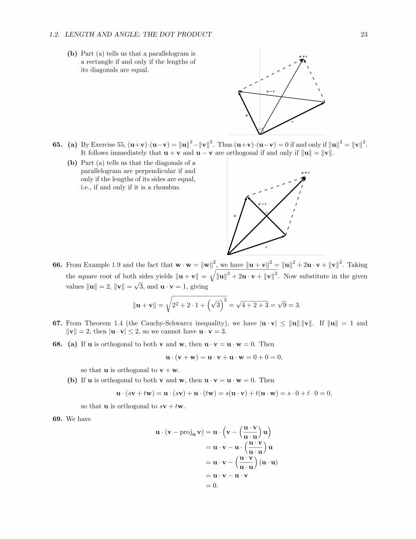
1.2. LENGTH AND ANGLE: THE DOT PRODUCT 23
(b) Part (a) tells us that a parallelogram isa rectangle if and only if the lengths ofits diagonals are equal.
u
v
u - v
u + v
65. (a) By Exercise 55, (u+v)·(u−v) = ‖u‖2−‖v‖2. Thus (u+v)·(u−v) = 0 if and only if ‖u‖2 = ‖v‖2.It follows immediately that u + v and u− v are orthogonal if and only if ‖u‖ = ‖v‖.
(b) Part (a) tells us that the diagonals of aparallelogram are perpendicular if andonly if the lengths of its sides are equal,i.e., if and only if it is a rhombus.
u
v
u - v
u + v
66. From Example 1.9 and the fact that w ·w = ‖w‖2, we have ‖u + v‖2 = ‖u‖2 + 2u · v + ‖v‖2. Taking
the square root of both sides yields ‖u + v‖ =
√‖u‖2 + 2u · v + ‖v‖2. Now substitute in the given
values ‖u‖ = 2, ‖v‖ =√
3, and u · v = 1, giving
‖u + v‖ =
√22 + 2 · 1 +
(√3)2
=√
4 + 2 + 3 =√
9 = 3.
67. From Theorem 1.4 (the Cauchy-Schwarcz inequality), we have |u · v| ≤ ‖u‖ ‖v‖. If ‖u‖ = 1 and‖v‖ = 2, then |u · v| ≤ 2, so we cannot have u · v = 3.
68. (a) If u is orthogonal to both v and w, then u · v = u ·w = 0. Then
u · (v + w) = u · v + u ·w = 0 + 0 = 0,
so that u is orthogonal to v + w.
(b) If u is orthogonal to both v and w, then u · v = u ·w = 0. Then
u · (sv + tw) = u · (sv) + u · (tw) = s(u · v) + t(u ·w) = s · 0 + t · 0 = 0,
so that u is orthogonal to sv + tw.
69. We have
u · (v − proju v) = u ·(v −
(u · vu · u
)u)
= u · v − u ·(u · vu · u
)u
= u · v −(u · vu · u
)(u · u)
= u · v − u · v= 0.

24 CHAPTER 1. VECTORS
70. (a) proju(proju v) = proju(u·vu·uu
)= u·v
u·u proju u = u·vu·uu = proju v.
(b) Using part (a),
proju (v − proju v) = proju
(v − u · v
u · uu)
=(u · vu · u
)u−
(u · vu · u
)proju u
=(u · vu · u
)u−
(u · vu · u
)u = 0.
(c) From the diagram, we see thatproju v‖u, so that proju (proju v) =proju v. Also, (v − proju v) ⊥ u, sothat proju (v − proju v) = 0. u
v
projuHvL
v - projuHvL -projuHvL
71. (a) We have
(u21 + u2
2)(v21 + v2
2)− (u1v1 + u2v2)2 = u21v
21 + u2
1v22 + u2
2v21 + u2
2v22 − u2
1v21 − 2u1v1u2v2 − u2
2v22
= u21v
22 + u2
2v21 − 2u1u2v1v2
= (u1v2 − u2v1)2.
But the final expression is nonnegative since it is a square. Thus the original expression is as well,showing that (u2
1 + u22)(v2
1 + v22)− (u1v1 + u2v2)2 ≥ 0.
(b) We have
(u21 + u2
2 + u23)(v2
1 + v22 + v2
3)− (u1v1 + u2v2 + u3v3)2
= u21v
21 + u2
1v22 + u2
1v23 + u2
2v21 + u2
2v22 + u2
2v23 + u2
3v21 + u2
3v22 + u2
3v23
− u21v
21 − 2u1v1u2v2 − u2
2v22 − 2u1v1u3v3 − u2
3v23 − 2u2v2u3v3
= u21v
22 + u2
1v23 + u2
2v21 + u2
2v23 + u2
3v21 + u2
3v22
− 2u1u2v1v2 − 2u1v1u3v3 − 2u2v2u3v3
= (u1v2 − u2v1)2 + (u1v3 − u3v1)2 + (u3v2 − u2v3)2.
But the final expression is nonnegative since it is the sum of three squares. Thus the originalexpression is as well, showing that (u2
1 + u22 + u2
3)(v21 + v2
2 + v23)− (u1v1 + u2v2 + u3v3)2 ≥ 0.
72. (a) Since proju v = u·vu·uu, we have
proju v · (v − proju v) =u · vu · u
u ·(v − u · v
u · uu)
=u · vu · u
(u · v − u · v
u · uu · u
)=
u · vu · u
(u · v − u · v)
= 0,

Exploration: Vectors and Geometry 25
so that proju v is orthogonal to v− proju v. Since their vector sum is v, those three vectors forma right triangle with hypotenuse v, so by Pythagoras’ Theorem,
‖proju v‖2 ≤ ‖proju v‖2 + ‖v − proju v‖2 = ‖v‖2 .
Since norms are always nonnegative, taking square roots gives ‖proju v‖ ≤ ‖v‖.(b)
‖proju v‖ ≤ ‖v‖ ⇐⇒∥∥∥(u · v
u · u
)u∥∥∥ ≤ ‖v‖
⇐⇒
∥∥∥∥∥(u · v‖u‖2
)u
∥∥∥∥∥ ≤ ‖v‖⇐⇒
∣∣∣∣∣u · v‖u‖2
∣∣∣∣∣ ‖u‖ ≤ ‖v‖⇐⇒ |u · v|
‖u‖≤ ‖v‖
⇐⇒ |u · v| ≤ ‖u‖ ‖v‖ ,
which is the Cauchy-Schwarcz inequality.
73. Suppose proju v = cu. From the figure, we see that cos θ = c‖u‖‖v‖ . But also cos θ = u·v
‖u‖‖v‖ . Thus these
two expressions are equal, i.e.,
c ‖u‖‖v‖
=u · v‖u‖ ‖v‖
⇒ c ‖u‖ =u · v‖u‖
⇒ c =u · v‖u‖ ‖u‖
=u · vu · u
.
74. The basis for induction is the cases n = 1 and n = 2. The n = 1 case is the assertion that ‖v1‖ ≤ ‖v2‖,which is obviously true. The n = 2 case is the Triangle Inequality, which is also true.
Now assume the statement holds for n = k ≥ 2; that is, for any v1, v2, . . . , vk,
‖v1 + v2 + · · ·+ vk‖ ≤ ‖v1‖+ ‖v2‖+ · · ·+ ‖vk‖ .
Let v1, v2, . . . , vk, vk+1 be any vectors. Then
‖v1 + v2 + · · ·+ vk + vk+1‖ = ‖v1 + v2 + · · ·+ (vk + vk+1)‖≤ ‖v1‖+ ‖v2‖+ · · ·+ ‖vk + vk+1‖
using the inductive hypothesis. But then using the Triangle Inequality (or the case n = 2 in thistheorem), ‖vk + vk+1‖ ≤ ‖vk‖+ ‖vk+1‖. Substituting into the above gives
‖v1 + v2 + · · ·+ vk + vk+1‖ ≤ ‖v1‖+ ‖v2‖+ · · ·+ ‖vk + vk+1‖≤ ‖v1‖+ ‖v2‖+ · · ·+ ‖vk‖+ ‖vk+1‖ ,
which is what we were trying to prove.
Exploration: Vectors and Geometry
1. As in Example 1.25, let p =# »
OP . Then p− a =# »
AP = 13
# »
AB = 13 (b− a), so that p = a + 1
3 (b− a) =13 (2a + b). More generally, if P is the point 1
n of the way from A to B along# »
AB, then p− a =# »
AP =1n
# »
AB = 1n (b− a), so that p = a + 1
n (b− a) = 1n ((n− 1)a + b).
2. Use the notation that the vector# »
OX is written x. Then from exercise 1, we have p = 12 (a + c) and
q = 12 (b + c), so that
# »
PQ = q− p =1
2(b + c)− 1
2(a + c) =
1
2(b− a) =
1
2
# »
AB.

26 CHAPTER 1. VECTORS
3. Draw# »
AC. Then from exercise 2, we have# »
PQ = 12
# »
AB =# »
SR. Also draw# »
BD. Again from exercise 2,
we have# »
PS = 12
# »
BD =# »
QR. Thus opposite sides of the quadrilateral PQRS are equal. They are alsoparallel: indeed, 4BPQ and 4BAC are similar, since they share an angle and BP : BA = BQ : BC.Thus ∠BPQ = ∠BAC; since these angles are equal, PQ‖AC. Similarly, SR‖AC so that PQ‖SR. Ina like manner, we see that PS‖RQ. Thus PQRS is a parallelogram.
4. Following the hint, we find m, the point that is two-thirds of the distance from A to P . From exercise1, we have
p =1
2(b + c), so that m =
1
3(2p + a) =
1
3
(2 · 1
2(b + c) + a
)=
1
3(a + b + c).
Next we find m′, the point that is two-thirds of the distance from B to Q. Again from exercise 1, wehave
q =1
2(a + c), so that m′ =
1
3(2q + b) =
1
3
(2 · 1
2(a + c) + b
)=
1
3(a + b + c).
Finally we find m′′, the point that is two-thirds of the distance from C to R. Again from exercise 1,we have
r =1
2(a + b), so that m′′ =
1
3(2r + c) =
1
3
(2 · 1
2(a + b) + c
)=
1
3(a + b + c).
Since m = m′ = m′′, all three medians intersect at the centroid, G.
5. With notation as in the figure, we know that# »
AH is orthogonal to# »
BC; that is,# »
AH · # »
BC = 0. Also# »
BH is orthogonal to# »
AC; that is,# »
BH · # »
AC = 0. We must show that# »
CH · # »
AB = 0. But
# »
AH · # »
BC = 0⇒ (h− a) · (b− c) = 0⇒ h · b− h · c− a · b + a · c = 0# »
BH · # »
AC = 0⇒ (h− b) · (c− a) = 0⇒ h · c− h · a− b · c + b · a = 0.
Adding these two equations together and canceling like terms gives
0 = h · b− h · a− c · b + a · c = (h− c) · (b− a) =# »
CH · # »
AB,
so that these two are orthogonal. Thus all the altitudes intersect at the orthocenter H.
6. We are given that# »
QK is orthogonal to# »
AC and that# »
PK is orthogonal to# »
CB, and must show that# »
RK is orthogonal to# »
AB. By exercise 1, we have q = 12 (a+ c), p = 1
2 (b+ c), and r = 12 (a+ b). Thus
# »
QK · # »
AC = 0⇒ (k− q) · (c− a) = 0⇒(k− 1
2(a + c)
)· (c− a) = 0
# »
PK · # »
CB = 0⇒ (k− p) · (b− c) = 0⇒(k− 1
2(b + c)
)· (b− c) = 0.
Expanding the two dot products gives
k · c− k · a− 1
2a · c +
1
2a · a− 1
2c · c +
1
2a · c = 0
k · b− k · c− 1
2b · b +
1
2b · c− 1
2c · b +
1
2c · c = 0.
Add these two together and cancel like terms to get
0 = k · b− k · a− 1
2b · b +
1
2a · a =
(k− 1
2(b + a)
)· (b− a) = (k− r) · (b− a) =
# »
RK · # »
AB.
Thus# »
RK and# »
AB are indeed orthogonal, so all the perpendicular bisectors intersect at the circumcen-ter.

1.3. LINES AND PLANES 27
7. Let O, the center of the circle, be the origin. Then b = −a and ‖a‖2 = ‖c‖2 = r2 where r is the radius
of the circle. We want to show that# »
AC is orthogonal to# »
BC. But
# »
AC · # »
BC = (c− a) · (c− b)
= (c− a) · (c + a)
= ‖c‖2 + c · a− ‖a‖2 − a · c= (a · c− c · a) + (r2 − r2) = 0.
Thus the two are orthogonal, so that ∠ACB is a right angle.
8. As in exercise 5, we first find m, the point that is halfway from P to R. We have p = 12 (a + b) and
r = 12 (c + d), so that
m =1
2(p + r) =
1
2
(1
2(a + b) +
1
2(c + d)
)=
1
4(a + b + c + d).
Similarly, we find m′, the point that is halfway from Q to S. We have q = 12 (b+ c) and s = 1
2 (a+d),so that
m′ =1
2(q + s) =
1
2
(1
2(b + c) +
1
2(a + d)
)=
1
4(a + b + c + d).
Thus m = m′, so that# »
PR and# »
QS intersect at their mutual midpoints; thus, they bisect each other.
1.3 Lines and Planes
1. (a) The normal form is n · (x− p) = 0, or
[32
]·(x−
[00
])= 0.
(b) Letting x =
[xy
], we get
[32
]·([xy
]−[00
])=
[32
]·[xy
]= 3x+ 2y = 0.
The general form is 3x+ 2y = 0.
2. (a) The normal form is n · (x− p) = 0, or
[3−4
]·(x−
[12
])= 0.
(b) Letting x =
[xy
], we get
[3−4
]·([xy
]−[12
])=
[3−4
]·[x− 1y − 2
]= 3(x− 1)− 4(y − 2) = 0.
Expanding and simplifying gives the general form 3x− 4y = −5.
3. (a) In vector form, the equation of the line is x = p + td, or x =
[10
]+ t
[−1
3
].
(b) Letting x =
[xy
]and expanding the vector form from part (a) gives
[xy
]=
[1− t
3t
], which yields
the parametric form x = 1− t, y = 3t.
4. (a) In vector form, the equation of the line is x = p + td, or x =
[−4
4
]+ t
[11
].
(b) Letting x =
[xy
]and expanding the vector form from part (a) gives the parametric form x = −4+t,
y = 4 + t.

28 CHAPTER 1. VECTORS
5. (a) In vector form, the equation of the line is x = p + td, or x =
000
+ t
1−1
4
.
(b) Letting x =
xyz
and expanding the vector form from part (a) gives the parametric form x = t,
y = −t, z = 4t.
6. (a) In vector form, the equation of the line is x = p + td, or x =
30−2
+ t
250
.
(b) Letting x =
xyz
and expanding the vector form from part (a) gives
xyz
=
3 + 2t5t−2
, which
yields the parametric form x = 3 + 2t, y = 5t, z = −2.
7. (a) The normal form is n · (x− p) = 0, or
321
·x−
010
= 0.
(b) Letting x =
xyz
, we get
321
·xy
z
−0
10
=
321
· xy − 1z
= 3x+ 2(y − 1) + z = 0.
Expanding and simplifying gives the general form 3x+ 2y + z = 2.
8. (a) The normal form is n · (x− p) = 0, or
250
·x−
30−2
= 0.
(b) Letting x =
xyz
, we get
250
·xy
z
− 3
0−2
=
250
·x− 3
yz + 2
= 2(x− 3) + 5y = 0.
Expanding and simplifying gives the general form 2x+ 5y = 6.
9. (a) In vector form, the equation of the line is x = p + su + tv, or
x =
000
+ s
212
+ t
−321
.
(b) Letting x =
xyz
and expanding the vector form from part (a) gives
xyz
=
2s− 3ts+ 2t2s+ t
which yields the parametric form the parametric form x = 2s− 3t, y = s+ 2t, z = 2s+ t.

1.3. LINES AND PLANES 29
10. (a) In vector form, the equation of the line is x = p + su + tv, or
x =
6−4−3
+ s
011
+ t
−111
.(b) Letting x =
xyz
and expanding the vector form from part (a) gives the parametric form x = 6−t,
y = −4 + s+ t, z = −3 + s+ t.
11. Any pair of points on ` determine a direction vector, so we use P and Q. We choose P to representthe point on the line. Then a direction vector for the line is d =
# »
PQ = (3, 0) − (1,−2) = (2, 2). The
vector equation for the line is x = p + td, or x =
[1−2
]+ t
[22
].
12. Any pair of points on ` determine a direction vector, so we use P and Q. We choose P to represent thepoint on the line. Then a direction vector for the line is d =
# »
PQ = (−2, 1, 3)− (0, 1,−1) = (−2, 0, 4).
The vector equation for the line is x = p + td, or x =
01−1
+ t
−204
.
13. We must find two direction vectors, u and v. Since P , Q, and R lie in a plane, we compute We gettwo direction vectors
u =# »
PQ = q− p = (4, 0, 2)− (1, 1, 1) = (3,−1, 1)
v =# »
PR = r− p = (0, 1,−1)− (1, 1, 1) = (−1, 0,−2).
Since u and v are not scalar multiples of each other, they will serve as direction vectors (if they wereparallel to each other, we would have not a plane but a line). So the vector equation for the plane is
x = p + su + tv, or x =
111
+ s
3−1
1
+ t
−10−2
.
14. We must find two direction vectors, u and v. Since P , Q, and R lie in a plane, we compute We gettwo direction vectors
u =# »
PQ = q− p = (1, 0, 1)− (1, 1, 0) = (0,−1, 1)
v =# »
PR = r− p = (0, 1, 1)− (1, 1, 0) = (−1, 0, 1).
Since u and v are not scalar multiples of each other, they will serve as direction vectors (if they wereparallel to each other, we would have not a plane but a line). So the vector equation for the plane is
x = p + su + tv, or x =
110
+ s
0−1
1
+ t
−101
.
15. The parametric and associated vector forms x = p + td found below are not unique.
(a) As in the remarks prior to Example 1.20, we start by letting x = t. Substituting x = t intoy = 3x− 1 gives y = 3t− 1. So we get parametric equations x = t, y = 3t− 1, and corresponding
vector form
[xy
]=
[0−1
]+ t
[13
].
(b) In this case since the coefficient of y is 2, we start by letting x = 2t. Substituting x = 2t into3x+ 2y = 5 gives 3 · 2t+ 2y = 5, which gives y = −3t+ 5
2 . So we get parametric equations x = 2t,y = 5
2 − 3t, with corresponding vector equation[x
y
]=
[052
]+ t
[2
−3
].

30 CHAPTER 1. VECTORS
Note that the equation was of the form ax+ by = c with a = 3, b = 2, and that a direction vector
was given by
[b−a
]. This is true in general.
16. Note that x = p + t(q − p) is the line that passes through p (when t = 0) and q (when t = 1). Wewrite d = q− p; this is a direction vector for the line through p and q.
(a) As noted above, the line p+ td passes through P at t = 0 and through Q at t = 1. So as t variesfrom 0 to 1, the line describes the line segment PQ.
(b) As shown in Exploration: Vectors and Geometry, to find the midpoint of PQ, we start at P
and travel half the length of PQ in the direction of the vector# »
PQ = q−p. That is, the midpointof PQ is the head of the vector p+ 1
2 (q−p). Since x = p+ t(q−p), we see that this line passesthrough the midpoint at t = 1
2 , and that the midpoint is in fact p + 12 (q− p) = 1
2 (p + q).
(c) From part (b), the midpoint is 12 ([2,−3] + [0, 1]) = 1
2 [2,−2] = [1,−1].
(d) From part (b), the midpoint is 12 ([1, 0, 1] + [4, 1,−2]) = 1
2 [5, 1,−1] =[
52 ,
12 , −
12
].
(e) Again from Exploration: Vectors and Geometry, the vector whose head is 13 of the way from
P to Q along PQ is x1 = 13 (2p + q). Similarly, the vector whose head is 2
3 of the way from P to
Q along PQ is also the vector one third of the way from Q to P along QP ; applying the sameformula gives for this point x2 = 1
3 (2q + p). When p = [2,−3] and q = [0, 1], we get
x1 =1
3(2[2,−3] + [0, 1]) =
1
3[4,−5] =
[4
3, −5
3
]x2 =
1
3(2[0, 1] + [2,−3]) =
1
3[2,−1] =
[2
3, −1
3
].
(f) Using the formulas from part (e) with p = [1, 0,−1] and q = [4, 1,−2] gives
x1 =1
3(2[1, 0,−1] + [4, 1,−2]) =
1
3[6, 1,−4] =
[2,
1
3, −4
3
]x2 =
1
3(2[4, 1,−2] + [1, 0,−1]) =
1
3[9, 2,−5] =
[3,
2
3, −5
3
].
17. A line `1 with slope m1 has equation y = m1x+ b1, or −m1x+ y = b1. Similarly, a line `2 with slope
m2 has equation y = m2x+ b2, or −m2x+ y = b2. Thus the normal vector for `1 is n1 =
[−m1
1
], and
the normal vector for `2 is n2 =
[−m2
1
]. Now, `1 and `2 are perpendicular if and only if their normal
vectors are perpendicular, i.e., if and only if n1 · n2 = 0. But
n1 · n2 =
[−m1
1
]·[−m2
1
]= m1m2 + 1,
so that the normal vectors are perpendicular if and only if m1m2+1 = 0, i.e., if and only if m1m2 = −1.
18. Suppose the line ` has direction vector d, and the plane P has normal vector n. Then if d · n = 0 (dand n are orthogonal), then the line ` is parallel to the plane P. If on the other hand d and n areparallel, so that d = n, then ` is perpendicular to P.
(a) Since the general form of P is 2x+ 3y− z = 1, its normal vector is n =
23−1
. Since d = 1n, we
see that ` is perpendicular to P.

1.3. LINES AND PLANES 31
(b) Since the general form of P is 4x− y + 5z = 0, its normal vector is n =
4−1
5
. Since
d · n =
23−1
· 4−1
5
= 2 · 4 + 3 · (−1)− 1 · 5 = 0,
` is parallel to P.
(c) Since the general form of P is x− y − z = 3, its normal vector is n =
1−1−1
. Since
d · n =
23−1
· 1−1−1
= 2 · 1 + 3 · (−1)− 1 · (−1) = 0,
` is parallel to P.
(d) Since the general form of P is 4x+ 6y − 2z = 0, its normal vector is n =
46−2
. Since
d =
23−1
=1
2
46−2
=1
2n,
` is perpendicular to P.
19. Suppose the plane P1 has normal vector n1, and the plane P has normal vector n. Then if n1 ·n = 0(n1 and n are orthogonal), then P1 is perpendicular to P. If on the other hand n1 and n areparallel, so that n1 = cn, then P1 is parallel to P. Note that in this exercise, P1 has the equation
4x− y + 5z = 2, so that n1 =
4−1
5
.
(a) Since the general form of P is 2x+ 3y − z = 1, its normal vector is n =
23−1
. Since
n1 · n =
4−1
5
· 2
3−1
= 4 · 2− 1 · 3 + 5 · (−1) = 0,
the normal vectors are perpendicular, and thus P1 is perpendicular to P.
(b) Since the general form of P is 4x − y + 5z = 0, its normal vector is n =
4−1
5
. Since n1 = n,
P1 is parallel to P.
(c) Since the general form of P is x− y − z = 3, its normal vector is n =
1−1−1
. Since
n1 · n =
4−1
5
· 1−1−1
= 4 · 1− 1 · (−1) + 5 · (−1) = 0,
the normal vectors are perpendicular, and thus P1 is perpendicular to P.

32 CHAPTER 1. VECTORS
(d) Since the general form of P is 4x+ 6y − 2z = 0, its normal vector is n =
46−2
. Since
n1 · n =
4−1
5
· 4
6−2
= 4 · 4− 1 · 6 + 5 · (−2) = 0,
the normal vectors are perpendicular, and thus P1 is perpendicular to P.
20. Since the vector form is x = p + td, we use the given information to determine p and d. The general
equation of the given line is 2x− 3y = 1, so its normal vector is n =
[2−3
]. Our line is perpendicular
to that line, so it has direction vector d = n =
[2−3
]. Furthermore, since our line passes through the
point P = (2,−1), we have p =
[2−1
]. Thus the vector form of the line perpendicular to 2x− 3y = 1
through the point P = (2,−1) is [xy
]=
[2−1
]+ t
[2−3
].
21. Since the vector form is x = p + td, we use the given information to determine p and d. The general
equation of the given line is 2x− 3y = 1, so its normal vector is n =
[2−3
]. Our line is parallel to that
line, so it has direction vector d =
[32
](note that d · n = 0). Since our line passes through the point
P = (2,−1), we have p =
[2−1
], so that the vector equation of the line parallel to 2x− 3y = 1 through
the point P = (2,−1) is [xy
]=
[2−1
]+ t
[32
].
22. Since the vector form is x = p + td, we use the given information to determine p and d. A line isperpendicular to a plane if its direction vector d is the normal vector n of the plane. The general
equation of the given plane is x− 3y + 2z = 5, so its normal vector is n =
1−3
2
. Thus the direction
vector of our line is d =
1−3
2
. Furthermore, since our line passes through the point P = (−1, 0, 3), we
have p =
−103
. So the vector form of the line perpendicular to x−3y+2z = 5 through P = (−1, 0, 3)
is xyz
=
−103
+ t
1−3
2
.23. Since the vector form is x = p + td, we use the given information to determine p and d. Since the
given line has parametric equations
x = 1− t, y = 2 + 3t, z = −2− t, it has vector form
xyz
=
12−2
+ t
−13−1
.

1.3. LINES AND PLANES 33
So its direction vector is
−13−1
, and this must be the direction vector d of the line we want, which is
parallel to the given line. Since our line passes through the point P = (−1, 0, 3), we have p =
−103
.
So the vector form of the line parallel to the given line through P = (−1, 0, 3) isxyz
=
−103
+ t
−13−1
.24. Since the normal form is n · x = n · p, we use the given information to determine n and p. Note that
a plane is parallel to a given plane if their normal vectors are equal. Since the general form of the
given plane is 6x− y + 2z = 3, its normal vector is n =
6−1
2
, so this must be a normal vector of the
desired plane as well. Furthermore, since our plane passes through the point P = (0,−2, 5), we have
p =
0−2
5
. So the normal form of the plane parallel to 6x− y + 2z = 3 through (0,−2, 5) is
6−1
2
·xyz
=
6−1
2
· 0−2
5
or
6−1
2
·xyz
= 12.
25. Using Figure 1.34 in Section 1.2 for reference, we will find a normal vector n and a point vector p foreach of the sides, then substitute into n · x = n · p to get an equation for each plane.
(a) Start with P1 determined by the face of the cube in the xy-plane. Clearly a normal vector for
P1 is n =
100
, or any vector parallel to the x-axis. Also, the plane passes through P = (0, 0, 0),
so we set p =
000
. Then substituting gives
100
·xyz
=
100
·0
00
or x = 0.
So the general equation for P1 is x = 0. Applying the same argument above to the plane P2
determined by the face in the xz-plane gives a general equation of y = 0, and similarly the planeP3 determined by the face in the xy-plane gives a general equation of z = 0.
Now consider P4, the plane containing the face parallel to the face in the yz-plane but passing
through (1, 1, 1). Since P4 is parallel to P1, its normal vector is also
100
; since it passes through
(1, 1, 1), we set p =
111
. Then substituting gives
100
·xyz
=
100
·1
11
or x = 1.
So the general equation for P4 is x = 1. Similarly, the general equations for P5 and P6 arey = 1 and z = 1.
34 CHAPTER 1. VECTORS
(b) Let n =
xyz
be a normal vector for the desired plane P. Since P is perpendicular to the
xy-plane, their normal vectors must be orthogonal. Thusxyz
·0
01
= x · 0 + y · 0 + z · 1 = z = 0.
Thus z = 0, so the normal vector is of the form n =
xy0
. But the normal vector is also
perpendicular to the plane in question, by definition. Since that plane contains both the originand (1, 1, 1), the normal vector is orthogonal to (1, 1, 1)− (0, 0, 0):xy
0
·1
11
= x · 1 + y · 1 + z · 0 = x+ y = 0.
Thus x + y = 0, so that y = −x. So finally, a normal vector to P is given by n =
x−x0
for
any nonzero x. We may as well choose x = 1, giving n =
1−1
0
. Since the plane passes through
(0, 0, 0), we let p = 0. Then substituting in n · x = n · p gives 1−1
0
·xyz
=
1−1
0
·0
00
, or x− y = 0.
Thus the general equation for the plane perpendicular to the xy-plane and containing the diagonalfrom the origin to (1, 1, 1) is x− y = 0.
(c) As in Example 1.22 (Figure 1.34) in Section 1.2, use u = [0, 1, 1] and v = [1, 0, 1] as two vectors
in the required plane. If n =
xyz
is a normal vector to the plane, then n · u = 0 = n · v:
n · u =
xyz
·0
11
= y + z = 0⇒ y = −z, n · v =
xyz
·1
01
= x+ z = 0⇒ x = −z.
Thus the normal vector is of the form n =
−z−zz
for any z. Taking z = −1 gives n =
11−1
.
Now, the side diagonals pass through (0, 0, 0), so set p = 0. Then n · x = n · p yields 11−1
·xyz
=
11−1
·0
00
, or x+ y − z = 0.
The general equation for the plane containing the side diagonals is x+ y − z = 0.
26. Finding the distance between points A and B is equivalent to finding d(a,b), where a is the vectorfrom the origin to A, and similarly for b. Given x = [x, y, z], p = [1, 0,−2], and q = [5, 2, 4], we wantto solve d(x,p) = d(x,q); that is,
d(x,p) =√
(x− 1)2 + (y − 0)2 + (z + 2)2 =√
(x− 5)2 + (y − 2)2 + (z − 4)2 = d(x,q).

1.3. LINES AND PLANES 35
Squaring both sides gives
(x− 1)2 + (y − 0)2 + (z + 2)2 = (x− 5)2 + (y − 2)2 + (z − 4)2 ⇒x2 − 2x+ 1 + y2 + z2 + 4z + 4 = x2 − 10x+ 25 + y2 − 4y + 4 + z2 − 8z + 16 ⇒
8x+ 4y + 12z = 40 ⇒2x+ y + 3z = 10.
Thus all such points (x, y, z) lie on the plane 2x+ y + 3z = 10.
27. To calculate d(Q, `) = |ax0+by0−c|√a2+b2
, we first put ` into general form. With d =
[1−1
], we get n =
[11
]since then n · d = 0. Then we have
n · x = n · p ⇒[11
]·[xy
]=
[11
] [−1
2
]= 1.
Thus x+ y = 1 and thus a = b = c = 1. Since Q = (2, 2) = (x0, y0), we have
d(Q, `) =|1 · 2 + 1 · 2− 1|√
12 + 12=
3√2
=3√
2
2.
28. Comparing the given equation to x = p + td, we get P = (1, 1, 1) and d =
−203
. As suggested by
Figure 1.63, we need to calculate the length of# »
RQ, where R is the point on the line at the foot of theperpendicular from Q. So if v =
# »
PQ, then
# »
PR = projd v,# »
RQ = v − projd v.
Now, v =# »
PQ = q− p =
010
−1
11
=
−10−1
, so that
projd v =
(d · vd · d
)d =
(−2 · (−1) + 3 · (−1)
−2 · (−2) + 3 · 3
)−2
0
3
=
213
0
− 313
.Thus
v − projd v =
−1
0
−1
−
213
0
− 313
=
−1513
0
− 1013
.Then the distance d(Q, `) from Q to ` is
‖v − projd v‖ =5
13
∥∥∥∥∥∥3
02
∥∥∥∥∥∥ =5
13
√32 + 22 =
5√
13
13.
29. To calculate d(Q,P) = |ax0+by0+cz0−d|√a2+b2+c2
, we first note that the plane has equation x + y − z = 0, so
that a = b = 1, c = −1, and d = 0. Also, Q = (2, 2, 2), so that x0 = y0 = z0 = 2. Hence
d(Q,P) =|1 · 2 + 1 · 2− 1 · 2− 0|√
12 + 12 + (−1)2=
2√3
=2√
3
3.

36 CHAPTER 1. VECTORS
30. To calculate d(Q,P) = |ax0+by0+cz0−d|√a2+b2+c2
, we first note that the plane has equation x− 2y + 2z = 1, so
that a = 1, b = −2, c = 2, and d = 1. Also, Q = (0, 0, 0), so that x0 = y0 = z0 = 0. Hence
d(Q,P) =|1 · 0− 2 · 0 + 2 · 0− 1|√
12 + (−2)2 + 22=
1
3.
31. Figure 1.66 suggests that we let v =# »
PQ; then w =# »
PR = projd v. Comparing the given line ` to
x = p + td, we get P = (−1, 2) and d =
[1−1
]. Then v =
# »
PQ = q− p =
[22
]−[−1
2
]=
[30
]. Next,
w = projd v =
(d · vd · d
)d =
(1 · 3 + (−1) · 0
1 · 1 + (−1) · (−1)
)[1−1
]=
3
2
[1−1
].
So
r = p +# »
PR = p + projd v = p + w =
[−1
2
]+
[32
− 32
]=
[1212
].
So the point R on ` that is closest to Q is(
12 ,
12
).
32. Figure 1.66 suggests that we let v =# »
PQ; then# »
PR = projd v. Comparing the given line ` to x = p+td,
we get P = (1, 1, 1) and d =
−203
. Then v =# »
PQ = q− p =
010
−1
11
=
−10−1
. Next,
projd v =
(d · vd · d
)d =
(−2 · (−1) + 3 · (−1)
(−2)2 + 32
)−2
0
3
=
213
0
− 313
.So
r = p +# »
PR = p + projd v =
1
1
1
+
213
0
− 313
=
1513
11013
.So the point R on ` that is closest to Q is
(1513 , 1,
1013
).
33. Figure 1.67 suggests we let v =# »
PQ, where P is some point on the plane; then# »
QR = projn v. The
equation of the plane is x+ y − z = 0, so n =
11−1
. Setting y = 0 shows that P = (1, 0, 1) is a point
on the plane. Then
v =# »
PQ = q− p =
222
−1
01
=
121
,so that
projn v =(n · vn · n
)n =
(1 · 1 + 1 · 1− 1 · 112 + 12 + (−1)2
) 1
1
−1
=
2323
− 23
.Finally,
r = p +# »
PQ+# »
PR = p + v − projn v =
1
0
1
+
1
2
1
−
2323
− 23
=
434383
.Therefore, the point R in P that is closest to Q is
(43 ,
43 ,
83
).
1.3. LINES AND PLANES 37
34. Figure 1.67 suggests we let v =# »
PQ, where P is some point on the plane; then# »
QR = projn v. The
equation of the plane is x− 2y+ 2z = 1, so n =
1−2
2
. Setting y = z = 0 shows that P = (1, 0, 0) is a
point on the plane. Then
v =# »
PQ = q− p =
000
−1
00
=
−100
,so that
projn v =(n · vn · n
)n =
(1 · (−1)
12 + (−2)2 + 22
) 1
−2
2
=
−1929
− 29
.Finally,
r = p +# »
PQ+# »
PR = p + v − projn v =
1
0
0
+
−1
0
0
−−
1929
− 29
=
−1929
− 29
.Therefore, the point R in P that is closest to Q is
(− 1
9 ,29 , −
29
).
35. Since the given lines `1 and `2 are parallel, choose arbitrary points Q on `1 and P on `2, say Q = (1, 1)and P = (5, 4). The direction vector of `2 is d = [−2, 3]. Then
v =# »
PQ = q− p =
[11
]−[54
]=
[−4−3
],
so that
projd v =
(d · vd · d
)d =
(−2 · (−4) + 3 · (−3)
(−2)2 + 32
)[−2
3
]= − 1
13
[−2
3
].
Then the distance between the lines is given by
‖v − projd v‖ =
∥∥∥∥[−4−3
]+
1
13
[−2
3
]∥∥∥∥ =
∥∥∥∥ 1
13
[−54−36
]∥∥∥∥ =18
13
∥∥∥∥[32]∥∥∥∥ =
18
13
√13.
36. Since the given lines `1 and `2 are parallel, choose arbitrary points Q on `1 and P on `2, say Q =(1, 0,−1) and P = (0, 1, 1). The direction vector of `2 is d = [1, 1, 1]. Then
v =# »
PQ = q− p =
10−1
−0
11
=
1−1−2
,so that
projd v =
(d · vd · d
)d =
(1 · 1 + 1 · (−1) + 1 · (−2)
12 + 12 + 12
)111
= −2
3
111
.Then the distance between the lines is given by
‖v − projd v‖ =
∥∥∥∥∥∥∥ 1
−1
−2
+2
3
1
1
1
∥∥∥∥∥∥∥ =
∥∥∥∥∥∥∥
53
− 13
− 43
∥∥∥∥∥∥∥ =
1
3
√52 + (−1)2 + (−4)2 =
√42
3.
37. Since P1 and P2 are parallel, we choose an arbitrary point on P1, say Q = (0, 0, 0), and computed(Q,P2). Since the equation of P2 is 2x+ y− 2z = 5, we have a = 2, b = 1, c = −2, and d = 5; sinceQ = (0, 0, 0), we have x0 = y0 = z0 = 0. Thus the distance is
d(P1,P2) = d(Q,P2) =|ax0 + by0 + cz0 − d|√
a2 + b2 + c2=|2 · 0 + 1 · 0− 2 · 0− 5|√
22 + 12 + 22=
5
3.

38 CHAPTER 1. VECTORS
38. Since P1 and P2 are parallel, we choose an arbitrary point on P1, say Q = (1, 0, 0), and computed(Q,P2). Since the equation of P2 is x + y + z = 3, we have a = b = c = 1 and d = 3; sinceQ = (1, 0, 0), we have x0 = 1, y0 = 0, and z0 = 0. Thus the distance is
d(P1,P2) = d(Q,P2) =|ax0 + by0 + cz0 − d|√
a2 + b2 + c2=|1 · 1 + 1 · 0 + 1 · 0− 3|√
12 + 12 + 12=
2√3
=2√
3
3.
39. We wish to show that d(B, `) = |ax0+by0−c|√a2+b2
, where n =
[ab
], n · a = c, and B = (x0, y0). If v =
# »
AB =
b− a, then
n · v = n · (b− a) = n · b− n · a =
[ab
]·[x0
y0
]− c = ax0 + by0 − c.
Then from Figure 1.65, we see that
d(B, `) = ‖projn v‖ =∥∥∥(n · v
n · n
)n∥∥∥ =
|n · v|‖n‖
=|ax0 + by0 − c|√
a2 + b2.
40. We wish to show that d(B, `) = |ax0+by0+cz0−d|√a2+b2+c2
, where n =
abc
, n · a = d, and B = (x0, y0, z0). If
v =# »
AB = b− a, then
n · v = n · (b− a) = n · b− n · a =
abc
·x0
y0
z0
− d = ax0 + by0 + cz0 − d.
Then from Figure 1.65, we see that
d(B, `) = ‖projn v‖ =∥∥∥(n · v
n · n
)n∥∥∥ =
|n · v|‖n‖
=|ax0 + by0 + cz0 − d|√
a2 + b2 + c2.
41. Choose B = (x0, y0) on `1; since `1 and `2 are parallel, the distance between them is d(B, `2). Then
since B lies on `1, we have n ·b =
[ab
]·[x0
y0
]= ax0 + by0 = c1. Choose A on `2, so that n · a = c2. Set
v = b− a. Then using the formula in Exercise 39, the distance is
d(`1, `2) = d(B, `2) =|n · v|‖n‖
=|n · (b− a)|‖n‖
=|n · b− n · a|
‖n‖=|c1 − c2|‖n‖
.
42. Choose B = (x0, y0, z0) on P1; since P1 and P2 are parallel, the distance between them is d(B,P2).
Then since B lies on P1, we have n · b =
abc
·x0
y0
z0
= ax0 + by0 + cz0 = d1. Choose A on P2, so
that n · a = d2. Set v = b− a. Then using the formula in Exercise 40, the distance is
d(P1,P2) = d(B,P2) =|n · v|‖n‖
=|n · (b− a)|‖n‖
=|n · b− n · a|
‖n‖=|d1 − d2|‖n‖
.
43. Since P1 has normal vector n1 =
111
and P2 has normal vector n2 =
21−2
, the angle θ between
the normal vectors satisfies
cos θ =n1 · n2
‖n1‖ ‖n2‖=
1 · 2 + 1 · 1 + 1 · (−2)√12 + 12 + 12
√22 + 12 + (−2)2
=1
3√
3.
Thus
θ = cos−1
(1
3√
3
)≈ 78.9◦.

1.3. LINES AND PLANES 39
44. Since P1 has normal vector n1 =
3−1
2
and P2 has normal vector n2 =
14−1
, the angle θ between
the normal vectors satisfies
cos θ =n1 · n2
‖n1‖ ‖n2‖=
3 · 1− 1 · 4 + 2 · (−1)√32 + (−1)2 + 22
√12 + 42 + (−1)2
= − 3√14√
18= − 1√
28.
This is an obtuse angle, so the acute angle is
π − θ = π − cos−1
(− 1√
28
)≈ 79.1◦.
45. First, to see that P and ` intersect, substitute the parametric equations for ` into the equation for P,giving
x+ y + 2z = (2 + t) + (1− 2t) + 2(3 + t) = 9 + t = 0,
so that t = −9 represents the point of intersection, which is thus (2 + (−9), 1 − 2(−9), 3 + (−9)) =
(−7, 19,−6). Now, the normal to P is n =
112
, and a direction vector for ` is d =
1−2
1
. So if θ is
the angle between n and d, then θ satisfies
cos θ =n · d‖n‖ ‖d‖
=1 · 1 + 1 · (−2) + 2 · 1√
12 + 12 + 12√
12 + (−2)2 + 12=
1
6,
so that
θ = cos−1
(1
6
)≈ 80.4◦.
Thus the angle between the line and the plane is 90◦ − 80.4◦ ≈ 9.6◦.
46. First, to see that P and ` intersect, substitute the parametric equations for ` into the equation for P,giving
4x− y − z = 4 · t− (1 + 2t)− (2 + 3t) = −t− 3 = 6,
so that t = −9 represents the point of intersection, which is thus (−9, 1 + 2 · (−9), 2 + 3 · (−9)) =
(−9,−17,−25). Now, the normal to P is n =
4−1−1
, and a direction vector for ` is d =
123
. So if θ
is the angle between n and d, then θ satisfies
cos θ =n · d‖n‖ ‖d‖
=4 · 1− 1 · 2− 1 · 3√
42 + 12 + 12√
12 + 22 + 32= − 1√
18√
14.
This corresponds to an obtuse angle, so the acute angle between the two is
θ = π − cos−1
(− 1√
18√
14
)≈ 86.4◦.
Thus the angle between the line and the plane is 90◦ − 86.4◦ ≈ 3.6◦.
47. We have p = v − cn, so that cn = v − p. Take the dot product of both sides with n, giving
(cn) · n = (v − p) · n ⇒c(n · n) = v · n− p · n ⇒
c(n · n) = v · n (since p and n are orthogonal) ⇒
c =n · vn · n
.

40 CHAPTER 1. VECTORS
Note that another interpretation of the figure is that cn = projn v =(n·vn·n)n, which also implies that
c = n·vn·n .
Now substitute this value of c into the original equation, giving
p = v − cn = v −(n · vn · n
)n.
48. (a) A normal vector to the plane x+ y + z = 0 is n =
111
. Then
n · v =
111
· 1
0−2
= 1 · 1 + 1 · 0 + 1 · (−2) = −1
n · n =
111
·1
11
= 1 · 1 + 1 · 1 + 1 · 1 = 3,
so that c = − 13 . Then
p = v −(n · vn · n
)n =
1
0
−2
+1
3
1
1
1
=
4313
− 53
.
(b) A normal vector to the plane 3x− y + z = 0 is n =
3−1
1
. Then
n · v =
3−1
1
· 1
0−2
= 3 · 1− 1 · 0 + 1 · (−2) = 1
n · n =
3−1
1
· 3−1
1
= 3 · 3− 1 · (−1) + 1 · 1 = 11,
so that c = 111 . Then
p = v −(n · vn · n
)n =
1
0
−2
− 1
11
3
−1
1
=
811111
− 2311
.
(c) A normal vector to the plane x− 2z = 0 is n =
10−2
. Then
n · v =
10−2
· 1
0−2
= 1 · 1 + 0 · 0− 2 · (−2) = 5
n · n =
10−2
· 1
0−2
= 1 · 1 + 0 · 0− 2 · (−2) = 5,

Exploration: The Cross Product 41
so that c = 1. Then
p = v −(n · vn · n
)n =
1
0
−2
− 1
0
−2
= 0.
Note that the projection is 0 because the vector is normal to the plane, so its projection onto theplane is a single point.
(d) A normal vector to the plane 2x− 3y + z = 0 is n =
2−3
1
. Then
n · v =
2−3
1
· 1
0−2
= 2 · 1− 3 · 0 + 1 · (−2) = 0
n · n =
2−3
1
· 2−3
1
= 2 · 2− 3 · (−3) + 1 · 1 = 14,
so that c = 0. Thus p = v =
10−2
. Note that the projection is the vector itself because the
vector is parallel to the plane, so it is orthogonal to the normal vector.
Exploration: The Cross Product
1. (a) u× v =
u2v3 − u3v2
u3v1 − u1v3
u1v2 − u2v1
=
1 · 3− 0 · (−1)1 · 3− 0 · 2
0 · (−1)− 1 · 3
=
33−3
.
(b) u× v =
u2v3 − u3v2
u3v1 − u1v3
u1v2 − u2v1
=
−1 · 1− 2 · 12 · 0− 3 · 1
3 · 1− (−1) · 0
=
−3−3
3
.
(c) u× v =
u2v3 − u3v2
u3v1 − u1v3
u1v2 − u2v1
=
2 · (−6)− 3 · (−4)3 · 2− (−1) · (−6)−1 · (−4)− 2 · 2
= 0.
(d) u× v =
u2v3 − u3v2
u3v1 − u1v3
u1v2 − u2v1
=
1 · 3− 1 · 21 · 1− 1 · 31 · 2− 1 · 1
=
1−2
1
.
2. We have
e1 × e2 =
100
×0
10
=
0 · 0− 0 · 10 · 0− 1 · 01 · 1− 0 · 0
=
001
= e3
e2 × e3 =
010
×0
01
=
1 · 1− 0 · 00 · 0− 0 · 10 · 0− 1 · 0
=
100
= e1
e3 × e1 =
001
×1
00
=
0 · 0− 1 · 01 · 1− 0 · 00 · 0− 0 · 1
=
010
= e2.

42 CHAPTER 1. VECTORS
3. Two vectors are orthogonal if their dot product equals zero. But
(u× v) · u =
u2v3 − u3v2
u3v1 − u1v3
u1v2 − u2v1
·u1
u2
u3
= (u2v3 − u3v2)u1 + (u3v1 − u1v3)u2 + (u1v2 − u2v1)u3
= (u2v3u1 − u1v3u2) + (u3v1u2 − u2v1u3) + (u1v2u3 − u3v2u1) = 0
(u× v) · v =
u2v3 − u3v2
u3v1 − u1v3
u1v2 − u2v1
·v1
v2
v3
= (u2v3 − u3v2)v1 + (u3v1 − u1v3)v2 + (u1v2 − u2v1)v3
= (u2v3v1 − u2v1v3) + (u3v1v2 − u3v2v1) + (u1v2v3 − u1v3v2) = 0.
4. (a) By Exercise 1, a vector normal to the plane is
n = u× v =
011
× 3−1
2
=
1 · 2− 1 · (−1)1 · 3− 0 · 2
0 · (−1)− 1 · 3
=
33−3
.So the normal form for the equation of this plane is n · x = n · p, or 3
3−3
·xyz
=
33−3
· 1
0−2
= 9.
This simplifies to 3x+ 3y − 3z = 9, or x+ y − z = 3.
(b) Two vectors in the plane are u =# »
PQ =
211
and v =# »
PR =
13−2
. So by Exercise 1, a vector
normal to the plane is
n = u× v =
211
× 1
3−2
=
1 · (−2)− 1 · 31 · 1− 2 · (−2)
2 · 3− 1 · 1
=
−555
.So the normal form for the equation of this plane is n · x = n · p, or−5
55
·xyz
=
−555
· 0−1
1
= 0.
This simplifies to −5x+ 5y + 5z = 0, or x− y − z = 0.
5. (a) v × u =
v2u3 − v3u2
v3u1 − u3v1
v1u2 − v2u1
= −
u2v3 − u3v2
u3v1 − u1v3
u1v2 − u2v1
= −(u× v).
(b) u× 0 =
u1
u2
u3
×0
00
=
u2 · 0− u3 · 0u3 · 0− u1 · 0u1 · 0− u2 · 0
=
000
= 0.
(c) u× u =
u2u3 − u3u2
u3u1 − u1u3
u1u2 − u2u1
=
000
= 0.
(d) u× kv =
u2kv3 − u3kv2
u3kv1 − u1kv3
u1kv2 − u2kv1
= k
u2v3 − u3v2
u3v1 − u1v3
u1v2 − u2v1
= k(u× v).

Exploration: The Cross Product 43
(e) u× ku = k(u× u) = k(0) = 0 by parts (d) and (c).
(f) Compute the cross-product:
u× (v + w) =
u2(v3 + w3)− u3(v2 + w2)u3(v1 + w1)− u1(v3 + w3)u1(v2 + w2)− u2(v1 + w1)
=
(u2v3 − u3v2) + (u2w3 − u3w2)(u3v1 − u1v3) + (u3w1 − u1w3)(u1v2 − u2v1) + (u1w2 − u2w1)
=
u2v3 − u3v2
u3v1 − u1v3
u1v2 − u2v1
+
u2w3 − u3w2
u3w1 − u1w3
u1w2 − u2w1
= u× v + u×w.
6. In each case, simply compute:
(a)
u · (v ×w) =
u1
u2
u3
·v2w3 − v3w2
v3w1 − v1w3
v1w2 − v2w1
= u1v2w3 − u1v3w2 + u2v3w1 − u2v1w3 + u3v1w2 − u3v2w1
= (u2v3 − u3v2)w1 + (u3v1 − u1v3)w2 + (u1v2 − u2v1)w3
= (u× v) ·w.
(b)
u× (v ×w) =
u1
u2
u3
×v2w3 − v3w2
v3w1 − v1w3
v1w2 − v2w1
=
u2(v1w2 − v2w1)− u3(v3w1 − v1w3)u3(v2w3 − v3w2)− u1(v1w2 − v2w1)u1(v3w1 − v1w3)− u2(v2w3 − v3w2)
=
(u1w1 + u2w2 + u3w3)v1 − (u1v1 + u2v2 + u3v3)w1
(u1w1 + u2w2 + u3w3)v2 − (u1v1 + u2v2 + u3v3)w2
(u1w1 + u2w2 + u3w3)v3 − (u1v1 + u2v2 + u3v3)w3
= (u1w1 + u2w2 + u3w3)
v1
v2
v3
− (u1v1 + u2v2 + u3v3)
w1
w2
w3
= (u ·w)v − (u · v)w.
(c)
‖u× v‖2 =
∥∥∥∥∥∥u2v3 − u3v2
u3v1 − u1v3
u1v2 − u2v1
∥∥∥∥∥∥2
= (u2v3 − u3v2)2 + (u3v1 − u1v3)2 + (u1v2 − u2v1)2
= (u21 + u2
2 + u23)2(v2
1 + v22 + v2
3)2 − (u1v1 + u2v2 + u3v3)2
= ‖u‖2 ‖v‖2 − (u · v)2.

44 CHAPTER 1. VECTORS
7. For problem 2, use the computation in the solution above to show that e1 × e2 = e3. Then
e2 × e3 = e2 × (e1 × e2)
= (e2 · e2)e1 − (e2 · e1)e2 6(b)
= 1 · e1 − 0 · e2 ei · ej = 0 if i 6= j, ei · ei = 1
= e1.
Similarly,
e3 × e1 = e3 × (e2 × e3)
= (e3 · e3)e2 − (e3 · e2)e3 6(b)
= 1 · e2 − 0 · e3 ei · ej = 0 if i 6= j, ei · ei = 1
= e2.
For problem 3, we have u · (u×v) = (u×u) ·v by 6(a), and then since u×u = 0 by Exercise 5(c), thisreduces to 0 ·v = 0. Thus u is orthogonal to u×v. Similarly, v · (u×v) = v · (−v×u) = −v · (v×u)by Exercise 5(a), and then as before, −v · (v × u) = −(v × v) · u = −0 · u = 0, so that v is alsoorthogonal to u× v.
8. (a) We have
‖u× v‖2 = ‖u‖2 ‖v‖2 − (u · v)2
= ‖u‖2 ‖v‖2 − ‖u‖2 ‖v‖2 cos2 θ
= ‖u‖2 ‖v‖2(1− cos2 θ
)= ‖u‖2 ‖v‖2 sin2 θ.
Since the angle between u and v is always between 0 and π, it always has a nonnegative sine, sotaking square roots gives ‖u× v‖ = ‖u‖ ‖v‖ sin θ.
(b) Recall that the area of a triangle is A = 12 (base)(height). If the angle between u and v is θ, then
the length of the perpendicular from the head of v to the line determined by u is an altitude ofthe triangle; the corresponding base is u. Thus the area is
A =1
2‖u‖ · (‖v‖ sin θ) =
1
2‖u‖ ‖v‖ sin θ =
1
2‖u× v‖ .
(c) Let u =# »
AB =
1−1−1
and v =# »
AC =
4−3
2
. Then from part (b), we see that the area is
A =1
2
∥∥∥∥∥∥ 1−1−1
× 4−3
2
∥∥∥∥∥∥ =1
2
∥∥∥∥∥∥−5−6
1
∥∥∥∥∥∥ =1
2
√62.
1.4 Applications
1. Use the method of example 1.34. The magnitude of the resultant force r is
‖r‖ =
√‖f1‖2 + ‖f2‖2 =
√122 + 52 = 13 N,
while the angle between r and east (the direction of f2) is
θ = tan−1 12
5≈ 67.4◦.
Note that the resultant is closer to north than east; the larger force to the north pulls the object morestrongly to the north.

1.4. APPLICATIONS 45
2. Use the method of example 1.34. The magnitude of the resultant force r is
‖r‖ =
√‖f1‖2 + ‖f2‖2 =
√152 + 202 = 25 N,
while the angle between r and west (the direction of f1) is
θ = tan−1 20
15≈ 53.1◦.
Note that the resultant is closer to south than west; the larger force to the south pulls the object morestrongly to the south.
3. Use the method of Example 1.34. If we let f1 =
[80
], then f2 =
[8 cos 60◦
8 sin 60◦
]=
[4
4√
3
]. So the resultant
force is
r = f1 + f2 =
[80
]+
[4
4√
3
]=
[12
4√
3
].
The magnitude of r is ‖r‖ =
√122 +
(4√
3)2
=√
192 = 8√
3 N, and the angle formed by r and f1 is
θ = tan−1 4√
3
12= tan−1 1√
3= 30◦.
Note that the resultant also forms a 30◦ degree angle with f2; since the magnitudes of the two forcesare the same, the resultant points equally between them.
4. Use the method of Example 1.34. If we let f1 =
[40
], then f2 =
[6 cos 135◦
6 sin 135◦
]=
[−3√
2
3√
2
]. So the
resultant force is
r = f1 + f2 =
[40
]+
[−3√
2
3√
2
]=
[4− 3
√2
3√
2
].
The magnitude of r is
‖r‖ =
√(4− 3
√2)2 + (3
√2)2 =
√52− 24
√2 ≈ 4.24 N,
and the angle formed by r and f1 is
θ = tan−1 3√
2
4− 3√
2≈ 93.3◦
5. Use the method of Example 1.34. If we let f1 =
[20
], then f2 =
[−6
0
], and f3 =
[4 cos 60◦
4 sin 60◦
]=
[2
2√
3
].
So the resultant force is
r = f1 + f2 + f3 =
[20
]+
[−6
0
]+
[2
2√
3
]=
[−2
2√
3
].
The magnitude of r is
‖r‖ =
√(−2)2 + (2
√3)2 =
√16 = 4 N,
and the angle formed by r and f1 is
θ = tan−1 2√
3
−2= tan−1(−
√3) = 120◦.
(Note that many CAS’s will return −60◦ for tan−1(−√
3); by convention we require an angle between0 and 180◦, so we add 180◦ to that answer, since tan θ = tan(180◦ + θ)).

46 CHAPTER 1. VECTORS
6. Use the method of Example 1.34. If we let f1 =
[100
], then f2 =
[013
], f3 =
[−5
0
], and f4 =
[0−8
]. So
the resultant force is
r = f1 + f2 + f3 + f4 =
[100
]+
[013
]+
[−5
0
]+
[0−8
]=
[55
].
The magnitude of r is
‖r‖ =√
52 + 52 =√
50 = 5√
2 N,
and the angle formed by r and f1 is
θ = tan−1 5
5= tan−1 1 = 45◦.
7. Following Example 1.35, we have the following diagram:
f
fx
fy
60°
Here f makes a 60◦ angle with fy, so that
‖fy‖ = ‖f‖ cos 60◦, ‖fx‖ = ‖f‖ sin 60◦.
Thus ‖fx‖ = 10 ·√
32 = 5
√3 ≈ 8.66 N and ‖fy‖ = 10 · 1
2 = 5 N. Finally, this gives
fx =
[5√
30
], fy =
[05
].
8. The force that must be applied parallel to the ramp is the force needed to counteract the componentof the force due to gravity that acts parallel to the ramp. Let f be the force due to gravity; thisacts downwards. We can decompose it into components fp, acting parallel to the ramp, and fr, actingorthogonally to the ramp. Since the ramp makes an angle of 30◦ with the horizontal, it makes an angleof 60◦ with f . Thus
‖fp‖ = ‖f‖ cos 60◦ =1
2‖f‖ = 5 N.
9. The vertical force is the vertical component of the force vector f . Since this acts at an angle of 45◦ tothe horizontal, the magnitude of the component of this force in the vertical direction is
‖fy‖ = ‖f‖ cos 45◦ = 1500 ·√
2
2= 750
√2 ≈ 1060.66 N.
10. The vertical force is the vertical component of the force vector f , which has magnitude 100 N and actsat an angle of 45◦ to the horizontal. Since it acts at an angle of 45◦ to the horizontal, the magnitudeof the component of this force in the vertical direction is
‖fy‖ = ‖f‖ cos 45◦ = 100 ·√
2
2= 50
√2 ≈ 70.7 N.
Note that the mass of the lawnmower itself is irrelevant; we are not considering the gravitational forcein this exercise, only the force imparted by the person mowing the lawn.

1.4. APPLICATIONS 47
11. Use the method of Example 1.36. Let t be the force vector on the cable; then the tension on the cableis ‖t‖. The force imparted by the hanging sign is the y component of t; call it ty. Since t and ty forman angle of 60◦, we have
‖ty‖ = ‖t‖ cos 60◦ =1
2‖t‖ .
The gravitational force on the sign is its mass times the acceleration due to gravity, which is 50·9.8 = 490N. Thus ‖t‖ = 2 ‖ty‖ = 2 · 490 = 980 N.
12. Use the method of Example 1.36. Let w be the force vector created by the sign. Then ‖w‖ = 1·9.8 = 9.8N, since the sign weighs 1 kg. By symmetry, each string carries half the weight of the sign, since theangles each string forms with the vertical are the same. Let s be the tension in the left-hand string.Since the angle between s and w is 45◦, we have
1
2‖w‖ = ‖s‖ cos 45◦ =
√2
2‖s‖ .
Thus ‖s‖ = 1√2‖w‖ = 9.8√
2= 4.9
√2 ≈ 6.9 N.
13. A diagram of the situation is
25
15 20
15 kg
The triangle is a right triangle, since 152 + 202 = 625 = 252. Thus if θ1 is the angle that the left-handwire makes with the ceiling, then sin θ1 = 20
25 = 45 ; likewise, if θ2 is the angle that the right-hand wire
makes with the ceiling, then sin θ2 = 1525 = 3
5 . Let f1 be the force on the left-hand wire and f2 theforce on the right-hand wire. Let r be the force due to gravity acting on the painting. Then followingExample 1.36, we have, using the Law of Sines,
‖f1‖sin θ1
=‖f2‖sin θ2
=‖r‖
sin 90◦=
15 · 9.81
= 147 N.
Then
‖f1‖ = 147 sin θ1 = 147 · 4
5= 117.6 N, ‖f2‖ = 147 sin θ2 = 147 · 3
5= 88.2 N.
14. Let r be the force due to gravity acting on the painting, f1 be the tension on the wire opposite the30◦ angle, and f2 be the tension on the wire opposite the 45◦ angle (don’t these people know to hangpaintings straight?). Then ‖r‖ = 20 · 9.8 = 196 N. Note that the remaining angle in the triangle is105◦. Then using the method of Example 1.36, we have, using the Law of Sines,
‖f1‖sin 30◦
=‖f2‖
sin 45◦=
‖r‖sin 105◦
.
Thus
‖f1‖ =‖r‖ · sin 30◦
sin 105◦≈
196 · 12
0.9659≈ 101.46 N
‖f2‖ =‖r‖ · sin 45◦
sin 105◦≈
196 ·√
22
0.9659≈ 143.48 N.
48 CHAPTER 1. VECTORS
Chapter Review
1. (a) True. This follows from the properties of Rn listed in Theorem 1.1 in Section 1.1:
u = u + 0 Zero Property, Property (c)
= u + (w + (−w)) Additive Inverse Property, Property (d)
= (u + w) + (−w) Distributive Property, Property (b)
= (v + w) + (−w) By the given condition u + w = v + w
= v + (w + (−w)) Distributive Property, Property (b)
= v + 0 Additive Inverse Property, Property (d)
= v Zero Property, Property (c).
(b) False. See Exercise 60 in Section 1.2. For one counterexample, let w = 0 and u and v be arbitraryvectors. Then u ·w = v ·w = 0 since the dot product of any vector with the zero vector is zero.But certainly u and v need not be equal. As a second counterexample, suppose that both u andv are orthogonal to w; clearly they need not be equal, but u ·w = v ·w = 0.
(c) False. For example, let u be any nonzero vector, and v any vector orthogonal to u. Let w = u.Then u is orthogonal to v and v is orthogonal to w = u, but certainly u and w = u are notorthogonal.
(d) False. When a line is parallel to a plane, then d · n = 0; that is, d is orthogonal to the normalvector of the plane.
(e) True. Since a normal vector n for P and the line ` are both perpendicular to P, they must beparallel. See Figure 1.62.
(f) True. See the remarks following Example 1.31 in Section 1.3.
(g) False. They can be skew lines, which are nonintersecting lines with nonparallel direction vectors.
For example, let `1 be the line x = t
100
(the x-axis), and `2 be the line x =
001
+ t
010
(the
line through (0, 0, 1) that is parallel to the y-axis). These two lines do not intersect, yet they arenot parallel.
(h) False. For example,
101
·1
01
= 1 + 0 + 1 = 0 in Z2.
(i) True. If ab = 0 in Z/5, then ab must be a multiple of 5. But 5 is prime, so either a or b must bedivisible by 5, so that either a = 0 or b = 0 in Z5.
(j) False. For example, 2 · 3 = 6 = 0 in Z6, but neither 2 nor 3 is zero in Z6.
2. Let w =
[10−10
]. Then the head of the resulting vector is
4u + v + w = 4
[−1
5
]+
[32
]+
[10−10
]=
[912
].
So the coordinates of the point at the head of 4u + v are (9, 12).
3. Since 2x + u = 3(x− v) = 3x− 3v, simplifying gives u + 3v = x. Thus
x = u + 3v =
[−1
5
]+ 3
[32
]=
[811
].
4. Since ABCD is a square,# »
OC = − # »
OA, so that
# »
BC =# »
OC − # »
OB = − # »
OA− # »
OB = −a− b.

Chapter Review 49
5. We have
u · v =
−112
· 2
1−1
= −1 · 2 + 1 · 1 + 2 · (−1) = −3
‖u‖ =√
(−1)2 + 12 + 22 =√
6
‖v‖ =√
22 + 12 + (−1)2 =√
6.
Then if θ is the angle between u and v, it satisfies
cos θ =u · v‖u‖ ‖v‖
= − 3√6√
6= −1
2.
Thus
θ = cos−1
(−1
2
)= 120◦.
6. We have
proju v =(u · vu · u
)u =
1 · 1− 2 · 1 + 2 · 11 · 1− 2 · (−2) + 2 · 2
1
−2
2
=1
9
1
−2
2
=
19
− 2929
.7. We are looking for a vector in the xy-plane; any such vector has a z-coordinate of 0. So the vector we
are looking for is u =
ab0
for some a, b. Then we want
u ·
123
=
ab0
·1
23
= a+ 2b = 0,
so that a = −2b. So for example choose b = 1; then a = −2, and the vector
u =
−210
is orthogonal to
123
. Finally, to get a unit vector, we must normalize u. We have
‖u‖ =√
(−2)2 + 12 + 02 =√
5
to get
w =1
‖u‖u =
− 2√
51√5
0
that is orthogonal to the given vector. We could have chosen any value for b, but we would have gotteneither w or −w for the normalized vector.
8. The vector form of the given line is
x =
23−1
+ t
−121
,

50 CHAPTER 1. VECTORS
so the line has a direction vector d =
−121
. Since the plane is perpendicular to this line, d is a normal
vector n to the plane. Then the plane passes through P = (1, 1, 1), so equation n · x = n · p becomes−121
·xyz
=
−121
·1
11
= 2.
Expanding gives the general equation −x+ 2y + z = 2.
9. Parallel planes have parallel normals, so the vector n =
23−1
, which is a normal to the given plane,
is also a normal to the desired plane. The plane we want must pass through P = (3, 2, 5), so equationn · x = n · p becomes 2
3−1
·xyz
=
23−1
·3
25
= 7.
Expanding gives the general equation 2x+ 3y − z = 7.
10. The three points give us two vectors that lie in the plane:
d1 =# »
AB =
101
−1
10
=
0−1
1
,d2 =
# »
BC =
012
−1
01
=
−111
.
A normal vector n =
abc
must be orthogonal to both of these vectors, so
n · d1 =
abc
· 0−1
1
= −b+ c = 0 ⇒ b = c
n · d2 =
abc
·−1
11
= −a+ b+ c = 0 ⇒ a = b+ c.
Since b = c and a = b + c, we get a = 2c, so n =
2ccc
for any value of c. Choosing c = 1 gives the
vector n =
211
. Let P be the point A = (1, 1, 0) (we could equally well choose B or C), and compute
n · x = n · p: 211
·xyz
=
211
·1
10
= 3.
Expanding gives the general equation 2x+ y + z = 3.

Chapter Review 51
11. Let
u =# »
AB =
1− 10− 11− 0
=
0−1
1
v =
# »
AC =
0− 11− 12− 0
=
−102
.Using the first method from Figure 1.39 (Exercises 46 and 47) in Section 1.2, we have
proju v =(u · vu · u
)u =
0 · (−1)− 1 · 0 + 1 · 202 + (−1)2 + 12
0−1
1
=2
2
0−1
1
=
0−1
1
v − proju v =
−102
− 0−1
1
=
−111
.Then the area of the triangle is
1
2‖u‖ ‖v − proju v‖ =
1
2
√02 + (−1)2 + 12
√(−1)2 + 12 + 12 =
1
2
√2√
3 =1
2
√6.
12. From the first example in Exploration: Vectors and Geometry, we have a formula for the midpoint:
m =1
2(a + b) =
1
2
51−2
+
3−7
0
=1
2
8−6−2
=
4−3−1
.13. Suppose that ‖u‖ = 2 and ‖v‖ = 3. Then from the Cauchy-Schwarcz inequality, we have
|u · v| ≤ ‖u‖ ‖v‖ = 2 · 3 = 6.
Thus −6 ≤ u · v ≤ 6, so the dot product cannot equal −7.
14. We will apply the formula
d(A,P) =|ax0 + by0 + cz0 − d|√
a2 + b2 + c2
where A = (x0, y0, z0) is a point, and a general equation for the plane is ax + by + cz = d. Here, wehave a = 2, b = 3, c = −1, and d = 0; since the point is (3, 2, 5), we have x0 = 3, y0 = 2, and z0 = 5.So the distance from the point to the plane is
d(A,P) =|2 · 3 + 3 · 2− 1 · 5− 0|√
22 + 32 + (−1)2=
7√14
=
√14
2.
15. As in example 1.32 in Section 1.3, we have B = (3, 2, 5), and the line ` has vector form
x =
012
+ t
111
,so that A = (0, 1, 2) lies on the line, and a direction vector for the line is d =
111
. Then
v =# »
AB =
325
−0
12
=
313
,
52 CHAPTER 1. VECTORS
and then
projd v =
(d · vd · d
)d =
(1 · 3 + 1 · 1 + 1 · 3
12 + 12 + 12
)1
1
1
=
737373
.Then the vector from B that is perpendicular to the line is the vector
v − projd v =
3
1
3
−
737373
=
23
− 4323
.So the distance from B to ` is
‖v − projd v‖ =
√(2
3
)2
+
(−4
3
)2
+
(2
3
)2
=1
3
√4 + 16 + 4 =
2
3
√6.
16. We have3− (2 + 4)3(4 + 3)2 = 3− 13 · 22 = 3− 1 · 4 = −1 = 4
in Z5. Note that 2 + 4 = 6 = 1 in Z5, 4 + 3 = 7 = 2 in Z5, and −1 = 4 in Z5.
17. 3(x+ 2) = 5 implies that 5 · 3(x+ 2) = 5 · 5 = 25 = 4. But 5 · 3 = 15 = 1 in Z7, so this is the same asx+ 2 = 4, so that x = 2. To check the answer, we have
3(2 + 2) = 3 · 4 = 12 = 5 in Z7.
18. This has no solutions. For any value of x, the left-hand side is a multiple of 3, so it cannot leave aremainder of 5 when divided by 9 (which is also a multiple of 3).
19. Compute the dot product in Z45:
[2, 1, 3, 3] · [3, 4, 4, 2] = 2 · 3 + 1 · 4 + 3 · 4 + 3 · 2 = 6 + 4 + 12 + 6 = 1 + 4 + 2 + 1 = 8 = 3.
20. Suppose that[1, 1, 1, 0] · [d1, d2, d3, d4] = d1 + d2 + d3 = 0 in Z2.
Then an even number (either zero or two) of d1, d2, and d3 must be 1 and the others must be zero. d4
is arbitrary (either 0 or 1). So the eight possible vectors are
[0, 0, 0, 0], [0, 0, 0, 1], [1, 1, 0, 0], [1, 1, 0, 1], [1, 0, 1, 0], [1, 0, 1, 1], [0, 1, 1, 0], [0, 1, 1, 1].

Chapter 2
Systems of Linear Equations
2.1 Introduction to Systems of Linear Equations
1. This is equation is linear since each of x, y, and z appear to the first power with constant coefficients.1, π, and 3
√5 are constants.
2. This is not linear since each of x, y, and z appears to a power other than 1.
3. This is not linear since x appears to a power other than 1.
4. This is not linear since the equation contains the term xy, which is a product of two of the variables.
5. This is not linear since cosx is a function of x other than a constant times a multiple of x.
6. This is linear, since here cos 3 is a constant, and x, y, and z all appear to the first power with constantcoefficients cos 3, −4, and 1, and the remaining term,
√3, is also a constant.
7. Put the equation into the general form ax+ by+ c by adding y to both sides to get 2x+ 4y = 7. Thereare no restrictions on x and y since there were none in the original equation.
8. In the given equation, the denominator must not be zero, so we must have x 6= y. With this restriction,we have
x2 − y2
x− y= 1 ⇐⇒ (x+ y)(x− y)
x− y= 1 ⇐⇒ x+ y = 1, x 6= y.
The corresponding linear equation is x+ y = 1, for x 6= y.
9. Since x and y each appear in the denominator, neither one can be zero. With this restriction, we have
1
x+
1
y=
4
xy⇐⇒ y
xy+
x
xy=
4
xy⇐⇒ y + x = 4 ⇐⇒ x+ y = 4.
The corresponding linear equation is x+ y = 4, for x 6= 0 and y 6= 0.
10. Since log10 x and log10 y are defined only for x > 0 and y > 0, these are the restrictions on the variables.With these restrictions, we have
log10 x− log10 y = 2 ⇐⇒ log10
x
y= 2 ⇐⇒ x
y= 102 = 100 ⇐⇒ x = 100y ⇐⇒ x− 100y = 0.
The corresponding linear equation is x− 100y = 0 for x > 0 and y > 0.
11. As in Example 2.2(a), we set x = t and solve for y. Setting x = t in 3x− 6y = 0 gives 3t− 6y = 0, sothat 6y = 3t and thus y = 1
2 t. So the set of solutions has the parametric form[t, 1
2 t]. Note that if we
had set x = 2t to start with, we would have gotten the simpler (but equivalent) parametric form [2t, t].
53

54 CHAPTER 2. SYSTEMS OF LINEAR EQUATIONS
12. As in Example 2.2(a), we set x1 = t and solve for x2. Setting x1 = t in 2x1 +3x2 = 5 gives 2t+3x2 = 5,so that 3x2 = 5− 2t and thus x2 = 5
3 −23 t. So the set of solutions has the parametric form
[t, 5
3 −23 t].
Note that if we had set x = 3t to start with, we would have gotten the simpler (but equivalent)parametric form [3t, 5− 2t].
13. As in Example 2.2(b), we set y = s and z = t and solve for x. (We choose y and z since the coefficientof the remaining variable, x, is one, so we will not have to do any division). Then x+ 2s+ 3t = 4, sothat x = 4− 2s− 3t. Thus a complete set of solutions written in parametric form is [4− 2s− 3t, s, t].
14. As in Example 2.2(b), we set x1 = s and x2 = t and solve for x3. This substitution yields 4s+3t+2x3 =1, so that 2x3 = 1−4s−3t and x3 = 1
2−2s− 32 t. Thus a complete set of solutions written in parametric
form is[s, t, 1
2 − 2s− 32 t].
15. Subtract the first equation from the sec-ond to get x = 3; substituting x = 3back into the first equation gives y =−3. Thus the unique intersection pointis (3,−3). x + y � 0
2 x + y � 3
H3, -3L
1 2 3 4 5
-7
-6
-5
-4
-3
-2
-1
1
2
3
16. Add twice the second equation to the firstequation to get 7x = 21 and thus x =3. Substitute x = 3 back into the firstequation to get y = −2. So the uniqueintersection point is (3,−2).
3 x + y � 7
x - 2 y � 7H3, -3L
1 2 3 4 5
-8
-6
-4
-2
2
4
6
17. Add three times the second equation tothe first equation. This gives 0 = 6,which is impossible. So this system hasno solutions — the two lines are parallel.
3 x - 6 y � 3
-x + 2 y � 1
-2 -1 1 2 3 4 5
-1
1
2
3
18. Add 35 times the first equation to the sec-
ond, giving 0 = 0. Thus the system hasan infinite number of solutions — the twolines are the same line (they are coinci-dent).
0.1 x - 0.05 y � 0.2
-0.06 x + 0.03 y � -0.12
-2 -1 1 2 3 4 5
-8
-6
-4
-2
2
4
6
19. Starting from the second equation, we find y = 3. Substitute y = 3 into x− 2y = 1 to get x− 2 · 3 = 1,so that x = 7. The unique solution is [x, y] = [7, 3].
20. Starting from the second equation, we find 2v = 6 so that v = 3. Substitute v = 3 into 2u− 3v = 5 toget 2u− 3 · 3 = 5, or 2u = 14, so that u = 7. The unique solution is [u, v] = [7, 3].
21. Starting from the third equation, we have 3z = −1, so that z = − 13 . Now substitute this value into
the second equation:
2y − z = 1⇒ 2y −(−1
3
)= 1⇒ 2y +
1
3= 1⇒ 2y =
2
3⇒ y =
1
3.

2.1. INTRODUCTION TO SYSTEMS OF LINEAR EQUATIONS 55
Finally, substitute these values for y and z into the first equation:
x− y + z = 0⇒ x− 1
3+
(−1
3
)= 0⇒ x− 2
3= 0⇒ x =
2
3.
So the unique solution is [x, y, z] =[
23 ,
13 , −
13
].
22. The third equation gives x3 = 0; substituting into the second equation gives −5x2 = 0, so thatx2 = 0. Substituting these values into the first equation gives x1 = 0. So the unique solution is[x1, x2, x3] = [0, 0, 0].
23. Substitute x4 = 1 from the fourth equation into the third equation, giving x3 − 1 = 0, so that x3 = 1.Substitute these values into the second equation, giving x2 + 1 + 1 = 0 and thus x2 = −2. Finally,substitute into the first equation:
x1 + x2 − x3 − x4 = 1⇒ x1 + (−2)− 1− 1 = 1⇒ x1 − 4 = 1⇒ x1 = 5.
The unique solution is [x1, x2, x3, x4] = [5,−2, 1, 1].
24. Let z = t, so that y = 2t− 1. Substitute for y and z in the first equation, giving
x− 3y + z = 5⇒ x− 3(2t− 1) + t = 5⇒ x− 5t+ 3 = 5⇒ x = 5t+ 2.
This system has an infinite number of solutions: [x, y, z] = [5t+ 2, 2t− 1, t].
25. Working forward, we start with x = 2. Substitute that into the second equation to get 2 · 2 + y = −3,or 4 + y = −3, so that y = −7. Finally, substitute those two values into the third equation:
−3x− 4y + z = −10⇒ −3 · 2− 4 · (−7) + z = −10⇒ 22 + z = −10⇒ z = −32.
The unique solution is [x, y, z] = [2,−7,−32].
26. Working forward, we start with x1 = −1. Substituting into the second equation gives − 12 ·(−1)+x2 = 5,
or 12 + x2 = 5. Thus x2 = 9
2 . Finally, substitute those two values into the third equation:
3
2x1 + 2x2 + x3 = 7⇒ 3
2· (−1) + 2 · 9
2+ x3 = 7⇒ 15
2+ x3 = 7⇒ x3 = −1
2.
The unique solution is [x1, x2, x3] =[−1, 9
2 , −12
].
27. As in Example 2.6, we create the augmented matrix from the coefficients:[1 −1 02 1 3
]28. As in Example 2.6, we create the augmented matrix from the coefficients: 2 3 −1 1
1 0 1 0−1 2 −2 0
29. As in Example 2.6, we create the augmented matrix from the coefficients: 1 5 −1
−1 1 −52 4 4
30. As in Example 2.6, we create the augmented matrix from the coefficients:[
1 −2 0 1 2−1 1 −1 −3 1
]
56 CHAPTER 2. SYSTEMS OF LINEAR EQUATIONS
31. There are three variables, since there are three columns not counting the last one. Use x, y, and z.Then the system becomes
y + z = 1x− y = 1
2x− y + z = 1 .
32. There are five variables, since there are five columns not counting the last one. Use x1, x2, x3, x4, andx5. Then the system becomes
x1 − x2 + 3x4 + x5 = 2x1 + x2 + 2x3 + x4 − x5 = 4
x2 + 2x4 − 3x5 = 0 .
33. Add the first equation to the second, giving 3x = 3, so that x = 1. Substituting into the first equationgives 1− y = 0, so that y = 1. The unique solution is [x, y] = [1, 1].
34. As in Example 2.6, we perform row operations on the augmented matrix of this system (from Exercise28) to get it into a form where we can read off the solution.
2 3 −1 11 0 1 0−1 2 −2 0
R1↔R2−−−−−→
1 0 1 02 3 −1 1−1 2 −2 0
R2−2R1−−−−−→R3+R1−−−−−→
1 0 1 00 3 −3 10 2 −1 0
13R2−−−→ . . .
. . .
1 0 1 0
0 1 −1 13
0 2 −1 0
R3−2R2−−−−−→
1 0 1 0
0 1 −1 13
0 0 1 − 23
R1−R3−−−−−→R2+R3−−−−−→
1 0 0 23
0 1 0 − 13
0 0 1 − 23
.From this we get the unique solution [x1, x2, x3] =
[23 , −
13 , −
23
].
35. Add the first two equations to give 6y = −6, so that y = −1. Substituting back into the secondequation gives −x − 1 = −5, so that x = 4. Further, 2 · 4 + 4 · (−1) = 4, so this solution satisfies thethird equation as well. Thus the unique solution is [x, y] = [4,−1].
36. As in Example 2.6, we perform row operations on the augmented matrix of this system (from Exercise30) to get it into a simpler form.
[1 −2 0 1 2−1 1 −1 −3 1
]R2+R1−−−−−→
[1 −2 0 1 20 −1 −1 −2 3
]−R2−−−→
. . .
. . .
[1 −2 0 1 20 1 1 2 −3
]R1+2R2−−−−−→
[1 0 2 5 −40 1 1 2 −3
].
This augmented matrix corresponds to the linear system
a + 2c+ 5d=−4b+ c+ 2d=−3
so that, letting c = s and d = t, we get a = −4 − 2s − 5t and b = −3 − s − 2t. So a complete set ofsolutions is parametrized by [a, b, c, d] = [−4− 2s− 5t,−3− s− 2t, s, t].
37. Starting with the linear system given in Exercise 31, add the first equation to the second and to thethird, giving
x+ z = 22x+ 2z = 2 .
Subtracting twice the first of these from the second gives 0 = −2, which is impossible. So this systemis inconsistent and has no solution.

2.1. INTRODUCTION TO SYSTEMS OF LINEAR EQUATIONS 57
38. As in Example 2.6, we perform row operations on the augmented matrix of this system (from Exercise32) to get it into a simpler form.1 −1 0 3 1 2
1 1 2 1 −1 40 1 0 2 3 0
R2−R1−−−−−→
1 −1 0 3 1 20 2 2 −2 −2 20 1 0 2 3 0
R2↔R3−−−−−→ . . .
. . .
1 −1 0 3 1 20 1 0 2 3 00 2 2 −2 −2 2
R3−2R2−−−−−→
1 −1 0 3 1 20 1 0 2 3 00 0 2 −6 −8 2
12R3−−−→
. . .
. . .
1 −1 0 3 1 20 1 0 2 3 00 0 1 −3 −4 1
R1+R2−−−−−→1 0 0 5 4 2
0 1 0 2 3 00 0 1 −3 −4 1
Then setting x4 = s and x5 = t, we have
x1 + 5s+ 4t= 2x2 + 2s+ 3t= 0
x3 − 3s− 4t= 1 ,so that
x1 = 2− 5s− 4t
x2 = −2s− 3t
x3 = 1 + 3s+ 4t.
So the general solution to this system has parametric form
[x1, x2, x3, x4, x5] = [2− 5s− 4t,−2s− 3t, 1 + 3s+ 4t, s, t] .
39. (a) Since t = x and y = 3 − 2t, we can substitute x for t in the equation for y to get y = 3 − 2x, or2x+ y = 3.
(b) If y = s, then substituting s for y in the general equation above gives 2x+ s = 3, or 2x = 3− s,so that x = 3
2 −12s. So the parametric solution is [x, y] =
[32 −
12s, s
].
40. (a) Since x1 = t, substitute x1 for t in the second and third equations, giving
x2 = 1 + x1 and x3 = 2− x1.
This gives the linear system−x1 + x2 = 1x1 + x3 = 2 .
(b) Substitute s for x3 into the second equation, giving x1 +s = 2, so that x1 = 2−s. Substitute thatvalue for x1 into the first equation, giving −(2 − s) + x2 = 1, or x2 = 3 − s. So the parametricform given in this way is
[x1, x2, x3] = [2− s, 3− s, s].
41. Let u = 1x and v = 1
y . Then the system of equations becomes 2u + 3v = 0 and 3u + 4v = 1. Solving
the second equation for v gives v = 14 −
34u. Substitute that value into the first equation, giving
2u+ 3
(1
4− 3
4u
)= 0, or − 1
4u = −3
4, so u = 3.
Then v = 14 −
34 · 3 = −2, so the solution is [u, v] = [3,−2], or [x, y] =
[1u ,
1v
]=[
13 , −
12
].
42. Let u = x2 and v = y2. Then the system of equations becomes u+ 2v = 6 and u− v = 3. Subtractingthe second of these from the first gives 3v = 3, so that v = 1. Substituting that into the second equationgives u− 1 = 3, so that u = 4. The solution in terms of u and v is thus [u, v] = [x2, y2] = [4, 1]. Since1 and 4 have both a positive and a negative square root, the original system has the four solutions
[x, y] = [2, 1], [−2, 1], [2,−1], or [−2,−1].

58 CHAPTER 2. SYSTEMS OF LINEAR EQUATIONS
43. Let u = tanx, v = sin y, and w = cos z. Then the system becomes
u− 2v = 2u− v + w = 2
v − w =−1 .
Subtract the first equation from the second, giving v+w = 0. Add that to the third equation, so that2v = −1 and v = − 1
2 . Thus w = 12 . Substituting these into the second equation gives u−
(− 1
2
)+ 1
2 = 2,
so that u = 1. The solution is [u, v, w] =[1, − 1
2 ,12
], so that
x = tan−1 u = tan−1 1 =π
4+ kπ,
y = sin−1 v = sin−1
(−1
2
)=
7π
6+ 2`π or − π
6+ 2`π,
z = cos−1 w = cos−1 1
2= ±π
3+ 2nπ,
where k, `, and n are integers.
44. Let r = 2a and s = 3b. Then the system becomes −r+2s = 1 and 3r−4s = 1. Adding three times thefirst equation to the second gives 2s = 4, so that s = 2. Substituting that back into the first equationgives −r + 4 = 1, so that r = 3. So the solution is [r, s] = [2a, 3b] = [3, 2]. In terms of a and b, thisgives [a, b] = [log2 3, log3 2].
2.2 Direct Methods for Solving Linear Systems
1. This matrix is not in row echelon form, since the leading entry in row 2 appears to the right of theleading entry in row 3, violating condition 2 of the definition.
2. This matrix is in row echelon form, since the row of zeros is at the bottom and the leading entry ineach nonzero row is to the left of the ones in all succeeding rows. It is not in reduced row echelon formsince the leading entry in the first row is not 1.
3. This matrix is in reduced row echelon form: the leading entry in each nonzero row is 1 and is to the leftof the ones in all succeeding rows, and any column containing a leading 1 contains zeros everywhereelse.
4. This matrix is in reduced row echelon form: all zero rows are at the bottom, and all other conditionsare vacuously satisfied (that is, they are true since no rows or columns satisfy the conditions).
5. This matrix is not in row echelon form since it has a zero row, but that row is not at the bottom.
6. This matrix is not in row echelon form since the leading entries in rows 1 and 2 appear to the right ofleading entries in succeeding rows.
7. This matrix is not in row echelon form since the leading entry in row 1 does not appear to the left ofthe leading entry in row 2. It appears in the same column, but that is not sufficient for the definition.
8. This matrix is in row echelon form, since the zero row is at the bottom and the leading entry in eachrow appears in a column to the left of the leading entries in succeeding rows. However, it is not inreduced row echelon form since the leading entries in rows 1 and 3 are not 1. (Also, it is not in reducedrow echelon form since the third column contains a leading 1 but also contains other nonzero entries).
9. (a) 0 0 10 1 11 1 1
R1↔R2−−−−−→
1 1 10 1 10 0 1
· · ·

2.2. DIRECT METHODS FOR SOLVING LINEAR SYSTEMS 59
(b)
· · ·
R1−R3−−−−−→R2−R3−−−−−→
1 1 00 1 00 0 1
R1−R2−−−−−→1 0 0
0 1 00 0 1
10. (a) [
4 3
2 1
]R2↔R1−−−−−→
[2 1
4 3
] 12R1−−−→
[1 1
2
4 3
]R2−4R1−−−−−→
[1 1
2
0 1
]· · ·
(b)
· · ·R1− 1
2R2−−−−−−→[
1 0
0 1
]
11. (a) 3 5
5 −2
2 4
R1↔R3−−−−−→
2 4
5 −2
3 5
12R1−−−→
1 2
5 −2
3 5
R2−5R1−−−−−→R3−3R1−−−−−→
1 2
0 −12
0 −1
· · ·(b)
· · · −112R2−−−−→
1 2
0 1
0 −1
R1−2R2−−−−−→
R3+R2−−−−−→
1 0
0 1
0 0
12. (a) [
2 −4 −2 63 1 6 6
] 12R1−−−→
[1 −2 −1 33 1 6 6
]R2−3R1−−−−−→
[1 −2 −1 30 7 9 −3
]· · ·
(b)
· · · 17R2−−−→
[1 −2 −1 3
0 1 97 − 3
7
]R1+2R2−−−−−→
[1 0 11
7157
0 1 97 − 3
7
]
13. (a) 3 −2 −12 −1 −14 −3 −1
3R2−−→−3R3−−−→
3 −2 −16 −3 −3
−12 9 3
R2−2R1−−−−−→R3+4R1−−−−−→
3 −2 −10 1 −10 1 −1
R3−R2−−−−−→
3 −2 −10 1 −10 0 0
· · ·(b)
· · ·R1+2R2−−−−−→
3 0 −30 1 −10 0 0
13R1−−−→
1 0 −10 1 −10 0 0
14. (a) −2 −4 7
−3 −6 101 2 −3
R1↔R3−−−−−→
1 2 −3−3 −6 10−2 −4 7
R2+3R1−−−−−→R3+2R1−−−−−→
1 2 −30 0 10 0 1
R3−R2−−−−−→
1 2 30 0 10 0 0
· · ·(b)
· · ·R1−3R2−−−−−→
1 2 00 0 10 0 0

60 CHAPTER 2. SYSTEMS OF LINEAR EQUATIONS
15. 1 2 −4 −4 50 −1 10 9 −50 0 1 1 −10 0 0 0 24
R4+29R3−−−−−−→
1 2 −4 −4 50 −1 10 9 −50 0 1 1 −10 0 29 29 −5
8R3−−→
1 2 −4 −4 50 −1 10 9 −50 0 8 8 −80 0 29 29 −5
R4−3R2−−−−−→
1 2 −4 −4 50 −1 10 9 −50 0 8 8 −80 3 −1 2 10
R3↔R2−−−−−→
1 2 −4 −4 50 0 8 8 −80 −1 10 9 −50 3 −1 2 10
R2+2R1−−−−−→R3+2R1−−−−−→R4−R1−−−−−→
1 2 −4 −4 52 4 0 0 22 3 2 1 5−1 1 3 6 5
16. Ri ↔ Rj undoes itself; 1
kRi undoes kR1; and Ri − kRj undoes Ri + kRJ .
17. A =
[1 23 4
]R2−2R1−−−−−→
[1 21 0
] − 12R1−−−−→
[− 1
2 −11 0
]R1+ 7
2R2−−−−−−→[3 −11 0
]= B. So A and B are row equivalent,
and we can convert A to B by the sequence R2 − 2R1, − 12R1, and R1 + 7
2R2.
18.
A =
2 0 −11 1 0−1 1 1
R1+R2−−−−−→ 3 1 −1
1 1 0−1 1 1
R2+2R3−−−−−→
3 1 −1−1 3 2−1 1 1
R3+R1−−−−−→
3 1 −1−1 3 2
2 2 0
R2+R1−−−−−→
3 1 −12 4 12 2 0
R2+ 12R3−−−−−−→
3 1 −13 5 12 2 0
= B.
Therefore the matrices A and B are row equivalent.
19. Performing R2 +R1 gives a new second row R′2 = R2 +R1. Then performing R1 +R2 gives a new firstrow with value R1 +R′2 = 2R1 +R2. Only one row operation can be performed at a time (although ina sequence of row operations, we may perform more than one in one step as long as any rows affecteddo not appear in other transformations in that step, just for efficiency).
20.
[x1
x2
]R2+R1−−−−−→
[x1
x1 + x2
]R1−R2−−−−−→
[−x2
x1 + x2
]R2+R1−−−−−→
[−x2
x1
] −R1−−−→[x2
x1
]. The net effect is to interchange the
first and second rows. So this sequence of elementary row operations is the same as R1 ↔ R2.
21. Note that 3R2 − 2R1 is not an elementary row operation since it is not of the form Ri ↔ Rj , kRi, orRi + kRj (it is not of the third form since the coefficient of R2 is 3, not 1). However,[
3 12 4
]R2− 2
3R1−−−−−−→
[3 10 10
3
]3R2−−→
[3 10 10
],
so this is in fact a composition of elementary row operations.
22. We can create a 1 in the top left corner as follows:[3 21 4
]R1↔R2−−−−−→
[1 43 2
],
[3 21 4
] 13R1−−−→
[1 2
31 4
],
[3 21 4
]R1−2R2−−−−−→
[1 −61 4
].
The first method, simply interchanging the two rows, requires the least computation and seems simplest.Our next choice would probably be the third method, since at least it produces integer results.

2.2. DIRECT METHODS FOR SOLVING LINEAR SYSTEMS 61
23. The rank of a matrix is the number of nonzero rows in its row echelon form.
(1) Since A is not in row echelon form, we first put it in row echelon form:1 0 10 0 30 1 0
R2↔R3−−−−−→
1 0 10 1 00 0 3
.Since the row echelon form has three nonzero rows, rankA = 3.
(2) A is already in row echelon form, and it has two nonzero rows, so rankA = 2.
(3) A is already in row echelon form, and it has two nonzero rows, so rankA = 2.
(4) A is already in row echelon form, and it has no nonzero rows, so rankA = 0.
(5) Since A is not in row echelon form, we first put it in row echelon form:1 0 3 −4 00 0 0 0 00 1 5 0 1
R2↔R3−−−−−→
1 0 3 −4 00 1 5 0 10 0 0 0 0
.Since the row echelon form has two nonzero rows, rankA = 2.
(6) Since A is not in row echelon form, we first put it in row echelon form:0 0 10 1 01 0 0
R1↔R3−−−−−→
1 0 00 1 00 0 1
Since the row echelon form has three nonzero rows, rankA = 3.
(7) Since A is not in row echelon form, we first put it in row echelon form:1 2 3
1 0 0
0 1 1
0 0 1
R2−R1−−−−−→
1 2 3
0 −2 −3
0 1 1
0 0 1
R3+ 12R2−−−−−−→
1 2 3
0 −2 −3
0 0 − 12
0 0 1
R4+2R3−−−−−→
1 2 3
0 −2 −3
0 0 − 12
0 0 0
.Since the row echelon form has three nonzero rows, rankA = 3.
(8) A is already in row echelon form, and it has three nonzero rows, so rankA = 3.
24. Such a matrix has 0, 1, 2, or 3 nonzero rows.
• If it has no nonzero rows, then all rows are zero, so the only such matrix is
0 0 00 0 00 0 0
.
• If it has one nonzero row, that must be the first row, and any entries in that row following the 1are arbitrary, so the possibilities are1 ∗ ∗
0 0 00 0 0
,0 1 ∗
0 0 00 0 0
,0 0 1
0 0 00 0 0
,where ∗ denotes that any entry is allowed.
• If it has two nonzero rows, then the third row is zero. There are several possibilities for thearrangements of 1s in the first two rows: they could be in columns 1 and 2, 1 and 3, or 2 and3. In each case, the entries following each 1 are arbitrary, except for the column in the first rowabove the 1 in the second row. This gives the possibilities1 0 ∗
0 1 ∗0 0 0
,1 ∗ 0
0 0 10 0 0
,0 1 0
0 0 10 0 0
.
62 CHAPTER 2. SYSTEMS OF LINEAR EQUATIONS
• If the matrix has all nonzero rows, then the only possibility is
1 0 00 1 00 0 1
. Note that all other
entries must be zero since each column has a one in it.
25. First row-reduce the augmented matrix of the system:
1 2 −3 9
2 −1 1 0
4 −1 1 4
R2−2R1−−−−−→R3−4R1−−−−−→
1 2 −3 9
0 −5 7 −18
0 −9 13 −32
− 15R2−−−−→
1 2 −3 9
0 1 − 75
185
0 −9 13 −32
R3+9R2−−−−−→
1 2 −3 9
0 1 − 75
185
0 0 25
25
52R3−−−→
1 2 −3 9
0 1 − 75
185
0 0 1 1
R1+3R3−−−−−→R2+ 7
5R3−−−−−−→
1 2 0 12
0 1 0 5
0 0 1 1
R1−2R2−−−−−→
1 0 0 2
0 1 0 5
0 0 0 1
Thus the solution is
x1
x2
x3
=
251
.
26. First row-reduce the augmented matrix of the system:
1 −1 1 0
−1 3 1 5
3 1 7 2
R2+R1−−−−−→R3−3R1−−−−−→
1 −1 1 0
0 2 2 5
0 4 4 2
12R2−−−→
1 −1 1 0
0 1 1 52
0 4 4 2
R3−4R2−−−−−→
1 −1 1 0
0 1 1 52
0 0 0 −8
This is an inconsistent system since the bottom row of the matrix is zero but the constant is nonzero.Thus the system has no solution.
27. First row-reduce the augmented matrix of the system:
1 −3 −2 0−1 2 1 0
2 4 6 0
R2+R1−−−−−→R3−2R1−−−−−→
1 −3 −2 00 −1 −1 00 10 10 0
−R2−−−→
1 −3 −2 00 1 1 00 10 10 0
R3−10R2−−−−−−→
1 −3 −2 00 1 1 00 0 0 0
R1+3R2−−−−−→1 0 1 0
0 1 1 00 0 0 0
Since there is a row of zeros, and no leading 1 in the third column, we know that x3 is a free variable,say x3 = t. Back substituting gives x2 + t = 0 and x1 + t = 0, so that x1 = x2 = −t. So the solution isx1
x2
x3
=
−t−tt
= t
−1−1
1
.

2.2. DIRECT METHODS FOR SOLVING LINEAR SYSTEMS 63
28. First row-reduce the augmented matrix of the system:2 3 −1 4 1
3 −1 0 1 1
3 −4 1 −1 2
12R1−−−→
1 32 − 1
2 2 12
3 −1 0 1 1
3 −4 1 −1 2
R2−3R1−−−−−→R3−3R1−−−−−→
1 32 − 1
2 2 12
0 − 112
32 −5 − 1
2
0 − 172
52 −7 1
2
− 2
11R2−−−−→
1 32 − 1
2 2 12
0 1 − 311
1011
111
0 − 172
52 −7 1
2
R3+ 17
2 R2−−−−−−→
1 32 − 1
2 2 12
0 1 − 311
1011
111
0 0 211
811
1411
This matrix is in row echelon form, but we can continue, putting it in reduced row echelon form:
· · ·112 R3−−−→
1 32 − 1
2 2 12
0 1 − 311
1011
111
0 0 1 4 7
R1− 3
2R2−−−−−−→1 0 − 1
11711
411
0 1 − 311
1011
111
0 0 1 4 7
R1+ 1
11R3−−−−−−→R2+ 3
11R3−−−−−−→
1 0 0 1 1
0 1 0 2 2
0 0 1 4 7
Using z = t as the parameter gives w = 1− t, x = 2− 2t, y = 7− 4t, z = t for the solution, or
wxyz
=
1− t2− 2t7− 4tt
=
1270
+ t
−1−2−4
1
.29. First row-reduce the augmented matrix of the system:2 1 3
4 1 7
2 5 −1
12R1−−−→
1 12
32
4 1 7
2 5 −1
R2−4R1−−−−−→R3−2R1−−−−−→
1 12
32
0 −1 1
0 4 −4
−R2−−−→
1 12
32
0 1 −1
0 4 −4
R1− 1
2R2−−−−−−→
R3−4R2−−−−−→
1 0 2
0 1 −1
0 0 0
The solution is
[x1
x2
]=
[2−1
].
30. First row-reduce the augmented matrix of the system:−1 3 −2 4 02 −6 1 −2 −31 −3 4 −8 2
−R1−−−→R2+2R1−−−−−→R3+R1−−−−−→
1 −3 2 −4 00 0 −3 6 −30 0 2 −4 2
− 1
3R2−−−−→
1 −3 2 −4 −20 0 1 −2 10 0 2 −4 2
R3−2R2−−−−−→
1 −3 2 −4 −20 0 1 −2 10 0 0 0 0
R1−2R2−−−−−→
1 −3 0 0 −20 0 1 −2 10 0 0 0 0
The system has been reduced to
x1 − 3x2 = −2
x3 − 2x4 = 1.
x2 and x4 are free variables; setting x2 = s and x4 = t and back-substituting gives for the solutionx1
x2
x3
x4
=
3s− 2s
2t+ 1t
=
−2
010
+ s
3100
+ t
0021
.

64 CHAPTER 2. SYSTEMS OF LINEAR EQUATIONS
31. First row-reduce the augmented matrix of the system:12 1 −1 −6 0 216
12 0 −3 1 −1
13 0 −2 0 −4 8
2R1−−→6R2−−→3R3−−→
1 2 −2 −12 0 41 3 0 −18 6 −61 0 −6 0 −12 24
R2−R1−−−−−→R3−R1−−−−−→
1 2 −2 −12 0 40 1 2 −6 6 −100 −2 −4 12 −12 20
R3+2R2−−−−−→
1 2 −2 −12 0 40 1 2 −6 6 −100 0 0 0 0 0
R1−2R2−−−−−→
1 0 −6 0 −12 240 1 2 −6 6 −100 0 0 0 0 0
Since the matrix has rank 2 but there are 5 variables, there are three free variables, say x3 = r,x4 = s, and x5 = t. Back-substituting gives x1 − 6r − 12t = 24 and x2 + 2r − 6s+ 6t = −10, so thatx1 = 24 + 6r + 12t and x2 = −10− 2r + 6s− 6t. Thus the solution is
x1
x2
x3
x4
x5
=
24−10
000
+ r
6−2
100
+ s
06010
+ t
12−6
001
.
32. First row-reduce the augmented matrix of the system:
√
2 1 2 1
0√
2 −3 −√
2
0 −1√
2 1
1√2R1
−−−−→1√2R2
−−−−→
1√
22
√2
√2
2
0 1 − 3√
22 −1
0 −1√
2 1
R1−
√2
2 R2−−−−−−−→
R3+R2−−−−−→
1 0√
2 + 32
√2
0 1 − 3√
22 −1
0 0√
22 0
√2R3−−−−→
1 0√
2 + 32
√2
0 1 − 3√
22 −1
0 0 1 0
R1−(
√2+ 3
2 )R3−−−−−−−−−−→R2+ 3
√2
2 R3−−−−−−−→
1 0 0√
2
0 1 0 −1
0 0 1 0
33. First row-reduce the augmented matrix of the system:1 1 2 1 11 −1 −1 1 00 1 1 0 −11 1 0 1 2
R2−R1−−−−−→
R4−R1−−−−−→
1 1 2 1 10 −2 −3 0 −10 1 1 0 −10 0 −2 0 1
R2↔R3−−−−−→
1 1 2 1 10 1 1 0 −10 −2 −3 0 −10 0 −2 0 1
R3+2R2−−−−−→
1 1 2 1 10 1 1 0 −10 0 −1 0 −30 0 −2 0 1
R4−2R3−−−−−→
1 1 2 1 10 1 1 0 −10 0 −1 0 −30 0 0 0 7
We need not proceed any further — since the last row says 0 = 7, we know the system is inconsistentand has no solution.

2.2. DIRECT METHODS FOR SOLVING LINEAR SYSTEMS 65
34. First row-reduce the augmented matrix of the system:
1 1 1 1 41 2 3 4 101 3 6 10 201 4 10 20 35
R2−R1−−−−−→R3−R1−−−−−→R4−R1−−−−−→
1 1 1 1 40 1 2 3 60 2 5 9 160 3 9 19 31
R3−2R2−−−−−→R4−3R2−−−−−→
1 1 1 1 40 1 2 3 60 0 1 3 40 0 3 10 13
R4−3R3−−−−−→
1 1 1 1 40 1 2 3 60 0 1 3 40 0 0 1 1
R1−R4−−−−−→R2−3R4−−−−−→R3−3R4−−−−−→
1 1 1 0 30 1 2 0 30 0 1 0 10 0 0 1 1
R1−R3−−−−−→R2−2R3−−−−−→
1 1 0 0 20 1 0 0 10 0 1 0 10 0 0 1 1
R1−R2−−−−−→
1 0 0 0 10 1 0 0 10 0 1 0 10 0 0 1 1
so that
abcd
=
1111
is the unique solution.
35. If we reverse the first and third rows, we get a system in row echelon form with a leading 1 in everyrow, so rankA = 3. Thus this is a system of three equations in three variables with 3 − 3 = 0 freevariables, so it has a unique solution.
36. Note that R3−2R2 results in the row 0 0 0 0 | 2, so that the system is inconsistent and has no solutions.
37. This system is a homogeneous system with four variables and only three equations, so the rank of thematrix is at most 3 and thus there is at least one free variable. So this system has infinitely manysolutions.
38. Note that R3 ← R3−R1−R2 gives a zero row, and then R2 ← R2−6R1 gives a matrix in row echelonform. So there are three free variables, and this system has infinitely many solutions.
39. It suffices to show that the row-reduced matrix has no zero rows, since it then has rank 2, so there areno free variables and no possibility of an inconsistent system.
First, if a = 0, then since ad− bc = −bc 6= 0, we see that both b and c are nonzero. Then row-reducethe augmented matrix: [
0 b rc d s
]R1↔R2−−−−−→
[c d s0 b r
].
Since b and c are both nonzero, this is a consistent system with a unique solution.
Second, if c = 0, then since ad − bc = ad 6= 0, we see that both a and d are nonzero. Then theaugmented matrix is [
a b r0 d s
].
This is row-reduced since both a and d are nonzero, and it clearly has rank 2, so this is a consistentsystem with a unique solution.
Finally, if a 6= 0 and c 6= 0, then row-reducing gives[a b rc d s
] cR1−−→aR2−−→
[ac bc rcac ad as
]R2−R1−−−−−→
[ac bc rc0 ad− bc as
].
Since ac 6= 0 and also ad− bc 6= 0, this is a rank 2 matrix, so it has a unique solution.

66 CHAPTER 2. SYSTEMS OF LINEAR EQUATIONS
40. First reduce the augmented matrix of the given system to row echelon form:[k 2 32 −4 −6
]R1↔R2−−−−−→
[2 −4 −6k 2 3
]R2− 1
2kR1−−−−−−→
[2 −4 −60 2 + 2k 3 + 3k
](a) The system has no solution when this matrix has a zero row with a corresponding nonzero constant.
Now, 2 + 2k = 0 for k = −1, in which case 3 + 3k = 0 as well. Thus there is no value of k forwhich the system has no solutions.
(b) The system has a unique solution when rank A = 2, which happens when the bottom row isnonzero, i.e., for k 6= −1.
(c) The system has an infinite number of solutions when A has a zero row with a zero constant. Frompart (a), this happens when k = −1.
41. First row-reduce the augmented matrix of the system:[1 k 1k 1 1
]R2−kR1−−−−−→
[1 k 10 1− k2 1− k
](a) If 1− k2 = 0 but 1− k 6= 0, this system will be inconsistent and have no solution. 1− k2 = 0 for
k = 1 and k = −1; of these, only k = −1 produces 1 − k 6= 0. Thus the system has no solutionfor k = −1.
(b) The system has a unique solution when 1− k2 6= 0, so for k 6= ±1.
(c) The system has infinitely many solutions when the last row is zero, so when 1− k2 = 1− k = 0.This happens for k = 1.
42. First reduce the augmented matrix of the given system to row echelon form:1 −2 3 21 1 1 k2 −1 4 k2
R2−R1−−−−−→R3−2R1−−−−−→
1 −2 3 20 3 −2 k − 20 3 −2 k2 − 4
R3−R2−−−−−→
1 −2 3 20 3 −2 k − 20 0 0 k2 − k − 2
(a) The system has no solution when the matrix has a zero row with a corresponding nonzero constant.
This occurs for k2 − k − 2 6= 0, i.e. for k 6= 2,−1.
(b) Since the augmented matrix has a zero row, the system does not have a unique solution for anyvalue of k; z is a free variable.
(c) The system has an infinite number of solutions when the augmented matrix has a zero row witha zero constant. This occurs for k2 − k − 2 = 0, i.e. for k = 2,−1.
43. First reduce the augmented matrix of the given system to row echelon form:1 1 k 11 k 1 1k 1 1 −2
R2−R1−−−−−→R3−kR1−−−−−→
1 1 k 10 k − 1 1− k 00 1− k 1− k2 −2− k
R3+R2−−−−−→
1 1 k 10 k − 1 1− k 00 0 2− k − k2 −2− k
(a) The system has no solution when the matrix has a zero row with a corresponding nonzero constant.
This occurs when 2− k − k2 = (1− k)(2 + k) = 0 but −2− k 6= 0. For k = 1, −2− k = −3 6= 0,but for k = −2, −2− k = 0. Thus the system has no solution only when k = 1.
(b) The system has a unique solution when 2− k − k2 6= 0; that is, when k 6= 1 and k 6= −2.
(c) The system has an infinite number of solutions when the augmented matrix has a zero row witha zero constant. This occurs when 2 − k − k2 = 0 and −2 − k = 0. From part (a), we see thatthis is exactly when k = −2.
2.2. DIRECT METHODS FOR SOLVING LINEAR SYSTEMS 67
44. There are many examples. For instance,
(a) The following system of n equations in n variables has infinitely many solutions (for example,choose k and set x1 = k and x2 = −k, with the other xi = 0):
x1 + x2 + · · ·+ xn = 02x1 + 2x2 + · · ·+ 2xn = 0
...nx1 + nx2 + · · ·+ nxn = 0 .
Let m be any integer greater than n. Then the following system of m equations in n variableshas infinitely many solutions (for example, choose k and set x1 = k and x2 = −k, with the otherxi = 0):
x1 + x2 + · · ·+ xn = 02x1 + 2x2 + · · ·+ 2xn = 0
...mx1 +mx2 + · · ·+mxn = 0 .
(b) The following system of n equations in n variables has a unique solution:
x1 = 0x2 = 0
...xn = 0 .
Let m be any integer greater than n. Then a system whose first n equations are as above, andwhich continues with equations x1 +x2 = 0, x1 +2x2 = 0, and so forth until there are m equationsclearly also has a unique solution.
45. Observe that the normal vectors to the planes, which are [3, 2, 1] and [2,−1, 4], are not parallel, so thetwo planes will indeed intersect in a line. The line of intersection is the points in the solution set ofthe system
3x+ 2y + z = −1
2x− y + 4z = 5
Reduce the corresponding augmented matrix to row echelon form:[3 2 1 −1
2 −1 4 5
] 13R1−−−→
[1 2
313 − 1
3
2 −1 4 5
]R2−2R1−−−−−→
[1 2
313 − 1
3
0 − 73
103
173
]
− 37R2−−−−→
[1 2
313 − 1
3
0 1 − 107 − 17
7
]R1− 2
3R2−−−−−−→[
1 0 97
97
0 1 − 107 − 17
7
]
Thus z is a free variable; we set z = 7t to eliminate some fractions. Then
x = −9t+9
7, y = 10t− 17
7,
so that the line of intersection is xyz
=
97
− 177
0
+ t
−9
10
7
.

68 CHAPTER 2. SYSTEMS OF LINEAR EQUATIONS
46. Observe that the normal vectors to the planes, which are [4, 1, 1] and [2,−1, 3], are not parallel, so thetwo planes will indeed intersect in a line. The line of intersection is the points in the solution set ofthe system
4x+ y + z = 0
2x− y + 3z = 2
Reduce the corresponding augmented matrix to row echelon form:[4 1 1 0
2 −1 3 2
] 14R1−−−→
[1 1
414 0
2 −1 3 2
]R2−2R1−−−−−→
[1 1
414 0
0 − 32
52 2
]
− 23R2−−−−→
[1 1
414 0
0 1 − 53 − 4
3
]R1− 1
4R2−−−−−−→[
1 0 23
13
0 1 − 53 − 4
3
]
Letting the parameter be z = t, we get the parametric form of the solution:
x =1
3− 2
3t, y = −4
3+
5
3t, z = t.
47. We are looking for examples, so we should keep in mind simple planes that we know, such as x = 0,y = 0, and z = 0.
(a) Starting with x = 0 and y = 0, these planes intersect when x = y = 0, so they intersect on thez-axis. So we must find another plane that contains the z-axis. Since the line y = x in R2 passesthrough the origin, the plane y = x in R3 will have z as a free variable, and it contains (0, 0, 0),so it contains the z-axis. Thus the three planes x = 0, y = 0, and x = y intersect in a line, thez-axis. A sketch of these three planes is:
(b) Again start with x = 0 and y = 0; we are looking for a plane that intersects both of these, but noton the z-axis. Looking down from the top, it seems that any plane whose projection onto the xyplane is a line in the first quadrant will suffice. Since x+ y = 1 is such a line, the plane x+ y = 0should intersect each of the other planes, but there will be no common points of intersection.To find the line of intersection of x = 0 and x + y = 1, solve that pair of equations. Using

2.2. DIRECT METHODS FOR SOLVING LINEAR SYSTEMS 69
forward substitution we get y = 1, so the line of intersection is the line x = 0, y = 1, which isthe line [0, 1, t]. To find the line of intersection of y = 0 and x+ y = 1, again solve using forwardsubstitution, giving the line x = 1, y = 0, which is the line [1, 0, t]. Clearly these two lines haveno common points. A sketch of these three planes is:
(c) Clearly x = 0 and x = 1 are parallel, while y = 0 intersects each of them in a line. A sketch ofthese three planes is:

70 CHAPTER 2. SYSTEMS OF LINEAR EQUATIONS
(d) The three planes x = 0, y = 0, and z = 0 intersect only at the origin:
48. The two lines have parametric forms p + su and q + tv, where s and t are the parameters. These twoare equal when
p + su = q + tv, or su− tv = q− p.
Substitute the given values of the four vectors to get
s
12−1
− t−1
10
=
220
−−1
21
=
30−1
⇒ s+ t= 32s− t= 0−s =−1 .
From the third equation, s = 1; substituting into the first equation gives t = 2. Since s = 1, t = 2satisfies the second equation, this is the solution. Thus the point of intersection isxy
z
= p + 1u =
040
.49. The two lines have parametric forms p + su and q + tv, where s and t are the parameters. These two
are equal whenp + su = q + tv, or su− tv = q− p.
Substitute the given values of the four vectors to get
s
101
− t2
31
=
−11−1
−3
10
=
−40−1
⇒ s− 2t=−4− 3t= 0
s− t=−1 .
From the second equation, t = 0; setting t = 0 in the other two equations gives s = −4 and s = −1.This is impossible, so the system has no solution and the lines do not intersect.
50. Let Q = (a, b, c); then we want to find values of Q such that the line q + sv intersects the line p + tu.The two lines intersect when
p + su = q + tv, or su− tv = q− p.

2.2. DIRECT METHODS FOR SOLVING LINEAR SYSTEMS 71
Substitute the values of the vectors to get
s
11−1
− t2
10
=
abc
− 1
2−3
=
a− 1b− 2c+ 3
⇒ s− 2t= a− 1s− t= b− 2−s = c+ 3 .
Solving those equations for a, b, and c gives
Q = (a, b, c) = (s− 2t+ 1, s− t+ 2,−s− 3).
Thus any pair of numbers s and t determine a point Q at which the two given lines intersect.
51. If x = [x1, x2, x3] satisfies u · x = v · x = 0, then the components of x satisfy the system
u1x1 + u2x2 + u3x3 = 0v1x1 + v2x2 + v3x3 = 0.
There are several cases. First, if either vector is zero, then the cross product is zero, and the statementdoes not hold: any vector that is orthogonal to the other vector is orthogonal to both, but is not amultiple of the zero vector. Otherwise, both vectors are nonzero. Assume that u is the vector with alowest-numbered nonzero component (that is, if u1 = 0 but u2 6= 0, while v1 6= 0, then reverse u andv). The augmented matrix of the system is[
u1 u2 u3 0v1 v2 v3 0
].
If u1 = u2 = 0 but u3 6= 0, then v1 = v2 = 0 and v3 6= 0 as well, so that u and v are parallel and thusu× v = 0. However, any vector of the form st
0
is orthogonal to both u and v, so the result does not hold in this case either.
Next, if u1 = 0 but u2 6= 0, then v1 = 0 as well, so the augmented matrix has the form[0 u2 u3 00 v2 v3 0
]u2R2−−−→
[0 u2 u3 00 u2v2 u2v3 0
]R2−v2R1−−−−−−→
[0 u2 u3 00 0 u2v3 − u3v2 0
].
Then x1 is a free variable. If u2v3 − u3v2 = 0, then u =
0u2
u3
and v =
0v2
v3
are again parallel, so
their dot product is zero and again the result does not hold. But if u2v3 − u3v2 6= 0, then x3 = 0,which implies that x2 = 0 as well. So any vector that is orthogonal to both u and v in this case is ofthe form x1
x2
x3
=
s00
,and 0
u2
u3
× 0v2
v3
=
u2v3 − u3v2
u3 · 0− 0 · v3
0 · v2 − 0 · u2
=
u2v3 − u3v2
00
,and since u2v3 − u3v2 6= 0, the orthogonal vectors are multiples of the cross product.
Finally, assume that u1 6= 0. Then the augmented matrix reduces as follows:[u1 u2 u3 0v1 v2 v3 0
]u1R2−−−→
[u1 u2 u3 0u1v1 u1v2 u1v3 0
]R2−v1R1−−−−−−→
[u1 u2 u3 00 u1v2 − u2v1 u1v3 − u3v1 0
].

72 CHAPTER 2. SYSTEMS OF LINEAR EQUATIONS
Now consider the last row of this matrix. If it consists of all zeros, then u1v2 = u2v1 and u1v3 = u3v1.If v1 6= 0, then u2
u1= v2
v1and also u3
u1= v3
v1, so that again u and v are parallel and the result does not
hold. Otherwise, if v1 = 0, then u1v2 = u1v3 = 0, and u1 was assumed nonzero, so that v2 = v3 = 0and thus v is the zero vector, which it was assumed not to be. So at least one of u1v2 − u2v1 andu1v3 − u3v1 is nonzero.
If they are both nonzero, then x3 = t is free, and
(u1v2 − u2v1)x2 = (u3v1 − u1v3)t, so thatx2 =u3v1 − u1v3
u1v2 − u2v1t.
But then u1x1 + u2x2 + u3x3 = 0, so that
u1x1 + u2
(u3v1 − u1v3
u1v2 − u2v1
)t+ u3t = u1x1 +
u1(u3v2 − u2v3)
u1v2 − u2v1t = 0,
and thus
x1 =u2v3 − u3v2
u1v2 − u2v1t.
Thus the orthogonal vectors are x1
x2
x3
= t
u2v3−u3v2u1v2−u2v1u3v1−u1v3u1v2−u2v1
1
,or, clearing fractions,
x1
x2
x3
= t
u2v3 − u3v2
u3v1 − u1v3
u1v2 − u2v1
,so that orthogonal vectors are multiples of the cross product.
If u1v2− u2v1 6= 0 but u1v3− u3v1 = 0, then again v1 = 0 forces v = 0, which is impossible. So v1 6= 0and thus u3
u1= v3
v1. Now, x3 = t is free and x2 = 0, so that u1x1 + u3t = 0 and then x1 = −u3
u1t. Let
t = (u1v2 − u2v1)s; then
x1 = −u3(u1v2 − u2v1)
u1s = −u3u1v2
u1s+
u3
u1(u2v1)s = −u3v2s+
v3
v1(u2v1)s = (u2v3 − u3v2)s.
Thus orthogonal vectors are of the formx1
x2
x3
= s
u2v3 − u3v2
0u1v2 − u2v1
,and since u1v3 − u3v1 = 0, this column vector is u× v, and again the result holds.
The final case is that u1v3 − u3v1 6= 0 but u1v2 − u2v1 = 0. Again v1 = 0 forces v = 0, which isimpossible, so that v1 6= 0 and thus u2
u1= v2
v1. Now, x2 = t is free and x3 = 0, so that u1x1 + u2t = 0
and then x1 = −u2
u1t. Let t = (u1v3 − u3v1)s; then
x1 = −u2(u1v3 − u3v1)
u1s = −u2u1v3
u1s+
u2
u1u3v1s = −u2v3s+
v2
v1u3v1s = (u3v2 − u2v3)s.
Thus orthogonal vectors are of the formx1
x2
x3
= s
u2v3 − u3v2
u1v3 − u3v1
0
,and since u1v2 − u2v1 = 0, this column vector is u× v, and again the result holds.
Whew.

2.2. DIRECT METHODS FOR SOLVING LINEAR SYSTEMS 73
52. To show that the lines are skew, note first that they have nonparallel direction vectors, so that theyare not parallel. Suppose there is some x such that
x = p + su = q + tv.
Then su− tv = q− p. Substituting the given values into this equation gives
s
2−3
1
− t 0
6−1
=
01−1
−1
10
=
−10−1
⇒ 2s =−1−3s− 6t= 0s+ t=−1 .
But the first equation gives s = − 12 , so that from the second equation t = 1
4 . But this pair of valuesdoes not satisfy the third equation. So the system has no solution and thus the lines do not intersect.Since they are not parallel, they are skew.
Next, we wish to find a pair of parallel planes, one containing each line. Since u and v are directionvectors for the lines, those direction vectors will lie in both planes since the planes are required to beparallel. So a normal vector is given by
u× v =
−3 · (−1)− 1 · 61 · 0− 2 · (−1)2 · 6− (−3) · 0
=
−32
12
.So the planes we are looking for will have equations of the form −3x+ 2y + 12z = d. The plane thatpasses through P = (1, 1, 0) must satisfy −3 · 1 + 2 · 1 + 12 · 0 = d, so that d = −1. The plane thatpasses through Q = (0, 1,−1) must satisfy −3 · 0 + 2 · 1 + 12 · (−1) = d, so that d = −10. Hence thetwo planes are
−3x+ 2y + 12z = −1 containing p + su, −3x+ 2y + 12z = −10 containing q + tv.
53. Over Z3, [1 2 11 1 2
]R2+2R1−−−−−→
[1 2 10 2 1
]2R2−−→
[1 2 10 1 2
]R1+R2−−−−−→
[1 0 00 1 2
].
Thus the solution is
[xy
]=
[02
].
54. Over Z2, 1 1 0 10 1 1 01 0 1 1
R3+R1−−−−−→
1 1 0 10 1 1 00 1 1 0
R3+R2−−−−−→
1 1 0 10 1 1 00 0 0 0
R1+R2−−−−−→1 0 1 1
0 1 1 00 0 0 0
Thus z = t is a free variable, and we have x + t = 1, so that x = 1 − t = 1 + t and also y + t = 0, sothat y − t = t. Thus the solution isxy
z
=
1 + ttt
=
1
00
,0
11
,
since the only possible values for t in Z2 are 0 and 1.
55. Over Z3,1 1 0 10 1 1 01 0 1 1
R3+2R1−−−−−→
1 1 0 10 1 1 00 2 1 0
R1+2R2−−−−−→
R3+R2−−−−−→
1 0 2 10 1 1 00 0 2 0
2R3−−→· · ·
· · ·
1 0 2 10 1 1 00 0 1 0
R1+R3−−−−−→R2+2R3−−−−−→
1 0 0 10 1 0 00 0 1 0
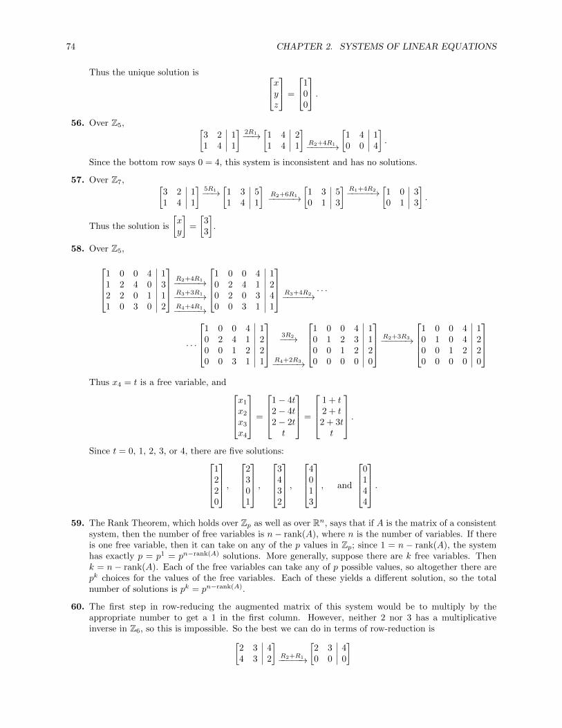
74 CHAPTER 2. SYSTEMS OF LINEAR EQUATIONS
Thus the unique solution is xyz
=
100
.56. Over Z5, [
3 2 11 4 1
]2R1−−→
[1 4 21 4 1
]R2+4R1−−−−−→
[1 4 10 0 4
].
Since the bottom row says 0 = 4, this system is inconsistent and has no solutions.
57. Over Z7, [3 2 11 4 1
]5R1−−→
[1 3 51 4 1
]R2+6R1−−−−−→
[1 3 50 1 3
]R1+4R2−−−−−→
[1 0 30 1 3
].
Thus the solution is
[xy
]=
[33
].
58. Over Z5,
1 0 0 4 11 2 4 0 32 2 0 1 11 0 3 0 2
R2+4R1−−−−−→R3+3R1−−−−−→R4+4R1−−−−−→
1 0 0 4 10 2 4 1 20 2 0 3 40 0 3 1 1
R3+4R2−−−−−→· · ·
· · ·
1 0 0 4 10 2 4 1 20 0 1 2 20 0 3 1 1
3R2−−→
R4+2R3−−−−−→
1 0 0 4 10 1 2 3 10 0 1 2 20 0 0 0 0
R2+3R3−−−−−→
1 0 0 4 10 1 0 4 20 0 1 2 20 0 0 0 0
Thus x4 = t is a free variable, and
x1
x2
x3
x4
=
1− 4t2− 4t2− 2tt
=
1 + t2 + t2 + 3tt
.Since t = 0, 1, 2, 3, or 4, there are five solutions:
1220
,
2301
,
3432
,
4013
, and
0144
.59. The Rank Theorem, which holds over Zp as well as over Rn, says that if A is the matrix of a consistent
system, then the number of free variables is n− rank(A), where n is the number of variables. If thereis one free variable, then it can take on any of the p values in Zp; since 1 = n − rank(A), the systemhas exactly p = p1 = pn−rank(A) solutions. More generally, suppose there are k free variables. Thenk = n − rank(A). Each of the free variables can take any of p possible values, so altogether there arepk choices for the values of the free variables. Each of these yields a different solution, so the totalnumber of solutions is pk = pn−rank(A).
60. The first step in row-reducing the augmented matrix of this system would be to multiply by theappropriate number to get a 1 in the first column. However, neither 2 nor 3 has a multiplicativeinverse in Z6, so this is impossible. So the best we can do in terms of row-reduction is[
2 3 44 3 2
]R2+R1−−−−−→
[2 3 40 0 0
]

Exploration: Lies My Computer Told Me 75
Thus y is a free variable, and 2x+ 3y = 4. To solve this equation, choose each possible value for y inturn:
• When y = 0, y = 2, or y = 4 we get 2x = 4, so that x = 2 or x = 5.
• When y = 1 or y = 3, we get 2x+ 3 = 4, or 2x = 1, which has no solution.
So altogether there are six solutions:[20
],
[50
],
[22
],
[52
],
[24
],
[54
].
Exploration: Lies My Computer Told Me
1.x+ y = 0x+ 801
800y = 0⇒ −800x− 800y = 0
800x+ 801y = 800⇒ x=−800
y = 800 .
2.x+ y = 0x+ 1.0012y = 0
⇒ −x− y = 0x+ 1.0012y = 1
⇒ x=−833.33y = 833.33 .
3. At four significant digits, we get
x+ y = 0x+ 1.001y = 0
⇒ −x− y = 0x+ 1.001y = 1
⇒ x=−1000y = 1000 ,
while at three significant digits, we get
x+ y = 0x+ 1.00y = 0
⇒ −x− y = 0x+ 1.00y = 1
⇒ Inconsistent system; no solution.
4. For the equations we just looked at, the slopes of the two lines were very close (the angle between thelines was very small). That means that changing one of the slopes even a little bit will result in alarge change in their intersection point. That is the cause of the wild changes in the computed outputvalues above — rounding to five significant digits is indeed the same as a small change in the slope ofthe second line, and it caused a large change in the computed solution.
For the second example, note that the two slopes are
7.083
4.552≈ 1.55602,
2.693
1.731≈ 1.55575,
so that again the slopes are close, so we would expect the same kind of behavior.
Exploration: Partial Pivoting
1. (a) Solving 0.00021x = 1 to five significant digits gives x = 10.00021 ≈ 4761.9.
(b) If only four significant digits are kept, we have 0.0002x = 1, so that x = 10.0002 = 5000. Thus the
effect of an error of 0.00001 in the input is an error of 238.1 in the result.
2. (a) Start by pivoting on 0.4. Multiply the first row by 10.4 = 250 to get [1, 249, 250]. Now we want
to subtract 75.3 times that row from the second row. Multiplying by 75.3 and keeping threesignificant digits gives
75.3[1, 249, 250] = [75.3, 18749.7, 18825.0] ≈ [75.3, 18700, 18800].
Then the second row becomes (again keeping only three significant digits)
[75.3, 45.3, 30]− [75.3, 18700, 18800] = [0, 18654.7, 18770] ≈ [0, 18700, 18800].

76 CHAPTER 2. SYSTEMS OF LINEAR EQUATIONS
This gives y = 1880018700 ≈ 1.00535 ≈ 1.01. Substituting back into the modified first row, which says
x+ 249y = 250 gives x = 250− 251.49 ≈ 250− 251 = −1.
Substituting x = y = 1 into the original system, however, yields two true equations, so this is infact the solution. The problem was that the large numbers in the second row, combined with thefact that we were keeping only three significant digits, overwhelmed the information from addingin the first row, so all that information was lost.
(b) First interchanging the rows gives the matrix[75.3 −45.3 300.4 99.6 100
]Multiply the first row by 1
75.3 to get (after reducing to three significant digits) [1,−0.602, 0.398].Then subtract 0.4 times that row from the second row:
[0.4, 99.6, 100]− 0.4[1,−0.602, 0.398] ≈ [0, 99.8, 99.8].
This gives 99.8y = 99.8, so that y = 1; from the first equation, we have x − 0.602y = 0.398, sothat x− 0.602 · 1 = 0.398 and thus x = 1. We get the correct answer.
3. (a) Without partial pivoting, we pivot on 0.001 to three significant digits, so we divide the first rowby 0.001, giving [1, 995, 1000], then multiply it by 10.2 and add the result to row 2, giving thematrix [
1 995 10000 −10100 −10200
]⇒ y ≈ 1.01.
Back-substituting gives x = 1.00−1.002 = 0 (again remembering to keep only three significant
digits). This error was introduced because 1.00 and −50.0 were ignored when reducing to threesignificant digits in the original row-reduction, being overwhelmed by numbers in the range of10000.
Using partial pivoting, we pivot on −10.2 to three significant digits: the second row becomes[1, 0.098, 4.9]. Then multiply it by 0.001 and subtract it from the first row, giving [0, 0.995, 1.00].Thus 0.995y = 1.00, so that to three significant digits y = 1.00. Back-substituting gives x =−50.0−1.00−10.2 = 51.0
10.2 = 5. Pivoting on the largest absolute value reduced the error in the solution.
(b) Start by pivoting on the 10.0 at upper left:10.0 −7.00 0.00 7.00−3.0 2.09 6.00 3.915.0 1.00 5.00 6.00
−→10.0 −7.00 0.00 7.00
0.0 −0.01 6.00 6.010.0 2.50 5.00 2.50
.If we continue, pivoting on −0.01 to three significant digits, the second row then becomes[0, 1,−600,−601]. Multiply it by 2.5 and add it to the third row:10.0 −7.00 0.00 7.00
0.0 −0.01 6.00 6.010.0 2.50 5.00 2.50
−→10.0 −7.00 0.00 7.00
0.0 −0.01 6.00 6.010.0 0 −1500 −1500
.This gives z = 1.00, y = −1.00, and x = 0.00.
If instead we reversed the second and third rows and pivoted on the 2.5, we would first dividethat row by 2.5, giving [0, 1, 2, 1], then multiply it by 0.01 and add it to the third row:10.0 −7.00 0.00 7.00
0.0 2.50 5.00 2.500.0 −0.01 6.00 6.01
−→10.0 −7.00 0.00 7.00
0.0 1 2 10.0 −0.01 6.00 6.01
−→10.0 −7.00 0.00 7.00
0.0 1 2 10.0 0 6.02 6.02
.This also gives z = 1.00, y = −1.00, and x = 0.00.

Exploration: An Introduction to the Analysis of Algorithms 77
Exploration: An Introduction to the Analysis of Algorithms
1. We count the number of operations, one step at a time. 2 4 6 83 9 6 12−1 1 −1 1
12R1−−−→
1 2 3 43 9 6 12−1 1 −1 1
There were three operations here: 1
2 · 4 = 2, 12 · 6 = 3, and 1
2 · 8 = 4. We don’t count 12 · 2 = 1 since we
don’t actually perform that operation — once we chose 2, we knew we were going to turn it into 1. 1 2 3 43 9 6 12−1 1 −1 1
R2−3R1−−−−−→
1 2 3 40 3 −3 0−1 1 −1 1
There were three operations here: 3 · 2 = 6, 3 · 3 = 9, and 3 · 4 = 12, fr a total of six operations so far.Note that we are counting only multiplications and divisions, and that again we don’t count 3 · 1 = 3since we didn’t actually have to perform it — we just replace the 3 in the second row by a 0. 1 2 3 4
0 3 −3 0−1 1 −1 1
R3+R1−−−−−→
1 2 3 40 3 −3 00 3 2 5
There were 3 operations here: 1 · 2 = 2, 1 · 3 = 3, and 1 · 4 = 4, for a total of nine operations so far.1 2 3 4
0 3 −3 00 3 2 5
13R2−−−→
1 2 3 40 1 −1 00 3 2 5
In this step, there were 2 operations: 1
3 · (−3) and 13 · 0 = 0, for a total of eleven so far.1 2 3 4
0 1 −1 00 3 2 5
R3−3R2−−−−−→
1 2 3 40 1 −1 00 0 5 5
In this step, there were 2 operations: −3 · (−1) = 3 and −3 · 0 = 0, for a total of 13 so far.1 2 3 4
0 1 −1 00 0 5 5
15R3−−−→
1 2 3 40 1 −1 00 0 1 1
In this step, there was one operation, 1
5 · 5 = 1, for a total of 14.
Finally, to complete the back-substitution, we need three more operations: −1 ·x3 to find x2, and 2 ·x2
and 3 · x3 to find x1. So in total 17 operations were required.
2. To compute the reduced row echelon form, we first compute the row echelon form above, which took14 operations. Then: 1 2 3 4
0 1 −1 00 0 1 1
R1−2R2−−−−−→1 0 5 4
0 1 −1 00 0 1 1
This required two operations, −2 · (−1) and −2 · 0, for a total of 16. Finally,1 0 5 4
0 1 −1 00 0 1 1
R1−5R3−−−−−→R2+R3−−−−−→
1 0 0 −10 1 0 10 0 1 1

78 CHAPTER 2. SYSTEMS OF LINEAR EQUATIONS
This required two operations, both in the constant column: 1 ·1 and −5 ·1, for a total of 18. So for thisexample, Gauss-Jordan required one more operation than Gaussian elimination. We would probablyneed more data to conclude that it is generally less efficient.
3. (a) There are n operations required to create the first leading 1 because we have to divide every entryin the first row, except a11, by a11 (we don’t have to divide a11 by itself because the 1 resultsfrom the choice of pivot. Next, there are n operations required to create the first zero in column1, because we have to multiply every entry in the first row, except the 1 in column one, by a21.Again, we don’t have to multiply the 1 by itself, since we know we are simply replacing a21 byzero. Similarly, there are n operations required to create each zero in column 1. Since there aren − 1 rows excluding the first row, introducing the 1 in row one and the zeros below it requiresn+ (n− 1)n = n2 operations.
(b) We can think of the resulting matrix, below and to the right of a22, as an (n− 1)× n augmentedmatrix. Applying the process in part (a) to this matrix, we see that turning a22 into a 1 andcreating zeros below it requires (n− 1) + (n− 2)(n− 1) = (n− 1)2 operations. Continuing to thematrix starting at row 3, column 3; this requires (n− 2)2 operations. So altogether, to reduce thematrix to row echelon form requires n2 + (n− 1)2 + · · ·+ 22 + 12 operations.
(c) To find xn−1 requires one operation: we must multiply xn by the entry an−1,n. Then there aretwo operations required to find xn−2, and so forth, until we require n − 1 operations to find x1.So the total number required for the back-substitution is 1 + 2 + · · ·+ (n− 1).
(d) From Appendix B, we see that
12 + 22 + · · ·+ k2 =k(k + 1)(2k + 1)
6
1 + 2 + · · ·+ k =k(k + 1)
2.
Thus the total number of operations required is
12 + 22 + · · ·+ n2 + 1 + 2 + · · ·+ (n− 1) =n(n+ 1)(2n+ 1)
6+n(n− 1)
2
=1
3n3 +
1
2n2 +
1
6n+
1
2n2 − 1
2n
=1
3n3 + n2 − 1
3n.
For large values of n, the cubic term dominates, so the total number of operations required is≈ 1
3n3.
4. As we saw in Exercise 2 in this section, we get the same n2 + (n− 1)2 + · · ·+ 22 + 12 operations to getthe matrix into row echelon form. Then to create the 1 zero above row 2 requires 1(n− 1) operations,since each of the remaining n− 1 entries in row 2 must be multiplied. To create the 2 zeros above row3 requires 2(n − 2) operations, since each of the remaining entries in row 3 must be multiplied twice.Continuing, we see that the total number of operations is
(n− 1) + 2(n− 2) + · · ·+(n− 1)(n− (n− 1))
= (1 · n+ 2 · n+ · · ·+ (n− 1) · n)− (12 + 22 + · · ·+ (n− 1)2)
= n(1 + 2 + · · ·+ (n− 1))− (12 + 22 + · · ·+ (n− 1)2).
Adding that to the operations required to get the matrix into row echelon form, and using the formulas

2.3. SPANNING SETS AND LINEAR INDEPENDENCE 79
from Appendix B, we get for the total number of operations
n2 + (n− 1)2 + · · ·+ 22 + 12 + n(1 + 2 + · · ·+ (n− 1))−(12 + 22 + · · ·+ (n− 1))2
= n2 + n · n(n− 1)
2
= n2 +1
2n3 − 1
2n2
=1
2n3 +
1
2n2.
Again, for large values of n, the cubic term dominates, so the total number of operations required is≈ 1
2n3.
2.3 Spanning Sets and Linear Independence
1. Yes, it is. We want to write
x
[1−1
]+ y
[2−1
]=
[12
],
so we want to solve the system of linear equations
x+ 2y = 1
−x− y = 2.
Row reducing the augmented matrix for the system gives[1 2 1−1 −1 2
]R2+R1−−−−−→
[1 2 10 1 3
]R1−2R2−−−−−→
[1 0 −50 1 3
].
So the solution is x = −5 and y = 3, and the linear combination is v = −5u1 + 3u2.
2. No, it is not. We want to write
x
[4−2
]+ y
[−2
1
]=
[21
],
so we want to solve the system of linear equations
4x− 2y = 2
−2x+ y = 1
Row-reducing the augmented matrix for the system gives[4 −2 2
−2 1 1
] 14R1−−−→
[1 − 1
212
−2 1 1
]R2+2R1−−−−−→
[1 − 1
212
0 0 2
]So the system is inconsistent, and the answer follows from Theorem 2.4.
3. No, it is not. We want to write
x
110
+ y
011
=
123
,so we want to solve the system of linear equations
x = 1
x+ y = 2
y = 3.
Rather than constructing the matrix and reducing it, note that the first and third equations force x = 1and y = 3, and that these values of x and y do not satisfy the second equation. Thus the system isinconsistent, so that v is not a linear combination of u1 and u2.

80 CHAPTER 2. SYSTEMS OF LINEAR EQUATIONS
4. Yes, it is. We want to write
x
110
+ y
011
=
32−1
,so we want to solve the system of linear equations
x = 3
x+ y = 2
y = −1
Rather than constructing the matrix and reducing it, note that the first and third equations force x = 3and y = −1, and that these values of x and y also satisfy the second equation. Thus v = 3u1 − u2.
5. Yes, it is. We want to write
x
110
+ y
011
+ z
101
=
123
,so we want to solve the system of linear equations
x +z = 1
x+ y = 2
y+z = 3.
Row-reducing the associated augmented matrix gives1 0 1 11 1 0 20 1 1 3
R2−R1−−−−−→
1 0 1 10 1 −1 10 1 1 3
R3−R2−−−−−→
1 0 1 10 1 −1 10 0 2 2
12R3−−−→
· · ·
· · ·
1 0 1 10 1 −1 10 0 1 1
R1−R3−−−−−→R2+R3−−−−−→
1 0 0 00 1 0 20 0 1 1
This gives the solution x = 0, y = 2, and z = 1, so that v = 2u2 + u3.
6. Yes, it is. The associated linear system is
1.0x+ 3.4y − 1.2z = 3.2
0.4x+ 1.4y + 0.2z = 2.0
4.8x− 6.4y − 1.0z = −2.6
Solving this system with a CAS gives x = 1.0, y = 1.0, z = 1.0, so that v = u1 + u2 + u3.
7. Yes, it is. b is in the span of the columns of A if and only if the system Ax = b has a solution, whichis to say if and only if the linear system
x+ 2y = 5
3x+ 4y = 6
has a solution. Row-reducing the augmented matrix for the system gives[1 2 5
3 4 6
]R2−3R1−−−−−→
[1 2 5
0 −2 −9
]− 1
2R2−−−−→
[1 2 5
0 1 92
]R1−2R2−−−−−→
[1 0 −4
0 1 92
]
Thus x = −4 and y = 92 , so that
A
[−4
92
]=
[56
].
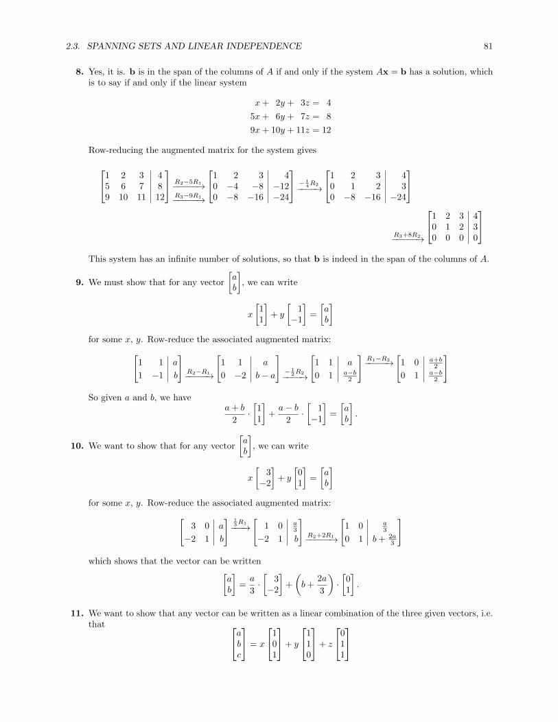
2.3. SPANNING SETS AND LINEAR INDEPENDENCE 81
8. Yes, it is. b is in the span of the columns of A if and only if the system Ax = b has a solution, whichis to say if and only if the linear system
x+ 2y + 3z = 4
5x+ 6y + 7z = 8
9x+ 10y + 11z = 12
Row-reducing the augmented matrix for the system gives
1 2 3 45 6 7 89 10 11 12
R2−5R1−−−−−→R3−9R1−−−−−→
1 2 3 40 −4 −8 −120 −8 −16 −24
− 14R2−−−−→
1 2 3 40 1 2 30 −8 −16 −24
R3+8R2−−−−−→
1 2 3 40 1 2 30 0 0 0
This system has an infinite number of solutions, so that b is indeed in the span of the columns of A.
9. We must show that for any vector
[ab
], we can write
x
[11
]+ y
[1−1
]=
[ab
]for some x, y. Row-reduce the associated augmented matrix:[
1 1 a
1 −1 b
]R2−R1−−−−−→
[1 1 a
0 −2 b− a
]− 1
2R2−−−−→
[1 1 a
0 1 a−b2
]R1−R2−−−−−→
[1 0 a+b
2
0 1 a−b2
]
So given a and b, we havea+ b
2·[11
]+a− b
2·[
1−1
]=
[ab
].
10. We want to show that for any vector
[ab
], we can write
x
[3−2
]+ y
[01
]=
[ab
]for some x, y. Row-reduce the associated augmented matrix:[
3 0 a
−2 1 b
] 13R1−−−→
[1 0 a
3
−2 1 b
]R2+2R1−−−−−→
[1 0 a
3
0 1 b+ 2a3
]
which shows that the vector can be written[ab
]=a
3·[
3−2
]+
(b+
2a
3
)·[01
].
11. We want to show that any vector can be written as a linear combination of the three given vectors, i.e.that ab
c
= x
101
+ y
110
+ z
011

82 CHAPTER 2. SYSTEMS OF LINEAR EQUATIONS
for some x, y, z. Row-reduce the associated augmented matrix:1 1 0 a0 1 1 b1 0 1 c
R3−R1−−−−−→
1 1 0 a0 1 1 b0 −1 1 c− a
R3+R2−−−−−→
1 1 0 a0 1 1 b0 0 2 b+ c− a
12R3−−−→
1 1 0 a
0 1 1 b
0 0 1 b+c−a2
R2−R3−−−−−→
1 1 0 a
0 1 0 a+b−c2
0 0 1 b+c−a2
R1−R2−−−−−→
1 0 0 a−b+c2
0 1 0 a+b−c2
0 0 1 b+c−a2
Thus ab
c
=1
2(a− b+ c) ·
101
+1
2(a+ b− c) ·
110
+1
2(−a+ b+ c) ·
011
.12. We want to show that any vector can be written as a linear combination of the three given vectors, i.e.
that abc
= x
110
+ y
123
+ z
21−1
for some x, y, z. Row-reduce the associated augmented matrix:
1 1 2 a1 2 1 b0 3 −1 c
R2−R1−−−−−→
1 1 2 a0 1 −1 b− a0 3 −1 c
R3−3R2−−−−−→
1 1 2 a0 1 −1 b− a0 0 2 c+ 3a− 3b
12R3−−−→
1 1 2 a
0 1 −1 b− a0 0 1 1
2 (c+ 3a− 3b)
R1−2R3−−−−−→R2+R3−−−−−→
1 1 0 3b− 2a− c0 1 0 1
2 (c+ a− b)0 0 1 1
2 (c+ 3a− 3b)
R1−R2−−−−−→
1 0 0 12 (7b− 5a− 3c)
0 1 0 12 (c+ a− b)
0 0 1 12 (c+ 3a− 3b)
Thus ab
c
=1
2(7b− 5a− 3c)
110
+1
2(c+ a− b)
123
+1
2(c+ 3a− 3b)
21−1
.13. (a) Since
[2−4
]= −2
[−1
2
], these vectors are parallel, so their span is the line through the origin with
direction vector
[−1
2
].
(b) The vector equation of this line is
[xy
]= t
[−1
2
]. Note that this is just another way of saying
that the line is the span of the given vector. To derive the general equation of the line, expandthe above, giving the parametric equations x = −t and y = 2t. Substitute −x for t in the secondequation, giving y = −2x, or 2x+ y = 0.

2.3. SPANNING SETS AND LINEAR INDEPENDENCE 83
14. (a) Since the span of
[00
]is just the origin, and the origin is in the span of
[34
], the span of these two
vectors is just the span of
[34
], which is the line through the origin with direction vector
[34
].
(b) The vector equation of this line is
[xy
]= t
[34
]. Note that this is just another way of saying that
the line is the span of the given vector. To derive the general equation of the line, expand theabove, giving the parametric equations x = 3t and y = 4t. Substitute 1
3x for t in the secondequation, giving y = 4
3x. Clearing fractions gives 3y = 4x, or 4x− 3y = 0.
15. (a) Since the given vectors are not parallel, their span is a plane through the origin containing thesetwo vectors as direction vectors.
(b) The vector equation of the plane is xyz
= s
120
+ t
32−1
.One way of deriving the general equation of the plane is to solve the system of equations arisingfrom the above vector equation. Row-reducing the corresponding augmented system gives1 3 x
2 2 y0 −1 z
R2−2R2−−−−−→
1 3 x0 −4 y − 2x0 −1 z
R3− 1
4R2−−−−−−→
1 3 x0 −4 y − 4x0 0 z + 1
4 (2x− y)
Since we know the system is consistent, the bottom row must consist entirely of zeros. Thusthe points on the plane must satisfy z + 1
4 (2x − y) = 0, or 4z + 2x − y = 0. This is the plane2x− y + 4z = 0.
An alternative method is to find a normal vector to the plane by taking the cross-product of thetwo given vectors: 1
20
× 3
2−1
=
0 · 2− 2 · (−1)1 · (−1)− 0 · 3
2 · 3− 1 · 2
=
2−1
4
.So the equation of the plane is 2x − y + 4z = d; since it passes through the origin, we again get2x− y + 4z = 0.
16. (a) First, note that 0−1
1
= −
10−1
−−1
10
,so that the third vector is in the span of the first two. So we need only consider the first two
vectors. Their span is the plane through the origin with direction vectors
10−1
and
−110
.
(b) The vector equation of this plane is
s
10−1
+ t
−110
=
xyz
.To find the general equation of the plane, we can solve the corresponding system of equations fors and t. Row-reducing the augmented matrix gives 1 −1 x
0 1 y
−1 0 z
R3+R1−−−−−→
1 −1 x
0 1 y
0 −1 x+ z
R3+R2−−−−−→
1 −1 x
0 1 y
0 0 x+ y + z

84 CHAPTER 2. SYSTEMS OF LINEAR EQUATIONS
Since we know the system is consistent, the bottom row must consist of all zeros, so that pointson the plane satisfy the equation x+ y + z = 0.
Alternatively, we could find a normal vector to the plane by taking the cross product of thedirection vectors: 1
0−1
×−1
10
=
0 · 0− (−1) · 1−1 · −1− 1 · 01 · 1− 0 · (−1)
=
111
.Thus the equation of the plane is x+ y + z = d; since it passes through the origin, we again getx+ y + z = 0.
17. Substituting the two points (1, 0, 3) and (−1, 1,−3) into the equation for the plane gives a linear systemin a, b, and c:
a + 3c = 0
−a+ b− 3c = 0.
Row-reducing the associated augmented matrix gives[1 0 3 0−1 1 −3 0
]R2+R1−−−−−→
[1 0 3 00 1 0 0
],
so that b = 0 and a = −3c. Thus the equation of the plane is −3cx + cz = 0. Clearly we must havec 6= 0, since otherwise we do not get a plane. So dividing through by c gives −3x+z = 0, or 3x−z = 0,for the general equation of the plane.
18. Note that
u = 1u + 0v + 0w, v = 0u + 1v + 0w, w = 0u + 0v + 1w.
Or, if one adopts the usual convention of not writing terms with coefficients of zero, u is in the spanbecause u = u.
19. Note that
u = u,
v = (u + v)− u,
w = (u + v + w)− (u + v),
and the terms in parentheses on the right, together with u, are the elements of the given set.
20. (a) To prove the statement, we must show that anything that can be written as a linear combinationof the elements of S can also be written as a linear combination of the elements of T . But if x isa linear combination of elements of S, then
x = a1u1 + a2u2 + · · ·+ akuk
= a1u1 + a2u2 + · · ·+ akuk + 0uk+1 + 0uk+1 + · · ·+ 0um.
This shows that x is also a linear combination of elements of T , proving the result.
(b) We know that span(S) ⊆ span(T ) from part (a). Since T is a set of vectors in Rn, we know thatspan(T ) ⊆ Rn. But then
Rn = span(S) ⊆ span(T ) ⊆ Rn,
so that span(T ) = Rn.

2.3. SPANNING SETS AND LINEAR INDEPENDENCE 85
21. (a) Suppose that
ui = ui1v1 + ui2v2 + · · ·+ uimvm, i = 1, 2, . . . , k.
Suppose that w is a linear combination of the ui. Then
w = w1u1 + w2u2 + · · ·+ wkuk
= w1(u11v1 + u12v2 + · · ·+ u1mvm) + w2(u21v1 + u22v2 + · · ·+ u2mvm) + · · ·wk(uk1v1 + uk2v2 + · · ·+ ukmvm)
= (w1u11 + w2u21 + · · ·+ wkuk1)v1 + (w1u12 + w2u22 + · · ·+ wkuk2)v2 + · · ·(w1u1m + w2u2m + · · ·+ wkukm)vm
= w′1v1 + w′2v2 + · · ·+ w′mvm.
This shows that w is a linear combination of the vj . Thus span(u1, . . . ,uk) ⊆ span(v1, . . . ,vk).
(b) Reversing the roles of the u’s and the v’s in part (a) gives span(v1, . . . ,vk) ⊆ span(u1, . . . ,uk).Combining that with part (a) shows that each of the spans is contained in the other, so they areequal.
(c) Let
u1 =
100
, u2 =
110
, u3 =
111
.We want to show that each ui is a linear combination of e1, e2, and e3, and the reverse. Thefirst of these is obvious: since e1, e2, and e3 span R3, any vector is R3 is a linear combination ofthose, so in particular u1, u2, and u3 are. Next, note that
e1 = u1
e2 = u2 − u1
e3 = u3 − u2,
so that the ej are linear combinations of the ui. Part (b) then implies that span(u1,u2,u3) =span(e1, e2, e3) = R3.
22. The vectors
2−1
3
and
−123
are not scalar multiples of one another, so are linearly independent.
23. There is no obvious dependence relation, so follow Example 2.23. We want scalars c1, c2, c3 so that
c1
111
+ c2
123
+ c3
1−1
2
=
000
.Row-reduce the associated augmented matrix:
1 1 1 01 2 −1 01 3 2 0
R2−R1−−−−−→R3−R1−−−−−→
1 1 1 00 1 −2 00 2 1 0
R3−2R2−−−−−→
1 1 1 00 1 −2 00 0 5 0
15R3−−−→
· · ·
· · ·
1 1 1 00 1 −2 00 0 1 0
R1−R3−−−−−→R2+2R3−−−−−→
1 1 0 00 1 0 00 0 1 0
R1−R3−−−−−→1 0 0 0
0 1 0 00 0 1 0
Thus the system has only the solution c1 = c2 = c3 = 0, so the vectors are linearly independent.
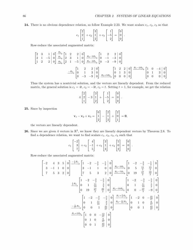
86 CHAPTER 2. SYSTEMS OF LINEAR EQUATIONS
24. There is no obvious dependence relation, so follow Example 2.23. We want scalars c1, c2, c3 so that
c1
221
+ c2
312
+ c3
1−5
2
=
000
.Row-reduce the associated augmented matrix:
2 3 1 02 1 −5 01 2 2 0
R3−−→R1−−→R2−−→
1 2 2 02 3 1 02 1 −5 0
R2−2R1−−−−−→R3−2R1−−−−−→
1 2 2 00 −1 −3 00 −3 −9 0
−R2−−−→
1 2 2 00 1 3 00 −3 −9 0
R3+3R2−−−−−→
1 2 2 00 1 3 00 0 0 0
R1−2R2−−−−−→1 0 −4 0
0 1 3 00 0 0 0
Thus the system has a nontrivial solution, and the vectors are linearly dependent. From the reducedmatrix, the general solution is c1 = 4t, c2 = −3t, c3 = t. Setting t = 1, for example, we get the relation
4
221
− 3
312
+
1−5
2
=
000
.25. Since by inspection
v1 − v2 + v3 =
012
−2
13
+
201
= 0,
the vectors are linearly dependent.
26. Since we are given 4 vectors in R3, we know they are linearly dependent vectors by Theorem 2.8. Tofind a dependence relation, we want to find scalars c1, c2, c3, c4 such that
c1
−237
+ c2
4−1
5
+ c3
313
+ c4
502
=
000
.Row-reduce the associated augmented matrix:
−2 4 3 5 0
3 −1 1 0 0
7 5 3 2 0
− 1
2R1−−−−→
1 −2 − 32 − 5
2 0
3 −1 1 0 0
7 5 3 2 0
R2−3R1−−−−−→R3−7R1−−−−−→
1 −2 − 3
2 − 52 0
0 5 112
152 0
0 19 272
392 0
15R2−−−→
1 −2 − 3
2 − 52 0
0 1 1110
32 0
0 19 272
392 0
R3−19R2−−−−−−→
1 −2 − 3
2 − 52 0
0 1 1110
32 0
0 0 − 375 −9 0
− 537R3−−−−→
1 −2 − 3
2 − 52 0
0 1 1110
32 0
0 0 1 4537 0
R1+ 3
2R3−−−−−−→R2− 11
10R3−−−−−−→
1 −2 0 − 25
37 0
0 1 0 637 0
0 0 1 4537 0
R1+2R2−−−−−→
1 0 0 − 13
37 0
0 1 0 637 0
0 0 1 4537 0
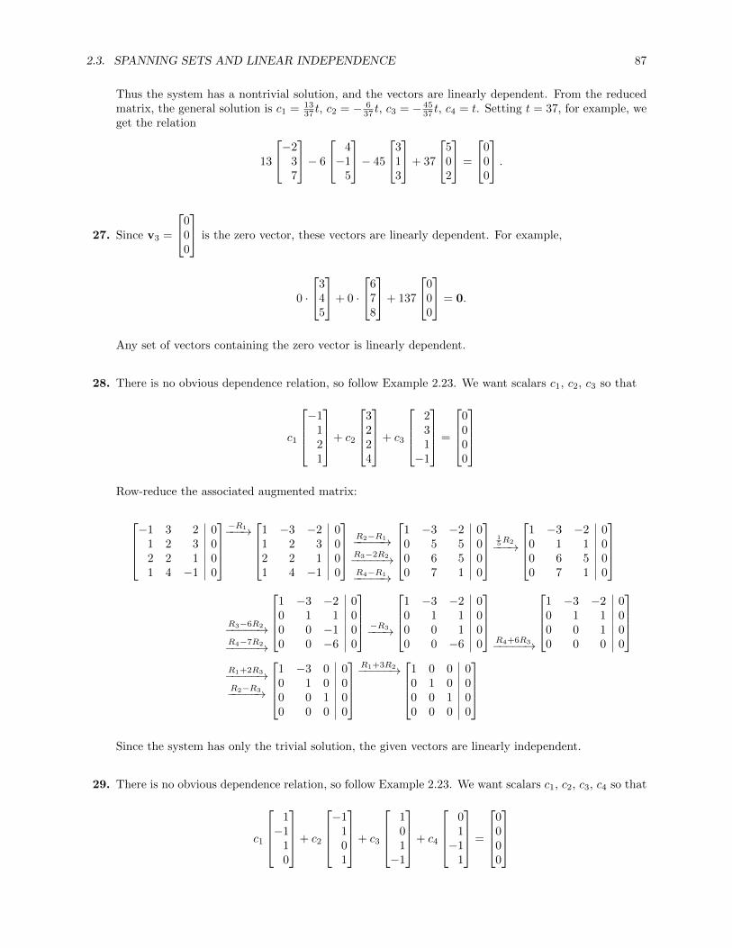
2.3. SPANNING SETS AND LINEAR INDEPENDENCE 87
Thus the system has a nontrivial solution, and the vectors are linearly dependent. From the reducedmatrix, the general solution is c1 = 13
37 t, c2 = − 637 t, c3 = − 45
37 t, c4 = t. Setting t = 37, for example, weget the relation
13
−237
− 6
4−1
5
− 45
313
+ 37
502
=
000
.
27. Since v3 =
000
is the zero vector, these vectors are linearly dependent. For example,
0 ·
345
+ 0 ·
678
+ 137
000
= 0.
Any set of vectors containing the zero vector is linearly dependent.
28. There is no obvious dependence relation, so follow Example 2.23. We want scalars c1, c2, c3 so that
c1
−1
121
+ c2
3224
+ c3
231−1
=
0000
Row-reduce the associated augmented matrix:
−1 3 2 0
1 2 3 02 2 1 01 4 −1 0
−R1−−−→
1 −3 −2 01 2 3 02 2 1 01 4 −1 0
R2−R1−−−−−→R3−2R2−−−−−→R4−R1−−−−−→
1 −3 −2 00 5 5 00 6 5 00 7 1 0
15R2−−−→
1 −3 −2 00 1 1 00 6 5 00 7 1 0
R3−6R2−−−−−→R4−7R2−−−−−→
1 −3 −2 00 1 1 00 0 −1 00 0 −6 0
−R3−−−→
1 −3 −2 00 1 1 00 0 1 00 0 −6 0
R4+6R3−−−−−→
1 −3 −2 00 1 1 00 0 1 00 0 0 0
R1+2R3−−−−−→R2−R3−−−−−→
1 −3 0 00 1 0 00 0 1 00 0 0 0
R1+3R2−−−−−→
1 0 0 00 1 0 00 0 1 00 0 0 0
Since the system has only the trivial solution, the given vectors are linearly independent.
29. There is no obvious dependence relation, so follow Example 2.23. We want scalars c1, c2, c3, c4 so that
c1
1−1
10
+ c2
−1
101
+ c3
101−1
+ c4
01−1
1
=
0000

88 CHAPTER 2. SYSTEMS OF LINEAR EQUATIONS
Row-reduce the associated augmented matrix:1 −1 1 0 0−1 1 0 1 0
1 0 1 −1 00 1 −1 1 0
R2+R1−−−−−→R3−R1−−−−−→
1 −1 1 0 00 0 1 1 00 1 0 −1 00 1 −1 1 0
R2↔R3−−−−−→
1 −1 1 0 00 1 0 −1 00 0 1 1 00 1 −1 1 0
R4−R2−−−−−→
1 −1 1 0 00 1 0 −1 00 0 1 1 00 0 −1 2 0
R4+R3−−−−−→
1 −1 1 0 00 1 0 −1 00 0 1 1 00 0 0 3 0
13R4−−−→
1 −1 1 0 00 1 0 −1 00 0 1 1 00 0 0 1 0
R2+R4−−−−−→R3−R4−−−−−→
1 −1 1 0 00 1 0 0 00 0 1 0 00 0 0 1 0
R1+R2−R3−−−−−−−→
1 0 0 0 00 1 0 0 00 0 1 0 00 0 0 1 0
Since the system has only the trivial solution, the given vectors are linearly independent.
30. The vectors
v1 =
0001
, v2 =
0021
, v3 =
0321
, v4 =
4321
are linearly dependent. For suppose c1v1 + c2v2 + c3v3 + c4v4 = 0. Then c4 must be zero in order forthe first component of the sum to be zero. But then the only vector containing a nonzero entry in thesecond component is v3, so that c3 = 0 as well. Now for the same reason c2 = 0, looking at the thirdcomponent. Finally, that implies that c1 = 0. So the vectors are linearly independent.
31. By inspection
v1 + v2 − v3 + v4 =
3−1
1−1
+
−1
31−1
−
1131
+
−1−1
13
= 0,
so the vectors are linearly dependent.
32. Construct a matrix A with these vectors as its rows and try to produce a zero row:[2 −1 3−1 2 3
]R′1=R1+R2−−−−−−−→
[1 1 6−1 2 3
]R′2=R2+2R′1−−−−−−−−→
[1 1 60 3 9
]This matrix is in row echelon form and has no zero rows, so the matrix has rank 2 and the vectors arelinearly independent by Theorem 2.7.
33. Construct a matrix A with these vectors as its rows and try to produce a zero row:1 1 11 2 31 −1 2
R′2=R2−R1−−−−−−−→R′3=R3−R1−−−−−−−→
1 1 10 1 20 −2 1
R′′3 =R′3+2R′2−−−−−−−−→
1 1 10 1 20 0 5
This matrix is in row echelon form and has no zero rows, so the matrix has rank 3 and the vectors arelinearly independent by Theorem 2.7.

2.3. SPANNING SETS AND LINEAR INDEPENDENCE 89
34. Construct a matrix A with these vectors as its rows and try to produce a zero row:2 2 13 1 21 −5 2
R1↔R3−−−−−→
1 −5 23 1 22 2 1
R′2=R2−3R1−−−−−−−−→R′3=R3−2R1−−−−−−−−→
1 −5 20 16 −40 12 −3
R′′3 =R′3− 3
4R′2−−−−−−−−−→
1 −5 20 12 −30 0 0
Since there is a zero row, the matrix has rank less than 3, so the vectors are linearly dependent byTheorem 2.7. Working backwards, we have
[0, 0, 0] = R′′3 = R′3 −3
4R′2 = R3 − 2R1 −
3
4(R2 − 3R1) =
1
4R1 −
3
4R2 +R3
=1
4
1−5
2
− 3
4
312
+
221
.35. Construct a matrix A with these vectors as its rows and try to produce a zero row:0 1 2
2 1 32 0 1
R′1=R2−−−−−→R′2=R1−−−−−→
2 1 30 1 22 0 1
R′3=R3−R′1−−−−−−−→
2 1 30 1 20 −1 −2
R′′3 =R′3+R′2−−−−−−−−→
2 1 30 1 10 0 0
This matrix is in row echelon form and has a zero row, so the vectors are linearly dependent by Theorem2.7. Working backwards, we have
[0, 0, 0] = R′′3 = R′3 +R′2 = R3 −R′1 +R′2 = R3 −R2 +R1 = R1 −R2 +R3 =
012
−2
13
+
201
.36. Construct a matrix A with these vectors and try to produce a zero row:
−2 3 7
4 −1 5
3 1 3
5 0 2
R′2=R2+2R1−−−−−−−−→R′3=R3+ 3
2R1−−−−−−−−→R′4=R4+ 5
2R1−−−−−−−−→
−2 3 7
0 5 19
0 112
272
0 152
392
R′′3 =2R′3−−−−−→R′′4 =2R′4−−−−−→
−2 3 7
0 5 19
0 11 27
0 15 39
· · ·
· · · R′′′3 =R′′3− 115 R′2−−−−−−−−−−→
R′′′4 =R′′4−3R′2−−−−−−−−−→
−2 3 7
0 5 19
0 0 − 745
0 0 −18
R′′′′4 =R′′′4 − 5·18
74 R′′′3−−−−−−−−−−−−→
−2 3 7
0 5 19
0 0 − 745
0 0 0
Since this matrix has a zero row, it has rank less than 2, so the vectors are linearly dependent. Workingbackwards, we have
[0, 0, 0] = R′′′′4 = R′′′4 −90
74R′′′3
= R′′4 − 3R′2 −45
37
(R′′3 −
11
5R′2
)= 2R′4 − 3R′2 −
90
37R′3 +
99
37R′2
= 2
(R4 +
5
2R1
)− 3(R2 + 2R1)− 90
37
(R3 +
3
2R1
)+
99
37(R2 + 2R1)
=26
37R1 −
12
37R2 −
90
37R3 + 2R4.
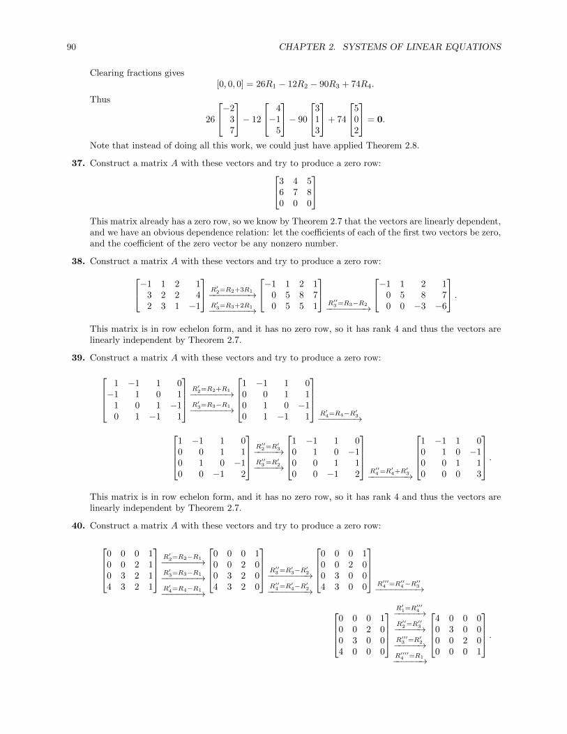
90 CHAPTER 2. SYSTEMS OF LINEAR EQUATIONS
Clearing fractions gives[0, 0, 0] = 26R1 − 12R2 − 90R3 + 74R4.
Thus
26
−237
− 12
4−1
5
− 90
313
+ 74
502
= 0.
Note that instead of doing all this work, we could just have applied Theorem 2.8.
37. Construct a matrix A with these vectors and try to produce a zero row:3 4 56 7 80 0 0
This matrix already has a zero row, so we know by Theorem 2.7 that the vectors are linearly dependent,and we have an obvious dependence relation: let the coefficients of each of the first two vectors be zero,and the coefficient of the zero vector be any nonzero number.
38. Construct a matrix A with these vectors and try to produce a zero row:−1 1 2 13 2 2 42 3 1 −1
R′2=R2+3R1−−−−−−−−→R′3=R3+2R1−−−−−−−−→
−1 1 2 10 5 8 70 5 5 1
R′′3 =R3−R2−−−−−−−−→
−1 1 2 10 5 8 70 0 −3 −6
.This matrix is in row echelon form, and it has no zero row, so it has rank 4 and thus the vectors arelinearly independent by Theorem 2.7.
39. Construct a matrix A with these vectors and try to produce a zero row:
1 −1 1 0−1 1 0 1
1 0 1 −10 1 −1 1
R′2=R2+R1−−−−−−−→R′3=R3−R1−−−−−−−→
1 −1 1 00 0 1 10 1 0 −10 1 −1 1
R′4=R4−R′3−−−−−−−→
1 −1 1 00 0 1 10 1 0 −10 0 −1 2
R′′2 =R′3−−−−−→R′′3 =R′2−−−−−→
1 −1 1 00 1 0 −10 0 1 10 0 −1 2
R′′4 =R′4+R′3−−−−−−−−→
1 −1 1 00 1 0 −10 0 1 10 0 0 3
.This matrix is in row echelon form, and it has no zero row, so it has rank 4 and thus the vectors arelinearly independent by Theorem 2.7.
40. Construct a matrix A with these vectors and try to produce a zero row:
0 0 0 10 0 2 10 3 2 14 3 2 1
R′2=R2−R1−−−−−−−→R′3=R3−R1−−−−−−−→R′4=R4−R1−−−−−−−→
0 0 0 10 0 2 00 3 2 04 3 2 0
R′′3 =R′3−R′2−−−−−−−−→
R′′4 =R′4−R′2−−−−−−−−→
0 0 0 10 0 2 00 3 0 04 3 0 0
R′′′4 =R′′4−R
′′3−−−−−−−−→
0 0 0 10 0 2 00 3 0 04 0 0 0
R′1=R′′′4−−−−−→R′′2 =R′′3−−−−−→R′′′3 =R′2−−−−−→R′′′′4 =R1−−−−−−→
4 0 0 00 3 0 00 0 2 00 0 0 1
.

2.3. SPANNING SETS AND LINEAR INDEPENDENCE 91
This matrix is in row echelon form, and it has no zero row, so it has rank 4 and thus the vectors arelinearly independent by Theorem 2.7.
41. Construct a matrix A with these vectors and try to produce a zero row:
3 −1 1 −1−1 3 1 −1
1 1 3 1−1 −1 1 3
R′1=R3−−−−−→
R′3=R1−−−−−→
1 1 3 1−1 3 1 −1
3 −1 1 −1−1 −1 1 3
R′2=R2+R′1−−−−−−−→R′′3 =R′3−3R′1−−−−−−−−→R′4=R4+R′1−−−−−−−→
1 1 3 10 4 4 00 −4 −8 −40 0 4 4
R′′′3 =R′′3 +R′2+R′4−−−−−−−−−−−→
1 1 3 10 4 4 00 0 0 00 0 4 4
.Since this matrix has a zero row, it has rank less than 4, so the vectors are linearly dependent. Workingbackwards, we have
[0, 0, 0, 0] = R′′′3 = R′′3 +R′2 +R′4
= R′3 − 3R′1 +R2 +R′1 +R4 +R′1
= R′3 −R′1 +R2 +R4
= R1 −R3 +R2 +R4.
Thus 3−1
1−1
+
−1
31−1
−
1131
+
−1−1
13
= 0.
42. (a) In this case, rank(A) = n. To see this, recall that v1, v2, . . . , vn are linearly independent if andonly if the only solution of [A | 0] = [v1 v2 . . . vn | 0] is the trivial solution. Since the trivialsolution is always a solution, it is the only one if and only if the number of free variables in theassociated system is zero. Then the Rank Theorem (Theorem 2.2 in Section 2.2) says that thenumber of free variables is n− rank(A), so that n = rank(A).
(b) Let
A =
v1
v2
...vn
.Then by Theorem 2.7, the vectors, which are the rows of A, are linearly independent if and onlyif the rank of A is greater than or equal to n. But A has n rows, so its rank is at most n. Thus,the rows of A are linearly independent if and only if the rank of A is exactly n.
43. (a) Yes, they are. Suppose that c1(u + v) + c2(v + w) + c3(u + w) = 0. Expanding gives
c1u + c1v + c2v + c2w + c3u + c3w = (c1 + c3)u + (c1 + c2)v + (c2 + c3)w = 0.
Since u, v, and w are linearly independent, all three of these coefficients are zero. So to see whatvalues of c1, c2, and c3 satisfy this equation, we must solve the linear system
c1 + c3 = 0
c1 + c2 = 0
c2 + c3 = 0.

92 CHAPTER 2. SYSTEMS OF LINEAR EQUATIONS
Row-reducing the coefficient matrix gives1 0 11 1 00 1 1
−→1 0 1
0 1 −10 0 2
.Since the rank of the reduced matrix is 3, the only solution is the trivial solution, so c1 = c2 =c3 = 0. Thus the original vectors u + v, v + w, and u + w are linearly independent.
(b) No, they are not. Suppose that c1(u− v) + c2(v −w) + c3(u−w) = 0. Expanding gives
c1u− c1v + c2v − c2w + c3u− c3w = (c1 + c3)u + (−c1 + c2)v + (−c2 − c3)w = 0.
Since u, v, and w are linearly independent, all three of these coefficients are zero. So to see whatvalues of c1, c2, and c3 satisfy this equation, we must solve the linear system
c1 + c3 = 0
−c1 + c2 = 0
− c2 − c3 = 0.
Row-reducing the coefficient matrix gives 1 0 1−1 1 0
0 −1 −1
−→1 0 1
0 1 10 0 0
.So c3 is a free variable, and a solution to the original system is c1 = c2 = −c3. Taking c3 = −1,for example, we have
(u− v) + (v −w)− (u−w) = 0.
44. Let v1 and v2 be the two vectors. Suppose first that at least one of them, say v1, is zero. Then theyare linearly dependent since v1 + 0v2 = 0+ 0 = 0; further, v1 = 0v2, so one is a scalar multiple of theother.
Now suppose that neither vector is the zero vector. We want to show that one is a multiple of theother if and only if they are linearly dependent. If one is a multiple of the other, say v1 = kv2, thenclearly 1v1 − kv2 = 0, so that they are linearly dependent. To go the other way, suppose they arelinearly dependent. Then c1v1 + c2v2 = 0, where c1 and c2 are not both zero. Suppose that c1 6= 0 (ifinstead c2 6= 0, reverse the roles of the first and second subscripts). Then
c1v1 + c2v2 = 0 ⇒ c1v1 = −c2v2 ⇒ v1 = −c2c1
v2,
so that v1 is a multiple of v2, as was to be shown.
45. Suppose we have m row vectors v1, v2, . . . , vm in Rn with m > n. Let
A =
v1
v2
...vm
.By Theorem 2.7, the rows (the vi) are linearly dependent if and only if rank(A) < m. By definition,rank(A) is the number of nonzero rows in its row echelon form. But since there can be at most oneleading 1 in each column, the number of nonzero rows is at most n < m. Thus rank(A) ≤ n < m, sothat by Theorem 2.7, the vectors are linearly dependent.
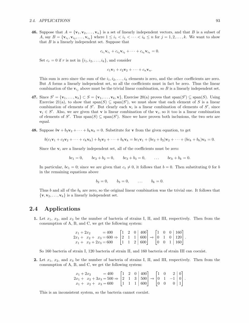
2.4. APPLICATIONS 93
46. Suppose that A = {v1,v2, . . . ,vn} is a set of linearly independent vectors, and that B is a subset ofA, say B = {vi1 ,vi2 , . . . ,vik} where 1 ≤ i1 < i1 < · · · < ik ≤ n for j = 1, 2, . . . , k. We want to showthat B is a linearly independent set. Suppose that
ci1vi1 + ci2vi2 + · · ·+ cikvik = 0.
Set cr = 0 if r is not in {i1, i2, . . . , ik}, and consider
c1v1 + c2v2 + · · ·+ cnvn.
This sum is zero since the sum of the i1, i2, . . . , ik elements is zero, and the other coefficients are zero.But A forms a linearly independent set, so all the coefficients must in fact be zero. Thus the linearcombination of the vij above must be the trivial linear combination, so B is a linearly independent set.
47. Since S′ = {v1, . . . ,vk} ⊂ S = {v1, . . . ,vk,v}, Exercise 20(a) proves that span(S′) ⊆ span(S). UsingExercise 21(a), to show that span(S) ⊆ span(S′), we must show that each element of S is a linearcombination of elements of S′. But clearly each vi is a linear combination of elements of S′, sincevi ∈ S′. Also, we are given that v is linear combination of the vi, so it too is a linear combinationof elements of S′. Thus span(S) ⊆ span(S′). Since we have proven both inclusions, the two sets areequal.
48. Suppose bv + b2v2 + · · ·+ bkvk = 0. Substitute for v from the given equation, to get
b(c1v1 + c2v2 + · · ·+ ckvk) + b2v2 + · · ·+ bkvk = bc1v1 + (bc2 + b2)v2 + · · ·+ (bck + bk)vk = 0.
Since the vi are a linearly independent set, all of the coefficients must be zero:
bc1 = 0, bc2 + b2 = 0, bc3 + b3 = 0, . . . bck + bk = 0.
In particular, bc1 = 0; since we are given that c1 6= 0, it follows that b = 0. Then substituting 0 for bin the remaining equations above
b2 = 0, b3 = 0, . . . bk = 0.
Thus b and all of the bk are zero, so the original linear combination was the trivial one. It follows that{v,v2, . . . ,vk} is a linearly independent set.
2.4 Applications
1. Let x1, x2, and x3 be the number of bacteria of strains I, II, and III, respectively. Then from theconsumption of A, B, and C, we get the following system:
x1 + 2x2 = 4002x1 + x2 + x3 = 600x1 + x2 + 2x3 = 600
⇒
1 2 0 4002 1 1 6001 1 2 600
−→1 0 0 160
0 1 0 1200 0 1 160
.So 160 bacteria of strain I, 120 bacteria of strain II, and 160 bacteria of strain III can coexist.
2. Let x1, x2, and x3 be the number of bacteria of strains I, II, and III, respectively. Then from theconsumption of A, B, and C, we get the following system:
x1 + 2x2 = 4002x1 + x2 + 3x3 = 500x1 + x2 + x3 = 600
⇒
1 2 0 4002 1 3 5001 1 1 600
−→1 0 2 0
0 1 −1 00 0 0 1
.This is an inconsistent system, so the bacteria cannot coexist.

94 CHAPTER 2. SYSTEMS OF LINEAR EQUATIONS
3. Let x1, x2, and x3 be the number of small, medium, and large arrangements. Then from the consump-tion of flowers in each arrangement we get:
x1 + 2x2 + 4x3 = 243x1 + 4x2 + 8x3 = 503x1 + 6x2 + 6x3 = 48
⇒
1 2 4 243 4 8 503 6 6 48
−→1 0 0 2
0 1 0 30 0 1 4
.So 2 small, 3 medium, and 4 large arrangements were sold that day.
4. (a) Let x1, x2, and x3 be the number of nickels, dimes, and quarters. Then we get
x1 + x2 + x3 = 202x1 − x2 = 05x1 + 10x2 + 25x3 = 300
⇒
1 1 1 202 −1 0 05 10 25 300
−→1 0 0 4
0 1 0 80 0 1 8
.So there are 4 nickels, 8 dimes, and 8 quarters.
(b) This is similar to part (a), except that the constraint 2x1 − x2 no longer applies, so we get[1 1 1 205 10 25 300
]−→[1 0 −3 −200 1 4 40
].
The general solution is x1 = −20 + 3t, x2 = 40− 4t, and x3 = t. From the first equation, we musthave 3t− 20 ≥ 0, so that t ≥ 7. From the second, we have t ≤ 10. So the possible values for t are7, 8, 9, and 10, which give the following combinations of nickels, dimes, and quarters:
[x1, x2, x3] = [1, 12, 7] or [4, 8, 8] or [7, 4, 9] or [10, 0, 10].
5. Let x1, x2, and x3 be the number of house, special, and gourmet blends. Then from the consumptionof beans in each blend we get
300x1 + 200x2 + 100x3 = 30,000200x2 + 200x3 = 15,000
200x1 + 100x2 + 200x3 = 25,000 .
Forming the augmented matrix and reducing it gives300 200 100 300000 200 200 15000
200 100 200 25000
−→1 0 0 65
0 1 0 300 0 1 45
.The merchant should make 65 house blend, 30 special blend, and 45 gourmet blend.
6. Let x1, x2, and x3 be the number of house, special, and gourmet blends. Then from the consumptionof beans in each blend we get
300x1 + 200x2 + 100x3 = 30,00050x1 200x2 + 350x3 = 15,000
150x1 + 100x2 + 50x3 = 15,000 .
Forming the augmented matrix and reducing it gives300 200 100 3000050 200 350 15000150 100 50 15000
−→1 0 −1 60
0 1 2 600 0 0 0
.Thus x1 = 60 + t, x2 = 60− 2t, and x3 = t. From the first equation, we get t ≥ −60; from the second,we get t ≤ 30, and the third gives us t ≥ 0. So the range of possible values is 0 ≤ t ≤ 30. We wish tomaximize the profit
P =1
2x1 +
3
2x2 + 2x3 =
1
2(60 + t) +
3
2(60− t) + 2t = 120− 1
2t.
Since 0 ≤ t ≤ 30, the profit is maximized if t = 0, in which case x1 = x+ 2 = 60 and x3 = 0. Thereforethe merchant should make 60 house and special blends, and no gourmet blends.

2.4. APPLICATIONS 95
7. Let x, y, z, and w be the number of FeS2, O2, Fe2O3, and SO2 molecules respectively. Then comparethe number of iron, sulfur, and oxygen atoms in reactants and products:
Iron: x = 2z
Sulfur: 2x = w
Oxygen: 2y = 3z + 2w,
so we get the matrix 1 0 −2 0 0
2 0 0 −1 0
0 2 −3 −2 0
−→1 0 0 − 1
2 0
0 1 0 − 118 0
0 0 1 − 14 0
.Thus z = 1
4w, y = 118 w, and x = 1
2w. The smallest positive value of w that will produce integer valuesfor all four variables is 8, so letting w = 8 gives x = 4, y = 11, z = 2, and w = 8. The balancedequation is 4FeS2 + 11O2 −→ 2Fe2O3 + 8SO2.
8. Let x, y, z, and w be the number of CO2, H2O, C6H12O6, and O2 molecules respectively. The comparethe number of carbon, oxygen, and hydrogen atoms in reactants and products:
Carbon: x = 6z
Oxygen: 2x+ y = 6z + 2w
Hydrogen: 2y = 12z.
This system is easy to solve using back-substitution: the first equation gives x = 6z and the third givesy = 6z. Substituting 6z for both x and y in the second equation gives 2 · 6z + 6z = 6z + 2w, so thatw = 6z as well. The smallest positive value of z giving integers is z = 1, so that x = y = w = 6 andz = 1. The balanced equation is 6CO2 + 6H2O −→ C6H12O6 + 6O2.
9. Let x, y, z, and w be the number of C4H10, O2, CO2, and H2O molecules respectively. The comparethe number of carbon, oxygen, and hydrogen atoms in reactants and products:
Carbon: 4x = z
Oxygen: 2y = 2z + w
Hydrogen: 10x = 2w.
This system is easy to solve using back-substitution: the first equation gives z = 4x and the third givesw = 5x. Substituting these values for z and w in the second equation gives 2y = 2 · 4x+ 5x = 13x, sothat y = 13
2 x. The smallest positive value of x giving integers for all four variables is x = 2, resultingin x = 2, y = 13, z = 8, and w = 10. The balanced equation is 2C4H10 + 13O2 −→ 8CO2 + 10H2O.
10. Let x, y, z, and w be the number of C7H6O2, O2, H2O, and CO2 molecules respectively. The comparethe number of carbon, oxygen, and hydrogen atoms in reactants and products:
Carbon: 7x = w
Oxygen: 2x+ 2y = z + 2w
Hydrogen: 6x = 2z.
This system is easy to solve using back-substitution: the first equation gives w = 7x and the thirdgives z = 3x. Substituting these values for w and z in the second equation gives 2x+ 2y = 3x+ 2 · 7x,so that y = 15
2 x. The smallest positive value for x giving integer values for all four variables isx = 2, so that the solution is x = 2, y = 15, z = 6, and w = 14. The balanced equation is2C7H6O2 + 15O2 −→ 6H2O+14CO2.

96 CHAPTER 2. SYSTEMS OF LINEAR EQUATIONS
11. Let x, y, z, and w be the number of C5H11OH, O2, H2O, and CO2 molecules respectively. The comparethe number of carbon, oxygen, and hydrogen atoms in reactants and products:
Carbon: 5x = w
Oxygen: x+ 2y = z + 2w
Hydrogen: 12x = 2z.
This system is easy to solve using back-substitution: the first equation gives w = 5x and the thirdgives z = 6x. Substituting these values for w and z in the second equation gives x+ 2y = 6x+ 2 · 5x,so that y = 15
2 x. The smallest positive value for x giving integer values for all four variables isx = 2, so that the solution is x = 2, y = 15, z = 12, and w = 10. The balanced equation is2C5H11OH+15O2 −→ 12H2O+10CO2.
12. Let x, y, z, and w be the number of HClO4, P4O10, H3PO4, and Cl2O7 molecules respectively. Thecompare the number of hydrogen, chlorine, oxygen, and phosphorus atoms in reactants and products:
Hydrogen: x = 3z
Chlorine: x = 2w
Oxygen: 4x+ 10y = 4z + 7w
Phosphorus: 4y = z.
This gives the matrix 1 0 −3 0 0
1 0 0 −2 0
4 10 −4 −7 0
0 4 −1 0 0
−→
1 0 0 −2 0
0 1 0 − 16 0
0 0 1 − 23 0
0 0 0 0 0
.Thus the general solution is x = 2t, y = 1
6 t, z = 23 t, w = t. The smallest positive value of t giving all
integer answers is t = 6, so the desired solution is x = 12, y = 1, z = 4, and w = 6. The balancedequation is 12HClO4+P4O10 −→ 4H3PO4 + 6Cl2O7.
13. Let x1, x2, x3, x4, and x5 be the number of Na2CO3, C, N2, NaCN, and CO molecules respectively.The compare the number of sodium, carbon, oxygen, and nitrogen atoms in reactants and products:
Sodium: 2x1 = x4
Carbon: x1 + x2 = x4 + x5
Oxygen: 3x1 = x5
Nitrogen: 2x3 = x4.
This gives the matrix 2 0 0 −1 0 0
1 1 0 −1 −1 0
3 0 0 0 −1 0
0 0 2 −1 0 0
−→
1 0 0 0 − 13 0
0 1 0 0 − 43 0
0 0 1 0 − 13 0
0 0 0 1 − 23 0
Thus x5 is a free variable, and
x1 =1
3x5, x2 =
4
3x5, x3 =
1
3x5, x4 =
2
3x5.
The smallest value of x5 that produces integer solutions is 3, so the desired solution is x1 = 1, x2 = 4,x3 = 1, x4 = 2, and x5 = 3. The balanced equation is Na2CO3 + 4C+N2 −→ 2NaCN+3CO.
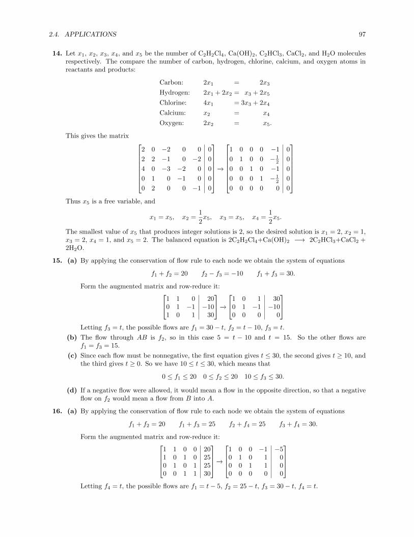
2.4. APPLICATIONS 97
14. Let x1, x2, x3, x4, and x5 be the number of C2H2Cl4, Ca(OH)2, C2HCl3, CaCl2, and H2O moleculesrespectively. The compare the number of carbon, hydrogen, chlorine, calcium, and oxygen atoms inreactants and products:
Carbon: 2x1 = 2x3
Hydrogen: 2x1 + 2x2 = x3 + 2x5
Chlorine: 4x1 = 3x3 + 2x4
Calcium: x2 = x4
Oxygen: 2x2 = x5.
This gives the matrix 2 0 −2 0 0 0
2 2 −1 0 −2 0
4 0 −3 −2 0 0
0 1 0 −1 0 0
0 2 0 0 −1 0
−→
1 0 0 0 −1 0
0 1 0 0 − 12 0
0 0 1 0 −1 0
0 0 0 1 − 12 0
0 0 0 0 0 0
Thus x5 is a free variable, and
x1 = x5, x2 =1
2x5, x3 = x5, x4 =
1
2x5.
The smallest value of x5 that produces integer solutions is 2, so the desired solution is x1 = 2, x2 = 1,x3 = 2, x4 = 1, and x5 = 2. The balanced equation is 2C2H2Cl4+Ca(OH)2 −→ 2C2HCl3+CaCl2 +2H2O.
15. (a) By applying the conservation of flow rule to each node we obtain the system of equations
f1 + f2 = 20 f2 − f3 = −10 f1 + f3 = 30.
Form the augmented matrix and row-reduce it:1 1 0 200 1 −1 −101 0 1 30
−→1 0 1 30
0 1 −1 −100 0 0 0
Letting f3 = t, the possible flows are f1 = 30− t, f2 = t− 10, f3 = t.
(b) The flow through AB is f2, so in this case 5 = t − 10 and t = 15. So the other flows aref1 = f3 = 15.
(c) Since each flow must be nonnegative, the first equation gives t ≤ 30, the second gives t ≥ 10, andthe third gives t ≥ 0. So we have 10 ≤ t ≤ 30, which means that
0 ≤ f1 ≤ 20 0 ≤ f2 ≤ 20 10 ≤ f3 ≤ 30.
(d) If a negative flow were allowed, it would mean a flow in the opposite direction, so that a negativeflow on f2 would mean a flow from B into A.
16. (a) By applying the conservation of flow rule to each node we obtain the system of equations
f1 + f2 = 20 f1 + f3 = 25 f2 + f4 = 25 f3 + f4 = 30.
Form the augmented matrix and row-reduce it:1 1 0 0 201 0 1 0 250 1 0 1 250 0 1 1 30
−→
1 0 0 −1 −50 1 0 1 00 0 1 1 00 0 0 0 0
Letting f4 = t, the possible flows are f1 = t− 5, f2 = 25− t, f3 = 30− t, f4 = t.

98 CHAPTER 2. SYSTEMS OF LINEAR EQUATIONS
(b) If f4 = t = 10, then the average flows on the other streets will be f1 = 10−5 = 5, f2 = 25−10 = 15,and f3 = 30− 10 = 20.
(c) Each flow must be nonnegative, so we get the constraints t ≥ 5, t ≤ 25, t ≤ 30, and t ≥ 0. Thus5 ≤ t ≤ 25. This gives the constraints
0 ≤ f1 ≤ 20 0 ≤ f2 ≤ 20 5 ≤ f3 ≤ 25 5 ≤ f4 ≤ 25.
(d) Reversing all of the directions would have no effect on the solution. This would mean multiplyingall rows of the augmented matrix by −1. However, multiplying a row by −1 is an elementary rowoperation, so the new matrix would have the same reduced row echelon form and thus the samesolution.
17. (a) By applying the conservation of flow rule to each node we obtain the system of equations
f1 + f2 = 100 f2 + f3 = f4 + 150 f4 + f5 = 150 f1 + 200 = f3 + f5.
Rearrange the equations, set up the augmented matrix, and row reduce it:1 1 0 0 0 1000 1 1 −1 0 1500 0 0 1 1 1501 0 −1 0 −1 −200
−→
1 0 −1 0 −1 −2000 1 1 0 1 3000 0 0 1 1 1500 0 0 0 0
Then both f3 = s and f5 = t are free variables, so the flows are
f1 = −200 + s+ t, f2 = 300− s− t, f3 = s, f4 = 150− t, f5 = t.
(b) If DC is closed, then f5 = t = 0, so that f1 = −200 + s and f2 = 300 − s. Thus s, which is theflow through DB, must satisfy 200 ≤ s ≤ 300 liters per day.
(c) If DB = f3 = S were closed, then f1 = −200 + t, so that t = f5 ≥ 200. But that would meanthat f4 = 150− t ≤ −50 < 0, which is impossible.
(d) Since f4 = 150− t, we must have 0 ≤ t ≤ 150, so that 0 ≤ f4 ≤ 150. Note that all of these valuesfor t are consistent with the first three equations as well: if t = 0, then s = 250 produces positivevalues for all flows, while if t = 150, then s = 75 produces all positive values. So the flow throughDB is between 0 and 150 liters per day.
18. (a) By applying the conservation of flow rule to each node we obtain:
f3 + 200 = f1 + 100 f1 + 150 = f2 + f4 f2 + f5 = 300
f6 + 100 = f3 + 200 f4 + f7 = f6 + 100 f5 + f7 = 250.
Create and row-reduce the augmented matrix for the system:1 0 −1 0 0 0 0 1001 −1 0 −1 0 0 0 −1500 1 0 0 1 0 0 3000 0 1 0 0 −1 0 −1000 0 0 1 0 −1 1 1000 0 0 0 1 0 1 250
−→
1 0 0 0 0 −1 0 00 1 0 0 0 0 −1 500 0 1 0 0 −1 0 −1000 0 0 1 0 −1 1 1000 0 0 0 1 0 1 2500 0 0 0 0 0 0 0
Let f7 = t and f6 = s, so the flows are
f1 = s f2 = 50 + t f3 = −100 + s f4 = 100 + s− t f5 = 250− t f6 = s f7 = t.
(b) From the solution in part (a), since f1 = s = f6, it is not possible for f1 and f6 to have differentvalues.

2.4. APPLICATIONS 99
(c) If f4 = 0, then s− t = 100, so that t = 100 + s. Substituting this for t everywhere gives
f1 = s f2 = 150 + s f3 = −100 + s f4 = 0 f5 = 150− s f6 = s f7 = 100 + s.
The constraints imposed by the requirement that all the fi be nonnegative means that 100 ≤ s ≤150, so that
100 ≤ f1 ≤ 150 250 ≤ f2 ≤ 300 0 ≤ f3 ≤ 50 f4 = 0
50 ≤ f5 ≤ 100 100 ≤ f6 ≤ 150 200 ≤ f7 ≤ 250.
19. Applying the current law to node A gives I1 + I3 = I2 or I1 − I2 + I3 = 0. Applying the voltagelaw to the top circuit, ABCA, gives −I2 − I1 + 8 = 0. Similarly, for the circuit ABDA we obtain−I2 + 13− 4I3 = 0. This gives the system
I1 − I2 + I3 = 0I1 + I2 = 8
I2 + 4I3 = 13⇒
1 −1 1 01 1 0 80 1 4 13
−→1 0 0 3
0 1 0 50 0 1 2
Thus I1 = 3 amps, I2 = 5 amps, and I3 = 2 amps.
20. Applying the current law to node B and the voltage law to the upper and lower circuits gives
I1 − I2 + I3 = 0I1 + 2I2 = 5
2I2 + 4I3 = 8⇒
1 −1 1 01 2 0 50 2 4 8
−→1 0 0 1
0 1 0 20 0 1 1
Thus I1 = 1 amps, I2 = 2 amps, and I3 = 1 amp.
21. (a) Applying the current and voltage laws to the circuit gives the system:
Node B: I = I1 + I4
Node C: I1 = I2 + I3
Node D: I2 + I5 = I
Node E: I3 + I4 = I5
Circuit ABEDA: −2I4 − I5 + 14 = 0
Circuit BCEB: −I1 − I3 + 2I4 = 0
Circuit CDEC: −2I2 + I3 + I5 = 0
Construct the augmented matrix and row-reduce it:
1 −1 0 0 −1 0 00 1 −1 −1 0 0 01 0 −1 0 0 −1 00 0 0 1 1 −1 00 0 0 0 2 1 140 1 0 1 −2 0 00 0 2 −1 0 −1 0
−→
1 0 0 0 0 0 100 1 0 0 0 0 60 0 1 0 0 0 40 0 0 1 0 0 20 0 0 0 1 0 40 0 0 0 0 1 60 0 0 0 0 0 0
Thus the currents are I = 10, I1 = 6, I2 = 4, I3 = 2, I4 = 4, and I5 = 6 amps.
(b) From Ohm’s Law, the effective resistance is Reff = VI = 14
10 = 75 ohms.
(c) To force the current in CE to be zero, we force I3 = 0 and let r be the resistance in BC. This

100 CHAPTER 2. SYSTEMS OF LINEAR EQUATIONS
gives the following system of equations:
Node B: I = I1 + I4
Node C: I1 = I2
Node D: I2 + I5 = I
Node E: I4 = I5
Circuit ABEDA: −2I4 − I5 + 14 = 0
Circuit BCEB: −rI1 + 2I4 = 0
Circuit CDEC: −2I2 + I5 = 0
It is easier to solve this system by substitution. Substitute I4 = I5 in the circuit equation forABEDA to get −3I5 + 14 = 0, so that I4 = I5 = 14
3 . Thus −2I2 + 143 = 0 so that I1 = I2 = 7
3 .Then the circuit equation for BCED gives us
−r · 7
3+ 2 · 14
3= 0 ⇒ r = 4.
So if we use a 4 ohm resistor in BC, the current in CE will be zero.
22. (a) Applying the voltage law to Figure 2.23(a) gives IR1+IR2 = E. But from Ohm’s Law, E = IReff ,so that I(R1 +R2) = IReff and thus Reff = R1 +R2.
(b) Applying the current and voltage laws to Figure 2.23(b) gives the system of equations I = I1 +I2,−I1R1 + I2R2 = 0, −I1R1 + E = 0, and −I2R2 + E = 0. Gauss-Jordan elimination gives
1 −1 −1 0
0 −R1 R2 0
0 −R1 0 −E0 0 −R2 −E
−→
1 0 0 (R1+R2)ER1R2
0 1 0 ER1
0 0 1 ER2
0 0 0 0
.
Thus I = (R1+R2)ER1R2
, I1 = ER1
, I2 = ER2
. But E = IReff ; substituting this value of E into theequation for I gives
I =(R1 +R2)IReff
R1R2⇒ Reff =
1R1+R2
R1R2
=1
1R1
+ 1R2
.
23. The matrix for this system, with inputs on the left, outputs along the top, is
Farming Manufacturing
Farming 12
13
Manufacturing 12
23
Let the output of the farm sector be f and the output of the manufacturing sector be m. Then
1
2f +
1
3m = f
1
2f +
2
3m = m.
Simplifying and row-reducing the corresponding augmented matrix gives
− 12f + 1
3m= 012f −
13m= 0
⇒
[− 1
213 0
12 − 1
3 0
]−→
[1 − 2
3 0
0 0 0
]
Thus f = 23m, so that farming and manufacturing must be in a 2 : 3 ratio.

2.4. APPLICATIONS 101
24. The matrix for this system, with needed resources on the left, outputs along the top, is
Coal SteelCoal 0.3 0.8Steel 0.7 0.2
Let the coal output be c and the steel output be s. Then
0.3c+ 0.8s = c
0.7c+ 0.2s = s.
Simplifying and row-reducing the corresponding augmented matrix gives
−0.7c + 0.8s = 00.7c − 0.8s = 0
⇒[−0.7 0.8 0
0.7 −0.8 0
]−→[1 − 8
7 00 0 0
]Thus c = 8
7s, so that coal and steel must be in an 8 : 7 ratio. For a total output of $20 million, coaloutput must be 8
8+7 · 20 = 323 ≈ $10.667 million, while steel output is 7
8+7 · 20 = 283 ≈ $9.333 million.
25. Let x be the painter’s rate, y the plumber’s rate, and z the electrician’s rate. From the given schedule,we get the linear system
2x+ y + 5z = 10x
4x+ 5y + z = 10y
4x+ 4y + 4z = 10z.
Simplifying and row-reducing the corresponding augmented matrix gives
−8x+ y + 5z = 0
4x− 5y + z = 0
4x+ 4y − 6z = 0
⇒
−8 1 5 0
4 −5 1 0
4 4 −6 0
−→1 0 − 13
18 0
0 1 − 79 0
0 0 0 0
.Thus x = 13
18z and y = 79z. Let z = 54; this is a whole number in the required range such that the
others will be whole numbers as well. Then x = 39 and y = 42. The painter should charge $39 perhour, the plumber $42 per hour, and the electrician $54 per hour.
26. From the given matrix, we get the linear system
1
4L+
1
8T +
1
6Z = B
1
2B +
1
4L+
1
4T +
1
6Z = L
1
4B +
1
4L+
1
2T +
1
3Z = T
1
4B +
1
4L+
1
8T +
1
3Z = Z.
Simplify and row-reduce the associated augmented matrix:
−B + 14L+ 1
8T + 16Z = 0
12B −
34L+ 1
4T + 16Z = 0
14B + 1
2L−12T + 1
3Z = 014B + 1
8L+ 18T −
23Z = 0
⇒
−1 1
418
16 0
12 − 3
414
16 0
14
12 − 1
213 0
14
18
18 − 2
3 0
−→
1 0 0 − 23 0
0 1 0 − 65 0
0 0 1 − 85 0
0 0 0 0 0
.Thus B = 2
3Z, L = 65Z, and T = 8
5Z. Furthermore, B is the smallest price of the four, so B = 23Z
must be at least 50, in which case Z = 75. With that value of Z, we get B = 50, L = 90, and T = 120.

102 CHAPTER 2. SYSTEMS OF LINEAR EQUATIONS
27. The matrix for this system, with needed resources on the left, outputs along the top, is
Coal SteelCoal 0.15 0.2Steel 0.1 0.1
(a) Let the coal output be c and the steel output be s. Then since 45 million of external demand isrequired for coal and 124 million for steel, we have
c = 0.15c+ 0.25s+ 45
s = 0.2c+ 0.1s+ 124.
Simplify and row-reduce the associated matrix:
0.85c − 0.25s = 45−0.2c + 0.9s + 124
⇒[
0.85 −0.25 45−0.2 0.9 124
]−→[1 0 1000 1 160
]So the coal industry should produce $100 million and the steel industry should produce $160million.
(b) The new external demands for coal and steel are 40 and 130 million respectively. The only thingthat changes in the equations is the constant terms, so we have
0.85c − 0.25s = 40−0.2c + 0.9s + 130
⇒[
0.85 −0.25 40−0.2 0.9 130
]−→[1 0 95.80 1 165.73
]So the coal industry should reduce production by 100−95.8 = $4.2 million, while the steel industryshould increase production by 165.73− 160 = $5.73 million.
28. This is an open system with external demand given by the other city departments. From the givenmatrix, we get the system
1 + 0.2A+ 0.1H + 0.2T = A
1.2 + 0.1A+ 0.1H + 0.2T = H
0.8 + 0.2A+ 0.4H + 0.3T = T .
Simplifying and row-reducing the associated augmented matrix gives
0.8A − 0.1H − 0.2T = 1−0.1A + 0.9H − 0.2T = 1.2−0.2A − 0.4H + 0.7T = 0.8
⇒
0.8 −0.1 −0.2 1−0.1 0.9 −0.2 1.2−0.2 −0.4 0.7 0.8
−→1 0 0 2.31
0 1 0 2.280 0 1 3.11
.So the Administrative department should produce $2.31 million of services, the Health department$2.28 million, and the Transportation department $3.11 million.
29. (a) Over Z2, we need to solve x1a + x2b + · · ·+ x5e = t + s:
s =
00000
, t =
01010
, ⇒
1 1 0 0 0 01 1 1 0 0 10 1 1 1 0 00 0 1 1 1 10 0 0 1 1 0
−→
1 0 0 0 1 10 1 0 0 1 10 0 1 0 0 10 0 0 1 1 00 0 0 0 0 0
Hence x5 is a free variable, so there are exactly two solutions (with x5 = 0 and with x5 = 1).Solving for the other variables, we get x1 = 1 + x5, x2 = 1 + x5, x3 = 1, and x4 = x5. So the twosolutions are
x1
x2
x3
x4
x5
=
11100
,x1
x2
x3
x4
x5
=
00111
.So we can push switches 1, 2, and 3 or switches 3, 4, and 5.
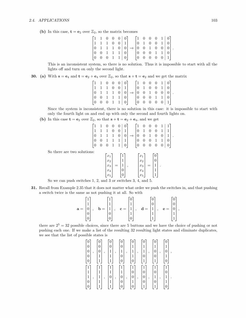
2.4. APPLICATIONS 103
(b) In this case, t = e2 over Z2, so the matrix becomes1 1 0 0 0 01 1 1 0 0 10 1 1 1 0 00 0 1 1 1 00 0 0 1 1 0
−→
1 0 0 0 1 00 1 0 0 1 00 0 1 0 0 00 0 0 1 1 00 0 0 0 0 1
.This is an inconsistent system, so there is no solution. Thus it is impossible to start with all thelights off and turn on only the second light.
30. (a) With s = e4 and t = e2 + e4 over Z2, so that s + t = e2 and we get the matrix1 1 0 0 0 01 1 1 0 0 10 1 1 1 0 00 0 1 1 1 00 0 0 1 1 0
−→
1 0 0 0 1 00 1 0 0 1 00 0 1 0 0 00 0 0 1 1 00 0 0 0 0 1
.Since the system is inconsistent, there is no solution in this case: it is impossible to start withonly the fourth light on and end up with only the second and fourth lights on.
(b) In this case t = e2 over Z2, so that s + t = e2 + e4, and we get1 1 0 0 0 01 1 1 0 0 10 1 1 1 0 00 0 1 1 1 10 0 0 1 1 0
−→
1 0 0 0 1 10 1 0 0 1 10 0 1 0 0 10 0 0 1 1 00 0 0 0 0 0
.So there are two solutions:
x1
x2
x3
x4
x5
=
11100
,x1
x2
x3
x4
x5
=
00111
.So we can push switches 1, 2, and 3 or switches 3, 4, and 5.
31. Recall from Example 2.35 that it does not matter what order we push the switches in, and that pushinga switch twice is the same as not pushing it at all. So with
a =
11000
, b =
11100
, c =
01110
, d =
00111
, e =
00011
,there are 25 = 32 possible choices, since there are 5 buttons and we have the choice of pushing or notpushing each one. If we make a list of the resulting 32 resulting light states and eliminate duplicates,we see that the list of possible states is
00000
,
00011
,
00111
,
00100
,
01110
,
01101
,
01001
,
01010
,
11100
,
11111
,
11011
,
11000
,
10010
,
10001
,
10101
,
10110
.
104 CHAPTER 2. SYSTEMS OF LINEAR EQUATIONS
32. (a) Over Z3, we need to solve x1a + x2b + x3c = t, where
t =
021
, so that
1 1 0 01 1 1 20 1 1 1
−→1 0 0 1
0 1 0 20 0 1 2
.Thus x1 = 1, x2 = 2, and x3 = 2, so we must push switch A once and switches B and C twiceeach.
(b) Over Z3, we need to solve x1a + x2b + x3c = t, where
t =
101
, so that
1 1 0 11 1 1 00 1 1 1
−→1 0 0 2
0 1 0 20 0 1 2
.In other words, we must push each switch twice.
(c) Let x, y, and z be the final states of the three lights. Then we want to solve1 1 0 x1 1 1 y0 1 1 z
−→1 0 0 y + 2z
0 1 0 x+ 2y + z0 0 1 2x+ y
.So we can achieve this configuration if we push switch A y+ 2z times, switch B x+ 2y+ z times,and switch C 2x+ y times (adding in Z3).
33. The switches here correspond to the same vectors as in Example 2.35, but now the numbers areinterpreted in Z3 rather than in Z2. So in Z5
3, with s = 0 (all lights initially off), we need to solvex1a + x2b + · · ·+ x5e = t, where
t =
21212
, so that
1 1 0 0 0 21 1 1 0 0 10 1 1 1 0 20 0 1 1 1 10 0 0 1 1 2
−→
1 0 0 0 1 10 1 0 0 2 10 0 1 0 0 20 0 0 1 1 20 0 0 0 0 0
So x5 is a free variable, so there are three solutions, corresponding to x5 = 0, 1, or 2. Solving for theother variables gives
x1 = 1− x5, x2 = 1− 2x5, x3 = 2, x4 = 2− x5,
so that the solutions are (remembering that 1− 2 = 2 and 2 · 2 = 1 in Z3)x1
x2
x3
x4
x5
=
11220
,
02211
,
20202
.
34. The possible configurations are1 1 0 0 01 1 1 0 00 1 1 1 00 0 1 1 10 0 0 1 1
s1
s2
s3
s4
s5
=
s1 + s2
s1 + s2 + s3
s2 + s3 + s4
s3 + s4 + s5
s4 + s5
where si ∈ {0, 1, 2} is the number of times that switch i is thrown.

2.4. APPLICATIONS 105
35. (a) Let a value of 1 represent white, and 0 represent black. Let ai correspond to touching the numberi; it has a 1 in a given entry if the value of that square changes when i is pressed, and a 0 if it doesnot (thus the 1’s correspond to the squares with the blue dots in them in the diagram). Sinceeach square has two states, white and black, we need to solve, over Z2, the equation
s + x1a1 + x2a2 + · · ·+ x9a9 = t.
Here
s =
011101110
, t =
000000000
, so that x1a1 + x2a2 + · · ·+ x9a9 = 0− s = s.
Row-reducing the corresponding augmented matrix gives
1 1 0 1 0 0 0 0 0 01 1 1 0 1 0 0 0 0 10 1 1 0 0 1 0 0 0 11 0 0 1 1 0 1 0 0 11 0 1 0 1 0 1 0 1 00 0 1 0 1 1 0 0 1 10 0 0 1 0 0 1 1 0 10 0 0 0 1 0 1 1 1 10 0 0 0 0 1 0 1 1 0
−→
1 0 0 0 0 0 0 0 0 00 1 0 0 0 0 0 0 0 00 0 1 0 0 0 0 0 0 10 0 0 1 0 0 0 0 0 00 0 0 0 1 0 0 0 0 00 0 0 0 0 1 0 0 0 00 0 0 0 0 0 1 0 0 10 0 0 0 0 0 0 1 0 00 0 0 0 0 0 0 0 1 0
.
So touching the third and seventh squares will turn all the squares black.
(b) In part (a), note that the row-reduced matrix consists of the identity matrix and a column vectorcorresponding to the constants. Changing the constants cannot produce an inconsistent system,since the matrix will still reduce to the identity matrix. So any configuration is reachable, sincewe can solve x1a1 + x2a2 + · · ·+ x9a9 = s for any s.
36. In this version of the puzzle, the squares have three states, so we work over Z3, with 2 correspondingto black, 1 to gray, and 0 to white. Then we need to go from
s =
220110201
to t =
222222222
.
Thus we want to solve
x1a1 + x2a2 + · · ·+ x9a9 = t− s =
002112021
.

106 CHAPTER 2. SYSTEMS OF LINEAR EQUATIONS
Row-reducing the corresponding augmented matrix gives
1 1 0 1 0 0 0 0 0 01 1 1 0 1 0 0 0 0 00 1 1 0 0 1 0 0 0 21 0 0 1 1 0 1 0 0 11 0 1 0 1 0 1 0 1 10 0 1 0 1 1 0 0 1 20 0 0 1 0 0 1 1 0 00 0 0 0 1 0 1 1 1 20 0 0 0 0 1 0 1 1 1
−→
1 0 0 0 0 0 0 0 0 00 1 0 0 0 0 0 0 0 10 0 1 0 0 0 0 0 0 00 0 0 1 0 0 0 0 0 20 0 0 0 1 0 0 0 0 20 0 0 0 0 1 0 0 0 10 0 0 0 0 0 1 0 0 00 0 0 0 0 0 0 1 0 10 0 0 0 0 0 0 0 1 2
,
showing that a solution exists.
37. Let Grace and Hans’ ages be g and h. Then g = 3h and g+ 5 = 2(h+ 5), or g = 2(h+ 5)− 5 = 2h+ 5.It follows that g = 3h = 2h+ 5, so that h = 5 and g = 15. So Hans is 5 and Grace is 15.
38. Let the ages be a, b, and c. Then the first two conditions give us a + b + c = 60 and a − b = b − c.For the third condition, Bert will be as old as Annie is now in a− b years; at that time, Annie will bea+ (a− b) = 2a− b years, and we are given that 2a− b = 3c. So we get the system
a + b + c = 60a − 2b + c = 0
2a − b − 3c = 0⇒
31 1 1 601 −2 1 02 −1 −3 0
−→31 0 0 28
0 1 0 200 0 1 12
.Annie is 28, Bert is 20, and Chris is 12.
39. Let the areas of the fields be a and b. We have the two equations
a+ b = 1800
2
3a+
1
2b = 1100.
Multiply the first equation by two and subtract the first equation from the result to get 13a = 400, so
that a = 1200 square yards and thus b = 1800− a = 600 square yards.
40. Let x1, x2, and x3 be the number of bundles of the first, second, and third types of corn. Then fromthe given conditions we get
3x1 + 2x2 + x3 = 39
2x1 + 3x2 + x3 = 34
x1 + 2x2 + 3x3 = 26.
Row-reduce the augmented matrix to get3 2 1 39
2 3 1 34
1 2 3 26
−→1 0 0 37
4
0 1 0 174
0 0 1 114
.Therefore there are 9.25 measures of corn in a bundle of the first type, 4.25 measures of corn in abundle of the second type, and 2.75 measures of corn in a bundle of the third type.
41. (a) The addition table gives a+ c = 2, a+ d = 4, b+ c = 3, b+ d = 5. Construct and row-reduce thecorresponding augmented matrix:
1 0 1 0 21 0 0 1 40 1 1 0 30 1 0 1 5
−→
1 0 0 1 40 1 0 1 50 0 1 −1 −20 0 0 0 0
.

2.4. APPLICATIONS 107
So d is a free variable. Solving for the other variables in terms of d gives a = 4− d, b = 5− d, andc = d − 2. So there are an infinite number of solutions; for example, with d = 1, we get a = 3,b = 4, and c = −1.
(b) We have a+ c = 3, a+ d = 4, b+ c = 6, b+ d = 5. Construct and row-reduce the correspondingaugmented matrix:
1 0 1 0 31 0 0 1 40 1 1 0 60 1 0 1 5
−→
1 0 0 1 00 1 0 1 00 0 1 −1 00 0 0 0 1
.So this is an inconsistent system, and there are no such values of a, b, c, and d.
42. The addition table gives a + c = w, a + d = y, b + c = x, b + d = z. Construct and row-reduce thecorresponding augmented matrix:
1 0 1 0 w1 0 0 1 y0 1 1 0 x0 1 0 1 z
−→
1 0 0 1 w0 1 0 1 x0 0 1 −1 y − w0 0 0 0 z − x− y + w
.In order for this to be a consistent system, we must have z−x− y+w = 0, or z− y = x−w. Anotherway of phrasing this is x+ y = z + w; in other words, the sum of the diagonal entries must equal thesum of the off-diagonal entries.
43. (a) The addition table gives the following system of equations:
a+ d = 3 b+ d = 2 c+ d = 1
a+ e = 5 b+ e = 4 c+ e = 3
a+ f = 4 b+ f = 3 c+ f = 1.
Construct and row-reduce the corresponding augmented matrix:
1 0 0 1 0 0 31 0 0 0 1 0 51 0 0 0 0 1 40 1 0 1 0 0 20 1 0 0 1 0 40 1 0 0 0 1 30 0 1 1 0 0 10 0 1 0 1 0 30 0 1 0 0 1 1
−→
1 0 0 0 0 1 00 1 0 0 0 1 00 0 1 0 0 1 00 0 0 1 0 −1 00 0 0 0 1 −1 00 0 0 0 0 0 10 0 0 0 0 0 00 0 0 0 0 0 00 0 0 0 0 0 0
.
The sixth row shows that this is an inconsistent system.
(b) The addition table gives the following system of equations:
a+ d = 1 b+ d = 2 c+ d = 3
a+ e = 3 b+ e = 4 c+ e = 5
a+ f = 4 b+ f = 5 c+ f = 6.
Construct and row-reduce the corresponding augmented matrix:
1 0 0 1 0 0 11 0 0 0 1 0 31 0 0 0 0 1 40 1 0 1 0 0 20 1 0 0 1 0 40 1 0 0 0 1 50 0 1 1 0 0 30 0 1 0 1 0 50 0 1 0 0 1 6
−→
1 0 0 0 0 1 40 1 0 0 0 1 50 0 1 0 0 1 60 0 0 1 0 −1 −30 0 0 0 1 −1 −10 0 0 0 0 0 00 0 0 0 0 0 00 0 0 0 0 0 00 0 0 0 0 0 0
.

108 CHAPTER 2. SYSTEMS OF LINEAR EQUATIONS
So f is a free variable, and there are an infinite number of solutions of the form a = 4 − f ,b = 5− f , c = 6, d = f − 3, e = f − 1.
44. Generalize the addition table to+ a b cd m n oe p q rf s t u
The addition table gives the following system of equations:
a+ d = m b+ d = n c+ d = o
a+ e = p b+ e = q c+ e = r
a+ f = s b+ f = t c+ f = u.
Construct and row-reduce the corresponding augmented matrix:
1 0 0 1 0 0 m1 0 0 0 1 0 p1 0 0 0 0 1 s0 1 0 1 0 0 n0 1 0 0 1 0 q0 1 0 0 0 1 t0 0 1 1 0 0 o0 0 1 0 1 0 r0 0 1 0 0 1 u
−→
1 0 0 0 0 1 m0 1 0 0 0 1 n0 0 1 0 0 1 o0 0 0 1 0 −1 m− p0 0 0 0 1 −1 n+ p−m− t0 0 0 0 0 0 m− n− p+ q0 0 0 0 0 0 n− o− q + r0 0 0 0 0 0 p− q − s+ t0 0 0 0 0 0 q − r − t+ u
.
For the table to be valid, the last entry in the zero rows must also be zero, so we need the conditionsm+ q = n+p, n+ r = o+ q, p+ t = q+ s, and q+u = r+ t. In terms of the addition table, this meansthat for each 2× 2 submatrix, the sum of the diagonal entries must equal the sum of the off-diagonalentries (compare with Exercise 42).
45. (a) Since the three points (0, 1), (−1, 4), and (2, 1) must satisfy the equation y = ax2 + bx + c,substitute those values to get the three equations c = 1, a − b + c = 4, and 4a + 2b + c = 1.Construct and row-reduce the corresponding augmented matrix:0 0 1 1
1 −1 1 44 2 1 1
−→1 0 0 1
0 1 0 −20 0 1 1
Thus a = 1, b = −2, and c = 1, so that the equation of the parabola is y = x2 − 2x+ 1.
(b) Since the three points (−3, 1), (−2, 2), and (−1, 5) must satisfy the equation y = ax2 + bx + c,substitute those values to get the three equations 9a−3b+c = 1, 4a−2b+c = 2, and a−b+c = 5.Construct and row-reduce the corresponding augmented matrix:9 −3 1 1
4 −2 1 21 1 1 5
−→1 0 0 1
0 1 0 60 0 1 10
Thus a = 1, b = 6, and c = 10, so that the equation of the parabola is y = x2 + 6x+ 10.
46. (a) Since the three points (0, 1), (−1, 4), and (2, 1) must satisfy the equation x2 +y2 +ax+by+c = 0,substitute those values to get the three equations
1 + b + c = 01 + 16 − a + 4b + c = 04 + 1 + 2a + b + c = 0
⇒b + c = −1
a − 4b − c = 172a + b + c = −5 .

2.4. APPLICATIONS 109
Construct and row-reduce the corresponding augmented matrix:0 1 1 −11 −4 −1 172 1 1 −5
−→1 0 0 −2
0 1 0 −60 0 1 5
Thus a = −2, b = −6, and c = 5, so that the equation of the circle is x2 + y2 − 2x− 6y + 5 = 0.Completing the square gives (x− 1)2 + (y − 3)2 + 5− 1− 9 = 0, so that (x− 1)2 + (y − 3)2 = 5.This is a circle whose center is (1, 3), with radius
√5. A sketch of the circle follows part (b).
(b) Since the three points (−3, 1), (−2, 2), and (−1, 5) must satisfy the equation x2+y2+ax+by+c = 0,substitute those values to get the three equations
9 + 1 − 3a + b + c = 04 + 4 − 2a + 2b + c = 01 + 25 − a + 5b + c = 0
⇒3a − b − c = 102a − 2b − c = 8a − 5b − c = 26 .
Construct and row-reduce the corresponding augmented matrix:3 −1 −1 102 −2 −1 81 −5 −1 26
−→1 0 0 12
0 1 0 −100 0 1 36
Thus a = 12, b = −10, and c = 36, so that the equation of the circle is x2 +y2 +12x−10y+36 = 0.Completing the square gives (x+6)2 +(y−5)2 +36−36−25 = 0, so that (x+6)2 +(y−5)2 = 25.This is a circle whose center is (−6, 5), with radius 5. Sketches of both circles are:
H0, 1L
H-1, 4L
H2, 1L
H1, 3L
-2 -1 1 2 3 4
1
2
3
4
5
6
H-3, 1L
H-2, 2L
H-1, 5LH-6, 5L
-11 -10 -9 -8 -7 -6 -5 -4 -3 -2 -1
1
2
3
4
5
6
7
8
9
10
47. We have 3x+1x2+2x−3 = 3x+1
(x−1)(x+3) = Ax−1 + B
x+3 , so that clearing fractions, we get (x+ 3)A+ (x− 1)B =
3x+ 1. Collecting terms gives (A+B)x+ (3A−B) = 3x+ 1. This gives the linear system A+B = 3,3A−B = 1. Construct and row-reduce the corresponding augmented matrix:[
1 1 33 −1 1
]−→[1 0 10 1 2
].
Thus A = 1 and B = 2, so that 3x+1x2+2x−3 = 1
x−1 + 2x+3 .
110 CHAPTER 2. SYSTEMS OF LINEAR EQUATIONS
48. We have
x2 − 3x+ 3
x3 + 2x2 + x=x3 − 3x+ 3
x(x+ 1)2=A
x+
B
x+ 1+
C
(x+ 1)2⇒
x2 − 3x+ 3 = A(x+ 1)2 +Bx(x+ 1) + Cx ⇒x2 − 3x+ 3 = (A+B)x2 + (2A+B + C)x+A ⇒
A+B = 1, 2A+B + C = −3, A = 3.
This is most easily solved by substitution: A = 3, so that A+B = 1 gives B = −2. Substituting intothe remaining equation gives 2 · 3− 2 + C = −3, so that C = −7. Thus
x2 − 3x+ 3
x3 + 2x2 + x=
3
x− 2
x+ 1− 7
(x+ 1)2
49. We have
x− 1
(x+ 1)(x2 + 1)(x2 + 4)=
A
x+ 1+Bx+ C
x2 + 1+Dx+ E
x2 + 4⇒
x− 1 = A(x2 + 1)(x2 + 4) + (Bx+ C)(x+ 1)(x2 + 4) + (Dx+ E)(x+ 1)(x2 + 1).
Expand the right-hand side and collect terms to get
x− 1 = (A+B +D)x4 + (B + C +D + E)x3 + (5A+ 4B + C +D + E)x2
+ (4B + 4C +D + E)x+ (4A+ 4C + E).
This gives the linear system
A+ B +D = 0
B + C +D + E = 0
5A+ 4B + C +D + E = 0
4B + 4C +D + E = 1
4A + 4C + E = −1.
Construct and row-reduce the corresponding augmented matrix:1 1 0 1 0 0
0 1 1 1 1 0
5 4 1 1 1 0
0 4 4 1 1 1
4 0 4 0 1 −1
−→
1 0 0 0 0 − 15
0 1 0 0 0 13
0 0 1 0 0 0
0 0 0 1 0 − 215
0 0 0 0 1 − 15
.
Thus A = − 15 , B = 1
3 , C = 0, D = − 215 , and E = − 1
5 , giving
x− 1
(x+ 1)(x2 + 1)(x2 + 4)= − 1
5(x+ 1)+
x
3(x2 + 1)−
215x+ 1
5
x2 + 4
= − 1
5(x+ 1)+
x
3(x2 + 1)− 2x+ 3
15(x2 + 4).
50. We have
x3 + x+ 1
x(x− 1)(x2 + x+ 1)(x2 + 1)3=A
x+
B
x− 1+
Cx+D
x2 + x+ 1+Ex+ F
x2 + 1+
Gx+H
(x2 + 1)2+
Ix+ J
(x2 + 1)3.

2.4. APPLICATIONS 111
Multiply both sides of the equation by x(x− 1)(x2 + x+ 1)(x2 + 1)3, simplify, and equate coefficientsof xn to get the system
A+B + C + E = 0 −3A+ 3B − 3C + 3D − 2E + F −G+H + J = 0
B − C +D + F = 0 A+ 4B + C − 3D − 2F −H = 1
3A+ 4B + 3C −D + 2E +G = 0 −3A+B − C +D − E −G− I = 0
−A+ 3B − 3C + 3D − E + 2F +H = 0 B −D − F −H − J = 1
3A+ 6B + 3C − 3D + E − F +G+ I = 0 −A = 1.
Construct and row-reduce the corresponding augmented matrix:
1 1 1 0 1 0 0 0 0 0 0
0 1 −1 1 0 1 0 0 0 0 0
3 4 3 −1 2 0 1 0 0 0 0
−1 3 −3 3 −1 2 0 1 0 0 0
3 6 3 −3 1 −1 1 0 1 0 0
−3 3 −3 3 −2 1 −1 1 0 1 0
1 4 1 −3 0 −2 0 −1 0 0 1
−3 1 −1 1 −1 0 −1 0 −1 0 0
0 1 0 −1 0 −1 0 −1 0 −1 1
−1 0 0 0 0 0 0 0 0 0 1
−→
1 0 0 0 0 0 0 0 0 0 −1
0 1 0 0 0 0 0 0 0 0 18
0 0 1 0 0 0 0 0 0 0 −1
0 0 0 1 0 0 0 0 0 0 0
0 0 0 0 1 0 0 0 0 0 158
0 0 0 0 0 1 0 0 0 0 − 98
0 0 0 0 0 0 1 0 0 0 74
0 0 0 0 0 0 0 1 0 0 − 14
0 0 0 0 0 0 0 0 1 0 12
0 0 0 0 0 0 0 0 0 1 12
.
This gives the partial fraction decomposition
x3 + x+ 1
x(x− 1)(x2 + x+ 1)(x2 + 1)3= − 1
x+
18
x− 1− x
x2 + x+ 1+
158 x−
98
x2 + 1+
74x−
14
(x2 + 1)2+
12x+ 1
2
(x2 + 1)3
= − 1
x+
1
8(x− 1)− x
x2 + 1+
15x− 9
8(x2 + 1)+
7x− 1
4(x2 + 1)2+
x+ 1
2(x2 + 1)3.
51. Suppose that 1 + 2 + · · ·+ n = an2 + bn+ c, and let n = 0, 1, and 2 to get the system
c = 0
a+ b+ c = 1
4a+ 2b+ c = 3.
Construct and row-reduce the associated augmented matrix:0 0 1 0
1 1 1 1
4 2 1 3
−→1 0 0 1
2
0 1 0 12
0 0 1 0
Thus a = b = 1
2 and c = 0, so that
1 + 2 + · · ·+ n =1
2n2 +
1
2n =
1
2n(n+ 1).
52. Suppose that 12 + 22 + · · ·+ n2 = an3 + bn2 + cn+ d, and let n = 0, 1, 2, and 3 to get the system
d = 0
a+ b+ c+ d = 1
8a+ 4b+ 2c+ d = 5
27a+ 9b+ 3c+ d = 14.

112 CHAPTER 2. SYSTEMS OF LINEAR EQUATIONS
Construct and row-reduce the associated augmented matrix:0 0 0 1 0
1 1 1 1 1
8 4 2 1 5
27 9 3 1 14
−→
1 0 0 0 13
0 1 0 0 12
0 0 1 0 16
0 0 0 1 0
.Thus a = 1
3 , b = 12 , c = 1
6 , and d = 0, so that
12 + 22 + · · ·+ n2 =1
3n3 +
1
2n2 +
1
6n =
1
6(2n3 + 3n2 + n) =
1
6n(n+ 1)(2n+ 1).
53. Suppose that 13 + 23 + · · · + n3 = an4 + bn3 + cn2 + dn + e, and let n = 0, 1, 2, 3, and 4 to get thesystem
e = 0
a+ b+ c+ d+ e = 1
16a+ 8b+ 4c+ 2d+ e = 9
81a+ 27b+ 9c+ 3d+ e = 36
256a+ 64b+ 16c+ 4d+ e = 100.
Construct and row-reduce the associated augmented matrix:0 0 0 0 1 0
1 1 1 1 1 1
16 8 4 2 1 9
81 27 9 3 1 36
256 64 16 4 1 100
−→
1 0 0 0 0 14
0 1 0 0 0 12
0 0 1 0 0 14
0 0 0 1 0 0
0 0 0 0 1 0
.
Thus a = 14 , b = 1
2 , c = 14 , and d = e = 0, so that
13 + 23 + · · ·+ n3 =1
4n4 +
1
2n3 +
1
4n2 =
1
4n2(n2 + 2n+ 1) =
1
4n2(n+ 1)2 =
(n(n+ 1)
2
)2
.
2.5 Iterative Methods for Solving Linear Systems
1. Start by solving the first equation for x1 and the second for x2:
x1 =6
7+
1
7x2
x2 =4
5+
1
5x1.
Using the initial vector [x1, x2] = [0, 0], we get a sequence of approximations:
n 0 1 2 3 4 5 6x1 0 0.857 0.971 0.996 0.999 1.000 1.000x2 0 0.800 0.971 0.994 0.999 1.000 1.000
Solving the first equation for x2 gives x2 = 7x1 − 6; substituting into the second equation gives
x1 − 5(7x1 − 6) = −4 so that − 34x1 = −34 ⇒ x1 = 1.
Substituting this value back into either equation gives x2 = 1, so the exact solution is [x1, x2] = [1, 1].

2.5. ITERATIVE METHODS FOR SOLVING LINEAR SYSTEMS 113
2. Solving for x1 and x2 gives
x1 =5
2− 1
2x2
x2 = −1 + x1.
Using the initial vector [x1, x2] = [0, 0], we get a sequence of approximations:
n 0 1 2 3 4 5 6 7 8 9 10 11 12x1 0 2.5 3 1.75 1.4 2.125 2.25 1.938 1.875 2.031 2.062 1.984 1.969x2 0 −1.0 1.5 2.0 0.75 0.5 1.125 1.25 0.938 0.875 1.031 1.062 0.984
n 13 14 15 16 17 18 19 20 21 22 23 24 25x1 2.008 2.016 1.996 1.992 2.002 2.004 1.999 1.998 2.000 2.001 2.000 2.000 2.000x2 0.969 1.008 1.016 0.996 0.992 1.002 1.004 0.999 0.998 1.000 1.001 1.000 1.000
Using x2 = x1 − 1 in the first equation gives x1 = 52 −
12 (x1 − 1), so that x1 = 2 and x2 = 1. So the
exact solution is [x1, x2] = [2, 1].
3. Solving for x1 and x2 gives
x1 =1
9x2 +
2
9
x2 =2
7x2 +
2
7.
Using the initial vector [x1, x2] = [0, 0], we get a sequence of approximations:
n 0 1 2 3 4 5 6x1 0 0.222 0.254 0.261 0.262 0.262 0.262x2 0 0.286 0.349 0.358 0.360 0.361 0.361
Solving the first equation for x2 gives x2 = 9x1 − 2. Substitute this into the second equation to getx1−3.5(9x2−2) = −1, so that 30.5x1 = 8 and thus x1 = 8
30.5 ≈ 0.262295. This gives x2 = 9 · 830.5−2 ≈
0.360656.
4. Solving for x1, x2, and x3 gives
x1 = − 1
20x2 +
1
20x3 +
17
20
x2 =1
10x1 +
1
10x3 −
13
10
x3 =1
10x1 −
1
10x2 +
9
5.
Using the initial vector [x1, x2, x3] = [0, 0, 0], we get a sequence of approximations:
n 0 1 2 3 4 5 6x1 0 0.85 1.005 1.002 1.000 1.000 1.000x2 0 −1.3 −1.035 −0.998 −0.999 −1.000 −1.000x3 0 1.8 2.015 2.004 2.000 2.000 2.000
To solve the system directly, row-reduce the augmented matrix: 20 1 −1 171 −10 1 13−1 1 10 18
−→1 0 0 1
0 1 0 −10 0 1 2
giving the exact solution [x1, x2, x3] = [1,−1, 2].

114 CHAPTER 2. SYSTEMS OF LINEAR EQUATIONS
5. Solve to get
x1 =1
3x2 +
1
3
x2 = −1
4x1 −
1
4x3 +
1
4
x3 = −1
3x2 +
1
3.
Using the initial vector [x1, x2, x3] = [0, 0, 0], we get a sequence of approximations
n 0 1 2 3 4 5 6 7 8 9x1 0 0.333 0.250 0.306 0.292 0.301 0.299 0.300 0.300 0.300x2 0 0.250 0.083 0.125 0.097 0.104 0.100 0.101 0.100 0.100x3 0 0.333 0.250 0.306 0.292 0.301 0.299 0.300 0.300 0.300
To solve the system directly, row-reduce the augmented matrix:3 1 0 1
1 4 1 1
0 1 3 1
−→1 0 0 3
10
0 1 0 110
0 0 1 310
giving the exact solution [x1, x2, x3] =
[310 ,
110 ,
310
].
6. Solve to get
x1 =1
3x2 +
1
3
x2 =1
3x1 +
1
3x3
x3 =1
3x2 +
1
3x4 +
1
3
x4 =1
3x3 +
1
3.
Using the initial vector [x1, x2, x3, x4] = [0, 0, 0, 0], we get a sequence of approximations
n 0 1 2 3 4 5 6 7 8 9 10 11 12x1 0 0.333 0.333 0.407 0.420 0.440 0.444 0.450 0.452 0.453 0.454 0.454 0.454x2 0 0 0.222 0.259 0.321 0.333 0.351 0.355 0.360 0.361 0.363 0.363 0.363x3 0 0.333 0.444 0.556 0.580 0.613 0.620 0.630 0.632 0.634 0.635 0.636 0.636x4 0 0.333 0.444 0.481 0.519 0.527 0.538 0.540 0.543 0.544 0.545 0.545 0.545
To solve the system directly, row-reduce the augmented matrix:3 −1 0 0 1
−1 3 −1 0 0
0 −1 3 −1 1
0 0 −1 3 1
−→
1 0 0 0 511
0 1 0 0 411
0 0 1 0 711
0 0 0 1 611
giving the exact solution [x1, x2, x3, x4] =
[511 ,
411 ,
711 ,
611
].
7. Using the equations from Exercise 1, we get (to three decimal places, but keeping four during thecalculations)
n 0 1 2 3 4x1 0 0.857 0.996 1.000 1.000x2 0 0.971 0.999 1.000 1.000
The Gauss-Seidel method takes 3 iterations, while the Jacobi method takes 5.
2.5. ITERATIVE METHODS FOR SOLVING LINEAR SYSTEMS 115
8. Using the equations from Exercise 2, we get (to three decimal places, but keeping four during thecalculations)
n 0 1 2 3 4 5 6 7 8 9 10 11 12x1 0 2.5 1.75 2.125 1.938 2.031 1.984 2.008 1.996 2.002 1.999 2.000 2.000x2 0 1.5 0.75 1.125 0.938 1.031 0.984 1.008 0.996 1.002 0.999 1.000 1.000
The Gauss-Seidel method takes 11 iterations, while the Jacobi method takes 24.
9. Using the equations from Exercise 3, we get (to three decimal places, but keeping four during thecalculations)
n 0 1 2 3 4x1 0 0.222 0.261 0.262 0.262x2 0 0.349 0.360 0.361 0.361
The Gauss-Seidel method takes 3 iterations, while the Jacobi method takes 5.
10. Using the equations from Exercise 4, we get (to three decimal places, but keeping four during thecalculations)
n 0 1 2 3 4x1 0 0.850 1.011 1.000 1.000x2 0 −1.215 −0.998 −1.000 −1.000x3 0 2.006 2.001 2.000 2.000
The Gauss-Seidel method takes 3 iterations, while the Jacobi method takes 5.
11. Using the equations from Exercise 5, we get (to three decimal places, but keeping four during thecalculations)
n 0 1 2 3 4 5 6x1 0 0.333 0.278 0.296 0.299 0.300 0.300x2 0 0.167 0.111 0.102 0.100 0.100 0.100x3 0 0.278 0.296 0.299 0.300 0.300 0.300
The Gauss-Seidel method takes 5 iterations, while the Jacobi method takes 8.
12. Using the equations from Exercise 6, we get (to three decimal places, but keeping four during thecalculations)
n 0 1 2 3 4 5 6 7x1 0 0.333 0.370 0.416 0.433 0.451 0.454 0.454x2 0 0.111 0.247 0.328 0.353 0.361 0.363 0.363x3 0 0.370 0.568 0.617 0.631 0.635 0.636 0.636x4 0 0.457 0.523 0.539 0.544 0.545 0.545 0.545
The Gauss-Seidel method takes 6 iterations, while the Jacobi method takes 11.
13.
0.2 0.4 0.6 0.8 1.
0.2
0.4
0.6
0.8
1.

116 CHAPTER 2. SYSTEMS OF LINEAR EQUATIONS
14.
0.5 1. 1.5 2. 2.5
0.5
1.
1.5
15. Applying the Gauss-Seidel method to x1 − 2x2 = 3, 3x1 + 2x2 = 1 with an initial estimate of [0, 0]gives
n 0 1 2 3 4x1 0 3 −5 19 −53x2 0 −4 8 −28 80
which evidently diverges. If, however, we reverse the two equations to get 3x1 + 2x2 = 1, x1− 2x2 = 3,this is strictly diagonally dominant since |3| > |2| and |−2| > |1|. Applying the Gauss-Seidel methodgives
n 0 1 2 3 4 5 6 7 8 9x1 0 0.333 1.222 0.926 1.025 0.992 1.003 0.999 1.000 1.000x2 0 −1.333 −0.889 −1.037 −0.988 −1.004 −0.999 −1.000 −1.000 −1.000
The exact solution is [x1, x2] = [1,−1].
16. Applying the Gauss-Seidel method to x1 − 4x2 + 2x3 = 2, 2x2 + 4x3 = 1, 6x1 − x2 − 2x3 = 1 with aninitial estimate of [0, 0, 0] gives
n 0 1 2 3 4x1 0 2 −6.5 −8 203.5x2 0 0.5 −10 30.5 80x3 0 5.25 −15 −39.75 570
which evidently diverges. If, however, we arrange the equations as
6x1 − x2 − 2x3 = 1
x1 − 4x2 + 2x3 = 2
2x2 + 4x3 = 1,
we get a strictly diagonally dominant system. Applying the Gauss-Seidel method gives
n 0 1 2 3 4 5 6 7x1 0 0.167 0.250 0.250 0.250 0.250 0.250 0.250x2 0 −0.458 −0.198 −0.263 −0.247 −0.251 −0.250 −0.250x3 0 0.479 0.349 0.382 0.373 0.375 0.375 0.375
The exact solution is [x1, x2, x3] =[
14 , −
14 ,
38
].
17.
-50 -40 -30 -20 -10 10 20
-25
25
50
75

2.5. ITERATIVE METHODS FOR SOLVING LINEAR SYSTEMS 117
18. Applying the Gauss-Seidel method to the equations
−4x1 + 5x2 = 14
x1 − 3x2 = −7
gives
n 0 1 2 3 4 5 6 7 8x1 0 −3.5 −2.04 −1.43 −1.18 −1.08 −1.03 −1.01 −1.01x2 0 1.17 1.65 1.86 1.94 1.97 1.99 2.00 2.00
This gives an approximate solution (to 0.01) of x1 = −1.01, x2 = 2.00. The exact solution is [x1, x2] =[−1, 2].
19. Applying the Gauss-Seidel method to the equations
5x1 − 2x2 + 3x3 = −8
x1 + 4x2 − 4x3 = 102
−2x1 − 2x2 + 4x3 = 90
gives
n 0 1 2 3 4 5 6 7 8x1 0 −1.6 14.97 8.55 10.74 9.84 10.12 9.99 10.02x2 0 25.9 11.41 14.05 11.62 11.72 11.25 11.19 11.08x3 0 −10.35 −9.31 −11.2 −11.32 −11.72 −11.82 −11.90 −11.95
n 9 10 11 12 13 14x1 10.00 10.00 10.00 10.00 10.00 10.00x2 11.05 11.03 11.01 11.01 11.00 11.00x3 −11.97 −11.98 −11.99 −12.00 −12.00 −12.00
This gives an approximate solution (to 0.01) of x1 = 10.00, x2 = 11.00, x3 = −12.00. The exactsolution is [x1, x2, x3] = [10, 11,−12].
20. Redoing the computation from Exercise 18, showing three decimal places, and computing to an accuracyof 0.001, gives
n 0 1 2 3 4 5 6 7 8x1 0 −3.5 −2.042 −1.434 −1.181 −1.075 −1.031 −1.013 −1.005x2 0 1.167 1.653 1.855 1.940 1.975 1.990 1.996 1.998
n 9 10 11 12x1 −1.002 −1.001 −1.000 −1.000x2 1.999 2.000 2.000 2.000
This gives an approximate solution (to 0.001) of x1 = −1.000, x2 = 2.000. The exact solution is[x1, x2] = [−1, 2].

118 CHAPTER 2. SYSTEMS OF LINEAR EQUATIONS
21. Redoing the computation from Exercise 19, showing three decimal places, and computing to an accuracyof 0.001, gives
n 0 1 2 3 4 5 6 7 8x1 0 −1.6 14.97 8.55 10.74 9.839 10.120 9.989 10.022x2 0 25.9 11.408 14.051 11.615 11.718 11.249 11.187 11.082x3 0 −10.35 −9.311 −11.199 −11.322 −11.721 −11.816 −11.912 −11.948
n 9 10 11 12 13x1 10.002 10.005 10.001 10.001 10.000x2 11.052 11.026 11.015 11.008 11.005x3 −11.973 −11.985 −11.992 −11.996 −11.998
n 14 15 16 17 18x1 10.000 10.000 10.000 10.000 10.000x2 11.002 11.001 11.001 11.000 11.000x3 −11.999 −11.999 −12.000 −12.000 −12.000
This gives an approximate solution (to 0.001) of x1 = 10.000, x2 = 11.000, x3 = −12.000. The exactsolution is [x1, x2, x3] = [10, 11,−12].
22. With the interior points labeled as shown, we use the temperature-averaging property to get thefollowing system:
t1 =1
4(0 + 40 + 40 + t2) = 20 +
1
4t2
t2 =1
4(0 + t1 + t3 + 5) =
5
4+
1
4t1 +
1
4t3
t3 =1
4(t2 + 40 + 40 + 5) =
85
4+
1
4t2.
The Gauss-Seidel method gives the following with initial approximation [0, 0, 0]:
n 0 1 2 3 4 5 6 7 8t1 0 20.000 21.562 23.086 23.276 23.300 23.303 23.304 23.304t2 0 6.250 12.344 13.105 13.201 13.213 13.214 13.214 13.214t3 0 22.812 24.336 24.526 24.550 24.553 24.554 24.554 24.554
This gives equilibrium temperatures (to 0.001) of t1 = 23.304, t2 = 13.214, and t3 = 24.554.
23. With the interior points labeled as shown, we use the temperature-averaging property to get thefollowing system:
t1 =1
4(t2 + t3)
t2 =1
4(t1 + t4)
t3 =1
4(t1 + t4 + 200)
t4 =1
4(t2 + t3 + 200)
The Gauss-Seidel method gives the following with initial approximation [0, 0, 0]:
n 0 1 2 3 4 5 6 7 8 9 10t1 0 0 12.5 21.875 24.219 24.805 24.951 24.988 24.997 24.999 25.000t2 0 0 18.75 23.438 24.609 24.902 24.976 24.994 24.998 25.000 25.000t3 0 50 68.75 73.438 74.609 74.902 74.976 74.994 74.998 75.000 75.000t4 0 62.5 71.875 74.219 74.805 74.951 74.988 74.997 74.998 75.000 75.000
This gives equilibrium temperatures (to 0.001) of t1 = t2 = 25 and t3 = t4 = 75.

2.5. ITERATIVE METHODS FOR SOLVING LINEAR SYSTEMS 119
24. With the interior points labeled as shown, we use the temperature-averaging property to get thefollowing system:
t1 =1
4(t2 + t3)
t2 =1
4(t1 + t4 + 40)
t3 =1
4(t1 + t4 + 80)
t4 =1
4(t2 + t3 + 200)
The Gauss-Seidel method gives the following with initial approximation [0, 0, 0]:
n 0 1 2 3 4 5 6 7 8 9 10t1 0 0 7.5 15.625 17.656 18.164 18.291 18.323 18.331 18.333 18.333t2 0 10 26.25 30.312 31.328 31.582 31.646 31.661 31.665 31.666 31.667t3 0 20 36.25 40.312 41.328 41.582 41.646 41.661 41.665 41.666 41.667t4 0 57.5 65.625 67.656 68.164 68.291 68.323 68.331 68.333 68.333 68.333
This gives equilibrium temperatures (to 0.001) of t1 = 18.333, t2 = 31.667, t3 = 41.667, and t4 = 68.333.
25. With the interior points labeled as shown, we use the temperature-averaging property to get thefollowing system:
t1 =1
4(t2 + 80)
t2 =1
4(t1 + t3 + t4)
t3 =1
4(t2 + t5 + 80)
t4 =1
4(t2 + t5 + 5)
t5 =1
4(t3 + t4 + t6 + 5)
t6 =1
4(t5 + 85).
The Gauss-Seidel method gives the following with initial approximation [0, 0, 0]:
n 0 1 2 3 4 5 6t1 0 20 21.25 22.812 23.33 23.66 23.773t2 0 5 11.25 13.32 14.639 15.093 15.237t3 0 21.25 24.609 26.987 27.730 27.963 28.035t4 0 2.5 5.859 8.237 8.980 9.213 9.285t5 0 7.188 14.629 16.283 16.758 16.904 16.949t6 0 23.047 24.097 25.321 25.439 25.476 25.487
n 7 8 9 10 11 12t1 23.809 23.821 23.824 23.825 23.826 23.826t2 15.282 15.297 15.301 15.302 15.303 15.303t3 28.058 28.065 28.067 28.068 28.068 28.068t4 9.308 9.315 9.317 9.318 9.318 9.318t5 16.963 16.968 16.969 16.970 16.970 16.970t6 25.491 25.492 25.492 25.492 25.492 25.492
This gives equilibrium temperatures (to 0.001) of t1 = 23.826, t2 = 15.303, t3 = 28.068, t4 = 9.318,t5 = 16.970, and t6 = 25.492.

120 CHAPTER 2. SYSTEMS OF LINEAR EQUATIONS
26. With the interior points labeled as shown, we use the temperature-averaging property to get thefollowing system:
t1 =1
4(t2 + t5) t9 =
1
4(t5 + t10 + t13 + 40)
t2 =1
4(t1 + t3 + t6) t10 =
1
4(t6 + t9 + t11 + t14)
t3 =1
4(t2 + t4 + t7 + 20) t11 =
1
4(t7 + t10 + t12 + t15)
t4 =1
4(t3 + t8 + 40) t12 =
1
4(t8 + t11 + t16 + 100)
t5 =1
4(t1 + t6 + t9) t13 =
1
4(t9 + t14 + 80)
t6 =1
4(t2 + t5 + t7 + t10) t14 =
1
4(t10 + t13 + t15 + 40)
t7 =1
4(t3 + t6 + t8 + t11) t15 =
1
4(t11 + t14 + t16 + 100)
t8 =1
4(t4 + t7 + t12 + 20) t16 =
1
4(t12 + t15 + 200).
n 0 1 2 3 4 5 6 7 8 9t1 0 0 0 0.938 1.934 2.853 3.996 5.194 6.142 6.816t2 0 0 1.25 2.812 4.443 6.66 9.035 10.924 12.27 13.185t3 0 5. 8.438 10.449 13.424 16.637 19.081 20.781 21.923 22.68t4 0 11.25 14.141 16.753 19.533 21.544 22.892 23.781 24.365 24.748t5 0 0 2.5 4.922 6.968 9.323 11.742 13.645 14.995 15.911t6 0 0 1.875 5.391 10.364 15.505 19.421 22.156 24. 25.223t7 0 1.25 4.844 12.5 20.356 25.747 29.306 31.642 33.172 34.174t8 0 8.125 16.562 24.707 29.538 32.488 34.345 35.537 36.31 36.813t9 0 10. 16.875 20.547 24.077 27.466 29.965 31.682 32.83 33.589t10 0 2.5 8.984 17.544 25.682 31.161 34.748 37.092 38.625 39.628t11 0 0.938 17.598 32.928 41.307 46.234 49.285 51.227 52.482 53.298t12 0 27.266 49.575 58.263 62.661 65.182 66.725 67.702 68.331 68.74t13 0 22.5 28.281 31.797 34.859 36.958 38.334 39.232 39.818 40.202t14 0 16.25 26.641 35.359 40.367 43.372 45.246 46.444 47.218 47.722t15 0 29.297 52.095 60.926 65.368 67.903 69.451 70.429 71.058 71.467t16 0 64.141 75.417 79.797 82.007 83.271 84.044 84.533 84.847 85.052
n 10 11 12 13 14 15 16 17 18 19t1 7.274 7.579 7.78 7.912 7.999 8.056 8.093 8.118 8.133 8.144t2 13.794 14.197 14.461 14.635 14.748 14.823 14.871 14.903 14.924 14.938t3 23.179 23.506 23.721 23.861 23.953 24.013 24.053 24.078 24.095 24.106t4 24.998 25.162 25.269 25.34 25.386 25.416 25.435 25.448 25.457 25.462t5 16.522 16.924 17.189 17.362 17.476 17.55 17.599 17.631 17.651 17.665t6 26.029 26.559 26.906 27.133 27.282 27.379 27.443 27.485 27.512 27.53t7 34.83 35.259 35.54 35.724 35.845 35.923 35.975 36.009 36.031 36.045t8 37.142 37.357 37.497 37.589 37.65 37.689 37.715 37.732 37.743 37.75t9 34.088 34.415 34.63 34.77 34.862 34.922 34.962 34.988 35.004 35.015t10 40.284 40.714 40.995 41.179 41.299 41.378 41.43 41.463 41.485 41.5t11 53.83 54.178 54.406 54.554 54.652 54.716 54.757 54.785 54.803 54.814t12 69.006 69.18 69.294 69.368 69.417 69.449 69.47 69.483 69.492 69.498t13 40.452 40.617 40.724 40.794 40.84 40.87 40.89 40.903 40.911 40.917t14 48.051 48.266 48.406 48.498 48.559 48.598 48.624 48.641 48.652 48.659t15 71.733 71.907 72.021 72.095 72.144 72.176 72.197 72.21 72.219 72.225t16 85.185 85.272 85.329 85.366 85.39 85.406 85.417 85.423 85.428 85.431

2.5. ITERATIVE METHODS FOR SOLVING LINEAR SYSTEMS 121
n 20 21 22 23 24 25 26 27 28 29t1 8.151 8.155 8.158 8.16 8.161 8.162 8.163 8.163 8.163 8.163t2 14.947 14.953 14.956 14.959 14.961 14.962 14.962 14.963 14.963 14.963t3 24.114 24.118 24.121 24.123 24.125 24.126 24.126 24.127 24.127 24.127t4 25.466 25.468 25.47 25.471 25.471 25.472 25.472 25.472 25.472 25.473t5 17.674 17.68 17.684 17.686 17.688 17.689 17.69 17.69 17.69 17.691t6 27.541 27.549 27.554 27.557 27.56 27.561 27.562 27.562 27.563 27.563t7 36.055 36.061 36.065 36.068 36.069 36.071 36.071 36.072 36.072 36.072t8 37.755 37.758 37.76 37.761 37.762 37.763 37.763 37.763 37.763 37.763t9 35.023 35.027 35.03 35.033 35.034 35.035 35.035 35.036 35.036 35.036t10 41.509 41.516 41.52 41.522 41.524 41.525 41.526 41.526 41.527 41.527t11 54.822 54.827 54.83 54.832 54.834 54.835 54.835 54.836 54.836 54.836t12 69.502 69.504 69.506 69.507 69.508 69.508 69.509 69.509 69.509 69.509t13 40.92 40.923 40.924 40.925 40.926 40.926 40.927 40.927 40.927 40.927t14 48.664 48.667 48.669 48.67 48.671 48.672 48.672 48.672 48.672 48.673t15 72.229 72.232 72.233 72.234 72.235 72.235 72.236 72.236 72.236 72.236t16 85.433 85.434 85.435 85.435 85.436 85.436 85.436 85.436 85.436 85.436
n 30 31 32 33 34t1 8.163 8.164 8.164 8.164 8.164t2 14.963 14.963 14.964 14.964 14.964t3 24.127 24.127 24.127 24.127 24.127t4 25.473 25.473 25.473 25.473 25.473t5 17.691 17.691 17.691 17.691 17.691t6 27.563 27.563 27.563 27.564 27.564t7 36.072 36.073 36.073 36.073 36.073t8 37.764 37.764 37.764 37.764 37.764t9 35.036 35.036 35.036 35.036 35.036t10 41.527 41.527 41.527 41.527 41.527t11 54.836 54.836 54.836 54.836 54.836t12 69.509 69.509 69.509 69.509 69.509t13 40.927 40.927 40.927 40.927 40.927t14 48.673 48.673 48.673 48.673 48.673t15 72.236 72.236 72.236 72.236 72.236t16 85.436 85.436 85.436 85.436 85.436
Column 34 gives the equilibrium temperature to an accuracy of 0.001.
27. (a) Let x1 correspond to the left end of the paper and x2 to the right end, and let n be the numberof folds. Then the first six values of [x1, x2] are
n 0 1 2 3 4 5 6
x1 0 0 14
14
516
516
2164
x2 1 12
12
38
38
1132
1132
The graph below shows these points, together with the two lines determined in part (b):
0. 0.1 0.2 0.3 0.4 0.5 0.6 0.7 0.8 0.9 1.0.
0.1
0.2
0.3
0.4
0.5
0.6
0.7
0.8
0.9
1.
122 CHAPTER 2. SYSTEMS OF LINEAR EQUATIONS
(b) From the table, we see that x1 = 0 gives x2 = 12 in the next iteration, and x1 = 1
4 gives x2 = 38 in
the next iteration. Similarly, x2 = 1 gives x1 = 0 in the next iteration, and x2 = 12 gives x1 = 1
4in the next iteration. Thus
x2 −1
2=
38 −
12
14 − 0
(x1 − 0), or x2 = −1
2x1 +
1
2
x1 − 0 =14 − 012 − 1
(x2 − 1), or x1 = −1
2x2 +
1
2
(c) Switching to decimal representations, we apply Gauss-Seidel to these equations after n = 6,starting with the estimates x1 = 21
64 and x2 = 1132 , to obtain an approximate point of convergence:
n 0 1 2 3 4 5 6 7 8 9 10
x1 0 0 14
14
516
516
2164 0.328 0.332 0.333 0.333
x2 1 12
12
38
38
1132
1132 0.336 0.334 0.333 0.333
(d) Row-reduce the augmented matrix for this pair of equations, giving[12 1 1
2
1 12
12
]−→
[1 0 1
3
0 1 13
].
The exact solution to the system of equations is [x1, x2] =[
13 ,
13
]. The ends of the piece of paper
converge to 13 .
28. (a) Let x1 record the positions of the left endpoints and x2 the positions of the right endpoints at theend of each walks. Then the first six values of [x1, x2] are
n 0 1 2 3 4 5 6
x1 0 14
14
516
516
2164
2164
x212
12
58
58
2132
2132
85128
The graph below shows these points, together with the two lines determined in part (b):
0. 0.1 0.2 0.3 0.4 0.5 0.6 0.7 0.8 0.9 1.0.
0.1
0.2
0.3
0.4
0.5
0.6
0.7
0.8
0.9
1.
(b) From the table, we see that x1 = 0 gives x2 = 12 in the next iteration, and x1 = 1
4 gives x2 = 58 in
the next iteration. Similarly, x2 = 12 gives x1 = 1
4 in the next iteration, and x2 = 58 gives x1 = 5
16in the next iteration. Thus
x2 −1
2=
58 −
12
14 − 0
(x1 − 0), or x2 =1
2x1 +
1
2
x1 −1
4=
58 −
12
516 −
14
(x2 −
1
2
), or x1 =
1
2x2.
(c) Switching to decimal representations, we apply Gauss-Seidel to these equations after n = 6,starting with the estimates x1 = 21
64 and x2 = 85128 , to obtain an approximate point of convergence:
n 0 1 2 3 4 5 6 7 8 9
x1 0 14
14
516
516
2164
2164 0.332 0.333 0.333
x212
12
58
58
2132
2132
85128 0.666 0.667 0.667

Chapter Review 123
(d) Row-reduce the augmented matrix for this pair of equations, giving[− 1
2 1 12
1 − 12 0
]−→
[1 0 1
3
0 1 23
].
The exact solution to the system of equations is [x1, x2] =[
13 ,
23
]. So the ant eventually oscillates
between 13 and 2
3 .
Chapter Review
1. (a) False. Some linear systems are inconsistent, and have no solutions. See Section 2.1. One exampleis x+ y = 0 and x+ y = 1.
(b) True. See Section 2.2. Since in a homogeneous system, the lines defined by the equations allpass through the origin, the system has at least one solution; namely, the solution in which allvariables are zero.
(c) False. See Theorem 2.6. This is guaranteed only if the system is homogeneous, but not if it is not(for example, x+ y = 0, x+ y = 1 is inconsistent in R3).
(d) False. See the discussion of homogeneous systems in Section 2.2. It can have either a uniquesolution, infinitely many solutions, or no solutions.
(e) True. See Theorem 2.4 in Section 2.3.
(f) False. If u and v are linearly dependent (i.e., one is a multiple of the other), we get a line, nota plane. And if u and v are both zero, we get only the origin. If the two vectors are linearlyindependent, then their span is indeed a plane through the origin.
(g) True. If u and v are parallel, then v = cu, so that −cu + v = 0, so that u and v are linearlydependent.
(h) True. If they can be drawn that way, then the sum of the vectors is 0, since tracing the vectorsin turn returns you to the starting point.
(i) False. For example, u = [1, 0, 0], v = [0, 1, 0] and w = [1, 1, 0] are linearly dependent sinceu + v −w = 0, yet none of these is a multiple of another.
(j) True. See Theorem 2.8 in Section 2.3. m vectors in Rn are linearly dependent if m > n.
2. The rank is the number of nonzero rows in row echelon form:1 −2 0 3 23 −1 1 3 43 4 2 −3 20 −5 −1 6 2
R2↔R4−−−−−→
1 −2 0 3 20 −5 −1 6 23 4 2 −3 23 −1 1 3 4
R3−3R1+2R2−−−−−−−−−→R4−3R1+R2−−−−−−−−→
1 −2 0 3 20 −5 −1 6 20 0 0 0 00 0 0 0 0
This row echelon form of A has two nonzero rows, so that rank(A) = 2.
3. Construct the augmented matrix of the system and row-reduce it:1 1 −2 41 3 −1 72 1 −5 7
R2−R1−−−−−→R3−2R1−−−−−→
1 1 −2 40 2 1 30 −1 −1 −1
−2R3−−−→
1 1 −2 40 2 1 30 2 2 2
R3−R2−−−−−→
1 1 −2 40 2 1 30 0 1 −1
R1+2R3−−−−−→R2+R3−−−−−→
1 1 0 20 2 0 40 0 1 −1
12R2−−−→
1 1 0 20 1 0 20 0 1 −1
R1−R2−−−−−→1 0 0 0
0 1 0 20 0 1 −1
.Thus the solution is x1
x2
x3
=
02−1
.

124 CHAPTER 2. SYSTEMS OF LINEAR EQUATIONS
4. Construct the augmented matrix and row-reduce it:3 8 −18 1 351 2 −4 0 111 3 −7 1 10
R2−−→R3−−→R1−−→
1 2 −4 0 111 3 −7 1 103 8 −18 1 35
R2−R1−−−−−→R3−3R1−−−−−→
1 2 −4 0 110 1 −3 1 −10 2 −6 1 2
R3−2R2−−−−−→
1 2 −4 0 110 1 −3 1 −10 0 0 −1 4
−R3−−−→
1 2 −4 0 110 1 −3 1 −10 0 0 1 −4
R2−R3−−−−−→
1 2 −4 0 110 1 −3 0 30 0 0 1 −4
R1−2R2−−−−−→1 0 2 0 5
0 1 −3 0 30 0 0 1 −4
Then y = t is a free variable, and the general solution is w = 5− 2t, x = 3 + 3t, y = t, z = −4:
wxyz
=
5− 2t3 + 3tt−4
=
530−4
+ t
−2
310
.5. Construct the augmented matrix and row-reduce it over Z7:[
2 3 41 2 3
]4R1−−→
[1 5 21 2 3
]R2+6R1−−−−−→
[1 5 20 4 1
]R1+4R2−−−−−→
[1 0 60 4 2
].
Thus the solution is
[xy
]=
[62
].
6. Construct the augmented matrix and row-reduce over Z5:[3 2 11 4 2
]R2+3R1−−−−−→
[3 2 10 0 0
]So the solutions are all of the form 3x+ 2y = 1. Setting y = 0, 1, 2, 3, 4 in turn, we get
y = 0⇒ 3x = 1⇒ x = 2⇒[xy
]=
[20
]y = 1⇒ 3x+ 2 = 1⇒ 3x = 4⇒ x = 3⇒
[xy
]=
[31
]y = 2⇒ 3x+ 4 = 1⇒ 3x = 2⇒ x = 4⇒
[xy
]=
[42
]y = 3⇒ 3x+ 1 = 1⇒ x = 0⇒
[xy
]=
[03
]y = 4⇒ 3x+ 3 = 1⇒ 3x = 3⇒ x = 1⇒
[xy
]=
[14
].
7. Construct the augmented matrix and row-reduce it:[k 2 11 2k 1
]R2↔R1−−−−−→
[1 2k 1k 2 1
]R2−kR1−−−−−→
[1 2k 10 2− 2k2 1− k
]The system is inconsistent when 2 − 2k2 = −2(k + 1)(k − 1) = 0 but 1 − k 6= 0. The first of these iszero for k = −1 and for k = 1; when k = −1 we have 1 − k = 2 6= 0. So the system is inconsistentwhen k = −1.
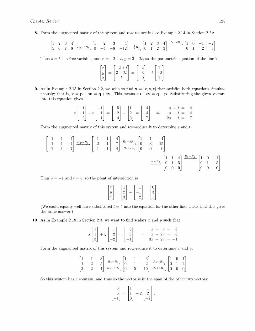
Chapter Review 125
8. Form the augmented matrix of the system and row reduce it (see Example 2.14 in Section 2.2):[1 2 3 45 6 7 8
]R2−5R1−−−−−→
[1 2 3 40 −4 −8 −12
]− 1
4R2−−−−→
[1 2 3 40 1 2 3
]R1−2R2−−−−−→
[1 0 −1 −20 1 2 3
]Thus z = t is a free variable, and x = −2 + t, y = 3− 2t, so the parametric equation of the line isxy
z
=
−2 + t3− 2tt
=
−230
+ t
1−21
.9. As in Example 2.15 in Section 2.2, we wish to find x = [x, y, z] that satisfies both equations simulta-
neously; that is, x = p + su = q + tv. This means su − tv = q − p. Substituting the given vectorsinto this equation gives
s
1−1
2
− t−1
11
=
5−2−4
−1
23
=
4−4−7
⇒s + t = 4−s − t = −42s − t = −7
Form the augmented matrix of this system and row-reduce it to determine s and t:
1 1 4−1 −1 −4
2 −1 −7
R2↔R3−−−−−→
1 1 42 −1 7−1 −1 −4
R2−2R1−−−−−→R3+R1−−−−−→
1 1 40 −3 −150 0 0
− 1
3R2−−−−→
1 1 40 1 50 0 0
R1−R2−−−−−→1 0 −1
0 1 50 0 0
Thus s = −1 and t = 5, so the point of intersection isxy
z
=
123
− 1−1
2
=
031
.(We could equally well have substituted t = 5 into the equation for the other line; check that this givesthe same answer.)
10. As in Example 2.18 in Section 2.3, we want to find scalars x and y such that
x
113
+ y
12−2
=
35−1
⇒x + y = 3x + 2y = 5
3x − 2y = −1
Form the augmented matrix of this system and row-reduce it to determine x and y:1 1 31 2 53 −2 −1
R2−R1−−−−−→R3−3R1−−−−−→
1 1 30 1 20 −5 −10
R1−R2−−−−−→R3+5R3−−−−−→
1 0 10 1 20 0 0
So this system has a solution, and thus so the vector is in the span of the other two vectors: 3
5−1
=
113
+ 2
12−2
.

126 CHAPTER 2. SYSTEMS OF LINEAR EQUATIONS
11. As in Example 2.21 in Section 2.3, the equation of the plane we are looking for isxyz
= s
111
+ t
321
⇒s + 3t = xs + 2t = ys + t = z
Form the augmented matrix and row-reduce it to find conditions for x, y, and z:1 3 x1 2 y1 1 z
R2−R1−−−−−→R3−R2−−−−−→
1 3 x0 −1 y − x0 −2 z − x
−R2−−−→
1 3 x0 1 x− y0 −2 z − x
R3+2R2−−−−−→
1 3 x0 1 x− y0 0 x− 2y + z
We know the system is consistent, since the two given vectors span some plane. So we must havex− 2y + z = 0, and this is the general equation of the plane we were seeking. (An alternative methodwould be to take the cross product of the two given vectors, giving [−1, 2,−1], so that the plane is ofthe form −x+ 2y − z = d; plugging in x = y = z = 0 gives −x+ 2y − z = 0, or x− 2y + z = 0.)
12. As in Example 2.23 in Section 2.3, we want to find scalars c1, c2, and c3 so that
c1
21−3
+ c2
1−1−2
+ c3
39−2
=
000
.Form the augmented matrix of the resulting system and row-reduce it: 2 1 3 0
1 −1 9 0−3 −2 −2 0
−→1 0 4 0
0 1 −5 00 0 0 0
Since c1 = −4c3, c2 = 5c3 is a solution, the vectors are linearly dependent. For example, settingc3 = −1 gives
4
21−3
− 5
1−1−2
− 3
9−2
=
000
.13. By part (a) of Exercise 21 in Section 2.3, it is sufficient to prove that ei is in span(u,v,w) ⊂ R3, since
then we have R3 = span(e1, e2, e3) ⊂ span(u,v,w) ⊂ R3.
(a) Begin with e1. We want to find scalars x, y, and z such that
x
110
+
101
+
011
= e1 =
100
.Form the augmented matrix and row reduce:1 1 0 1
1 0 1 0
0 1 1 0
−→1 0 0 1
2
0 1 0 12
0 0 1 − 12
⇒ e1 =1
2u +
1
2v − 1
2w.
Similarly, for e2,1 1 0 0
1 0 1 1
0 1 1 0
−→1 0 0 1
2
0 1 0 − 12
0 0 1 12
⇒ e1 =1
2u− 1
2v +
1
2w.

Chapter Review 127
Similarly, for e3,1 1 0 0
1 0 1 0
0 1 1 1
−→1 0 0 − 1
2
0 1 0 12
0 0 1 12
⇒ e1 = −1
2u +
1
2v +
1
2w.
Thus R3 = span(u,v,w).
(b) Since w = u + v, these vectors are not linearly independent. But any set of vectors that spansR3 must contain 3 linearly independent vectors, so span(u,v,w) 6= R3.
14. All three statements are true, so (d) is the correct answer. If the vectors are linearly independent, andb is any vector in R3, then the augmented matrix [A |b], when reduced to row echelon form, cannothave a zero row (since otherwise, the portion of the matrix corresponding to A would have a zero row,so the three vectors would be linearly dependent). Thus [A |b] has a unique solution, which can beread off from the row-reduced matrix. This proves statement (c). Next, since there is not a zero row,continuing and putting the system in reduced row-echelon form results in a matrix with 3 leading ones,so it is the identity matrix. Hence the reduced row echelon form of A is I3, and thus A has rank 3.
15. Since A is a 3 × 3 matrix, rank(A) ≤ 3. Since the vectors are linearly dependent, rank(A) cannot be3; since they are not all zero, rank(A) cannot be zero. Thus rank(A) = 1 or rank(A) = 2.
16. By Theorem 2.8 in Section 5.3, the maximum rank of a 5× 3 matrix is 3: since the rows are vectors inR3, any set of four or more of them are linearly dependent. Thus when we row reduce the matrix, wemust introduce at least two zero rows. The minimum rank is zero, achieved when all entries are zero.
17. Suppose that c1(u+v) + c2(u−v) = 0. Rearranging gives (c1 + c2)u+ (c1− c2)v = 0. Since u and vare linearly independent, it follows that c1 + c2 = 0 and c1 − c2 = 0. Adding the two equations gives2c1 = 0, so that c1 = 0; then c2 = 0 as well. It follows that u + v and u− v are linearly independent.
18. Using Exercise 21 in Section 2.3, we show first that u and v are linear combinations of u and u + v.But this is clear: u = u, and v = (u + v) − u. This shows that span(u,v) ⊆ span(u,u + v).Next, we show that u and u + v are linear combinations of u and v. But this is also clear. Thusspan(u,u + v) ⊆ span(u,v). Hence the two spans are equal.
19. Note that rank(A) ≤ rank([A |b]), since any zero rows in an echelon form of [A |b] are also zero rowsin a row echelon form of A, so that a row echelon form of A has at least as many zero rows as a rowechelon form of [A |b]. If rank(A) < rank([A |b]), then a row echelon form of [A |b] will contain at leastone row that is zero in the columns corresponding to A but nonzero in the last column on that row,so that the system will be inconsistent. Hence the system is consistent only if rank(A) = rank([A |b]).
20. Row-reduce both A and B: 1 1 12 3 −1−1 4 1
R2−2R1−−−−−→R3+R1−−−−−→
1 1 10 1 −30 5 2
R3−5R2−−−−−→
1 1 10 1 −30 0 17
1 0 −1
1 1 10 1 3
R2−R1−−−−−→
1 0 −10 1 20 1 3
R3−R2−−−−−→
1 0 −10 1 20 0 1
.Since in row echelon form each of these matrices has no zero rows, it follows that both matrices haverank 3, so that their reduced row echelon forms are both I3. Thus the matrices are row-equivalent.The sequence of row operations required to derive B from A is the sequence of row operations requiredto reduce A to I3, followed by the sequence of row operations, in reverse, required to reduce B to I3.


Chapter 3
Matrices
3.1 Matrix Operations
1. Since A and D have the same shape, this operation makes sense.
A+ 2D =
[3 0−1 5
]+ 2
[0 −3−2 1
]=
[3 0−1 5
]+
[0 −6−4 2
]=
[3 + 0 0− 6−1− 4 5 + 2
]=
[3 −6−5 7
]2. Since D and A have the same shape, this operation makes sense.
3D − 2A = 3
[0 −3−2 1
]− 2
[3 0−1 5
]=
[0 −9−6 3
]−[
6 0−2 10
]=
[0− 6 −9− 0
−6− (−2) 3− 10
]=
[−6 −9−4 −7
]3. Since B is a 2 × 3 matrix and C is a 3 × 2 matrix, they do not have the same shape, so they cannot
be subtracted.
4. Since both C and BT are 3× 2 matrices, this operation makes sense.
C −BT =
1 23 45 6
− [4 −2 10 2 3
]T=
1 23 45 6
− 4 0−2 2
1 3
=
1− 4 2− 03− (−2) 4− 2
5− 1 6− 3
=
−3 25 24 3
5. Since A has two columns and B has two rows, the product makes sense, and
AB =
[3 0−1 5
] [4 −2 10 2 3
]=
[3 · 4 + 0 · 0 3 · (−2) + 0 · 2 3 · 1 + 0 · 3−1 · 4 + 5 · 0 −1 · (−2) + 5 · 2 −1 · 1 + 5 · 3
]=
[12 −6 3−4 12 14
].
6. Since the number of columns of B (3) does not equal the number of rows of D (2), this matrix productdoes not make sense.
7. Since B has three columns and C has three rows, the multiplication BC makes sense, and results in a2 × 2 matrix (since B has 2 rows and C has 2 columns). Since D is also a 2 × 2 matrix, they can besubtracted, so this formula makes sense. First,
BC =
[4 −2 10 2 3
]1 23 45 6
=
[4 · 1− 2 · 3 + 1 · 5 4 · 2− 2 · 4 + 1 · 60 · 1 + 2 · 3 + 3 · 5 0 · 2 + 2 · 4 + 3 · 6
]=
[3 621 26
].
Then
D +BC =
[0 −3−2 1
]+
[3 621 26
]=
[0 + 3 −3 + 6−2 + 21 1 + 26
]=
[3 319 27
].
129
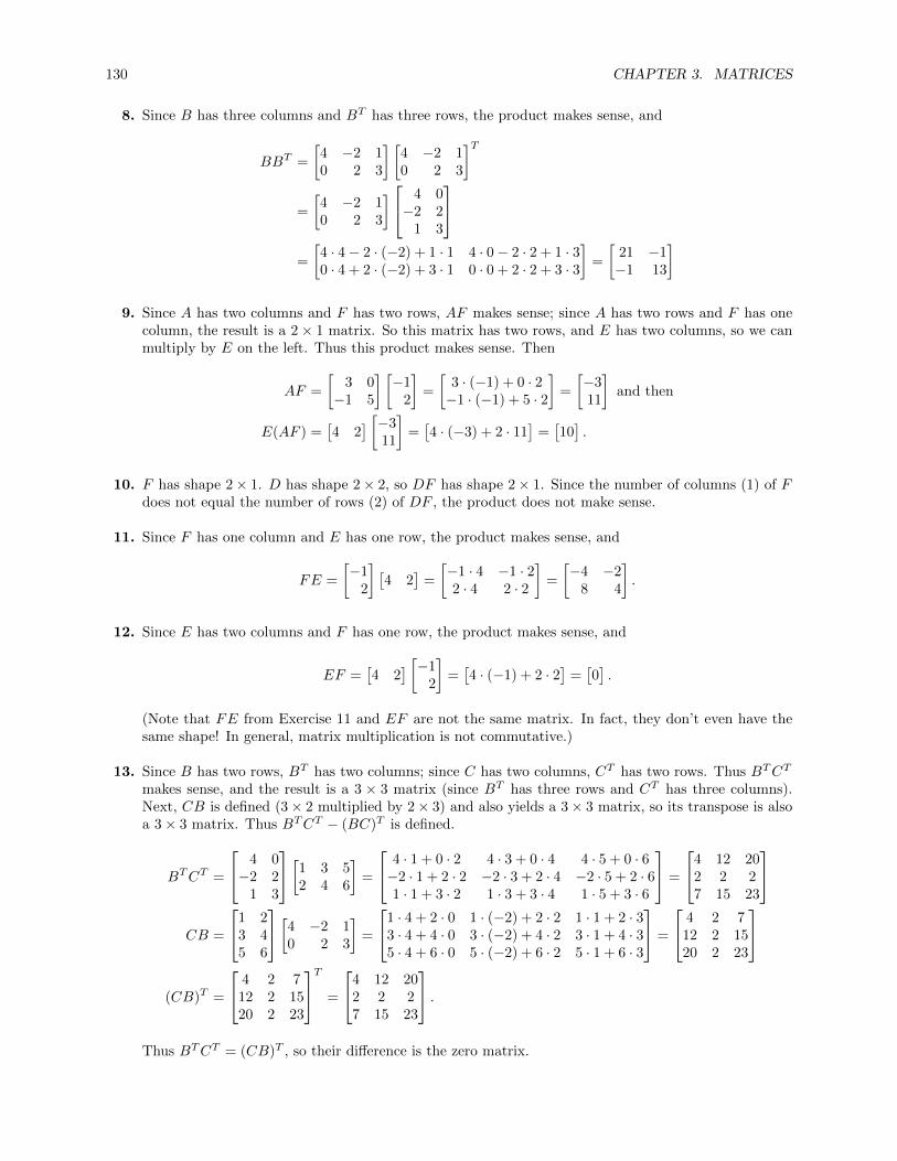
130 CHAPTER 3. MATRICES
8. Since B has three columns and BT has three rows, the product makes sense, and
BBT =
[4 −2 10 2 3
] [4 −2 10 2 3
]T=
[4 −2 10 2 3
] 4 0−2 2
1 3
=
[4 · 4− 2 · (−2) + 1 · 1 4 · 0− 2 · 2 + 1 · 30 · 4 + 2 · (−2) + 3 · 1 0 · 0 + 2 · 2 + 3 · 3
]=
[21 −1−1 13
]
9. Since A has two columns and F has two rows, AF makes sense; since A has two rows and F has onecolumn, the result is a 2× 1 matrix. So this matrix has two rows, and E has two columns, so we canmultiply by E on the left. Thus this product makes sense. Then
AF =
[3 0−1 5
] [−1
2
]=
[3 · (−1) + 0 · 2−1 · (−1) + 5 · 2
]=
[−311
]and then
E(AF ) =[4 2
] [−311
]=[4 · (−3) + 2 · 11
]=[10].
10. F has shape 2× 1. D has shape 2× 2, so DF has shape 2× 1. Since the number of columns (1) of Fdoes not equal the number of rows (2) of DF , the product does not make sense.
11. Since F has one column and E has one row, the product makes sense, and
FE =
[−1
2
] [4 2
]=
[−1 · 4 −1 · 22 · 4 2 · 2
]=
[−4 −2
8 4
].
12. Since E has two columns and F has one row, the product makes sense, and
EF =[4 2
] [−12
]=[4 · (−1) + 2 · 2
]=[0].
(Note that FE from Exercise 11 and EF are not the same matrix. In fact, they don’t even have thesame shape! In general, matrix multiplication is not commutative.)
13. Since B has two rows, BT has two columns; since C has two columns, CT has two rows. Thus BTCT
makes sense, and the result is a 3 × 3 matrix (since BT has three rows and CT has three columns).Next, CB is defined (3× 2 multiplied by 2× 3) and also yields a 3× 3 matrix, so its transpose is alsoa 3× 3 matrix. Thus BTCT − (BC)T is defined.
BTCT =
4 0−2 2
1 3
[1 3 52 4 6
]=
4 · 1 + 0 · 2 4 · 3 + 0 · 4 4 · 5 + 0 · 6−2 · 1 + 2 · 2 −2 · 3 + 2 · 4 −2 · 5 + 2 · 61 · 1 + 3 · 2 1 · 3 + 3 · 4 1 · 5 + 3 · 6
=
4 12 202 2 27 15 23
CB =
1 23 45 6
[4 −2 10 2 3
]=
1 · 4 + 2 · 0 1 · (−2) + 2 · 2 1 · 1 + 2 · 33 · 4 + 4 · 0 3 · (−2) + 4 · 2 3 · 1 + 4 · 35 · 4 + 6 · 0 5 · (−2) + 6 · 2 5 · 1 + 6 · 3
=
4 2 712 2 1520 2 23
(CB)T =
4 2 712 2 1520 2 23
T =
4 12 202 2 27 15 23
.Thus BTCT = (CB)T , so their difference is the zero matrix.

3.1. MATRIX OPERATIONS 131
14. Since A and D are both 2× 2 matrices, the products in both orders are defined, and each results in a2× 2 matrix, so their difference is defined as well.
DA =
[0 −3−2 1
] [3 0−1 5
]=
[0 · 3− 3 · (−1) 0 · 0− 3 · 5−2 · 3 + 1 · (−1) −2 · 0 + 1 · 5
]=
[3 −15−7 5
]AD =
[3 0−1 5
] [0 −3−2 1
]=
[3 · 0 + 0 · (−2) 3 · (−3) + 0 · 1−1 · 0 + 5 · (−2) −1 · (−3) + 5 · 1
]=
[0 −9
−10 8
]DA−AD =
[3 −15−7 5
]−[
0 −9−10 8
]=
[3− 0 −15− (−9)
−7− (−10) 5− 8
]=
[3 −63 −3
].
15. Since A is 2× 2, A2 is defined and is also a 2× 2 matrix, so we can multiply by A again to get A3.
A2 =
[3 0−1 5
] [3 0−1 5
]=
[3 · 3 + 0 · (−1) 3 · 0 + 0 · 5−1 · 3 + 5 · (−1) −1 · 0 + 5 · 5
]=
[9 0−8 25
]A3 = AA2 =
[3 0−1 5
] [9 0−8 25
]=
[3 · 9 + 0 · (−8) 3 · 0 + 0 · 25−1 · 9 + 5 · (−8) −1 · 0 + 5 · 25
]=
[27 0−49 125
].
16. Since D is a 2× 2 matrix, I2−A makes sense and is also a 2× 2 matrix. Since it has the same numberof rows as columns, squaring it (which is multiplying it by itself) also makes sense.
I2 −D =
[1 00 1
]−[
0 −3−2 1
]=
[1 32 0
].
Thus
(I2 −D)2 =
[1 32 0
]2
=
[1 · 1 + 3 · 2 1 · 3 + 3 · 02 · 1 + 0 · 2 2 · 3 + 0 · 0
]=
[7 32 6
]
17. Suppose that A =
[a bc d
]. Then if A2 = 0,
A2 =
[a bc d
] [a bc d
]=
[a2 + bc ab+ bdac+ cd bc+ d2
]=
[0 00 0
]If c = 0, so that the upper right-hand entry is zero, then we must also have a = 0 and d = 0 so that
the diagonal entries are zero. So
[0 01 0
]is one solution. Alternatively, if c 6= 0, then ac = −cd and
thus a = −d. This will make the lower left entry zero as well, and the two diagonal entries will bothbe equal to a2 + bc. So any values of a, b, and c 6= 0 with a2 = −bc will work. For example, a = b = 1,c = −1, d = −1: [
1 1−1 −1
] [1 1−1 −1
]=
[1− 1 1− 1−1 + 1 −1 + 1
]=
[0 00 0
].
18. Note that the first column of A is twice its second column. Thus
A
[1 0−2 0
]=
[0 00 0
]= A
[0 00 0
].
19. The cost of shipping one unit of each product is given by B =
[1.50 1.00 2.001.75 1.50 1.00
], where the first row
gives the costs of shipping each product by truck, and the second row the costs when shipping by train.Then BA gives the costs of shipping all the products to each of the warehouses by truck or train:
BA =
[1.50 1.00 2.001.75 1.50 1.00
]200 75150 100100 125
=
[650.00 462.50675.00 406.25
].
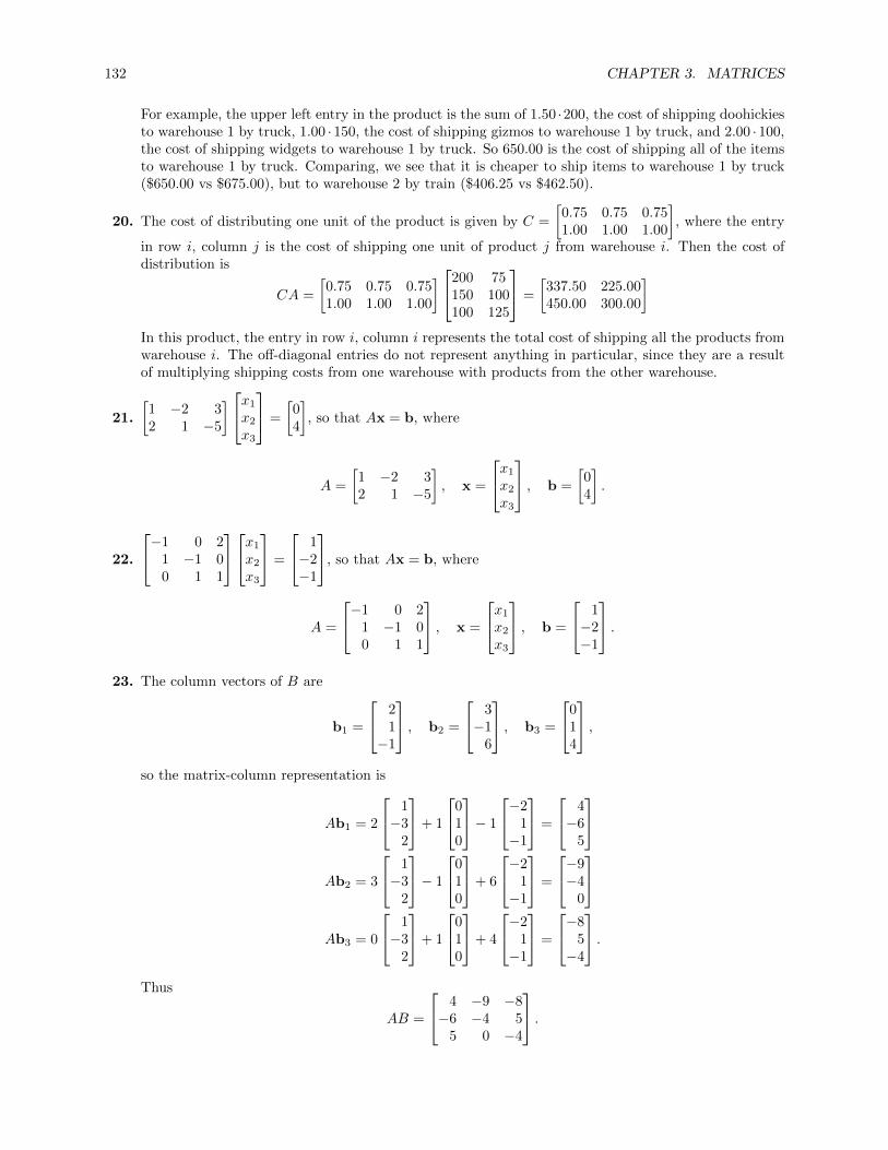
132 CHAPTER 3. MATRICES
For example, the upper left entry in the product is the sum of 1.50 ·200, the cost of shipping doohickiesto warehouse 1 by truck, 1.00 · 150, the cost of shipping gizmos to warehouse 1 by truck, and 2.00 · 100,the cost of shipping widgets to warehouse 1 by truck. So 650.00 is the cost of shipping all of the itemsto warehouse 1 by truck. Comparing, we see that it is cheaper to ship items to warehouse 1 by truck($650.00 vs $675.00), but to warehouse 2 by train ($406.25 vs $462.50).
20. The cost of distributing one unit of the product is given by C =
[0.75 0.75 0.751.00 1.00 1.00
], where the entry
in row i, column j is the cost of shipping one unit of product j from warehouse i. Then the cost ofdistribution is
CA =
[0.75 0.75 0.751.00 1.00 1.00
]200 75150 100100 125
=
[337.50 225.00450.00 300.00
]In this product, the entry in row i, column i represents the total cost of shipping all the products fromwarehouse i. The off-diagonal entries do not represent anything in particular, since they are a resultof multiplying shipping costs from one warehouse with products from the other warehouse.
21.
[1 −2 32 1 −5
]x1
x2
x3
=
[04
], so that Ax = b, where
A =
[1 −2 32 1 −5
], x =
x1
x2
x3
, b =
[04
].
22.
−1 0 21 −1 00 1 1
x1
x2
x3
=
1−2−1
, so that Ax = b, where
A =
−1 0 21 −1 00 1 1
, x =
x1
x2
x3
, b =
1−2−1
.23. The column vectors of B are
b1 =
21−1
, b2 =
3−1
6
, b3 =
014
,so the matrix-column representation is
Ab1 = 2
1−3
2
+ 1
010
− 1
−21−1
=
4−6
5
Ab2 = 3
1−3
2
− 1
010
+ 6
−21−1
=
−9−4
0
Ab3 = 0
1−3
2
+ 1
010
+ 4
−21−1
=
−85−4
.Thus
AB =
4 −9 −8−6 −4 5
5 0 −4
.

3.1. MATRIX OPERATIONS 133
24. The row vectors of A are
A1 =[1 0 −2
], A2 =
[−3 1 1
], A3 =
[2 0 −1
],
so the row-matrix representation is
A1B = 1[2 3 0
]+ 0
[1 −1 1
]− 2
[−1 6 4
]=[4 −9 −8
]A2B = −3
[2 3 0
]+ 1
[1 −1 1
]+ 1
[−1 6 4
]=[−6 −4 5
]A3B = 2
[2 3 0
]+ 0
[1 −1 1
]− 1
[−1 6 4
]=[5 0 −4
].
Thus
AB =
4 −9 −8−6 −4 5
5 0 −4
.25. The outer product expansion is
a1B1 + a2B2 + a3B3 =
1−3
2
[2 3 0]
+
010
[1 −1 1]
+
−21−1
[−1 6 4]
=
2 3 0−6 −9 0
4 6 0
+
0 0 01 −1 10 0 0
+
2 −12 −8−1 6 4
1 −6 −4
=
4 −9 −8−6 −4 5
5 0 −4
.26. We have
Ba1 = 1
21−1
− 3
3−1
6
+ 2
014
=
−76
−11
Ba2 = 0
21−1
+ 1
3−1
6
+ 0
014
=
3−1
6
Ba3 = −2
21−1
+ 1
3−1
6
− 1
014
=
−1−4
4
.Thus
BA =
−7 3 −16 −1 −4
−11 6 4
.27. We have
B1A = 2[1 0 −2
]+ 3
[−3 1 1
]+ 0
[2 0 −1
]=[−7 3 −1
]B2A = 1
[1 0 −2
]− 1
[−3 1 1
]+ 1
[2 0 −1
]=[6 −1 −4
]B3A = −1
[1 0 −2
]+ 6
[−3 1 1
]+ 4
[2 0 −1
]=[−11 6 4
].
Thus
BA =
−7 3 −16 −1 −4
−11 6 4
.
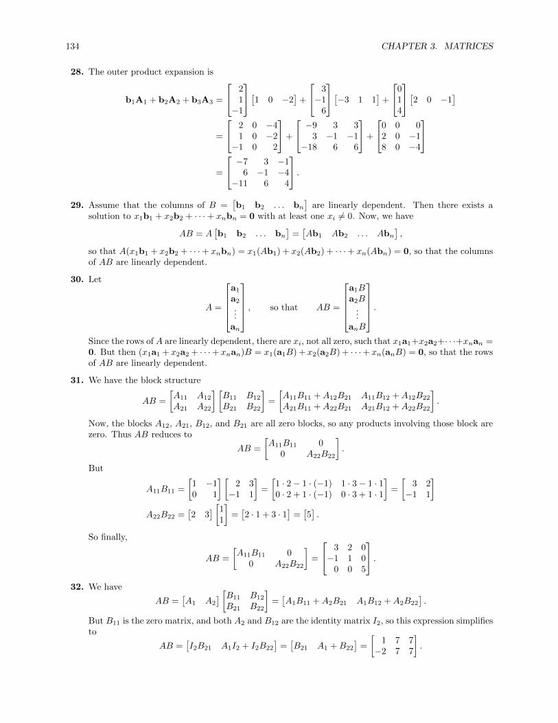
134 CHAPTER 3. MATRICES
28. The outer product expansion is
b1A1 + b2A2 + b3A3 =
21−1
[1 0 −2]
+
3−1
6
[−3 1 1]
+
014
[2 0 −1]
=
2 0 −41 0 −2−1 0 2
+
−9 3 33 −1 −1
−18 6 6
+
0 0 02 0 −18 0 −4
=
−7 3 −16 −1 −4
−11 6 4
.29. Assume that the columns of B =
[b1 b2 . . . bn
]are linearly dependent. Then there exists a
solution to x1b1 + x2b2 + · · ·+ xnbn = 0 with at least one xi 6= 0. Now, we have
AB = A[b1 b2 . . . bn
]=[Ab1 Ab2 . . . Abn
],
so that A(x1b1 + x2b2 + · · ·+ xnbn) = x1(Ab1) + x2(Ab2) + · · ·+ xn(Abn) = 0, so that the columnsof AB are linearly dependent.
30. Let
A =
a1
a2
...an
, so that AB =
a1Ba2B
...anB
.Since the rows of A are linearly dependent, there are xi, not all zero, such that x1a1+x2a2+· · ·+xnan =0. But then (x1a1 + x2a2 + · · ·+ xnan)B = x1(a1B) + x2(a2B) + · · ·+ xn(anB) = 0, so that the rowsof AB are linearly dependent.
31. We have the block structure
AB =
[A11 A12
A21 A22
] [B11 B12
B21 B22
]=
[A11B11 +A12B21 A11B12 +A12B22
A21B11 +A22B21 A21B12 +A22B22
].
Now, the blocks A12, A21, B12, and B21 are all zero blocks, so any products involving those block arezero. Thus AB reduces to
AB =
[A11B11 0
0 A22B22
].
But
A11B11 =
[1 −10 1
] [2 3−1 1
]=
[1 · 2− 1 · (−1) 1 · 3− 1 · 10 · 2 + 1 · (−1) 0 · 3 + 1 · 1
]=
[3 2−1 1
]A22B22 =
[2 3
] [11
]=[2 · 1 + 3 · 1
]=[5].
So finally,
AB =
[A11B11 0
0 A22B22
]=
3 2 0−1 1 0
0 0 5
.32. We have
AB =[A1 A2
] [B11 B12
B21 B22
]=[A1B11 +A2B21 A1B12 +A2B22
].
But B11 is the zero matrix, and both A2 and B12 are the identity matrix I2, so this expression simplifiesto
AB =[I2B21 A1I2 + I2B22
]=[B21 A1 +B22
]=
[1 7 7−2 7 7
].

3.1. MATRIX OPERATIONS 135
33. We have the block structure
AB =
[A11 A12
A21 A22
] [B11 B12
B21 B22
]=
[A11B11 +A12B21 A11B12 +A12B22
A21B11 +A22B21 A21B12 +A22B22
].
Now, B21 is the zero matrix, so products involving that block are zero. Further, A12, A21, and B11 areall the identity matrix I2. So this product simplifies to
AB =
[A11I2 A11B12 + I2B22
I2I2 I2B12 +A22B22
]=
[A11 A11B12 +B22
I2 B12 +A22B22
].
The remaining products are
A11B12 +B22 =
[1 23 4
] [0 11 0
]+B22 =
[2 14 3
]+
[0 −11 0
]=
[2 05 3
]B12 +A22B22 = B12 +
[−1 1
1 −1
] [0 −11 0
]=
[0 11 0
]+
[1 1−1 −1
]=
[1 20 −1
].
Thus
AB =
1 2 2 03 4 5 31 0 1 20 1 0 −1
.34. We have the block structure
AB =
[A11 A12
A21 A22
] [B11 B12
B21 B22
]=
[A11B11 +A12B21 A11B12 +A12B22
A21B11 +A22B21 A21B12 +A22B22
].
Now, A11 is the identity matrix I3, and A21 is the zero matrix. Further, B22 is a 1 × 1 matrix, as isA22, so they both behave just like scalar multiplication. Thus this product reduces to
AB =
[I3B11 +A12B21 I3B12 −A12
4B21 4 · (−1)
]=
[B11 +A12B21 B12 −A12
4B21 −4
].
Compute the matrices in the first row:
B11 +A12B21 = B11 +
123
[1 1 1]
=
1 2 30 1 40 0 1
+
1 1 12 2 23 3 3
=
2 3 42 3 63 3 4
B12 −A12 =
111
−1
23
=
0−1−2
.So
AB =
2 3 4 02 3 6 −13 3 4 −24 4 4 −4
.35. (a) Computing the powers of A as required, we get
A2 =
[−1 1−1 0
], A3 =
[−1 0
0 −1
], A4 =
[0 −11 −1
],
A5 =
[1 −11 0
], A6 =
[1 00 1
]= I2, A7 =
[0 1−1 1
]= A.
Note that A6 = I2 and A7 = A.
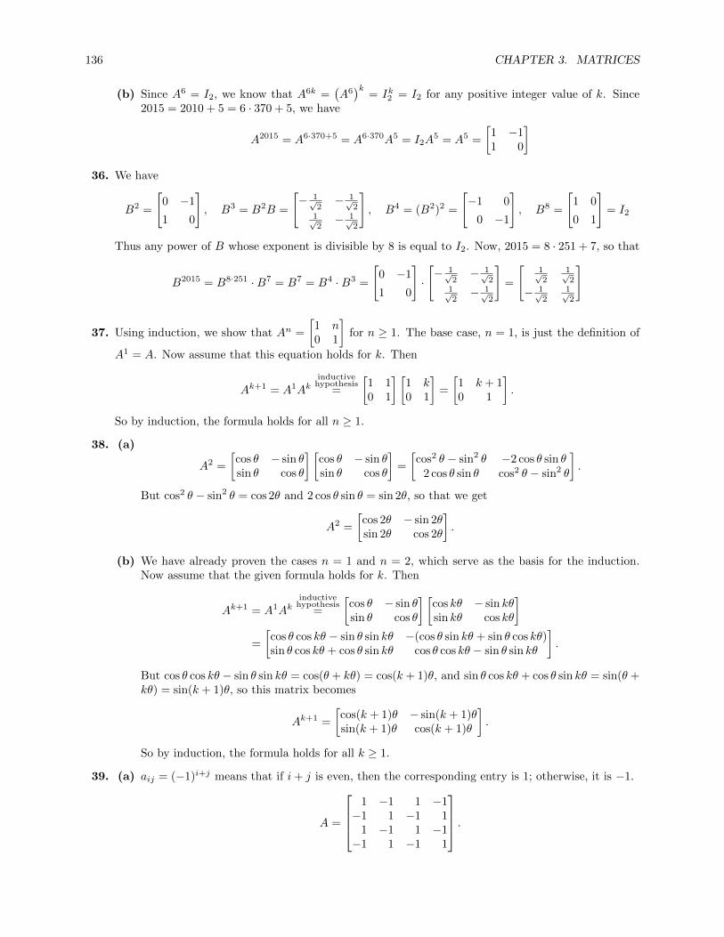
136 CHAPTER 3. MATRICES
(b) Since A6 = I2, we know that A6k =(A6)k
= Ik2 = I2 for any positive integer value of k. Since2015 = 2010 + 5 = 6 · 370 + 5, we have
A2015 = A6·370+5 = A6·370A5 = I2A5 = A5 =
[1 −11 0
]36. We have
B2 =
[0 −1
1 0
], B3 = B2B =
[− 1√
2− 1√
21√2− 1√
2
], B4 = (B2)2 =
[−1 0
0 −1
], B8 =
[1 0
0 1
]= I2
Thus any power of B whose exponent is divisible by 8 is equal to I2. Now, 2015 = 8 · 251 + 7, so that
B2015 = B8·251 ·B7 = B7 = B4 ·B3 =
[0 −1
1 0
]·
[− 1√
2− 1√
21√2− 1√
2
]=
[1√2
1√2
− 1√2
1√2
]
37. Using induction, we show that An =
[1 n0 1
]for n ≥ 1. The base case, n = 1, is just the definition of
A1 = A. Now assume that this equation holds for k. Then
Ak+1 = A1Akinductive
hypothesis=
[1 10 1
] [1 k0 1
]=
[1 k + 10 1
].
So by induction, the formula holds for all n ≥ 1.
38. (a)
A2 =
[cos θ − sin θsin θ cos θ
] [cos θ − sin θsin θ cos θ
]=
[cos2 θ − sin2 θ −2 cos θ sin θ
2 cos θ sin θ cos2 θ − sin2 θ
].
But cos2 θ − sin2 θ = cos 2θ and 2 cos θ sin θ = sin 2θ, so that we get
A2 =
[cos 2θ − sin 2θsin 2θ cos 2θ
].
(b) We have already proven the cases n = 1 and n = 2, which serve as the basis for the induction.Now assume that the given formula holds for k. Then
Ak+1 = A1Akinductive
hypothesis=
[cos θ − sin θsin θ cos θ
] [cos kθ − sin kθsin kθ cos kθ
]=
[cos θ cos kθ − sin θ sin kθ −(cos θ sin kθ + sin θ cos kθ)sin θ cos kθ + cos θ sin kθ cos θ cos kθ − sin θ sin kθ
].
But cos θ cos kθ − sin θ sin kθ = cos(θ + kθ) = cos(k + 1)θ, and sin θ cos kθ + cos θ sin kθ = sin(θ +kθ) = sin(k + 1)θ, so this matrix becomes
Ak+1 =
[cos(k + 1)θ − sin(k + 1)θsin(k + 1)θ cos(k + 1)θ
].
So by induction, the formula holds for all k ≥ 1.
39. (a) aij = (−1)i+j means that if i+ j is even, then the corresponding entry is 1; otherwise, it is −1.
A =
1 −1 1 −1−1 1 −1 1
1 −1 1 −1−1 1 −1 1
.

3.1. MATRIX OPERATIONS 137
(b) Each entry is its row number minus its column number:
A =
0 −1 −2 −31 0 −1 −22 1 0 −13 2 1 0
.(c)
A =
(1− 1)1 (1− 1)2 (1− 1)3 (1− 1)4
(2− 1)1 (2− 1)2 (2− 1)3 (2− 1)4
(3− 1)1 (3− 1)2 (3− 1)3 (3− 1)4
(4− 1)1 (4− 1)2 (4− 1)3 (4− 1)4
=
0 0 0 01 1 1 12 4 8 163 9 27 81
.(d)
A =
sin (1+1−1)π
4 sin (1+2−1)π4 sin (1+3−1)π
4 sin (1+4−1)π4
sin (2+1−1)π4 sin (2+2−1)π
4 sin (2+3−1)π4 sin (2+4−1)π
4
sin (3+1−1)π4 sin (3+2−1)π
4 sin (3+3−1)π4 sin (3+4−1)π
4
sin (4+1−1)π4 sin (4+2−1)π
4 sin (4+3−1)π4 sin (4+4−1)π
4
=
sin π
4 sin π2 sin 3π
4 sinπ
sin π2 sin 3π
4 sinπ sin 5π4
sin 3π4 sinπ sin 5π
4 sin 3π2
sinπ sin 5π4 sin 3π
2 sin 7π4
=
√
22 1
√2
2 0
1√
22 0 −
√2
2√2
2 0 −√
22 −1
0 −√
22 −1 −
√2
2
.40. (a) This matrix has zeros whenever the row number exceeds the column number, and the nonzero
entries are the sum of the row and column numbers:
A =
2 3 4 5 6 70 4 5 6 7 80 0 6 7 8 90 0 0 8 9 100 0 0 0 10 110 0 0 0 0 12
.
(b) This matrix has 1’s on the main diagonal and one diagonal away from the main diagonal, andzeros elsewhere:
A =
1 1 0 0 0 01 1 1 0 0 00 1 1 1 0 00 0 1 1 1 00 0 0 1 1 10 0 0 0 1 1
.(c) This matrix is zero except where the row number plus the column number is 6, 7, or 8:
A =
0 0 0 0 1 10 0 0 1 1 10 0 1 1 1 00 1 1 1 0 01 1 1 0 0 01 1 0 0 0 0
.
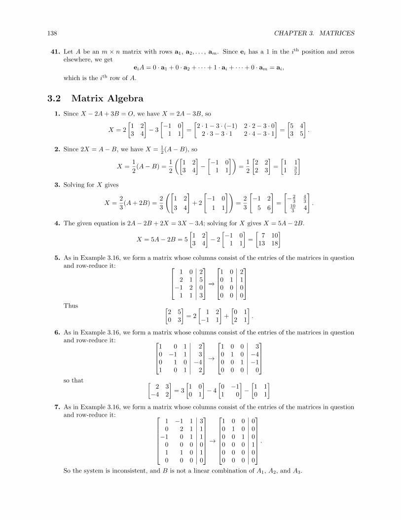
138 CHAPTER 3. MATRICES
41. Let A be an m × n matrix with rows a1, a2, . . . , am. Since ei has a 1 in the ith position and zeroselsewhere, we get
eiA = 0 · a1 + 0 · a2 + · · ·+ 1 · ai + · · ·+ 0 · am = ai,
which is the ith row of A.
3.2 Matrix Algebra
1. Since X − 2A+ 3B = O, we have X = 2A− 3B, so
X = 2
[1 23 4
]− 3
[−1 0
1 1
]=
[2 · 1− 3 · (−1) 2 · 2− 3 · 0
2 · 3− 3 · 1 2 · 4− 3 · 1
]=
[5 43 5
].
2. Since 2X = A−B, we have X = 12 (A−B), so
X =1
2(A−B) =
1
2
([1 23 4
]−[−1 0
1 1
])=
1
2
[2 22 3
]=
[1 11 3
2
]3. Solving for X gives
X =2
3(A+ 2B) =
2
3
([1 2
3 4
]+ 2
[−1 0
1 1
])=
2
3
[−1 2
5 6
]=
[− 2
343
103 4
].
4. The given equation is 2A− 2B + 2X = 3X − 3A; solving for X gives X = 5A− 2B.
X = 5A− 2B = 5
[1 23 4
]− 2
[−1 0
1 1
]=
[7 10
13 18
]5. As in Example 3.16, we form a matrix whose columns consist of the entries of the matrices in question
and row-reduce it: 1 0 22 1 5−1 2 0
1 1 3
−→
1 0 20 1 10 0 00 0 0
Thus [
2 50 3
]= 2
[1 2−1 1
]+
[0 12 1
].
6. As in Example 3.16, we form a matrix whose columns consist of the entries of the matrices in questionand row-reduce it:
1 0 1 20 −1 1 30 1 0 −41 0 1 2
→
1 0 0 30 1 0 −40 0 1 −10 0 0 0
so that [
2 3−4 2
]= 3
[1 00 1
]− 4
[0 −11 0
]−[1 10 1
]7. As in Example 3.16, we form a matrix whose columns consist of the entries of the matrices in question
and row-reduce it: 1 −1 1 30 2 1 1−1 0 1 1
0 0 0 01 1 0 10 0 0 0
→
1 0 0 00 1 0 00 0 1 00 0 0 10 0 0 00 0 0 0
.So the system is inconsistent, and B is not a linear combination of A1, A2, and A3.
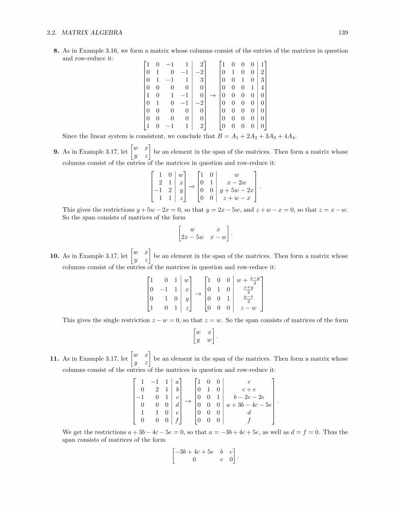
3.2. MATRIX ALGEBRA 139
8. As in Example 3.16, we form a matrix whose columns consist of the entries of the matrices in questionand row-reduce it:
1 0 −1 1 20 1 0 −1 −20 1 −1 1 30 0 0 0 01 0 1 −1 00 1 0 −1 −20 0 0 0 00 0 0 0 01 0 −1 1 2
→
1 0 0 0 10 1 0 0 20 0 1 0 30 0 0 1 40 0 0 0 00 0 0 0 00 0 0 0 00 0 0 0 00 0 0 0 0
Since the linear system is consistent, we conclude that B = A1 + 2A2 + 3A3 + 4A4.
9. As in Example 3.17, let
[w xy z
]be an element in the span of the matrices. Then form a matrix whose
columns consist of the entries of the matrices in question and row-reduce it:1 0 w2 1 x−1 2 y
1 1 z
−→
1 0 w0 1 x− 2w0 0 y + 5w − 2x0 0 z + w − x
.This gives the restrictions y+ 5w− 2x = 0, so that y = 2x− 5w, and z+w−x = 0, so that z = x−w.So the span consists of matrices of the form[
w x2x− 5w x− w
].
10. As in Example 3.17, let
[w xy z
]be an element in the span of the matrices. Then form a matrix whose
columns consist of the entries of the matrices in question and row-reduce it:1 0 1 w
0 −1 1 x
0 1 0 y
1 0 1 z
→
1 0 0 w + x−y2
0 1 0 x+y2
0 0 1 y−x2
0 0 0 z − w
This gives the single restriction z−w = 0, so that z = w. So the span consists of matrices of the form[
w xy w
].
11. As in Example 3.17, let
[w xy z
]be an element in the span of the matrices. Then form a matrix whose
columns consist of the entries of the matrices in question and row-reduce it:1 −1 1 a0 2 1 b−1 0 1 c
0 0 0 d1 1 0 e0 0 0 f
→
1 0 0 e0 1 0 c+ e0 0 1 b− 2c− 2e0 0 0 a+ 3b− 4c− 5e0 0 0 d0 0 0 f
.
We get the restrictions a+ 3b− 4c− 5e = 0, so that a = −3b+ 4c+ 5e, as well as d = f = 0. Thus thespan consists of matrices of the form [
−3b+ 4c+ 5e b c0 e 0
].

140 CHAPTER 3. MATRICES
12. As in Example 3.17, let
x1 x2 x3
x4 x5 x6
x7 x8 x9
be an element in the span of the matrices. Then form a matrix
whose columns consist of the entries of the matrices in question and row-reduce it:
1 0 −1 1 x1
0 1 0 −1 x2
0 1 −1 1 x3
0 0 0 0 x4
1 0 1 −1 x5
0 1 0 −1 x6
0 0 0 0 x7
0 0 0 0 x8
1 0 −1 1 x9
→
1 0 0 0 x1+x5
2
0 1 0 0 x3 + x5−x1
2
0 0 1 0 x3 + x5 − x1 − x2
0 0 0 1 x3 − x2 + x5−x1
2
0 0 0 0 x6 − x2
0 0 0 0 x4
0 0 0 0 x7
0 0 0 0 x8
0 0 0 0 x9 − x1
We get the restrictions
x6 = x2, x9 = x1, x4 = x7 = x8 = 0.
Thus the span consists of matrices of the formx1 x2 x3
0 x5 x6
0 0 x1
.13. Following Example 3.18, we construct an augmented matrix whose columns are the entries of the given
matrices and with zeros in the constant column, and row-reduce it:1 4 02 3 03 2 04 1 0
→
1 0 00 1 00 0 00 0 0
Since the only solution is the trivial solution, we conclude that these matrices are linearly independent.
14. Following Example 3.18, we construct an augmented matrix whose columns are the entries of the givenmatrices and with zeros in the constant column, and row-reduce it:
1 2 1 0
2 1 1 0
4 −1 1 0
3 0 1 0
→
1 0 13 0
0 1 13 0
0 0 0 0
0 0 0 0
Since the system has a nontrivial solution, the original matrices are not linearly independent; in fact,from the solutions we get from the row-reduced matrix,
1
3
[1 24 3
]+
1
3
[2 1−1 0
]=
[1 11 1
]15. Following Example 3.18, we construct an augmented matrix whose columns are the entries of the given
matrices and with zeros in the constant column, and row-reduce it:0 1 −2 −1 01 0 −1 −3 05 2 0 1 02 3 1 9 0−1 1 0 4 0
0 1 2 5 0
→
1 0 0 0 00 1 0 0 00 0 1 0 00 0 0 1 00 0 0 0 00 0 0 0 0
Since the only solution is the trivial solution, we conclude that these matrices are linearly independent.

3.2. MATRIX ALGEBRA 141
16. Following Example 3.18, we construct an augmented matrix whose columns are the entries of the givenmatrices and with zeros in the constant column, and row-reduce it:
1 2 1 −1 0−1 1 2 1 0
0 0 0 0 00 0 0 0 02 3 1 −1 00 0 0 0 00 0 0 0 02 4 3 0 06 9 5 −4 0
→
1 0 0 0 00 1 0 0 00 0 1 0 00 0 0 1 00 0 0 0 00 0 0 0 00 0 0 0 00 0 0 0 00 0 0 0 0
The only solution is the trivial solution, so the matrices are linearly independent.
17. Let A, B, and C be m× n matrices.
(a)
A+B =
a11 . . . a1n
.... . .
...am1 . . . amn
+
b11 . . . b1n...
. . ....
bm1 . . . bmn
=
a11 + b11 . . . a1n + b1n...
. . ....
am1 + bm1 . . . amn + bmn
=
b11 + a11 . . . b1n + a1n
.... . .
...bm1 + am1 . . . bmn + amn
=
b11 . . . b1n...
. . ....
bm1 . . . bmn
+
a11 . . . a1n
.... . .
...am1 . . . amn
= B +A.
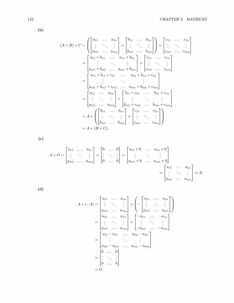
142 CHAPTER 3. MATRICES
(b)
(A+B) + C =
a11 . . . a1n
.... . .
...am1 . . . amn
+
b11 . . . b1n...
. . ....
bm1 . . . bmn
+
c11 . . . c1n...
. . ....
cm1 . . . cmn
=
a11 + b11 . . . a1n + b1n...
. . ....
am1 + bm1 . . . amn + bmn
+
c11 . . . c1n...
. . ....
cm1 . . . cmn
=
a11 + b11 + c11 . . . a1n + b1n + c1n...
. . ....
am1 + bm1 + cm1 . . . amn + bmn + cmn
=
a11 . . . a1n
.... . .
...am1 . . . amn
+
b11 + c11 . . . b1n + c1n...
. . ....
bm1 + cm1 . . . bmn + cmn
= A+
b11 . . . b1n
.... . .
...bm1 . . . bmn
+
c11 . . . c1n...
. . ....
cm1 . . . cmn
= A+ (B + C).
(c)
A+O =
a11 . . . a1n
.... . .
...am1 . . . amn
+
0 . . . 0...
. . ....
0 . . . 0
=
a11 + 0 . . . a1n + 0...
. . ....
am1 + 0 . . . amn + 0
=
a11 . . . a1n
.... . .
...am1 . . . amn
= A.
(d)
A+ (−A) =
a11 . . . a1n
.... . .
...am1 . . . amn
+
−a11 . . . a1n
.... . .
...am1 . . . amn
=
a11 . . . a1n
.... . .
...am1 . . . amn
+
−a11 . . . −a1n
.... . .
...−am1 . . . −amn
=
a11 − a11 . . . a1n − a1n
.... . .
...am1 − am1 . . . amn − amn
=
0 . . . 0...
. . ....
0 . . . 0
= O.

3.2. MATRIX ALGEBRA 143
18. Let A and B be m× n matrices, and c and d be scalars.
(a)
c(A+B) = c
a11 . . . a1n
.... . .
...am1 . . . amn
+
b11 . . . b1n...
. . ....
bm1 . . . bmn
= c
a11 + b11 . . . a1n + b1n
.... . .
...am1 + bm1 . . . amn + bmn
=
c(a11 + b11) . . . c(a1n + b1n)...
. . ....
c(am1 + bm1) . . . c(amn + bmn)
=
ca11 + cb11 . . . ca1n + cb1n...
. . ....
cam1 + cbm1 . . . camn + cbmn
=
ca11 . . . ca1n
.... . .
...cam1 . . . camn
+
cb11 . . . cb1n...
. . ....
cbm1 . . . cbmn
= c
a11 . . . a1n
.... . .
...am1 . . . amn
+ c
b11 . . . b1n...
. . ....
bm1 . . . bmn
= cA+ cB.
(b)
(c+ d)A = (c+ d)
a11 . . . a1n
.... . .
...am1 . . . amn
=
(c+ d)a11 . . . (c+ d)a1n
.... . .
...(c+ d)am1 . . . (c+ d)amn
=
ca11 + da11 . . . ca1n + d1n
.... . .
...cam1 + dam1 . . . camn + damn
=
ca11 . . . ca1n
.... . .
...cam1 . . . camn
+
da11 . . . da1n
.... . .
...dam1 . . . damn
= c
a11 . . . a1n
.... . .
...am1 . . . amn
+ d
a11 . . . a1n
.... . .
...am1 . . . amn
= cA+ dA.

144 CHAPTER 3. MATRICES
(c)
c(dA) = c
da11 . . . da1n
.... . .
...dam1 . . . damn
=
cda11 . . . cda1n
.... . .
...cdam1 . . . cdamn
= cd
a11 . . . a1n
.... . .
...am1 . . . amn
.(d)
1A = 1
a11 . . . a1n
.... . .
...am1 . . . amn
=
1a11 . . . 1a1n
.... . .
...1am1 . . . 1amn
=
a11 . . . a1n
.... . .
...am1 . . . amn
= A.
19. Let A and B be r × n matrices, and C be an n× s matrix, so that the product makes sense. Then
(A+B)C =
a11 . . . a1n
.... . .
...ar1 . . . arn
+
b11 . . . b1n...
. . ....
br1 . . . brn
c11 . . . c1s
.... . .
...cn1 . . . cns
=
a11 + b11 . . . a1n + b1n...
. . ....
ar1 + br1 . . . arn + brn
c11 . . . c1s
.... . .
...cn1 . . . cns
=
(a11 + b11)c11 + · · ·+ (a1n + b1n)cn1 . . . (a11 + b11)c1s + · · ·+ (a1n + b1n)cns...
. . ....
(ar1 + br1)c11 + · · ·+ (arn + brn)cn1 . . . (ar1 + br1)c1s + · · ·+ (ar1 + br1)c1s
=
a11c11 + · · ·+ a1ncn1 . . . a11c1s + · · ·+ a1ncns...
. . ....
ar1c11 + · · ·+ arncn1 . . . ar1c1s + · · ·+ ar1cns
+
b11c11 + · · ·+ b1ncn1 . . . b11c1s + · · ·+ b1ncns...
. . ....
br1c11 + · · ·+ brncn1 . . . br1c1s + · · ·+ br1cns
= AC +BC.
20. Let A be an r × n matrix and C be an n × s matrix, so that the product makes sense. Let k be ascalar. Then
k(AB) = k
a11c11 + · · ·+ a1ncn1 · · · a11c1s + · · ·+ a1ncns
.... . .
...ar1c11 + · · ·+ arncn1 · · · ar1c1s + · · ·+ arncns
=
k(a11c11 + · · ·+ a1ncn1) · · · k(a11c1s + · · ·+ a1ncns)...
. . ....
k(ar1c11 + · · ·+ arncn1) · · · k(ar1c1s + · · ·+ arncns)
=
(ka11)c11 + · · ·+ (ka1n)cn1 · · · (ka11)c1s + · · ·+ (ka1n)cns...
. . ....
(kar1)c11 + · · ·+ (karn)cn1 · · · (kar1)c1s + · · ·+ (karn)cns
=
ka11 . . . ka1n
.... . .
...kar1 . . . karn
c11 . . . c1s
.... . .
...cn1 . . . cns
= (kA)B.

3.2. MATRIX ALGEBRA 145
That proves the first equality. Regrouping the expression on the second line above differently, we get
k(AB) =
a11(kc11) + · · ·+ a1n(kcn1) · · · a11(kc1s) + · · ·+ a1n(kcns)...
. . ....
ar1(kc11) + · · ·+ arn(kcn1) · · · ar1(kc1s) + · · ·+ arn(kcns)
=
a11 . . . a1n
.... . .
...ar1 . . . arn
kc11 . . . kc1s
.... . .
...kcn1 . . . kcns
= A(kB).
21. If A is m× n, then to prove ImA = A, note that
Im =
e1
e2
...em
,where ei is a standard (row) unit vector; then
ImA =
e1
e2
...em
A =
e1Ae2A
...emA
=
A1
A2
...Am
= A.
22. Note that
(A−B)(A+B) = A(A+B)−B(A+B) = A2 +AB −BA+B2 = (A2 +B2) + (AB −BA),
so that (A−B)(A+B) = A2 +B2 if and only if AB −BA = O; that is, if and only if AB = BA.
23. Compute both AB and BA:
AB =
[1 10 1
] [a bc d
]=
[a+ c b+ dc d
]BA =
[a bc d
] [1 10 1
]=
[a a+ bc c+ d
].
So if AB = BA, then a+ c = a, b+ d = a+ b, c = c, and d = c+ d. The first equation gives c = 0 andthe second gives d = a. So the matrices that commute with A are matrices of the form[
a b0 a
].
24. Compute both AB and BA:
AB =
[1 −1−1 1
] [a bc d
]=
[a− c b− d−a+ c −b+ d
]BA =
[a bc d
] [1 −1−1 1
]=
[a− b −a+ bc− d −c+ d
].
So if AB = BA, then a − c = a − b, b − d = −a + b, −a + c = c − d, and −b + d = −c + d. The first(or fourth) equation gives b = c and the second (or third) gives d = a. So the matrices that commutewith A are matrices of the form [
a bb a
].

146 CHAPTER 3. MATRICES
25. Compute both AB and BA:
AB =
[1 23 4
] [a bc d
]=
[a+ 2c b+ 2d3a+ 4c 3b+ 4d
]BA =
[a bc d
] [1 23 4
]=
[a+ 3b 2a+ 4bc+ 3d 2c+ 4d
].
So if AB = BA, then a+ 2c = a+ 3b, b+ 2d = 2a+ 4b, 3a+ 4c = c+ 3d, and 3b+ 4d = 2c+ 4d. Thefirst (or fourth) equation gives 3b = 2c and the third gives a = d− c. Substituting a = d− c into thesecond equation gives 3b = 2c again. Thus those are the only two conditions, and the matrices thatcommute with A are those of the form [
d− c 23c
c d
].
26. Let A1 be the first matrix and A4 be the second. Then
A1B =
[1 00 0
] [a bc d
]=
[a b0 0
]BA1 =
[a bc d
] [1 00 0
]=
[a 0c 0
]A4B =
[0 00 1
] [a bc d
]=
[0 0c d
]BA4 =
[a bc d
] [0 00 1
]=
[0 b0 d
].
So the conditions imposed by requiring that A1B = BA1 and A4B = BA4 are b = c = 0. Thus thematrices that commute with both A1 and A4 are those of the form[
a 00 d
]
27. Since we want B to commute with every 2× 2 matrix, in particular it must commute with A1 and A4
from the previous exercise, so that B =
[a 00 d
]. In addition, it must commute with
A2 =
[0 10 0
]and A3 =
[0 01 0
].
Computing the products, we get
A2B =
[0 10 0
] [a 00 d
]=
[0 d0 0
]BA2 =
[a 00 d
] [0 10 0
]=
[0 a0 0
]A3B =
[0 01 0
] [a 00 d
]=
[0 0a 0
]BA3 =
[a 00 d
] [0 01 0
]=
[0 0d 0
].
The condition that arises from these equalities is a = d. Thus
B =
[a 00 a
].

3.2. MATRIX ALGEBRA 147
Finally, note that for any 2× 2 matrix M ,
M =
[x yz w
]= xA1 + yA2 + zA3 + wA4,
so that if B commutes with A1, A2, A3, and A4, then it will commute with M . So the matrices Bthat satisfy this condition are the matrices above: those where the off-diagonal entries are zero andthe diagonal entries are the same.
28. Suppose A is an m× n matrix and B is an a× b matrix. Since AB is defined, the number of columns(n) of A must equal the number of rows (a) of B; since BA is defined, the number of columns (b) ofB must equal the number of rows (m) of A. Since m = b and n = a, we see that A is m× n and B isn×m. But then AB is m×m and BA is n× n, so both are square.
29. Suppose A = (aij) and B = (bij) are both upper triangular n × n matrices. This means that aij =bij = 0 if i > j. But if C = (cij) = AB, then
ckl = ak1b1l + ak2b2l + · · ·+ aklbll + ak(l+1)b(l+1)l + · · ·+ aknbnl.
If k > l, then ak1b1l + ak2b2l + · · · + aklbll = 0 since each of the akj is zero. But also ak(l+1)b(l+1)l +· · ·+ aknbnl = 0 since each of the bil is zero. Thus ckl = 0 for k > l, so that C is upper triangular.
30. Let A and B whose sizes permit the indicated operations, and let k be a scalar. Denote the ith row ofa matrix X by rowi(X) and its jth column by colj(X). Then
Theorem 3.4(a): For any i and j,[(AT)T ]
ij=[AT]ji
=[A]ij, so that (AT )T = A.
Theorem 3.4(b): For any i and j,[(A+B)T
]ij
=[A+B
]ji
=[A]ji
+[B]ji
=[AT]ij
+[B]ij, so that (A+B)T = AT +BT .
Theorem 3.4(c): For any i and j,[(kA)T
]ij
=[kA]ji
= k[A]ji
= k[A]ij, so that (kA)T = k(AT ).
31. We prove that (Ar)T = (AT )r by induction on r. For r = 1, this says that (A1)T = (AT )1, which isclear. Now assume that (Ak)T = (AT )k. Then
(Ak+1)T = (A ·Ak)T = (Ak)TAT = (AT )kAT = (AT )k+1.
(The second equality is from Theorem 3.4(d), and the third is the inductive assumption).
32. We prove that (A1 + A2 + · · ·+ An)T = AT1 + AT2 + · · ·+ ATn by induction on n. For n = 1, this saysthat AT1 = AT1 , which is clear. Now assume that (A1 +A2 + · · ·+Ak)T = AT1 +AT2 + · · ·+ATk . Then
(A1 +A2 + · · ·+Ak +Ak+1)T = ((A1 +A2 + · · ·+Ak) +Ak+1)T
= (A1 +A2 + · · ·+Ak)T +ATk+1 (Thm. 3.4(b))
= AT1 +AT2 + · · ·+ATk +ATk+1 (Inductive assumption).
33. We prove that (A1A2 · · ·An)T = ATnATn−1 · · ·AT2 AT1 by induction on n. For n = 1, this says that
AT1 = AT1 , which is clear. Now assume that (A1A2 · · ·Ak)T = ATkATk−1 · · ·AT2 AT1 . Then
(A1A2 · · ·AkAk+1)T = ((A1A2 · · ·Ak)Ak+1)T
= ATk+1(A1A2 · · ·Ak)T (Thm. 3.4(d))
= ATk+1ATk · · ·AT2 AT1 (Inductive assumption).
148 CHAPTER 3. MATRICES
34. Using Theorem 3.4, we have (AAT )T = (AT )TAT = AAT and (ATA)T = AT (AT )T = ATA. So eachof AAT and ATA is equal to its own transpose, so both matrices are symmetric.
35. Let A and B be symmetric n× n matrices, and let k be a scalar.
(a) By Theorem 3.4(b), (A + B)T = AT + BT ; since both A and B are symmetric, this is equal toA+B. Thus A+B is equal to its transpose, so is symmetric.
(b) By Theorem 3.4(c), (kA)T = kAT ; since A is symmetric, this is equal to kA. Thus kA is equalto its own transpose, so is symmetric
36. (a) For example, let n = 2, with A =
[1 11 0
]and B =
[0 11 0
]. Then both A and B are symmetric,
but
AB =
[1 11 0
] [0 11 0
]=
[1 10 1
],
which is not symmetric.
(b) Suppose A and B are symmetric. Then if AB is symmetric, we have
AB = (AB)T = BTAT = BA
using Theorem 3.4(d) and the fact that A and B are symmetric. In the other direction, if A andB are symmetric and AB = BA, then
(AB)T = BTAT = BA = AB,
so that AB is symmetric.
37. (a) AT =
[1 −22 3
]while −A =
[−1 −2
2 −3
], so AT 6= −A and A is not skew-symmetric.
(b) AT =
[0 1−1 0
]= −A, so A is skew-symmetric.
(c) AT =
0 −3 13 0 −2−1 2 0
= −A, so A is skew-symmetric.
(d) AT =
0 −1 21 0 52 5 0
6= −A, so A is not skew-symmetric.
38. A matrix A is skew-symmetric if AT = −A. But this means that for every i and j, (AT )ij = Aji = −Aij .Thus the components must satisfy aij = −aji for every i and j.
39. By the previous exercise, we must have aij = −aji for every i and j. So when i = j, we get aii = −aii,which implies that aii = 0 for all i.
40. If A and B are skew-symmetric, so that AT = −A and BT = −B, then
(A+B)T = AT +BT = −A−B = −(A+B),
so that A+B is also skew-symmetric.
41. Suppose that A =
[0 a−a 0
]and B =
[0 b−b 0
]are skew-symmetric. Then
AB =
[−ab 0
0 −ab
], and thus (AB)T =
[−ab 0
0 −ab
].
So AB = −(AB)T only if ab = −ab, which happens if either a or b is zero. Thus either A or B mustbe the zero matrix.

3.2. MATRIX ALGEBRA 149
42. We must show that A−AT is skew-symmetric, so we must show that (A−AT )T = −(A−AT ) = AT−A.But
(A−AT )T = AT − (AT )T = AT −A
as desired, proving the result.
43. (a) If A is a square matrix, let S = A + AT and S′ = A − AT . Then clearly A = 12S + 1
2S′. S is
symmetric by Theorem 3.5, so 12S is as well. S′ is symmetric by Exercise 42, so 1
2S′ is as well.
Thus A is a sum of a symmetric and a skew-symmetric matrix.
(b) We have
S = A+AT =
1 2 34 5 67 8 9
+
1 4 72 5 83 6 9
=
2 6 106 10 1410 14 18
S = A−AT =
1 2 34 5 67 8 9
−1 4 7
2 5 83 6 9
=
0 −2 −42 0 −24 2 0
.Thus
A =1
2S +
1
2S′ =
1 3 53 5 75 7 9
+
0 −1 −21 0 −12 1 0
=
1 2 34 5 67 8 9
.44. Let A and B be n× n matrices, and k be a scalar. Then
(a)
tr(A+B) = (a11 + b11) + (a22 + b22) + · · ·+ (ann + bnn)
= (a11 + a22 + · · ·+ ann) + (b11 + b22 + · · ·+ bnn) = tr(A) + tr(B).
(b) tr(kA) = ka11 + ka22 + · · ·+ kann = k(a11 + a22 + · · ·+ ann) = k tr(A).
45. Let A and B be n× n matrices. Then
tr(AB) = (AB)11 + (AB)22 + · · ·+ (AB)nn
= (a11b11 + a12b21 + · · ·+ a1nbn1) + (a21b12 + a22b22 + · · ·+ a2nbn2) + · · ·(an1b1n + an2b2n + · · ·+ annbnn)
= (b11a11 + b12a21 + · · ·+ b1nan1) + (b21a12 + b22a22 + · · ·+ b2nan2) + · · ·(bn1a1n + bn2a2n + · · ·+ bnnann)
= tr(BA).
46. Note that the ii entry of AAT is equal to
(AAT )ii = (A)i1(AT )1i + (A)i2(AT )2i + · · · (A)in(AT )ni = a2i1 + a2
i2 + · · ·+ a2in,
so that
tr(AAT ) = (a211 + a2
12 + · · ·+ a21n) + (a2
21 + a222 + · · ·+ a2
2n) + (a2n1 + a2
n2 + · · ·+ a2nn).
That is, it is the sum of the squares of the entries of A.
47. Note that by Exercise 45, tr(AB) = tr(BA). By Exercise 44, then,
tr(AB −BA) = tr(AB)− tr(BA) = tr(AB)− tr(AB) = 0.
Since tr(I2) = 2, it cannot be the case that AB −BA = I2.

150 CHAPTER 3. MATRICES
3.3 The Inverse of a Matrix
1. Using Theorem 3.8, note that
det
[4 71 2
]= ad− bc = 4 · 2− 1 · 7 = 1,
so that [4 71 2
]−1
=1
1
[2 −7−1 4
]=
[2 −7−1 4
].
As a check, [4 71 2
] [2 −7−1 4
]=
[4 · 2 + 7 · (−1) 4 · (−7) + 7 · 41 · 2 + 2 · (−1) 1 · (−7) + 2 · 4
]=
[1 00 1
].
2. Using Theorem 3.8, note that
det
[4 −22 0
]= ad− bc = 4 · 0− (−2) · 2 = 4,
so that [4 −2
2 0
]−1
=1
4
[0 2
−2 4
]=
[0 1
2
− 12 1
]As a check, [
4 −2
2 0
]·
[0 1
2
− 12 1
]=
[4 · 0− 2 ·
(− 1
2
)4 · 1
2 − 2 · 12 · 0 + 0 ·
(− 1
2
)2 · 1
2 + 0 · 1
]=
[1 0
0 1
]
3. Using Theorem 3.8, note that
det
[3 46 8
]= ad− bc = 3 · 8− 4 · 6 = 0.
Since the determinant is zero, the matrix is not invertible.
4. Using Theorem 3.8, note that
det
[0 1−1 0
]= ad− bc = 0 · 0− 1 · (−1) = 1,
so that [0 1−1 0
]−1
= 1 ·[0 −11 0
]=
[0 −11 0
]As a check, [
0 1−1 0
]·[0 −11 0
]=
[0 · 0 + 1 · 1 0 · (−1) + 1 · 0−1 · 0 + 0 · 1 −1 · (−1) + 0 · 0
]=
[1 00 1
]5. Using Theorem 3.8, note that
det
[34
35
56
23
]= ad− bc =
3
4· 2
3− 3
5· 5
6=
1
2− 1
2= 0.
Since the determinant is zero, the matrix is not invertible.

3.3. THE INVERSE OF A MATRIX 151
6. Using Theorem 3.8, note that
det
[1√2
1√2
− 1√2
1√2
]= ad− bc =
1√2· 1√
2− −1√
2· 1√
2=
1
2+
1
2= 1
so that [1√2
1√2
− 1√2
1√2
]−1
= 1 ·
[1√2− 1√
21√2
1√2
]=
[1√2− 1√
21√2
1√2
]As a check,[
1√2− 1√
21√2
1√2
]·
[1√2
1√2
− 1√2
1√2
]=
[1√2· 1√
2+− 1√
2· − 1√
21√2· 1√
2+− 1√
2· 1√
21√2· 1√
2+ 1√
2· − 1√
21√2· 1√
2+ 1√
2· 1√
2
]=
[1 0
0 1
]
7. Using Theorem 3.8, note that
det
[−1.5 −4.2
0.5 2.4
]= ad− bc = −1.5 · 2.4− (−4.2) · 0.5 = −3.6 + 2.1 = −1.5.
Then [−1.5 −4.2
0.5 2.4
]−1
= − 1
1.5·[
2.4 4.2−0.5 −1.5
]=
[−1.6 −2.80.333 1
]As a check,[
−1.5 −4.20.5 2.4
] [−1.6 −2.80.333 1
]=
[−1.5 · (−1.6)− 4.2 · 0.333 −1.5 · (−2.8)− 4.2 · 10.5 · (−1.6) + 2.4 · 0.333 0.5 · (−2.8) + 2.4 · 1
]≈[1 00 1
].
8. Using Theorem 3.8, note that
det
[3.55 0.258.52 0.50
]= ad− bc = 3.55 · 0.5− 0.25 · 8.52 = 1.775− 2.13 = −0.335.
Then [3.55 0.258.52 0.50
]−1
= − 1
0.335·[
0.5 −0.25−8.52 3.55
]≈[−1.408 0.704
24 −10
]As a check,[
3.55 0.258.52 0.50
] [−1.408 0.704
24 −10
]=
[3.55 · (−1.408) + 0.25 · 24 3.55 · 0.704 + 0.25 · (−10)8.52 · (−1.408) + 0.50 · 24 8.52 · 0.704 + 0.50 · (−10)
]≈[1 00 1
].
9. Using Theorem 3.8, note that
det
[a −bb a
]= a · a− (−b) · b = a2 + b2.
Then [a −bb a
]−1
=1
a2 + b2·
[a b
−b a
]=
[a
a2+b2b
a2+b2
− ba2+b2
aa2+b2
]As a check,[
a −bb a
][a
a2+b2b
a2+b2
− ba2+b2
aa2+b2
]=
a · aa2+b2 − b ·
(− ba2+b2
)a · b
a2+b2 − b ·a
a2+b2
b · aa2+b2 + a ·
(− ba2+b2
)b · b
a2+b2 + a · aa2+b2
=
[a2+b2
a2+b2ab−aba2+b2
ab−aba2+b2
a2+b2
a2+b2
]=
[1 0
0 1
].

152 CHAPTER 3. MATRICES
10. Using Theorem 3.8, note that
det
[1a
1b
1c
1d
]=
1
a· 1
d− 1
b· 1
c=
1
ad− 1
bc=bc− adabcd
Then [1a
1b
1c
1d
]−1
=abcd
bc− ad·
[1d − 1
b
− 1c
1a
]=
[abcbc−ad − acd
bc−ad− abdbc−ad
bcdbc−ad
].
As a check, [1a
1b
1c
1d
][abcbc−ad − acd
bc−ad− abdbc−ad
bcdbc−ad
]=
[bc
bc−ad −ad
bc−ad − cdbc−ad + cd
bc−adab
bc−ad −ab
bc−ad − adbc−ad + bc
bc−ad
]=
[1 0
0 1
].
11. Following Example 3.25, we first invert the coefficient matrix[2 15 3
].
The determinant of this matrix is 2 · 3− 1 · 5 = 1, so its inverse is
1
1
[3 −1−5 2
]=
[3 −1−5 2
].
Thus the solution to the system is given by[xy
]=
[2 15 3
]−1
·[−1
2
]=
[3 −1−5 2
]·[−1
2
]=
[3 · (−1)− 1 · 2−5 · (−1) + 2 · 2
]=
[−5
9
],
so the solution is x = −5, y = 9.
12. Following Example 3.25, we first invert the coefficient matrix[1 −12 1
].
The determinant of this matrix is 1 · 1− (−1) · 2 = 3, so its inverse is
1
3·
[1 1
−2 1
]=
[13
13
− 23
13
]
and thus the solution to the system is given by[x
y
]=
[1 −1
2 1
]−1
·
[1
2
]=
[13
13
− 23
13
]·
[1
2
]=
[13 · 1 + 1
3 · 2− 2
3 · 1 + 13 · 2
]=
[1
0
]
and the solution is x = 1, y = 0.
13. (a) Following Example 3.25, we first invert the coefficient matrix[1 22 6
].
The determinant of this matrix is 1 · 6− 2 · 2 = 2, so its inverse is
1
2·
[6 −2
−2 1
]=
[3 −1
−1 12
].
3.3. THE INVERSE OF A MATRIX 153
Then the solutions for the three vectors given are
x1 = A−1b1 =
[3 −1−1 1
2
] [35
]=
[4− 1
2
]x2 = A−1b2 =
[3 −1−1 1
2
] [−1
2
]=
[−5
2
]x3 = A−1b3 =
[3 −1−1 1
2
] [20
]=
[6−2
].
(b) To solve all three systems at once, form the augmented matrix[A | b1 b2 b3
]and row
reduce to solve. [1 2 3 −1 22 6 5 2 0
]→[1 0 4 −5 60 1 − 1
2 2 −2
](c) The method of constructing A−1 requires 7 multiplications, while row reductions requires only 6.
14. To show the result, we must show that (cA) · 1cA−1 = I. But
(cA) · 1
cA−1 =
(1
c· c)AA−1 = AA−1 = I.
15. To show the result, we must show that AT (A−1)T = I. But
AT (A−1)T = (A−1A)T = IT = I,
where the first equality follows from Theorem 3.4(d).
16. First we show that I−1n = In. To see that, we need to prove that In · In = In, but that is true. Thus
I−1n = In, and it also follows that In is invertible, since we found its inverse.
17. (a) There are many possible counterexamples. For instance, let
A =
[1 02 1
]B =
[1 01 −1
].
Then
AB =
[1 02 1
] [1 01 −1
]=
[1 03 −1
].
Then det(AB) = 1 · (−1)− 0 · 3 = −1, detA = 1 · 1− 0 · 2 = 1, and detB = 1 · (−1)− 0 · 1 = −1,so that
(AB)−1 =1
−1
[−1 0−3 1
]=
[1 03 −1
]A−1 =
1
1
[1 0−2 1
]=
[1 0−2 1
]B−1 =
1
−1
[−1 0−1 1
]=
[1 01 −1
].
Finally,
A−1B−1 =
[1 0−2 1
] [1 01 −1
]=
[1 0−1 −1
],
and (AB)−1 6= A−1B−1.

154 CHAPTER 3. MATRICES
(b) Claim that (AB)−1 = A−1B−1 if and only if AB = BA. First, if (AB)−1 = A−1B−1, then
AB = ((AB)−1)−1 = (A−1B−1)−1 = (B−1)−1(A−1)−1 = BA.
To prove the reverse, suppose that AB = BA. Then
(AB)−1 = (BA)−1 = A−1B−1.
This proves the claim.
18. Use induction on n. For n = 1, the statement says that (A1)−1 = A−11 , which is clear. Now assume
that the statement holds for n = k. Then
(A1A2 · · ·AkAk+1)−1 = ((A1A2 · · ·Ak)Ak+1)−1 = A−1k+1(A1A2 · · ·Ak)−1
by Theorem 3.9(c). But then by the inductive hypothesis, this becomes
A−1k+1(A1A2 · · ·Ak)−1 = A−1
k+1(A−1k · · ·A
−12 A−1
1 ) = A−1k+1A
−1k · · ·A
−12 A−1
1 .
So by induction, the statement holds for all k ≥ 1.
19. There are many examples. For instance, let
A =
[1 00 1
], B = −A =
[−1 0
0 −1
].
Then A−1 = A and B−1 = B = −A, so that A−1 +B−1 = O. But A+B = O, so (A+B)−1 does notexist.
20. XA2 = A−1 ⇒ (XA2)A−2 = A−1A−2 ⇒ X(A2A−2) = A−1+(−2) ⇒ XI = A−3 ⇒ X = A−3.
21. AXB = (BA)2 ⇒ A−1(AXB)B−1 = A−1(BA)2B−1 ⇒ (A−1A)X(BB−1) = A−1(BA)2B−1. ThusX = A−1(BA)2B−1.
22. By Theorem 3.9, (A−1X)−1 = X−1(A−1)−1 = X−1A and (B−2A)−1 = A−1(B−2)−1 = A−1B2, so theoriginal equation becomes X−1A = AA−1B2 = B2. Then
X−1A = B2 ⇒ XX−1A = XB2 ⇒ A = XB2 ⇒ AB−2 = XB2B−2 = X, so that X = AB−2.
23. ABXA−1B−1 = I +A, so that
B−1A−1(ABXA−1B−1)BA = B−1A−1(I +A)BA = B−1A−1BA+B−1A−1ABA
ButB−1A−1(ABXA−1B−1)BA = (B−1A−1AB)X(A−1B−1BA) = X,
andB−1A−1BA+B−1A−1ABA = B−1A−1BA+A.
Thus X = B−1A−1BA+A = (AB)−1BA+A.
24. To get from A to B, reverse the first and third rows. Thus E =
0 0 10 1 01 0 0
.
25. To get from B to A, reverse the first and third rows. Thus E =
0 0 10 1 01 0 0
.
26. To get from A to C, add the first row to the third row. Thus E =
1 0 00 1 01 0 1
.

3.3. THE INVERSE OF A MATRIX 155
27. To get from C to A, subtract the first row from the third row. Thus E =
1 0 00 1 0−1 0 1
.
28. To get from C to D, subtract twice the third row from the second row. Thus E =
1 0 00 1 −20 0 1
.
29. To get from D to C, add twice the third row to the second row. Thus E =
1 0 00 1 20 0 1
.
30. The row operations R2 − 2R1 − 2R3 → R2, R3 +R1 → R3 will turn matrix A into matrix D. Thus
E =
1 0 0−2 1 −2
1 0 1
satisfies EA =
1 0 0−2 1 −2
1 0 1
1 2 −11 1 11 −1 0
=
1 2 −1−3 −1 3
2 1 −1
= D.
However, E is not an elementary matrix since it includes several row operations, not just one.
31. This matrix multiplies the first row by 3, so its inverse multiplies the first row by 13 :[
3 00 1
]−1
=
[13 00 1
].
32. This matrix adds twice the second row to the first row, so its inverse subtracts twice the second rowfrom the first row: [
1 20 1
]−1
=
[1 −20 1
].
33. This matrix reverses rows 1 and 2, so its inverse does the same thing. Hence this matrix is its owninverse.
34. This matrix adds − 12 times the first row to the second row, so its inverse adds 1
2 times the first row tothe second row: [
1 0− 1
2 1
]−1
=
[1 012 1
].
35. This matrix subtracts twice the third row from the second row, so its inverse adds twice the third rowto the second row: 1 0 0
0 1 −20 0 1
−1
=
1 0 00 1 20 0 1
.36. This matrix reverses rows 1 and 3, so its inverse does the same thing. Hence this matrix is its own
inverse.
37. This matrix multiplies row 2 by c. Since c 6= 0, its inverse multiplies the second row by 1c :1 0 0
0 c 00 0 1
−1
=
1 0 00 1
c 00 0 1
.38. This matrix adds c times the third row to the second row, so its inverse subtracts c times the third
row from the second row: 1 0 00 1 c0 0 1
−1
=
1 0 00 1 −c0 0 1
.

156 CHAPTER 3. MATRICES
39. As in Example 3.29, we first row-reduce A:
A =
[1 0−1 −2
]R2+R1−−−−−→
[1 00 −2
]− 1
2R2−−−−→
[1 00 1
].
The first row operation adds the first row to the second row, and the second row operation multipliesthe second row by − 1
2 . These correspond to the elementary matrices
E1 =
[1 01 1
]and E2 =
[1 00 − 1
2
].
So E2E1A = I and thus A = E−11 E−1
2 . But E−11 is R2 −R1 → R2, and E−1
2 is −2R2 → R2, so
E−11 =
[1 0−1 1
]and E−1
2 =
[1 00 −2
],
so that
A = E−11 E−1
2 =
[1 0−1 1
] [1 00 −2
].
Taking the inverse of both sides of the equation A = E−11 E−1
2 gives
A−1 = (E−11 E−1
2 )−1 = (E−12 )−1(E−1
1 )−1 = E2E1,
so that
A−1 = E2E1 =
[1 0
0 − 12
][1 0
1 1
]=
[1 0
− 12 − 1
2
].
40. As in Example 3.29, we first row-reduce A:
A =
[2 41 1
]R1↔R2−−−−−→
[1 12 4
]R2−2R1−−−−−→
[1 10 2
]12R2−−−→
[1 10 1
]R1−R2−−−−−→
[1 00 1
].
Converting each of these steps to an elementary matrix gives
E1 =
[0 11 0
], E2 =
[1 0−2 1
], E3 =
[1 00 1
2
], E4 =
[1 −10 1
].
So E4E3E2E1A = I and thus A = E−11 E−1
2 E−13 E−1
4 . We can invert each of the elementary matricesabove by considering the row operation which reverses its action, giving
E−11 =
[0 11 0
], E−1
2 =
[1 02 1
], E−1
3 =
[1 00 2
], E−1
4 =
[1 10 1
],
so that
A = E−11 E−1
2 E−14 =
[0 11 0
] [1 02 1
] [1 00 2
] [1 10 1
].
Taking the inverse of both sides of the equation A = E−11 E−1
2 E−13 E−1
4 gives A−1 = E4E3E2E1, so that
A−1 = E4E3E2E1 =
[1 −1
0 1
][1 0
0 12
][1 0
−2 1
][0 1
1 0
]=
[− 1
2 212 −1
].
41. Suppose AB = I and consider the equation Bx = 0. Left-multiplying by A gives ABx = A0 = 0.But AB = I, so ABx = Ix = x. Thus x = 0. So the system represented by Bx = 0 has the uniquesolution x = 0. From the equivalence of (c) and (a) in the Fundamental Theorem, we know that B isinvertible (i.e., B−1 exists and satisfies BB−1 = I = B−1B.) So multiply both sides of the equationAB = I on the right by B−1, giving
ABB−1 = IB−1 ⇒ AI = IB−1 ⇒ A = B−1.
This proves the theorem.

3.3. THE INVERSE OF A MATRIX 157
42. (a) Let A be invertible and suppose that AB = O. Left-multiply both sides of this equation by A−1,giving A−1AB = A−1O. But A−1A = I and A−1O = O, so we get IB = B = O. Thus B is thezero matrix.
(b) For example, let
A =
[1 22 4
], B =
[2 −2−1 1
].
Then
AB =
[1 22 4
] [2 −2−1 1
]=
[0 00 0
], but B 6= O.
43. (a) Since A is invertible, we can multiply both sides of BA = CA on the right by A−1, givingBAA−1 = CAA−1, so that BI = CI and thus B = C.
(b) For example, let
A =
[1 22 4
], B =
[1 11 1
], C =
[3 01 1
].
Then
BA =
[1 11 1
] [1 22 4
]=
[3 63 6
]=
[3 01 1
] [1 22 4
]= CA, but B 6= C.
44. (a) There are many possibilities. For example:
A =
[1 00 1
]= I, B =
[1 01 0
], C =
[1 10 0
].
Then
A2 = I2 = I = A
B2 =
[1 01 0
] [1 01 0
]=
[1 01 0
]= B
C2 =
[1 10 0
] [1 10 0
]=
[1 10 0
]= C,
so that A, B, and C are idempotent.
(b) Suppose that A and n×n matrix that is both invertible and idempotent. Then A2 = A since A isidempotent. Multiply both sides of this equation on the right by A−1, giving AAA−1 = AA−1 = I.Then AAA−1 = A, so we get A = I. Thus A is the identity matrix.
45. To show that A−1 = 2I −A, it suffices to show that A(2I −A) = I. But A2 − 2A+ I = O means thatI = 2A − A2 = A(2I − A). This equation says that A multiplied by 2I − A is the identity, which iswhat we wanted to prove.
46. Let A be an invertible symmetric matrix. Then AA−1 = I. Take the transpose of both sides of thisequation:
(AA−1)T = IT ⇒ (A−1)TAT = I ⇒ (A−1)TA = I ⇒ (A−1)TAA−1 = IA−1 = A−1.
Thus (A−1)TAA−1 = A−1. But also clearly (A−1)TAA−1 = (A−1)T I = (A−1)T , so that (A−1)T =A−1. This says that A−1 is its own transpose, so that A−1 is symmetric.
47. Let A and B be square matrices and assume that AB is invertible. Then
AB(AB)−1 = A(B(AB)−1) = I,
so that A is invertible with A−1 = B(AB)−1. But this means that
B((AB)−1A
)=(B(AB)−1
)A = I,
so that also B is invertible, with inverse (AB)−1A.

158 CHAPTER 3. MATRICES
48. As in Example 3.30, we adjoin the identity matrix to A then row-reduce[A I
]to[I A−1
].
[1 5 1 01 4 0 1
]R2−R1−−−−−→
[1 5 1 00 −1 −1 1
]−R2−−−→
[1 5 1 00 1 1 −1
]R1−5R2−−−−−→
[1 0 −4 50 1 1 −1
]
Thus the inverse of the matrix is [−4 5
1 −1
].
49. As in Example 3.30, we adjoin the identity matrix to A then row-reduce[A I
]to[I A−1
].
[−2 4 1 0
3 −1 0 1
]− 1
2R1−−−−→[
1 −2 − 12 0
3 −1 0 1
]R2−3R1−−−−−→
[1 −2 − 1
2 0
0 5 32 1
]15R2−−−→
· · ·[1 −2 − 1
2 0
0 1 310
15
]R1+2R2−−−−−→
[1 0 1
1025
0 1 310
15
]
Thus the inverse of the matrix is [110
25
310
15
].
50. As in Example 3.30, we adjoin the identity matrix to A then row-reduce[A I
]to[I A−1
].
[4 −2 1 0
2 0 0 1
] 14R1−−−→
[1 − 1
214 0
2 0 0 1
]R2−2R1−−−−−→
[1 − 1
214 0
0 1 − 12 1
]R1+ 1
2R2−−−−−−→[
1 0 0 12
0 1 − 12 1
]
Thus the inverse of the matrix is [0 1
2
− 12 1
].
51. As in Example 3.30, we adjoin the identity matrix to A then row-reduce[A I
]to[I A−1
].
[1 a 1 0
−a 1 0 1
]aR1+R2−−−−−→
[1 a 1 0
0 a2 + 1 a 1
]1
a2+1R2
−−−−−→· · ·
[1 a 1 0
0 1 aa2+1
1a2+1
]R1−aR2−−−−−→
[1 0 1
a2+1 − aa2+1
0 1 aa2+1
1a2+1
].
Thus the inverse of the matrix is [1
a2+1 − aa2+1
aa2+1
1a2+1
].

3.3. THE INVERSE OF A MATRIX 159
52. As in Example 3.30, we adjoin the identity matrix to A then row-reduce[A I
]to[I A−1
].
2 3 0 1 0 0
1 −2 −1 0 1 0
2 0 −1 0 0 1
R1↔R2−−−−−→
1 −2 −1 0 1 0
2 3 0 1 0 0
2 0 −1 0 0 1
R2−2R1−−−−−→R3−2R1−−−−−→
1 −2 −1 0 1 0
0 7 2 1 −2 0
0 4 1 0 −2 1
17R2−−−→
1 −2 −1 0 1 0
0 1 27
17 − 2
7 0
0 4 1 0 −2 1
R3−4R2−−−−−→
1 −2 −1 0 1 0
0 1 27
17 − 2
7 0
0 0 − 17 − 4
7 − 67 1
−7R3−−−→
1 −2 −1 0 1 0
0 1 27
17 − 2
7 0
0 0 1 4 6 −7
R1+R3−−−−−→R2− 2
7R3−−−−−−→
1 −2 0 4 7 −7
0 1 0 −1 −2 2
0 0 1 4 6 −7
R1+2R2−−−−−→
1 0 0 2 3 −3
0 1 0 −1 −2 2
0 0 1 4 6 −7
The inverse of the matrix is 2 3 −3
−1 −2 24 6 −7
.53. As in Example 3.30, we adjoin the identity matrix to A then row-reduce
[A I
]to[I A−1
].1 −1 2 1 0 0
3 1 2 0 1 02 3 −1 0 0 1
R2−3R1−−−−−→R3−2R1−−−−−→
1 −1 2 1 0 00 4 −4 −3 1 00 5 −5 −2 0 1
4R3−5R2−−−−−−→
1 −1 2 1 0 00 4 −4 −3 1 00 0 0 7 −5 4
.Since the matrix on the left has a zero row, it cannot be reduced to the identity matrix, so that thegiven matrix is not invertible.
54. As in Example 3.30, we adjoin the identity matrix to A then row-reduce[A I
]to[I A−1
].
1 1 0 1 0 0
1 0 1 0 1 0
0 1 1 0 0 1
R2−R1−−−−−→
1 1 0 1 0 0
0 −1 1 −1 1 0
0 1 1 0 0 1
−R2−−−→
1 1 0 1 0 0
0 1 −1 1 −1 0
0 1 1 0 0 1
R3−R2−−−−−→
1 1 0 1 0 0
0 1 −1 1 −1 0
0 0 2 −1 1 1
12R3−−−→
1 1 0 1 0 0
0 1 −1 1 −1 0
0 0 1 − 12
12
12
R2+R3−−−−−→
1 1 0 1 0 0
0 1 0 12 − 1
212
0 0 1 − 12
12
12
R1−R2−−−−−→
1 0 0 1
212 − 1
2
0 1 0 12 − 1
212
0 0 1 − 12
12
12
The inverse of the matrix is
12
12 − 1
212 − 1
212
− 12
12
12

160 CHAPTER 3. MATRICES
55. As in Example 3.30, we adjoin the identity matrix to A then row-reduce[A I
]to[I A−1
].
a 0 0 1 0 0
1 a 0 0 1 0
0 1 a 0 0 1
1aR1−−−→1aR2−−−→1aR3−−−→
1 0 0 1a 0 0
1a 1 0 0 1
a 0
0 1a 1 0 0 1
a
R2− 1aR1−−−−−−→
1 0 0 1a 0 0
0 1 0 − 1a2
1a 0
0 1a 1 0 0 1
a
R3− 1aR2−−−−−−→
1 0 0 1a 0 0
0 1 0 − 1a2
1a 0
0 0 1 1a3 − 1
a21a
.Thus the inverse of the matrix is
1a 0 0
− 1a2
1a 0
1a3 − 1
a21a
.Note that these calculations assume a 6= 0. But if a = 0, then the original matrix is not invertible sincethe first row is zero.
56. As in Example 3.30, we adjoin the identity matrix to A then row-reduce[A I
]to[I A−1
]. Note
that if a = 0, then the first row is zero, so the matrix is clearly not invertible. So assume a 6= 0. Then0 a 0 1 0 0
b 0 c 0 1 0
0 d 0 0 0 1
.R3− d
aR1−−−−−−→
0 a 0 1 0 0
b 0 c 0 1 0
0 0 0 − da 0 1
.Since the matrix on the left has a zero row, it cannot be reduced to the identity matrix, so the originalmatrix is not invertible.
57. As in Example 3.30, we adjoin the identity matrix to A then row-reduce[A I
]to[I A−1
].
0 −1 1 0 1 0 0 02 1 0 2 0 1 0 01 −1 3 0 0 0 1 00 1 1 −1 0 0 0 1
→
1 0 0 0 −11 −2 5 −40 1 0 0 4 1 −2 20 0 1 0 5 1 −2 20 0 0 1 9 2 −4 3
.Thus the inverse of the matrix is
−11 −2 5 −44 1 −2 25 1 −2 29 2 −4 3
.58. As in Example 3.30, we adjoin the identity matrix to A then row-reduce
[A I
]to[I A−1
].
√2 0 2
√2 0 1 0 0 0
−4√
2√
2 0 0 0 1 0 0
0 0 1 0 0 0 1 0
0 0 3 1 0 0 0 1
→
1 0 0 0√
22 0 −2 0
0 1 0 0 2√
2√
22 −8 0
0 0 1 0 0 0 1 0
0 0 0 1 0 0 −3 1
.Thus the inverse of the matrix is
√2
2 0 −2 0
2√
2√
22 −8 0
0 0 1 0
0 0 −3 1
.
3.3. THE INVERSE OF A MATRIX 161
59. As in Example 3.30, we adjoin the identity matrix to A then row-reduce[A I
]to[I A−1
].
1 0 0 0 1 0 0 0
0 1 0 0 0 1 0 0
0 0 1 0 0 0 1 0
a b c d 0 0 0 1
→
1 0 0 0 1 0 0 0
0 1 0 0 0 1 0 0
0 0 1 0 0 0 1 0
0 0 0 1 −ad − bd − c
d1d
.Thus the inverse of the matrix is
1 0 0 00 1 0 00 0 1 0−ad − b
d − cd
1d
.60. As in Example 3.30, we adjoin the identity matrix to A then row-reduce
[A I
]over Z2 to
[I A−1
].[
0 1 1 01 1 0 1
]R1+R2−−−−−→
[1 0 1 11 1 0 1
]R2+R1−−−−−→
[1 0 1 10 1 1 0
].
Thus the inverse of the matrix is [1 11 0
].
61. As in Example 3.30, we adjoin the identity matrix to A then row-reduce[A I
]over Z5 to
[I A−1
].[
4 2 1 03 4 0 1
]4R1−−→
[1 3 4 03 4 0 1
]R2+2R1−−−−−→
[1 3 4 00 0 3 1
].
Since the left-hand matrix has a zero row, it cannot be reduced to the identity matrix, so the originalmatrix is not invertible.
62. As in Example 3.30, we adjoin the identity matrix to A then row-reduce[A I
]over Z3 to
[I A−1
].2 1 0 1 0 0
1 1 2 0 1 00 2 1 0 0 1
2R1−−→R2+R1−−−−−→
1 2 0 2 0 00 2 2 1 1 00 2 1 0 0 1
2R2−−→
1 2 0 2 0 00 1 1 2 2 00 2 1 0 0 1
R3+R2−−−−−→
1 2 0 2 0 00 1 1 2 2 00 0 2 2 2 1
2R3−−→
1 2 0 2 0 00 1 1 2 2 00 0 1 1 1 2
R2+2R3−−−−−→
1 2 0 2 0 00 1 0 1 1 10 0 1 1 1 2
R1+R2−−−−−→1 0 0 0 1 1
0 1 0 1 1 10 0 1 1 1 2
.Thus the inverse of the matrix is 0 1 1
1 1 11 1 2
.63. As in Example 3.30, we adjoin the identity matrix to A then row-reduce
[A I
]over Z7 to
[I A−1
].1 5 0 1 0 0
1 2 4 0 1 03 6 1 0 0 1
→1 0 0 4 6 4
0 1 0 5 3 20 0 1 0 6 5
.Thus the inverse of the matrix is 4 6 4
5 3 20 6 5
.

162 CHAPTER 3. MATRICES
64. Using block multiplication gives[A BO D
] [A−1 −A−1BD−1
O D−1
]=
[AA−1 +BO −AA−1BD−1 +BD−1
OA−1 +DO −OA−1BD−1 +DD−1
]=
[AA−1 −BD−1 +BD−1
O DD−1
]=
[I OO I
].
65. Using block multiplication gives[O BC I
] [−(BC)−1 (BC)−1BC(BC)−1 I − C(BC)−1B
]=
[−O(BC)−1 +BC(BC)−1 O(BC)−1B +B(I − C(BC)−1B)−C(BC)−1 + IC(BC)−1 C(BC)−1B + I(I − C(BC)−1B)
]=
[BC(BC)−1 BI −BC(BC)−1B
−C(BC)−1 + C(BC)−1 C(BC)−1B + I − C(BC)−1B
]=
[I OO I
].
66. Using block multiplication gives[I BC I
] [(I −BC)−1 −(I −BC)−1B−C(I −BC)−1 I + C(I −BC)−1B
]=
[I(I −BC)−1 −BC(I −BC)−1 −I(I −BC)−1B +B(I + C(I −BC)−1B)C(I −BC)−1 − I(C(I −BC)−1) −C(I −BC)−1B + I(I + C(I −BC)−1B)
]=
[(I −BC)(I −BC)−1 (BC − I)(I −BC)−1B +B
C(I −BC)−1 − C(I −BC)−1 −C(I −BC)−1B + I + C(I −BC)−1B
]=
[I −IB +BO I
]=
[I OO I
].
67. Using block multiplication gives[O BC D
] [−(BD−1C)−1 (BD−1C)−1BD−1
D−1C(BD−1C)−1 D−1 −D−1C(BD−1C)−1BD−1
]
=
BD−1C(BD−1C)−1 D−1 −D−1CBD−1C)−1BD−1
−C(BD−1C)−1 + C(BD−1C)−1 C(BD−1C)−1BD−1
+D(D−1 −D−1C(BD−1C)−1BD−1)
=
[I D−1 −D−1CC−1DB−1BD−1
O C(BD−1C)−1BD−1 + I −DD−1C(BD−1C)−1BD−1
]=
[I D−1 −D−1
O C(BD−1C)−1BD−1 + I − C(BD−1C)−1BD−1
]=
[I OO I
].
3.3. THE INVERSE OF A MATRIX 163
68. Using block multiplication gives[A BC D
] [P QR S
]=[AP +BR AQ+BS CP +DR DQ+DS
]=
[AP +B(−D−1CP ) A(−PBD−1 +B(D−1 +D−1CPBD−1)CP +D(−D−1CP ) C(−PBD−1) +D(D−1 +D−1CPBD−1)
]=
[(A−BD−1C)P −(A−BD−1C)PBD−1 +BD−1
CP − CP −CPBD−1 + I + CPBD−1
]=
[P−1P −P−1PBD−1 + PBD−1
O I
]=
[I −BD−1 +BD−1
O I
]=
[I OO I
].
69. Partition the matrix
A =
1 0 0 00 1 0 02 3 1 01 2 0 1
=
[I BC I
], where B = O.
Then using Exercise 66, (I −BC)−1 = (I −OC)−1 = I−1 = I, so that
A−1 =
[(I −BC)−1 −(I −BC)−1B−C(I −BC)−1 I + C(I −BC)−1B
]=
[I −IB−CI I + CIB
]=
[I O−C I
].
Substituting back in for C gives
A−1 =
1 0 0 00 1 0 0−2 −3 1 0−1 −2 0 1
.70. Partition the matrix
M =
√
2 0 2√
2 0
−4√
2√
2 0 00 0 1 00 0 3 1
=
[A BO D
]
and use Exercise 64. Then
A−1 =
[ √2 0
−4√
2√
2
]−1
=
[ √2
2 0
2√
2√
22
]
D−1 =
[1 03 1
]−1
=
[1 0−3 1
]−A−1BD =
[ √2
2 0
2√
2√
22
] [2√
2 00 0
] [1 0−3 1
]=
[−2 0−8 0
].
Then
M−1 =
[A−1 −A−1BD−1
O D−1
]=
√
22 0 −2 0
2√
2√
22 −8 0
0 0 1 0
0 0 −3 1
.71. Partition the matrix
A =
0 0 1 10 0 1 00 −1 1 01 1 0 1
=
[O BC I
]

164 CHAPTER 3. MATRICES
and use Exercise 65. Then
−(BC)−1 = −([
1 11 0
] [0 −11 1
])−1
= −[1 00 −1
]=
[−1 0
0 1
](BC−1)B =
[1 00 −1
] [1 11 0
]=
[1 1−1 0
]C(BC)−1 =
[0 −11 1
] [1 00 −1
]=
[0 11 −1
]I − C(BC)−1B = I −
[0 11 −1
] [1 11 0
]=
[0 00 0
].
Thus
A−1 =
[−(BC)−1 (BC)−1BC(BC)−1 I − C(BC)−1B
]=
−1 0 1 1
0 1 −1 00 1 0 01 −1 0 0
.72. Partition the matrix
A =
0 1 11 3 1−1 5 2
=
[O BC D
],
where
B =[1 1
], C =
[1−1
], D =
[3 15 2
],
and use Exercise 67. Then
−(BD−1C)−1 = −
[1 1] [3 1
5 2
]−1 [1
−1
]−1
= −[−5]−1
=[
15
]
(BD−1C)−1BD−1 = −1
5
[1 1
] [3 1
5 2
]−1
=[
35 − 2
5
]
D−1C(BD−1C)−1 =
[3 1
5 2
]−1 [1
−1
](−1
5
)=
[− 3
585
]
D−1 −D−1C(BD−1C)−1BD−1 =
[3 1
5 2
]−1
−
[− 3
585
] [1 1
] [3 1
5 2
]−1
=
[15
15
− 15 − 1
5
].
Thus
A−1 =
[−(BD−1C)−1 (BD−1C)−1BD−1
D−1C(BD−1C)−1 D−1 −D−1C(BD−1C)−1BD−1
]=
15
35 − 2
5
− 35
15
15
85 − 1
5 − 15
.3.4 The LU Factorization
1. As in the method outlined after Theorem 3.15, we want to solve Ax = (LU)x = b. Let y = Ux andfirst solve Ly = b for y by forward substitution. Then solve Ux = y by backward substitution. Wehave
A =
[−2 1
2 5
]=
[1 0−1 1
] [−2 1
0 6
]= LU, and b =
[51
].
Then
Ly = b⇒[
1 0−1 1
] [y1
y2
]=
[51
]⇒ y1 = 5−y1 + y2 = 1
⇒y1 = 5
y2 = y1 + 1⇒ y =
[56
].
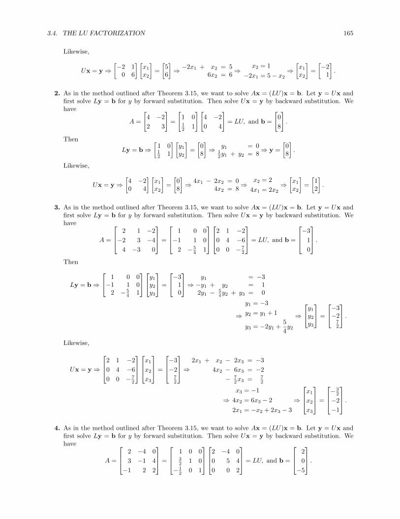
3.4. THE LU FACTORIZATION 165
Likewise,
Ux = y⇒[−2 1
0 6
] [x1
x2
]=
[56
]⇒ −2x1 + x2 = 5
6x2 = 6⇒
x2 = 1
−2x1 = 5− x2
⇒[x1
x2
]=
[−2
1
].
2. As in the method outlined after Theorem 3.15, we want to solve Ax = (LU)x = b. Let y = Ux andfirst solve Ly = b for y by forward substitution. Then solve Ux = y by backward substitution. Wehave
A =
[4 −2
2 3
]=
[1 012 1
][4 −2
0 4
]= LU, and b =
[0
8
].
Then
Ly = b⇒[
1 012 1
] [y1
y2
]=
[08
]⇒ y1 = 0
12y1 + y2 = 8
⇒ y =
[08
].
Likewise,
Ux = y⇒[4 −20 4
] [x1
x2
]=
[08
]⇒ 4x1 − 2x2 = 0
4x2 = 8⇒
x2 = 2
4x1 = 2x2
⇒[x1
x2
]=
[12
].
3. As in the method outlined after Theorem 3.15, we want to solve Ax = (LU)x = b. Let y = Ux andfirst solve Ly = b for y by forward substitution. Then solve Ux = y by backward substitution. Wehave
A =
2 1 −2
−2 3 −4
4 −3 0
=
1 0 0
−1 1 0
2 − 54 1
2 1 −2
0 4 −6
0 0 − 72
= LU, and b =
−3
1
0
.Then
Ly = b⇒
1 0 0−1 1 0
2 − 54 1
y1
y2
y3
=
−310
⇒ y1 = −3−y1 + y2 = 12y1 − 5
4y2 + y3 = 0
⇒
y1 = −3
y2 = y1 + 1
y3 = −2y1 +5
4y2
⇒
y1
y2
y3
=
−3−2
72
.Likewise,
Ux = y⇒
2 1 −2
0 4 −6
0 0 − 72
x1
x2
x3
=
−3
−272
⇒ 2x1 + x2 − 2x3 = −3
4x2 − 6x3 = −2
− 72x3 = 7
2
⇒x3 = −1
4x2 = 6x3 − 2
2x1 = −x2 + 2x3 − 3
⇒
x1
x2
x3
=
−32
−2
−1
.4. As in the method outlined after Theorem 3.15, we want to solve Ax = (LU)x = b. Let y = Ux and
first solve Ly = b for y by forward substitution. Then solve Ux = y by backward substitution. Wehave
A =
2 −4 0
3 −1 4
−1 2 2
=
1 0 032 1 0
− 12 0 1
2 −4 0
0 5 4
0 0 2
= LU, and b =
2
0
−5
.
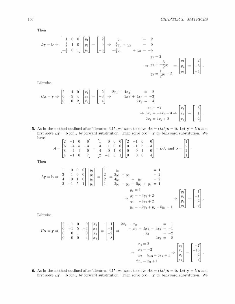
166 CHAPTER 3. MATRICES
Then
Ly = b⇒
1 0 032 1 0
− 12 0 1
y1
y2
y3
=
2
0
−5
⇒ y1 = 232y1 + y2 = 0
− 12y1 + y3 = −5
⇒
y1 = 2
y2 = −3
2y1
y3 =1
2y1 − 5
⇒
y1
y2
y3
=
2
−3
−4
.Likewise,
Ux = y⇒
2 −4 00 5 40 0 2
x1
x2
x3
=
2−3−4
⇒ 2x1 − 4x2 = 25x2 + 4x3 = −3
2x3 = −4
⇒x3 = −2
5x2 = −4x3 − 3
2x1 = 4x2 + 2
⇒
x1
x2
x3
=
3
1
−2
.5. As in the method outlined after Theorem 3.15, we want to solve Ax = (LU)x = b. Let y = Ux and
first solve Ly = b for y by forward substitution. Then solve Ux = y by backward substitution. Wehave
A =
2 −1 0 06 −4 5 −38 −4 1 04 −1 0 7
=
1 0 0 03 1 0 04 0 1 02 −1 5 1
2 −1 0 00 −1 5 −30 0 1 00 0 0 4
= LU, and b =
1221
.Then
Ly = b⇒
1 0 0 03 1 0 04 0 1 02 −1 5 1
y1
y2
y3
y4
=
1221
⇒y1 = 1
3y1 + y2 = 24y1 + y3 = 22y1 − y2 + 5y3 + y4 = 1
⇒
y1 = 1
y2 = −3y1 + 2
y3 = −4y1 + 2
y4 = −2y1 + y2 − 5y3 + 1
⇒
y1
y2
y3
y4
=
1−1−2
8
.Likewise,
Ux = y⇒
2 −1 0 00 −1 5 −30 0 1 00 0 0 4
x1
x2
x3
x4
=
1−1−2
8
⇒2x1 − x2 = 1− x2 + 5x3 − 3x4 = −1
x3 = −24x4 = 8
⇒
x4 = 2
x3 = −2
x2 = 5x3 − 3x4 + 1
2x1 = x2 + 1
⇒
x1
x2
x3
x4
=
−7−15−2
2
.
6. As in the method outlined after Theorem 3.15, we want to solve Ax = (LU)x = b. Let y = Ux andfirst solve Ly = b for y by forward substitution. Then solve Ux = y by backward substitution. We

3.4. THE LU FACTORIZATION 167
have
A =
1 4 3 0−2 −5 −1 2
3 6 −3 −4
=
1 0 0 0−2 1 0 0
3 −2 1 0−5 4 −2 1
1 4 3 00 3 5 20 0 −2 00 0 0 1
= LU, and b =
1−3−1
0
.Then
Ly = b⇒
1 0 0 0−2 1 0 0
3 −2 1 0−5 4 −2 1
y1
y2
y3
y4
=
1−3−1
0
⇒y1 = 1
−2y1 + y2 = −33y1 − 2y2 + y3 = −1−5y1 + 4y2 − 2y3 + y4 = 0
⇒
y1 = 1
y2 = 2y1 − 3
y3 = −3y1 + 2y2 − 1
y4 = 5y1 − 4y2 + 2y3
⇒
y1
y2
y3
y4
=
1−1−6−3
.Likewise,
Ux = y⇒
1 4 3 00 3 5 20 0 −2 00 0 0 1
x1
x2
x3
x4
=
1−1−6−3
⇒x1 + 4x2 + 3x3 = 1
3x2 + 5x3 + 2x4 = −1− 2x3 = −6
x4 = −3
⇒
x4 = −3
x3 = 3
3x2 = −5x3 − 2x4 − 1
x1 = −4x2 − 3x3 + 1
⇒
x1
x2
x3
x4
=
163
− 103
3
−3
.7. We use the multiplier method from Example 3.35:
A =
[1 2−3 −1
]R3−(−3R1)−−−−−−−−→
[1 20 5
]= U.
The multiplier was −3, so
L =
[1 0−3 1
].
8. We use the multiplier method from Example 3.35:
A =
[2 −43 1
]R3− 3
2R1−−−−−−→
[2 −40 7
]= U.
The multiplier was 32 , so
L =
[1 032 1
].
9. We use the multiplier method from Example 3.35:
A =
1 2 34 5 68 7 9
R2−4R1−−−−−→R3−8R1−−−−−→
1 2 30 −3 −60 −9 −15
R3−3R2−−−−−→
1 2 30 −3 −60 0 3
= U.
The multipliers were `21 = 4, `31 = 8, and `32 = 3, so we get
L =
1 0 04 1 08 3 1

168 CHAPTER 3. MATRICES
10. We use the multiplier method from Example 3.35:
A =
2 2 −14 0 43 4 4
R2−2R1−−−−−→R3− 3
2R1−−−−−−→
2 2 −10 −4 60 1 11
2
R3−(− 1
4R2)−−−−−−−−→
2 2 −10 −4 60 0 7
= U.
The multipliers were `21 = 2, `31 = 32 , and `32 = − 1
4 , so we get
L =
1 0 02 1 032 − 1
4 1
11. We use the multiplier method from Example 3.35:
A =
1 2 3 −12 6 3 00 6 −6 7−1 −2 −9 0
R2−2R1−−−−−→R3−0R1−−−−−→
R4−(−1R1)−−−−−−−−→
1 2 3 −10 2 −3 20 6 −6 70 0 −6 −1
R3−3R2−−−−−→R4−0R2−−−−−→
1 2 3 −10 2 −3 20 0 3 10 0 −6 −1
R4−(−2R3)−−−−−−−−→
1 2 3 −10 2 −3 20 0 3 10 0 0 1
= U.
The multipliers were `21 = 2, `31 = 0, `41 = −1, `32 = 3, `42 = 0, and `43 = −2, so
L =
1 0 0 02 1 0 00 3 1 0−1 0 −2 1
.12. We use the multiplier method from Example 3.35:
A =
2 2 2 1−2 4 −1 2
4 4 7 36 9 5 8
R2−(−R1)−−−−−−−→R3−2R1−−−−−→R4−3R1−−−−−→
2 2 2 10 6 1 30 0 3 10 3 −1 5
R3−0R2−−−−−→R4− 1
2R2−−−−−−→
2 2 2 10 6 1 30 0 3 10 0 − 3
272
R4−(− 12R3)
−−−−−−−−→
2 2 2 10 6 1 30 0 3 10 0 0 4
= U.
The multipliers were `21 = −1, `31 = 2, `41 = 3, `32 = 0, `42 = 12 , and `43 = − 1
2 , so
L =
1 0 0 0−1 1 0 0
2 0 1 03 1
2 − 12 1
.13. We can use the multiplier method as before to make the matrix “upper triangular”, i.e., in row echelon
form. In this case, however, the matrix is already in row echelon form, so it is equal to U , and L = I3:1 0 1 −20 3 3 10 0 0 5
=
1 0 00 1 00 0 1
1 0 1 −20 3 3 10 0 0 5
.

3.4. THE LU FACTORIZATION 169
14. We can use the multiplier method as before to make the matrix “upper triangular”, i.e., in row echelonform.
1 2 0 −1 1−2 −7 3 8 −2
1 1 3 5 20 3 −3 −6 0
R2−(−2R1)−−−−−−−−→R3−1R1−−−−−→R4−0R1−−−−−→
1 2 0 −1 10 −3 3 6 00 −1 3 6 10 3 −3 −6 0
R3− 13R2−−−−−−→
R4−(−1R2)−−−−−−−−→
1 2 0 −1 10 −3 3 6 00 0 2 4 10 0 0 0 0
= U.
The multipliers were `21 = −2, `31 = 1, `41 = 0, `32 = 13 , and `42 = −1, so
L =
1 0 0 0−2 1 0 0
1 13 1 0
0 −1 0 1
.15. In Exercise 1, we have
A =
[−2 1
2 5
]= LU =
[1 0−1 1
] [−2 1
0 6
].
Then
L−1 =1
1
[1 0
1 1
]=
[1 0
1 1
], U−1 = − 1
12
[6 −1
0 −2
]=
[− 1
2112
0 16
],
so that
A−1 = (LU)−1 = U−1L−1 =
[− 1
2112
0 16
][1 0
1 1
]=
[− 5
12112
16
16
].
16. In Exercise 4, we have
A =
2 −4 0
3 −1 4
−1 2 2
= LU =
1 0 032 1 0
− 12 0 1
2 −4 0
0 5 4
0 0 2
.To compute L−1, we adjoin the identity matrix to L and row-reduce: 1 0 0 1 0 0
32 1 0 0 1 0
− 12 0 1 0 0 1
→1 0 0 1 0 0
0 1 0 − 32 1 0
0 0 1 12 0 1
⇒ L−1 =
1 0 0
− 32 1 012 0 1
.To compute U−1, we adjoin the identity matrix to U and row-reduce:2 −4 0 1 0 0
0 5 4 0 1 0
0 0 2 0 0 1
→1 0 0 1
225 − 4
5
0 1 0 0 15 − 2
5
0 0 1 0 0 12
⇒ U−1 =
12
25 − 4
5
0 15 − 2
5
0 0 12
.Then
A−1 = (LU)−1 = U−1L−1 =
12
25 − 4
5
0 15 − 2
5
0 0 12
1 0 0
− 32 1 012 0 1
=
−12
25 − 4
5
− 12
15 − 2
514 0 1
2
.17. Using the LU decomposition from Exercise 1, we compute A−1 one column at a time using the method
outlined in the text. That is, we first solve Lyi = ei, and then solve Uxi = yi. Column 1 of A−1 is

170 CHAPTER 3. MATRICES
found as follows:
Ly1 = e1 ⇒
[1 0
−1 1
][y11
y21
]=
[1
0
]⇒ y11 = 1
−y11 + y21 = 0⇒ y1 =
[1
1
]
Ux1 = y1 ⇒
[−2 1
0 6
][x11
x21
]=
[1
1
]⇒ −2x11 + x21 = 1
6x21 = 1⇒[x]
1=
[− 5
1216
].
Use the same procedure to find the second column:
Ly2 = e2 ⇒
[1 0
−1 1
][y12
y22
]=
[0
1
]⇒ y12 = 0
−y12 + y22 = 1⇒ y2 =
[0
1
]
Ux2 = y2 ⇒
[−2 1
0 6
][x12
x22
]=
[0
1
]⇒ −2x12 + x22 = 0
6x21 = 1⇒[x]
1=
[11216
].
So
A−1 =[x1 x2
]=
[− 5
12112
16
16
].
This matches what we found in Exercise 15.
18. Using the LU decomposition from Exercise 4, we compute A−1 one column at a time using the methodoutlined in the text. That is, we first solve Lyi = ei, and then solve Uxi = yi. Column 1 of A−1 isfound as follows:
Ly1 = e1 =
1 0 032 1 0
− 12 0 1
y11
y21
y31
=
1
0
0
⇒ y11 = 132y11 + y21 = 0
− 12y11 + y31 = 0
⇒
y11
y21
y31
=
1
− 3212
Ux1 = y1 =
2 −4 0
0 5 4
0 0 2
x11
x21
x31
=
1
− 3212
⇒ 2x11 − 4x21 = 1
5x21 + 4x31 = − 32
2x31 = 12
⇒
x11
x21
x31
=
−12
− 1214
Repeat this procedure to find the second column:
Ly2 = e2 =
1 0 032 1 0
− 12 0 1
y12
y22
y32
=
0
1
0
⇒ y12 = 032y12 + y22 = 1
− 12y12 + y32 = 0
⇒
y12
y22
y32
=
0
1
0
Ux2 = y2 =
2 −4 0
0 5 4
0 0 2
x12
x22
x32
=
0
1
0
⇒ 2x12 − 4x22 = 0
5x22 + 4x32 = 1
2x32 = 0
⇒
x12
x22
x32
=
2515
0
Do this again to find the third column:
Ly3 = e3 =
1 0 032 1 0
− 12 0 1
y13
y23
y33
=
0
0
1
⇒ y13 = 032y13 + y23 = 0
− 12y13 + y33 = 1
⇒
y13
y23
y33
=
0
0
1
Ux3 = y3 =
2 −4 0
0 5 4
0 0 2
x13
x23
x33
=
0
0
1
⇒ 2x13 − 4x23 = 0
5x23 + 4x33 = 0
2x33 = 1
⇒
x13
x23
x33
=
−45
− 2512
Thus A−1 =[x1 x2 x3
]=
−12
25 − 4
5
− 12
15 − 2
514 0 1
2
; this matches what we found in Exercise 16.

3.4. THE LU FACTORIZATION 171
19. This matrix results from the identity matrix by first interchanging rows 1 and 2, and then interchangingthe (new) row 1 with row 3, so it is
E13E12 =
0 0 10 1 01 0 0
0 1 01 0 00 0 1
=
0 0 11 0 00 1 0
.Other products of elementary matrices are possible.
20. This matrix results from the identity matrix by first interchanging rows 1 and 4, and then interchangingrows 2 and 3, so it is
E14E23 =
0 0 0 10 1 0 00 0 1 01 0 0 0
1 0 0 00 0 1 00 1 0 00 0 0 1
=
0 0 0 10 0 1 00 1 0 01 0 0 0
Other products of elementary matrices are possible; for example, also P = E13E23E34.
21. To get from the given matrix to the identity matrix, perform the following exchanges:0 1 0 00 0 0 11 0 0 00 0 1 0
R1↔R3−−−−−→
1 0 0 00 0 0 10 1 0 00 0 1 0
R2↔R3−−−−−→
1 0 0 00 1 0 00 0 0 10 0 1 0
R3↔R4−−−−−→
1 0 0 00 1 0 00 0 1 00 0 0 1
Thus we can construct the given matrix P by multiplying these elementary matrices together in thereverse order:
P = E13E23E34.
Other combinations are possible.
22. To get from the given matrix to the identity matrix, perform the following exchanges:0 0 1 0 01 0 0 0 00 0 0 1 00 0 0 0 10 1 0 0 0
R1↔R2−−−−−→
1 0 0 0 00 0 1 0 00 0 0 1 00 0 0 0 10 1 0 0 0
R2↔R5−−−−−→
1 0 0 0 00 1 0 0 00 0 0 1 00 0 0 0 10 0 1 0 0
R3↔R5−−−−−→
1 0 0 0 00 1 0 0 00 0 1 0 00 0 0 0 10 0 0 1 0
R4↔R5−−−−−→
1 0 0 0 00 1 0 0 00 0 1 0 00 0 0 1 00 0 0 0 1
Thus we can construct the given matrix P by multiplying these elementary matrices together in thereverse order:
P = E12E25E35E45.
Other combinations are possible.
23. To find a PTLU factorization of A, we begin by permuting the rows of A to get it into a form thatwill result in a small number of operations to reduce to row echelon form. Since
A =
0 1 4−1 2 1
1 3 3
, we have PA =
0 1 01 0 00 0 1
0 1 4−1 2 1
1 3 3
=
−1 2 10 1 41 3 3
.

172 CHAPTER 3. MATRICES
Now follow the multiplier method from Example 3.35 to find the LU factorization of this matrix:
PA =
−1 2 10 1 41 3 3
R3−(−R1)−−−−−−−→
−1 2 10 1 40 5 4
R3−5R2−−−−−→
−1 2 10 1 40 0 −16
= U.
Then `21 = 0, `31 = −1, and `32 = 5, so that
L =
1 0 00 1 0−1 5 1
Thus
A = PTLU =
0 1 01 0 00 0 1
1 0 00 1 0−1 5 1
−1 2 10 1 40 0 −16
.24. To find a PTLU factorization of A, we begin by permuting the rows of A to get it into a form that
will result in a small number of operations to reduce to row echelon form. Since
A =
0 0 1 2−1 1 3 2
0 2 1 11 1 −1 0
, we have PA =
0 0 0 10 0 1 01 0 0 00 1 0 0
0 0 1 2−1 1 3 2
0 2 1 11 1 −1 0
=
1 1 −1 00 2 1 10 0 1 2−1 1 3 2
.Now follow the multiplier method from Example 3.35 to find the LU factorization of this matrix:
PA =
1 1 −1 00 2 1 10 0 1 2−1 1 3 2
R4−(−R1)−−−−−−−→
1 1 −1 00 2 1 10 0 1 20 2 2 2
R4−R2−−−−−→
1 1 −1 00 2 1 10 0 1 20 0 1 1
R4−R3−−−−−→
1 1 −1 00 2 1 10 0 1 20 0 0 −1
= U.
Then `41 = −1, `42 = 1, `42 = 1, and the other `ij are zero, so that
L =
1 0 0 00 1 0 00 0 1 0−1 1 1 1
.Thus
A = PTLU =
0 0 1 00 0 0 10 1 0 01 0 0 0
1 0 0 00 1 0 00 0 1 0−1 1 1 1
1 1 −1 00 2 1 10 0 1 20 0 0 −1
.25. To find a PTLU factorization of A, we begin by permuting the rows of A to get it into a form that
will result in a small number of operations to reduce to row echelon form. Since
A =
0 −1 1 3−1 1 1 2
0 1 −1 10 0 1 1
, we have PA =
0 1 0 01 0 0 00 0 0 10 0 1 0
0 −1 1 3−1 1 1 2
0 1 −1 10 0 1 1
=
−1 1 1 2
0 −1 1 30 0 1 10 1 −1 1
.

3.4. THE LU FACTORIZATION 173
Now follow the multiplier method from Example 3.35 to find the LU factorization of this matrix:
PA =
−1 1 1 2
0 −1 1 30 0 1 10 1 −1 1
R4−(−R2)−−−−−−−→
−1 1 1 2
0 −1 1 30 0 1 10 0 0 4
= U.
Then `42 = −1 and the other `ij are zero, so that
L =
1 0 0 00 1 0 00 0 1 00 −1 0 1
.Thus
A = PTLU =
0 1 0 01 0 0 00 0 0 10 0 1 0
1 0 0 00 1 0 00 0 1 00 −1 0 1
−1 1 1 2
0 −1 1 30 0 1 10 0 0 4
.26. From the text, a permutation matrix consists of the rows of the identity matrix written in some order.
So each row and each column of a permutation matrix has exactly one 1 in it, and the remaining entriesin that row or column are zero. Thus there are n choices for the column containing the 1 in the firstrow; once that is chosen, there are n − 1 choices for the column to contain the 1 in the second row.Next, there are n− 2 choices in the third row. Continuing, we decrease the number of choices by oneeach time, until there is just one choice in the last row. Multiplying all these together gives the totalnumber of choices, i.e., the number of n×n permutation matrices, which is n·(n−1)·(n−2) · · · 2·1 = n!.
27. To solve Ax = PTLUx = b, multiply both sides by P to get LUx = Pb. Now compute Pb, which is apermutation of the rows of b, and solve the resulting equation by the method outlined after Theorem3.15:
PT =
0 1 01 0 00 0 1
⇒ P =
0 1 01 0 00 0 1
⇒ Pb =
0 1 01 0 00 0 1
115
=
115
.Then
Ly = Pb⇒
1 0 0
0 1 012 − 1
2 1
y1
y2
y3
=
1
1
5
⇒ y1 = 1
y2 = 112y1 − 1
2y2 + y3 = 5
⇒
y1 = 1
y2 = 1
y3 = 5− 1
2y1 +
1
2y2
⇒
y1
y2
y3
=
1
1
5
.Likewise,
Ux = y⇒
2 3 20 1 −10 0 − 5
2
x1
x2
x3
=
115
⇒ 2x1 + 3x2 + 2x3 = 1x2 − x3 = 1− 5
2x3 = 5
⇒x3 = −2
x2 = x3 + 1
2x1 = 1− 3x2 − 2x3
⇒ x =
x1
x2
x3
=
4
−1
−2
.

174 CHAPTER 3. MATRICES
28. To solve Ax = PTLUx = b, multiply both sides by P to get LUx = Pb. Now compute Pb, which is apermutation of the rows of b, and solve the resulting equation by the method outlined after Theorem3.15:
PT =
0 0 11 0 00 1 0
⇒ P =
0 1 00 0 11 0 0
⇒ Pb =
0 1 00 0 11 0 0
16−4
4
=
−44
16
.Then
Ly = Pb⇒
1 0 01 1 02 −1 1
y1
y2
y3
=
−44
16
⇒ y1 = −4y1 + y2 = 4
2y1 − y2 + y3 = 16
⇒y1 = −4
y2 = 4− y1
y3 = 16− 2y1 + y2
⇒
y1
y2
y3
=
−4
8
32
.Likewise,
Ux = y⇒
4 1 20 −1 10 0 2
x1
x2
x3
=
−48
32
⇒ 4x1 + x2 + 2x3 = −4− x2 + x3 = 8
2x3 = 32
⇒x3 = 16
x2 = x3 − 8
4x1 = −x2 − 2x3 − 4
⇒ x =
x1
x2
x3
=
−11
8
16
.29. Let A = (aij) and B = (bij) be unit lower triangular n× n matrices, so that
aij = bij =
0 i < j
1 i = j
∗ i > j
(where of course the ∗’s maybe different for A and B). Then if C = (cij) = AB, we have
cij = ai1b1j + ai2b2j + · · ·+ ai(j−1)b(j−1)j + aijbjj + · · ·+ ainbnj .
If i < j, then all the terms up through ai(j−1)b(j−1)j since the b’s are zero, and all terms from the nextterm to the end are zero since the a’s are zero.
If i = j, then all the terms up through ai(j−1)b(j−1)j since the b’s are zero, the aijbjj = ajjbjj term is1, and all terms from the next term to the end are zero since the a’s are zero.
Finally, if i > j, multiple terms in the sum may be nonzero.
Thus we get
cij =
0 i < j
1 i = j
∗ i > j
so that C is lower unit triangular as well.
30. To invert L, we row-reduce[L I
]:
1 0 · · · 0 1 0 · · · 0∗ 1 · · · 0 0 1 · · · 0...
.... . .
......
.... . .
...∗ ∗ · · · 1 0 0 · · · 1
.
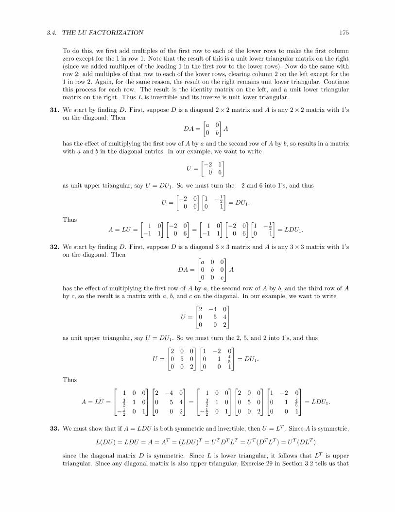
3.4. THE LU FACTORIZATION 175
To do this, we first add multiples of the first row to each of the lower rows to make the first columnzero except for the 1 in row 1. Note that the result of this is a unit lower triangular matrix on the right(since we added multiples of the leading 1 in the first row to the lower rows). Now do the same withrow 2: add multiples of that row to each of the lower rows, clearing column 2 on the left except for the1 in row 2. Again, for the same reason, the result on the right remains unit lower triangular. Continuethis process for each row. The result is the identity matrix on the left, and a unit lower triangularmatrix on the right. Thus L is invertible and its inverse is unit lower triangular.
31. We start by finding D. First, suppose D is a diagonal 2× 2 matrix and A is any 2× 2 matrix with 1’son the diagonal. Then
DA =
[a 00 b
]A
has the effect of multiplying the first row of A by a and the second row of A by b, so results in a matrixwith a and b in the diagonal entries. In our example, we want to write
U =
[−2 1
0 6
]as unit upper triangular, say U = DU1. So we must turn the −2 and 6 into 1’s, and thus
U =
[−2 0
0 6
] [1 − 1
20 1
]= DU1.
Thus
A = LU =
[1 0−1 1
] [−2 0
0 6
]=
[1 0−1 1
] [−2 0
0 6
] [1 − 1
20 1
]= LDU1.
32. We start by finding D. First, suppose D is a diagonal 3× 3 matrix and A is any 3× 3 matrix with 1’son the diagonal. Then
DA =
a 0 00 b 00 0 c
Ahas the effect of multiplying the first row of A by a, the second row of A by b, and the third row of Aby c, so the result is a matrix with a, b, and c on the diagonal. In our example, we want to write
U =
2 −4 00 5 40 0 2
as unit upper triangular, say U = DU1. So we must turn the 2, 5, and 2 into 1’s, and thus
U =
2 0 00 5 00 0 2
1 −2 00 1 4
50 0 1
= DU1.
Thus
A = LU =
1 0 032 1 0
− 12 0 1
2 −4 0
0 5 4
0 0 2
=
1 0 032 1 0
− 12 0 1
2 0 0
0 5 0
0 0 2
1 −2 0
0 1 45
0 0 1
= LDU1.
33. We must show that if A = LDU is both symmetric and invertible, then U = LT . Since A is symmetric,
L(DU) = LDU = A = AT = (LDU)T = UTDTLT = UT (DTLT ) = UT (DLT )
since the diagonal matrix D is symmetric. Since L is lower triangular, it follows that LT is uppertriangular. Since any diagonal matrix is also upper triangular, Exercise 29 in Section 3.2 tells us that
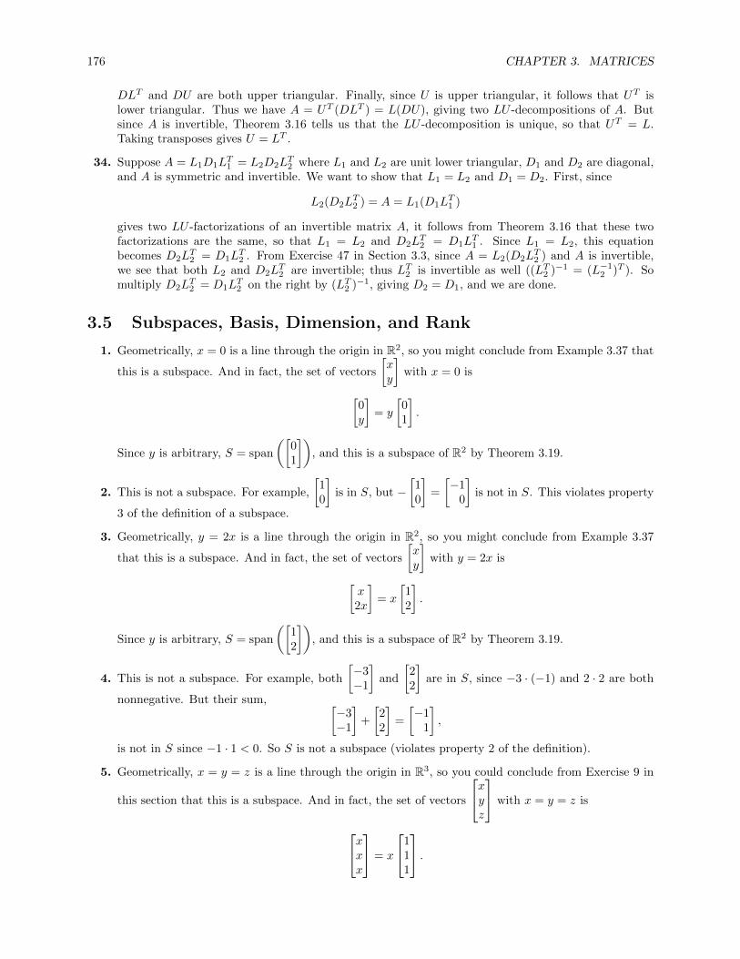
176 CHAPTER 3. MATRICES
DLT and DU are both upper triangular. Finally, since U is upper triangular, it follows that UT islower triangular. Thus we have A = UT (DLT ) = L(DU), giving two LU -decompositions of A. Butsince A is invertible, Theorem 3.16 tells us that the LU -decomposition is unique, so that UT = L.Taking transposes gives U = LT .
34. Suppose A = L1D1LT1 = L2D2L
T2 where L1 and L2 are unit lower triangular, D1 and D2 are diagonal,
and A is symmetric and invertible. We want to show that L1 = L2 and D1 = D2. First, since
L2(D2LT2 ) = A = L1(D1L
T1 )
gives two LU -factorizations of an invertible matrix A, it follows from Theorem 3.16 that these twofactorizations are the same, so that L1 = L2 and D2L
T2 = D1L
T1 . Since L1 = L2, this equation
becomes D2LT2 = D1L
T2 . From Exercise 47 in Section 3.3, since A = L2(D2L
T2 ) and A is invertible,
we see that both L2 and D2LT2 are invertible; thus LT2 is invertible as well ((LT2 )−1 = (L−1
2 )T ). Somultiply D2L
T2 = D1L
T2 on the right by (LT2 )−1, giving D2 = D1, and we are done.
3.5 Subspaces, Basis, Dimension, and Rank
1. Geometrically, x = 0 is a line through the origin in R2, so you might conclude from Example 3.37 that
this is a subspace. And in fact, the set of vectors
[xy
]with x = 0 is
[0y
]= y
[01
].
Since y is arbitrary, S = span
([01
]), and this is a subspace of R2 by Theorem 3.19.
2. This is not a subspace. For example,
[10
]is in S, but −
[10
]=
[−1
0
]is not in S. This violates property
3 of the definition of a subspace.
3. Geometrically, y = 2x is a line through the origin in R2, so you might conclude from Example 3.37
that this is a subspace. And in fact, the set of vectors
[xy
]with y = 2x is
[x2x
]= x
[12
].
Since y is arbitrary, S = span
([12
]), and this is a subspace of R2 by Theorem 3.19.
4. This is not a subspace. For example, both
[−3−1
]and
[22
]are in S, since −3 · (−1) and 2 · 2 are both
nonnegative. But their sum, [−3−1
]+
[22
]=
[−1
1
],
is not in S since −1 · 1 < 0. So S is not a subspace (violates property 2 of the definition).
5. Geometrically, x = y = z is a line through the origin in R3, so you could conclude from Exercise 9 in
this section that this is a subspace. And in fact, the set of vectors
xyz
with x = y = z is
xxx
= x
111
.

3.5. SUBSPACES, BASIS, DIMENSION, AND RANK 177
Since x is arbitrary, S = span
111
, and this is a subspace of R3 by Theorem 3.19.
6. Geometrically, this is a line in R3 lying in the xz-plane and passing through the origin, so Exercise 9
in this section implies that it is a subspace. The set of vectors
xyz
satisfying these conditions is
x02x
= x
102
.
Since x is arbitrary, S = span
102
, and this is a subspace of R3 by Theorem 3.19.
7. This is a plane in R3, but it does not pass through the origin since (0, 0, 0) does not satisfy the equation.So condition 1 in the definition is violated, and this is not a subspace.
8. This is not a subspace. For example 101
∈ S and
012
∈ Ssince for the first vector |1− 0| = |0− 1| and for the second |0− 1| = |1− 2|. But their sum,1
01
+
012
=
113
/∈ S
since |1− 1| 6= |1− 3|.
9. If a line ` passes through the origin, then it has the equation x = 0+ td = td, so that the set of pointson ` is just span(d). Then Theorem 3.19 implies that ` is a subspace of R3. (Note that we did not usethe assumption that the vectors lay in R3; in fact this conclusion holds in any Rn for n ≥ 1.)
10. This is not a subspace of R2. For example, (1, 0) ∈ S and (0, 1) ∈ S, but their sum, (1, 1), is not in Ssince it does not lie on either axis.
11. As in Example 3.41, b is in col(A) if and only if the augmented matrix
[A b
]=
[1 0 −1 31 1 1 2
]is consistent as a linear system. So we row-reduce that augmented matrix:[
1 0 −1 31 1 1 2
]R2−R1−−−−−→
[1 0 −1 30 1 2 −1
].
This matrix is in row echelon form and has no zero rows, so the system is consistent and thus b ∈ col(A).
Using Example 3.41, w is in row(A) if and only if the matrix
[Aw
]=
1 0 −11 1 1−1 1 1

178 CHAPTER 3. MATRICES
can be row-reduced to a matrix whose last row is zero by operations excluding row interchangesinvolving the last row. Thus 1 0 −1
1 1 1−1 1 1
R2−R1−−−−−→R3+R1−−−−−→
1 0 −10 1 20 1 0
R3−R2−−−−−→
1 0 −10 1 20 0 −2
This matrix is in row echelon form and has no zero rows, so we cannot make the last row zero. Thusw /∈ row(A).
12. Using Example 3.41, b is in col(A) if and only if the augmented matrix
[A b
]=
1 1 −3 10 2 1 11 −1 −4 0
is consistent as a linear system. So we row-reduce that augmented matrix:1 1 −3 1
0 2 1 1
1 −1 −4 0
R3−R1−−−−−→
1 1 −3 1
0 2 1 1
0 −2 −1 −1
R3+R2−−−−−→
1 1 −3 1
0 2 1 1
0 0 0 0
12R2−−−→
1 1 −3 1
0 1 12
12
0 0 0 0
The linear system has a solution (in fact, an infinite number of them), so is consistent. Thus b is incol(A).
Using Example 3.41, w is in row(A) if and only if the matrix
[Aw
]=
1 1 −30 2 11 −1 −42 4 −5
can be row-reduced to a matrix whose last row is zero by operations excluding row interchangesinvolving the last row. Thus
1 1 −30 2 11 −1 −42 4 −5
R3−R1−−−−−→R4−2R1−−−−−→
1 1 −30 2 10 −2 −10 2 1
R4+R3−−−−−→
1 1 −30 2 10 −2 −10 0 0
Thus w is in row(A).
13. As in the remarks following Example 3.41, we determine whether w is in row(A) using col(AT ). Tosay w is in row(A) means that wT is in col(A), so we form the augmented matrix and row-reduce tosee if the system has a solution:
[AT wT
]=
1 1 −10 1 1−1 1 1
R3+R2−−−−−→
1 1 −10 1 10 2 0
R2− 1
2R3−−−−−−→
1 1 −10 0 10 2 0
R2↔R3−−−−−→
1 1 −10 2 00 0 1
This matrix has a row that is all zeros except for the final column, so the system is inconsistent. ThuswT /∈ col(AT ) and thus w /∈ row(A).
14. As in the remarks following Example 3.41, we determine whether w is in row(A) using col(AT ). Tosay w is in row(A) means that wT is in col(A), so we form the augmented matrix and row-reduce to

3.5. SUBSPACES, BASIS, DIMENSION, AND RANK 179
see if the system has a solution:
[AT wT
]=
1 0 1 21 2 −1 4−3 1 −4 −5
R2−R1−−−−−→R3+3R1−−−−−→
1 0 1 20 2 −2 20 1 −1 1
12R2−−−→
1 0 1 20 1 −1 10 1 −1 1
R3−R2−−−−−→
1 0 1 20 1 −1 10 0 0 0
.This is in row reduced form, and the final row consists of all zeros. This is a consistent system, so thatwT ∈ col(AT ) and thus w ∈ row(A).
15. To check if v is in null(A), we need only multiply A by v:
Av =
[1 0 −11 1 1
]−13−1
=
[01
]6= 0,
so that v /∈ null(A).
16. To check if v is in null(A), we need only multiply A by v:
Av =
1 1 −30 2 11 −1 −4
7−1
2
=
000
= 0,
so that v ∈ null(A).
17. We follow the comment after Example 3.48. Start by finding the reduced row echelon form of A:[1 0 −11 1 1
]R2−R1−−−−−→
[1 0 −10 1 2
]Thus a basis for row(A) is given by
{[1 0 −1
],[0 1 2
]}.
A basis for col(A) is given by the column vectors of the original matrix A corresponding to the leading1s in the row-reduced matrix, so a basis for col(A) is{[
11
],
[01
]}.
Finally, from the row-reduced form, the solutions to Ax = 0 where
x =
x1
x2
x3
can be found by noting that x3 is a free variable; setting it to t and then solving for the other twovariables gives x1 = t and x2 = −2t. Thus a basis for the nullspace of A is given by
x =
1−2
1
.

180 CHAPTER 3. MATRICES
18. We follow the comment after Example 3.48. Start by finding the reduced row echelon form of A:1 1 −3
0 2 1
1 −1 −4
R3−R1−−−−−→
1 1 −3
0 2 1
0 −2 −1
R3+R2−−−−−→
1 1 −3
0 2 1
0 0 0
12R2−−−→
1 1 −3
0 1 12
0 0 0
R1−R2−−−−−→
1 0 − 7
2
0 1 12
0 0 0
Thus a basis for row(A) is given by{[
1 0 − 72
],[0 1 1
2
]}or, clearing fractions,
{[2 0 −7
],[0 2 1
]}.
Since the row-reduction did not involve any row exchanges, a basis for row(A) is also given by the rowsof A corresponding to nonzero rows in the reduced matrix:{[
1 1 −3],[0 2 1
]}.
A basis for col(A) is then given by the original column vectors of A corresponding to the columnscontaining the leading 1s in the row-reduced matrix; thus a basis for col(A) is given by
101
, 1
2−1
Finally, from the row-reduced form, the solutions of Ax = 0 where
x =
x1
x2
x3
can be found by noting that x3 is a free variable; we set it to t, and then solving for the other twovariables in terms of t to get x1 = 7
2 t and x2 = − 12 t. Thus a basis for the nullspace of A is given by
x =
72
− 12
1
or
7
−1
2
19. We follow the comment after Example 3.48. Start by finding the reduced row echelon form of A:1 1 0 1
0 1 −1 10 1 −1 −1
R3−R2−−−−−→
1 1 0 10 1 −1 10 0 0 −2
− 1
2R3−−−−→
1 1 0 10 1 −1 10 0 0 1
R1−R3−−−−−→R2−R3−−−−−→
1 1 0 00 1 −1 00 0 0 1
R1−R2−−−−−→1 0 1 0
0 1 −1 00 0 0 1
Thus a basis for row(A) is given by{[
1 0 1 0],[0 1 −1 0
],[0 0 0 1
]}.
Since the row-reduction did not involve any row exchanges, a basis for row(A) is also given by the rowsof A corresponding to nonzero rows in the reduced matrix; since all the rows are nonzero, the rows ofA form a basis for row(A).
A basis for col(A) is then given by the original column vectors of A corresponding to the columnscontaining the leading 1s in the row-reduced matrix; thus a basis for col(A) is given by
100
,1
11
, 1
1−1

3.5. SUBSPACES, BASIS, DIMENSION, AND RANK 181
Finally, from the row-reduced form, the solutions of Ax = 0 where
x =
x1
x2
x3
x4
can be found by noting that x3 is a free variable; we set it to t. Also, x4 = 0; solving for the other twovariables in terms of t gives x1 = −t and x2 = t. Thus a basis for the nullspace of A is given by
x =
−1
110
.20. We follow the comment after Example 3.48. Start by finding the reduced row echelon form of A: 2 −4 0 2 1
−1 2 1 2 3
1 −2 1 4 4
R1↔R3−−−−−→
1 −2 1 4 4
−1 2 1 2 3
2 −4 0 2 1
R2+R1−−−−−→R3−2R1−−−−−→
1 −2 1 4 4
0 0 2 6 7
0 0 −2 −6 −7
R3+R2−−−−−→1 −2 1 4 4
0 0 2 6 7
0 0 0 0 0
12R2−−−→
1 −2 1 4 4
0 0 1 3 72
0 0 0 0 0
R1−R2−−−−−→
1 −2 0 1 12
0 0 1 3 72
0 0 0 0 0
Thus a basis for row(A) is given by the nonzero rows of the reduced matrix, which after clearingfractions are {[
2 −4 0 2 1],[0 0 2 6 7
]}.
A basis for col(A) is then given by the original column vectors of A corresponding to the columnscontaining the leading 1s in the row-reduced matrix; thus a basis for col(A) is given by
2−1
1
,0
11
.
Finally, from the row-reduced form, the solutions of Ax = 0 where
x =
x1
x2
x3
x4
x5
can be found by noting that x2 = s, x4 = t, and x5 = u are free variables. Solving for the other twovariables gives x1 = 2s− t− 1
2u and x3 = −3t− 72u. Thus the nullspace of A is given by
2s− t+ 1
2us
−3t− 72u
tu
=
s
21000
+ t
−1
0−3
10
+ u
− 1
20− 7
201
= span
21000
,−1
0−3
10
,− 1
20− 7
201
.
Clearing fractions, we get for a basis for the nullspace of A
21000
,−1
0−3
10
,−1
0−7
02
.

182 CHAPTER 3. MATRICES
21. Since row(A) = col(AT ) and col(A) = row(AT ), it suffices to find the row and column spaces of AT .Then
AT =
1 10 1−1 1
→1 0
0 10 0
,so that the column space of AT is given by the columns of AT corresponding to columns of this matrixcontaining a leading 1, so
col(AT ) =
1
0−1
,1
11
⇒ row(A) ={[
1 0 −1],[1 1 1
]}.
The row space of AT is given by the nonzero rows of the reduced matrix, so
row(AT ) ={[
1 0],[0 1
]}⇒ col(A) =
{[10
],
[01
]}.
22. Since row(A) = col(AT ) and col(A) = row(AT ), it suffices to find the row and column spaces of AT .Then
AT =
1 0 11 2 −1−3 1 −4
→1 0 1
0 1 −10 0 0
,so that the column space of AT is given by the columns of AT corresponding to columns of the reducedmatrix containing a leading 1, so
col(AT ) =
1
1−3
,0
21
⇒ row(A) ={[
1 1 −3],[0 2 1
]}.
The row space of AT is given by the nonzero rows of the reduced matrix, so
row(AT ) ={[
1 0 1],[0 1 −1
]}⇒ col(A) =
1
01
, 0
1−1
.
23. Since row(A) = col(AT ) and col(A) = row(AT ), it suffices to find the row and column spaces of AT .Then
AT =
1 0 11 1 10 −1 −11 1 −1
→
1 0 00 1 00 0 10 0 0
,so that the column space of AT is given by the columns of AT corresponding to columns of the reducedmatrix containing a leading 1, so
col(AT ) =
1101
,
01−1
1
,
01−1−1
⇒ row(A) =
{[1 1 0 1
],[0 1 −1 1
],[0 1 −1 −1
]}.
The row space of AT is given by the nonzero rows of the reduced matrix, so
row(AT ) ={[
1 0 0],[0 1 0
],[0 0 1
]}⇒ col(A) =
1
00
,0
10
,0
01
.

3.5. SUBSPACES, BASIS, DIMENSION, AND RANK 183
24. Since row(A) = col(AT ) and col(A) = row(AT ), it suffices to find the row and column spaces of AT .Then
AT =
2 −1 1−4 2 −2
0 1 12 2 41 3 4
→
1 0 10 1 10 0 00 0 00 0 0
,so that the column space of AT is given by the columns of AT corresponding to columns of the reducedmatrix containing a leading 1, so
col(AT ) =
2−4
021
,−1
2123
⇒ row(A) =
{[2 −4 0 2 1
],[−1 2 1 2 3
]}.
The row space of AT is given by the nonzero rows of the reduced matrix, so
row(AT ) ={[
1 0 1],[0 1 1
]}⇒ col(A) =
1
01
,0
11
.
25. There is no reason to expect the bases for the row and column spaces found in Exercises 17 and 21 tobe the same, since we used different methods to find them. What is important is that they should spanthe same subspaces. The basis for the row space found in Exercise 17 was {
[1 0 −1
],[0 1 2
]},
and Exercise 21 gave {[1 0 −1
],[1 1 1
]}. Since the first basis vector is the same, in order to
show the subspaces are the same it suffices to see that[0 1 2
]is in the span of the second basis,
and that[1 1 1
]is in the span of the first basis. But[
0 1 2]
= −[1 0 −1
]+[1 1 1
],
[1 1 1
]=[1 0 −1
]+[0 1 2
].
So the two bases span the same row space. Similarly, the basis for the two column spaces were
Exercise 17:
{[11
],
[01
]}, Exercise 21:
{[10
],
[01
]}.
Here the second basis vectors are the same, and since[11
]=
[10
]+
[01
],
[10
]=
[11
]−[01
],
each basis vector is a linear combination of the vectors in the other basis, so they span the same columnspace.
26. There is no reason to expect the bases for the row and column spaces found in Exercises 18 and 22 tobe the same, since we used different methods to find them. What is important is that they should spanthe same subspaces. The basis for the row space found in Exercise 18 was {
[2 0 −7
],[0 2 1
]},
and Exercise 22 gave {[1 1 −3
],[0 2 1
]}. Since the second basis vector is the same, in order to
show the subspaces are the same it suffices to see that[2 0 −7
]is in the span of the second basis,
and that[1 1 −3
]is in the span of the first basis. But[
2 0 −7]
= 2[1 1 −3
]−[0 2 1
],
[1 1 −3
]=
1
2
[2 0 −7
]+
1
2
[0 2 1
].
So the two bases span the same row space. Similarly, the basis for the two column spaces were
Exercise 18:
1
01
, 1
2−1
, Exercise 22:
1
01
, 0
1−1
.
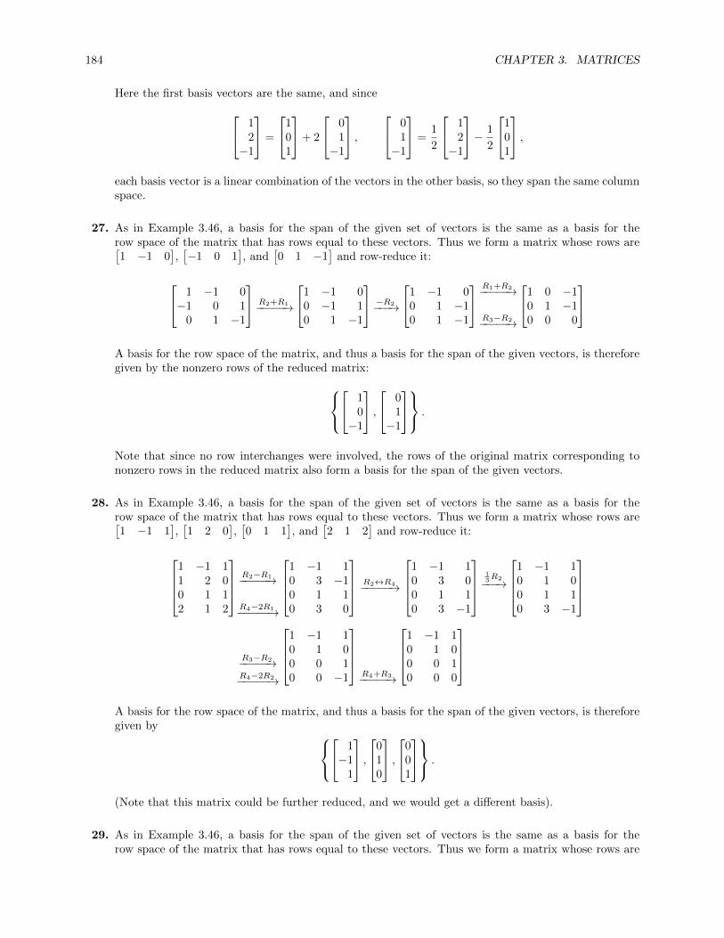
184 CHAPTER 3. MATRICES
Here the first basis vectors are the same, and since 12−1
=
101
+ 2
01−1
, 0
1−1
=1
2
12−1
− 1
2
101
,each basis vector is a linear combination of the vectors in the other basis, so they span the same columnspace.
27. As in Example 3.46, a basis for the span of the given set of vectors is the same as a basis for therow space of the matrix that has rows equal to these vectors. Thus we form a matrix whose rows are[1 −1 0
],[−1 0 1
], and
[0 1 −1
]and row-reduce it:
1 −1 0−1 0 1
0 1 −1
R2+R1−−−−−→
1 −1 00 −1 10 1 −1
−R2−−−→
1 −1 00 1 −10 1 −1
R1+R2−−−−−→
R3−R2−−−−−→
1 0 −10 1 −10 0 0
A basis for the row space of the matrix, and thus a basis for the span of the given vectors, is thereforegiven by the nonzero rows of the reduced matrix:
10−1
, 0
1−1
.
Note that since no row interchanges were involved, the rows of the original matrix corresponding tononzero rows in the reduced matrix also form a basis for the span of the given vectors.
28. As in Example 3.46, a basis for the span of the given set of vectors is the same as a basis for therow space of the matrix that has rows equal to these vectors. Thus we form a matrix whose rows are[1 −1 1
],[1 2 0
],[0 1 1
], and
[2 1 2
]and row-reduce it:
1 −1 11 2 00 1 12 1 2
R2−R1−−−−−→
R4−2R1−−−−−→
1 −1 10 3 −10 1 10 3 0
R2↔R4−−−−−→
1 −1 10 3 00 1 10 3 −1
13R2−−−→
1 −1 10 1 00 1 10 3 −1
R3−R2−−−−−→R4−2R2−−−−−→
1 −1 10 1 00 0 10 0 −1
R4+R3−−−−−→
1 −1 10 1 00 0 10 0 0
A basis for the row space of the matrix, and thus a basis for the span of the given vectors, is thereforegiven by
1−1
1
,0
10
,0
01
.
(Note that this matrix could be further reduced, and we would get a different basis).
29. As in Example 3.46, a basis for the span of the given set of vectors is the same as a basis for therow space of the matrix that has rows equal to these vectors. Thus we form a matrix whose rows are

3.5. SUBSPACES, BASIS, DIMENSION, AND RANK 185
[2 −3 1
],[1 −1 0
],[4 −4 1
]and row-reduce it:2 −3 1
1 −1 04 −4 1
R1↔R2−−−−−→
1 −1 02 −3 14 −4 1
R2−2R1−−−−−→R3−4R1−−−−−→
1 −1 00 −1 10 −2 1
−R2−−−→
1 −1 00 1 −10 −2 1
R3+2R2−−−−−→
1 −1 00 1 −10 0 −1
−R3−−−→
1 −1 00 1 −10 0 1
R2+R3−−−−−→
1 −1 00 1 00 0 1
R1+R2−−−−−→
1 0 00 1 00 0 1
A basis for the row space of the matrix, and thus a basis for the span of the given vectors, is thereforegiven by
{[1 0 0
],[0 1 0
],[0 0 1
]}
(Note that as soon as we got to the first matrix on the second line above, we could have concluded thatthe reduced matrix would have no zero rows; since it was 3× 3, it would thus be the identity matrix,so that we could immediately write down the basis above, or simply use the basis given by the rows ofthat matrix).
30. As in Example 3.46, a basis for the span of the given set of vectors is the same as a basis for therow space of the matrix that has rows equal to these vectors. Thus we form a matrix whose rows are[0 1 −2 1
],[3 1 −1 0
],[2 1 5 1
]and row-reduce it:
0 1 −2 1
3 1 −1 0
2 1 5 1
R1↔R2−−−−−→
3 1 −1 0
0 1 −2 1
2 1 5 1
13R1−−−→
1 1
3 − 13 0
0 1 −2 1
2 1 5 1
R3−2R1−−−−−→
1 1
3 − 13 0
0 1 −2 1
0 13
173 1
R3− 1
3R2−−−−−−→
1 1
3 − 13 0
0 1 −2 1
0 0 193
23
319R3−−−→
1 1
3 − 13 0
0 1 −2 1
0 0 1 219
Although this matrix could be reduced further, we already have a basis for the row space:[
1 13 − 1
3 0],[0 1 −2 1
],[0 0 1 2
19
],
or [3 1 −1 0
],[0 1 −2 1
],[0 0 19 2
].
31. If, as in Exercise 29, we form the matrix whose rows are those vectors and row-reduce it, we getthe identity matrix (see Exercise 29). Because there were no row exchanges, the rows of the originalmatrix corresponding to nonzero rows in the row-reduced matrix form a basis for the span of thevectors (because there were no row exchanges). Thus a basis consists of all three given vectors:[
2 −3 1],[1 −1 0
],[4 −4 1
].
32. If, as in Exercise 30, we form the matrix whose rows are those vectors and row-reduce it, we get amatrix with no zero rows. Thus the rank of the matrix is 3, so the rows are linearly independent, so abasis consists of all three row vectors:[
0 1 −2 1],[3 1 −1 0
],[2 1 5 1
].

186 CHAPTER 3. MATRICES
33. If R is a matrix in echelon form, then row(R) is the span of the rows of R, by definition. But nonzerorows of R are linearly independent, since their first entries are in different columns, so those nonzerorows form a basis for row(R) (they span, and are linearly independent).
34. col(A) is the span of the columns of A by definition. If the columns of A are also linearly independent,then they form a basis for col(A) by definition of “basis”.
35. The rank of A is the number of vectors in a basis for either row(A) or col(A), by definition. FromExercise 17, row(A) has two vectors in its basis, so rank(A) = 2. Then nullity(A) is the number ofcolumns minus the rank, or 3− 2 = 1.
36. The rank of A is the number of vectors in a basis for either row(A) or col(A), by definition. FromExercise 18, row(A) has two vectors in its basis, so rank(A) = 2. Then nullity(A) is the number ofcolumns minus the rank, or 3− 2 = 1.
37. The rank of A is the number of vectors in a basis for either row(A) or col(A), by definition. FromExercise 19, row(A) has three vectors in its basis, so rank(A) = 3. Then nullity(A) is the number ofcolumns minus the rank, or 4− 3 = 1.
38. The rank of A is the number of vectors in a basis for either row(A) or col(A), by definition. FromExercise 20, row(A) has two vectors in its basis, so rank(A) = 2. Then nullity(A) is the number ofcolumns minus the rank, or 5− 2 = 3.
39. Since nullity(A) > 0, the equation Ax = 0 has a nontrivial solution xT =[c1 c2 · · · cn
], where at
least one ci 6= 0. Then Ax =∑ciai = 0. Since at least one ci 6= 0, this shows that the columns of A
are linearly dependent.
40. Since rank(A) is at most the number of columns of A and also at most the number of rows of A, inthis case rank(A) ≤ 2. Thus any row-reduced form of A will have at least 4− 2 = 2 zero rows, whichmeans that some row of A is a linear combination of the other rows, so that the rows of A are linearlydependent.
41. Since rank(A) is at most the number of columns of A and also at most the number of rows of A, inthis case rank(A) ≤ 5 and rank(A) ≤ 3, so that rank(A) ≤ 3 and its possible values are 0, 1, 2, and 3.Using the Rank Theorem, we know that
nullity(A) = n− rank(A) = 5− rank(A), so that nullity(A) = 5, 4, 3, or 2.
42. Since rank(A) is at most the number of columns of A and also at most the number of rows of A, inthis case rank(A) ≤ 2 and rank(A) ≤ 4, so that rank(A) ≤ 2 and its possible values are 0, 1, and 2.Using the Rank Theorem, we know that
nullity(A) = 2− rank(A) = 1− rank(A), so that nullity(A) = 2, 1, or 0.
43. First row-reduce A: 1 2 a−2 4a 2a −2 1
R2+2R1−−−−−→R3−aR1−−−−−→
1 2 a0 4a+ 4 2a+ 20 −2a− 2 1− a2
R2+ 1
2R2−−−−−−→
1 2 a0 4a+ 4 2a+ 20 0 −a2 + a+ 2
If a = −1, then we have 1 2 −1
0 0 00 0 0
so that rank(A) = 1.
If a = 2, then we have 1 2 20 12 60 0 0
so that rank(A) = 2.
Otherwise, the row-reduced matrix has all rows nonzero, so that rank(A) = 3.

3.5. SUBSPACES, BASIS, DIMENSION, AND RANK 187
44. First row-reduce A: a 2 −13 3 −2−2 −1 a
R1↔R3−−−−−→
−2 −1 a3 3 −2a 2 −1
R1+R2−−−−−→1 2 a− 2
3 3 −2a 2 −1
R2−3R1−−−−−→R3−aR2−−−−−→
1 2 a− 20 −3 4− 3a0 2− 2a −a2 + 2a− 1
− 13R2−−−−→
1 2 a− 20 1 a− 4
30 2− 2a −a2 + 2a− 1
R3−(2−2a)R2−−−−−−−−−→
1 2 a− 20 1 a− 4
30 0 (a− 1)
(a− 5
3
)
The first two rows are always nonzero. If a = 1 or a = 53 , then the bottom row is zero, so that
rank(A) = 2. Otherwise, all three rows are nonzero and rank(A) = 3.
45. As in example 3.52, 110
,1
01
,0
11
form a basis for R3 if and only if the matrix with those vectors as its rows has rank 3. Row-reducethat matrix: 1 1 0
1 0 10 1 1
R2−R1−−−−−→
1 1 00 −1 10 1 1
R3+R2−−−−−→
1 1 00 −1 10 0 2
Since the matrix has rank 3 (it has no nonzero rows and is in echelon form), the vectors are linearlyindependent; since there are three of them, they form a basis for R3.
46. As in example 3.52, 1−1
3
,−1
51
, 1−3
1
form a basis for R3 if and only if the matrix with those vectors as its rows has rank 3. Row-reducethat matrix: 1 −1 3
−1 5 11 −3 1
R2+2R1−−−−−→R3−R1−−−−−→
1 −1 30 4 40 −2 −2
R2+2R3−−−−−→
1 −1 30 0 00 −2 −2
Since the matrix does not have rank 3, it follows that these vectors do not form a basis for R3. (Infact,
−
1−1
3
+
−151
+ 2
1−3
1
=
000
,so the vectors are linearly dependent.)
47. As in example 3.52, 1110
,
1101
,
1011
,
0111

188 CHAPTER 3. MATRICES
form a basis for R4 if and only if the matrix with those vectors as its rows has rank 4. Row-reducethat matrix:
1 1 1 01 1 0 11 0 1 10 1 1 1
R2−R1−−−−−→R3−R1−−−−−→
1 1 1 00 0 −1 10 −1 0 10 1 1 1
R4↔R2−−−−−→
1 1 1 00 1 1 10 −1 0 10 0 −1 1
R3+R2−−−−−→
1 1 1 00 1 1 10 0 1 20 0 −1 1
R4+R3−−−−−→
1 1 1 00 1 1 10 0 1 20 0 0 3
This matrix is in echelon form and has no zero rows, so it has rank 4 and thus these vectors form abasis for R4.
48. As in example 3.52, 1−1
00
,
010−1
,
00−1
1
,−1
010
form a basis for R4 if and only if the matrix with those vectors as its rows has rank 4. Row-reducethat matrix:
1 −1 0 00 1 0 −10 0 −1 1−1 0 1 0
R4+R1−−−−−→
1 −1 0 00 1 0 −10 0 −1 10 −1 1 0
R4+R2−−−−−→
1 −1 0 00 1 0 −10 0 −1 10 0 1 −1
R4+R3−−−−−→
1 −1 0 00 1 0 −10 0 −1 10 0 0 0
Since the matrix does not have rank 4, these vectors do not form a basis for R4. (In fact, the sum ofthe four vectors is zero, so they are linearly dependent.)
49. As in example 3.52, 110
,0
11
,1
01
form a basis for Z3
2 if and only if the matrix with those vectors as its rows has rank 3. Row-reducethat matrix over Z2: 1 1 0
0 1 11 0 1
R3+R1−−−−−→
1 1 00 1 10 1 1
R3+R2−−−−−→
1 1 00 1 10 0 0
Since the matrix does not have rank 3, these vectors do not form a basis for Z3
2.
50. As in example 3.52, 110
,0
11
,1
01

3.5. SUBSPACES, BASIS, DIMENSION, AND RANK 189
form a basis for Z33 if and only if the matrix with those vectors as its rows has rank 3. Row-reduce
that matrix over Z3: 1 1 00 1 11 0 1
R3+2R1−−−−−→
1 1 00 1 10 2 1
R3+R2−−−−−→
1 1 00 1 10 0 2
Since the matrix has rank 3, these vectors form a basis for Z3
3.
51. We want to solve
c1
120
+ c2
10−1
=
162
,so set up the augmented matrix of the linear system and row-reduce to solve it:1 1 1
2 0 60 −1 2
R2−2R1−−−−−→
1 1 10 −2 40 −1 2
− 12R2−−−−→
1 1 10 1 −20 −1 2
R1−R2−−−−−→
R3+R2−−−−−→
1 0 30 1 −20 0 0
Thus c1 = 3 and c2 = −2, so that
3
120
− 2
10−1
=
162
.Then the coordinate vector [w]B =
[3−2
].
52. We want to solve
c1
314
+ c2
516
=
134
,so set up the augmented matrix of the linear system and row-reduce to solve it:3 5 1
1 1 34 6 4
R1↔R2−−−−−→
1 1 33 5 14 6 4
R2−3R1−−−−−→R3−4R1−−−−−→
1 1 30 2 −80 2 −8
12R2−−−→
1 1 30 1 −40 2 −8
R1−R2−−−−−→
R3−2R2−−−−−→
1 0 70 1 −40 0 0
Thus c1 = 7 and c2 = −4, so that
7
314
− 4
516
=
134
,Then the coordinate vector [w]B =
[7−4
].
53. Row-reduce A over Z2:
A =
1 1 00 1 11 0 1
R3+R1−−−−−→
1 1 00 1 10 1 1
R3+R2−−−−−→
1 1 00 1 10 0 0
.This matrix is in echelon form with one zero row, so it has rank 2. Thus nullity(A) = 3 − rank(A) =3− 2 = 1.
54. Row-reduce A over Z3:
A =
1 1 22 1 22 0 0
R2+R1−−−−−→R3+R1−−−−−→
1 1 20 2 10 1 2
R3+R2−−−−−→
1 1 20 2 10 0 0
.
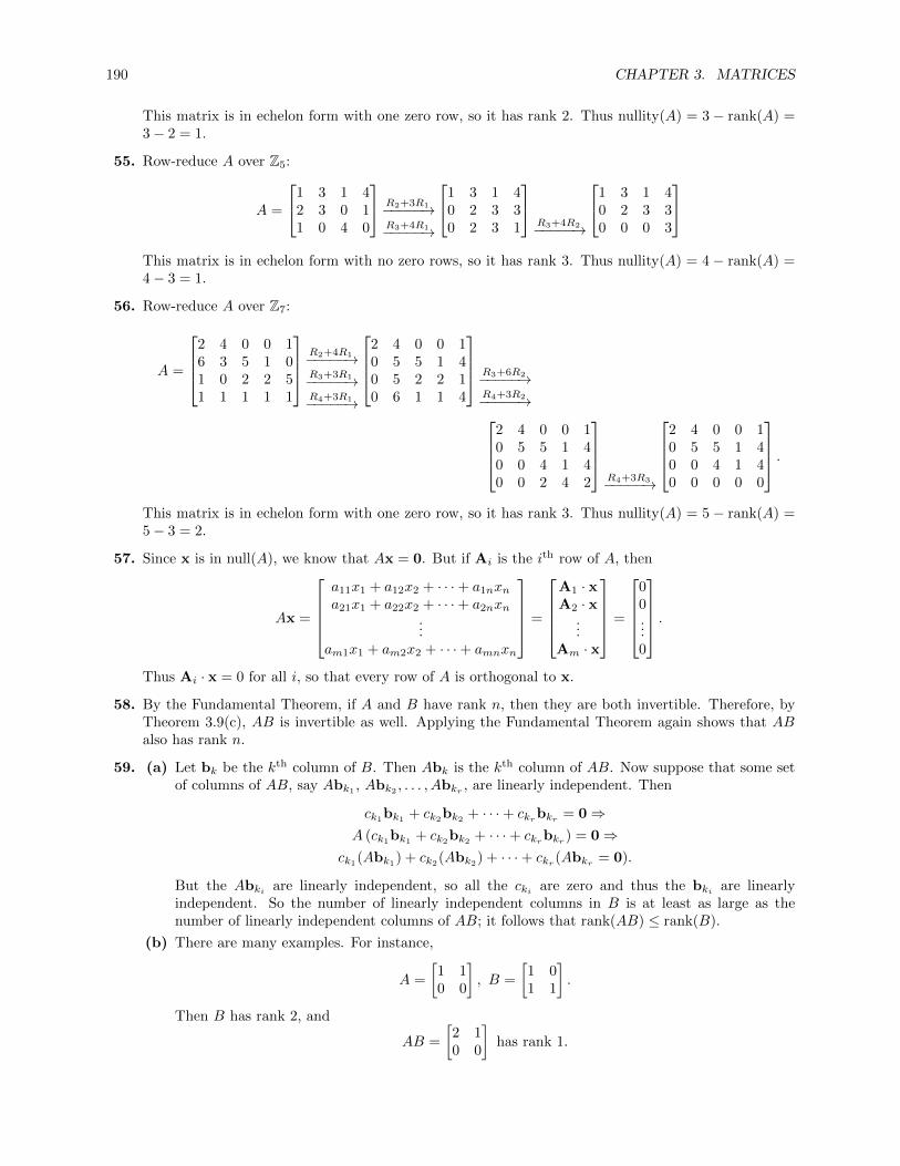
190 CHAPTER 3. MATRICES
This matrix is in echelon form with one zero row, so it has rank 2. Thus nullity(A) = 3 − rank(A) =3− 2 = 1.
55. Row-reduce A over Z5:
A =
1 3 1 42 3 0 11 0 4 0
R2+3R1−−−−−→R3+4R1−−−−−→
1 3 1 40 2 3 30 2 3 1
R3+4R2−−−−−→
1 3 1 40 2 3 30 0 0 3
This matrix is in echelon form with no zero rows, so it has rank 3. Thus nullity(A) = 4 − rank(A) =4− 3 = 1.
56. Row-reduce A over Z7:
A =
2 4 0 0 16 3 5 1 01 0 2 2 51 1 1 1 1
R2+4R1−−−−−→R3+3R1−−−−−→R4+3R1−−−−−→
2 4 0 0 10 5 5 1 40 5 2 2 10 6 1 1 4
R3+6R2−−−−−→R4+3R2−−−−−→
2 4 0 0 10 5 5 1 40 0 4 1 40 0 2 4 2
R4+3R3−−−−−→
2 4 0 0 10 5 5 1 40 0 4 1 40 0 0 0 0
.This matrix is in echelon form with one zero row, so it has rank 3. Thus nullity(A) = 5 − rank(A) =5− 3 = 2.
57. Since x is in null(A), we know that Ax = 0. But if Ai is the ith row of A, then
Ax =
a11x1 + a12x2 + · · ·+ a1nxna21x1 + a22x2 + · · ·+ a2nxn
...am1x1 + am2x2 + · · ·+ amnxn
=
A1 · xA2 · x
...Am · x
=
00...0
.Thus Ai · x = 0 for all i, so that every row of A is orthogonal to x.
58. By the Fundamental Theorem, if A and B have rank n, then they are both invertible. Therefore, byTheorem 3.9(c), AB is invertible as well. Applying the Fundamental Theorem again shows that ABalso has rank n.
59. (a) Let bk be the kth column of B. Then Abk is the kth column of AB. Now suppose that some setof columns of AB, say Abk1 , Abk2 , . . . , Abkr , are linearly independent. Then
ck1bk1 + ck2bk2 + · · ·+ ckrbkr = 0⇒A (ck1bk1 + ck2bk2 + · · ·+ ckrbkr ) = 0⇒
ck1(Abk1) + ck2(Abk2) + · · ·+ ckr (Abkr = 0).
But the Abki are linearly independent, so all the cki are zero and thus the bki are linearlyindependent. So the number of linearly independent columns in B is at least as large as thenumber of linearly independent columns of AB; it follows that rank(AB) ≤ rank(B).
(b) There are many examples. For instance,
A =
[1 10 0
], B =
[1 01 1
].
Then B has rank 2, and
AB =
[2 10 0
]has rank 1.
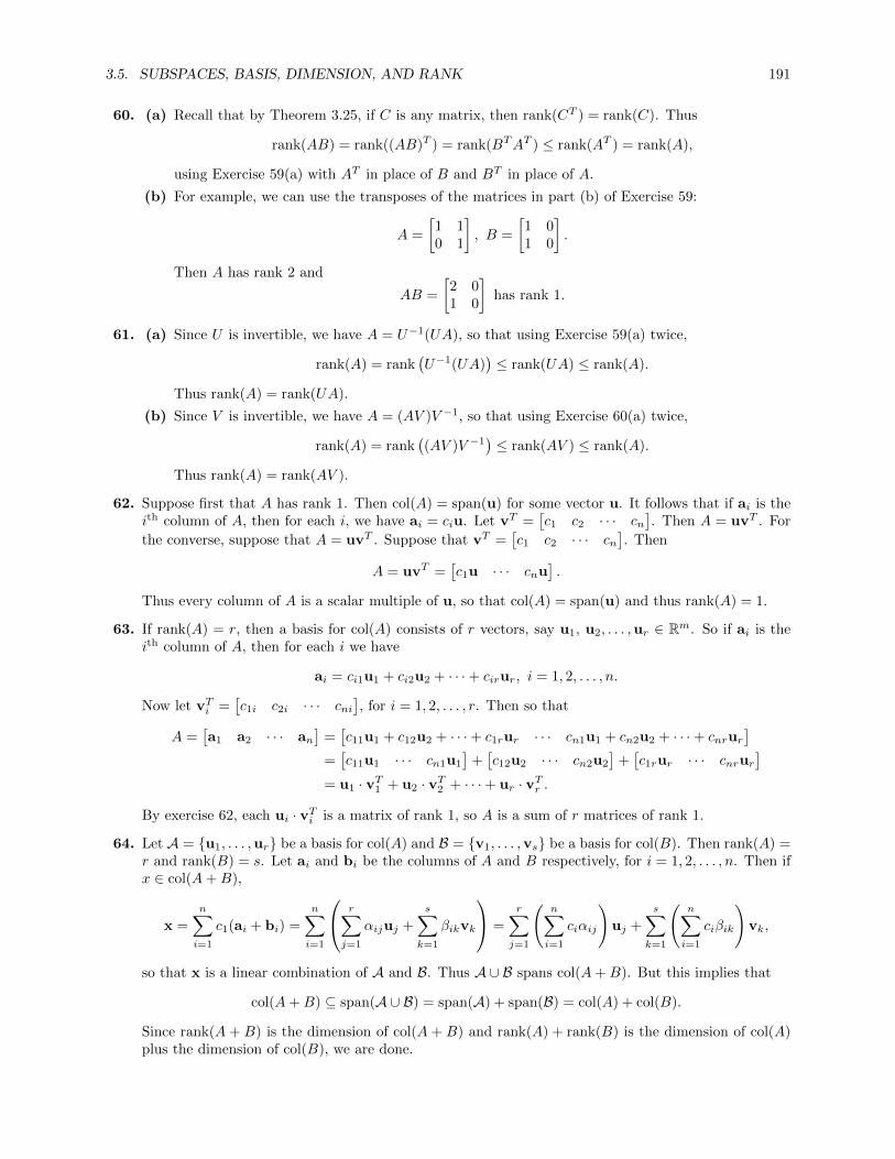
3.5. SUBSPACES, BASIS, DIMENSION, AND RANK 191
60. (a) Recall that by Theorem 3.25, if C is any matrix, then rank(CT ) = rank(C). Thus
rank(AB) = rank((AB)T ) = rank(BTAT ) ≤ rank(AT ) = rank(A),
using Exercise 59(a) with AT in place of B and BT in place of A.
(b) For example, we can use the transposes of the matrices in part (b) of Exercise 59:
A =
[1 10 1
], B =
[1 01 0
].
Then A has rank 2 and
AB =
[2 01 0
]has rank 1.
61. (a) Since U is invertible, we have A = U−1(UA), so that using Exercise 59(a) twice,
rank(A) = rank(U−1(UA)
)≤ rank(UA) ≤ rank(A).
Thus rank(A) = rank(UA).
(b) Since V is invertible, we have A = (AV )V −1, so that using Exercise 60(a) twice,
rank(A) = rank((AV )V −1
)≤ rank(AV ) ≤ rank(A).
Thus rank(A) = rank(AV ).
62. Suppose first that A has rank 1. Then col(A) = span(u) for some vector u. It follows that if ai is theith column of A, then for each i, we have ai = ciu. Let vT =
[c1 c2 · · · cn
]. Then A = uvT . For
the converse, suppose that A = uvT . Suppose that vT =[c1 c2 · · · cn
]. Then
A = uvT =[c1u · · · cnu
].
Thus every column of A is a scalar multiple of u, so that col(A) = span(u) and thus rank(A) = 1.
63. If rank(A) = r, then a basis for col(A) consists of r vectors, say u1, u2, . . . ,ur ∈ Rm. So if ai is theith column of A, then for each i we have
ai = ci1u1 + ci2u2 + · · ·+ cirur, i = 1, 2, . . . , n.
Now let vTi =[c1i c2i · · · cni
], for i = 1, 2, . . . , r. Then so that
A =[a1 a2 · · · an
]=[c11u1 + c12u2 + · · ·+ c1rur · · · cn1u1 + cn2u2 + · · ·+ cnrur
]=[c11u1 · · · cn1u1
]+[c12u2 · · · cn2u2
]+[c1rur · · · cnrur
]= u1 · vT1 + u2 · vT2 + · · ·+ ur · vTr .
By exercise 62, each ui · vTi is a matrix of rank 1, so A is a sum of r matrices of rank 1.
64. Let A = {u1, . . . ,ur} be a basis for col(A) and B = {v1, . . . ,vs} be a basis for col(B). Then rank(A) =r and rank(B) = s. Let ai and bi be the columns of A and B respectively, for i = 1, 2, . . . , n. Then ifx ∈ col(A+B),
x =
n∑i=1
c1(ai + bi) =
n∑i=1
r∑j=1
αijuj +
s∑k=1
βikvk
=
r∑j=1
(n∑i=1
ciαij
)uj +
s∑k=1
(n∑i=1
ciβik
)vk,
so that x is a linear combination of A and B. Thus A ∪ B spans col(A+B). But this implies that
col(A+B) ⊆ span(A ∪ B) = span(A) + span(B) = col(A) + col(B).
Since rank(A + B) is the dimension of col(A + B) and rank(A) + rank(B) is the dimension of col(A)plus the dimension of col(B), we are done.

192 CHAPTER 3. MATRICES
65. We show that col(A) ⊆ null(A) and then use the Rank Theorem. Suppose x =∑ciai ∈ col(A). Let
ai be the ith column of A; then ai = Aei where the ei are the standard basis vectors for Rn. Then
Ax = A(∑
ciai
)=∑
ci (Aai) =∑
ci (A (Aei)) =∑
ci(A2ei
)=∑
ci (Oei) = 0.
Thus any vector in the column space of A is taken to zero by A, so it is in the null space of A. Thuscol(A) ⊆ null(A). But then
rank(A) = dim(col(A)) ≤ dim(null(A)) = nullity(A),
so by the Rank Theorem,
rank(A) + rank(A) ≤ rank(A) + nullity(A) = n ⇒ 2 rank(A) ≤ n ⇒ rank(A) ≤ n
2.
66. (a) Note first that since x is n×1, then xT is 1×n and thus xTAx is 1×1. Thus(xTAx
)T= xTAx.
Now since A is skew-symmetric,
xTAx =(xTAx
)T= xTAT
(xT)T
= xT (−A)x = −xTAx.
So xTAx is equal to its own negation, so it must be zero.
(b) By Theorem 3.27, to show I + A is invertible it suffices to show that null(I + A) = 0. Choose xwith (I +A)x = 0. Then xT (I +A)x = xT0 = x · 0 = 0, so that
0 = xT (I +A)x = xT Ix + xTAx = xT Ix + xT0 = xT Ix = xTx = x · x
since Ax = 0. But x · x = 0 implies that x = 0. So any vector in null(I + A) is the zero vectorand thus I +A has a zero null space, so it is invertible.
3.6 Introduction to Linear Transformations
1. We must compute T (u) and T (v), so we take the product of the matrix A of T and each of these twovectors:
T (u) = Au =
[2 −13 4
] [12
]=
[011
]T (v) = Av =
[2 −13 4
] [12
]=
[81
].
2. We must compute T (u) and T (v), so we take the product of the matrix A of T and each of these twovectors:
T (u) = Au =
3 −11 21 4
[12
]=
3 · 1− 1 · 21 · 1 + 2 · 21 · 1 + 4 · 2
=
159
T (v) = Av =
3 −11 21 4
[ 3−2
]=
3 · 3− 1 · (−2)1 · 3 + 2 · (−2)1 · 3 + 4 · (−2)
=
11−1−5
3. Use the remark following Example 3.55. T is a linear transformation if and only if
T (c1v1 + c2v2) = c1T (v1) + c2T (v2), where v1 =
[x1
y1
], v2 =
[x2
y2
].

3.6. INTRODUCTION TO LINEAR TRANSFORMATIONS 193
Then
T (c1v1 + c2v2) = T
(c1
[x1
y1
]+ c2
[x2
y2
])= T
[c1x1 + c2x2
c1y1 + c2y2
]=
[(c1x1 + c2x2) + (c1y1 + c2y2)(c1x1 + c2x2)− (c1y1 + c2y2)
]=
[(c1x1 + c1y1) + (c2x2 + c2y2)(c1x1 − c1y1) + (c2x2 − c2y2)
]=
[c1x1 + c1y1
c1x1 − c1y1
]+
[c2x2 + c2y2
c2x2 − c2y2
]= c1
[x1 + y1
x1 − y1
]+ c2
[x2 + y2
x2 − y2
]= c1T (v1) + c2T (v2)
and thus T is linear.
4. Use the remark following Example 3.55. T is a linear transformation if and only if
T (c1v1 + c2v2) = c1T (v1) + c2T (v2), where v1 =
[x1
y1
], v2 =
[x2
y2
].
Then
T (c1v1 + c2v2) = T
(c1
[x1
y1
]+ c2
[x2
y2
])= T
[c1x1 + c2x2
c1y1 + c2y2
]
=
−(c1y1 + c2y2)(c1x1 + c2x2) + 2(c1y1 + c2y2)3(c1x1 + c2x2)− 4(c1y1 + c2y2)
=
−c1y1
c1x1 + 2c1y1
3c1x1 − 4c1y1
+
−c2y2
c2x2 + 2c2y2
3c2x2 − 4c2y2
= c1
−y1
x1 + 2y1
3x1 − 4y1
+ c2
−y2
x2 + 2y2
3x2 − 4y2
= c1T (v1) + c2T (v2)
and thus T is linear.
5. Use the remark following Example 3.55. T is a linear transformation if and only if
T (c1v1 + c2v2) = c1T (v1) + c2T (v2), where v1 =
x1
y1
z1
, v2 =
x2
y2
z2
.

194 CHAPTER 3. MATRICES
Then
T (c1v1 + c2v2) = T
c1x1
y1
z1
+ c2
x2
y2
z2
= T
c1x1 + c2x2
c1y1 + c2y2
c1z1 + c2z2
=
[(c1x1 + c2x2)− (c1y1 + c2y2) + (c1z1 + c2z2)
2(c1x1 + c2x2) + (c1y1 + c2y2)− 3(c1z1 + c2z2)
]=
[(c1x1 − c1y1 + c1z1) + (c2x2 − c2y2 + c2z2)
(2c1x1 + c1y1 − 3c1z1) + (2c2x2 + c2y2 − 3c2z2)
]=
[c1x1 − c1y1 + c1z1
2c1x1 + c1y1 − 3c1z1
]+
[c2x2 − c2y2 + c2z2
2c2x2 + c2y2 − 3c2z2
]= c1
[x1 − y1 + z1
2x1 + y1 − 3z1
]+ c2
[x2 − y2 + z2
2x2 + y2 − 3z2
]= c1T (v1) + c2T (v2)
and thus T is linear.
6. Use the remark following Example 3.55. T is a linear transformation if and only if
T (c1v1 + c2v2) = c1T (v1) + c2T (v2), where v1 =
x1
y1
z1
, v2 =
x2
y2
z2
.Then
T (c1v1 + c2v2) = T
c1x1
y1
z1
+ c2
x2
y2
z2
= T
c1x1 + c2x2
c1y1 + c2y2
c1z1 + c2z2
=
(c1x1 + c2x2) + (c1z1 + c2z2)(c1y1 + c2y2) + (c1z1 + c2z2)(c1x1 + c2x2) + (c1y1 + c2y2)
=
c1x1 + c1z1
c1y1 + c1z1
c1x1 + c1y1
+
c2x2 + c2z2
c2y2 + c2z2
c2x2 + c2y2
= c1
x1 + z1
y1 + z1
x1 + y1
+ c2
x2 + z2
y2 + z2
x2 + y2
= c1T (v1) + c2T (v2)
and thus T is linear.
7. For example,
T
[10
]=
[012
]=
[01
], T
[20
]=
[022
]=
[04
], but T
[1 + 2
0
]= T
[30
]=
[032
]=
[09
]6=[01
]+
[04
].
8. For example,
T
[−1
0
]=
[|−1||0|
]=
[10
], T
[10
]=
[|1||0|
]=
[10
], but T
[−1 + 1
0
]=
[00
]=
[|0||0|
]=
[00
]6=[10
]+
[10
].

3.6. INTRODUCTION TO LINEAR TRANSFORMATIONS 195
9. For example
T
[22
]=
[2 · 22 + 2
]=
[44
], but T
[2 + 22 + 2
]= T
[44
]=
[4 · 44 + 4
]=
[168
]6=[44
]+
[44
].
10. For example,
T
[10
]=
[1 + 10− 1
]=
[2−1
], but T
[1 + 10 + 0
]= T
[20
]=
[2 + 10− 1
]=
[3−1
]6=[
2−1
]+
[2−1
].
11. By Theorem 3.31, the standard matrix of T is the matrix A whose ith column is T (ei). Since
T (e1) = T
[10
]=
[1 + 01− 0
]=
[11
], T (e2) = T
[01
]=
[0 + 10− 1
]=
[1−1
],
the matrix of T is
A =
[1 11 −1
].
12. By Theorem 3.31, the standard matrix of T is the matrix A whose ith column is T (ei). Since
T (e1) = T
[10
]=
−01 + 2 · 0
3 · 1− 4 · 0
=
013
, T (e2) = T
[01
]=
−10 + 2 · 1
3 · 0− 4 · 1
=
−12−4
,the matrix of T is
A =
0 −11 23 −4
.13. By Theorem 3.31, the standard matrix of T is the matrix A whose ith column is T (ei). Since
T (e1) = T
100
=
[1− 0 + 0
2 · 1 + 0− 3 · 0
]=
[12
],
T (e2) = T
010
=
[0− 1 + 0
2 · 0 + 1− 3 · 0
]=
[−1
1
],
T (e3) = T
001
=
[0− 0 + 1
2 · 0 + 0− 3 · 1
]=
[1−3
],
the matrix of T is
A =
[1 −1 12 1 −3
].
14. By Theorem 3.31, the standard matrix of T is the matrix A whose ith column is T (ei). Since
T (e1) = T
100
=
1 + 00 + 01 + 0
=
101
,T (e2) = T
010
=
0 + 01 + 00 + 1
=
011
,T (e3) = T
001
=
0 + 10 + 10 + 0
=
110
,

196 CHAPTER 3. MATRICES
the matrix of T is
A =
1 0 10 1 11 1 0
.15. Reflecting a vector in the x-axis means negating the x-coordinate. So using the method of Example
3.56,
F
[xy
]=
[−xy
]= x
[−1
0
]+ y
[01
],
and thus F is a matrix transformation with matrix
F =
[−1 0
0 1
].
It follows that F is a linear transformation.
16. Example 3.58 shows that a rotation of 45◦ about the origin sends[1
0
]to
[cos 45◦
sin 45◦
]=
[√2
2√2
2
]and
[0
1
]to
[cos 135◦
sin 135◦
]=
[−√
22√2
2
],
so that R is a matrix transformation with matrix
R =
[√2
2 −√
22√
22
√2
2
].
It follows that R is a linear transformation.
17. Since D stretches by a factor of 2 in the x-direction and a factor of 3 in the y-direction, we see that
D
[xy
]=
[2x3y
]=
[2 00 3
] [xy
].
Thus D is a matrix transformation with matrix[2 00 3
].
It follows that D is a linear transformation.
18. Since P = (x, y) projects onto the line whose direction vector is 〈1, 1〉, it follows that the projection ofP onto that line is
proj〈1,1〉 〈x, y〉 =
(〈x, y〉 · 〈1, 1〉〈1, 1〉 · 〈1, 1〉
)〈1, 1〉 =
⟨x+ y
2,x+ y
2
⟩.
Thus
T
[x
y
]=
[x+y
2x+y
2
]= x
[1212
]+ y
[1212
]=
[12
12
12
12
][x
y
].
Thus T is a matrix transformation with the matrix above, and it follows that T is a linear transforma-tion.
19. Let
A1 =
[k 00 1
], A2 =
[1 00 k
], B =
[0 11 0
], C1 =
[1 k0 1
], C2 =
[1 0k 1
]

3.6. INTRODUCTION TO LINEAR TRANSFORMATIONS 197
Then
A1
[xy
]=
[k 00 1
] [xy
]=
[kxy
]: A1 stretches vectors horizontally by a factor of k
A2
[xy
]=
[1 00 k
] [xy
]=
[xky
]: A2 stretches vectors vertically by a factor of k
B
[xy
]=
[0 11 0
] [xy
]=
[yx
]: B reflects vectors in the line y = x
C1
[xy
]=
[1 k0 1
] [xy
]=
[x+ kyy
]: C1 extends vectors horizontally by ky
C2
[xy
]=
[1 0k 1
] [xy
]=
[x
y + kx
]: C1 extends vectors vertically by kx
(C1 and C2 are called shears.) The effect of each of these transformations, with k = 2, on the unitsquare is
0 1 2 30
1
2
3
Original
0 1 2 30
1
2
3A1
0 1 2 30
1
2
3A2
0 1 2 30
1
2
3B
0 1 2 30
1
2
3C1
0 1 2 30
1
2
3C2
Note that reflection across the line y = x leaves the square unchanged, since it is symmetric about thatline.
20. Using the formula from Example 3.58, we compute the matrix for a counterclockwise rotation of 120◦:
R120◦(e1) =
[cos 120◦
sin 120◦
]=
[− 1
2√3
2
]and R120◦(e2) =
[− sin 120◦
cos 120◦
]=
[−√
32
− 12
].
So by Theorem 3.31, we have
A =[R120◦(e1) R120◦(e2)
]=
[− 1
2 −√
32√
32
12
].

198 CHAPTER 3. MATRICES
21. A clockwise rotation of 30◦ is a rotation of −30◦. Then using the formula from Example 3.58, wecompute the matrix for that rotation:
R−30◦(e1) =
[cos(−30◦)
sin(−30◦)
]=
[√3
2
− 12
]and R120◦(e2) =
[− sin(−30◦)
cos(−30◦)
]=
[12√3
2
].
So by Theorem 3.31, we have
A =[R−30◦(e1) R−30◦(e2)
]=
[√3
212
− 12
√3
2
].
22. A direction vector of the line y = 2x is d =
[12
], so
P`(e1) =
(d · e1
d · d
)d =
1
1 + 4
[1
2
]=
[1525
]and P`(e2) =
(d · e2
d · d
)d =
2
1 + 4
[1
2
]=
[2545
].
Thus by Theorem 3.31, we have
A =[P`(e1) P`(e2)
]=
[15
25
25
45
].
23. A direction vector of the line y = −x is d =
[1−1
], so
P`(e1) =
(d · e1
d · d
)d =
1
1 + 1
[1
−1
]=
[12
− 12
]and P`(e2) =
(d · e2
d · d
)d =
−1
1 + 2
[1
−1
]=
[− 1
212
].
Thus by Theorem 3.31, we have
A =[P`(e1) P`(e2)
]=
[12 − 1
2
− 12
12
].
24. Reflection in the line y = x is given by
R
[xy
]=
[yx
]= x
[01
]+ y
[10
]=
[0 11 0
] [xy
],
so that the matrix of R is [0 11 0
].
25. Reflection in the line y = −x is given by
R
[xy
]=
[−y−x
]= x
[0−1
]+ y
[−1
0
]=
[0 −1−1 0
] [xy
],
so that the matrix of R is [0 −1−1 0
].
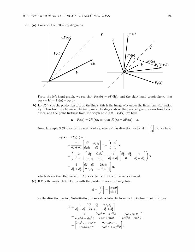
3.6. INTRODUCTION TO LINEAR TRANSFORMATIONS 199
26. (a) Consider the following diagrams:
b
F{HbL
cb
c F{HbL{
a
b
a + b
F{Ha + bL
F{HaL
F{HaL
F{HbL
{
From the left-hand graph, we see that F`(cb) = cF`(b), and the right-hand graph shows thatF`(a + b) = F`(a) + F`(b).
(b) Let P`(x) be the projection of x on the line `; this is the image of x under the linear transformationP`. Then from the figure in the text, since the diagonals of the parallelogram shown bisect eachother, and the point furthest from the origin on ` is x + F`(x), we have
x + F`(x) = 2P`(x), so that F`(x) = 2P`(x)− x.
Now, Example 3.59 gives us the matrix of P`, where ` has direction vector d =
[d1
d2
], so we have
F`(x) = 2P`(x)− x
=2
d21 + d2
2
[d2
1 d1d2
d1d2 d22
]x−
[1 0
0 1
]x
=
(2
d21 + d2
2
[d2
1 d1d2
d1d2 d22
]− 1
d21 + d2
2
[d2
1 + d22 0
0 d21 + d2
2
])x
=1
d21 + d2
2
[d2
1 − d22 2d1d2
2d1d2 −d21 + d2
2
]x,
which shows that the matrix of F` is as claimed in the exercise statement.
(c) If θ is the angle that ` forms with the positive x-axis, we may take
d =
[d1
d2
]=
[cos θsin θ
]as the direction vector. Substituting those values into the formula for F` from part (b) gives
F` =1
d21 + d2
2
[d2
1 − d22 2d1d2
2d1d2 −d21 + d2
2
]=
1
cos2 θ + sin2 θ
[cos2 θ − sin2 θ 2 cos θ sin θ
2 cos θ sin θ − cos2 θ + sin2 θ
]=
[cos2 θ − sin2 θ 2 cos θ sin θ
2 cos θ sin θ − cos2 θ + sin2 θ
],

200 CHAPTER 3. MATRICES
since cos2 θ + sin2 θ = 1. Now, cos2 θ − sin2 θ = cos 2θ, and 2 cos θ sin θ = sin 2θ, so the matrixabove simplifies to
F` =
[cos 2θ sin 2θsin 2θ − cos 2θ
].
27. By part (b) of the previous exercise, since the line y = 2x has direction vector d =
[12
], we have for
the standard matrix of this reflection
F`(x) =1
1 + 4
[1− 4 2 · 22 · 2 −1 + 4
]=
[− 3
545
45
35
].
28. The direction vector of this line is
[1√3
], so that sin θ
cos θ =√
31 =
√3, and thus θ = π
3 = 60◦. So by part
(c) of the previous exercise, the standard matrix of this reflection is
F`(x) =
[cos 2θ sin 2θ
sin 2θ − cos 2θ
]=
[cos 120◦ sin 120◦
sin 120◦ − cos 120◦
]=
[−√
32
12
12
√3
2
].
29. Since
T
[x1
x2
]=
x1
2x1 − x2
3x1 + 4x2
, S
y1
y2
y3
=
2y1 + y3
3y2 − y3
y1 − y2
y1 + y2 + y3
,we substitute the result of T into the equation for S:
(S ◦ T )
[x1
x2
]= S
x1
2x1 − x2
3x1 + 4x2
=
2x1 + (3x1 + 4x2)
3(2x1 − x2)− (3x1 + 4x2)x1 − (2x1 − x2)
x1 + (2x1 − x2) + (3x1 + 4x2)
=
5x1 + 4x2
3x1 − 7x2
−x1 + x2
6x1 + 3x2
=
5 43 −7−1 1
6 3
[x1
x2
].
Thus the standard matrix of S ◦ T is
A =
5 43 −7−1 1
6 3
.30. (a) By direct substitution, we have
(S ◦ T )
[x1
x2
]= S
(T
[x1
x2
])= S
[x1 − x2
x1 + x2
]=
[2(x1 − x2)−(x1 + x2)
]=
[2x1 − 2x2
−x1 − x2
].
Thus
[S ◦ T ] =
[2 −2−1 −1
].

3.6. INTRODUCTION TO LINEAR TRANSFORMATIONS 201
(b) Using matrix multiplication, we first find the standard matrices for S and T , which are
[S] =
[2 00 −1
], [T ] =
[1 −11 1
].
Then
[S][T ] =
[2 00 −1
] [1 −11 1
]=
[2 −2−1 −1
].
Then [S ◦ T ] = [S][T ].
31. (a) By direct substitution, we have
(S ◦ T )
[x1
x2
]= S
(T
[x1
x2
])= S
[x1 + 2x2
−3x1 + x2
]=
[(x1 + 2x2) + 3(−3x1 + x2)(x1 + 2x2)− (−3x1 + x2)
]=
[−8x1 + 5x2
4x1 + x1
].
Thus
[S ◦ T ] =
[−8 5
4 1
].
(b) Using matrix multiplication, we first find the standard matrices for S and T , which are
[S] =
[1 31 −1
], [T ] =
[1 2−3 1
].
Then
[S][T ] =
[1 31 −1
] [1 2−3 1
]=
[−8 5
4 1
].
Then [S ◦ T ] = [S][T ].
32. (a) By direct substitution, we have
(S ◦ T )
[x1
x2
]= S
(T
[x1
x2
])= S
[x2
−x1
]=
x2 + 3(−x1)2x2 − x1
x2 − (−x1)
=
−3x1 + x2
−x1 + 2x2
x1 + x2
.Thus
[S ◦ T ] =
−3 1−1 2
1 1
.(b) Using matrix multiplication, we first find the standard matrices for S and T , which are
[S] =
1 32 11 −1
, [T ] =
[0 1−1 0
].
Then
[S][T ] =
1 32 11 −1
[ 0 1−1 0
]=
−3 1−1 2
1 1
.Then [S ◦ T ] = [S][T ].
33. (a) By direct substitution, we have
(S ◦ T )
x1
x2
x3
= S
Tx1
x2
x3
= S
[x1 + x2 − x3
2x1 − x2 + x3
]
=
[4(x1 + x2 − x3)− 2(2x1 − x2 + x3)−(x1 + x2 − x3) + (2x1 − x2 + x3)
]=
[6x2 − 6x3
x1 − 2x2 + 2x3
]
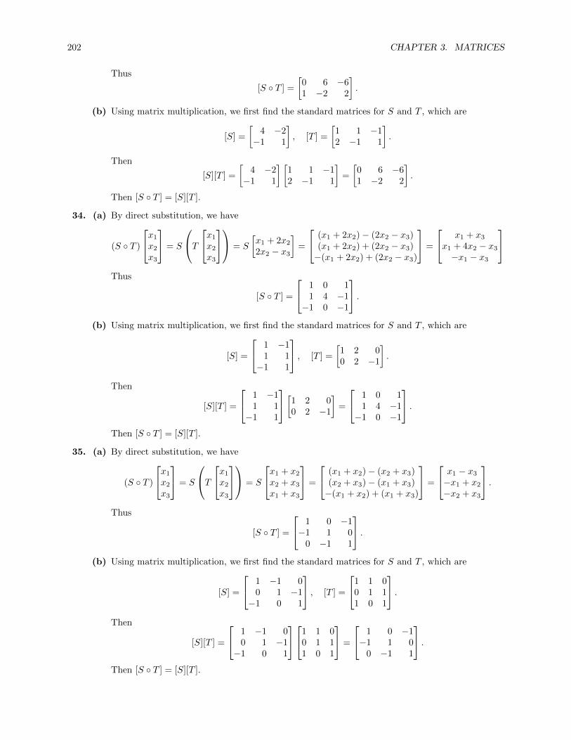
202 CHAPTER 3. MATRICES
Thus
[S ◦ T ] =
[0 6 −61 −2 2
].
(b) Using matrix multiplication, we first find the standard matrices for S and T , which are
[S] =
[4 −2−1 1
], [T ] =
[1 1 −12 −1 1
].
Then
[S][T ] =
[4 −2−1 1
] [1 1 −12 −1 1
]=
[0 6 −61 −2 2
].
Then [S ◦ T ] = [S][T ].
34. (a) By direct substitution, we have
(S ◦ T )
x1
x2
x3
= S
Tx1
x2
x3
= S
[x1 + 2x2
2x2 − x3
]=
(x1 + 2x2)− (2x2 − x3)(x1 + 2x2) + (2x2 − x3)−(x1 + 2x2) + (2x2 − x3)
=
x1 + x3
x1 + 4x2 − x3
−x1 − x3
Thus
[S ◦ T ] =
1 0 11 4 −1−1 0 −1
.(b) Using matrix multiplication, we first find the standard matrices for S and T , which are
[S] =
1 −11 1−1 1
, [T ] =
[1 2 00 2 −1
].
Then
[S][T ] =
1 −11 1−1 1
[1 2 00 2 −1
]=
1 0 11 4 −1−1 0 −1
.Then [S ◦ T ] = [S][T ].
35. (a) By direct substitution, we have
(S ◦ T )
x1
x2
x3
= S
Tx1
x2
x3
= S
x1 + x2
x2 + x3
x1 + x3
=
(x1 + x2)− (x2 + x3)(x2 + x3)− (x1 + x3)−(x1 + x2) + (x1 + x3)
=
x1 − x3
−x1 + x2
−x2 + x3
.Thus
[S ◦ T ] =
1 0 −1−1 1 0
0 −1 1
.(b) Using matrix multiplication, we first find the standard matrices for S and T , which are
[S] =
1 −1 00 1 −1−1 0 1
, [T ] =
1 1 00 1 11 0 1
.Then
[S][T ] =
1 −1 00 1 −1−1 0 1
1 1 00 1 11 0 1
=
1 0 −1−1 1 0
0 −1 1
.Then [S ◦ T ] = [S][T ].

3.6. INTRODUCTION TO LINEAR TRANSFORMATIONS 203
36. A counterclockwise rotation T through 60◦ is given by (see Example 3.58)
[T ] =
[cos 60◦ − sin 60◦
sin 60◦ cos 60◦
]=
[12 −
√3
2√3
212
],
and reflection S in y = x is reflection in a line with direction vector d =
[11
], which has the matrix
(see Exercise 26(b))
[S] =1
2
[0 22 0
]=
[0 11 0
].
Thus by Theorem 3.32, the composite transformation is given by
[S ◦ T ] = [S][T ] =
[0 1
1 0
][12 −
√3
2√3
212
]=
[√3
212
12 −
√3
2
].
37. Reflection T in the y-axis is taking the negative of the x-coordinate, so it has matrix
[T ] =
[−1 0
0 1
],
while clockwise rotation S through 30◦ has matrix (see Example 3.58)
[S] =
[cos(−30◦) − sin(−30◦)
sin(−30◦) cos(−30◦)
]=
[√3
212
− 12
√3
2
].
Thus by Theorem 3.32, the composite transformation is given by
[S ◦ T ] = [S][T ] =
[√3
212
− 12
√3
2
][−1 0
0 1
]=
[−√
32
12
12
√3
2
].
38. Clockwise rotation T through 45◦ has matrix (see Example 3.58)
[T ] =
[cos 45◦ sin 45◦
− sin 45◦ cos 45◦
]=
[ √2
2
√2
2
−√
22
√2
2
],
while projection S onto the y-axis has matrix (see Example 3.59, or note that this transformationsimply sets the x-coordinate to zero)
[S] =
[0 00 1
].
Thus by Theorem 3.32, the composite transformation is given by
[T ◦ S ◦ T ] = [T ][S][T ] =
[ √2
2
√2
2
−√
22
√2
2
][0 0
0 1
][ √2
2
√2
2
−√
22
√2
2
]=
[− 1
212
− 12
12
].
39. Reflection T in the line y = x, with direction vector d =
[11
], is given by (see Exercise 26(b))
[T ] =1
2
[0 22 0
]=
[0 11 0
].
Counterclockwise rotation S through 30◦ has matrix (see Example 3.58)
[S] =
[cos 30◦ sin 30◦
− sin 30◦ cos 30◦
]=
[ √3
212
− 12
√3
2
].

204 CHAPTER 3. MATRICES
Finally, reflection R in the line y = −x, with direction vector d =
[1−1
], is given by (see Exercise
26(b))
[R] =1
2
[0 −2−2 0
]=
[0 −1−1 0
].
Then by Theorem 3.32, the composite transformation is given by
[R ◦ S ◦ T ] = [R][S][T ] =
[0 −1
−1 0
][ √3
212
− 12
√3
2
][0 1
1 0
]=
[−√
32 − 1
212 −
√3
2
].
40. Using the formula for rotation through an angle θ, from Example 3.58, we have
[Rα ◦Rβ ] = [Rα][Rβ ] =
[cosα − sinαsinα cosα
] [cosβ − sinβsinβ cosβ
]=
[cosα cosβ − sinα sinβ − cosα sinβ − sinα cosβsinα cosβ + cosα sinβ − sinα sinβ + cosα cosβ
]=
[cos(α+ β) − sin(α+ β)sin(α+ β) cos(α+ β)
]= Rα+β .
41. Assume line ` has direction vector l =
[cosαsinα
]and line m has direction vector
[cosβsinβ
]. Let θ = β − α
be the angle from ` to m (note that if α > β, then θ is negative). Then by Exercise 26(c),
Fm ◦ F` =
[cos 2β sin 2βsin 2β − cos 2β
] [cos 2α sin 2αsin 2α − cos 2α
]=
[cos 2β cos 2α+ sin 2β sin 2α cos 2β sin 2α− sin 2β cos 2αsin 2β cos 2α− cos 2β sin 2α cos 2β cos 2α+ sin 2β sin 2α
]=
[cos(2(α− β)) sin(2(α− β))− sin(2(α− β)) cos(2(α− β))
]=
[cos(2(β − α)) − sin(2(β − α))sin(2(β − α)) cos(2(β − α))
]=
[cos 2θ − sin 2θsin 2θ cos 2θ
]= R2θ.
42. (a) Let P be the projection onto a line with direction vector d =
[d1
d2
]. Then the standard matrix of
P is
P =1
d21 + d2
2
[d2
1 d1d2
d1d2 d22
],
and thus
P ◦ P = P 2 =1
d21 + d2
2
[d2
1 d1d2
d1d2 d22
]1
d21 + d2
2
[d2
1 d1d2
d1d2 d22
]=
1
(d21 + d2
2)2
[d4
1 + d21d
22 d3
1d2 + d1d32
d31d2 + d1d
32 d2
1d22 + d4
2
]=
1
(d21 + d2
2)2
[d2
1(d21 + d2
2) d1d2(d21 + d2
2)d1d2(d2
1 + d22) d2
2(d21 + d2
2)
]=
1
d21 + d2
2
[d2
1 d1d2
d1d2 d22
]= P.

3.6. INTRODUCTION TO LINEAR TRANSFORMATIONS 205
Note that we have proven this fact before, in a different form. Since P (v) = projd v, then
(P ◦ P )(v) = projd(projd v) = projd v = P (v)
by Exercise 70(a) in Section 1.2.
(b) Let P be any projection matrix. Using the form of P from the previous exercise, we first provethat P 6= I. Suppose it were. Then d1d2 = 0, so that either d1 = 0 or d2 = 0. But then either d2
1
or d22 would be zero, so that P could not be the identity matrix. So P is a non-identity matrix
such that P 2 = P . Then P 2 − P = P (P − I) = O. Since P 6= I, we see that P − I 6= O, sothere is some k such that (P − I)ek 6= 0 (otherwise, every row of P − I would be orthogonalto every standard basis vector, so would be zero, so that P − I would be the zero matrix). Letx = (P − I)ek. But then
Px = P (P − I)ek = Oek = 0,
so that x ∈ null(P ). Since the null space of P contains a nonzero vector, P is not invertible byTheorem 3.27.
43. Let `, m, and n be lines through the origin with angles from the x-axis of θ, α, and β respectively.Then
Fn ◦ Fm ◦ F` =
[cos 2θ sin 2θsin 2θ − cos 2θ
] [cos 2α sin 2αsin 2α − cos 2α
] [cos 2β sin 2βsin 2β − cos 2β
]=
[cos 2θ cos 2α+ sin 2θ sin 2α cos 2θ sin 2α− sin 2θ cos 2αsin 2θ cos 2α− cos 2θ sin 2α sin 2θ sin 2α+ cos 2θ cos 2α
] [cos 2β sin 2βsin 2β − cos 2β
]=
[cos 2(θ − α) − sin 2(θ − α)sin 2(θ − α) cos 2(θ − α)
] [cos 2β sin 2βsin 2β − cos 2β
]=
[cos 2(θ − α) cos 2β − sin 2(θ − α) sin 2β cos 2(θ − α) sin 2β + sin 2(θ − α) cos 2βsin 2(θ − α) cos 2β + cos 2(θ − α) sin 2β sin 2(θ − α) sin 2β − cos 2(θ − α) cos 2β
]=
[cos 2(θ − α+ β) sin 2(θ − α+ β)sin 2(θ − α+ β) − cos 2(θ − α+ β)
].
This is a reflection through a line making an angle of θ − α+ β with the x-axis.
44. If ` is a line with direction vector d through the point P , then it has equation x = p + td. Since T islinear, we have
T (x) = T (p + td) = T (p) + tT (d),
so that the equation of the resulting graph has equation T (x) = T (p) + tT (d). If T (d) = 0, then theimage of ` has equation T (x) = T (p) so that it is the single point T (p). Otherwise, the image of ` isthe line `′ with direction vector T (d) passing through T (p).
45. Suppose that we start with two parallel lines
` : x = p + td, m : x = q + sd.
Then the images of these lines have equations
`′ : T (p) + tT (d), m′ : T (q) + sT (d).
Then
• If T (d) 6= 0 and T (p) 6= T (q), then `′ and m′ are distinct parallel lines.
• If T (d) 6= 0 and T (p) = T (q), then `′ and m′ are the same line.
• If T (d) = 0 and T (p) 6= T (q), then `′ and m′ are distinct points T (p) and T (q).
• If T (d) = 0 and T (p) 6= T (q), then `′ and m′ are the single point T (p).

206 CHAPTER 3. MATRICES
46. Using the linear transformation T from Exercise 3, we have
T
[−1
1
]=
[0−2
], T
[11
]=
[20
], T
[1−1
]=
[02
], T
[−1−1
]=
[−2
0
].
The image is the square below:
A
B
C
D
-2 -1 1 2
-2
-1
1
2
47. Using the linear transformation D from Exercise 17, we have
D
[−1
1
]=
[−2
3
], D
[11
]=
[23
], D
[1−1
]=
[2−3
], D
[−1−1
]=
[−2−3
].
The image is the rectangle below:
A B
CD
-2 -1 1 2
-2
-1
1
2
3
48. Using the linear transformation P from Exercise 18, we have
P
[−1
1
]=
[00
], P
[11
]=
[11
], P
[1−1
]=
[00
], P
[−1−1
]=
[−1−1
].
The image is the line below:

3.6. INTRODUCTION TO LINEAR TRANSFORMATIONS 207
A
B
C
D
-1. -0.5 0.5 1.
-1.
-0.5
0.5
1.
49. Using the projection P from Exercise 22, we have
P
[−1
1
]=
[1525
], P
[1
1
]=
[3565
], P
[1
−1
]=
[− 1
5
− 25
], P
[−1
−1
]=
[− 3
5
− 65
].
The image is the line below:
A
B
C
D
-1. -0.5 0.5 1.
-1.
-0.5
0.5
1.
50. Using the transformation T from Exercise 31, with matrix
[1 2−3 1
], we have
T
[−1
1
]=
[14
], T
[11
]=
[3−2
], T
[1−1
]=
[−1−4
], T
[−1−1
]=
[−3
2
].
The image is the parallelogram below:
A
B
C
D
-4 -3 -2 -1 1 2 3 4
-4
-3
-2
-1
1
2
3
4
51. Using the transformation resulting from Exercise 37, which we call Q, we have
Q
[−1
1
]=
[√3+12√3+12
], Q
[1
1
]=
[−√
3+12√3−12
], Q
[1
−1
]=
[−√
3−12
−√
3−12
], Q
[−1
−1
]=
[ √3−12
−√
3+12
].
The image is the parallelogram below:

208 CHAPTER 3. MATRICES
A
B
C
D
-1 1
-1
1
52. If ` has direction vector d, then using standard properties of the dot product and of scalar multiplica-tion, we get
P`(cv) = projd(cv) =
(d · cvd · d
)d =
(c(d · v)
d · d
)d = c
((d · vd · d
)d
)= cP`(v).
53. First suppose that T is linear. Then applying property 1 first, followed by property 2, we have
T (c1v1 + c2v2) = T (c1v1) + T (c2v2) = c1T (v1) + c2T (v2).
For the reverse direction, assume that T (c1v1 + c2v2) = c1T (v1) + c2T (v2). To prove property 1, setc1 = c2 = 1; this gives
T (v1 + v2) = T (v1) + T (v2).
For property 2, set c1 = c, v1 = v, and c2 = 0; this gives
T (cv) = T (cv + 0v2) = cT (v) + 0T (v2) = cT (v).
Thus T is linear.
54. Let range(T ) be the range of T and col([T ]) be the column space of [T ]. We show that range(T ) =col([T ]) by showing that they are both equal to span({T (ei)}).To see that range(T ) = span({T (ei)}), note that x ∈ range(T ) if and only if x = T (v) for somev =
∑ciei, so that
x = T (v) = T (∑
ciei) =∑
ciT (ei),
which is the case if and only if x ∈ span({T (ei)}). Thus range(T ) = span({T (ei)}).Next, we show that col([T ]) = span({T (ei)}). By Theorem 2, [T ] =
[T (e1) T (e2) · · · T (en)
].
Thus if vT =[v1 v2 · · · vn
], then
T (v) = v1T (e1) + v2T (e2) + · · ·+ vnT (en).
Then
x ∈ col([T ]) ⇐⇒ x = T (v) = T (∑
viT (ei)) =∑
viT (ei),
so that col([T ]) = span({T (ei)}).
55. The Fundamental Theorem of Invertible Matrices implies that any invertible 2× 2 matrix is a productof elementary matrices. The matrices in Exercise 19 represent the three types of elementary 2 × 2matrices, so TA must be a composition of the three types of transformations represented in Exercise19.

3.7. APPLICATIONS 209
3.7 Applications
1. x1 = Px0 =
[0.5 0.30.5 0.7
] [0.50.5
]=
[0.40.6
], x2 = Px1 =
[0.5 0.30.5 0.7
] [0.40.6
]=
[0.380.62
].
2. Since there are two steps involved, the proportion we seek will be [P 2]21 — the probability of a state1 population member being in state 2 after two steps:
P 2 =
[0.5 0.30.5 0.7
]2
=
[0.4 0.360.6 0.64
].
The proportion of the state 1 population in state 2 after two steps is 0.6.
3. Since there are two steps involved, the proportion we seek will be [P 2]22 — the probability of a state2 population member remaining in state 2 after two steps:
P 2 =
[0.5 0.30.5 0.7
]2
=
[0.4 0.360.6 0.64
].
The proportion of the state 2 population in state 2 after two steps is 0.64.
4. The steady-state vector x =
[x1
x2
]has the property that Px = x, or (I − P )x = 0. So we form the
augmented matrix of that system and row-reduce it:
[I − P 0
]:
[1− 0.5 −0.3 0−0.5 1− 0.7 0
]=
[0.5 −0.3 00.5 0.3 0
]→[1 −0.6 00 0 0
]Thus x2 = t is free and x1 = 3
5 t. Since we also want x to be a probability vector, we also havex1 + x2 = 3
5 t+ t = 85 t = 1, so that t = 5
8 . Thus the steady-state vector is
x =
[3858
].
5. x1 = Px0 =
12
13
13
0 13
23
12
13 0
120
180
90
=
150
120
120
, x2 = Px1 =
12
13
13
0 13
23
12
13 0
150
120
120
=
155
120
115
.6. Since there are two steps involved, the proportion we seek will be [P 2]11 — the probability of a state
1 population member being in state 1 after two steps:
P 2 =
12
13
13
0 13
23
12
13 0
2
=
512
718
718
13
13
29
14
518
718
.The proportion of the state 1 population in state 1 after two steps is 5
12 .
7. Since there are two steps involved, the proportion we seek will be [P 2]32 — the probability of a state2 population member being in state 3 after two steps:
P 2 =
12
13
13
0 13
23
12
13 0
2
=
512
718
718
13
13
29
14
518
718
.The proportion of the state 2 population in state 3 after two steps is 5
18 .
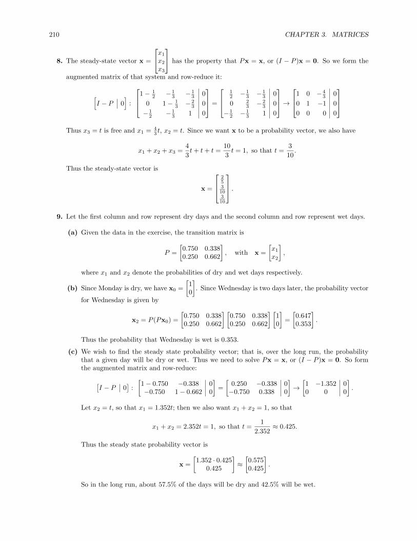
210 CHAPTER 3. MATRICES
8. The steady-state vector x =
x1
x2
x3
has the property that Px = x, or (I − P )x = 0. So we form the
augmented matrix of that system and row-reduce it:
[I − P 0
]:
1− 12 − 1
3 − 13 0
0 1− 13 − 2
3 0
− 12 − 1
3 1 0
=
12 − 1
3 − 13 0
0 23 − 2
3 0
− 12 − 1
3 1 0
→1 0 − 4
3 0
0 1 −1 0
0 0 0 0
Thus x3 = t is free and x1 = 4
3 t, x2 = t. Since we want x to be a probability vector, we also have
x1 + x2 + x3 =4
3t+ t+ t =
10
3t = 1, so that t =
3
10.
Thus the steady-state vector is
x =
25310310
.9. Let the first column and row represent dry days and the second column and row represent wet days.
(a) Given the data in the exercise, the transition matrix is
P =
[0.750 0.3380.250 0.662
], with x =
[x1
x2
],
where x1 and x2 denote the probabilities of dry and wet days respectively.
(b) Since Monday is dry, we have x0 =
[10
]. Since Wednesday is two days later, the probability vector
for Wednesday is given by
x2 = P (Px0) =
[0.750 0.3380.250 0.662
] [0.750 0.3380.250 0.662
] [10
]=
[0.6470.353
].
Thus the probability that Wednesday is wet is 0.353.
(c) We wish to find the steady state probability vector; that is, over the long run, the probabilitythat a given day will be dry or wet. Thus we need to solve Px = x, or (I − P )x = 0. So formthe augmented matrix and row-reduce:
[I − P 0
]:
[1− 0.750 −0.338 0−0.750 1− 0.662 0
]=
[0.250 −0.338 0−0.750 0.338 0
]→[1 −1.352 00 0 0
].
Let x2 = t, so that x1 = 1.352t; then we also want x1 + x2 = 1, so that
x1 + x2 = 2.352t = 1, so that t =1
2.352≈ 0.425.
Thus the steady state probability vector is
x =
[1.352 · 0.425
0.425
]≈[0.5750.425
].
So in the long run, about 57.5% of the days will be dry and 42.5% will be wet.

3.7. APPLICATIONS 211
10. Let the three rows (and columns) correspond to, in order, tall, medium, or short.
(a) From the given data, the transition matrix is
P =
0.6 0.1 0.20.2 0.7 0.40.2 0.2 0.4
.
(b) Starting with a short person, we have x0 =
001
. That person’s grandchild is two generations
later, so that
x2 = P (Px0) =
0.6 0.1 0.20.2 0.7 0.40.2 0.2 0.4
0.6 0.1 0.20.2 0.7 0.40.2 0.2 0.4
001
=
0.240.480.28
.So the probability that a grandchild will be tall is 0.24.
(c) The current distribution of heights is x0 =
0.20.50.3
, and we want to find x3:
x2 = P 3x0 =
0.6 0.1 0.20.2 0.7 0.40.2 0.2 0.4
3 0.20.50.3
=
0.24570.50390.2504
.So roughly 24.6% of the population is tall, 50.4% medium, and 25.0% short.
(d) We want to solve (I − P )x = 0, so form the augmented matrix and row-reduce:
[I − P 0
]:
1− 0.6 −0.1 −0.2 0−0.2 1− 0.7 −0.4 0−0.2 −0.2 1− 0.4 0
=
0.4 −0.1 −0.2 0−0.2 0.3 −0.4 0−0.2 −0.2 0.6 0
→1 0 −1 0
0 1 −2 00 0 0 0
.So x3 = t is free, and x1 = t, x2 = 2t. Since
x1 + x2 + x3 = t+ 2t+ t = 4t = 1, we get t =1
4,
so that the steady state vector is
x =
141214
.So in the long run, half the population is medium and one quarter each are tall and short.
11. Let the rows (and columns) represent good, fair, and poor crops, in order.
(a) From the data given, the transition matrix is
P =
0.08 0.09 0.110.07 0.11 0.050.85 0.80 0.84
.(b) We want to find the probability that starting from a good crop in 1940 we end up with a good
crop in each of the five succeeding years, so we want (P i)11 for i = 1, 2, 3, 4, 5. Computing P i and

212 CHAPTER 3. MATRICES
looking at the upper left entries, we get
1941 : P11 = 0.0800
1942 : (P 2)11 = 0.1062
1943 : (P 3)11 ≈ 0.1057
1944 : (P 4)11 ≈ 0.1057
1945 : (P 5)11 ≈ 0.1057.
(c) To find the long-run proportion, we want to solve Px = x. So row-reduce[I − P 0
]:
[I − P 0
]=
1− 0.08 −0.09 −0.11 0−0.07 1− 0.11 −0.05 0−0.85 −0.80 1− 0.84 0
→1 0 −0.126 0
0 1 −0.066 00 0 0 0
.So x3 = t is free, and x1 = 0.126t, x2 = 0.066t. Since x1 + x2 + x3 = 1, we have
x1 + x2 + x3 = 0.126t+ 0.066t+ t = 1.192t = 1, so that t =1
1.192≈ 0.839.
So the steady state vector is
x =
x1
x2
x3
≈0.126 · 0.839
0.066 · 0.8390.839
≈0.106
0.0550.839
.In the long run, about 10.6% of the crops will be good, 5.5% will be fair, and 83.9% will be poor.
12. (a) Looking at the connectivity of the graph, we get for the transition matrix
P =
0 1
314 0
12 0 1
413
12
13 0 2
3
0 13
12 0
.Thus for example from state 2, there is a 1
3 probability of getting to state 3, since there are threepaths out of state 2 one of which leads to state 3. Thus P32 = 1
3 .
(b) First find the steady-state probability distribution by solving Px = x:
[I − P 0
]=
1 − 1
3 − 14 0 0
− 12 1 − 1
4 − 13 0
− 12 − 1
3 1 − 23 0
0 − 13 − 1
2 1 0
→
1 0 0 − 23 0
0 1 0 −1 0
0 0 1 − 43 0
0 0 0 0 0
.So x4 is free; setting x4 = 3t to avoid fractions gives x1 = 2t, x2 = 3t, x3 = 4t, and x4 = 3t. Sincethis is a probability vector, we also have
x1 + x2 + x3 + x3 = 2t+ 3t+ 4t+ 3t = 12t = 1, so that t =1
12.
So the long run probability vector is
x =
16141314
.
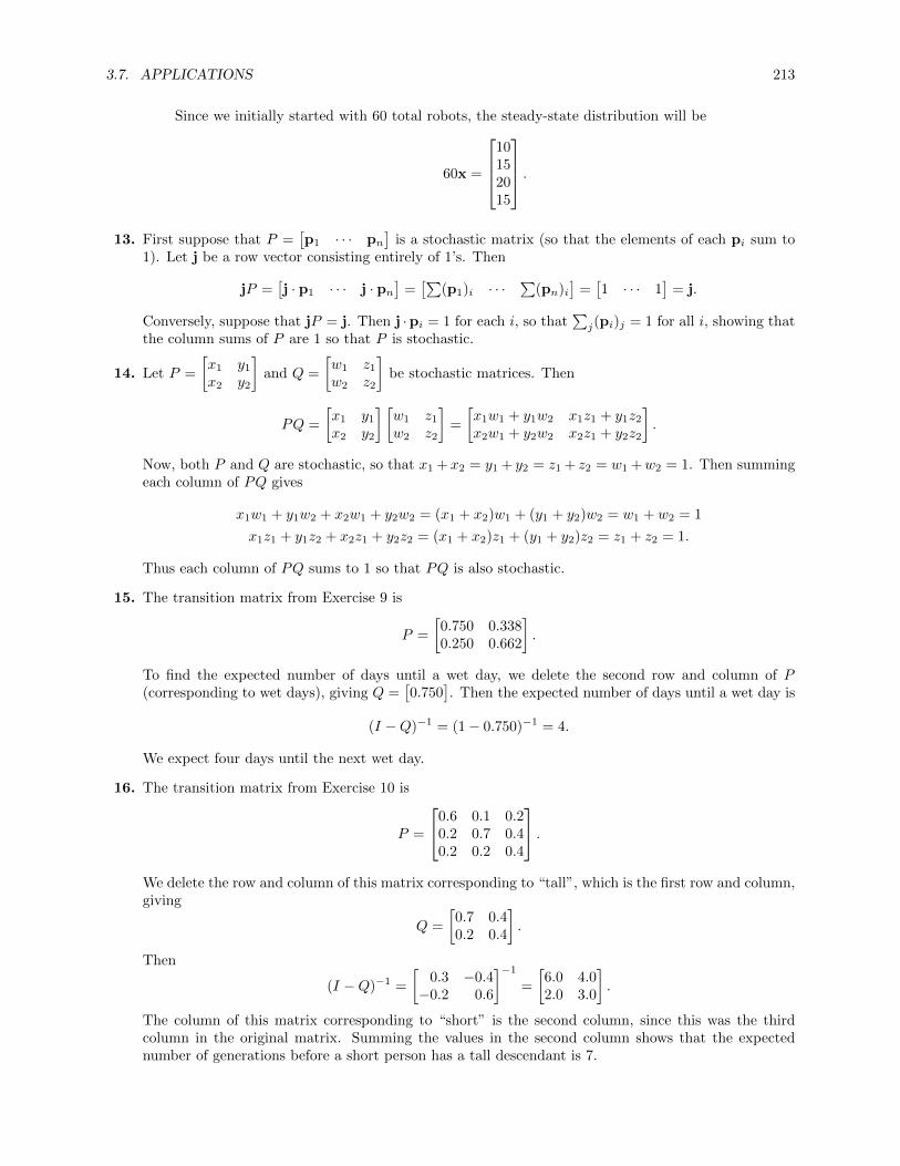
3.7. APPLICATIONS 213
Since we initially started with 60 total robots, the steady-state distribution will be
60x =
10152015
.13. First suppose that P =
[p1 · · · pn
]is a stochastic matrix (so that the elements of each pi sum to
1). Let j be a row vector consisting entirely of 1’s. Then
jP =[j · p1 · · · j · pn
]=[∑
(p1)i · · ·∑
(pn)i]
=[1 · · · 1
]= j.
Conversely, suppose that jP = j. Then j ·pi = 1 for each i, so that∑j(pi)j = 1 for all i, showing that
the column sums of P are 1 so that P is stochastic.
14. Let P =
[x1 y1
x2 y2
]and Q =
[w1 z1
w2 z2
]be stochastic matrices. Then
PQ =
[x1 y1
x2 y2
] [w1 z1
w2 z2
]=
[x1w1 + y1w2 x1z1 + y1z2
x2w1 + y2w2 x2z1 + y2z2
].
Now, both P and Q are stochastic, so that x1 +x2 = y1 + y2 = z1 + z2 = w1 +w2 = 1. Then summingeach column of PQ gives
x1w1 + y1w2 + x2w1 + y2w2 = (x1 + x2)w1 + (y1 + y2)w2 = w1 + w2 = 1
x1z1 + y1z2 + x2z1 + y2z2 = (x1 + x2)z1 + (y1 + y2)z2 = z1 + z2 = 1.
Thus each column of PQ sums to 1 so that PQ is also stochastic.
15. The transition matrix from Exercise 9 is
P =
[0.750 0.3380.250 0.662
].
To find the expected number of days until a wet day, we delete the second row and column of P(corresponding to wet days), giving Q =
[0.750
]. Then the expected number of days until a wet day is
(I −Q)−1 = (1− 0.750)−1 = 4.
We expect four days until the next wet day.
16. The transition matrix from Exercise 10 is
P =
0.6 0.1 0.20.2 0.7 0.40.2 0.2 0.4
.We delete the row and column of this matrix corresponding to “tall”, which is the first row and column,giving
Q =
[0.7 0.40.2 0.4
].
Then
(I −Q)−1 =
[0.3 −0.4−0.2 0.6
]−1
=
[6.0 4.02.0 3.0
].
The column of this matrix corresponding to “short” is the second column, since this was the thirdcolumn in the original matrix. Summing the values in the second column shows that the expectednumber of generations before a short person has a tall descendant is 7.
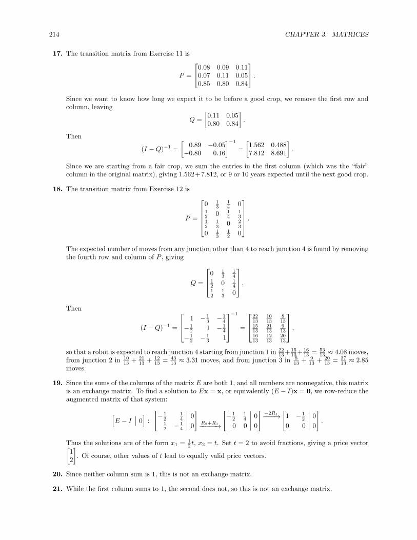
214 CHAPTER 3. MATRICES
17. The transition matrix from Exercise 11 is
P =
0.08 0.09 0.110.07 0.11 0.050.85 0.80 0.84
.Since we want to know how long we expect it to be before a good crop, we remove the first row andcolumn, leaving
Q =
[0.11 0.050.80 0.84
].
Then
(I −Q)−1 =
[0.89 −0.05−0.80 0.16
]−1
=
[1.562 0.4887.812 8.691
].
Since we are starting from a fair crop, we sum the entries in the first column (which was the “fair”column in the original matrix), giving 1.562+7.812, or 9 or 10 years expected until the next good crop.
18. The transition matrix from Exercise 12 is
P =
0 1
314 0
12 0 1
413
12
13 0 2
3
0 13
12 0
.The expected number of moves from any junction other than 4 to reach junction 4 is found by removingthe fourth row and column of P , giving
Q =
0 13
14
12 0 1
412
13 0
.Then
(I −Q)−1 =
1 − 13 − 1
4
− 12 1 − 1
4
− 12 − 1
3 1
−1
=
2213
1013
813
1513
2113
913
1613
1213
2013
,so that a robot is expected to reach junction 4 starting from junction 1 in 22
13 + 1513 + 16
13 = 5313 ≈ 4.08 moves,
from junction 2 in 1013 + 21
13 + 1213 = 43
13 ≈ 3.31 moves, and from junction 3 in 813 + 9
13 + 2013 = 37
13 ≈ 2.85moves.
19. Since the sums of the columns of the matrix E are both 1, and all numbers are nonnegative, this matrixis an exchange matrix. To find a solution to Ex = x, or equivalently (E − I)x = 0, we row-reduce theaugmented matrix of that system:
[E − I 0
]:
[− 1
214 0
12 − 1
4 0
]R2+R1−−−−−→
[− 1
214 0
0 0 0
]−2R1−−−→
[1 − 1
2 0
0 0 0
].
Thus the solutions are of the form x1 = 12 t, x2 = t. Set t = 2 to avoid fractions, giving a price vector[
12
]. Of course, other values of t lead to equally valid price vectors.
20. Since neither column sum is 1, this is not an exchange matrix.
21. While the first column sums to 1, the second does not, so this is not an exchange matrix.

3.7. APPLICATIONS 215
22. Since the sums of the columns of the matrix E are both 1, and all numbers are nonnegative, this matrixis an exchange matrix. To find a solution to Ex = x, or equivalently (E − I)x = 0, we row-reduce theaugmented matrix of that system:
[E − I 0
]:
[−0.9 0.6 0
0.9 −0.6 0
]R2+R1−−−−−→
[−0.9 0.6 0
0 0 0
] − 109 R1−−−−→
[1 − 2
3 00 0 0
].
Thus the solutions are of the form x1 = 23 t, x2 = t. Set t = 3 to avoid fractions, giving a price vector[
23
]. Of course, other values of t lead to equally valid price vectors.
23. Since the matrix contains a negative entry, it is not an exchange matrix.
24. Since the sums of the columns of the matrix E are both 1, and all numbers are nonnegative, this matrixis an exchange matrix. To find a solution to Ex = x, or equivalently (E − I)x = 0, we row-reduce theaugmented matrix of that system:
[E − I 0
]:
−12 1 0 0
0 −1 13 0
12 0 − 1
3 0
−R2−−−→R3+R1−−−−−→
−12 1 0 0
0 1 − 13 0
0 1 − 13 0
R1−R2−−−−−→
R3−R2−−−−−→−12 0 1
3 0
0 1 − 13 0
0 0 0 0
−2R1−−−→
1 0 − 23 0
0 1 − 13 0
0 0 0 0
.Thus the solutions are of the form x1 = 2
3 t, x2 = 13 t, x3 = t. Set t = 3 to avoid fractions, giving a price
vector
213
. Of course, other values of t lead to equally valid price vectors.
25. Since the sums of the columns of the matrix E are both 1, and all numbers are nonnegative, this matrixis an exchange matrix. To find a solution to Ex = x, or equivalently (E − I)x = 0, we row-reduce theaugmented matrix of that system:
[E − I 0
]:
−0.7 0 0.2 0
0.3 −0.5 0.3 0
0.4 0.5 −0.5 0
− 10
7 R1−−−−→ 1 0 − 2
7 0
0.3 −0.5 0.3 0
0.4 0.5 −0.5 0
R2−0.3R1−−−−−−→R3−0.4R1−−−−−−→
1 0 − 27 0
0 − 12
2770 0
0 12 − 27
70 0
R3+R2−−−−−→
1 0 − 27 0
0 − 12
2770 0
0 0 0 0
−2R2−−−→
1 0 − 27 0
0 1 − 2735 0
0 0 0 0
.Thus the solutions are of the form x1 = 2
7 t, x2 = 2735 t, x3 = t. Set t = 35 to avoid fractions, giving a
price vector
102735
. Of course, other values of t lead to equally valid price vectors.
26. Since the sums of the columns of the matrix E are both 1, and all numbers are nonnegative, this matrixis an exchange matrix. To find a solution to Ex = x, or equivalently (E − I)x = 0, we row-reduce the

216 CHAPTER 3. MATRICES
augmented matrix of that system:
[E − I 0
]:
−0.50 0.70 0.35 0
0.25 −0.70 0.25 0
0.25 0 −0.6 0
−2R1−−−→
1 −1.40 −0.70 0
0.25 −0.70 0.25 0
0.25 0 −0.6 0
R2−0.25R1−−−−−−−→R3−0.25R1−−−−−−−→1 −1.40 −0.70 0
0 −0.35 0.425 00 0.35 −0.425 0
R1−4R2−−−−−→
R3+R2−−−−−→
1 0 −2.40 00 −0.35 0.425 00 0 0 0
− 13.5R2−−−−−→
1 0 −2.40 00 1 −1.214 00 0 0 0
So one possible solution is
2.41.214
1
. Multiplying through by 70 will roughly clear fractions, giving
≈
1688570
if an integral solution is desired.
27. This matrix is a consumption matrix since all of its entries are nonnegative. By Corollary 3.36, it isproductive since the sum of the entries in each column is strictly less than 1. (Note that Corollary 3.35does not apply since the sum of the entries in the second row exceeds 1).
28. This matrix is a consumption matrix since all of its entries are nonnegative. By Corollary 3.35, it isproductive since the sum of the entries in each row is strictly less than 1. (Note that Corollary 3.36does not apply since the sum of the entries in the third column exceeds 1).
29. This matrix is a consumption matrix since all of its entries are nonnegative. Since the entries in thesecond row as well as those in the second column sum to a number greater than 1, neither Corollary3.35 nor 3.36 applies. So to determine if C is productive, we must use the definition, which involvesseeing if I − C is invertible and if its inverse has all positive entries.
I − C =
1 0 00 1 00 0 1
−0.35 0.25 0
0.15 0.55 0.350.45 0.30 0.60
=
0.65 −0.25 0−0.15 0.45 −0.35−0.45 −0.30 0.40
.Using technology,
(I − C)−1 ≈
−13.33 −17.78 −15.56−38.67 −46.22 −40.44−44.00 −54.67 −45.33
.Since this is not a positive matrix, it follows that C is not productive.
30. This matrix is a consumption matrix since all of its entries are nonnegative. Since the entries in thefirst row as well as those in the each column sum to a number at least equal to 1, neither Corollary3.35 nor 3.36 applies. So to determine if C is productive, we must use the definition, which involvesseeing if I − C is invertible and if its inverse has all positive entries.
I − C =
1 0 0 00 1 0 00 0 1 00 0 0 1
−
0.2 0.4 0.1 0.40.3 0.2 0.2 0.10 0.4 0.5 0.3
0.5 0 0.2 0.2
=
0.8 −0.4 −0.1 −0.4−0.3 0.8 −0.2 −0.1
0 −0.4 0.5 −0.3−0.5 0 −0.2 0.8
.Using technology reveals that I − C is not invertible, so that C is not productive.
31. To find a solution x to (I − C)x = d, we invert I − C and compute x = (I − C)−1d. Here
I − C =
[1 0
0 1
]−
[12
14
12
12
]=
[12 − 1
4
− 12
12
].

3.7. APPLICATIONS 217
Then det(I − C) = 12 ·
12 −
(− 1
4
) (− 1
2
)= 1
8 , so that
(I − C)−1 =1
1/8
[12
14
12
12
]=
[4 2
4 4
].
Thus a feasible production vector is
x = (I − C)−1d =
[4 24 4
] [13
]=
[1016
].
32. To find a solution x to (I − C)x = d, we invert I − C and compute x = (I − C)−1d. Here
I − C =
[1 00 1
]−[0.1 0.40.3 0.2
]=
[0.9 −0.4−0.3 0.8
].
Then det(I − C) = 0.9 · 0.8− (−0.4)(−0.3) = 0.60, so that
(I − C)−1 =1
0.60
[0.8 0.4
0.3 0.9
]=
[43
23
12
32
].
Thus a feasible production vector is
x = (I − C)−1d =
[43
23
12
32
][2
1
]=
[10352
].
33. To find a solution x to (I − C)x = d, we invert I − C and compute x = (I − C)−1d. Here
I − C =
1 0 00 1 00 0 1
−0.5 0.2 0.1
0 0.4 0.20 0 0.5
=
0.5 −0.2 −0.10 0.6 −0.80 0 0.5
.Then row-reduce
[I − C I
]to compute (I − C)−1:
[I − C I
]=
0.5 −0.2 −0.1 1 0 0
0 0.6 −0.8 0 1 0
0 0 0.5 0 0 1
→1 0 0 2 2
323
0 1 0 0 53
23
0 0 1 0 0 2
.Thus a feasible production vector is
x = (I − C)−1d =
2 23
23
0 53
23
0 0 2
3
2
4
=
10
6
8
.34. To find a solution x to (I − C)x = d, we invert I − C and compute x = (I − C)−1d. Here
I − C =
1 0 00 1 00 0 1
−0.1 0.4 0.1
0 0.2 0.20.3 0.2 0.3
=
0.9 −0.4 −0.10 0.8 −0.2
−0.3 −0.2 0.7
.Compute (I − C)−1 using technology to get
(I − C)−1 ≈
1.238 0.714 0.3810.143 1.429 0.4290.571 0.714 1.714
.Thus a feasible production vector is
x = (I − C)−1d =
1.238 0.714 0.381
0.143 1.429 0.429
0.571 0.714 1.714
1.1
3.5
2.0
=
4.624
6.014
6.557
.

218 CHAPTER 3. MATRICES
35. Since x ≥ 0 and A ≥ O, then Ax has all nonnegative entries as well, so that Ax ≥ Ox = 0. But then
x > Ax ≥ Ox = 0,
so that x > 0.
36. (a) Since all entries of all matrices are positive, it is clear that AC ≥ O and BD ≥ O. To see thatAC ≥ BD, let A = (aij), B = (bij), C = (cij), and D = (dij). Then each aij ≥ bij and eachcij ≥ dij . So
(AC)ij =
n∑k=1
aikckj ≥n∑k=1
bikckj ≥n∑k=1
bikdkj = (BD)ij .
So every entry of AC is greater than or equal to the corresponding entry of BD, and thusAC ≥ BD.
(b) Let xT =[x1 x2 · · · xn
]. Then for any i and j, we know that aijxj ≥ bijxj since aij > bij
and xj ≥ 0. Since x 6= 0, we know that some component of x, say xk, is strictly positive. Thenaikxk > bikxk since xk > 0. But then
(Ax)i = ai1x1 + · · ·+ aikxk + · · ·+ ainxn > bi1x1 + · · ·+ bikxk + · · ·+ binxn = (Bx)i.
37. Multiplying, we get
x1 = Lx0 =
[2 5
0.6 0
] [105
]=
[456
]x2 = Lx1 =
[2 5
0.6 0
] [456
]=
[12022.5
]x3 = Lx2 =
[2 5
0.6 0
] [12027
]=
[37572
]38. Multiplying, we get
x1 = Lx0 =
0 1 20.2 0 00 0.5 0
1043
=
1022
x2 = Lx1 =
0 1 20.2 0 00 0.5 0
1022
=
621
x3 = Lx2 =
0 1 20.2 0 00 0.5 0
621
=
41.21
39. Multiplying, we get
x1 = Lx0 =
1 1 30.7 0 00 0.5 0
100100100
=
5007050
x2 = Lx1 =
1 1 30.7 0 00 0.5 0
5007050
=
72035035
x3 = Lx2 =
1 1 30.7 0 00 0.5 0
72035035
=
1175504175
.

3.7. APPLICATIONS 219
40. Multiplying, we get
x1 = Lx0 =
0 1 2 5
0.5 0 0 00 0.7 0 00 0 0.3 0
10101010
=
80573
x2 = Lx1 =
0 1 2 5
0.5 0 0 00 0.7 0 00 0 0.3 0
80573
=
34403.52.1
x3 = Lx2 =
0 1 2 5
0.5 0 0 00 0.7 0 00 0 0.3 0
34403.52.1
=
57.51728
1.05
.
41. (a) The first ten generations of the species using each of the two models are as follows:
x0 x1 x2 x3 x4 x5
L1
[1010
] [508
] [4040
] [20032
] [160160
] [800128
]
L2
[1010
] [508
] [20840
] [872
166.4
] [3654.4697.6
] [15315.22923.52
]x6 x7 x8 x9 x10
L1
[640640
] [3200512
] [25602560
] [128002048
] [1024010240
]
L2
[64184.312252.2
] [26898951347.5
] [1.127× 10⁶
215192
] [4.724× 10⁶
901844
] [1.980× 10⁷
3.780× 10⁶
].
(b) Graphs of the first ten generations using each model are:
Class 1
Class 20 2 4 6 8 10
TimeHyrsL
0.2
0.4
0.6
0.8
1.0
PercentageModel L1
Class 1
Class 2
0 2 4 6 8 10TimeHyrsL
0.2
0.4
0.6
0.8
1.0
PercentageModel L2
The graphs suggest that the first model does not have a steady state, while the second Lesliematrix quickly approaches a steady state ratio of class 1 to class 2 population.

220 CHAPTER 3. MATRICES
42. Start with x0 =
202020
. Then
x1 =
0 0 200.1 0 00 0.5 0
202020
=
400210
x2 =
0 0 200.1 0 00 0.5 0
400210
=
200401
x3 =
0 0 200.1 0 00 0.5 0
200401
=
202020
.Thus after three generations the population is back to where it started, so that the population is cyclic.
43. Start with x0 =
202020
. Then
x1 =
0 0 20s 0 00 0.5 0
202020
=
40020s10
x2 =
0 0 20s 0 00 0.5 0
40020s10
=
200400s10s
x3 =
0 0 20s 0 00 0.5 0
200400s10s
=
200s200s200s
.Thus after three generations the population is still evenly distributed among the three classes, but thetotal population has been multiplied by 10s. So
• If s < 0.1, then the overall population declines after three years;
• If s = 0.1, then the overall population is cyclic every three years;
• If s > 0.1, then the overall population increases after three years.
44. The table gives us seven separate age classes, each of duration two years; from the table, the Lesliematrix of the system is
L =
0 0.4 1.8 1.8 1.8 1.6 0.60.3 0 0 0 0 0 00 0.7 0 0 0 0 00 0 0.9 0 0 0 00 0 0 0.9 0 0 00 0 0 0 0.9 0 00 0 0 0 0 0.6 0
.
Since in 1990,
x0 =
102851201
, so that x1 = Lx0 =
46.43
1.47.24.510.8
0
, and x2 = Lx1 =
42.0613.922.11.266.484.056.48
.

3.7. APPLICATIONS 221
Then x1 and x2 represent the population distribution in 1991 and 1992. To project the population forthe years 2000 and 2010, note that xn = Lnx0. Thus
x10 = L10x0 ≈
69.1218.6112.2410.598.296.513.57
, x20 = L20x0 ≈
167.8046.0829.5424.3520.0616.489.05
.
45. The adjacency matrix contains a 1 in row i, column j if there is an edge between vi and vj :0 1 0 11 0 1 00 1 0 11 0 1 0
.46. The adjacency matrix contains a 1 in row i, column j if there is an edge between vi and vj :
1 0 0 10 1 1 00 1 0 01 0 0 0
.47. The adjacency matrix contains a 1 in row i, column j if there is an edge between vi and vj :
0 1 1 1 11 0 1 0 01 1 0 1 01 0 1 0 11 0 0 1 0
.
48. The adjacency matrix contains a 1 in row i, column j if there is an edge between vi and vj :0 0 0 1 10 0 0 1 00 0 0 1 01 1 1 0 01 0 0 0 0
.
49.
v1
v2
v3
v4

222 CHAPTER 3. MATRICES
50.
v1
v2
v3
v4
51.
v1v2
v3
v4
v5
52.
v1
v2
v3
v4
v5
53. The adjacency matrix contains a 1 in row i, column j if there is an edge from vi to vj :0 1 1 00 0 0 00 1 0 11 0 0 0
.54. The adjacency matrix contains a 1 in row i, column j if there is an edge from vi to vj :
0 0 1 10 0 0 11 1 0 00 1 1 0
.

3.7. APPLICATIONS 223
55. The adjacency matrix contains a 1 in row i, column j if there is an edge from vi to vj :0 1 0 1 01 0 0 1 01 1 0 0 01 0 0 0 11 0 0 0 0
.
56. The adjacency matrix contains a 1 in row i, column j if there is an edge from vi to vj :0 1 0 1 10 0 0 0 10 1 0 1 00 0 0 0 10 0 1 0 0
.
57.
v1
v2
v3
v4
58.
v1 v2
v3 v4
59.v1
v2v3
v4
v5

224 CHAPTER 3. MATRICES
60.
v1
v2
v3v4
v5
61. In Exercise 50,
A =
0 1 0 11 1 1 10 1 0 11 1 1 0
, so A2 =
2 2 2 12 4 2 32 2 2 11 3 1 3
.The number of paths of length 2 between v1 and v2 is given by
(A2)
12= 2. So there are two paths of
length 2 between v1 and v2.
62. In Exercise 52,
A =
0 0 0 1 10 0 0 1 10 0 0 1 11 1 1 0 01 1 1 0 0
, so A2 =
2 2 2 0 02 2 2 0 02 2 2 0 00 0 0 3 30 0 0 3 3
.The number of paths of length 2 between v1 and v2 is given by
(A2)
12= 2. So there are two paths of
length 2 between v1 and v2.
63. In Exercise 50,
A =
0 1 0 11 1 1 10 1 0 11 1 1 0
, so A3 =
3 7 3 67 11 7 83 7 3 66 8 6 5
.The number of paths of length 3 between v1 and v3 is given by
(A3)
13= 3. So there are three paths
of length 3 between v1 and v3.
64. In Exercise 52,
A =
0 0 0 1 10 0 0 1 10 0 0 1 11 1 1 0 01 1 1 0 0
, so A4 =
12 12 12 0 012 12 12 0 012 12 12 0 00 0 0 18 180 0 0 18 18
.The number of paths of length 4 between v2 and v2 is given by
(A4)
22= 12. So there are twelve paths
of length 4 between v2 and itself.

3.7. APPLICATIONS 225
65. In Exercise 57,
A =
0 1 0 01 0 0 10 1 0 01 0 1 1
, so A2 =
1 0 0 11 1 1 11 0 0 11 2 1 1
.The number of paths of length 2 from v1 to v3 is
(A2)
13= 0. There are no paths of length 2 from v1
to v3.
66. In Exercise 57,
A =
0 1 0 01 0 0 10 1 0 01 0 1 1
, so A3 =
1 1 1 12 2 1 21 1 1 13 2 1 3
.The number of paths of length 3 from v4 to v1 is
(A3)
41= 3. There are three paths of length 3 from
v4 to v1.
67. In Exercise 60,
A =
0 1 0 0 10 0 0 1 01 0 0 1 11 0 1 0 01 1 0 0 0
, so A3 =
1 1 1 1 11 1 0 1 22 3 0 3 33 3 1 1 12 1 1 1 0
.The number of paths of length 3 from v4 to v1 is
(A3)
41= 3. There are three paths of length 3 from
v4 to v1.
68. In Exercise 60,
A =
0 1 0 0 10 0 0 1 01 0 0 1 11 0 1 0 01 1 0 0 0
, so A4 =
3 2 1 2 23 3 1 1 16 5 3 3 23 4 1 4 42 2 1 2 3
.The number of paths of length 4 from v1 to v4 is
(A3)
14= 2. There are two paths of length 4 from v1
to v4.
69. (a) If there are no ones in row i, then no edges join vertex i to any of the other vertices. Thus G is adisconnected graph, and vertex i is an isolated vertex.
(b) If there are no ones in column j, then no edges join vertex j to any of the other vertices. Thus Gis a disconnected graph, and vertex j is an isolated vertex.
70. (a) If row i of A2 is all zeros, then there are no paths of length 2 from vertex i to any other vertex.
(b) If column j of A2 is all zeros, then there are no paths of length 2 from any vertex to vertex j.
71. The adjacency matrix for the digraph is
A =
0 0 0 0 1 01 0 1 0 1 11 0 0 1 1 01 1 0 0 1 00 0 0 0 0 11 0 1 1 0 0
.
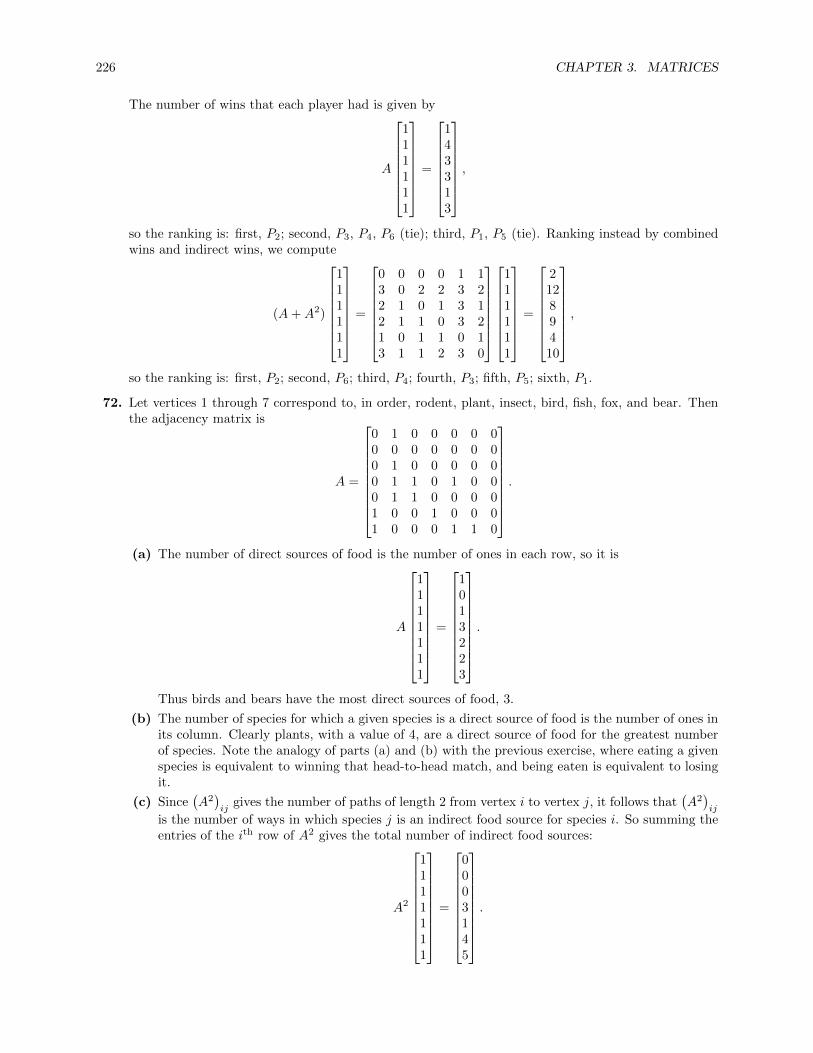
226 CHAPTER 3. MATRICES
The number of wins that each player had is given by
A
111111
=
143313
,
so the ranking is: first, P2; second, P3, P4, P6 (tie); third, P1, P5 (tie). Ranking instead by combinedwins and indirect wins, we compute
(A+A2)
111111
=
0 0 0 0 1 13 0 2 2 3 22 1 0 1 3 12 1 1 0 3 21 0 1 1 0 13 1 1 2 3 0
111111
=
21289410
,
so the ranking is: first, P2; second, P6; third, P4; fourth, P3; fifth, P5; sixth, P1.
72. Let vertices 1 through 7 correspond to, in order, rodent, plant, insect, bird, fish, fox, and bear. Thenthe adjacency matrix is
A =
0 1 0 0 0 0 00 0 0 0 0 0 00 1 0 0 0 0 00 1 1 0 1 0 00 1 1 0 0 0 01 0 0 1 0 0 01 0 0 0 1 1 0
.
(a) The number of direct sources of food is the number of ones in each row, so it is
A
1111111
=
1013223
.
Thus birds and bears have the most direct sources of food, 3.
(b) The number of species for which a given species is a direct source of food is the number of ones inits column. Clearly plants, with a value of 4, are a direct source of food for the greatest numberof species. Note the analogy of parts (a) and (b) with the previous exercise, where eating a givenspecies is equivalent to winning that head-to-head match, and being eaten is equivalent to losingit.
(c) Since(A2)ij
gives the number of paths of length 2 from vertex i to vertex j, it follows that(A2)ij
is the number of ways in which species j is an indirect food source for species i. So summing theentries of the ith row of A2 gives the total number of indirect food sources:
A2
1111111
=
0003145
.
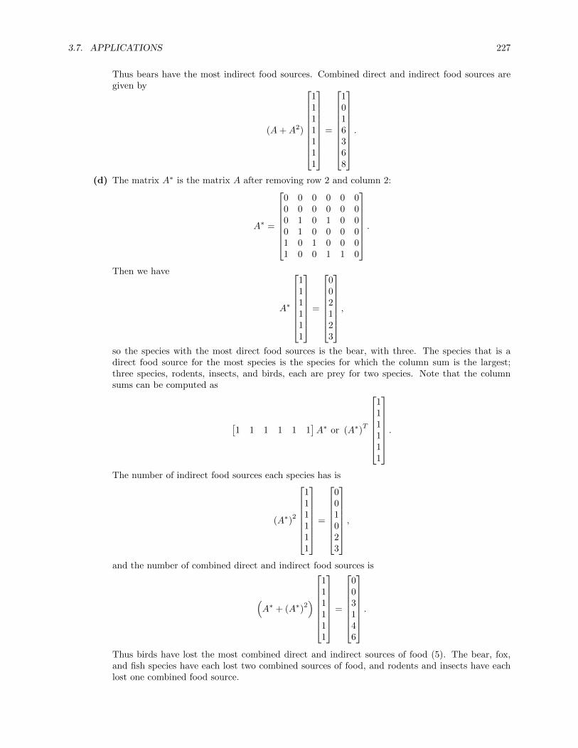
3.7. APPLICATIONS 227
Thus bears have the most indirect food sources. Combined direct and indirect food sources aregiven by
(A+A2)
1111111
=
1016368
.
(d) The matrix A∗ is the matrix A after removing row 2 and column 2:
A∗ =
0 0 0 0 0 00 0 0 0 0 00 1 0 1 0 00 1 0 0 0 01 0 1 0 0 01 0 0 1 1 0
.
Then we have
A∗
111111
=
002123
,so the species with the most direct food sources is the bear, with three. The species that is adirect food source for the most species is the species for which the column sum is the largest;three species, rodents, insects, and birds, each are prey for two species. Note that the columnsums can be computed as
[1 1 1 1 1 1
]A∗ or (A∗)
T
111111
.
The number of indirect food sources each species has is
(A∗)2
111111
=
001023
,
and the number of combined direct and indirect food sources is
(A∗ + (A∗)
2)
111111
=
003146
.
Thus birds have lost the most combined direct and indirect sources of food (5). The bear, fox,and fish species have each lost two combined sources of food, and rodents and insects have eachlost one combined food source.

228 CHAPTER 3. MATRICES
(e) Since (A∗)5
is the zero matrix, after a while, no species will have a direct food source, so that theecosystem will be wiped out.
73. (a) Using the relationships given, we get the digraph
Ann
Bert
Carla
Dana
Ehaz
Letting vertices 1 through 5 correspond to the people in alphabetical order, the adjacency matrixis
A =
0 0 1 0 10 0 1 1 00 0 0 0 11 0 1 0 00 1 0 0 0
.(b) The element
[Ak]ij
is 1 if there is a path of length k from i to j, so there is a path of length at
most k from i to j if[A+A2 + · · ·+Ak
]ij≥ 1. If Bert hears a rumor and we want to know how
many steps it takes before everyone else has heard the rumor, then we must calculate A, A+A2,A + A2 + A3, and so forth, until every entry in row 2 (except for the one in column 2, whichcorresponds to Bert himself) is nonzero. This is not true for A, since for example A21 = 0. Next,
A+A2 =
0 1 1 0 21 0 2 1 10 1 0 0 11 0 2 0 20 1 1 1 0
,so everyone else will have heard the rumor, either directly or indirectly, from Bert after two steps(Carla will have heard it twice).
(c) Using the same logic as in part (b), we must compute successive sums of powers of A until everyentry in the first row, except for the entry in the first column corresponding to Ann herself, isnonzero. From part (b), we see that this is not the case for A+A2 since
[A+A2
]14
= 0. Next,
A+A2 +A3 =
0 2 2 1 21 1 3 1 30 1 1 1 11 2 2 0 31 1 2 1 1
,so everyone else will have heard the rumor from Ann after three steps. In fact, everyone but Danawill have heard it twice.
(d) j is reachable from i by a path of length k if[Ak]ij
is nonzero. Now, if j is reachable from i at
all, it is reachable by a path of length at most n, where n is the number of vertices in the digraph,so we must compute [
A+A2 +A3 + · · ·+An]ij
and see if it is nonzero. If it is, the two vertices are connected.

3.7. APPLICATIONS 229
74. Let G be a graph with m vertices, and A = (aij) its adjacency matrix.
(a) The basis for the induction is n = 1, where the statement says that aij is the number of directpaths between vertices i and j. But this is just the definition of the adjacency matrix, sinceaij = 1 if i and j have an edge between them and is zero otherwise. Next, assume [Ak]ij is thenumber of paths of length k between i and j. Then [Ak+1]ij =
∑ml=1[Ak]il[A]lj . For a given vertex
l, [Ak]il gives the number of paths of length k from i to l, and [A]lj gives the number of pathsof length 1 from l to j (this is either zero or one). So the product gives the number of paths oflength k+1 from i to j passing through l. Summing over all vertices l in the graph gives all pathsof length k + 1 from i to j, proving the inductive step.
(b) If G is a digraph, the statement of the result must be modified to say that the (i, j) entry of An
is equal to the number of n-paths from i to j; the proof is valid since the adjacency matrix of adigraph takes arrow directions into account.
75. [AAT ]ij =∑mk=1 aikajk. So this matrix entry is the number of vertices k that have edges from both
vertex i and vertex j.
76. From the diagram in Exercise 49, this graph is bipartite, with U = {v1} and V = {v2, v3, v4}.
77. From the diagram in Exercise 52, this graph is bipartite, with U = {v1, v2, v3} and V = {v4, v5}.
78. The graph in Exercise 51 is not bipartite. For suppose v1 ∈ U . Then since there are edges from v1 toboth v3 and v4, we must have v3, v4 ∈ V . Next, there are edges from v3 to v5, and from v4 to v2, sothat v2, v5 ∈ U . But there is an edge from v2 to v5. So this graph cannot be bipartite.
79. Examining the matrix, we see that vertices 1, 2, and 4 are connected to vertices 3, 5, and 6 only, sothat if we define U = {v1, v2, v4} and V = {v3, v5, v6}, we have shown that this graph is bipartite.
80. Suppose that G has n vertices.
(a) First suppose that the adjacency matrix of G is of the form shown. Suppose that the zero blockshave p and q = n− p rows respectively. Then any edges at vertices v1, v2, . . . , vp have their othervertex in vertices vp+1, vp+2, . . . , vn, since the upper left p × p matrix is O. Similarly, any edgesat vertices vp+1, vp+2, . . . , vn have their other vertex in vertices v1, v2, . . . , vp, since the lower rightq × q matrix is O. So G is bipartite, with U = {v1, v2, . . . , vp} and V = {vp+1, vp+2, . . . , vn}.Next suppose that G is bipartite. Label the vertices so that U = {v1, v2, . . . , vp} and V ={vp+1, vp+2, . . . , vn}. Now consider the adjacency matrix A of G. aij = 0 if i, j ≤ p, since thenboth vi and vj are in U ; similarly, aij = 0 if i, j > p, since then both vi and vj are in V . So theupper left p× p submatrix as well as the bottom right q × q submatrix are the zero matrix. Theremaining two submatrices are transposes of each other since this is an undirected graph, so thataij = 1 if and only if aji = 1. Thus A is of the form shown.
(b) Suppose G is bipartite and A its adjacency matrix, of the form given in part (a). It suffices toshow that odd powers of A have zero blocks at upper left of size p× p and at lower right of sizeq × q, since then there are no paths of odd length between any vertex and itself. We do this byinduction. Clearly A1 = A is of that form. Now,
A2 =
[OO +BBT OB +BOBTO +OBT BTB +OO
]=
[BBT OO BTB
]=
[D1 OO D2
]where D1 = BBT and D2 = BTB. Suppose that A2k−1 has the required zero blocks. Then
A2k+1 = A2k−1A2 =
[O C1
C2 O
] [D1 OO D2
]=
[OD1 + C1O OO + C1D2
C2D1 +OO D1O +OD2
]=
[O C1D2
C2D1 O
].

230 CHAPTER 3. MATRICES
Thus A2k+1 is of this form as well. So no odd power of A has any entries in the upper left orlower right block, so there are no odd paths beginning and ending at the same vertex. Thus allcircuits must be of even length. (Note that in the matrix A2k+1 above, we must in fact have(C1D2)T = C2D1 since powers of a symmetric matrix are symmetric, but we do not need thisfact.)
Chapter Review
1. (a) True. See Exercise 34 in Section 3.2. If A is an m×n matrix, then AT is an n×m matrix. ThenAAT is defined and is an m×m matrix, and ATA is also defined and is an n× n matrix.
(b) False. This is true only when A is invertible. For example, if
A =
[1 00 1
], B =
[0 00 1
], then AB =
[0 00 0
],
but A 6= O.
(c) False. What is true is that XAA−1 = BA−1 so that X = BA−1. Matrix multiplication is notcommutative, so that BA−1 6= A−1B in general.
(d) True. This is Theorem 3.11 in Section 3.3.
(e) True. If E performs kRi, then E is a matrix with all zero entries off the diagonal, so it is itsown transpose and thus ET is also the elementary matrix that performs kRi. If E performsRi + kRj , then the only off-diagonal entry in E is [E]ij = k, so the only off-diagonal entry of ET
is [ET ]ji = k and thus ET is the elementary matrix performing Rj + kRi. Finally, if E performsRi ↔ Rj , then [E]ii = [E]jj = 0 and [E]ij = [E]ji = 1, so that ET = E and thus ET is also anelementary matrix exchanging Ri and Rj .
(f) False. Elementary matrices perform a single row operation, while their products can perform mul-tiple row operations. There are many examples. For instance, consider the elementary matricescorresponding to R1 ↔ R2 and 2R1:[
0 11 0
] [2 00 1
]=
[0 12 0
],
which is not an elementary matrix.
(g) True. See Theorem 3.21 in Section 3.5.
(h) False. For this to be true, the plane must pass through the origin.
(i) True, since
T (c1u + c2v) = −(c1u + c2v) = −c1u− c2v = c1(−u) + c2(−v) = c1T (u) + c2T (v).
(j) False; the matrix is 5× 4, not 4× 5. See Theorems 3.30 and 3.31 in Section 3.6.
2. Since A is 2× 2, so is A2. Since B is 2× 3, the product makes sense. Then
A2 =
[1 23 5
] [1 23 5
]=
[7 1218 31
], so that A2B =
[7 1218 31
] [2 0 −13 −3 4
]=
[50 −36 41
129 −93 106
].
3. B2 is not defined, since the number of columns of B is not equal to the number of rows of B. So thismatrix product does not make sense.
4. Since BT is 3 × 2, A−1 is 2 × 2, and B is 2 × 3, this matrix product makes sense as long as A isinvertible. Since detA = 1 · 5− 2 · 3 = −1, we have
A−1 =1
−1
[5 −2−3 1
]=
[−5 2
3 −1
],

Chapter Review 231
so that
BTA−1B =
2 30 −3−1 4
[−5 23 −1
] [2 0 −13 −3 4
]=
−1 1−9 317 −6
[2 0 −13 −3 4
]=
1 −3 5−9 −9 2116 18 −41
.5. Since BBT is always defined (see exercise 34 in section 3.2) and is square, (BBT )−1 makes sense if
BBT is invertible. We have
BBT =
[2 0 −13 −3 4
] 2 30 −3−1 4
=
[5 22 34
].
Then det(BBT ) = 5 · 34− 22̇ = 166, so that
(BBT )−1 =1
166
[34 −2−2 5
].
6. Since BTB is always defined (see exercise 34 in section 3.2) and is square, (BTB)−1 makes sense ifBTB is invertible. We have
BTB =
2 30 −3−1 4
[2 0 −13 −3 4
]=
13 −9 10−9 9 −1210 −12 17
.To compute the inverse, we row-reduce
[BTB I
]:
[BTB I
]=
13 −9 10 1 0 0
−9 9 −12 0 1 0
10 −12 17 0 0 1
R2+ 913R1−−−−−−→
R3− 1013R1−−−−−−→
13 −9 10 1 0 0
0 3613 − 66
13913 1 0
0 − 6613
12113 − 10
13 0 1
R3+ 6636R2−−−−−−→
13 −9 10 1 0 0
0 3613 − 66
13913 1 0
0 0 0 12
116 1
.Since the matrix on the left has a zero row, BTB is not invertible, so (BTB)−1 does not exist.
7. The outer product expansion of AAT is
AAT = a1AT1 + a2A
T2 =
[13
] [1 3
]+
[25
] [2 5
]=
[1 33 9
]+
[4 1010 25
]=
[5 1313 34
].
8. By Theorem 3.9 in Section 3.3, we know that (A−1)−1 = A, so we must find the inverse of the givenmatrix. Now, detA−1 = 1
2 · 4− (−1)(− 3
2
)= 1
2 , so that
A = (A−1)−1 =1
1/2
[4 132
12
]=
[8 2
3 1
].
9. Since AX = B =
−1 −35 03 −2
, we have X = A−1B. To find A−1, we compute
1 0 −1 1 0 0
2 3 −1 0 1 0
0 1 1 0 0 1
→1 0 0 2 − 1
232
0 1 0 −1 12 − 1
2
0 0 1 1 − 12
32
.

232 CHAPTER 3. MATRICES
Then
X = A−1B =
2 − 12
32
−1 12 − 1
2
1 − 12
32
−1 −3
5 0
3 −2
=
0 −9
2 4
1 −6
.10. Since detA = 1 ·6−2 ·4 = −2 6= 0, A is invertible, so by Theorem 3.12 in Section 3.3, it can be written
as a product of elementary matrices. As in Example 3.29 in Section 3.3, we start by row-reducing A:
A =
[1 24 6
]R2−4R1−−−−−→
[1 20 −2
]− 1
2R2−−−−→
[1 20 1
]R1−2R2−−−−−→
[1 00 1
].
So by applying
E1 =
[1 0
4 1
], E2 =
[1 0
0 − 12
], E3 =
[1 −2 0 1
]in that order to A we get the identity matrix, so that E3E2E1A = I. Since elementary matrices areinvertible, this means that A = (E3E2E1)−1 = E−1
1 E−12 E−1
3 . Since E1 is R2 − 4R1, it follows thatE−1
1 is R2 + 4R1. Since E2 is − 12R2, it follows that E−1
2 is −2R2. Since E3 is R1− 2R2, it follows that
E−13 is R1 + 2R2. Thus
A = E−11 E−1
2 E−13 =
[1 0−1 1
] [1 00 −2
] [1 20 1
].
11. To show that (I −A)−1 = I +A+A2, it suffices to show that (I +A+A2)(I −A) = I. But
(I+A+A2)(I−A) = II−IA+AI−A2 +A2I−A3 = I−A+A−A2 +A2−A3 = I+A3 = I+O = I.
12. Use the multiplier method. We want to reduce A to an upper triangular matrix:
A =
1 1 13 1 12 −1 1
R2−3R1−−−−−→R3−2R1−−−−−→
1 1 10 −2 −20 −3 −1
R3− 3
2R2−−−−−−→
1 1 10 −2 −20 0 2
= U.
Then `21 = 3, `31 = 2, and `32 = 32 , so that
L =
1 0 0
3 1 0
2 32 1
.13. We follow the comment after Example 3.48 in Section 3.5. Start by finding the reduced row echelon
form of A:2 −4 5 8 51 −2 2 3 14 −8 3 2 6
R1↔R2−−−−−→
1 −2 2 3 12 −4 5 8 54 −8 3 2 6
R2−2R1−−−−−→R3−4R1−−−−−→
1 −2 2 3 10 0 1 2 30 0 −5 −10 2
R3+5R2−−−−−→
1 −2 2 3 10 0 1 2 30 0 0 0 8
18R3−−−→
1 −2 2 3 10 0 1 2 30 0 0 0 1
R1−R3−−−−−→R2−3R3−−−−−→
1 −2 2 3 00 0 1 2 00 0 0 0 1
R1−2R2−−−−−→1 −2 0 −1 0
0 0 1 2 00 0 0 0 1
.

Chapter Review 233
Thus a basis for row(A) is given by the nonzero rows of the matrix, or
{[1 −2 0 −1 0
],[0 0 1 2 0
],[0 0 0 0 1
]}.
Note that since the matrix is rank 3, so all three rows are nonzero, the rows of the original matrix alsoprovide a basis for row(A).
A basis for col(A) is given by the column vectors of the original matrix A corresponding to the leading1s in the row-reduced matrix, so a basis for col(A) is
214
,5
23
,5
16
.
Finally, from the row-reduced form, the solutions to Ax = 0 where
x =
x1
x2
x3
x4
x5
can be found by noting that x2 = s and x4 = t are free variables and that x1 = 2s+ t, x3 = −2t, andx5 = 0. Thus the nullspace of A is
2s+ ts−2tt0
= s
21000
+ t
10−2
10
,so that a basis for the nullspace is given by
{
21000
,
10−2
10
}.
14. The row spaces will be the same since by Theorem 3.20 in Section 3.5, if A and B are row-equivalent,they have the same row spaces. However, the column spaces need not be the same. For example, let
A =
1 0 00 1 01 0 0
R3−R1−−−−−→
1 0 00 1 00 0 0
= B.
Then A and B are row-equivalent, but
col(A) = span
101
,0
10
but col(B) = span
100
,0
10
.
15. If A is invertible, then so is AT . But by Theorem 3.27 in Section 3.5, invertible matrices have trivialnull spaces, so that null(A) = null(AT ) = 0. If A is not invertible, then the null spaces need not bethe same. For example, let
A =
1 1 10 0 00 0 0
, so that AT =
1 0 01 0 01 0 0
.

234 CHAPTER 3. MATRICES
Then AT row reduces to1 0 00 0 00 0 0
, so that null(AT ) = span
010
,0
01
.
But
null(A) = span
−110
,−1
01
.
Since every vector in null(AT ) has a zero first component, neither of the basis vectors for null(A) is innull(AT ), so the spaces cannot be equal.
16. If the rows of A add up to zero, then the rows are linearly dependent, so by Theorem 3.27 in Section3.5, A is not invertible.
17. Since A has n linearly independent columns, rank(A) = n. Theorem 3.28 of Section 3.5 tells us thatrank(ATA) = rank(A) = n, so ATA is invertible since it is an n × n matrix. For the case of AAT ,since m may be greater than n, there is no reason to believe that this matrix must be invertible. Onecounterexample is
A =
1 00 11 0
, AT =
[1 0 10 1 0
], AAT =
1 00 11 0
[1 0 10 1 0
]=
1 0 10 1 01 0 1
→1 0 1
0 1 00 0 0
.Thus AAT is not invertible, since it row-reduces to a matrix with a zero row.
18. The matrix of T is [T ] =[T (e1) T (e2)
]. From the given data, we compute
T
[10
]= T
(1
2
[11
]+
1
2
[1−1
])=
1
2
[23
]+
1
2
[05
]=
[14
]T
[01
]= T
(1
2
[11
]− 1
2
[1−1
])=
1
2
[23
]− 1
2
[05
]=
[1−1
].
Thus
[T ] =
[1 14 −1
].
19. Let R be the rotation and P the projection. The given line has direction vector
[1−2
]. Then from
Examples 3.58 and 3.59 in Section 3.6,
[R] =
[cos 45◦ − sin 45◦
sin 45◦ cos 45◦
]=
[√2
2 −√
22√
22
√2
2
]
[P ] =1
12 + 22
[12 1 · (−2)
1 · (−2) (−2)2
]=
[15 − 2
5
− 25
45
].
So R followed by P is
[P ◦R] = [P ][R] =
[15 − 2
5
− 25
45
][√2
2 −√
22√
22
√2
2
]=
[−√
210 − 3
√2
10√2
53√
25
].
20. Suppose that cv + dT (v) = 0. We want to show that c = d = 0. Since T is linear and T 2(v) = 0,applying T to both sides of this equation gives
T (cv + T (dT (v))) = cT (v) + dT (T (v)) = cT (v) + dT 2(v) = cT (v) = 0.
Since T (v) 6= 0, it follows that c = 0. But then cv + dT (v) = dT (v) = 0. Again since T (v) 6= 0, itfollows that d = 0. Thus c = d = 0 and v and T (v) are linearly independent.

Chapter 4
Eigenvalues and Eigenvectors
4.1 Introduction to Eigenvalues and Eigenvectors
1. Following example 4.1, to see that v is an eigenvector of A, we show that Av is a multiple of v:
Av =
[0 33 0
] [11
]=
[0 · 1 + 3 · 13 · 1 + 0 · 1
]=
[33
]= 3
[11
]= 3v.
Thus v is an eigenvector of A with eigenvalue 3.
2. Following example 4.1, to see that v is an eigenvector of A, we show that Av is a multiple of v:
Av =
[1 22 1
] [3−3
]=
[1 · 3 + 2 · (−3)2 · 3 + 1 · (−3)
]=
[−3
3
]= −v
Thus v is an eigenvector of A with eigenvalue −1.
3. Following example 4.1, to see that v is an eigenvector of A, we show that Av is a multiple of v:
Av =
[−1 1
6 0
] [1−2
]=
[−1 · 1 + 1 · (−2)6 · 1 + 0 · (−2)
]=
[−3
6
]= −3
[1−2
]= −3v.
Thus v is an eigenvector of A with eigenvalue −3.
4. Following example 4.1, to see that v is an eigenvector of A, we show that Av is a multiple of v:
Av =
[4 −25 −7
] [42
]=
[4 · 4− 2 · 25 · 4− 7 · 2
]=
[126
]= 3v
Thus v is an eigenvector of A with eigenvalue 3.
5. Following example 4.1, to see that v is an eigenvector of A, we show that Av is a multiple of v:
Av =
3 0 00 1 −21 0 1
2−1
1
=
3 · 2 + 0 · (−1) + 0 · 10 · 2 + 1 · (−1)− 2 · 11 · 2 + 0 · (−1) + 1 · 1
=
6−3
3
= 3
2−1
1
= 3v.
Thus v is an eigenvector of A with eigenvalue 3.
6. Following example 4.1, to see that v is an eigenvector of A, we show that Av is a multiple of v:
Av =
0 1 −11 1 11 2 0
−211
=
0 · (−2) + 1 · 1− 1 · 11 · (−2) + 1 · 1 + 1 · 11 · (−2) + 2 · 1 + 0 · 1
=
000
= 0v
Thus v is an eigenvector of A with eigenvalue 0.
235
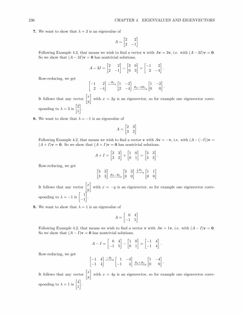
236 CHAPTER 4. EIGENVALUES AND EIGENVECTORS
7. We want to show that λ = 3 is an eigenvalue of
A =
[2 22 −1
]Following Example 4.2, that means we wish to find a vector v with Av = 3v, i.e. with (A− 3I)v = 0.So we show that (A− 3I)v = 0 has nontrivial solutions.
A− 3I =
[2 22 −1
]−[3 00 3
]=
[−1 2
2 −4
].
Row-reducing, we get [−1 2
2 −4
] −R1−−−→[1 −22 −4
]R2−2R1−−−−−→
[1 −20 0
].
It follows that any vector
[xy
]with x = 2y is an eigenvector, so for example one eigenvector corre-
sponding to λ = 3 is
[21
].
8. We want to show that λ = −1 is an eigenvalue of
A =
[2 33 2
]Following Example 4.2, that means we wish to find a vector v with Av = −v, i.e. with (A− (−I))v =(A+ I)v = 0. So we show that (A+ I)v = 0 has nontrivial solutions.
A+ I =
[2 33 2
]+
[1 00 1
]=
[3 33 3
].
Row-reducing, we get [3 33 3
]R2−R1−−−−−→
[3 30 0
] 13R1−−−→
[1 10 0
]
It follows that any vector
[xy
]with x = −y is an eigenvector, so for example one eigenvector corre-
sponding to λ = −1 is
[1−1
].
9. We want to show that λ = 1 is an eigenvalue of
A =
[0 4−1 5
]Following Example 4.2, that means we wish to find a vector v with Av = 1v, i.e. with (A− I)v = 0.So we show that (A− I)v = 0 has nontrivial solutions.
A− I =
[0 4−1 5
]−[1 00 1
]=
[−1 4−1 4
].
Row-reducing, we get [−1 4−1 4
] −R1−−−→[
1 −4−1 4
]R2+R1−−−−−→
[1 −40 0
].
It follows that any vector
[xy
]with x = 4y is an eigenvector, so for example one eigenvector corre-
sponding to λ = 1 is
[41
].
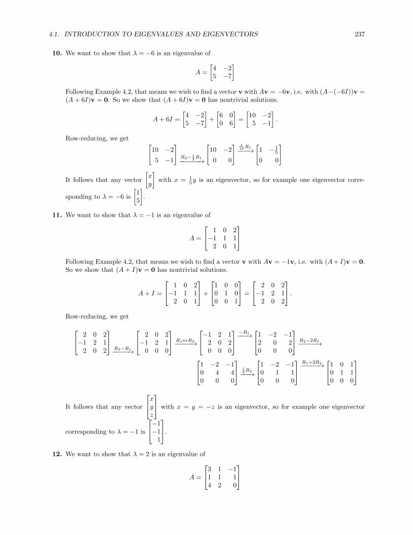
4.1. INTRODUCTION TO EIGENVALUES AND EIGENVECTORS 237
10. We want to show that λ = −6 is an eigenvalue of
A =
[4 −25 −7
]Following Example 4.2, that means we wish to find a vector v with Av = −6v, i.e. with (A−(−6I))v =(A+ 6I)v = 0. So we show that (A+ 6I)v = 0 has nontrivial solutions.
A+ 6I =
[4 −25 −7
]+
[6 00 6
]=
[10 −25 −1
].
Row-reducing, we get [10 −2
5 −1
]R2− 1
2R1−−−−−−→
[10 −2
0 0
] 110R1−−−→
[1 − 1
5
0 0
]
It follows that any vector
[xy
]with x = 1
5y is an eigenvector, so for example one eigenvector corre-
sponding to λ = −6 is
[15
].
11. We want to show that λ = −1 is an eigenvalue of
A =
1 0 2−1 1 1
2 0 1
Following Example 4.2, that means we wish to find a vector v with Av = −1v, i.e. with (A+ I)v = 0.So we show that (A+ I)v = 0 has nontrivial solutions.
A+ I =
1 0 2−1 1 1
2 0 1
+
1 0 00 1 00 0 1
=
2 0 2−1 2 1
2 0 2
.Row-reducing, we get
2 0 2−1 2 1
2 0 2
R3−R1−−−−−→
2 0 2−1 2 1
0 0 0
R1↔R2−−−−−→
−1 2 12 0 20 0 0
−R1−−−→1 −2 −1
2 0 20 0 0
R2−2R1−−−−−→
1 −2 −10 4 40 0 0
14R2−−−→
1 −2 −10 1 10 0 0
R1+2R2−−−−−→1 0 1
0 1 10 0 0
It follows that any vector
xyz
with x = y = −z is an eigenvector, so for example one eigenvector
corresponding to λ = −1 is
−1−1
1
.
12. We want to show that λ = 2 is an eigenvalue of
A =
3 1 −11 1 14 2 0

238 CHAPTER 4. EIGENVALUES AND EIGENVECTORS
Following example 4.2, that means we wish to find a vector v with Av = 2v, i.e. with (A− 2I)v = 0.So we show that (A− 2I)v = 0 has nontrivial solutions.
A− 2I =
3 1 −11 1 14 2 0
−2 0 0
0 2 00 0 2
=
1 1 −11 −1 14 2 −2
Row-reducing, we have1 1 −1
1 −1 14 2 −2
R2−R1−−−−−→R3−4R1−−−−−→
1 1 −10 −2 20 −2 2
R3−R2−−−−−→
1 1 −10 −2 20 0 0
− 12R2−−−−→
1 1 −10 1 −10 0 0
R1−R2−−−−−→1 0 0
0 1 −10 0 0
It follows that any vector[xyz
]with x = 0 and y = z is an eigenvector. Thus for example
011
is an
eigenvector for λ = 2.
13. Since A is the reflection F in the y-axis, the only vectors that F maps parallel to themselves are vectors
parallel to the x-axis (multiples of
[10
]), which are reversed (eigenvalue λ = −1) and vectors parallel
to the y-axis (multiples of
[01
]), which are sent to themselves (eigenvalue λ = 1). So λ = ±1 are the
eigenvalues of A, with eigenspaces
E−1 = span
([10
])E1 = span
([01
]).
x F HxL
e-1F He-1L=-e-1
F He1L=e1
14. The only vectors that the transformation F corresponding to A maps to themselves are vectors per-pendicular to y = x, which are reversed (so correspond to the eigenvalue λ = −1) and vectors parallelto y = x, which are sent to themselves (so correspond to the eigenvalue λ = 1. Vectors perpendicular
to y = x are multiples of
[1−1
]; vectors parallel to y = x are multiples of
[11
], so the eigenspaces are
E−1 = span
([1−1
])E1 = span
([11
]).

4.1. INTRODUCTION TO EIGENVALUES AND EIGENVECTORS 239
x
F HxLe-1
F He-1L=-e-1
F He1L=e1
15. If x is an eigenvalue of A, then Ax is a multiple of x:
Ax =
[1 00 0
] [xy
]=
[x0
].
Then clearly any vector parallel to the x-axis, i.e., of the form
[x0
], is an eigenvector for A with
eigenvalue 1. But this projection also transforms vectors parallel to the y-axis to the zero vector, since
the projection of such a vector on the x-axis is 0. So vectors of the form
[0y
]are eigenvectors for A
with eigenvalue 0. Finally, a vector of the form
[xy
]where neither x nor y is zero is not an eigenvector:
it is transformed into
[x0
], and comparing the x-coordinates shows that λ would have to be 1, while
comparing y-coordinates shows that it would have to be zero. Thus there is no such λ. So in summary,
λ = 1 is an eigenvalue with eigenspace E1 = span
([10
])λ = 0 is an eigenvalue with eigenspace E0 = span
([01
]).
16. This projection sends a vector to its projection on the given line. Then a vector parallel to the directionvector of that line will be sent to itself, since its projection on the line is the vector itself. A vectororthogonal to the direction vector of the line will be sent to the zero vector, since its projection on the
line is the zero vector. Since the direction vector is
[4535
], or
[43
], there are two eigenspaces
span
([43
]), λ = 1; span
([−3
4
]), λ = −1.
If a vector v is neither parallel to nor orthogonal to the direction vector of the line, then the projectiontransforms v to a vector parallel to the direction vector, thus not parallel to v. Thus the image of vcannot be a multiple of v. Hence the eigenvalues and eigenspaces above are the only ones.
17. Consider the action of A on a vector x =
[xy
]. If y = 0, then A multiplies x by 2, so this is an
eigenspace for λ = 2. If x = 0, then A multiplies x by 3, so this is an eigenspace for λ = 3. If neither x

240 CHAPTER 4. EIGENVALUES AND EIGENVECTORS
nor y is zero, then
[xy
]is mapped to
[2x3y
], which is not a multiple of
[xy
]. So the only eigenspaces are
span
([10
]), λ = 2; span
([01
]), λ = 3.
18. Since A rotates the plane 90◦ counterclockwise around the origin, any nonzero vector is taken toa vector orthogonal to itself. So there are no nonzero vectors that are taken to vectors parallel tothemselves (that is, to multiples of themselves). The only vector taken to a multiple of itself is thezero vector; this is not an eigenvector since eigenvectors are by definition nonzero. So this matrix hasno eigenvectors and no eigenvalues. Analytically, the matrix of A is
A =
[cos θ − sin θsin θ cos θ
]=
[0 −11 0
],
so that
Ax =
[0 −11 0
] [xy
]=
[−yx
].
If this is a multiple of the original vector, then there is a constant a such that x = −ay and y = ax.Substituting ax for y in the first equation gives x = −a2x, which is impossible unless x = 0. But thenthe second equation forces y = 0. So again we see that there are no eigenvectors.
19. Since eigenvectors x are those taken to a multiple of themselves, i.e., to a vector parallel to themselves,by A, we look for unit vectors whose image under A is in the same direction. It appears that these vec-
tors are vectors along the x and y-axes, so the eigenspaces are E1 = span
([10
])and E2 = span
([01
]).
The length of the resultant vectors in the first eigenspace appears are same length as the original vec-tor, so that λ1 = 1. The length of the resultant vectors in the second eigenspace are twice the originallength, so that λ2 = 2.
20. Since eigenvectors x are those taken to a multiple of themselves, i.e., to a vector parallel to themselves,by A, we look for unit vectors whose image under A is in the same direction. The only vectors satisfying
this criterion are those parallel to the line y = x, i.e., span
([11
]), so this is the only eigenspace. The
terminal point of the line in the direction
[11
]appears to be the point (2, 5), so that it has a length of
√29. Since the original vector is a unit vector, the eigenvalue is
√29.
21. Since eigenvectors x are those taken to a multiple of themselves, i.e., to a vector parallel to themselves,by A, we look for unit vectors whose image under A is in the same direction. The vectors parallel to
the line y = x, i.e., span
([11
])satisfy this criterion, so this is an eigenspace E1. The vectors parallel
to the line y = −x, i.e. span
([1−1
]), also satisfy this criterion, so this is another eigenspace E2. For
E1, the terminal point of the line along y = x appears to be (2, 2), so its length is 2√
2. Since theoriginal vector is a unit vector, the corresponding eigenvalue is λ1 = 2
√2. For E2, the resultant vectors
are zero length, so λ2 = 0.
22. Since eigenvectors x are those taken to a multiple of themselves, i.e., to a vector parallel to themselves,by A, we look for unit vectors whose image under A is in the same direction. There are none — everyvector is “bent” to the left by the transformation. So this transformation has no eigenvectors.
23. Using the method of Example 4.5, we wish to find solutions to the equation
0 = det(A− λI) = det
([4 −12 1
]−[λ 00 λ
])= det
[4− λ −1
2 1− λ
]= (4− λ)(1− λ)− 2 · (−1) = λ2 − 5λ+ 6 = (λ− 2)(λ− 3).

4.1. INTRODUCTION TO EIGENVALUES AND EIGENVECTORS 241
Thus the eigenvalues are 2 and 3.
To find the eigenspace corresponding to λ = 2, we must find the null space of A− 2I.
[A− 2I 0
]=
[2 −1 0
2 −1 0
]→
[1 − 1
2 0
0 0 0
]
so that eigenvectors corresponding to this eigenvalue have the form[12 tt
], or
[t2t
].
A basis for this eigenspace is given by choosing for example t = 1 to get
[12
]. As a check,
A
[12
]=
[4 −12 1
] [12
]=
[4 · 1− 1 · 22 · 1 + 1 · 2
]=
[24
]= 2
[12
].
To find the eigenspace corresponding to λ = 3, we must find the null space of A− 3I.
[A− 3I 0
]=
[1 −1 02 −2 0
]→[1 −1 00 0 0
]so that eigenvectors corresponding to this eigenvalue have the form[
tt
].
A basis for this eigenspace is given by choosing for example t = 1 to get
[11
]. As a check,
A
[11
]=
[4 −12 1
] [11
]=
[4 · 1− 1 · 12 · 1 + 1 · 1
]=
[33
]= 3
[11
]The plot below shows the effect of A on the eigenvectors
v =
[12
]w =
[11
].
v
w
2 v
3 w
1 2 3
1
2
3
4
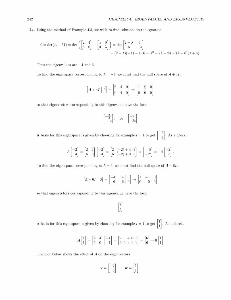
242 CHAPTER 4. EIGENVALUES AND EIGENVECTORS
24. Using the method of Example 4.5, we wish to find solutions to the equation
0 = det(A− λI) = det
([2 46 0
]−[λ 00 λ
])= det
[2− λ 4
6 −λ
]= (2− λ)(−λ)− 4 · 6 = λ2 − 2λ− 24 = (λ− 6)(λ+ 4).
Thus the eigenvalues are −4 and 6.
To find the eigenspace corresponding to λ = −4, we must find the null space of A+ 4I.
[A+ 4I 0
]=
[6 4 0
6 4 0
]→
[1 2
3 0
0 0 0
]
so that eigenvectors corresponding to this eigenvalue have the form
[− 2
3 tt
], or
[−2t
3t
]
A basis for this eigenspace is given by choosing for example t = 1 to get
[−2
3
]. As a check,
A
[−2
3
]=
[2 46 0
] [−2
3
]=
[2 · (−2) + 4 · 36 · (−2) + 0 · 3
]=
[8
−12
]= −4
[−2
3
].
To find the eigenspace corresponding to λ = 6, we must find the null space of A− 6I.
[A− 6I 0
]=
[−4 4 0
6 −6 0
]→[1 −1 00 0 0
]
so that eigenvectors corresponding to this eigenvalue have the form
[tt
]
A basis for this eigenspace is given by choosing for example t = 1 to get
[11
]. As a check,
A
[11
]=
[2 46 0
] [−1
1
]=
[2 · 1 + 4 · 16 · 1 + 0 · 1
]=
[66
]= 6
[11
]
The plot below shows the effect of A on the eigenvectors
v =
[−2
3
]w =
[11
].

4.1. INTRODUCTION TO EIGENVALUES AND EIGENVECTORS 243
v
w
-4 v
6 w
-2 2 4 6 8
-12
-10
-8
-6
-4
-2
2
4
6
25. Using the method of Example 4.5, we wish to find solutions to the equation
0 = det(A− λI) = det
([2 50 2
]−[λ 00 λ
])= det
[2− λ 5
0 2− λ
]= (2− λ)(2− λ)− 5 · 0 = (λ− 2)2
Thus the only eigenvalue is λ = 2.
To find the eigenspace corresponding to λ = 2, we must find the null space of A− 2I.[A− 2I 0
]=
[0 5 0
0 0 0
]→
[0 1 0
0 0 0
]so that eigenvectors corresponding to this eigenvalue have the form[
t0
].
A basis for this eigenspace is given by choosing for example t = 1, to get
[10
]. As a check,
A
[10
]=
[2 50 2
] [10
]=
[2 · 1 + 5 · 00 · 1 + 2 · 0
]=
[20
]= 2
[10
].
The plot below shows the effect of A on the eigenvector v =
[10
]:
v 2 v
1 2
26. Using the method of Example 4.5, we wish to find solutions to the equation
0 = det(A− λI) = det
([1 2−2 3
]−[λ 00 λ
])= det
[1− λ 2−2 3− λ
]= (1− λ)(3− λ) + 4 = λ2 − 4λ+ 7
Since this quadratic has no (real) roots, A has no (real) eigenvalues.

244 CHAPTER 4. EIGENVALUES AND EIGENVECTORS
27. Using the method of Example 4.5, we wish to find solutions to the equation
0 = det(A− λI) = det
([1 1−1 1
]−[λ 00 λ
])= det
[1− λ 1−1 1− λ
]= (1− λ)(1− λ)− 1 · (−1) = λ2 − 2λ+ 2.
Using the quadratic formula, this quadratic has roots
λ =2±√
22 − 4 · 22
=2± 2i
2= 1± i.
Thus the eigenvalues are 1 + i and 1− i.To find the eigenspace corresponding to λ = 1 + i, we must find the null space of A− (1 + i)I.
[A− (1 + i)I 0
]=
[−i 1 0−1 −i 0
]iR1−−→
[1 i 0−1 −i 0
]R2+R1−−−−−→
[1 i 00 0 0
]so that eigenvectors corresponding to this eigenvalue have the form[
−itt
].
A basis for this eigenspace is given by choosing for example t = 1, to get
[−i1
].
To find the eigenspace corresponding to λ = 1− i, we must find the null space of A− (1− i)I.
[A− (1− i)I 0
]=
[i 1 0−1 i 0
] −iR1−−−→[
1 −i 0−1 i 0
]R2+R1−−−−−→
[1 −i 00 0 0
]so that eigenvectors corresponding to this eigenvalue have the form[
itt
].
A basis for this eigenspace is given by choosing for example t = 1, to get
[i1
].
28. We wish to find solutions to the equation
0 = det(A− λI) = det
([2 −31 0
]−[λ 00 λ
])= det
[2− λ −3
1 −λ
]= (2− λ)(−λ)− (−3) · 1 = λ2 − 2λ+ 3.
Using the quadratic formula, this has roots λ = 2±√
4−4·32 = 1± i
√2, so these are the eigenvalues.
To find the eigenspace corresponding to λ = 1 + i√
2, we must find the null space of A− (1 + i√
2)I:
[A− (1 + i
√2)I 0
]=
[1− i
√2 −3 0
1 −1− i√
2 0
]R1↔R2−−−−−→[
1 −1− i√
2 0
1− i√
2 −3 0
]R2−(1−i
√2)R1−−−−−−−−−−→
[1 −1− i
√2 0
0 0 0
],
so that eigenvectors corresponding to this eigenvalue have the form[(1 + i
√2)t
t
].
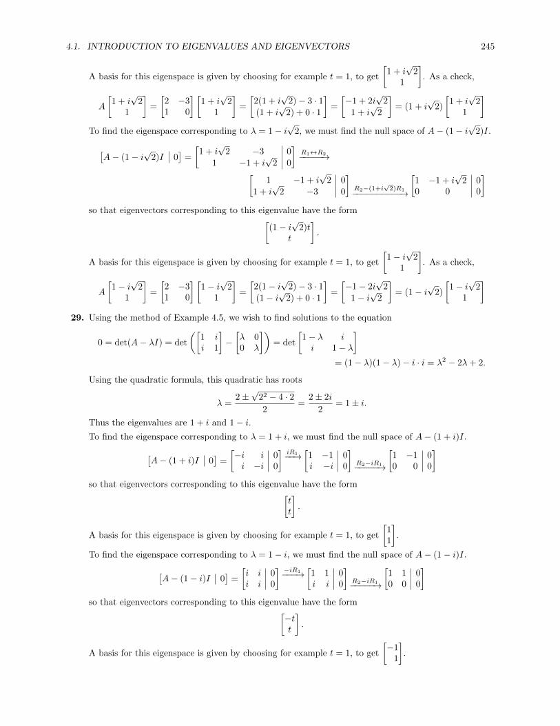
4.1. INTRODUCTION TO EIGENVALUES AND EIGENVECTORS 245
A basis for this eigenspace is given by choosing for example t = 1, to get
[1 + i
√2
1
]. As a check,
A
[1 + i
√2
1
]=
[2 −31 0
] [1 + i
√2
1
]=
[2(1 + i
√2)− 3 · 1
(1 + i√
2) + 0 · 1
]=
[−1 + 2i
√2
1 + i√
2
]= (1 + i
√2)
[1 + i
√2
1
]To find the eigenspace corresponding to λ = 1− i
√2, we must find the null space of A− (1− i
√2)I.
[A− (1− i
√2)I 0
]=
[1 + i
√2 −3 0
1 −1 + i√
2 0
]R1↔R2−−−−−→[
1 −1 + i√
2 0
1 + i√
2 −3 0
]R2−(1+i
√2)R1−−−−−−−−−−→
[1 −1 + i
√2 0
0 0 0
]so that eigenvectors corresponding to this eigenvalue have the form[
(1− i√
2)tt
].
A basis for this eigenspace is given by choosing for example t = 1, to get
[1− i
√2
1
]. As a check,
A
[1− i
√2
1
]=
[2 −31 0
] [1− i
√2
1
]=
[2(1− i
√2)− 3 · 1
(1− i√
2) + 0 · 1
]=
[−1− 2i
√2
1− i√
2
]= (1− i
√2)
[1− i
√2
1
]29. Using the method of Example 4.5, we wish to find solutions to the equation
0 = det(A− λI) = det
([1 ii 1
]−[λ 00 λ
])= det
[1− λ ii 1− λ
]= (1− λ)(1− λ)− i · i = λ2 − 2λ+ 2.
Using the quadratic formula, this quadratic has roots
λ =2±√
22 − 4 · 22
=2± 2i
2= 1± i.
Thus the eigenvalues are 1 + i and 1− i.To find the eigenspace corresponding to λ = 1 + i, we must find the null space of A− (1 + i)I.[
A− (1 + i)I 0]
=
[−i i 0i −i 0
]iR1−−→
[1 −1 0i −i 0
]R2−iR1−−−−−→
[1 −1 00 0 0
]so that eigenvectors corresponding to this eigenvalue have the form[
tt
].
A basis for this eigenspace is given by choosing for example t = 1, to get
[11
].
To find the eigenspace corresponding to λ = 1− i, we must find the null space of A− (1− i)I.[A− (1− i)I 0
]=
[i i 0i i 0
] −iR1−−−→[1 1 0i i 0
]R2−iR1−−−−−→
[1 1 00 0 0
]so that eigenvectors corresponding to this eigenvalue have the form[
−tt
].
A basis for this eigenspace is given by choosing for example t = 1, to get
[−1
1
].

246 CHAPTER 4. EIGENVALUES AND EIGENVECTORS
30. Using the method of Example 4.5, we wish to find solutions to the equation
0 = det(A− λI) = det
([0 1 + i
1− i 1
]−[λ 00 λ
])= det
[−λ 1 + i
1− i 1− λ
]= (−λ)(1− λ)− (1 + i)(1− i) = λ2 − λ− 2 = (λ− 2)(λ+ 1)
Thus the eigenvalues are 2 and −1.
To find the eigenspace corresponding to λ = 2, we must find the null space of A− 2I.
[A− 2I 0
]=
[−2 1 + i 0
1− i −1 0
]− 1
2R1−−−−→[
1 − 12 (1 + i) 0
1− i −1 0
]R2−(1−i)R1−−−−−−−−→
[1 − 1
2 (1 + i) 0
0 0 0
]
so that eigenvectors corresponding to this eigenvalue have the form[12 (1 + i)t
t
], or, clearing fractions,
[(1 + i)t
2t
].
A basis for this eigenspace is given by choosing for example t = 1, to get
[1 + i
2
].
To find the eigenspace corresponding to λ = −1, we must find the null space of A− (−I) = A+ I.
[A+ I 0
]=
[1 1 + i 0
1− i 2 0
]R2−(1−i)R1−−−−−−−−→
[1 1 + i 00 0 0
]so that eigenvectors corresponding to this eigenvalue have the form[
−(1 + i)tt
].
A basis for this eigenspace is given by choosing for example t = 1, to get
[−1− i
1
].
31. Using the method of Example 4.5, we wish to find solutions in Z3 to the equation
0 = det(A− λI) = det
([1 01 2
]−[λ 00 λ
])= det
[1− λ 0
1 2− λ
]= (1− λ)(2− λ)− 0 · 1 = (λ− 1)(λ− 2).
Thus the eigenvalues are 1 and 2.
32. Using the method of Example 4.5, we wish to find solutions in Z3 to the equation
0 = det(A− λI) = det
([2 11 2
]−[λ 00 λ
])= det
[2− λ 1
1 2− λ
]= (2− λ)(2− λ)− 1 · 1 = λ2 − 4λ+ 4− 1 = λ2 + 2λ = λ(λ+ 2) = λ(λ− 1).
Thus the eigenvalues are 0 and 1.
33. Using the method of Example 4.5, we wish to find solutions in Z5 to the equation
0 = det(A− λI) = det
([3 14 0
]−[λ 00 λ
])= det
[3− λ 1
4 −λ
]= (3− λ)(−λ)− 1 · 4 = λ2 − 3λ− 4 = λ2 + 2λ+ 1 = (λ+ 1)2 = (λ− 4)2.
Thus the only eigenvalue is 4.

4.1. INTRODUCTION TO EIGENVALUES AND EIGENVECTORS 247
34. Using the method of Example 4.5, we wish to find solutions in Z5 to the equation
0 = det(A− λI) = det
([1 44 0
]−[λ 00 λ
])= det
[1− λ 4
4 −λ
]= (1− λ)(−λ)− 4 · 4 = λ2 − λ− 16 = λ2 + 4λ+ 4 = (λ+ 2)2 = (λ− 3)2.
Thus the only eigenvalue is 3.
35. (a) To find the eigenvalues of A, find solutions to the equation
0 = det(A− λI) = det
([a bc d
]−[λ 00 λ
])= det
[a− λ bc d− λ
]= (a− λ)(d− λ)− bc = λ2 − (a+ d)λ+ (ad− bc) = λ2 − tr(A)λ+ det(A).
(b) Using the quadratic formula to find the roots of this quadratic gives
λ =tr(A)±
√(tr(A))2 − 4 det(A)
2
=a+ d±
√a2 + 2ad+ d2 − 4ad+ 4bc
2
=1
2
(a+ d±
√a2 − 2ad+ d2 + 4bc
)=
1
2
(a+ d±
√(a− d)2 + 4bc
).
(c) Let
λ1 =1
2
(a+ d+
√(a− d)2 + 4bc
), λ2 =
1
2
(a+ d−
√(a− d)2 + 4bc
)be the two eigenvalues. Then
λ1 + λ2 =1
2
(a+ d+
√(a− d)2 + 4bc
)+
1
2
(a+ d−
√(a− d)2 + 4bc
)=
1
2(a+ d+ a+ d)
= a+ d = tr(A),
λ1λ2 =
(1
2
(a+ d−
√(a− d)2 + 4bc
))(1
2
(a+ d−
√(a− d)2 + 4bc
))=
1
4
((a+ d)2 −
((a− d)2 + 4bc
))=
1
4(a2 + 2ad+ d2 − a2 + 2ad− d2 − 4bc)
=1
4(4ad− 4bc) = det(A).
36. A quadratic equation will have two distinct real roots when its discriminant (the quantity under thesquare root sign in the quadratic formula) is positive, one real root when it is zero, and no real rootswhen it is negative. In Exercise 35, the discriminant is (a− d)2 + 4bc.
(a) For A to have to distinct real eigenvalues, we must have (a− d)2 + 4bc > 0.
(b) For A to have a single real eigenvalue, it must be the case that (a − d)2 + 4bc = 0, so that(a−d)2 = −4bc. Note that this implies that either a = d and at least one of b or c is zero, or thata 6= d and either b or c, but not both, is negative.
(c) For A to have no real eigenvalues, we must have (a− c)2 + 4bc < 0.

248 CHAPTER 4. EIGENVALUES AND EIGENVECTORS
37. From Exercise 35, since c = 0, the eigenvalues are
1
2
(a+ d±
√(a− d)2 + 4b · 0
)=
1
2(a+ d± |a− d|)
=
{1
2(a+ d+ a− d),
1
2(a+ d+ d− a)
}= {a, d}.
To find the eigenspace corresponding to λ = a, we must find the null space of A− aI.
[A− aI 0
]=
[0 b 00 d− a 0
].
If b = 0 and a = d, then this is the zero matrix, so that any vector is an eigenvector; a basis for theeigenspace is {[
10
],
[01
]}.
The reason for this is that under these conditions, the matrix A is a multiple of the identity matrix, soit simply stretches any vector by a factor of a = d. Otherwise, either b 6= 0 or d− a 6= 0, so the abovematrix row-reduces to [
0 1 00 0 0
]so that eigenvectors corresponding to this eigenvalue have the form[
t0
].
A basis for this eigenspace is given by choosing for example t = 1, to get
[10
]. As a check,
A
[10
]=
[a · 1 + b · 00 · 1 + d · 0
]=
[a0
]= a
[10
].
To find the eigenspace corresponding to λ = d, we must find the null space of A− dI.
[A− dI 0
]=
[a− d b 0
0 0 0
].
If b = 0 and a = d, then this is again the zero matrix, which we dealt with above. Otherwise, eitherb 6= 0 or d− a 6= 0, so that eigenvectors corresponding to this eigenvalue have the form[
−bt(a− d)t
], or
[bt
(d− a)t
].
A basis for this eigenspace is given by choosing for example t = 1, to get
[b
d− a
]. As a check,
A
[b
d− a
]=
[a · b+ b · (d− a)0 · b+ d · (d− a)
]=
[bd
d(d− a)
]= d
[b
d− a
].
38. Using the method of Example 4.5, we wish to find solutions to the equation
0 = det(A− λI) = det
([a b−b a
]−[λ 00 λ
])= det
[a− λ b−b a− λ
]= (a− λ)(a− λ)− 4 · (−b) = λ2 − 2aλ+ (a2 + 4b).

4.1. INTRODUCTION TO EIGENVALUES AND EIGENVECTORS 249
Using Exercise 35, the eigenvalues are
1
2
(a+ a±
√(a− a)2 + 4b · (−b)
)= a± 1
2
√−4b2 = a± bi.
To find the eigenspace corresponding to λ = a+ bi, we must find the null space of A− (a+ bi)I.
[A− (a+ bi)I 0
]=
[−bi b 0−b −bi 0
].
If b = 0 then this is the zero matrix, so that any vector is an eigenvector; a basis for the eigenspace is{[10
],
[01
]}.
The reason for this is that under these conditions, the matrix A is a times the identity matrix, so itsimply stretches any vector by a factor of a. Otherwise, b 6= 0, so we can row-reduce the matrix:[
−bi b 0−b −bi 0
] 1b iR1−−−→
[1 i 0−b −bi 0
]R2+bR1−−−−−→
[1 i 00 0 0
].
Thus eigenvectors corresponding to this eigenvalue have the form[−itt
]=
[tit
].
A basis for this eigenspace is given by choosing for example t = 1, to get
[1i
]. As a check,
A
[1i
]=
[a+ bi−b+ ai
]= (a+ bi)
[1i
].
To find the eigenspace corresponding to λ = a− bi, we must find the null space of A− (a− bi)I.
[A− (a− bi)I 0
]=
[bi b 0−b bi 0
].
If b = 0 then this is the zero matrix, which we dealt with above. Otherwise, b 6= 0, so we can row-reducethe matrix: [
bi b 0−b bi 0
] − 1b iR1−−−−→
[1 −i 0−b bi 0
]R2+bR1−−−−−→
[1 −i 00 0 0
].
Thus eigenvectors corresponding to this eigenvalue have the form[itt
].
A basis for this eigenspace is given by choosing for example t = 1, to get
[i1
]. As a check,
A
[i1
]=
[ai+ b−bi+ a
]=
[b+ aia− bi
]= (a− bi)
[i1
].
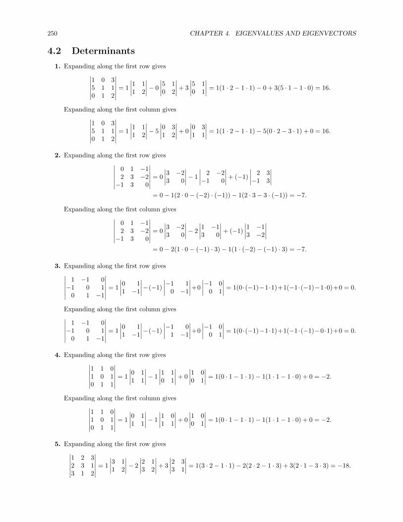
250 CHAPTER 4. EIGENVALUES AND EIGENVECTORS
4.2 Determinants
1. Expanding along the first row gives∣∣∣∣∣∣1 0 35 1 10 1 2
∣∣∣∣∣∣ = 1
∣∣∣∣1 11 2
∣∣∣∣− 0
∣∣∣∣5 10 2
∣∣∣∣+ 3
∣∣∣∣5 10 1
∣∣∣∣ = 1(1 · 2− 1 · 1)− 0 + 3(5 · 1− 1 · 0) = 16.
Expanding along the first column gives∣∣∣∣∣∣1 0 35 1 10 1 2
∣∣∣∣∣∣ = 1
∣∣∣∣1 11 2
∣∣∣∣− 5
∣∣∣∣0 31 2
∣∣∣∣+ 0
∣∣∣∣0 31 1
∣∣∣∣ = 1(1 · 2− 1 · 1)− 5(0 · 2− 3 · 1) + 0 = 16.
2. Expanding along the first row gives∣∣∣∣∣∣0 1 −12 3 −2−1 3 0
∣∣∣∣∣∣ = 0
∣∣∣∣3 −23 0
∣∣∣∣− 1
∣∣∣∣ 2 −2−1 0
∣∣∣∣+ (−1)
∣∣∣∣ 2 3−1 3
∣∣∣∣= 0− 1(2 · 0− (−2) · (−1))− 1(2 · 3− 3 · (−1)) = −7.
Expanding along the first column gives∣∣∣∣∣∣0 1 −12 3 −2−1 3 0
∣∣∣∣∣∣ = 0
∣∣∣∣3 −23 0
∣∣∣∣− 2
∣∣∣∣1 −13 0
∣∣∣∣+ (−1)
∣∣∣∣1 −13 −2
∣∣∣∣= 0− 2(1 · 0− (−1) · 3)− 1(1 · (−2)− (−1) · 3) = −7.
3. Expanding along the first row gives∣∣∣∣∣∣1 −1 0−1 0 1
0 1 −1
∣∣∣∣∣∣ = 1
∣∣∣∣0 11 −1
∣∣∣∣−(−1)
∣∣∣∣−1 10 −1
∣∣∣∣+0
∣∣∣∣−1 00 1
∣∣∣∣ = 1(0 ·(−1)−1 ·1)+1(−1 ·(−1)−1 ·0)+0 = 0.
Expanding along the first column gives∣∣∣∣∣∣1 −1 0−1 0 1
0 1 −1
∣∣∣∣∣∣ = 1
∣∣∣∣0 11 −1
∣∣∣∣−(−1)
∣∣∣∣−1 01 −1
∣∣∣∣+0
∣∣∣∣−1 00 1
∣∣∣∣ = 1(0 ·(−1)−1 ·1)+1(−1 ·(−1)−0 ·1)+0 = 0.
4. Expanding along the first row gives∣∣∣∣∣∣1 1 01 0 10 1 1
∣∣∣∣∣∣ = 1
∣∣∣∣0 11 1
∣∣∣∣− 1
∣∣∣∣1 10 1
∣∣∣∣+ 0
∣∣∣∣1 00 1
∣∣∣∣ = 1(0 · 1− 1 · 1)− 1(1 · 1− 1 · 0) + 0 = −2.
Expanding along the first column gives∣∣∣∣∣∣1 1 01 0 10 1 1
∣∣∣∣∣∣ = 1
∣∣∣∣0 11 1
∣∣∣∣− 1
∣∣∣∣1 01 1
∣∣∣∣+ 0
∣∣∣∣1 00 1
∣∣∣∣ = 1(0 · 1− 1 · 1)− 1(1 · 1− 1 · 0) + 0 = −2.
5. Expanding along the first row gives∣∣∣∣∣∣1 2 32 3 13 1 2
∣∣∣∣∣∣ = 1
∣∣∣∣3 11 2
∣∣∣∣− 2
∣∣∣∣2 13 2
∣∣∣∣+ 3
∣∣∣∣2 33 1
∣∣∣∣ = 1(3 · 2− 1 · 1)− 2(2 · 2− 1 · 3) + 3(2 · 1− 3 · 3) = −18.

4.2. DETERMINANTS 251
Expanding along the first column gives∣∣∣∣∣∣1 2 32 3 13 1 2
∣∣∣∣∣∣ = 1
∣∣∣∣3 11 2
∣∣∣∣− 2
∣∣∣∣2 13 2
∣∣∣∣+ 3
∣∣∣∣2 33 1
∣∣∣∣ = 1(3 · 2− 1 · 1)− 2(2 · 2− 1 · 3) + 3(2 · 1− 3 · 3) = −18.
6. Expanding along the first row gives∣∣∣∣∣∣1 2 34 5 67 8 9
∣∣∣∣∣∣ = 1
∣∣∣∣5 68 9
∣∣∣∣− 2
∣∣∣∣4 67 9
∣∣∣∣+ 3
∣∣∣∣4 57 8
∣∣∣∣ = 1(5 · 9− 6 · 8)− 2(4 · 9− 6 · 7) + 3(4 · 8− 5 · 7) = 0.
Expanding along the first column gives∣∣∣∣∣∣1 2 34 5 67 8 9
∣∣∣∣∣∣ = 1
∣∣∣∣5 68 9
∣∣∣∣− 4
∣∣∣∣2 38 9
∣∣∣∣+ 7
∣∣∣∣2 35 6
∣∣∣∣ = 1(5 · 9− 6 · 8)− 4(2 · 9− 3 · 8) + 7(2 · 6− 3 · 5) = 0.
7. Noting the pair of zeros in the third row, use cofactor expansion along the third row to get∣∣∣∣∣∣5 2 2−1 1 2
3 0 0
∣∣∣∣∣∣ = 3
∣∣∣∣2 21 2
∣∣∣∣− 0
∣∣∣∣ 5 2−1 2
∣∣∣∣+ 0
∣∣∣∣ 5 2−1 1
∣∣∣∣ = 3(2 · 2− 2 · 1)− 0 + 0 = 6.
8. Noting the zero in the second row, use cofactor expansion along the second row to get∣∣∣∣∣∣1 1 −12 0 13 −2 1
∣∣∣∣∣∣ = −2
∣∣∣∣ 1 −1−2 1
∣∣∣∣− 1
∣∣∣∣1 13 −2
∣∣∣∣ = −2(1 · 1− (−1) · (−2))− 1(1 · (−2)− 1 · 3) = 7.
9. Noting the zero in the bottom right, use the third row, since the multipliers there are smaller:∣∣∣∣∣∣−4 1 3
2 −2 41 −1 0
∣∣∣∣∣∣ = 1
∣∣∣∣ 1 3−2 4
∣∣∣∣− (−1)
∣∣∣∣−4 32 4
∣∣∣∣ = 1(1 · 4− 3 · (−2)) + 1(−4 · 4− 3 · 2) = −12.
10. Noting that the first column has only one nonzero entry, we expand along the first column:∣∣∣∣∣∣cos θ sin θ tan θ
0 cos θ − sin θ0 sin θ cos θ
∣∣∣∣∣∣ = cos θ(cos θ · cos θ − (− sin θ) · sin θ) = cos θ(cos2 θ + sin2 θ) = cos θ.
11. Use the first column:∣∣∣∣∣∣a b 00 a ba 0 b
∣∣∣∣∣∣ = a
∣∣∣∣a b0 b
∣∣∣∣+ a
∣∣∣∣b 0a b
∣∣∣∣ = a(a · b− b · 0) + a(b · b− 0 · a) = a2b+ ab2.
12. Use the first row (other choices are equally easy):∣∣∣∣∣∣0 a 0b c d0 e 0
∣∣∣∣∣∣ = −a∣∣∣∣b d0 0
∣∣∣∣ = −a(b · 0− d · 0) = 0.

252 CHAPTER 4. EIGENVALUES AND EIGENVECTORS
13. Use the third row, since it contains only one nonzero entry:∣∣∣∣∣∣∣∣1 −1 0 32 5 2 60 1 0 01 4 2 1
∣∣∣∣∣∣∣∣ = (−1)3+2 · 1
∣∣∣∣∣∣1 0 32 2 61 2 1
∣∣∣∣∣∣ = −
∣∣∣∣∣∣1 0 32 2 61 2 1
∣∣∣∣∣∣ .To compute this determinant, use cofactor expansion along the first row:
−
∣∣∣∣∣∣1 0 32 2 61 2 1
∣∣∣∣∣∣ = −1
∣∣∣∣2 62 1
∣∣∣∣− 3
∣∣∣∣2 21 2
∣∣∣∣ = −1(2 · 1− 6 · 2)− 3(2 · 2− 2 · 1) = 4.
14. Noting that the second column has only one nonzero entry, we expand along that column. The nonzeroentry is in row 3, column 2, so it gets a minus sign, since (−1)3+2 = −1:∣∣∣∣∣∣∣∣
2 0 3 −11 0 2 20 −1 1 42 0 1 −3
∣∣∣∣∣∣∣∣ = −(−1)
∣∣∣∣∣∣2 3 −11 2 22 1 −3
∣∣∣∣∣∣ =
∣∣∣∣∣∣2 3 −11 2 22 1 −3
∣∣∣∣∣∣ .To evaluate the remaining determinant, we use expansion along the first row:∣∣∣∣∣∣
2 3 −11 2 22 1 −3
∣∣∣∣∣∣ = 2
∣∣∣∣2 21 −3
∣∣∣∣− 3
∣∣∣∣1 22 −3
∣∣∣∣− 1
∣∣∣∣1 22 1
∣∣∣∣= 2(2 · (−3)− 2 · 1)− 3(1 · (−3)− 2 · 2)− 1(1 · 1− 2 · 2) = 8.
15. Expand along the first row: ∣∣∣∣∣∣∣∣0 0 0 a0 0 b c0 d e fg h i j
∣∣∣∣∣∣∣∣ = −a
∣∣∣∣∣∣0 0 b0 d eg h i
∣∣∣∣∣∣ .Now expand along the first row again:
−a
∣∣∣∣∣∣0 0 b0 d eg h i
∣∣∣∣∣∣ = −ab∣∣∣∣0 dg h
∣∣∣∣ = −ab(0 · h− dg) = abdg.
16. Using the method of Example 4.9, we get
105 48 72∣∣∣∣∣∣1 2 34 5 67 8 9
∣∣∣∣∣∣1 24 57 8
45 84 96
so that the determinant is −(105 + 48 + 72) + (45 + 84 + 96) = 0.
17. Using the method of Example 4.9,
0 −2 2∣∣∣∣∣∣1 1 −12 0 13 −2 1
∣∣∣∣∣∣1 12 03 −2
0 3 4
so that the determinant is −(0 + (−2) + 2) + (0 + 3 + 4) = 7.

4.2. DETERMINANTS 253
18. Using the method of Example 4.9, we get
0 0 0∣∣∣∣∣∣a b 00 a ba 0 b
∣∣∣∣∣∣a b0 aa 0
a2b ab2 0
so that the determinant is −(0 + 0 + 0) + (a2b+ ab2 + 0) = a2b+ ab2.
19. Consider (2) in the text. The three upward-pointing diagonals have product a31a22a13, a32a23a11, anda33a21a12, while the downward-pointing diagonals have product a11a22a33, a12a23a31, and a13a21a32,so the determinant by that method is
detA = −(a31a22a13 + a32a23a11 + a33a21a12) + (a11a22a33 + a12a23a31 + a13a21a32).
Expanding along the first row gives
detA = a11
∣∣∣∣a22 a23
a32 a33
∣∣∣∣− a12
∣∣∣∣a21 a23
a31 a33
∣∣∣∣+ a13
∣∣∣∣a21 a22
a31 a32
∣∣∣∣= a11a22a33 − a11a32a23 − a12a21a33 + a12a23a31 + a13a21a32 − a13a22a31,
which, after rearranging, is the same as the first answer.
20. Consider the 2× 2 matrix A =
[a11 a12
a21 a22
]. Then
C11 = (−1)1+1 det[a22] = a22, C12 = (−1)1+2 det[a21] = −a21,
so that from definition (4)
detA =
2∑j=1
a1jC1j = a11C11 + a12C12 = a11a12 + a12 · (−a21) = a11a22 − a12a21,
which agrees with the definition of a 2× 2 determinant.
21. If A is lower triangular, then AT is upper triangular. Since by Theorem 4.10 detA = detAT , if weprove the result for upper triangular matrices, we will have proven it for lower triangular matrices aswell. So assume A is upper triangular. The basis for the induction is the case n = 1, where A = [a11]and detA = a11, which is clearly the “product” of the entries on the diagonal. Now assume that thestatement holds for n×n upper triangular matrices, and let A be an (n+ 1)× (n+ 1) upper triangularmatrix. Using cofactor expansion along the last row, we get
detA = (−1)(n+1)+(n+1)an+1,n+1An+1,n+1 = an+1,n+1An+1,n+1.
But An+1,n+1 is an n×n upper triangular matrix with diagonal entries a1, a2, . . . , an, so applying theinductive hypothesis we get
detA = an+1,n+1An+1,n+1 = an+1,n+1(a1a2 · · · an) = a1a2 · · · anan+1,
proving the result for (n+ 1)× (n+ 1) matrices. So by induction, the statement is true for all n ≥ 1.
22. Row-reducing the matrix in Exercise 1, and modifying the determinant as required by Theorem 4.3,gives ∣∣∣∣∣∣
1 0 35 1 10 1 2
∣∣∣∣∣∣ R2−5R1−−−−−→
∣∣∣∣∣∣1 0 30 1 −140 1 2
∣∣∣∣∣∣ R3−R2−−−−−→
∣∣∣∣∣∣1 0 30 1 −140 0 16
∣∣∣∣∣∣Note that we did not introduce any factors in front of the determinant since all of the row operationswere of the form Ri + kRj , which does not change the determinant. The final determinant is easy toevaluate since the matrix is upper triangular; the determinant of the original matrix is 1 · 1 · 16 = 16.
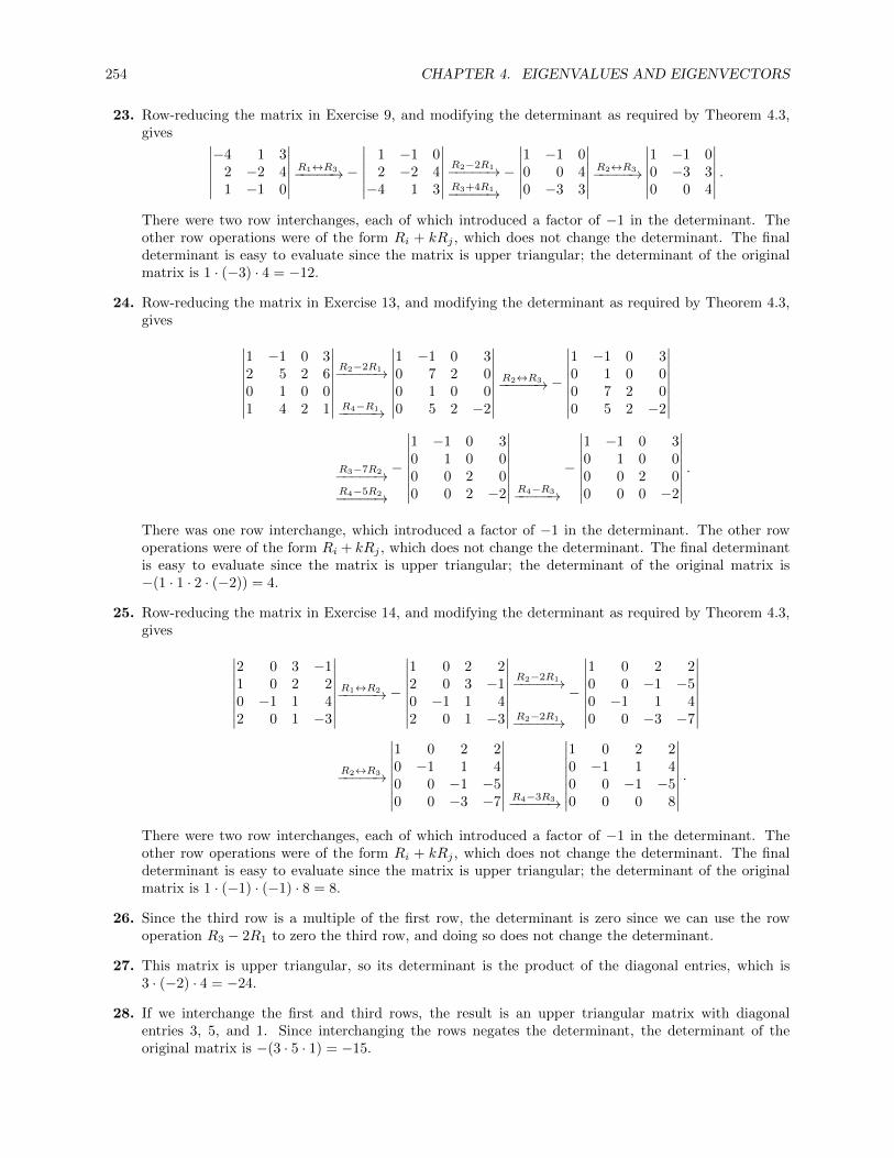
254 CHAPTER 4. EIGENVALUES AND EIGENVECTORS
23. Row-reducing the matrix in Exercise 9, and modifying the determinant as required by Theorem 4.3,gives ∣∣∣∣∣∣
−4 1 32 −2 41 −1 0
∣∣∣∣∣∣ R1↔R3−−−−−→−
∣∣∣∣∣∣1 −1 02 −2 4−4 1 3
∣∣∣∣∣∣ R2−2R1−−−−−→R3+4R1−−−−−→
−
∣∣∣∣∣∣1 −1 00 0 40 −3 3
∣∣∣∣∣∣ R2↔R3−−−−−→
∣∣∣∣∣∣1 −1 00 −3 30 0 4
∣∣∣∣∣∣ .There were two row interchanges, each of which introduced a factor of −1 in the determinant. Theother row operations were of the form Ri + kRj , which does not change the determinant. The finaldeterminant is easy to evaluate since the matrix is upper triangular; the determinant of the originalmatrix is 1 · (−3) · 4 = −12.
24. Row-reducing the matrix in Exercise 13, and modifying the determinant as required by Theorem 4.3,gives ∣∣∣∣∣∣∣∣
1 −1 0 32 5 2 60 1 0 01 4 2 1
∣∣∣∣∣∣∣∣R2−2R1−−−−−→
R4−R1−−−−−→
∣∣∣∣∣∣∣∣1 −1 0 30 7 2 00 1 0 00 5 2 −2
∣∣∣∣∣∣∣∣R2↔R3−−−−−→−
∣∣∣∣∣∣∣∣1 −1 0 30 1 0 00 7 2 00 5 2 −2
∣∣∣∣∣∣∣∣R3−7R2−−−−−→R4−5R2−−−−−→
−
∣∣∣∣∣∣∣∣1 −1 0 30 1 0 00 0 2 00 0 2 −2
∣∣∣∣∣∣∣∣ R4−R3−−−−−→
−
∣∣∣∣∣∣∣∣1 −1 0 30 1 0 00 0 2 00 0 0 −2
∣∣∣∣∣∣∣∣ .There was one row interchange, which introduced a factor of −1 in the determinant. The other rowoperations were of the form Ri + kRj , which does not change the determinant. The final determinantis easy to evaluate since the matrix is upper triangular; the determinant of the original matrix is−(1 · 1 · 2 · (−2)) = 4.
25. Row-reducing the matrix in Exercise 14, and modifying the determinant as required by Theorem 4.3,gives ∣∣∣∣∣∣∣∣
2 0 3 −11 0 2 20 −1 1 42 0 1 −3
∣∣∣∣∣∣∣∣R1↔R2−−−−−→−
∣∣∣∣∣∣∣∣1 0 2 22 0 3 −10 −1 1 42 0 1 −3
∣∣∣∣∣∣∣∣R2−2R1−−−−−→
R2−2R1−−−−−→
−
∣∣∣∣∣∣∣∣1 0 2 20 0 −1 −50 −1 1 40 0 −3 −7
∣∣∣∣∣∣∣∣R2↔R3−−−−−→
∣∣∣∣∣∣∣∣1 0 2 20 −1 1 40 0 −1 −50 0 −3 −7
∣∣∣∣∣∣∣∣ R4−3R3−−−−−→
∣∣∣∣∣∣∣∣1 0 2 20 −1 1 40 0 −1 −50 0 0 8
∣∣∣∣∣∣∣∣ .There were two row interchanges, each of which introduced a factor of −1 in the determinant. Theother row operations were of the form Ri + kRj , which does not change the determinant. The finaldeterminant is easy to evaluate since the matrix is upper triangular; the determinant of the originalmatrix is 1 · (−1) · (−1) · 8 = 8.
26. Since the third row is a multiple of the first row, the determinant is zero since we can use the rowoperation R3 − 2R1 to zero the third row, and doing so does not change the determinant.
27. This matrix is upper triangular, so its determinant is the product of the diagonal entries, which is3 · (−2) · 4 = −24.
28. If we interchange the first and third rows, the result is an upper triangular matrix with diagonalentries 3, 5, and 1. Since interchanging the rows negates the determinant, the determinant of theoriginal matrix is −(3 · 5 · 1) = −15.

4.2. DETERMINANTS 255
29. The third column is −2 times the first column, so the columns are not linearly independent and thusthe matrix does not have rank 3, so is not invertible. By Theorem 4.6, its determinant is zero.
30. Since the third row is the sum of the first and second rows, the rows are not linearly independent andthus the matrix does not have rank 3, so is not invertible. By Theorem 4.6, its determinant is zero.
31. Since the first column is the sum of the second and third columns, the columns are not linearlyindependent and thus the matrix does not have rank 3, so is not invertible. By Theorem 4.6, itsdeterminant is zero.
32. Interchanging the second and third rows gives the identity matrix, which has determinant 1. Sinceinterchanging the rows introduces a minus sign, the determinant of the original matrix is −1.
33. Interchange the first and second rows, and also the third and fourth rows, to give a diagonal matrix withdiagonal entries −3, 2, 1, and 4. Performing two row interchanges does not change the determinant,so the determinant of the original matrix is −3 · 2 · 1 · 4 = −24.
34. The sum of the first and second rows is equal to the sum of the third and fourth rows, so the rows arenot linearly independent and thus the matrix does not have rank 4, so is not invertible. By Theorem4.6, its determinant is zero.
35. This matrix results from the original matrix by multiplying the first row by 2, so its determinant is2 · 4 = 8.
36. This matrix results from the original matrix by multiplying the first column by 2, the second columnby 1
3 , and the third column by −1. Thus the determinant of this matrix is 2 · 13 · (−1) = − 2
3 times theoriginal determinant, so its value is − 2
3 · 4 = − 83 .
37. This matrix results from the original matrix by interchanging the first and second rows. This multipliesthe determinant by −1, so the determinant of this matrix is −4.
38. This matrix results from the original matrix by subtracting the third column from the first. Thisoperation does not change the determinant, so the determinant of this matrix is also 4.
39. This matrix results from the original matrix by exchanging the first and third columns (which multipliesthe determinant by −1) and then multiplying the first column by 2 (which multiplies the determinantby 2). So the determinant of this matrix is 2 · (−1) · 4 = −8.
40. To get from the original matrix to this one, row 2 was multiplied by 3, and then twice row 3 wasadded to each of rows 1 and 2. The first of these operations multiplies the determinant by 3, while theadditions do not change the determinant. Thus the determinant of this matrix is 3 · 4 = 12.
41. Suppose first that A has a zero row, say the ith row is zero. Using cofactor expansion along that rowgives
detA =
n∑j=1
aijCij =
n∑j=1
0Cij = 0,
so the determinant is zero. Similarly, if A has a zero column, say the jth column, then using cofactorexpansion along that column gives
detA =
n∑i=1
aijCij =
n∑i=1
0Cij = 0,
and again the determinant is zero. Alternatively, the column case can be proved from the row case bynoting that if A has a zero column, then AT has a zero row, and detA = detAT by Theorem 4.10.

256 CHAPTER 4. EIGENVALUES AND EIGENVECTORS
42. Dealing first with rows, we want to show that if ARi+kRj−−−−−→ B where i 6= j then detB = detA. Let Ai
be the ith row of A. Then
B =
A1
A2
...Ai + kAj
...An
; let C =
A1
A2
...kAj
...An
.
Then A, B, and C are identical except that the ith row of B is the sum of the ith rows of A and C,so that by part (a), detB = detA+ detC. However, since i 6= j, the ith row of C, which is kAj , is amultiple of the jth row, which is Aj . By Theorem 4.3(d), multiplying the jth row by k multiplies thedeterminant of C by k. However, the result is a matrix with two identical rows; both the ith and jth
rows are kAj . So detC = 0 by Theorem 4.3(c). Hence detB = detA as desired.
If instead ACi+kCj−−−−−→ B where i 6= j, then AT
Ri+kRj−−−−−→ BT , so that by the first part and Theorem 4.10
detA = detAT = detBT = detB.
43. If E interchanges two rows, then detE = −1 by Theorem 4.4. Also, EB is the same as B but with tworows interchanged, so by Theorem 4.3(b), det(EB) = −detB = det(E) det(B). Next, if E results frommultiplying a row by a constant k, then detE = k by Theorem 4.4. But EB is the same as B except thatone row has been multiplied by k, so that by Theorem 4.3(d), det(EB) = k det(B) = det(E) det(B).Finally, if E results from adding a multiple of one row to another row, then detE = 1 by Theorem 4.4.But in this case EB is obtained from B by adding a multiple of one row to another, so by Theorem4.3(f), det(EB) = det(B) = det(E) det(B).
44. Let the row vectors of A be A1, A2, . . . ,An. Then the row vectors of kA are kA1, kA2, . . . , kAn.Using Theorem 4.3(d) n times,
det(kA) =
∣∣∣∣∣∣∣∣∣kA1
kA2
...kAn
∣∣∣∣∣∣∣∣∣ = k
∣∣∣∣∣∣∣∣∣A1
kA2
...kAn
∣∣∣∣∣∣∣∣∣ = k2
∣∣∣∣∣∣∣∣∣A1
A2
...kAn
∣∣∣∣∣∣∣∣∣ = · · · = kn
∣∣∣∣∣∣∣∣∣A1
A2
...An
∣∣∣∣∣∣∣∣∣ = kn detA.
45. By Theorem 4.6, A is invertible if and only if detA 6= 0. To find detA, expand along the first column:
detA = k
∣∣∣∣k + 1 1−8 k − 1
∣∣∣∣+ k
∣∣∣∣ −k 3k + 1 1
∣∣∣∣= k((k + 1)(k − 1)− 1 · (−8)) + k(−k · 1− 3(k + 1)) = k3 − 4k2 + 4k = k(k − 2)2.
Thus detA = 0 when k = 0 or k = 2, so A is invertible for all k except k = 0 and k = 2.
46. By Theorem 4.6, A is invertible if and only if detA 6= 0. To find detA, expand along the first row:∣∣∣∣∣∣k k 0k2 2 k0 k k
∣∣∣∣∣∣ = k
∣∣∣∣2 kk k
∣∣∣∣− k ∣∣∣∣k2 k0 k
∣∣∣∣= k(2k − k2)− k(k3 − 0) = k(2k − k2 − k3) = k2(2− k − k2) = −k2(k + 2)(k − 1).
Since the matrix is invertible precisely when its determinant is nonzero, and since the determinant iszero when k = 0, k = 1, or k = −2, we see that the matrix is invertible for all values of k except for 0,1, and −2.
47. By Theorem 4.8, det(AB) = det(A) det(B) = 3 · (−2) = −6.

4.2. DETERMINANTS 257
48. By Theorem 4.8, det(A2) = det(A) det(A) = 3 · 3 = 9.
49. By Theorem 4.9, det(B−1) = 1det(B) , so that by Theorem 4.8
det(B−1A) = det(B−1) det(A) =det(A)
det(B)= −3
2.
50. By Theorem 4.7, det(2A) = 2n det(A) = 3 · 2n.
51. By Theorem 4.10, det(BT ) = det(B), so that by Theorem 4.7, det(3BT ) = 3n det(BT ) = −2 · 3n.
52. By Theorem 4.10, det(AT ) = det(A), so that by Theorem 4.8,
det(AAT ) = det(A) det(AT ) = det(A)2 = 9.
53. By Theorem 4.8, det(AB) = det(A) det(B) = det(B) det(A) = det(BA).
54. If B is invertible, then det(B) 6= 0 and det(B−1) = 1det(B) , so that using Theorem 4.8
det(B−1AB) = det(B−1(AB)) = det(B−1) det(AB)
= det(B−1) det(A) det(B) =1
det(B)det(A) det(B) = det(A).
55. If A2 = A, then det(A2) = det(A). But det(A2) = det(A) det(A) = det(A)2, so that det(A) = det(A)2.Thus det(A) is either 0 or 1.
56. We first show that Theorem 4.8 extends to prove that if m ≥ 1, then det(Am) = det(A)m. The casem = 1 is obvious, and m = 2 is Theorem 4.8. Now assume the statement is true for m = k. Thenusing Theorem 4.8 and the truth of the statement for m = k,
det(Ak+1) = det(AAk) = det(A) det(Ak) = det(A) det(A)k = det(A)k+1.
So the statement holds for all m ≥ 1. Now, if Am = O, then det(Am) = det(A)m = det(O) = 0, sothat det(A) = 0.
57. The coefficient matrix and constant vector are
A =
[1 11 −1
], b =
[12
].
To apply Cramer’s Rule, we compute
detA =
∣∣∣∣1 11 −1
∣∣∣∣ = −2
detA1(b) =
∣∣∣∣1 12 −1
∣∣∣∣ = −3
detA2(b) =
∣∣∣∣1 11 2
∣∣∣∣ = 1.
Then by Cramer’s Rule,
x =detA1(b)
detA=
3
2, y =
detA2(b)
detA= −1
2.
58. The coefficient matrix and constant vector are
A =
[2 −11 3
], b =
[5−1
].

258 CHAPTER 4. EIGENVALUES AND EIGENVECTORS
To apply Cramer’s Rule, we compute
detA =
∣∣∣∣2 −11 3
∣∣∣∣ = 7
detA1(b) =
∣∣∣∣ 5 −1−1 3
∣∣∣∣ = 14
detA2(b) =
∣∣∣∣2 51 −1
∣∣∣∣ = −7.
Then by Cramer’s Rule,
x =detA1(b)
detA= 2, y =
detA2(b)
detA= −1.
59. The coefficient matrix and constant vector are
A =
2 1 30 1 10 0 1
, b =
111
.To apply Cramer’s Rule, we compute
detA =
∣∣∣∣∣∣2 1 30 1 10 0 1
∣∣∣∣∣∣ = 2 · 1 · 1 = 2
detA1(b) =
∣∣∣∣∣∣1 1 31 1 11 0 1
∣∣∣∣∣∣ = 1
∣∣∣∣1 31 1
∣∣∣∣+ 1
∣∣∣∣1 11 1
∣∣∣∣ = −2
detA2(b) =
∣∣∣∣∣∣2 1 30 1 10 1 1
∣∣∣∣∣∣ = 2
∣∣∣∣1 11 1
∣∣∣∣ = 0
detA3(b) =
∣∣∣∣∣∣2 1 10 1 10 0 1
∣∣∣∣∣∣ = 2
∣∣∣∣1 10 1
∣∣∣∣ = 2.
Then by Cramer’s Rule,
x =detA1(b)
detA= −1, y =
detA2(b)
detA= 0, z =
detA3(b)
detA= 1.
60. The coefficient matrix and constant vector are
A =
1 1 −11 1 11 −1 0
, b =
123
.To apply Cramer’s Rule, we compute
detA =
∣∣∣∣∣∣1 1 −11 1 11 −1 0
∣∣∣∣∣∣ = 1
∣∣∣∣1 −11 1
∣∣∣∣− (−1)
∣∣∣∣1 −11 1
∣∣∣∣ = 4
detA1(b) =
∣∣∣∣∣∣1 1 −12 1 13 −1 0
∣∣∣∣∣∣ = 3
∣∣∣∣1 −11 1
∣∣∣∣− (−1)
∣∣∣∣1 −12 1
∣∣∣∣ = 9
detA2(b) =
∣∣∣∣∣∣1 1 −11 2 11 3 0
∣∣∣∣∣∣ = 1
∣∣∣∣1 −12 1
∣∣∣∣− 3
∣∣∣∣1 −11 1
∣∣∣∣ = −3
detA3(b) =
∣∣∣∣∣∣1 1 11 1 21 −1 3
∣∣∣∣∣∣ = 1
∣∣∣∣ 1 2−1 3
∣∣∣∣− 1
∣∣∣∣1 21 3
∣∣∣∣+ 1
∣∣∣∣1 11 −1
∣∣∣∣ = 2.
4.2. DETERMINANTS 259
Then by Cramer’s Rule,
x =detA1(b)
detA=
9
4, y =
detA2(b)
detA= −3
4, z =
detA3(b)
detA=
1
2.
61. We have detA =
∣∣∣∣1 11 −1
∣∣∣∣ = −2. The four cofactors are
C11 = (−1)1+1 · (−1) = −1, C12 = (−1)1+2 · 1 = −1,
C21 = (−1)2+1 · 1 = −1, C22 = (−1)2+2 · 1 = 1.
Then
adjA =
[−1 −1
−1 1
]T=
[−1 −1
−1 1
], so A−1 =
1
detAadjA = −1
2
[−1 −1
−1 1
]=
[12
12
12 − 1
2
].
62. We have detA =
∣∣∣∣2 −11 3
∣∣∣∣ = 7. The four cofactors are
C11 = (−1)1+1 · 3 = 3, C12 = (−1)1+2 · 1 = −1,
C21 = (−1)2+1 · (−1) = 1, C22 = (−1)2+2 · 2 = 2.
Then
adjA =
[3 −1
1 2
]T=
[3 1
−1 2
], so A−1 =
1
detAadjA =
1
7
[3 1
−1 2
]=
[37
17
− 17
27
].
63. We have detA = 2 from Exercise 59. The nine cofactors are
C11 = (−1)1+1 · 1 = 1, C12 = (−1)1+2 · 0 = 0, C13 = (−1)1+3 · 0 = 0,
C21 = (−1)2+1 · 1 = −1, C22 = (−1)2+2 · 2 = 2, C23 = (−1)2+3 · 0 = 0,
C31 = (−1)3+1 · (−2) = −2, C32 = (−1)3+2 · 2 = −2, C33 = (−1)3+3 · 2 = 2.
Then
adjA =
1 0 0−1 2 0−2 −2 2
T =
1 −1 −20 2 −20 0 2
,so
A−1 =1
detAadjA =
1
2
1 −1 −2
0 2 −2
0 0 2
=
12 − 1
2 −1
0 1 −1
0 0 1
.64. We have detA = 4 from Exercise 60. The nine cofactors are
C11 = (−1)1+1 · 1 = 1, C12 = (−1)1+2 · (−1) = 1, C13 = (−1)1+3 · (−2) = −2,
C21 = (−1)2+1 · (−1) = 1, C22 = (−1)2+2 · 1 = 1, C23 = (−1)2+3 · (−2) = 2,
C31 = (−1)3+1 · 2 = 2, C32 = (−1)3+2 · 2 = −2, C33 = (−1)3+3 · 0 = 0.
Then
adjA =
1 1 −21 1 22 −2 0
T =
1 1 21 1 −2−2 2 0
,so
A−1 =1
detAadjA =
1
4
1 1 2
1 1 −2
−2 2 0
=
14
14
12
14
14 − 1
2
− 12
12 0
.

260 CHAPTER 4. EIGENVALUES AND EIGENVECTORS
65. First, since A−1 = 1detA adjA, we have adjA = (detA)A−1. Then
(adjA) · 1
detAA =
((detA)A−1
)· 1
detAA = detA · 1
detAA−1A = I.
Thus adjA times 1detAA is the identity, so that adjA is invertible and
(adjA)−1 =1
detAA.
This proves the first equality. Finally, substitute A−1 for A in the equation adjA = (detA)A−1; thisgives adj(A−1) = (detA−1)A = 1
detAA, proving the second equality.
66. By Exercise 65, det(adjA) = det((detA)A−1); by Theorem 4.7, this is equal to (detA)n det(A−1). Butdet(A−1) = 1
detA , so that det(adjA) = (detA)n 1detA = (detA)n−1.
67. Note that exchanging Ri−1 and Ri results in a matrix in which row i has been moved “up” one rowand all other rows remain the same. Refer to the diagram at the end of the solution when readingwhat follows. Starting with Rs ↔ Rs−1, perform s− r adjacent interchanges, each one moving the rowthat started as row s up one row. At the end of these interchanges, row s will have been moved “up”to row r, and all other rows will remain in the same order. The original row r is therefore at row r+ 1.We wish to move that row down to row s. Note that exchanging Ri and Ri+1 results in a matrix inwhich row i has been moved “down” one row and all other rows remain the same. So starting withRr+1 ↔ Rr+2, perform s− r − 1 adjacent interchanges, each one moving the row that started as rowr+ 1 “down” one row. At the end of these interchanges, row r+ 1 will have been moved down s− r−1rows, so it will be at row s− r− 1 + r+ 1 = s, and all other rows will be as they were. Now, row r+ 1originally started life as row r, so the end result is that row s has been moved to row r, and row r torow s. We used s− r adjacent interchanges to move row s, and another s− r− 1 adjacent interchangesto move row r, for a total of 2(s− r)− 1 adjacent interchanges.
Original:
R1
R2
...Rr−1
Rr
Rr+1
...Rs−1
Rs
Rs+1
...Rn
After initial s− r exchanges:
R1
R2
...Rr−1
Rs
Rr
Rr+1
...Rs−1
Rs+1
...Rn
After next s− r − 1 exchanges:
R1
R2
...Rr−1
Rs
Rr+1
...Rs−1
Rr
Rs+1
...Rn
.

4.2. DETERMINANTS 261
68. The proof is very similar to the proof given in the text for the case of expansion along a row. Let Bbe the matrix obtained by moving column j of matrix A to column 1:
A =
a11 a12 · · · a1,j−1 a1j a1,j+1 · · · a1n
a21 a22 · · · a2,j−1 a2j a2,j+1 · · · a2n
......
. . ....
......
. . ....
an1 an2 · · · an,j−1 anj an,j+1 · · · ann
B =
a1j a11 a12 · · · a1,j−1 a1,j+1 · · · a1n
a2j a21 a22 · · · a2,j−1 a2,j+1 · · · a2n
......
.... . .
......
. . ....
anj an1 an2 · · · an,j−1 an,j+1 · · · ann
By the discussion in Exercise 67, it requires j − 1 adjacent column interchanges to move column j tocolumn 1, so by Lemma 4.14, detB = (−1)j−1 detA, so that detA = (−1)j−1 detB. Then by Lemma4.13, evaluating detB using cofactor expansion along the first column gives
detA = (−1)j−1 detB = (−1)j−1n∑i=1
bi1Bi1 = (−1)j−1n∑i=1
aijBi1,
where Aij and Bij are the cofactors of A and B. It remains only to understand how the cofactors of Aand B are related. Clearly the matrix formed by removing row i and column j of A is the same matrixas is formed by removing row i and column 1 of B, so the only difference is the sign that we put onthe determinant of that matrix. In A, the sign is (−1)i+j ; in B, it is (−1)i+1. Thus
Bi1 = (−1)j−1Aij .
Substituting that in the equation for detA above gives
detA = (−1)j−1n∑i=1
aijBi1 = (−1)j−1n∑i=1
(−1)j−1aijAij = (−1)2j−2n∑i=1
aijAij =
n∑i=1
aijAij ,
proving Laplace expansion along columns.
69. Since P and S are both square, suppose P is n× n and S is m×m. Then O is m× n and Q is n×m.Proceed by induction on n. If n = 1, then
A =
[p11 QO S
],
and Q is 1×n while O is n×1. Compute the determinant by cofactor expansion along the first column.The only nonzero entry in the first column is p11, so that detA = p11A11. Since O has one columnand Q one row, removing the first row and column of A leaves only S, so that A11 = detS and thusdetA = p11 detS = (detP ) detS). This proves the case n = 1 and provides the basis for the induction.
Now suppose that the statement is true when P is k×k; we want to prove it when P is (k+1)×(k+1).So let P be a (k + 1)× (k + 1) matrix. Again compute detA using column 1:
detA =
k+1+m∑i=1
ai1((−1)i+1 detAi1
).
Now, ai1 = pi1 for i ≤ k + 1, and ai1 = 0 for i > k + 1, so that
detA =
k+1∑i=1
pi1((−1)i+1 detAi1
).

262 CHAPTER 4. EIGENVALUES AND EIGENVECTORS
Ai1 is the submatrix formed by removing row i and column 1 of A; since i ranges from 1 to k + 1, wesee that this process removes row i and column 1 of P , but does not change S. So we are left with amatrix
Ai1 =
[Pi1 QiO S
].
Now Pi1 is k × k, so we can apply the inductive hypothesis to get
detAi1 = (detPi1)(detS).
Substitute that into the equation for detA above to get
detA =
k+1∑i=1
pi1((−1)i+1 detAi1
)=
k+1∑i=1
pi1((−1)i+1(detPi1)(detS)
)= (detS)
(k+1∑i=1
pi1((−1)i+1 detPi1
)).
But the sum is just cofactor expansion of P along the first column, so its value is detP , and finally weget detA = (detS)(detP ) = (detP )(detS) as desired.
70. (a) There are many examples. For instance, let
P = S =
[1 00 1
], Q =
[1 01 0
], R =
[0 10 1
].
Then
A =
[P QR S
]=
1 0 1 00 1 1 00 1 1 00 1 0 1
.Since the second and third rows of A are identical, detA = 0, but
(detP )(detS)− (detQ)(detR) = 1 · 1− 0 · 0 = 1,
and the two are unequal.
(b) We have
BA =
[P−1 O−RP−1 I
] [P QR S
]=
[P−1P +OR P−1Q+OS−RP−1P + IR −RP−1Q+ IS
]=
[I P−1Q
−R+R −RP−1Q+ S
]=
[I P−1QO S −RP−1Q
].
It is clear that the proof in Exercise 69 can easily be modified to prove the same result for a blocklower triangular matrix. That is, if A, P , and S are square and
A =
[P OQ S
],

Exploration: Geometric Applications of Determinants 263
then detA = (detP )(detS). Applying this to the matrix B gives
detB = (detP−1)(det I) = detP−1 =1
detP.
Further, applying Exercise 69 to BA gives
det(BA) = (det I)(det(S −RP−1Q)) = det(−SRP−1Q).
So finally
detA =1
detBdet(BA) = (detP )(det(S −RP−1Q)).
(c) If PR = RP , then
detA = (detP )(det(S −RP−1Q)) = det(P (S −RP−1Q))
= det(PS − (PR)P−1Q)) = det(PS −RPP−1Q) = det(PS −RQ).
Exploration: Geometric Applications of Determinants
1. (a) We have
u× v =
∣∣∣∣∣∣i j k0 1 13 −1 2
∣∣∣∣∣∣ = i
∣∣∣∣ 1 1−1 2
∣∣∣∣− j
∣∣∣∣0 13 2
∣∣∣∣+ k
∣∣∣∣0 13 −1
∣∣∣∣ = 3i + 3j− 3k.
(b) We have
u× v =
∣∣∣∣∣∣i j k3 −1 20 1 1
∣∣∣∣∣∣ = i
∣∣∣∣−1 21 1
∣∣∣∣− j
∣∣∣∣3 20 1
∣∣∣∣+ k
∣∣∣∣3 −10 1
∣∣∣∣ = −3i− 3j + 3k.
(c) We have
u× v =
∣∣∣∣∣∣i j k−1 2 3
2 −4 −6
∣∣∣∣∣∣ = i
∣∣∣∣ 2 3−4 −6
∣∣∣∣− j
∣∣∣∣−1 32 −6
∣∣∣∣+ k
∣∣∣∣−1 22 −4
∣∣∣∣ = 0.
(d) We have
u× v =
∣∣∣∣∣∣i j k1 1 11 2 3
∣∣∣∣∣∣ = i
∣∣∣∣1 12 3
∣∣∣∣− j
∣∣∣∣1 11 3
∣∣∣∣+ k
∣∣∣∣1 11 2
∣∣∣∣ = i− 2j + k.
2. First,
u · (v ×w) = u ·
∣∣∣∣∣∣i j kv1 v2 v3
w1 w2 w3
∣∣∣∣∣∣= (u1i + u2j + u3k) · (i(v2w3 − v3w2)− j(v1w3 − v3w1) + k(v1w2 − v2w1))
= (u1v2w3 − u1v3w2)− (u2v1w3 − u2v3w1) + (u3v1w2 − u3v2w1).
Computing the determinant, we get∣∣∣∣∣∣u1 u2 u3
v1 v2 v3
w1 w2 w3
∣∣∣∣∣∣ = u1
∣∣∣∣v2 v3
w2 w3
∣∣∣∣− u2
∣∣∣∣v1 v3
w1 w3
∣∣∣∣+ u3
∣∣∣∣v1 v2
w1 w2
∣∣∣∣= u1(v2w3 − v3w2)− u2(v1w3 − v3w1) + u3(v1w2 − v2w1)
= (u1v2w3 − u1v3w2)− (u2v1w3 − u2v3w1) + (u3v1w2 − u3v2w1),
and the two expressions are equal.

264 CHAPTER 4. EIGENVALUES AND EIGENVECTORS
3. With u, v, and w as in the previous exercise,
(a) We have
v × u =
∣∣∣∣∣∣i j kv1 v2 v3
u1 u2 u3
∣∣∣∣∣∣ R2↔R3−−−−−→ = −
∣∣∣∣∣∣i j ku1 u2 u3
v1 v2 v3
∣∣∣∣∣∣ = −(u× v).
(b) We have
u× 0 =
∣∣∣∣∣∣i j ku1 u2 u3
0 0 0
∣∣∣∣∣∣ .This matrix has a zero row, so its determinant is zero by Theorem 4.3. Thus u× 0 = 0.
(c) We have
u× 0 =
∣∣∣∣∣∣i j ku1 u2 u3
u1 u2 u3
∣∣∣∣∣∣ .This matrix has two equal rows, so its determinant is zero by Theorem 4.3. Thus u× u = 0.
(d) We have by Theorem 4.3
u× kv =
∣∣∣∣∣∣i j ku1 u2 u3
kv1 kv2 kv3
∣∣∣∣∣∣ = k
∣∣∣∣∣∣i j ku1 u2 u3
v1 v2 v3
∣∣∣∣∣∣ = k(u× v).
(e) We have by Theorem 4.3
u× (v + w) =
∣∣∣∣∣∣i j ku1 u2 u3
v1 + w1 v2 + w2 v3 + w3
∣∣∣∣∣∣ =
∣∣∣∣∣∣i j ku1 u2 u3
v1 v2 v3
∣∣∣∣∣∣+
∣∣∣∣∣∣i j ku1 u2 u3
w1 w2 w3
∣∣∣∣∣∣ = u× v + u×w.
(f) From Exercise 2 above,
u · (u× v) =
∣∣∣∣∣∣u1 u2 u3
u1 u2 u3
v1 v2 v3
∣∣∣∣∣∣v · (u× v) =
∣∣∣∣∣∣v1 v2 v3
u1 u2 u3
v1 v2 v3
∣∣∣∣∣∣ .But each of these matrices has two equal rows, so each has zero determinant. Thus
u · (u× v) = v · (u× v) = 0.
(g) From Exercise 2 above,
u · (v ×w) =
∣∣∣∣∣∣u1 u2 u3
v1 v2 v3
w1 w2 w3
∣∣∣∣∣∣ , (u× v) ·w = w · (u× v) =
∣∣∣∣∣∣w1 w2 w3
u1 u2 u3
v1 v2 v3
∣∣∣∣∣∣ .The second matrix is obtained from the first by exchanging rows 1 and 2 and then exchangingrows 1 and 3. Since each row exchange multiplies the determinant by −1, it remains unchangedso that the two products are equal.
4. The vectors u and v, considered as vectors in R3, have their third coordinates equal to zero, so thearea of the parallelogram with these edges is
A = ‖u× v‖ =
∥∥∥∥∥∥det
i j ku1 u2 0v1 v2 0
∥∥∥∥∥∥ =
∥∥∥∥k det
[u1 u2
v1 v2
]∥∥∥∥ =
∣∣∣∣det
[u1 u2
v1 v2
]∣∣∣∣ =
∣∣∣∣det
[u1 v1
u2 v2
]∣∣∣∣ .

Exploration: Geometric Applications of Determinants 265
5. The area of the rectangle is (a + c)(b + d). The small rectangles at top left and bottom right eachhave area bc. The triangles at top and bottom each have base a and height b, so the area of each is12ab; altogether they have area ab. Finally, the smaller triangles at left and right each have base dand height c, so the area of each is 1
2cd; altogether they have area cd. So in total, the area in the bigrectangle that is not in the parallelogram is bc+ ab+ cd, so the area of the parallelogram is
(a+ c)(b+ d)− 2bc− ab− cd = ab+ ad+ bc+ cd− 2bc− ab− cd = ad− bc.
For this parallelogram, u =
[ab
]and v =
[cd
], and indeed
det[u v
]= ad− bc.
As for the absolute value sign, note that the formula A = ‖u× v‖ does not depend on which of thetwo sides we choose for u and which for v, but the sign of the determinant does. In our particularcase, when we choose u and v as above, we don’t need the absolute value sign, as the area works outproperly. It is present in the norm formula to represent the fact that we need not make particularchoices for u and v.
6. (a) By Exercise 5, the area is
A =
∣∣∣∣det
[2 −13 4
]∣∣∣∣ = |2 · 4− (−1) · 3| = 11.
(b) By Exercise 5, the area is
A =
∣∣∣∣det
[3 54 5
]∣∣∣∣ = |3 · 5− 4 · 5| = 5.
7. A parallelepiped of height h with base area a has volume ha. This can be seen using calculus; the
volume is∫ h
0a dz = [az]
h0 = ah. Alternatively, it can be seen intuitively, since the parallelepiped
consists of “slices” each of area a, and the height of those slices is h. Now, for the parallelepiped inFigure 4.11, the height is clearly ‖u‖ cos θ. The base is a parallelogram with sides v and w, so its areais ‖v ×w‖. Thus the volume of the parallelepiped is ‖u‖ ‖v ×w‖ cos θ. But
u · (v ×w) = ‖u‖ ‖v ×w‖ cos θ,
so that the volume is u · (v×w) which, by Exercise 2, is equal to the absolute value of the determinant
of the matrix
uvw
, which is equal to the absolute value of the determinant of the transpose of that
matrix, or[u v w
].
8. Compare Figure 4.12 to Figure 4.11. The base of the tetrahedron is a triangle that is one half of thearea of the parallelogram in Figure 4.11. So from the hint, we have
V =1
3(area of the base)(height)
=1
6(area of the parallelogram)(height)
=1
6(volume of the parallelepiped)
=1
6|u · (v ×w)| .
9. By problem 4, the area of the parallelogram determined by Au and Av is
TA(P ) =∣∣det
[Au Av
]∣∣ =∣∣det(A
[u v
])∣∣ =
∣∣(detA)(det[u v
])∣∣ = |detA| (area of P ).

266 CHAPTER 4. EIGENVALUES AND EIGENVECTORS
10. By Problem 7, the volume of the parallelepiped determined by Au, Av, and Aw is
TA(P ) =∣∣det
[Au Av Aw
]∣∣ =∣∣det(A
[u v w
])∣∣
=∣∣(detA)(det
[u v w
])∣∣ = |detA| (volume of P ).
11. (a) The line through (2, 3) and (−1, 0) is given by∣∣∣∣∣∣x y 12 3 1−1 0 1
∣∣∣∣∣∣ .Evaluate by cofactor expansion along the third row:
−1
∣∣∣∣y 13 1
∣∣∣∣+ 1
∣∣∣∣x y2 3
∣∣∣∣ = −1(y − 3) + (3x− 2y) = 3x− 3y + 3.
The equation of the line is 3x− 3y + 3 = 0, or x− y + 1 = 0.
(b) The line through (1, 2) and (4, 3) is given by∣∣∣∣∣∣x y 11 2 14 3 1
∣∣∣∣∣∣ .Evaluate by cofactor expansion along the first row:
x
∣∣∣∣2 13 1
∣∣∣∣− y ∣∣∣∣1 14 1
∣∣∣∣+ 1
∣∣∣∣1 24 3
∣∣∣∣ = −x+ 3y − 5.
The equation of the line is −x+ 3y − 5 = 0, or x− 3y + 5 = 0.
12. Suppose the three points satisfy
ax1 + by1 + c = 0
ax2 + by2 + c = 0
ax3 + by3 + c = 0,
which can be written as the matrix equation
XA =
x1 y1 1x2 y2 1x3 y3 1
abc
= O.
Then detX 6= 0 if and only if X is invertible, which implies that X−1XA = X−1O = O, so thatA = O. Thus A 6= O if and only if detX = O; this says precisely that the three points lie on the lineax+ by + c = 0 with a and b not both zero if and only if detX = 0.
13. Following the discussion at the beginning of the section, since the three points are noncollinear, theydetermine a unique plane, say ax + by + cz + d = 0. Since all three points lie on the plane, theircoordinates satisfy this equation, so that
ax1 + by1 + cz1 + d = 0
ax2 + by2 + cz2 + d = 0
ax3 + by3 + cz3 + d = 0.
These three equations together with the equation of the plane then form a system of linear equationsin the variables a, b, c, and d. Since we know that the plane exists, it follows that there are values
Exploration: Geometric Applications of Determinants 267
of a, b, c, and d, not all zero, satisfying these equations. So the system has a nontrivial solution, andtherefore its coefficient matrix, which is
x y z 1x1 y1 z1 1x2 y2 z2 1x3 y3 z3 1
cannot be invertible, by the Fundamental Theorem of Invertible Matrices. Thus its determinant mustbe zero by Theorem 4.6.
To see what happens if the three points are collinear, try row reducing the above coefficient matrix:x y z 1x1 y1 z1 1x2 y2 z2 1x3 y3 z3 1
R3−R2−−−−−→R4−R2−−−−−→
x y z 1x1 y1 z1 1
x2 − x1 y2 − y1 z2 − z1 0x3 − x1 y3 − y1 z3 − z1 0
.If the points are collinear, then x3 − x1
y3 − y1
z3 − z1
= k
x2 − x1
y2 − y1
z2 − z1
for some k 6= 0. Then performing R4 − kR3 gives a matrix with a zero row. So its determinant istrivially zero and the system has an infinite number of solutions. This corresponds to the fact thatthere are an infinite number of planes passing through the line determined by the three collinear points.
14. Suppose the four points satisfy
ax1 + by1 + cz1 + d = 0
ax2 + by2 + cz2 + d = 0
ax3 + by3 + cz3 + d = 0
ax4 + by4 + cz4 + d = 0,
which can be written as the matrix equation
XA =
x1 y1 z1 1x2 y2 z2 1x3 y3 z3 1x4 y4 z4 1
abcd
= O.
Then detX 6= 0 if and only if X is invertible, which implies that X−1XA = X−1O = O, so thatA = O. Thus A 6= O if and only if detX = O; this says precisely that the four points lie on the planeax+ by + cz + d = 0 with a, b, and c not all zero if and only if detX = 0.
15. Substituting the values (x, y) = (−1, 10), (0, 5) and (3, 2) in turn into the equation gives the linearsystem in a, b, and c
a− b+ c = 10
a = 5
a+ 3b+ 9c = 2.
The determinant of the coefficient matrix of this system is
X =
∣∣∣∣∣∣1 −1 11 0 01 3 9
∣∣∣∣∣∣ = −1
∣∣∣∣−1 13 9
∣∣∣∣ = 12 6= 0,

268 CHAPTER 4. EIGENVALUES AND EIGENVECTORS
Since X is has nonzero determinant, it is invertible by Theorem 4.6, so we have
X
abc
=
1052
⇒
abc
= X−1
1052
,so that the system has a unique solution. To find that solution, we can either invert X or we canrow-reduce the augmented matrix. Using the second method, and writing the second equation first inthe augmented matrix, we have1 0 0 5
1 −1 1 101 3 9 2
R2−R1−−−−−→R3−R1−−−−−→
1 0 0 50 −1 1 50 3 9 −3
−R2−−−→
1 0 0 50 1 −1 −50 3 9 −3
R3−3R2−−−−−→1 0 0 5
0 1 −1 −50 0 12 12
112R3−−−→
1 0 0 50 1 −1 −50 0 1 1
R2+R3−−−−−→
1 0 0 50 1 0 −40 0 1 1
.So the system has the unique solution a = 5, b = −4, c = 1 and the parabola through the three pointsis y = 5− 4x+ x2.
16. (a) The linear system in a, b, and c is
a+ b+ c = −1
a+ 2b+ 4c = 4
a+ 3b+ 9c = 3,
so row-reducing the augmented matrix gives1 1 1 −11 2 4 41 3 9 3
R2−R1−−−−−→R3−R1−−−−−→
1 1 1 −10 1 3 50 2 8 4
R3−2R2−−−−−→
1 1 1 −10 1 3 50 0 2 −6
12R3−−−→1 1 1 −1
0 1 3 50 0 1 −3
R1−R3−−−−−→R2−3R3−−−−−→
1 1 0 20 1 0 140 0 1 −3
R1−R2−−−−−→1 0 0 −12
0 1 0 140 0 1 −3
.So the system has the unique solution a = −12, b = 14, c = −3 and the parabola through thethree points is y = −12 + 14x− 3x2.
(b) The linear system in a, b, and c is
a− b+ c = −3
a+ b+ c = −1
a+ 3b+ 9c = 1,
so row-reducing the augmented matrix gives
1 −1 1 −31 1 1 −11 3 9 1
R2−R1−−−−−→R3−R1−−−−−→
1 −1 1 −30 2 0 20 4 8 4
12R2−−−→14R3−−−→
1 −1 1 −30 1 0 10 1 2 1
R3−R2−−−−−→1 −1 1 −3
0 1 0 10 0 2 0
12R3−−−→
1 −1 1 −30 1 0 10 0 1 0
R1+R2−R3−−−−−−−→1 0 0 −2
0 1 0 10 0 1 0
.So the system has the unique solution a = −2, b = 1, c = 0. Thus the equation of the curvepassing through these points is in fact a line, since c = 0, and its equation is y = −2 + x.
Exploration: Geometric Applications of Determinants 269
17. Computing the determinant, we get∣∣∣∣∣∣∣1 a1 a2
1
1 a2 a22
1 a3 a23
∣∣∣∣∣∣∣ = 1
∣∣∣∣a2 a22
a3 a23
∣∣∣∣− 1
∣∣∣∣a1 a21
a3 a23
∣∣∣∣+ 1
∣∣∣∣a1 a21
a2 a22
∣∣∣∣= a2a
23 − a2
2a3 − a1a23 + a2
1a3 + a1a22 − a2
1a2.
Now compute the product on the right:
(a2 − a1)(a3 − a1)(a3 − a2) = (a2a3 − a1a3 − a1a2 + a21)(a3 − a2)
= a2a23 − a2
2a3 − a1a23 + a1a2a3 − a1a2a3 + a1a
22 + a2
1a3 − a21a2
= a2a23 − a2
2a3 − a1a23 + a1a
22 + a2
1a3 − a21a2.
The two expressions are equal. Furthermore, the determinant is nonzero since it is the product of thethree differences a2− a1, a3− a1, and a3− a2, which are all nonzero because we are assuming that theai are distinct real numbers.
18. Recall that adding a multiple of one column to another does not change the determinant (see Theorem4.3). So given the matrix ∣∣∣∣∣∣∣∣∣
1 a1 a21 a3
1
1 a2 a22 a3
2
1 a3 a23 a3
3
1 a4 a24 a3
4
∣∣∣∣∣∣∣∣∣ ,apply in order the column operations C4 − a1C3, C3 − a1C2, C2 − a1C1 to get∣∣∣∣∣∣∣∣∣
1 a1 − a1 a21 − a2
1 a31 − a3
1
1 a2 − a1 a22 − a2a1 a3
2 − a22a1
1 a3 − a1 a23 − a3a1 a3
3 − a23a1
1 a4 − a1 a24 − a4a1 a3
4 − a24a1
∣∣∣∣∣∣∣∣∣ = (a4 − a1)(a3 − a1)(a2 − a1)
∣∣∣∣∣∣∣∣∣1 0 0 0
1 1 a2 a22
1 1 a3 a23
1 1 a4 a24
∣∣∣∣∣∣∣∣∣ .Then expand along the first row, giving
(a4 − a1)(a3 − a1)(a2 − a1)
∣∣∣∣∣∣∣1 a2 a2
2
1 a3 a23
1 a4 a24
∣∣∣∣∣∣∣ .But we know how to evaluate this determinant from Exercise 17; doing so, we get for the originaldeterminant
(a4 − a1)(a3 − a1)(a2 − a1)(a3 − a2)(a4 − a2)(a4 − a3)
which is the same as the expression given in the problem statement.
For the second part, we can interpret the matrix above as the coefficient matrix formed by startingwith the cubic y = a + bx + cx2 + dx3, substituting the four given points for x, and regarding theresulting equations as a linear system in a, b, c, and d, just as in Exercise 15. Since the determinantis nonzero if the ai are all distinct, it follows that the system has a unique solution, so that there is aunique polynomial of degree at most 3 (it may be less than a cubic; for example, see Exercise 16(b))passing through the four points.
19. For the n×n determinant given, use induction on n (note that Exercise 18 was essentially an inductivecomputation, since it invoked Exercise 17 at the end). We have already proven the cases n = 1, n = 2,

270 CHAPTER 4. EIGENVALUES AND EIGENVECTORS
and n = 3. So assume that the statement holds for n = k, and consider the determinant∣∣∣∣∣∣∣∣∣∣∣∣
1 a1 · · · ak−11 ak1
1 a2 · · · ak−12 ak2
......
. . ....
...
1 ak · · · ak−1k akk
1 ak+1 · · · ak−1k+1 akk+1
∣∣∣∣∣∣∣∣∣∣∣∣.
apply in order the column operations Ck+1 − a1Ck, Ck − a1Ck−1, . . . , C2 − a1C1 to get∣∣∣∣∣∣∣∣∣∣∣∣
1 a1 − a1 · · · ak−11 − ak−1
1 ak1 − ak11 a2 − a1 · · · ak−1
2 − a1ak−22 ak2 − a1a
k−12
......
. . ....
...
1 ak − a1 · · · ak−1k − a1a
k−2k akk − a1a
k−1k
1 ak+1 − a1 · · · ak−1k+1 − a1a
k−2k+1 akk+1 − a1a
k−1k+1
∣∣∣∣∣∣∣∣∣∣∣∣=
k+1∏j=2
(aj − a1)
∣∣∣∣∣∣∣∣∣∣∣∣
1 0 · · · 0 0
1 1 · · · ak−22 ak−1
2...
.... . .
......
1 1 · · · ak−2k ak−1
k
1 1 · · · ak−2k+1 ak−1
k+1
∣∣∣∣∣∣∣∣∣∣∣∣.
Now expand along the first row, giving
k+1∏j=2
(aj − a1)
∣∣∣∣∣∣∣∣∣1 · · · ak−2
2 ak−12
.... . .
......
1 · · · ak−2k ak−1
k
1 · · · ak−2k+1 ak−1
k+1
∣∣∣∣∣∣∣∣∣ .But the remaining determinant is again a Vandermonde determinant in the k variables a2, a3, . . . , ak+1,so we know its value from the inductive hypothesis. Substituting that value, we get for the determinantof the original matrix
k+1∏j=2
(aj − a1)∏
2≤i<j≤k+1
(aj − ai) =∏
1≤i<j≤k+1
(aj − ai)
as desired.
For the second part, we can interpret the matrix above as the coefficient matrix formed by startingwith the (n− 1)st degree polynomial y = c0 + c1x+ · · ·+ cn−1x
n−1, substituting the n given points forx, and regarding the resulting equations as a linear system in the ci, just as in Exercises 15 and 18.Since the determinant is nonzero if the x-coordinates of the points are all distinct (being a product oftheir differences), it follows that the system has a unique solution, so that there is a unique polynomialof degree at most n− 1 (it may be less; for example, see Exercise 16(b)) passing through the n points.
4.3 Eigenvalues and Eigenvectors of n× n Matrices
1. (a) The characteristic polynomial of A is
det(A− λI) =
∣∣∣∣1− λ 3−2 6− λ
∣∣∣∣ = (1− λ)(6− λ)− (−2) · 3 = λ2 − 7λ+ 12 = (λ− 3)(λ− 4)
(b) The eigenvalues of A are the roots of the characteristic polynomial, which are λ = 3 and λ = 4.
(c) To find the eigenspace corresponding to the eigenvalue λ = 3 we must find the null space of
A− 3I =
[−2 3−2 3
]

4.3. EIGENVALUES AND EIGENVECTORS OF N ×N MATRICES 271
Row reduce this matrix: [A− 3I 0
]=
[−2 3 0−2 3 0
]−→
[2 −3 00 0 0
]
Thus eigenvectors corresponding to λ = 3 are of the form
[3t2t
], so that E3 = span
([32
]).
To find the eigenspace corresponding to the eigenvalue λ = 4 we must find the null space of
A− 4I =
[−3 3−2 2
]Row reduce this matrix: [
A− 4I 0]
=
[−3 3 0−2 2 0
]−→
[1 −1 00 0 0
]
Thus eigenvectors corresponding to λ = 4 are of the form
[tt
], so that E4 = span
([11
]).
(d) Since λ = 3 and λ = 4 are single roots of the characteristic polynomials, the algebraic multiplicityof each is 1. Since each eigenspace is one-dimensional, the geometric multiplicity of each eigenvalueis also 1.
2. (a) The characteristic polynomial of A is
det(A− λI) =
∣∣∣∣2− λ 1−1 −λ
∣∣∣∣ = (2− λ)(−λ)− 1 · (−1) = λ2 − 2λ+ 1 = (λ− 1)2.
(b) The eigenvalues of A are the roots of the characteristic polynomial; this polynomial has as itsonly root λ = 1.
(c) To find the eigenspace corresponding to the eigenvalue we must find the null space of
A− I =
[1 1−1 −1
]Row reduce this matrix: [
A− I 0]
=
[1 1 0−1 −1 0
]−→
[1 1 00 0 0
]
Thus eigenvectors corresponding to λ = 1 are of the form
[−tt
], which is span
([−1
1
]).
(d) Since λ = 1 is a double root of the characteristic polynomial, its algebraic multiplicity is 2.However, the eigenspace is one-dimensional, so its geometric multiplicity is 1.
3. (a) The characteristic polynomial of A is
det(A− λI) =
∣∣∣∣∣∣1− λ 1 0
0 −2− λ 10 0 3− λ
∣∣∣∣∣∣ = (1− λ)(−2− λ)(3− λ) = −(λ− 1)(λ+ 2)(λ− 3).
(b) The eigenvalues of A are the roots of the characteristic polynomial, which are λ = 1, λ = −2, andλ = 3.
(c) To find the eigenspace corresponding to the eigenvalue λ = 1 we must find the null space of
A− I =
0 1 00 −3 10 0 2

272 CHAPTER 4. EIGENVALUES AND EIGENVECTORS
Row reduce this matrix:
[A− I 0
]=
0 1 0 00 −3 1 00 0 2 0
−→0 1 0 0
0 0 1 00 0 0 0
Thus eigenvectors corresponding to λ = 1 are of the form
t00
, so that E1 = span
100
.
To find the eigenspace corresponding to the eigenvalue λ = −2 we must find the null space of
A+ 2I =
3 1 00 0 30 0 5
Row reduce this matrix:
[A+ 2I 0
]=
3 1 0 0
0 0 3 0
0 0 5 0
−→1 1
3 0 0
0 0 1 0
0 0 0 0
Thus eigenvectors corresponding to λ = −2 are of the form
− 13 tt0
, so that E−2 = span
−130
.
To find the eigenspace corresponding to the eigenvalue λ = 3 we must find the null space of
A− 3I =
−2 1 00 −5 10 0 0
Row reduce this matrix:
[A− 3I 0
]=
−2 1 0 0
0 −5 1 0
0 0 0 0
−→1 0 − 1
10 0
0 1 − 15 0
0 0 0 0
Thus eigenvectors corresponding to λ = 3 are of the form
110 t15 t
t
, or, clearing fractions,
1
2
10
, so that E−2 = span
1
2
10
.
(d) Since all three eigenvalues are single roots of the characteristic polynomials, the algebraic multi-plicity of each is 1. Since each eigenspace is one-dimensional, the geometric multiplicity of eacheigenvalue is also 1.
4. (a) The characteristic polynomial of A is
det(A− λI) =
∣∣∣∣∣∣1− λ 0 1
0 1− λ 11 1 −λ
∣∣∣∣∣∣= (1− λ)
∣∣∣∣1− λ 11 −λ
∣∣∣∣+ 1
∣∣∣∣0 1− λ1 1
∣∣∣∣= (1− λ)(λ2 − λ− 1) + 1(−1 + λ) = −λ3 + 2λ2 + λ− 2
= −(λ+ 1)(λ− 1)(λ− 2).

4.3. EIGENVALUES AND EIGENVECTORS OF N ×N MATRICES 273
(b) The eigenvalues of A are the roots of the characteristic polynomial, which are λ1 = −1, λ2 = 1,and λ3 = 2.
(c) To find the eigenspace corresponding to λ1 = −1 we must find the null space of
A+ I =
2 0 10 2 11 1 1
.Row reduce this matrix:
[A+ I 0
]=
2 0 1 0
0 2 1 0
1 1 1 0
−→
1 0 12 0
0 1 12 0
0 0 0 0
Thus eigenvectors corresponding to λ1 are of the form
− 12 t− 1
2 tt
, or
−t−t2t
, which is span
−1−1
2
.
To find the eigenspace corresponding to λ2 = 1 we must find the null space of
A− I =
0 0 10 0 11 1 −1
.Row reduce this matrix:
[A− I 0
]=
0 0 1 00 0 1 01 1 −1 0
−→1 1 0 0
0 0 1 00 0 0 0
Thus eigenvectors corresponding to λ2 are of the form
−tt0
, which is span
−110
.
To find the eigenspace corresponding to λ3 = 2 we must find the null space of
A− 2I =
−1 0 10 −1 11 1 −2
.Row reduce this matrix:
[A− 2I 0
]=
−1 0 1 00 −1 1 01 1 −2 0
−→1 0 −1 0
0 1 −1 00 0 0 0
Thus eigenvectors corresponding to λ3 are of the form
ttt
, which is span
111
.
(d) Since each eigenvalue is a single root of the characteristic polynomial, each has algebraic multi-plicity 1. Since each eigenspace is one-dimensional, each eigenvalue also has geometric multiplicity1.
5. (a) The characteristic polynomial of A is
det(A− λI) =
∣∣∣∣∣∣1− λ 2 0−1 −1− λ 10 1 1− λ
∣∣∣∣∣∣ = −λ3 + λ2 = −λ2(λ− 1).

274 CHAPTER 4. EIGENVALUES AND EIGENVECTORS
(b) The eigenvalues of A are the roots of the characteristic polynomial, which are λ = 0 and λ = 1.
(c) To find the eigenspace corresponding to the eigenvalue λ = 0 we must find the null space of A.Row reduce this matrix:
[A 0
]=
1 2 0 0−1 −1 1 0
0 1 1 0
−→1 0 −2 0
0 1 1 00 0 0 0
Thus eigenvectors corresponding to λ = 0 are of the form 2t
−tt
= t
2−1
1
,so that the eigenspace is E0 = span
2−1
1
.
To find the eigenspace corresponding to the eigenvalue λ = 1 we must find the null space of
A− I =
0 2 0−1 −2 1
0 1 0
Row reduce this matrix:
[A− I 0
]=
0 2 0 0
−1 −2 1 0
0 1 0 0
−→1 0 −1 0
0 1 0 0
0 0 0 0
Thus eigenvectors corresponding to λ = 1 are of the formt0
t
, so that E1 = span
1
0
1
.
(d) Since λ = 0 is a double root of the characteristic polynomial, it has algebraic multiplicity 2; sinceits eigenspace is one-dimensional, it has geometric multiplicity 1. Since λ = 1 is a single root of thecharacteristic polynomial, it has algebraic multiplicity 1; since its eigenspace is one-dimensional,it also has geometric multiplicity 1.
6. (a) The characteristic polynomial of A is
det(A− λI) =
∣∣∣∣∣∣1− λ 0 2
3 −1− λ 32 0 1− λ
∣∣∣∣∣∣= (1− λ)
∣∣∣∣−1− λ 30 1− λ
∣∣∣∣+ 2
∣∣∣∣3 −1− λ2 0
∣∣∣∣= (1− λ)(−(1 + λ)(1− λ)− 3 · 0) + 2(3 · 0 + 2(1 + λ))
= (1− λ)(λ2 − 1) + 4 + 4λ = −λ3 + λ2 + 5λ+ 3 = −(λ+ 1)2(λ− 3).
(b) The eigenvalues of A are the roots of the characteristic polynomial, which are λ1 = −1 and λ2 = 3.
(c) To find the eigenspace corresponding to λ1 = −1 we must find the null space of
A+ I =
2 0 23 0 32 0 2
.

4.3. EIGENVALUES AND EIGENVECTORS OF N ×N MATRICES 275
Row reduce this matrix:
[A+ I 0
]=
2 0 2 03 0 3 02 0 2 0
−→1 0 1 0
0 0 0 00 0 0 0
.Thus eigenvectors corresponding to λ1 are of the form−st
s
=
−s0s
+
0t0
= s
−101
+ t
010
= span
−101
,0
10
.
To find the eigenspace corresponding to λ2 = 3 we must find the null space of
A− 3I =
−2 0 23 −4 32 0 −2
.Row reduce this matrix:
[A− 3I 0
]=
−2 0 2 0
3 −4 3 0
2 0 −2 0
−→
1 0 −1 0
0 1 − 32 0
0 0 0 0
.Thus eigenvectors corresponding to λ2 are of the form t
32 tt
= t
1321
= s
232
= span
232
.
(d) λ1 is a double root of the characteristic polynomial, and its eigenspace has dimension 2, so itsalgebraic and geometric multiplicities are both equal to 2. λ2 is a single root of the characteristicpolynomial, and its eigenspace has dimension 1, so its algebraic and geometric multiplicities areboth equal to 1.
7. (a) The characteristic polynomial of A is
det(A− λI) =
∣∣∣∣∣∣4− λ 0 1
2 3− λ 2−1 0 2− λ
∣∣∣∣∣∣ = −λ3 + 9λ2 − 27λ+ 27 = −(λ− 3)3.
(b) The eigenvalues of A are the roots of the characteristic polynomial, so the only eigenvalue is λ = 3.
(c) To find the eigenspace corresponding to the eigenvalue λ = 3 we must find the null space of
A− 3I =
1 0 12 0 2−1 0 −1
Row reduce this matrix:
[A− 3I 0
]=
1 0 1 0
2 0 2 0
−1 0 −1 0
−→1 0 1 0
0 0 0 0
0 0 0 0
Thus eigenvectors corresponding to λ = 3 are of the form−ts
t
= s
0
1
0
+ t
−1
0
1
, so that E3 = span
0
1
0
,−1
0
1
.
276 CHAPTER 4. EIGENVALUES AND EIGENVECTORS
(d) Since λ = 3 is a triple root of the characteristic polynomial, it has algebraic multiplicity 3; sinceits eigenspace is two-dimensional, it has geometric multiplicity 2.
8. (a) The characteristic polynomial of A is
det(A− λI) =
∣∣∣∣∣∣1− λ −1 −1
0 2− λ 0−1 −1 1− λ
∣∣∣∣∣∣= (2− λ)
∣∣∣∣1− λ −1−1 1− λ
∣∣∣∣= (2− λ)((1− λ)2 − (−1) · (−1)) = (2− λ)(λ2 − 2λ)
= −λ(λ− 2)2
(b) The eigenvalues of A are the roots of the characteristic polynomial, which are λ1 = 0 and λ2 = 2.
(c) To find the eigenspace corresponding to λ1 = 0 we must find the null space of
A+ 0I =
1 −1 −10 2 0−1 −1 1
.Row reduce this matrix:
[A+ 0I 0
]=
1 −1 −1 00 2 0 0−1 −1 1 0
−→1 0 −1 0
0 1 0 00 0 0 0
.Thus eigenvectors corresponding to λ1 are of the forms0
s
= s
101
= span
101
.
To find the eigenspace corresponding to λ2 = 2 we must find the null space of
A− 2I =
−1 −1 −10 0 0−1 −1 −1
.Row reduce this matrix:
[A− 2I 0
]=
−1 −1 −1 00 0 0 0−1 −1 −1 0
−→1 1 1 0
0 0 0 00 0 0 0
.Thus eigenvectors corresponding to λ1 are of the form−s− ts
t
= s
−110
+ t
−101
= span
−110
,−1
01
.
(d) Since λ1 = 0 is a single root of the characteristic polynomial and its eigenspace has dimension1, its algebraic and geometric multiplicities are both equal to 1. Since λ2 = 2 is a double rootof the characteristic polynomial and its eigenspace has dimension 2, its algebraic and geometricmultiplicities are both equal to 2.
9. (a) The characteristic polynomial of A is
det(A− λI) =
∣∣∣∣∣∣∣∣3− λ 1 0 0−1 1− λ 0 00 0 1− λ 40 0 1 1− λ
∣∣∣∣∣∣∣∣ = λ4 − 6λ3 + 9λ2 + 4λ− 12 = (λ+ 1)(λ− 2)2(λ− 3)

4.3. EIGENVALUES AND EIGENVECTORS OF N ×N MATRICES 277
(b) The eigenvalues of A are the roots of the characteristic polynomial, so the eigenvalues are λ = −1,λ = 2, and λ = 3.
(c) To find the eigenspace corresponding to the eigenvalue λ = −1 we must find the null space of
A+ I =
4 1 0 0−1 2 0 0
0 0 2 40 0 1 2
Row reduce this matrix:
[A+ I 0
]=
4 1 0 0 0
−1 2 0 0 0
0 0 2 4 0
0 0 1 2 0
−→
1 0 0 0 0
0 1 0 0 0
0 0 1 2 0
0 0 0 0 0
Thus eigenvectors corresponding to λ = −1 are of the form
00−2tt
, so that E−1 = span
00−2
1
.
To find the eigenspace corresponding to the eigenvalue λ = 2 we must find the null space of
A− 2I =
1 1 0 0−1 −1 0 0
0 0 −1 40 0 1 −1
Row reduce this matrix:
[A− 2I 0
]=
1 1 0 0 0
−1 −1 0 0 0
0 0 −1 4 0
0 0 1 −1 0
−→
1 1 0 0 0
0 0 1 0 0
0 0 0 1 0
0 0 0 0 0
Thus eigenvectors corresponding to λ = 2 are of the form
−ss
0
0
, so that E2 = span
−1
1
0
0
.
To find the eigenspace corresponding to the eigenvalue λ = 3 we must find the null space of
A− 3I =
0 1 0 0−1 −2 0 0
0 0 −2 40 0 1 −2
Row reduce this matrix:
[A− 3I 0
]=
0 1 0 0 0
−1 −2 0 0 0
0 0 −2 4 0
0 0 1 −2 0
−→
1 0 0 0 0
0 1 0 0 0
0 0 1 −2 0
0 0 0 0 0

278 CHAPTER 4. EIGENVALUES AND EIGENVECTORS
Thus eigenvectors corresponding to λ = 3 are of the form0
0
2t
t
, so that E3 = span
0
0
2
1
.
(d) Since λ = 3 and λ = −1 are single roots of the characteristic polynomial, they each have algebraicmultiplicity 1; their eigenspaces are each one-dimensional, so those two eigenvalues have geometricmultiplicity 1 as well. Since λ = 2 is a double root of the characteristic polynomial, it has algebraicmultiplicity 2; since its eigenspace is one-dimensional, it only has geometric multiplicity 1.
10. (a) The characteristic polynomial of A is
det(A− λI) =
∣∣∣∣∣∣∣∣2− λ 1 1 0
0 1− λ 4 50 0 3− λ 10 0 0 2− λ
∣∣∣∣∣∣∣∣Since this is a triangular matrix, its determinant is the product of the diagonal entries by Theorem4.2, so the characteristic polynomial is (2− λ)2(1− λ)(3− λ).
(b) The eigenvalues of A are the roots of the characteristic polynomial, which are λ1 = 1, λ2 = 2,and λ3 = 3.
(c) To find the eigenspace corresponding to λ1 = 1 we must find the null space of
A− I =
1 1 1 00 0 4 50 0 2 10 0 0 1
.Row reduce this matrix:
[A− I 0
]=
1 1 1 0 00 0 4 5 00 0 2 1 00 0 0 1 0
−→
1 1 0 0 00 0 1 0 00 0 0 1 00 0 0 0 0
.Thus eigenvectors corresponding to λ1 are of the form
−tt00
= t
−1
100
= span
−1
100
.
To find the eigenspace corresponding to λ2 = 2 we must find the null space of
A− 2I =
0 1 1 00 −1 4 50 0 1 10 0 0 0
.Row reduce this matrix:
[A− 2I 0
]=
0 1 1 0 00 −1 4 5 00 0 1 1 00 0 0 0 0
−→
0 1 0 −1 00 0 1 1 00 0 0 0 00 0 0 0 0
.
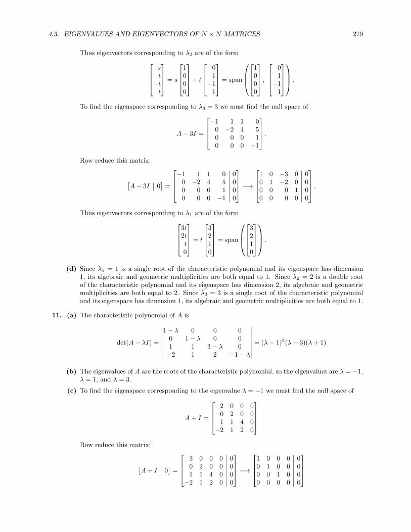
4.3. EIGENVALUES AND EIGENVECTORS OF N ×N MATRICES 279
Thus eigenvectors corresponding to λ2 are of the formst−tt
= s
1000
+ t
01−1
1
= span
1000
,
01−1
1
.
To find the eigenspace corresponding to λ3 = 3 we must find the null space of
A− 3I =
−1 1 1 0
0 −2 4 50 0 0 10 0 0 −1
.Row reduce this matrix:
[A− 3I 0
]=
−1 1 1 0 0
0 −2 4 5 00 0 0 1 00 0 0 −1 0
−→
1 0 −3 0 00 1 −2 0 00 0 0 1 00 0 0 0 0
.Thus eigenvectors corresponding to λ1 are of the form
3t2tt0
= t
3210
= span
3210
.
(d) Since λ1 = 1 is a single root of the characteristic polynomial and its eigenspace has dimension1, its algebraic and geometric multiplicities are both equal to 1. Since λ2 = 2 is a double rootof the characteristic polynomial and its eigenspace has dimension 2, its algebraic and geometricmultiplicities are both equal to 2. Since λ3 = 3 is a single root of the characteristic polynomialand its eigenspace has dimension 1, its algebraic and geometric multiplicities are both equal to 1.
11. (a) The characteristic polynomial of A is
det(A− λI) =
∣∣∣∣∣∣∣∣1− λ 0 0 0
0 1− λ 0 01 1 3− λ 0−2 1 2 −1− λ
∣∣∣∣∣∣∣∣ = (λ− 1)2(λ− 3)(λ+ 1)
(b) The eigenvalues of A are the roots of the characteristic polynomial, so the eigenvalues are λ = −1,λ = 1, and λ = 3.
(c) To find the eigenspace corresponding to the eigenvalue λ = −1 we must find the null space of
A+ I =
2 0 0 00 2 0 01 1 4 0−2 1 2 0
Row reduce this matrix:
[A+ I 0
]=
2 0 0 0 00 2 0 0 01 1 4 0 0−2 1 2 0 0
−→
1 0 0 0 00 1 0 0 00 0 1 0 00 0 0 0 0

280 CHAPTER 4. EIGENVALUES AND EIGENVECTORS
Thus eigenvectors corresponding to λ = −1 are of the form000t
, so that E−1 = span
0001
.
To find the eigenspace corresponding to the eigenvalue λ = 1 we must find the null space of
A− I =
0 0 0 00 0 0 01 1 2 0−2 1 2 −2
Row reduce this matrix:
[A− I 0
]=
0 0 0 0 0
0 0 0 0 0
1 1 2 0 0
−2 1 2 −2 0
−→
1 0 0 23 0
0 1 2 − 23 0
0 0 0 0 0
0 0 0 0 0
Thus eigenvectors corresponding to λ = 1 are of the form
− 23 t
−2s+ 23 t
s
t
= s
0
−2
1
0
+ t
− 2
323
0
1
, so that E1 = span
0
−2
1
0
,−2
2
0
3
.
To find the eigenspace corresponding to the eigenvalue λ = 3 we must find the null space of
A− 3I =
−2 0 0 0
0 −2 0 01 1 0 0−2 1 2 −4
Row reduce this matrix:
[A− 3I 0
]=
−2 0 0 0 0
0 −2 0 0 0
1 1 0 0 0
−2 1 2 −4 0
−→
1 0 0 0 0
0 1 0 0 0
0 0 1 −2 0
0 0 0 0 0
Thus eigenvectors corresponding to λ = 3 are of the form
0
0
2t
t
, so that E3 = span
0
0
2
1
.
(d) Since λ = 3 and λ = −1 are single roots of the characteristic polynomial, they each have algebraicmultiplicity 1; their eigenspaces are each one-dimensional, so those two eigenvalues have geometricmultiplicity 1 as well. Since λ = 1 is a double root of the characteristic polynomial, it has algebraicmultiplicity 2; since its eigenspace is two-dimensional, it also has geometric multiplicity 2.

4.3. EIGENVALUES AND EIGENVECTORS OF N ×N MATRICES 281
12. (a) The characteristic polynomial of A is
det(A− λI) =
∣∣∣∣∣∣∣∣4− λ 0 1 0
0 4− λ 1 10 0 1− λ 20 0 3 −λ
∣∣∣∣∣∣∣∣= −3
∣∣∣∣∣∣4− λ 0 0
0 4− λ 10 0 2
∣∣∣∣∣∣+ (−λ)
∣∣∣∣∣∣4− λ 0 1
0 4− λ 10 0 1− λ
∣∣∣∣∣∣= −6(4− λ)2 − λ(1− λ)(4− λ)2
= (4− λ)2(λ2 − λ− 6) = (4− λ)2(λ− 3)(λ+ 2)
since each of the 3 × 3 matrices is upper triangular, so that by Theorem 4.2 their determinantsare the product of their diagonal elements.
(b) The eigenvalues of A are the roots of the characteristic polynomial, which are λ1 = 4, λ2 = 3,and λ3 = −2.
(c) To find the eigenspace corresponding to λ1 = 4 we must find the null space of
A− 4I =
0 0 1 00 0 1 10 0 −3 20 0 0 −4
.Row reduce this matrix:
[A− 4I 0
]=
0 0 1 0 00 0 1 1 00 0 −3 2 00 0 0 −4 0
−→
0 0 1 0 00 0 0 1 00 0 0 0 00 0 0 0 0
.Thus eigenvectors corresponding to λ1 are of the form
st00
= s
1000
+ t
0100
= span
1000
,
0100
.
To find the eigenspace corresponding to λ2 = 3 we must find the null space of
A− 3I =
1 0 1 00 1 1 10 0 −2 20 0 0 −3
.Row reduce this matrix:
[A− 3I 0
]=
1 0 1 0 00 1 1 1 00 0 −2 2 00 0 0 −3 0
−→
1 0 0 1 00 1 0 2 00 0 1 −1 00 0 0 0 0
.Thus eigenvectors corresponding to λ1 are of the form
−t−2ttt
= t
−1−2
11
= span
−1−2
11
.

282 CHAPTER 4. EIGENVALUES AND EIGENVECTORS
To find the eigenspace corresponding to λ3 = −2 we must find the null space of
A+ 2I =
6 0 1 00 6 1 10 0 3 20 0 3 2
.Row reduce this matrix:
[A+ 2I 0
]=
6 0 1 0 0
0 6 1 1 0
0 0 3 2 0
0 0 3 2 0
−→
1 0 0 − 19 0
0 1 0 118 0
0 0 1 23 0
0 0 0 0 0
.Thus eigenvectors corresponding to λ1 are of the form
19 t
− 118 t
− 23 t
t
=
2s
−s−12s
18s
= s
2
−1
−12
18
= span
2
−1
−12
18
.
(d) Since λ1 = 4 is a double root of the characteristic polynomial and its eigenspace has dimension2, its algebraic and geometric multiplicities are both equal to 2. Since λ2 = 3 is a single rootof the characteristic polynomial and its eigenspace has dimension 1, its algebraic and geometricmultiplicities are both equal to 1. Since λ3 = −2 is a single root of the characteristic polynomialand its eigenspace has dimension 1, its algebraic and geometric multiplicities are both equal to 1.
13. We must show that if A is invertible and Ax = λx, then A−1x = 1λx = λ−1x. First note that since A
is invertible, 0 is not an eigenvalue, so that λ 6= 0 and this statement makes sense. Now,
x = (A−1A)x = A−1(Ax) = A−1(λx) = λ(A−1x).
Dividing through by λ gives A−1x = λ−1x as required.
14. The remark referred to in Section 3.3 tells us that if A is invertible and n > 0 is an integer, thenA−n = (A−1)n = (An)−1. Now, part (a) gives us the result in part (c) when n > 0 is an integer. Whenn = 0, the statement says that λ0 = 1 is an eigenvalue of A0 = I, which is true. So it remains to provethe statement for n < 0. We use induction on n. For n = −1, this is the statement that if Ax = λx,then A−1x = λ−1x, which is Theorem 4.18(b). Now assume the statement holds for n = −k, andprove it for n = −(k + 1). Note that by the remark in Section 3.3,
A−(k+1) = (Ak+1)−1 = (AkA)−1 = A−1(Ak)−1 = A−1A−k.
Now
A−(k+1)x = A−1(A−kx)inductive
hypothesis= A−1(λ−kx) = λ−kA−1x
n=−1= λ−kλ−1x = λ−(k+1)x
and we are done.
15. If we can express x as a linear combination of the eigenvectors, it will be easy to compute A10x since
we know what A10 does to the eigenvectors. To so express x, we solve the system[v1 v2
] [c1c2
]=
[51
],
which is
c1 + c2 = 5
−c1 + c2 = 1.

4.3. EIGENVALUES AND EIGENVECTORS OF N ×N MATRICES 283
This has the solution c1 = 2 and c2 = 3, so that x = 2v1 + 3v2. But by Theorem 4.4(a), v1 and v2
are eigenvectors of A10 with eigenvalues λ101 and λ10
2 . Thus
A10x = A10(2v1 + 3v2) = 2A10v1 + 3A10v2 = 2λ101 v1 + 3λ10
2 v2 =1
512v1 + 3072v2.
Substituting for v1 and v2 gives
A10x =
[3072 + 1
512
3072− 1512
].
16. As in Exercise 15,
Akx = 2 ·(
1
2
)kv1 + 3 · 2kv2 =
[3 · 2k + 21−k
3 · 2k − 21−k
].
As k →∞, the 21−k terms approach zero, so that Akx ≈ 3 · 2kv2.
17. We want to express x as a linear combination of the eigenvectors, say x = c1v1 + c2v2 + c3v3, so wewant a solution of the linear system
c1 + c2 + c3 = 2
c2 + c3 = 1
c3 = 2.
Working from the bottom and substituting gives c3 = 2, c2 = −1, and c1 = 1, so that x = v1−v2+2v3.Then
A20x = A20(v1 − v2 + 2v3)
= A20v1 −A20v2 + 2A20v3
= λ201 v1 − λ20
2 v2 + 2λ203 v3
=
(−1
3
)201
00
− (1
3
)201
10
+ 2 · 120
111
=
22− 1
320
2
.18. As in Exercise 17,
Akx = Ak(v1 − v2 + 2v3)
= Akv1 −Akv2 + 2Akv3
= λk1v1 − λk2v2 + 2λk3v3
=
(−1
3
)k 100
− (1
3
)k 110
+ 2 · 1k1
11
=
± 13k − 1
3k + 2− 1
3k + 22
.
As k →∞, the 13k terms approach zero, and Akx→
222
.

284 CHAPTER 4. EIGENVALUES AND EIGENVECTORS
19. (a) Since (λI)T = λIT = λI, we have
AT − λI = AT − (λI)T = (A− λI)T ,
so that using Theorem 4.10,
det(AT − λI) = det((A− λI)T
)= det(A− λI).
But the left-hand side is the characteristic polynomial of AT , and the right-hand side is thecharacteristic polynomial of A. Thus the two matrices have the same characteristic polynomialand thus the same eigenvalues.
(b) There are many examples. For instance
A =
[1 01 2
]has eigenvalues λ1 = 1 and λ2 = 2, with eigenspaces
E1 = span
([−1
1
]), E2 = span
([01
]).
AT has the same eigenvalues by part (a), but the eigenspaces are
E1 = span
([10
]), E2 = span
([11
]).
20. By Theorem 4.18(b), if λ is an eigenvalue of A, then λm is an eigenvalue of Am = O. But the onlyeigenvalue of O is zero, since Am takes any vector to zero. Thus λm = 0, so that λ = 0.
21. By Theorem 4.18(a), if λ is an eigenvalue of A with eigenvector x, then λ2 is an eigenvalue of A2 = Awith eigenvector x. Since different eigenvalues have linearly independent eigenvectors by Theorem 4.20,we must have λ2 = λ, so that λ = 0 or λ = 1.
22. If Av = λv, then Av− cIv = λv− cIv, so that (A− cI)v = (λ− c)v. But this equation means exactlythat v is an eigenvector of A− cI with eigenvalues λ− c.
23. (a) The characteristic polynomial of A is
∣∣A− λI∣∣ =
∣∣∣∣3− λ 25 −λ
∣∣∣∣ = λ2 − 3λ− 10 = (λ− 5)(λ+ 2).
So the eigenvalues of A are λ1 = 5 and λ2 = −2. For λ1, we have
A− 5I =
[−2 2
5 −5
]→[1 −10 0
],
and for λ2, we have
A+ 2I =
[5 25 2
]→[1 2
50 0
].
It follows that
E5 = span
([11
]), E−2 = span
([− 2
51
])= span
([−2
5
]).
(b) By Theorem 4.4(b), A−1 has eigenvalues 15 and − 1
2 , with
E1/5 = span
([11
]), E−1/2 = span
([−2
5
]).
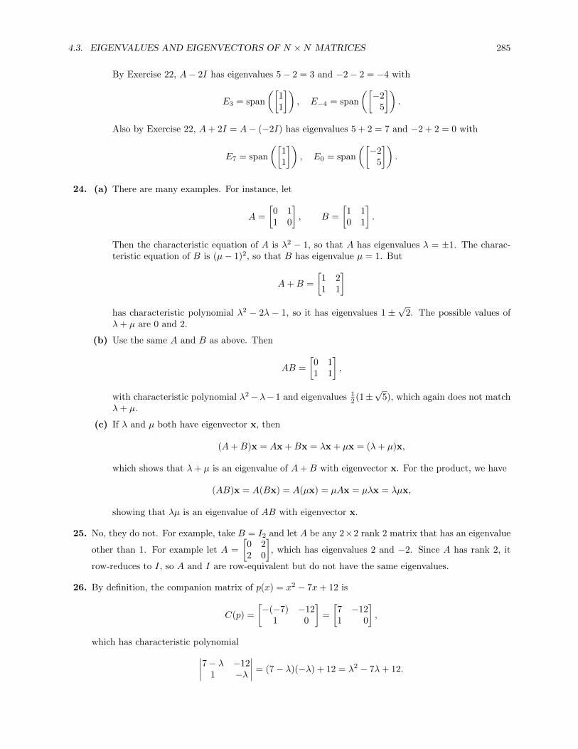
4.3. EIGENVALUES AND EIGENVECTORS OF N ×N MATRICES 285
By Exercise 22, A− 2I has eigenvalues 5− 2 = 3 and −2− 2 = −4 with
E3 = span
([11
]), E−4 = span
([−2
5
]).
Also by Exercise 22, A+ 2I = A− (−2I) has eigenvalues 5 + 2 = 7 and −2 + 2 = 0 with
E7 = span
([11
]), E0 = span
([−2
5
]).
24. (a) There are many examples. For instance, let
A =
[0 11 0
], B =
[1 10 1
].
Then the characteristic equation of A is λ2 − 1, so that A has eigenvalues λ = ±1. The charac-teristic equation of B is (µ− 1)2, so that B has eigenvalue µ = 1. But
A+B =
[1 21 1
]has characteristic polynomial λ2 − 2λ − 1, so it has eigenvalues 1 ±
√2. The possible values of
λ+ µ are 0 and 2.
(b) Use the same A and B as above. Then
AB =
[0 11 1
],
with characteristic polynomial λ2−λ− 1 and eigenvalues 12 (1±
√5), which again does not match
λ+ µ.
(c) If λ and µ both have eigenvector x, then
(A+B)x = Ax +Bx = λx + µx = (λ+ µ)x,
which shows that λ+ µ is an eigenvalue of A+B with eigenvector x. For the product, we have
(AB)x = A(Bx) = A(µx) = µAx = µλx = λµx,
showing that λµ is an eigenvalue of AB with eigenvector x.
25. No, they do not. For example, take B = I2 and let A be any 2×2 rank 2 matrix that has an eigenvalue
other than 1. For example let A =
[0 22 0
], which has eigenvalues 2 and −2. Since A has rank 2, it
row-reduces to I, so A and I are row-equivalent but do not have the same eigenvalues.
26. By definition, the companion matrix of p(x) = x2 − 7x+ 12 is
C(p) =
[−(−7) −12
1 0
]=
[7 −121 0
],
which has characteristic polynomial∣∣∣∣7− λ −121 −λ
∣∣∣∣ = (7− λ)(−λ) + 12 = λ2 − 7λ+ 12.
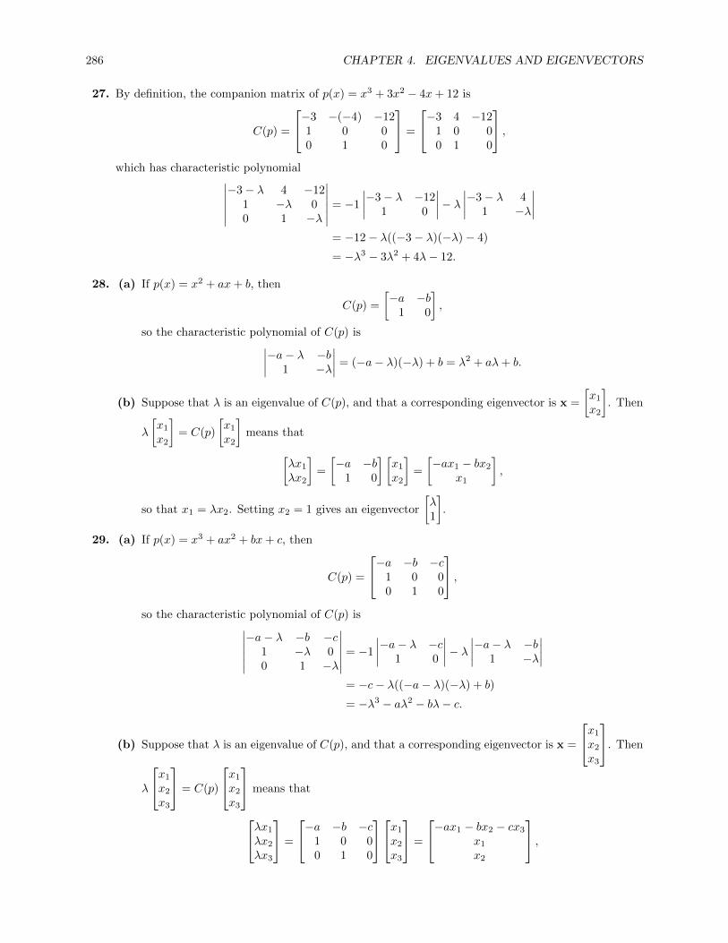
286 CHAPTER 4. EIGENVALUES AND EIGENVECTORS
27. By definition, the companion matrix of p(x) = x3 + 3x2 − 4x+ 12 is
C(p) =
−3 −(−4) −121 0 00 1 0
=
−3 4 −121 0 00 1 0
,which has characteristic polynomial∣∣∣∣∣∣
−3− λ 4 −121 −λ 00 1 −λ
∣∣∣∣∣∣ = −1
∣∣∣∣−3− λ −121 0
∣∣∣∣− λ ∣∣∣∣−3− λ 41 −λ
∣∣∣∣= −12− λ((−3− λ)(−λ)− 4)
= −λ3 − 3λ2 + 4λ− 12.
28. (a) If p(x) = x2 + ax+ b, then
C(p) =
[−a −b
1 0
],
so the characteristic polynomial of C(p) is∣∣∣∣−a− λ −b1 −λ
∣∣∣∣ = (−a− λ)(−λ) + b = λ2 + aλ+ b.
(b) Suppose that λ is an eigenvalue of C(p), and that a corresponding eigenvector is x =
[x1
x2
]. Then
λ
[x1
x2
]= C(p)
[x1
x2
]means that[
λx1
λx2
]=
[−a −b
1 0
] [x1
x2
]=
[−ax1 − bx2
x1
],
so that x1 = λx2. Setting x2 = 1 gives an eigenvector
[λ1
].
29. (a) If p(x) = x3 + ax2 + bx+ c, then
C(p) =
−a −b −c1 0 00 1 0
,so the characteristic polynomial of C(p) is∣∣∣∣∣∣
−a− λ −b −c1 −λ 00 1 −λ
∣∣∣∣∣∣ = −1
∣∣∣∣−a− λ −c1 0
∣∣∣∣− λ ∣∣∣∣−a− λ −b1 −λ
∣∣∣∣= −c− λ((−a− λ)(−λ) + b)
= −λ3 − aλ2 − bλ− c.
(b) Suppose that λ is an eigenvalue of C(p), and that a corresponding eigenvector is x =
x1
x2
x3
. Then
λ
x1
x2
x3
= C(p)
x1
x2
x3
means that
λx1
λx2
λx3
=
−a −b −c1 0 00 1 0
x1
x2
x3
=
−ax1 − bx2 − cx3
x1
x2
,

4.3. EIGENVALUES AND EIGENVECTORS OF N ×N MATRICES 287
so that x1 = λx2 and x2 = λx3. Setting x3 = 1 gives an eigenvector
λ2
λ1
.
30. Using Exercise 28, the characteristic polynomial of the matrix
C(p) =
[−a −b
1 0
]is λ2 + aλ+ b. If we want this matrix to have eigenvalues 2 and 5, then λ2 + aλ+ b = (λ− 2)(λ− 5) =λ2 − 7λ+ 10, so we can take
A =
[7 −101 0
].
31. Using Exercise 28, the characteristic polynomial of the matrix
C(p) =
−a −b −c1 0 00 1 0
is −(λ3 + aλ2 + bλ+ c). If we want this matrix to have eigenvalues −2, 1, and 3, then
−(λ3 + aλ2 + bλ+ c) = −(λ+ 2)(λ− 1)(λ− 3) = λ3 − 2λ2 − 5λ+ 6,
so we can take
A =
2 5 −61 0 00 1 0
.32. (a) Exercises 28 and 29 provide a basis for the induction, proving the cases n = 2 and n = 3. So
assume that the statement holds for n = k; that is, that∣∣∣∣∣∣∣∣∣∣∣
−ak−1 − λ −ak−2 · · · −a1 −a0
1 −λ · · · 0 0
0 1. . . 0 0
0 0 · · · −λ 00 0 · · · 1 −λ
∣∣∣∣∣∣∣∣∣∣∣= (−1)kp(λ),
where p(x) = xk+ak−1xk−1 + · · ·+a1x+a0. Now suppose that q(x) = xk+1 +bkx
k+ · · ·+b1x+b0has degree k + 1; then
C(q) =
∣∣∣∣∣∣∣∣∣∣∣
−bk − λ −bk−1 · · · −b1 −b01 −λ · · · 0 0
0 1. . . 0 0
0 0 · · · −λ 00 0 · · · 1 −λ
∣∣∣∣∣∣∣∣∣∣∣.
Evaluate this determinant by expanding along the last column, giving
C(q) = (−1)k(−b0)
∣∣∣∣∣∣∣∣∣1 −λ · · · 0
0 1. . . 0
0 0 · · · −λ0 0 · · · 1
∣∣∣∣∣∣∣∣∣+ (−λ)
∣∣∣∣∣∣∣∣∣∣∣
−bk − λ −bk−1 · · · −b2 −b11 −λ · · · 0 0
0 1. . . 0 0
0 0 · · · −λ 00 0 · · · 1 −λ
∣∣∣∣∣∣∣∣∣∣∣.
The first determinant is of an upper triangular matrix, so it is the product of its diagonal entries,which is 1. The second determinant is the characteristic polynomial of xk+bkx
k−1 + · · ·+b2x+b1,

288 CHAPTER 4. EIGENVALUES AND EIGENVECTORS
which is a kth degree polynomial. So by the inductive hypothesis, this determinant is (−1)k(λk +bkλ
k−1 + · · ·+ b2λ+ b1). So the entire expression becomes
C(q) = (−1)k(−b0)− λ((−1)k(λk + bkλ
k−1 + · · ·+ b2λ+ b1))
= (−1)k+1b0 + (−1)k+1(λk+1 + bkλk + · · ·+ b2λ
2 + b1λ)
= (−1)k+1(λk+1 + bkλk + · · ·+ b2λ
2 + b1λ+ b0)
= (−1)k+1q(λ).
(b) The method is quite similar to Exercises 28(b) and 29(b). Suppose that λ is an eigenvalue of C(p)with eigenvector
x =
x1
x2
...xn−1
xn
.Then λx = C(p)x, so that
λx1
λx2
...λxn−1
λxn
=
−an−1 −an−2 · · · −a1 −a0
1 0 · · · 0 00 1 · · · 0 0...
.... . .
......
0 0 · · · 1 0
x1
x2
...xn−1
xn
=
−an−1x1 − an−2x2 − · · · − a1xn−1 − a0xn
x1
x2
...xn−1
.
But this means that xi = λxi+1 for i = 1, 2, . . . , n− 1. Setting xn = 1 gives an eigenvector
x =
λn−1
λn−2
...λ1
.
33. The characteristic polynomial of A is
cA(λ) = det(A− λI) =
∣∣∣∣1− λ −12 3− λ
∣∣∣∣ = (1− λ)(3− λ) + 2 = λ2 − 4λ+ 5.
Now,
A2 =
[1 −12 3
]2
=
[−1 −4
8 7
],
so that
cA(A) = A2 − 4A+ 5I2
=
[−1 −4
8 7
]− 4
[1 −12 3
]+ 5
[1 00 1
]= O.

4.3. EIGENVALUES AND EIGENVECTORS OF N ×N MATRICES 289
34. The characteristic polynomial of A is
cA(λ) = det(A− λI) =
∣∣∣∣∣∣1− λ 1 0
1 −λ 10 1 1− λ
∣∣∣∣∣∣ = −λ3 + 2λ2 + λ− 2.
Now,
A2 =
1 1 01 0 10 1 1
2
=
2 1 11 2 11 1 2
, A3 =
1 1 01 0 10 1 1
3
=
3 3 23 2 32 3 3
,so that
cA(A) = −A3 + 2A2 +A− 2I3
= −
3 3 23 2 32 3 3
+ 2
2 1 11 2 11 1 2
+
1 1 01 0 10 1 1
− 2
1 0 00 1 00 0 1
=
−3 + 4 + 1− 2 −3 + 2 + 1− 0 −2 + 2 + 0− 0−3 + 2 + 1− 0 −2 + 4 + 0− 2 −3 + 2 + 1− 0−2 + 2 + 0− 0 −3 + 2 + 1− 0 −3 + 4 + 1− 2
= O.
35. Since A2 − 4A+ 5I = 0, we have A2 = 4A− 5I, and
A3 = A(4A− 5I) = 4A2 − 5A = 4(4A− 5I)− 5A = 11A− 20I
A4 = (A2)(A2) = (4A− 5I)(4A− 5I) = 16A2 − 40A+ 25I = 16(4A− 5I)− 40A+ 25I = 24A− 55I.
36. Since −A3 + 2A2 +A− 2I = 0, we have
A3 = 2A2 +A− 2I,
A4 = A(A3) = A(2A2 +A− 2I) = 2A3 +A2 − 2A = 2(2A2 +A− 2I) +A2 − 2A = 5A2 − 4I.
37. Since A2 − 4A+ 5I = 0, we get A(A− 4I) = −5I. Then solving for A−1 yields
A−1 = −1
5A− −4
5I = −1
5A+
4
5I
A−2 =(A−1
)2=
(−1
5A+
4
5I
)2
=1
25A2 − 8
25A+
16
25I2 =
1
25(4A− 5I)− 8
25A+
16
25I = − 4
25A+
11
25I.
38. Since −A3 + 2A2 +A− 2I = 0, rearranging terms gives A(−A2 + 2A+ I) = 2I. Then solving for A−1
yields (using Exercise 36)
A−1 =1
2I(−A2 + 2A+ I) = −1
2A2 +A+
1
2I
A−2 =(A−1
)2=
(−1
2A2 +A+
1
2I
)2
=1
4A4 −A3 +
1
2A2 +A+
1
4I2
=1
4(5A2 − 4I)− (2A2 +A− 2I) +
1
2A2 +A+
1
4I
= −1
4A2 +
5
4I.

290 CHAPTER 4. EIGENVALUES AND EIGENVECTORS
39. Apply Exercise 69 in Section 4.2 to the matrix A− λI:
cA(λ) = det(A− λI) = det
[P − λI QO S − λI
]= (det(P − λI))(det(S − λI)) = cP (λ)cS(λ).
(Note that neither O or Q is affected by subtracting an identity matrix, since all the 1’s are along thediagonal, in either P or S.)
40. Start with the equation given in the problem statement:
det(A− λI) = (−1)n(λ− λ1)(λ− λ2) · · · (λ− λn).
This is an equation, so in particular it holds for λ = 0, and it becomes
detA = det(A− 0I) = (−1)n(−λ1)(−λ2) · · · (−λn) = (−1)n(−1)nλ1λ2 · · ·λn = λ1λ2 · · ·λn,
proving the first result. For the second result, we will find the coefficients of λn−1 on the left and rightsides. On the left side, the easiest method given the tools we have is induction on n. For n = 2,
det(A− λI) = det
[a11 − λ a12
a21 a22 − λ
]= (a11 − λ)(a22 − λ)− a12a21 = λ2 − (a11 + a22)λ− a12a21,
so that the coefficient of λn−1 = λ is − tr(A). Claim that in general, for n ≥ 1, the coefficient of λn−1
in det(A−λI) is (−1)n−1 tr(A). Suppose this statement holds for n = k. Then if A is (k+ 1)× (k+ 1),we have (expanding along the first column of A− λI)
detA = (a11 − λ) det(A11 − λI) +
k+1∑i=2
(−1)i+1ai1 det(Ai1 − λI).
Now, the terms in the sum on the right each consist of a constant times the determinant of a k × kmatrix derived by removing row i and column 1 from A. Since i > 1, this means we have removedboth the entries a11 − λI and ai1 − λI from A, so that there are only k − 1 entries in A that containλ. So the sum on the right cannot produce any terms with λk. For the other term, note that A11−λIis a k × k matrix; using the inductive hypothesis we see that the coefficient of λk−1 in det(A11 − λI)is (−1)k−1 tr(A11). Now
detA = (a11 − λ)((−1)kλk + (−1)k−1 tr(A11)λk−1 + . . . ) +∑
. . . ,
so that the coefficient of λk in detA is
(−1)ka11− (−1)k−1 tr(A11) = (−1)k(a11 + tr(A11)) = (−1)k(a11 + a22 + · · ·+ ak+1,k+1) = (−1)k tr(A).
Now look at the product on the right in the original expression
det(A− λI) = (−1)n(λ− λ1)(λ− λ2) · · · (λ− λn).
We can get a constant times λn−1 by expanding the right-hand side when exactly n− 1 of the factorsuse λ and one uses λi for some i; that contribution to the λn−1 term in the characteristic polynomialis −λiλn−1. Summing over all possible choices for i shows that the coefficient of the λn−1 term is
(−1)n(−λ1 − λ2 − · · · − λn) = (−1)n+1(λ1 + λ2 + · · ·+ λn) = (−1)n−1(λ1 + λ2 + · · ·+ λn).
Since the coefficient of λn−1 on the left must be the same as that on the right, we have
(−1)n−1 tr(A) = (−1)n−1(λ1 + λ2 + · · ·+ λn), or tr(A) = λ1 + λ2 + · · ·+ λn.
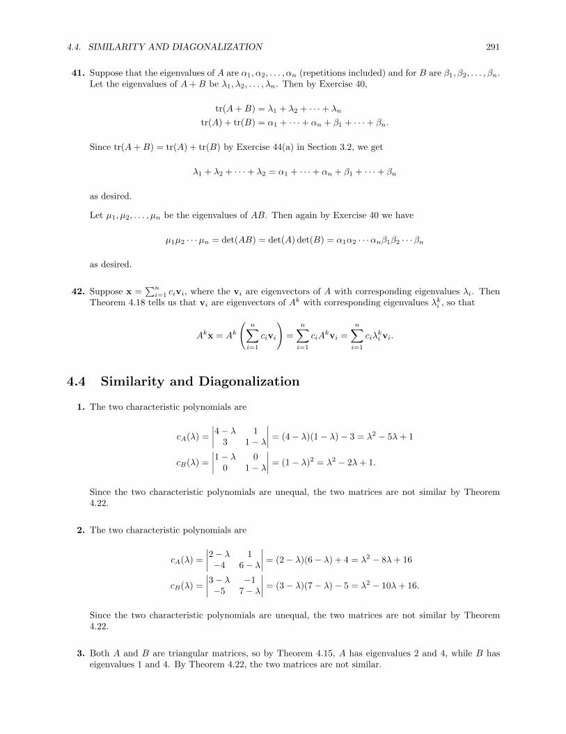
4.4. SIMILARITY AND DIAGONALIZATION 291
41. Suppose that the eigenvalues of A are α1, α2, . . . , αn (repetitions included) and for B are β1, β2, . . . , βn.Let the eigenvalues of A+B be λ1, λ2, . . . , λn. Then by Exercise 40,
tr(A+B) = λ1 + λ2 + · · ·+ λn
tr(A) + tr(B) = α1 + · · ·+ αn + β1 + · · ·+ βn.
Since tr(A+B) = tr(A) + tr(B) by Exercise 44(a) in Section 3.2, we get
λ1 + λ2 + · · ·+ λ2 = α1 + · · ·+ αn + β1 + · · ·+ βn
as desired.
Let µ1, µ2, . . . , µn be the eigenvalues of AB. Then again by Exercise 40 we have
µ1µ2 · · ·µn = det(AB) = det(A) det(B) = α1α2 · · ·αnβ1β2 · · ·βn
as desired.
42. Suppose x =∑ni=1 civi, where the vi are eigenvectors of A with corresponding eigenvalues λi. Then
Theorem 4.18 tells us that vi are eigenvectors of Ak with corresponding eigenvalues λki , so that
Akx = Ak
(n∑i=1
civi
)=
n∑i=1
ciAkvi =
n∑i=1
ciλki vi.
4.4 Similarity and Diagonalization
1. The two characteristic polynomials are
cA(λ) =
∣∣∣∣4− λ 13 1− λ
∣∣∣∣ = (4− λ)(1− λ)− 3 = λ2 − 5λ+ 1
cB(λ) =
∣∣∣∣1− λ 00 1− λ
∣∣∣∣ = (1− λ)2 = λ2 − 2λ+ 1.
Since the two characteristic polynomials are unequal, the two matrices are not similar by Theorem4.22.
2. The two characteristic polynomials are
cA(λ) =
∣∣∣∣2− λ 1−4 6− λ
∣∣∣∣ = (2− λ)(6− λ) + 4 = λ2 − 8λ+ 16
cB(λ) =
∣∣∣∣3− λ −1−5 7− λ
∣∣∣∣ = (3− λ)(7− λ)− 5 = λ2 − 10λ+ 16.
Since the two characteristic polynomials are unequal, the two matrices are not similar by Theorem4.22.
3. Both A and B are triangular matrices, so by Theorem 4.15, A has eigenvalues 2 and 4, while B haseigenvalues 1 and 4. By Theorem 4.22, the two matrices are not similar.

292 CHAPTER 4. EIGENVALUES AND EIGENVECTORS
4. The two characteristic polynomials are
cA(λ) =
∣∣∣∣∣∣1− λ 2 0
0 1− λ −10 −1 1− λ
∣∣∣∣∣∣= (1− λ)
∣∣∣∣1− λ −1−1 1− λ
∣∣∣∣− 2
∣∣∣∣0 −10 1− λ
∣∣∣∣= (1− λ)((1− λ)2 − 1) = (1− λ)(λ2 − 2λ) = −λ3 + 3λ2 − 2λ
cB(λ) =
∣∣∣∣∣∣2− λ 1 1
0 1− λ 02 0 1− λ
∣∣∣∣∣∣= (1− λ)
∣∣∣∣2− λ 12 1− λ
∣∣∣∣= (1− λ)((2− λ)(1− λ)− 2) = (1− λ)(λ2 − 3λ) = −λ3 + 4λ2 − 3λ.
Since the two characteristic polynomials are unequal, the two matrices are not similar by Theorem4.22.
5. By Theorem 4.23, the columns of P are the eigenvectors of A corresponding to the eigenvalues, whichare the diagonal entries of D. Thus
λ1 = 4 with eigenspace span
([11
])λ2 = 3 with eigenspace span
([12
]).
6. By Theorem 4.23, the columns of P are the eigenvectors of A corresponding to the eigenvalues, whichare the diagonal entries of D. Thus
λ1 = 2 with eigenspace span
312
λ2 = 0 with eigenspace span
1−1
0
λ3 = −1 with eigenspace span
01−1
.
7. By Theorem 4.23, the columns of P are the eigenvectors of A corresponding to the eigenvalues, whichare the diagonal entries of D. Thus
λ1 = 6 with eigenspace span
323
λ2 = −2 with eigenspace span
01−1
, 1
0−1
.
8. To determine whether A is diagonalizable, we first compute its eigenvalues:
det(A− λI) =
∣∣∣∣5− λ 22 5− λ
∣∣∣∣ = (5− λ)2 − 4 = λ2 − 10λ+ 21 = (λ− 3)(λ− 7).

4.4. SIMILARITY AND DIAGONALIZATION 293
Since A is a 2× 2 matrix with 2 distinct eigenvalues, it is diagonalizable by Theorem 4.25. To find thediagonalizing matrix P , we find the eigenvectors of A. To find the eigenspace corresponding to λ1 = 3we must find the null space of
A− 3I =
[2 22 2
].
Row reduce this matrix: [A− 3I 0
]=
[2 2 02 2 0
]−→
[1 1 00 0 0
].
Thus eigenvectors corresponding to λ1 are of the form[−tt
]= t
[−1
1
]= span
([−1
1
]).
To find the eigenspace corresponding to λ2 = 7 we must find the null space of
A− 7I =
[−2 2
2 −2
].
Row reduce this matrix: [A− 7I 0
]=
[−2 2 0
2 −2 0
]−→
[1 −1 00 0 0
].
Thus eigenvectors corresponding to λ1 are of the form[tt
]= t
[11
]= span
([11
]).
Thus
P =
[−1 1
1 1
], so that P−1 =
[− 1
212
12
12
]and so by Theorem 4.23,
P−1AP =
[− 1
212
12
12
][5 2
2 5
][−1 1
1 1
]=
[3 0
0 7
].
9. To determine whether A is diagonalizable, we first compute its eigenvalues:
det(A− λI) =
∣∣∣∣−3− λ 4−1 1− λ
∣∣∣∣ = (−3− λ)(1− λ)− 4 · (−1) = λ2 + 2λ+ 1 = (λ+ 1)2.
So the only eigenvalue is λ = −1, with algebraic multiplicity 2. To see if A is diagonalizable, we must seeif its geometric multiplicity is also 2 by finding its eigenvectors. To find the eigenspace correspondingto λ = −1, we must find the null space of
A+ I =
[−2 4−1 2
]by row-reducing it: [
A+ I 0]
=
[−2 4 0−1 2 0
]−→
[1 −2 00 0 0
].
Thus eigenvectors corresponding to λ1 are of the form[2tt
], so a basis for the eigenspace is
[21
].
Thus λ = −1 has geometric multiplicity 1, which is less than the algebraic multiplicity, so that A isnot diagonalizable by Theorem 4.27.

294 CHAPTER 4. EIGENVALUES AND EIGENVECTORS
10. To determine whether A is diagonalizable, we first compute its eigenvalues:
det(A− λI) =
∣∣∣∣∣∣3− λ 1 0
0 3− λ 10 0 3− λ
∣∣∣∣∣∣ = (3− λ)3
since the matrix is a triangular matrix. Thus the only eigenvalue is λ = 3, with algebraic multiplicity3. To see if A is diagonalizable, we must compute the eigenspace corresponding to this eigenvalue. Tofind the eigenspace corresponding to λ = 3 we row-reduce
[A− 3I 0
]:
[A− 3I 0
]=
0 1 0 00 0 1 00 0 0 0
.But this matrix is already row-reduced, and thus the eigenspace iss0
0
= s
100
= span
100
.
Thus the geometric multiplicity is only 1 while the algebraic multiplicity is 3. So by Theorem 4.27,the matrix is not diagonalizable.
11. To determine whether A is diagonalizable, we first compute its eigenvalues:
det(A− λI) =
∣∣∣∣∣∣1− λ 0 1
0 1− λ 11 1 −λ
∣∣∣∣∣∣ = −λ3 + 2λ2 + λ− 2 = −(λ+ 1)(λ− 1)(λ− 2).
Since A is a 3 × 3 matrix with 3 distinct eigenvalues, it is diagonalizable by Theorem 4.25. To findthe diagonalizing matrix P , we find the eigenvectors of A. To find the eigenspace corresponding toλ = −1, we must find the null space of
A+ I =
2 0 10 2 11 1 1
by row-reducing it: [
A+ I 0]
=
2 0 1 0
0 2 1 0
1 1 1 0
−→1 0 1
2 0
0 1 12 0
0 0 0 0
Thus eigenvectors corresponding to λ1 are of the form−
12 t
− 12 t
t
or, clearing fractions
−t−t2t
.
Thus a basis for this eigenspace is
−1−1
2
.
To find the eigenspace corresponding to λ = 1, we must find the null space of
A− I =
0 0 10 0 11 1 −1

4.4. SIMILARITY AND DIAGONALIZATION 295
by row-reducing it: [A− I 0
]=
0 0 1 00 0 1 01 1 −1 0
−→1 1 0 0
0 0 1 00 0 0 0
Thus eigenvectors corresponding to λ1 are of the form−tt
0
, so a basis for the eigenspace is
−110
.To find the eigenspace corresponding to λ = 2, we must find the null space of
A− 2I =
−1 0 10 −1 11 1 −2
by row-reducing it:
[A− 2I 0
]=
−1 0 1 00 −1 1 01 1 −2 0
−→1 0 −1 0
0 1 −1 00 0 0 0
Thus eigenvectors corresponding to λ1 are of the formtt
t
, so a basis for the eigenspace is
111
.Then a diagonalizing matrix P is the matrix whose columns are the eigenvectors of A:
P =
−1 −1 1
−1 1 1
2 0 1
, so that P−1 =
−16 − 1
613
− 12
12 0
13
13
13
and so by Theorem 4.23,
P−1AP =
−16 − 1
613
− 12
12 0
13
13
13
1 0 1
0 1 1
1 1 0
−1 −1 1
−1 1 1
2 0 1
=
−1 0 0
0 1 0
0 0 2
.12. To determine whether A is diagonalizable, we first compute its eigenvalues:
det(A− λI) =
∣∣∣∣∣∣1− λ 0 0
2 2− λ 13 0 1− λ
∣∣∣∣∣∣ = (1− λ)
∣∣∣∣2− λ 10 1− λ
∣∣∣∣ = (1− λ)2(2− λ).
So the eigenvalues are λ1 = 1 with algebraic multiplicity 2, and λ2 = 2 with algebraic multiplicity 1.To find the eigenspace corresponding to λ1 = 1 we row-reduce
[A− I 0
]:
[A− I 0
]=
1 0 0 02 2 1 03 0 1 0
→1 0 0 0
0 1 1 00 0 0 0
.Thus the eigenspace is 0
−tt
= t
0−1
1
= span
0−1
1
.
Thus the geometric multiplicity of this eigenvalue is only 1 while the algebraic multiplicity is 2. So byTheorem 4.27, the matrix is not diagonalizable.

296 CHAPTER 4. EIGENVALUES AND EIGENVECTORS
13. To determine whether A is diagonalizable, we first compute its eigenvalues:
det(A− λI) =
∣∣∣∣∣∣1− λ 2 1−1 −λ 11 1 −λ
∣∣∣∣∣∣ = λ2 − λ3 = −λ2(λ− 1).
So A has eigenvalues 0 and 1. Considering λ = 0, we row-reduce A− 0I = A: 1 2 1 0−1 0 1 0
1 1 0 0
→1 0 −1 0
0 1 1 00 0 0 0
,so that the eigenspace is
span
1−1
1
.
Since λ = 0 has algebraic multiplicity 2 but geometric multiplicity 1, the matrix is not diagonalizable.
14. To determine whether A is diagonalizable, we first compute its eigenvalues:
det(A− λI) =
∣∣∣∣∣∣∣∣2− λ 0 0 2
0 3− λ 2 10 0 3− λ 00 0 0 1− λ
∣∣∣∣∣∣∣∣ = (1− λ)(2− λ)(3− λ)2
since the matrix is upper triangular. So the eigenvalues are λ1 = 1 with algebraic multiplicity 1,λ2 = 2 with algebraic multiplicity 1, and λ3 = 3 with algebraic multiplicity 2. To find the eigenspacecorresponding to λ3 = 3 we row-reduce
[A− 3I 0
]:
[A− 3I 0
]=
−1 0 0 2 0
0 0 2 1 00 0 0 0 00 0 0 −2 0
→
1 0 0 0 00 0 1 0 00 0 0 1 00 0 0 0 0
.Thus the eigenspace is
0t00
= t
0100
= span
0100
.
Thus the geometric multiplicity of this eigenvalue is only 1 while the algebraic multiplicity is 2. So byTheorem 4.27, the matrix is not diagonalizable.
15. Since A is triangular, we can read off its eigenvalues, which are λ1 = 2 and λ2 = −2, each of whichhas algebraic multiplicity 2. Computing eigenspaces, we have
[A− 2I 0
]=
0 0 0 4 00 0 0 0 00 0 −4 0 00 0 0 −4 0
→
0 0 1 0 00 0 0 1 00 0 0 0 00 0 0 0 0
, so E2 has basis
1000
,
0100
[A+ 2I 0
] 4 0 0 4 00 4 0 0 00 0 0 0 00 0 0 0 0
→
1 0 0 1 00 1 0 0 00 0 0 0 00 0 0 0 0
, so E−2 has basis
−1
001
,
0010
.
Since each eigenvalue also has geometric multiplicity 2, the matrix is diagonalizable, and
P =
1 0 −1 00 1 0 00 0 0 10 0 1 0
, D =
2 0 0 00 2 0 00 0 −2 00 0 0 −2

4.4. SIMILARITY AND DIAGONALIZATION 297
provides a solution to
P−1AP =
1 0 0 10 1 0 00 0 0 10 0 1 0
2 0 0 40 2 0 00 0 −2 00 0 0 −2
1 0 −1 00 1 0 00 0 0 10 0 1 0
=
2 0 0 00 2 0 00 0 −2 00 0 0 −2
= D.
16. As in Example 4.29, we must find a matrix P such that
P−1AP = P−1
[−4 6−3 5
]P
is diagonal. To do this, we find the eigenvalues and a basis for the eigenspaces of A. The eigenvaluesof A are the roots of its characteristic polynomial
det(A− λI) =
∣∣∣∣−4− λ 6−3 5− λ
∣∣∣∣ = (−4− λ)(5− λ) + 18 = λ2 − λ− 2.
This polynomial factors as (λ− 2)(λ+ 1), so the eigenvalues are λ1 = −1 and λ2 = 2. The eigenspaceassociated with λ1 can be found by finding the null space of A+ I:
[A+ I 0
]=
[−3 6 0−3 6 0
]→[1 −2 00 0 0
]
Thus a basis for this eigenspace is given by
[21
].
The eigenspace associated with λ2 can be found by finding the null space of A− 2I:
[A− 2I 0
]=
[−6 6 0−3 3 0
]→[1 −1 00 0 0
].
Thus a basis for this eigenspace is given by
[11
].
Set
P =
[1 21 1
], so that P−1 =
[−1 2
1 −1
]Then
D = P−1AP =
[2 00 −1
], so that A5 = PD5P−1 =
[1 21 1
] [32 00 −1
] [−1 2
1 −1
]=
[−34 66−33 65
]17. As in Example 4.29, we must first diagonalize A. To do this, we find the eigenvalues and a basis for
the eigenspaces of A. The eigenvalues of A are the roots of its characteristic polynomial
det(A− λI) =
∣∣∣∣−1− λ 61 −λ
∣∣∣∣ = (−1− λ)(−λ)− 6 = λ2 + λ− 6 = (λ+ 3)(λ− 2),
so the eigenvalues are λ1 = −3 and λ2 = 2. To compute the eigenspaces, we row-reduce[A+ 3I 0
]and
[A− 2I 0
]:
[A+ 3I 0
]=
[2 6 01 3 0
]→[1 3 00 0 0
], so E−3 has basis
{[−3
1
]}[A− 2I 0
]=
[−3 6 0
1 −2 0
]→[1 −2 00 0 0
]so E2 has basis
{[21
]}.

298 CHAPTER 4. EIGENVALUES AND EIGENVECTORS
Thus
P =
[−3 2
1 1
]P−1 =
[15 − 2
515
35
]D =
[−3 0
0 2
]satisfy P−1AP = D, so that[
−1 6
1 0
]10
= (PDP−1)10 = PD10P=1
=
[−3 2
1 1
][−3 0
0 2
]10 [15 − 2
515
35
]
=
[−3 2
1 1
][(−3)10 0
0 210
]10 [15 − 2
515
35
]
=
[35,839 −69,630
−11,605 24,234
].
18. As in Example 4.29, we must first diagonalize A. To do this, we find the eigenvalues and a basis forthe eigenspaces of A. The eigenvalues of A are the roots of its characteristic polynomial
det(A− λI) =
∣∣∣∣4− λ −3−1 2− λ
∣∣∣∣ = (4− λ)(2− λ)− 3 = λ2 − 6λ+ 5 = (λ− 5)(λ− 1),
so the eigenvalues are λ1 = 1 and λ2 = 5. To compute the eigenspaces, we row-reduce[A− I 0
]and[
A− 5I 0]:
[A− I 0
]=
[3 −3 0−1 1 0
]→[1 −1 00 0 0
], so that E1 has basis
{[11
]},
[A− 5I 0
]=
[−1 −3 0−1 −3 0
]→[1 3 00 0 0
], so that E5 has basis
{[−3
1
]}.
Set
P =
[1 −3
1 1
], so that P−1 =
[14
34
− 14
14 ,
], D =
[1 0
0 5
].
Then
A−6 = PD−6P−1 =
[1 −3
1 1
][1 0
0 5−6
][14
34
− 14
14
]=
[390756
1171856
390656
1171956
].
19. As in Example 4.29, we must first diagonalize A. To do this, we find the eigenvalues and a basis forthe eigenspaces of A. The eigenvalues of A are the roots of its characteristic polynomial
det(A− λI) =
∣∣∣∣−λ 31 2− λ
∣∣∣∣ = (−λ)(2− λ)− 3 = λ2 − 2λ− 3 = (λ− 3)(λ+ 1),
so the eigenvalues are λ1 = 3 and λ2 = −1. To compute the eigenspaces, we row-reduce[A− 3I 0
]and
[A+ I 0
]:
[A− 3I 0
]=
[−3 3 0
1 −1 0
]→[1 −1 00 0 0
], so that E3 has basis
{[11
]},
[A+ I 0
]=
[1 3 01 3 0
]→[1 3 00 0 0
], so that E−1 has basis
{[−3
1
]}.

4.4. SIMILARITY AND DIAGONALIZATION 299
Set
P =
[1 −3
1 1
], so that P−1 =
[14
34
− 14
14 ,
], D =
[3 0
0 −1
].
Then
Ak = PDkP−1 =
[1 −3
1 1
][3k 0
0 (−1)k
][14
34
− 14
14
]
=
[3k+3(−1)k
43k+1−3(−1)k
43k−(−1)k
43k+1+(−1)k
4
].
20. As in Example 4.29, we must first diagonalize A. To do this, we find the eigenvalues and a basis forthe eigenspaces of A. The eigenvalues of A are the roots of its characteristic polynomial
det(A− λI) =
∣∣∣∣∣∣2− λ 1 2
2 1− λ 22 1 2− λ
∣∣∣∣∣∣ = 5λ2 − λ3 = −λ2(λ− 5),
so the eigenvalues are λ1 = 0 and λ2 = 5. To compute the eigenspaces we row-reduce[A− 0I 0
]and[
A− 5I 0]:
[A 0
]=
2 1 2 0
2 1 2 0
2 1 2 0
→
1 12 1 0
0 0 0 0
0 0 0 0
, so E0 has basis
−1
2
0
,−1
0
1
[A− 5I 0
]=
−3 1 2 02 −4 2 02 1 −3 0
→1 0 −1 0
0 1 −1 00 0 0 0
, so E5 has basis
1
11
.
Set
P =
−1 −1 1
2 0 1
0 1 1
, so that P−1 =
− 1
525 − 1
5
− 25 − 1
535
25
15
25
.Then
D = P−1AP =
0 0 00 0 00 0 5
,so that
A8 = PD8P−1 =
−1 −1 1
2 0 1
0 1 1
0 0 0
0 0 0
0 0 58
− 1
525 − 1
5
− 25 − 1
535
25
15
25
=
156250 78125 156250
156250 78125 156250
156250 78125 156250
.21. As in Example 4.29, we must first diagonalize A. To do this, we find the eigenvalues and a basis for
the eigenspaces of A. Since A is upper triangular, its eigenvalues are the diagonal entries, which areλ1 = −1 and λ2 = 1. To compute the eigenspaces, we row-reduce
[A+ I 0
]and
[A− I 0
]:
[A+ I 0
]=
2 1 1 0
0 0 0 0
0 0 0 0
→1 1
212 0
0 0 0 0
0 0 0 0
, so E−1 has basis
−1
2
0
,−1
0
2
,
[A− I 0
]=
0 1 1 00 −2 0 00 0 −2 0
→0 1 0 0
0 0 1 00 0 0 0
, so E1 has basis
1
00
.

300 CHAPTER 4. EIGENVALUES AND EIGENVECTORS
Set
P =
−1 −1 1
0 2 0
2 0 0
, so that P−1 =
0 0 1
2
0 12 0
1 12
12
.Then
D = P−1AP =
−1 0 00 −1 00 0 1
,so that
A2015 = PD2015P−1 =
−1 −1 1
0 2 0
2 0 0
(−1)2015 0 0
0 (−1)2015 0
0 0 12015
0 0 12
0 12 0
1 12
12
=
−1 −1 1
0 2 0
2 0 0
−1 0 0
0 −1 0
0 0 1
0 0 12
0 12 0
1 12
12
=
1 1 1
0 −1 0
0 0 −1
= A.
22. As in Example 4.29, we must first diagonalize A. To do this, we find the eigenvalues and a basis forthe eigenspaces of A. The eigenvalues of A are the roots of its characteristic polynomial
det(A− λI) =
∣∣∣∣∣∣2− λ 0 1
1 1− λ 11 0 2− λ
∣∣∣∣∣∣= (1− λ)
∣∣∣∣2− λ 11 2− λ
∣∣∣∣= (1− λ)((2− λ)2 − 1) = (1− λ)(λ2 − 4λ+ 3) = −(λ− 1)2(λ− 3).
Thus the eigenvalues are λ1 = 1 and λ2 = 3. To compute the eigenspaces, we row-reduce[A− I 0
]and
[A− 3I 0
].
[A− I 0
]=
1 0 1 01 0 1 01 0 1 0
→1 0 1 0
0 0 0 00 0 0 0
, so E1 has basis
−1
01
,0
10
[A− 3I 0
]=
−1 0 1 01 −2 1 01 0 −1 0
→1 0 −1 0
0 1 −1 00 0 0 0
, so E3 has basis
1
11
.
Set
P =
1 −1 0
1 0 1
1 1 0
, so that P−1 =
12 0 1
2
− 12 0 1
2
− 12 1 − 1
2
, D =
3 0 0
0 1 0
0 0 1
,

4.4. SIMILARITY AND DIAGONALIZATION 301
so that
Ak = PDkP−1 =
1 −1 0
1 0 1
1 1 0
3k 0 0
0 1k 0
0 0 1k
12 0 1
2
− 12 0 1
2
− 12 1 − 1
2
=
1 −1 0
1 0 1
1 1 0
3k 0 0
0 1 0
0 0 1
12 0 1
2
− 12 0 1
2
− 12 1 − 1
2
=
12 (3k + 1) 0 1
2 (3k − 1)12 (3k − 1) 1 1
2 (3k − 1)12 (3k − 1) 0 1
2 (3k + 1)
23. As in Example 4.29, we must first diagonalize A. To do this, we find the eigenvalues and a basis for
the eigenspaces of A. The eigenvalues of A are the roots of its characteristic polynomial
det(A− λI) =
∣∣∣∣∣∣1− λ 1 1
2 −2− λ 20 1 1− λ
∣∣∣∣∣∣ = −(λ− 1)(λ− 2)(λ+ 3).
Thus the eigenvalues are λ1 = 1, λ2 = 2, and λ2 = −3. To compute the eigenspaces, we row-reduce[A− I 0
],[A− 2I 0
], and
[A+ 3I 0
].
[A− I 0
]=
0 1 0 02 −3 2 00 1 0 0
→1 0 1 0
0 1 0 00 0 0 0
, so E1 has basis
−1
01
[A− 2I 0
]=
−1 1 0 02 −4 2 00 1 −1 0
→1 0 −1 0
0 1 −1 00 0 0 0
, so E2 has basis
1
11
[A+ 3I 0
]=
4 1 0 02 1 2 00 1 4 0
→1 0 −1 0
0 1 4 00 0 0 0
, so E3 has basis
1−4
1
.
Set
P =
−1 1 1
0 1 −4
1 1 1
, so that P−1 =
−12 0 1
225
15
25
110 − 1
5110
, D =
1 0 0
0 2 0
0 0 −3
,so that
Ak = PDkP−1 =
−1 1 1
0 1 −4
1 1 1
1 0 0
0 2k 0
0 0 (−3)k
−
12 0 1
225
15
25
110 − 1
5110
=
110 (5 + (−3)k + 2k+2) 1
5 (2k − (−3)k) 110 (−5 + (−3)k + 2k+2)
− 25 ((−3)k − 2k) 1
5 (4(−3)k + 2k) − 25 ((−3)k − 2k)
110 (−5 + (−3)k + 2k+2) 1
5 (2k − (−3)k) 110 (5 + (−3)k + 2k+2)
.
24. The characteristic polynomial of A is
det(A− λI) =
∣∣∣∣1− λ 10 k − λ
∣∣∣∣ = (λ− 1)(λ− k),

302 CHAPTER 4. EIGENVALUES AND EIGENVECTORS
so that if k 6= 1, then A is a 2×2 matrix with two distinct eigenvalues, so it is diagonalizable. If k = 1,then
A− I =
[0 10 0
],
which gives a one-dimensional eigenspace with basis
[10
]. Since λ = 1 has algebraic multiplicity 2 but
geometric multiplicity 1, A is not diagonalizable. So A is diagonalizable exactly when k 6= 1.
25. The characteristic polynomial of A is
det(A− λI) =
∣∣∣∣1− λ k0 1− λ
∣∣∣∣ = (λ− 1)2.
The only eigenvalue is 1, and then
A− I =
[0 k0 0
].
If k = 0, then A is diagonal to start with, while if k 6= 0, then we get a one-dimensional eigenspace
with basis
[10
]. Since λ = 1 then has algebraic multiplicity 2 but geometric multiplicity 1, A is not
diagonalizable. So A is diagonalizable exactly when k = 0.
26. The characteristic polynomial of A is
det(A− λI) =
∣∣∣∣k − λ 11 −λ
∣∣∣∣ = λ(λ− k)− 1 = λ2 − kλ− 1,
so that A has the eigenvalues λ = k±√k2+42 . Since k2 + 4 is never zero, and always positive, the
eigenvalues of A are real and distinct, so A is diagonalizable for all k.
27. Since A is triangular, the only eigenvalue is 1, with algebraic multiplicity 3. Then
A− I =
0 0 k0 0 00 0 0
.If k = 0, then A is diagonal to start with, while if k 6= 0, then we get a one-dimensional eigenspace
with basis
1
00
,0
10
. Since λ = 1 then has algebraic multiplicity 3 but geometric multiplicity 2,
A is not diagonalizable. So A is diagonalizable exactly when k = 0.
28. Since A is triangular, the eigenvalues are 1, with algebraic multiplicity 2, and 2, with algebraic multi-plicity 1. Then
A− I =
0 k 00 1 00 0 0
→0 1 0
0 0 00 0 0
regardless of the value of k, so λ = 1 has a two-dimensional eigenspace with basis
1
00
,0
01
, i.e.,
with geometric multiplicity 2. Since this is equal to the algebraic multiplicity of λ, we see that A isdiagonalizable for all k.
29. The characteristic polynomial of A is
det(A− λI) =
∣∣∣∣∣∣1− λ 1 k
1 1− λ k1 1 k − λ
∣∣∣∣∣∣ = −λ3 + 2λ2 + kλ2 = −λ2(λ− (k + 2)).

4.4. SIMILARITY AND DIAGONALIZATION 303
If k = −2, then A has only the eigenvalue 0, with algebraic multiplicity 3, and then
A =
1 1 −21 1 −21 1 −2
→1 1 −2
0 0 00 0 0
,so the eigenspace is two-dimensional and therefore the geometric multiplicity is not equal to the alge-braic multiplicity, so that A is not diagonalizable. If k 6= −2, then 0 has algebraic multiplicity 2, andthen
A =
1 1 −k1 1 −k1 1 −k
→1 1 −k
0 0 00 0 0
,and the eigenspace is again two-dimensional, so the geometric multiplicity equals the algebraic multi-plicity and A is diagonalizable. Thus A is diagonalizable exactly when k 6= −2.
30. We are given that A ∼ B, so that B = P−1AP for some invertible matrix P , and that B ∼ C, so thatC = Q−1BQ for some invertible matrix Q. But then
C = Q−1BQ = Q−1P−1APQ = (PQ)−1APQ,
so that C is R−1AR for the invertible matrix R = PQ.
31. A is invertible if and only if detA 6= 0. But since A and B are similar, detA = detB by part (a) ofthis theorem. Thus A is invertible if and only if detB 6= 0, which happens if and only if B is invertible.
32. By Exercise 61 in Section 3.5, if U is invertible then rankA = rank(UA) = rank(AU). Now, since Aand B are similar, we have B = P−1AP for some invertible matrix P , so that
rankB = rank(P−1(AP )) = rank(AP ) = rankA,
using the result above twice.
33. Suppose that B = P−1AP where P is invertible. This can be rewritten as BP−1 = P−1A. Let λ bean eigenvalue of A with eigenvector x. Then
B(P−1x) = (BP−1)x = (P−1A)x = P−1(Ax) = P−1(λx) = λ(P−1x).
Thus P−1x is an eigenvector for B, corresponding to λ. So every eigenvalue of A is also an eigenvalueof B. By writing the similarity equation as A = Q−1BQ, we see in exactly the same way that everyeigenvalue of B is an eigenvalue of A. So A and B have the same eigenvalues. (Note that we have alsoproven a relationship between the eigenvectors corresponding to a given eigenvalue).
34. Suppose that A ∼ B, say A = P−1BP . Then if m = 0, we have Am = Bm = I, so that A0 ∼ B0. Ifm > 0, then
Am =(P−1BP
)m= P−1BP · P−1BP · · ·P−1BP · P−1BP︸ ︷︷ ︸
m times
= P−1BmP.
But Am = P−1BmP means that Am ∼ Bm.
35. From part (f), Am ∼ Bm for m ≥ 0. If m < 0, then
Am =(A−m
)−1=(P−1B−mP
)−1
since A−m and B−m are similar because −m > 0. But(P−1B−mP
)−1= P−1 (B−m)
−1 (P−1
)−1=
P−1BmP . Thus Am ∼ Bm for m < 0, so they are similar for all integers m.
36. Let P = B−1. ThenBA = BABB−1 = B(AB)B−1 = P−1(AB)P,
showing that AB ∼ BA.

304 CHAPTER 4. EIGENVALUES AND EIGENVECTORS
37. Exercise 45 in Section 3.2 shows that if A and B are n × n, then tr(AB) = tr(BA). But then ifB = P−1AP , we have
trB = tr(P−1AP ) = tr((P−1A)P ) = tr(P (P−1A)) = tr((PP−1)A) = trA.
38. A is triangular, so it has eigenvalues −1 and 3. For B, we have
det(B − λI) =
∣∣∣∣1− λ 22 1− λ
∣∣∣∣ = (1− λ)2 − 4 = λ2 − 2λ− 3 = (λ+ 1)(λ− 3).
So the eigenvalues of B are also −1 and 3, and thus
A ∼ B ∼[−1 0
0 3
]= D.
Reducing A+ I and A− 3I shows that E−1 = span
([1−4
])and E3 = span
([10
]). Reducing B + I
and B − 3I shows that E−1 = span
([1−1
])and E3 = span
([11
]). Thus
D = Q−1AQ =
[0 1
4
1 − 14
][3 1
0 −1
][1 1
−4 0
]
D = R−1BR =
[12 − 1
212
12
][1 2
2 1
][1 1
−1 1
],
so that finallyB = RDR−1 = RQ−1AQR−1 = (QR−1)−1A(QR−1).
Thus
P = QR−1 =
[1 0−2 2
]is an invertible matrix such that B = P−1AP .
39. We have
det(A− λI) =
∣∣∣∣5− λ −34 −2− λ
∣∣∣∣ = (5− λ)(−2− λ) + 12 = λ2 − 3λ+ 2 = (λ− 1)(λ− 2)
det(B − λI) =
∣∣∣∣−1− λ 1−6 4− λ
∣∣∣∣ = (−1− λ)(4− λ) + 6 = λ2 − 3λ+ 2 = (λ− 1)(λ− 2).
So A and B both have eigenvalues 1 and 2, so that
A ∼ B ∼[1 00 2
]= D.
Reducing A− I and A− 2I shows that E1 = span
([34
])and E2 = span
([11
]). Reducing B − I and
B − 2I shows that E1 = span
([12
])and E3 = span
([13
]). Thus
D = Q−1AQ =
[−1 1
4 −3
] [5 −34 −2
] [3 14 1
]D = R−1BR =
[3 −1−2 1
] [−1 1−6 4
] [1 12 3
],

4.4. SIMILARITY AND DIAGONALIZATION 305
so that finallyB = RDR−1 = RQ−1AQR−1 = (QR−1)−1A(QR−1).
Thus
P = QR−1 =
[7 −2
10 −3
]is an invertible matrix such that B = P−1AP .
40. A is upper triangular, so it has eigenvalues −2, 1, and 2. For B, we have
det(B − λI) =
∣∣∣∣∣∣3− λ 2 −5
1 2− λ −12 2 −4− λ
∣∣∣∣∣∣ = −(λ+ 2)(λ− 1)(λ− 2),
So B also has eigenvalues −2, 1, and 2, so that
A ∼ B ∼
−2 0 00 1 00 0 2
= D.
Reducing A+ 2I, A− I, and A− 2I gives
E−2 = span
1−4
0
, E1 = span
1−1−3
, E2 = span
100
.
Reducing B + 2I, B − I, and B − 2I gives
E−2 = span
101
, E1 = span
1−1
0
, E2 = span
121
.
Therefore
D = Q−1AQ =
0 − 14
112
0 0 − 13
1 14
14
2 1 0
0 −2 1
0 0 1
1 1 1
−4 −1 0
0 −3 0
D = R−1BR =
−12 − 1
232
1 0 −112
12 − 1
2
3 2 −5
1 2 −1
2 2 −4
1 1 1
0 −1 2
1 0 1
,so that finally
B = RDR−1 = RQ−1AQR−1 = (QR−1)−1A(QR−1).
Thus
P = QR−1 =
1 0 01 2 −5−3 0 3
is an invertible matrix such that B = P−1AP .
41. We have
det(A− λI) =
∣∣∣∣∣∣1− λ 0 2
1 −1− λ 12 0 1− λ
∣∣∣∣∣∣ = −(λ+ 1)2(λ− 3)
det(B − λI) =
∣∣∣∣∣∣−3− λ −2 0
6 5− λ 04 4 −1− λ
∣∣∣∣∣∣ = −(λ+ 1)2(λ− 3),

306 CHAPTER 4. EIGENVALUES AND EIGENVECTORS
so that A and B both have eigenvalues −1 (of algebraic multiplicity 2) and 3. Therefore
A ∼ B ∼
−1 0 00 −1 00 0 3
= D.
Reducing A+ I and A− 3I gives
E−1 = span
10−1
,0
10
, E3 = span
212
.
Reducing B + I and B − 3I gives
E−1 = span
1−1
0
,0
01
, E3 = span
1−3−2
.
Therefore
D = Q−1AQ =
12 0 − 1
2
− 14 1 − 1
414 0 1
4
1 0 2
1 −1 1
2 0 1
1 0 2
0 1 1
−1 0 2
D = R−1BR =
32
12 0
−1 −1 1
− 12 − 1
2 0
−3 −2 0
6 5 0
4 4 −1
1 0 1
−1 0 −3
0 1 −2
,so that finally
B = RDR−1 = RQ−1AQR−1 = (QR−1)−1A(QR−1).
Thus
P = QR−1 =
12 − 1
2 0
− 32 − 3
2 1
− 52 − 3
2 0
is an invertible matrix such that B = P−1AP .
42. Suppose that B = P−1AP . This gives PB = AP , so that (PB)T = (AP )T . Expanding yieldsBTPT = PTAT , so that BT ∼ AT and thus AT ∼ BT .
43. Suppose that P−1AP = D, where D is diagonal. Then
D = DT = (P−1AP )T = PTAT (PT )−1.
Now let Q = (PT )−1; the equation above becomes D = Q−1ATQ, so that AT is diagonalizable.
44. If A is invertible, it has no zero eigenvalues. So if it is diagonalizable, the diagonal matrix D is alsoinvertible since none of the diagonal entries are zero. Then D−1 is also diagonal, consisting of theinverses of each of the diagonal entries of D. Suppose that D = P−1AP . Then
D−1 =(P−1AP
)−1= P−1A−1
(P−1
)−1= P−1A−1P,
showing that A−1 is also diagonalizable (and, incidentally, showing again that the eigenvalues of A−1
are the inverses of the eigenvalues of A, by looking at the entries of D−1.)
45. Suppose that A is diagonalizable, and that λ is its only eigenvalue. Then if D = P−1AP is diagonal,all of its diagonal entries must equal λ, so that D = λI. Then λI = P−1AP implies that P (λI)P−1 =PP−1APP−1 = A. However, P (λI)P−1 = λPIP−1 = λI. Thus A = λI.

4.4. SIMILARITY AND DIAGONALIZATION 307
46. Since A and B each have n distinct eigenvalues, they are both diagonalizable by Theorem 4.25. Recallthat diagonal matrices commute: if D and E are both diagonal, then DE = ED. Now, if A and B havethe same eigenvectors, then since the diagonalizing matrix P has columns equal to the eigenvectors,we see that for the same invertible matrix P , both DA = P−1AP and DB = P−1BP are diagonal.But then
AB = (PDAP−1)(PDBP
−1) = PDADBP−1 = PDBDAP
−1 = (PDBP−1)(PDAP
−1) = BA.
Conversely, if AB = BA, let α1, α2, . . . , αn be the distinct eigenvalues of A, and pi the correspondingeigenvectors, which are also distinct since they are linearly independent. Then
A(Bpi) = (AB)pi = (BA)pi = B(Api) = B(αiPi) = αiBpi.
Thus Bpi is also an eigenvector of A corresponding to αi, so it must be a multiple of pi. That is,Bpi = βipi for all i, so that the eigenvectors of B are also pi. So every eigenvector of A is aneigenvector of B. Since B also has n distinct eigenvectors, the set of eigenvectors must be the same.
47. If A ∼ B, then A and B have the same characteristic polynomial, so the algebraic multiplicities oftheir eigenvalues are the same.
48. From the solution to Exercise 33, we know that if B = P−1AP and x is an eigenvector of A witheigenvalue λ, then P−1x is an eigenvalue of B with eigenvalue λ. Therefore, if λ is an eigenvalue of Awith multiplicity m, its eigenspace has a basis consisting of m distinct vectors v1,v2, . . . ,vm, so thatthe vectors P−1v1, P
−1v2, . . . , P−1vm are in the eigenspace of B corresponding to λ. These vectors
are linearly independent since P−1 is an invertible linear transformation. So each of the n eigenvectorsof A corresponds to a distinct eigenvector of B; since each matrix has n eigenvectors, the reverse is trueas well. Therefore the m eigenvalues of B found above are all of the eigenvalues of B corresponding toλ, so that the dimension of the eigenspace of λ for B is m as well. So the geometric multiplicities ofthe eigenvalues of A and B are the same.
49. If D = P−1AP and D is diagonal, then every entry of D is either 0 or 1, since every eigenvalue of Ais either 0 or 1 by assumption. Since D2 is computed by squaring each diagonal entry, we see thatD2 = D. But then PDP−1 = A, and
A2 = (PDP−1)2 = (PDP−1)(PDP−1) = P−1D2P = P−1DP = A,
so that A is idempotent.
50. Suppose that A is nilpotent and diagonalizable, so that D = P−1AP (so that A = PDP−1) andAm = O for some m > 1. Then
Dm = (P−1AP )m = P−1AmP = P−1OP = O.
Since D is diagonal, Dm is found by taking the mth power of each diagonal entry. If this is the zeromatrix, then all the diagonal entries must be zero, so that D = O. But then A = POP−1 = O, so thatA is the zero matrix.
51. (a) Suppose we have three vectors v1, v2, and v3 with
Av1 = v1, Av2 = v2, Av3 = v3.
Then all three vectors must lie in the eigenspace E1 corresponding to λ = 1, since all three vectorsare multiplied by 1 when A is applied. However, since the algebraic multiplicity of λ = 1 is 2,the geometric multiplicity is no greater than 2, by Lemma 4.26. But any three vectors in a two-dimensional space must be linearly independent, so that v1, v2, and v3 are linearly dependent.
(b) By Theorem 4.27, A is diagonalizable if and only if the algebraic multiplicity of each eigenvalueequals its geometric multiplicity. So the dimensions of the eigenspaces must be dimE−1 = 1,dimE1 = 2, dimE2 = 3, since the algebraic multiplicity of −1 is 1, that of 1 is 2, and that of 2 is3.

308 CHAPTER 4. EIGENVALUES AND EIGENVECTORS
52. (a) The characteristic polynomial of A is
det(A− λI) =
∣∣∣∣a− λ bc d− λ
∣∣∣∣ = λ2 − (a+ d)λ+ (ad− bc) = λ2 − tr(A) + det(A).
Therefore the eigenvalues are
λ =a+ d±
√(a+ d)2 − 4(ad− bc)
2=a+ d±
√(a− d)2 + 4bc
2.
So if (a − d)2 + 4bc > 0, then the two eigenvalues of A are real and distinct and therefore A isdiagonalizable. If (a− d)2 + 4bc < 0, then A has no real eigenvalues and so is not diagonalizable.
(b) If (a − d)2 + 4bc = 0, then A has one real eigenvalue, and A may or may not be diagonalizabledepending on the geometric multiplicity of that eigenvalue. For example, the zero matrix O has(a− d)2 + 4bc = 0, and it is already a diagonal matrix, so is diagonalizable. However,
A =
[1 −11 −1
]satisfies (a − d)2 + 4bc = 0; from the formula above, its only real eigenvalue is λ = 0, and it is
easy to see by row-reducing A that E0 = span
([11
]). So the geometric multiplicity of λ = 0 is
only 1 and thus A is not diagonalizable, by Theorem 4.27.
4.5 Iterative Methods for Computing Eigenvalues
1. (a) For the given value of x5, we estimate a dominant eigenvector of A to be[1
11,1094443
]≈
[1
2.500
].
The corresponding dominant eigenvalue is computed by finding
x6 = Ax5 =
[1 2
5 4
][4443
11,109
]=
[26,661
66,651
],
and 26,6614443 ≈ 6.001, 66,651
11,109 ≈ 6.000.
(b) det(A−λI) =
∣∣∣∣∣1− λ 2
5 4− λ
∣∣∣∣∣ = (1−λ)(4−λ)−10 = λ2−5λ−6 = (λ+1)(λ−6), so the dominant
eigenvalue is 6.
2. (a) For the given value of x5, we estimate a dominant eigenvector of A to be[1
− 39047811
]≈
[1
−0.500
].
The corresponding dominant eigenvalue is computed by finding
x6 = Ax5 =
[7 4
−3 −1
][7811
−3904
]=
[39,061
−19,529
],
and 39,0617811 ≈ 5.001, −19,529
−3904 ≈ 5.002.
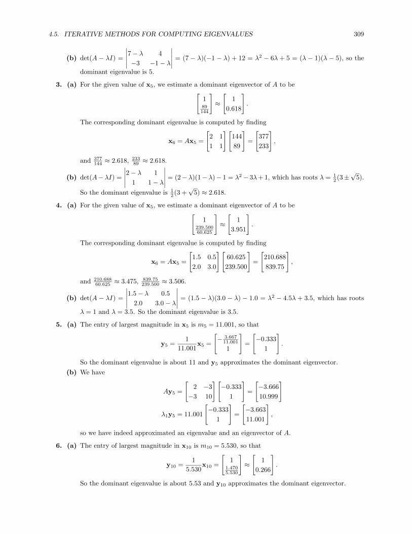
4.5. ITERATIVE METHODS FOR COMPUTING EIGENVALUES 309
(b) det(A − λI) =
∣∣∣∣∣7− λ 4
−3 −1− λ
∣∣∣∣∣ = (7 − λ)(−1 − λ) + 12 = λ2 − 6λ + 5 = (λ − 1)(λ − 5), so the
dominant eigenvalue is 5.
3. (a) For the given value of x5, we estimate a dominant eigenvector of A to be[189144
]≈
[1
0.618
].
The corresponding dominant eigenvalue is computed by finding
x6 = Ax5 =
[2 1
1 1
][144
89
]=
[377
233
],
and 377144 ≈ 2.618, 233
89 ≈ 2.618.
(b) det(A− λI) =
∣∣∣∣∣2− λ 1
1 1− λ
∣∣∣∣∣ = (2− λ)(1− λ)− 1 = λ2− 3λ+ 1, which has roots λ = 12 (3±
√5).
So the dominant eigenvalue is 12 (3 +
√5) ≈ 2.618.
4. (a) For the given value of x5, we estimate a dominant eigenvector of A to be[1
239.50060.625
]≈
[1
3.951
].
The corresponding dominant eigenvalue is computed by finding
x6 = Ax5 =
[1.5 0.5
2.0 3.0
][60.625
239.500
]=
[210.688
839.75
],
and 210.68860.625 ≈ 3.475, 839.75
239.500 ≈ 3.506.
(b) det(A − λI) =
∣∣∣∣∣1.5− λ 0.5
2.0 3.0− λ
∣∣∣∣∣ = (1.5 − λ)(3.0 − λ) − 1.0 = λ2 − 4.5λ + 3.5, which has roots
λ = 1 and λ = 3.5. So the dominant eigenvalue is 3.5.
5. (a) The entry of largest magnitude in x5 is m5 = 11.001, so that
y5 =1
11.001x5 =
[− 3.667
11.001
1
]=
[−0.333
1
].
So the dominant eigenvalue is about 11 and y5 approximates the dominant eigenvector.
(b) We have
Ay5 =
[2 −3
−3 10
][−0.333
1
]=
[−3.666
10.999
]
λ1y5 = 11.001
[−0.333
1
]=
[−3.663
11.001
],
so we have indeed approximated an eigenvalue and an eigenvector of A.
6. (a) The entry of largest magnitude in x10 is m10 = 5.530, so that
y10 =1
5.530x10 =
[1
1.4705.530
]≈
[1
0.266
].
So the dominant eigenvalue is about 5.53 and y10 approximates the dominant eigenvector.

310 CHAPTER 4. EIGENVALUES AND EIGENVECTORS
(b) We have
Ay10 =
[5 2
2 −2
][1
0.266
]=
[5.532
1.468
]
λ1y10 = 5.530
[1
0.266
]=
[5.530
1.471
],
so we have indeed approximated an eigenvalue and an eigenvector of A.
7. (a) The entry of largest magnitude in x8 is m8 = 10, so that
y8 =1
10x8 =
10.00110.0
1
≈ 1
0.0001
1
.So the dominant eigenvalue is about 10 and y8 approximates the dominant eigenvector.
(b) We have
Ay8 =
4 0 6
−1 3 1
6 0 4
1
0.0001
1
=
10
0.0003
10
λ1y8 = 10
1
0.0001
1
=
10
0.001
10
,so we have indeed approximated an eigenvalue and an eigenvector of A, though the approximationin the middle component is not great.
8. (a) The entry of largest magnitude in x10 is m10 = 3.415, so that
y10 =1
3.415x10 =
12.9143.415
− 1.2073.415
≈ 1
0.853
−0.353
.So the dominant eigenvalue is about 3.415 and y10 approximates the dominant eigenvector.
(b) We have
Ay10 =
1 2 −2
1 1 −3
0 −1 1
1
0.853
−0.353
=
3.412
2.912
−1.206
λ1y10 = 3.415
1
0.853
−0.353
=
3.415
2.913
−1.205
,so we have indeed approximated an eigenvalue and an eigenvector of A.
9. With the given A and x0, we get the values below:
k 0 1 2 3 4 5
xk
[11
] [268
] [17.6925.923
] [18.0176.004
] [17.9996.000
] [18.0006.000
]yk
[11
] [1.0000.308
] [1.0000.335
] [1.0000.333
] [1.0000.333
] [1.0000.333
]mk 1 26 17.692 18.017 17.999 18
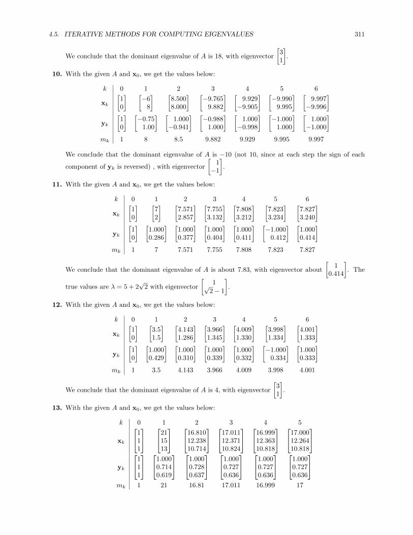
4.5. ITERATIVE METHODS FOR COMPUTING EIGENVALUES 311
We conclude that the dominant eigenvalue of A is 18, with eigenvector
[31
].
10. With the given A and x0, we get the values below:
k 0 1 2 3 4 5 6
xk
[10
] [−6
8
] [8.5008.000
] [−9.765
9.882
] [9.929−9.905
] [−9.990
9.995
] [9.997−9.996
]yk
[10
] [−0.75
1.00
] [1.000−0.941
] [−0.988
1.000
] [1.000−0.998
] [−1.000
1.000
] [1.000−1.000
]mk 1 8 8.5 9.882 9.929 9.995 9.997
We conclude that the dominant eigenvalue of A is −10 (not 10, since at each step the sign of each
component of yk is reversed) , with eigenvector
[1−1
].
11. With the given A and x0, we get the values below:
k 0 1 2 3 4 5 6
xk
[10
] [72
] [7.5712.857
] [7.7553.132
] [7.8083.212
] [7.8233.234
] [7.8273.240
]yk
[10
] [1.0000.286
] [1.0000.377
] [1.0000.404
] [1.0000.411
] [−1.000
0.412
] [1.0000.414
]mk 1 7 7.571 7.755 7.808 7.823 7.827
We conclude that the dominant eigenvalue of A is about 7.83, with eigenvector about
[1
0.414
]. The
true values are λ = 5 + 2√
2 with eigenvector
[1√
2− 1
].
12. With the given A and x0, we get the values below:
k 0 1 2 3 4 5 6
xk
[10
] [3.51.5
] [4.1431.286
] [3.9661.345
] [4.0091.330
] [3.9981.334
] [4.0011.333
]yk
[10
] [1.0000.429
] [1.0000.310
] [1.0000.339
] [1.0000.332
] [−1.000
0.334
] [1.0000.333
]mk 1 3.5 4.143 3.966 4.009 3.998 4.001
We conclude that the dominant eigenvalue of A is 4, with eigenvector
[31
].
13. With the given A and x0, we get the values below:
k 0 1 2 3 4 5
xk
111
211513
16.81012.23810.714
17.01112.37110.824
16.99912.36310.818
17.00012.26410.818
yk
111
1.0000.7140.619
1.0000.7280.637
1.0000.7270.636
1.0000.7270.636
1.0000.7270.636
mk 1 21 16.81 17.011 16.999 17

312 CHAPTER 4. EIGENVALUES AND EIGENVECTORS
We conclude that the dominant eigenvalue of A is 17, with corresponding eigenvector about
10.7270.636
.
In fact the eigenspace corresponding to this eigenvalue is span
120
, 0−2
1
, and we have found one
eigenvector in this space.
14. With the given A and x0, we get the values below:
k 0 1 2 3 4 5 6
xk
111
454
3.44.63.4
3.2174.4783.217
3.1554.4373.155
3.1334.4223.133
3.1264.4173.126
yk
111
0.81.00.8
0.7391.0000.739
0.7181.0000.718
0.7111.0000.711
0.7091.0000.709
0.7081.0000.708
mk 1 5 4.6 4.478 4.437 4.422 4.417
We conclude that the dominant eigenvalue of A is ≈ 4.4, with corresponding eigenvector ≈
0.7081.0000.708
.
In fact the dominant eigenvalue is 3 +√
2 with eigenspace spanned by
√
221√2
2
.
15. With the given matrix, and using x0 =
111
, we get
k 0 1 2 3 4 5 6 7 8 9
xk
111
824
5.750.502.25
5.260.171.87
5.100.071.74
5.040.031.70
5.020.011.68
5.010
1.67
50
1.67
50
1.67
yk
111
10.250.50
10.090.39
10.030.36
10.010.34
10.010.34
10
0.33
10
0.33
10
0.33
10
0.33
mk 1 8 5.75 5.26 5.10 5.04 5.02 5.01 5 5
We conclude that the dominant eigenvalue of A is 5, with corresponding eigenvector
301
.
16. With the given matrix, and using x0 =
111
, we get
k 0 1 2 3 4 5
xk
211
2426
11.01.5−2.5
14.182.45−7.91
16.383.12
−11.65
16.383.12
−11.65
yk
211
10.080.25
10.14−0.23
10.17−0.56
10.19−0.71
10.20−0.77
mk 2 24 11 14.18 16.38 17.41

4.5. ITERATIVE METHODS FOR COMPUTING EIGENVALUES 313
k 6 7 8 9 10 11
xk
17.803.54
−14.05
17.933.58
−14.28
17.983.59
−14.36
17.993.60
−14.39
18.003.60
−14.40
18.003.60
−14.40
yk
10.20−0.79
10.2−0.8
10.2−0.8
10.2−0.8
10.2−0.8
10.2−0.8
mk 17.8 17.93 17.98 17.99 18 18
We conclude that the dominant eigenvalue of A is 18, with corresponding eigenvector
10.2−0.8
, or 51−4
.
17. With the given A and x0, we get the values below:
k 0 1 2 3
xk
[10
] [72
] [7.5712.857
] [7.7553.132
]R(xk) 7 7.755 7.823 7.828
The Rayleigh quotient converges to the dominant eigenvalue, to three decimal places, after threeiterations.
18. With the given A and x0, we get the values below:
k 0 1 2 3
xk
[10
] [3.51.5
] [4.1431.286
] [3.9661.345
]R(xk) 3.5 3.966 3.998 4
The Rayleigh quotient converges to the dominant eigenvalue after three iterations.
19. With the given A and x0, we get the values below:
k 0 1 2
xk
111
211513
16.81012.23810.714
R(xk) 16.333 16.998 17
The Rayleigh quotient converges to the dominant eigenvalue after two iterations.
20. With the given A and x0, we get the values below:
k 0 1 2 3
xk
111
454
3.44.63.4
3.2174.4783.217
R(xk) 4.333 4.404 4.413 4.414
The Rayleigh quotient converges to the dominant eigenvalue, to three decimal places, after threeiterations.
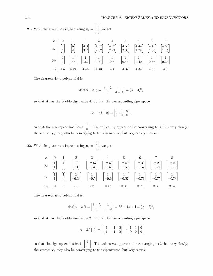
314 CHAPTER 4. EIGENVALUES AND EIGENVECTORS
21. With the given matrix, and using x0 =
[11
], we get
k 0 1 2 3 4 5 6 7 8
xk
[11
] [54
] [4.83.2
] [4.672.67
] [4.572.29
] [4.502.00
] [4.441.78
] [4.401.60
] [4.361.45
]
yk
[11
] [1
0.8
] [1
0.67
] [1
0.57
] [1
0.5
] [1
0.44
] [1
0.40
] [1
0.36
] [1
0.33
]mk 4.5 4.49 4.46 4.43 4.4 4.37 4.34 4.32 4.3
The characteristic polynomial is
det(A− λI) =
[4− λ 1
0 4− λ
]= (λ− 4)2,
so that A has the double eigenvalue 4. To find the corresponding eigenspace,
[A− 4I 0
]=
[0 1 00 0 0
],
so that the eigenspace has basis
[10
]. The values mk appear to be converging to 4, but very slowly;
the vectors yk may also be converging to the eigenvector, but very slowly if at all.
22. With the given matrix, and using x0 =
[11
], we get
k 0 1 2 3 4 5 6 7 8
xk
[11
] [40
] [3−1
] [2.67−1.33
] [2.50−1.50
] [2.40−1.60
] [2.33−1.67
] [2.29−1.71
] [2.25−1.70
]
yk
[11
] [10
] [1
−0.33
] [1−0.5
] [1−0.6
] [1
−0.67
] [1
−0.71
] [1
−0.75
] [1
−0.78
]mk 2 3 2.8 2.6 2.47 2.38 2.32 2.28 2.25
The characteristic polynomial is
det(A− λI) =
[3− λ 1−1 1− λ
]= λ2 − 4λ+ 4 = (λ− 2)2,
so that A has the double eigenvalue 2. To find the corresponding eigenspace,
[A− 2I 0
]=
[1 1 0−1 −1 0
]→[1 1 00 0 0
]
so that the eigenspace has basis
[1−1
]. The values mk appear to be converging to 2, but very slowly;
the vectors yk may also be converging to the eigenvector, but very slowly.

4.5. ITERATIVE METHODS FOR COMPUTING EIGENVALUES 315
23. With the given matrix, and using x0 =
111
, we get
k 0 1 2 3 4 5 6 7 8
xk
111
541
4.23.20.2
4.053.050.05
4.013.010.01
430
430
430
430
yk
111
10.80.2
10.760.05
10.750.01
10.75
0
10.75
0
10.75
0
10.75
0
10.75
0
mk 3.33 4.05 4.03 4.01 4 4 4 4 4
The matrix is upper triangular, so that A has an eigenvalue 1 and a double eigenvalue 4. To find theeigenspace for λ = 4,
[A− 4I 0
]=
0 0 1 00 0 0 00 0 −3 0
→0 0 1 0
0 0 0 00 0 0 0
so that the eigenspace has basis
1
00
,0
10
. The values mk converge to 4, while yk converge
apparently to
10.75
0
, which is in the eigenspace.
24. With the given matrix, and using x0 =
111
, we get
k 0 1 2 3 4 5 6 7 8
xk
111
065
05.834.17
05.713.57
05.623.12
05.562.78
05.502.50
05.452.27
05.422.08
yk
111
01
0.83
01
0.71
01
0.62
01
0.56
01
0.50
01
0.45
01
0.42
01
0.38
mk 3.67 5.49 5.47 5.45 5.42 5.4 5.38 5.36 5.34
The matrix is upper triangular, so that A has an eigenvalue 0 and a double eigenvalue 5. To find theeigenspace for λ = 5,
[A− 5I 0
]=
−5 0 0 00 0 1 00 0 0 0
→1 0 0 0
0 0 1 00 0 0 0
so that the eigenspace has basis
010
. The values mk appear to converge slowly to 5, while yk also
appear to converge slowly to
010
.

316 CHAPTER 4. EIGENVALUES AND EIGENVECTORS
25. With the given matrix, and using x0 =
[11
], we get
k 0 1 2 3 4
xk
[11
] [10
] [−1−1
] [10
] [−1−1
]
yk
[11
] [10
] [11
] [10
] [11
]mk 1 1 −1 1 −1
The characteristic polynomial is
det(A− λI) =
[−1− λ 2−1 1− λ
]= λ2 + 1,
so that A has no real eigenvalues, so the power method cannot succeed.
26. With the given matrix, and using x0 =
[11
], we get
k 0 1 2 3
xk
[11
] [33
] [33
] [33
]
yk
[11
] [11
] [11
] [11
]mk 1 3 3 3
The characteristic polynomial is
det(A− λI) =
[2− λ 1−2 5− λ
]= λ2 − 7λ+ 12 = (λ− 3)(λ− 4)
so that the power method converges to a non-dominant eigenvalue. This happened because we chose[11
]as the initial value, which is in fact an eigenvector for λ = 3:[
2 1−2 5
] [11
]=
[33
]= 3
[11
].
27. With the given matrix, and using x0 =
[11
], we get
k 0 1 2 3 4 5 6 7 8
xk
111
343
2.54.02.5
2.254
2.25
2.124
2.12
2.064
2.06
2.034
2.03
2.024
2.02
2.014
2.01
yk
111
0.751
0.75
0.621
0.62
0.561
0.56
0.531
0.53
0.521
0.52
0.511
0.51
0.51
0.5
0.51
0.5
mk 1 4 4 4 4 4 4 4 4
The characteristic polynomial is
det(A− λI) =
−5− λ 1 70 4− λ 07 1 −5− λ
= (λ+ 12)(λ− 4)(λ− 2)

4.5. ITERATIVE METHODS FOR COMPUTING EIGENVALUES 317
so that the power method converges to a non-dominant eigenvalue. This happened because we chose111
as the initial value. This vector is orthogonal to the eigenvector corresponding to the dominant
eigenvalue λ = −12, which is
10−1
:
−5 1 70 4 07 1 −5
10−1
=
−120
12
= −12
10−1
.28. With the given matrix, and using x0 =
[11
], we get
k 0 1 2 3 4 5 6 7 8
xk
111
021
−11−0.5
−20−2.5
0.80.81.8
00.89
1
−0.890.890.11
−20
−1.88
11
1.94
yk
111
01
0.5
−11−0.5
0.801
0.440.44
1
00.89
1
−11
0.12
10
0.94
0.520.52
1
mk 1 0.6 1.44 1.49 1 0.5 0.88 1.5 1
Neither mk nor yk shows clear signs of converging to anything. The characteristic polynomial is
det(A− λI) =
1− λ −1 01 1− λ 01 −1 1− λ
= (λ− 1)(λ2 − 2x+ 2)
so that A has eigenvalues 1 and 1± i. The absolute value of each of the complex eigenvectors is 2, so1 is not the eigenvalue of largest magnitude, and the power method cannot succeed.
29. In Exercise 9, we found that λ1 = 18. To find λ2, we apply the power method to
A− 18I =
[−4 12
5 −15
]with x0 =
[11
].
k 0 1 2 3
xk
[11
] [8
−10
] [15.2−19.0
] [15.2−19.0
]yk
[11
] [−0.8
1
] [−0.8
1
] [−0.8
1
]mk 1 −10 −19 −19
Thus λ2 − λ1 = −19, so that λ2 = −1 is the second eigenvalue of A.
30. In Exercise 10, we found that λ1 = −10, so we apply the power method to
A+ 10I =
[4 48 8
]with x0 =
[11
]:
k 0 1 2 3
xk
[11
] [816
] [612
] [612
]yk
[11
] [0.51
] [0.51
] [0.51
]mk 1 16 12 12
Thus λ2 − λ1 = 12, so that λ2 = 2 is the second eigenvalue of A.

318 CHAPTER 4. EIGENVALUES AND EIGENVECTORS
31. In Exercise 13, we found that λ1 = 17, so we apply the power method to
A− 17I =
−8 4 84 −2 −48 −4 −8
with x0 =
111
.k 0 1 2 3
xk
111
4−2−4
18−9−18
18−9−18
yk
111
−10.51
−10.51
−10.51
mk 1 −4 −18 −18
Thus λ2 − λ1 = −18, so that λ2 = −1 is the second eigenvalue of A.
32. In Exercise 14, we found that λ1 ≈ 4.4, so we apply the power method to
A− 4.4I =
−1.4 1 01 −1.4 10 1 −1.4
with x0 =
111
.k 0 1 2 3 4 5
xk
111
−0.40.6−0.4
1.933−2.733
1.933
1.990−2.815
1.990
1.990−2.814
1.990
1.990−2.814
1.990
yk
111
−0.6671
−0.667
−0.7071
−0.707
−0.7071
−0.707
−0.7071
−0.707
−0.7071
−0.707
mk 1 0.6 −2.733 −2.815 −2.814 −2.814
Thus λ2 − λ1 ≈ −2.81, so that λ2 ≈ 1.59 is the second eigenvalue of A (in fact, λ2 = 3−√
2).
33. With A and x0 as in Exercise 9, proceed to calculate xk by solving Axk = yk−1 at each step to applythe inverse power method. We get
k 0 1 2 3 4 5
xk
[11
] [0.5−0.5
] [0.833−1.056
] [0.798−0.997
] [0.8−1
] [0.8−1
]yk
[11
] [−1
1
] [−0.789
1
] [−0.801
1
] [−0.8
1
] [−0.8
1
]mk 1 −0.5 −1.056 −0.997 −1 −1
We conclude that the eigenvalue of A of smallest magnitude is 1−1 = −1.
34. With A and x0 as in Exercise 10, proceed to calculate xk by solving Axk = yk−1 at each step to applythe inverse power method. We get
k 0 1 2 3 4 5 6
xk
[11
] [0.10.4
] [0.2250.400
] [0.2560.525
] [0.2490.495
] [0.2500.501
] [0.250.50
]yk
[11
] [0.25
1
] [0.562
1
] [0.488
1
] [0.502
1
] [0.51
] [0.51
]mk 1 0.4 0.4 0.525 0.495 0.501 0.5
We conclude that the eigenvalue of A of smallest magnitude is 10.5 = 2.

4.5. ITERATIVE METHODS FOR COMPUTING EIGENVALUES 319
35. With A as in Exercise 7, and x0 as given, proceed to calculate xk by solving Axk = yk−1 at each stepto apply the inverse power method. We get
k 0 1 2 3 4 5 6
xk
11−1
−0.50
0.5
0.5000.333−0.500
0.5000.111−0.500
0.5000.259−0.500
0.500.16−0.50
yk
11−1
−101
−1−0.667
1
−1−0.222
1
−1−0.519
1
−1−0.321
1
mk −1 0.5 −0.5 −0.5 −0.5 −0.5
We conclude that the eigenvalue of A of smallest magnitude is 1−0.5 = −2.
36. With A and x0 as in Exercise 14, proceed to calculate xk by solving Axk = yk−1 at each step to applythe inverse power method. We get
k 0 1 2 3 4 5 6
xk
111
0.2860.1430.286
0.357−0.071
0.357
0.457−0.371
0.457
0.545−0.634
0.545
−0.5110.674−0.511
−0.4680.645−0.468
yk
111
10.51
1−0.2
1
1−0.812
1
−0.8591
−0.859
−0.7581
−0.758
−0.7251
−0.725
mk 1 0.286 0.357 0.457 −0.634 0.674 0.645
We conclude that the eigenvalue of A of smallest magnitude is ≈ 10.645 ≈ 1.55. In fact the eigenvalue
is 3−√
2.
37. With α = 0, we are just using the inverse power method, so the solution to Exercise 33 provides theeigenvalue closest to zero.
38. Since α = 0, there is no shift required, so this is the inverse power method. Take x0 = y0 =
[11
], and
proceed to calculate xk by solving Axk = yk−1 at each step to apply the inverse power method. Weget
k 0 1 2 3 4 5 6
xk
[11
] [0.1250.375
] [0.417−0.750
] [0.306−1.083
] [0.340−0.981
] [0.332−1.005
] [0.334−0.999
]yk
[11
] [0.333
1
] [−0.556
1
] [−0.282
1
] [−0.346
1
] [−0.33
1
] [−0.334
1
]mk 1 0.375 −0.75 −1.083 −0.981 −1.005 −0.999
We conclude that the eigenvalue of A closest to 0 (i.e., the eigenvalue smallest in magnitude) is 1−1 = −1.
39. We first shift A:
A− 5I =
−1 0 6−1 −2 1
6 0 −1
.Now take x0 = y0 =
111
, and proceed to calculate xk by solving Axk = yk−1 at each step to apply

320 CHAPTER 4. EIGENVALUES AND EIGENVECTORS
the inverse power method. We get
k 0 1 2 3
xk
111
0.2−0.5
0.2
−0.08−0.50−0.08
0.32−0.50
0.32
yk
111
−0.41−0.4
0.161
0.16
−0.0641
−0.064
mk 1 −0.5 −0.5 −0.5
We conclude that the eigenvalue of A closest to 5 is 5 + 1−0.5 = 3.
40. We first shift A:
A+ 2I =
11 4 74 17 −48 −4 11
.Now take x0 = y0 =
111
, and proceed to calculate xk by solving Axk = yk−1 at each step to apply
the inverse power method. We get
k 0 1 2 3 4 5
xk
111
−0.1580.1580.263
−0.8320.4320.853
−0.9900.4960.991
−0.9990.5001.000
−10.51
yk
111
−0.60.61
−0.9750.506
1
−0.9990.51
−10.51
−10.51
mk 1 0.263 0.853 0.991 1 1
We conclude that the eigenvalue of A closest to −2 is −2 + 11 = −1.
41. The companion matrix of p(x) = x2 + 2x− 2 is
C(p) =
[−2 2
1 0
],
so we apply the inverse power method with x0 = y0 =
[11
], calculating xk by solving Axk = yk−1 at
each step. We get
k 0 1 2 3 4 5 6
xk
[11
] [1
1.5
] [1
1.333
] [1
1.375
] [1
1.364
] [1
1.367
] [1
1.366
]yk
[11
] [0.667
1
] [0.75
1
] [0.727
1
] [0.733
1
] [0.732
1
] [0.732
1
]mk 1 1.5 1.333 1.375 1.364 1.367 1.366
So the root of p(x) closest to 0 is ≈ 11.366 ≈ 0.732. The exact value is −1 +
√3.
42. The companion matrix of p(x) = x2 − x− 3 is
C(p) =
[1 31 0
],

4.5. ITERATIVE METHODS FOR COMPUTING EIGENVALUES 321
so we apply the inverse power method to
C(p)− 2I =
[−1 3
1 −2
]with x0 = y0 =
[11
], calculating xk by solving Axk = yk−1 at each step. We get
k 0 1 2 3 4 5 6
xk
[11
] [52
] [3.21.4
] [3.3121.438
] [3.3021.434
] [3.3031.434
] [3.3031.434
]yk
[11
] [1
0.4
] [1
0.438
] [1
0.434
] [1
0.434
] [1
0.434
] [1
0.434
]mk 1 5 3.2 3.312 3.302 3.303 3.303
So the root of p(x) closest to 2 is ≈ 2 + 13.303 ≈ 2.303. The exact value is 1
2 (1 +√
13).
43. The companion matrix of p(x) = x3 − 2x2 + 1 is
C(p) =
2 0 −11 0 00 1 0
,so we apply the inverse power method to C(p). If we first start with y0 =
111
, we find that this is an
eigenvector of C(p) with eigenvalue 1, but this may not be the closest root to 0, so we start instead
with with x0 = y0 =
101
, calculating xk by solving Axk = yk−1 at each step. We get
k 0 1 2 3 4 5
xk
101
01−1
−11−2
−0.51
0.5
−0.6671
−1.667
−0.61−1.6
yk
101
0−1
1
0.5−0.5
1
0.333−0.667
1
0.4−0.6
1
0.375−0.625
1
mk 1 −1 −2 −1.6 −1.667 −1.6
k 6 7 8 9
xk
−0.6251
−1.625
−0.6151
−1.615
−0.6191
1.619
−0.6181
−1.618
yk
0.385−0.615
1
0.381−0.619
1
0.382−0.618
1
0.382−0.618
1
mk −1.625 −1.615 −1.619 −1.618
We conclude that the root of p(x) closest to zero is 1−1.618 ≈= −0.618. The actual root is 1
2 (1−√
5).
44. The companion matrix of p(x) = x3 − 2x2 + 1 is
C(p) =
5 −1 −11 0 00 1 0
,
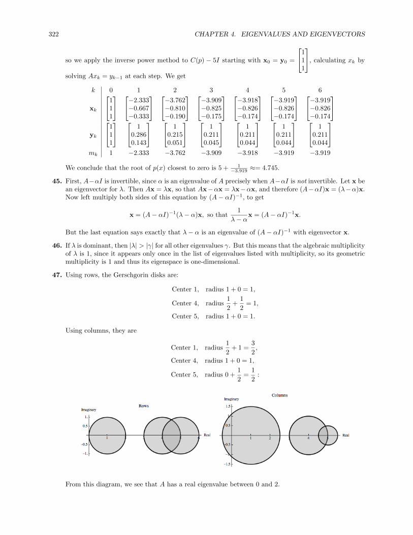
322 CHAPTER 4. EIGENVALUES AND EIGENVECTORS
so we apply the inverse power method to C(p) − 5I starting with x0 = y0 =
111
, calculating xk by
solving Axk = yk−1 at each step. We get
k 0 1 2 3 4 5 6
xk
111
−2.333−0.667−0.333
−3.762−0.810−0.190
−3.909−0.825−0.175
−3.918−0.826−0.174
−3.919−0.826−0.174
−3.919−0.826−0.174
yk
111
10.2860.143
10.2150.051
10.2110.045
10.2110.044
10.2110.044
10.2110.044
mk 1 −2.333 −3.762 −3.909 −3.918 −3.919 −3.919
We conclude that the root of p(x) closest to zero is 5 + 1−3.919 ≈= 4.745.
45. First, A−αI is invertible, since α is an eigenvalue of A precisely when A−αI is not invertible. Let x bean eigenvector for λ. Then Ax = λx, so that Ax−αx = λx−αx, and therefore (A−αI)x = (λ−α)x.Now left multiply both sides of this equation by (A− αI)−1, to get
x = (A− αI)−1(λ− α)x, so that1
λ− αx = (A− αI)−1x.
But the last equation says exactly that λ− α is an eigenvalue of (A− αI)−1 with eigenvector x.
46. If λ is dominant, then |λ| > |γ| for all other eigenvalues γ. But this means that the algebraic multiplicityof λ is 1, since it appears only once in the list of eigenvalues listed with multiplicity, so its geometricmultiplicity is 1 and thus its eigenspace is one-dimensional.
47. Using rows, the Gerschgorin disks are:
Center 1, radius 1 + 0 = 1,
Center 4, radius1
2+
1
2= 1,
Center 5, radius 1 + 0 = 1.
Using columns, they are
Center 1, radius1
2+ 1 =
3
2,
Center 4, radius 1 + 0 = 1,
Center 5, radius 0 +1
2=
1
2:
From this diagram, we see that A has a real eigenvalue between 0 and 2.

4.5. ITERATIVE METHODS FOR COMPUTING EIGENVALUES 323
48. Using rows, the Gerschgorin disks are:
Center 2, radius |−i|+ 0 = 1,
Center 2i, radius |1|+ |1 + i| = 1 +√
2,
Center − 2i, radius 0 + 1 = 1.
Using columns, they are
Center 2, radius 1 + 0 = 1,
Center 2i, radius |−i|+ 1 = 2,
Center − 2i, radius 0 + |1 + i| =√
2 :
From this diagram, we conclude that A has an eigenvalue within one unit of −2i.
49. Using rows, the Gerschgorin disks are:
Center 4− 3i, radius |i|+ 2 + 2 = 5,
Center − 1 + i, radius |i|+ 0 + 0 = 1,
Center 5 + 6i, radius |1 + i|+ |−i|+ |2i| = 3 +√
2
Center − 5− 5i, radius 1 + |−2i|+ |2i| = 5.
Using columns, they are
Center 4− 3i, radius |i|+ |1 + i|+ 1 = 2 +√
2,
Center − 1 + i, radius |i|+ |−i|+ |−2i| = 4,
Center 5 + 6i, radius 2 + 0 + |2i| = 4
Center − 5− 5i, radius |−2|+ 0 + |2i| = 4.

324 CHAPTER 4. EIGENVALUES AND EIGENVECTORS
From this diagram, we conclude that A has an eigenvalue within 1 unit of −1 + i.
50. Using rows, the Gerschgorin disks are:
Center 2, radius1
2,
Center 4, radius1
4+
1
4=
1
2,
Center 6, radius1
6+
1
6=
2
3
Center 8, radius1
8.
Using columns, they are
Center 2, radius1
4,
Center 4, radius1
2+
1
6=
1
3,
Center 6, radius1
4+
1
8=
3
8
Center 8, radius1
6.
Since the circles are all disjoint, we conclude that A has four real eigenvalues, near 2, 4, 6, and 8.
51. Let A be a strictly diagonally dominant square matrix. Then in particular, none of the diagonal entriesof A can be zero, since each row has the property that |aii| >
∑j 6=i |aij |. Therefore each Gerschgorin
disk is centered at a nonzero point, and its radius is less than the absolute value of its center, so the diskdoes not contain the origin. Since every eigenvalue is contained in some Gerschgorin disk, it followsthat 0 is not an eigenvalue, so that the matrix is invertible by Theorem 4.17.

4.5. ITERATIVE METHODS FOR COMPUTING EIGENVALUES 325
52. Let λ be any eigenvalue of A. Then by Theorem 4.29, λ is contained in the Gerschgorin disk for somerow i, so that
|λ− aii| ≤∑j 6=i
|aij | .
By the Triangle Inequality, |λ| ≤ |λ− aii|+ |aii|, so that
|λ| ≤ |λ− aii|+ |aii| ≤ |aii|+∑j 6=i
|aij | =n∑j=1
|aij | ≤ ‖A‖ ,
since ‖A‖ is the maximum of the possible row sums.
53. A stochastic matrix is a square matrix whose entries are probability vectors, which means that thesum of the entries in any column of A is 1, so the sum of the entries of any row in AT is 1, so that∥∥AT∥∥ = 1. By Exercise 52, any eigenvalue of AT must satisfy |λ| ≤
∥∥AT∥∥ = 1. But by Exercise 19in Section 4.3, the eigenvalues of A and of AT are the same, so that if λ is any eigenvalue of A, then|λ| ≤ 1.
54. Using rows, the Gerschgorin disks are:
Center 0, radius 1,
Center 5, radius 2,
Center 3, radius1
2+
1
2= 1
Center 7, radius3
4.
Using columns, they are
Center 0, radius 2 +1
2=
5
2,
Center 5, radius 1,
Center 3, radius3
4
Center 7, radius1
2.
From the row diagram, we see that there is exactly one eigenvalue in the circle of radius 1 around 0, soit must be real and therefore there is exactly one eigenvalue in the interval [−1, 1]. From the columndiagram, we similarly conclude that there is exactly one eigenvalue in the interval [4, 6] and exactlyone in
[132 ,
152
].
Since the matrix has real entries, the fourth eigenvalue must be real as well. From the row diagram,since the circle around zero contains exactly one eigenvalue, the fourth eigenvalue must be in theinterval
[2, 7 3
4
]. But it cannot be larger than 3 3
4 since then, from the column diagram, it would either

326 CHAPTER 4. EIGENVALUES AND EIGENVECTORS
not be in a disk or would be in an isolated disk already containing an eigenvalue. So it must lie in therange
[2, 3 3
4
].
In summary, the four eigenvalues are each in a different one of the four intervals
[−1, 1], [2, 3.75], [4, 6], [6.5, 7.5].
The actual values are ≈ −0.372, ≈ 2.908, ≈ 5.372, and ≈ 7.092.
4.6 Applications and the Perron-Frobenius Theorem
1. Since
[0 11 0
]2
=
[1 00 1
], it follows that any power of
[0 11 0
]contains zeroes. So this matrix is not
regular.
2. Since the given matrix is upper triangular, any of its powers is upper triangular as well, so will containa zero. Thus this matrix is not regular.
3. Since [13 123 0
]2
=
[79
13
29
23
],
the square of the given matrix has all positive entries, so this matrix is regular.
4. We have 12 0 112 0 0
0 1 0
2
=
14 1 1
214 0 1
212 0 0
12 0 112 0 0
0 1 0
3
=
12 0 112 0 0
0 1 0
14 1 1
214 0 1
212 0 0
=
58
12
14
18
12
14
14 0 1
2
12 0 112 0 0
0 1 0
4
=
12 0 112 0 0
0 1 0
58
12
14
18
12
14
14 0 1
2
=
916
14
58
516
14
18
18
12
14
so that the fourth power of this matrix contains all positive entries, so this matrix is regular.
5. If A and B are any 3× 3 matrices with a12 = a32 = b12 = b32 = 0, then
(AB)12 = a11b12 +a12b22 +a13b32 = 0 + 0 + 0 = 0, (AB)32 = a31b12 +a32b22 +a33b32 = 0 + 0 + 0 = 0,
so that AB has the same property. Thus any power of the given matrix A has this property, so nopower of A consists of positive entries, so A is not regular.
6. Since the third row of the matrix is all zero, the third row of any power will also be all zero, so thismatrix is not regular.
7. The transition matrix P has characteristic equation
det(P − λI) =
∣∣∣∣∣ 13 − λ 16
23
56 − λ
∣∣∣∣∣ =1
6(λ− 1)(6λ− 1),
so its eigenvalues are λ1 = 1 and λ2 = 16 . Thus P has two distinct eigenvalues, so is diagonalizable.
Now, this matrix is regular, so the remark at the end of the proof of Theorem 4.33 shows that the

4.6. APPLICATIONS AND THE PERRON-FROBENIUS THEOREM 327
vector x which forms the columns of L is a probability vector parallel to an eigenvector for λ = 1. Tocompute this, we row-reduce P − I:
[P − I 0
]=
[− 2
316 0
23 − 1
6 0
]→
[1 − 1
4 0
0 0 0
]
so that the corresponding eigenspace is
E1 = span
([14
]).
Thus the columns of L are of the form
[t4t
]where t+ 4t = 5t = 1, so that t = 1
5 . Therefore
L =
[15
15
45
45
].
8. The transition matrix P has characteristic equation
det(P − λI) =
∣∣∣∣∣∣∣12 − λ
13
16
12
12 − λ
13
0 16
12 − λ
∣∣∣∣∣∣∣ = − 1
36(λ− 1)(36λ2 − 18λ+ 1).
So one eigenvalue is 1; the roots of the quadratic are distinct, so that P has three distinct eigenvalues,so is diagonalizable. Now, this matrix is regular (its square has all positive entries), so the remarkat the end of the proof of Theorem 4.33 shows that the vector x which forms the columns of L is aprobability vector parallel to an eigenvector for λ = 1. To compute this, we row-reduce P − I:
[P − I 0
]=
−12
13
16 0
12 − 1
213 0
0 16 − 1
2 0
→1 0 − 7
3 0
0 1 −3 0
0 0 0 0
so that the corresponding eigenspace is
E1 = span
793
.
Thus the columns of L are of the form
7t9t3t
where 7t+ 9t+ 3t = 19t = 1, so that t = 119 . Therefore
L =1
19
7 7 79 9 93 3 3
.9. The transition matrix P has characteristic equation
det(P − λI) =
∣∣∣∣∣∣∣0.2− λ 0.3 0.4
0.6 0.1− λ 0.4
0.2 0.6 0.2− λ
∣∣∣∣∣∣∣ = −(λ− 1)(λ2 + 0.5λ+ 0.08)
So one eigenvalue is 1; the roots of the quadratic are distinct (and complex), so that P has threedistinct eigenvalues, so is diagonalizable. Now, this matrix is regular, so the remark at the end of the

328 CHAPTER 4. EIGENVALUES AND EIGENVECTORS
proof of Theorem 4.33 shows that the vector x which forms the columns of L is a probability vectorparallel to an eigenvector for λ = 1. To compute this, we row-reduce P − I:
[P − I 0
]=
−0.8 0.3 0.4 0
0.6 −0.9 0.4 0
0.2 0.6 −0.8 0
→1 0 −0.889 0
0 1 −1.037 0
0 0 0 0
so that the corresponding eigenspace is
E1 = span
0.8891.037
1
.
Thus the columns of L are of the form
0.889t1.037t
1t
where 0.889t + 1.037t + t = 2.926t = 1, so that
t = 12.926 . Therefore
L =
0.304 0.304 0.3040.354 0.354 0.3540.341 0.341 0.341
.(If the matrix is converted to fractions and the computation done that way, the resulting eigenvector
will be
242827
, which must then be converted to a unit vector.)
10. Suppose that the sequence of iterates xk approach both u and v, and choose ε > 0. Choose k suchthat |xk − u| < ε
2 and |xk − v| < ε2 . Then
|u− v| = |(u− xk) + (xk − v)| ≤ |u− xk|+ |xk − v| < ε,
so that |u− v| is less than any positive ε. So it must be zero; that is, we must have u = v.
11. The characteristic polynomial is
det(L− λI) =
∣∣∣∣−λ 20.5 −λ
∣∣∣∣ = λ2 − 1 = (λ+ 1)(λ− 1),
so the positive eigenvalue is 1. To find a corresponding eigenvector, row-reduce
[L− I 0
]=
[−1 2 00.5 −1 0
]→[1 −2 00 0 0
].
Thus E1 = span
([21
]).
12. The characteristic polynomial is
det(L− λI) =
∣∣∣∣1− λ 1.50.5 −λ
∣∣∣∣ = λ2 − λ− 0.75 = (λ− 1.5)(λ+ 0.5),
so the positive eigenvalue is 1.5. To find a corresponding eigenvector, row-reduce
[L− 1.5I 0
]=
[−0.5 1.5 0
0.5 −1.5 0
]→[1 −3 00 0 0
].
Thus E1.5 = span
([31
]).

4.6. APPLICATIONS AND THE PERRON-FROBENIUS THEOREM 329
13. The characteristic polynomial is
det(L− λI) =
∣∣∣∣∣∣−λ 7 40.5 −λ 00 0.5 −λ
∣∣∣∣∣∣ = −λ3 + 3.5λ+ 1 = −1
2(λ− 2)(2λ2 + 4λ+ 1),
so 2 is a positive eigenvalue. The other two roots are
−4±√
8
4,
both of which are negative. To find an eigenvector for 2, row-reduce
[L− 2I 0
]=
−2 7 4 00.5 −2 0 0
0 0.5 −2 0
→1 0 −16 0
0 1 −4 00 0 0 0
.
Thus E2 = span
1641
.
14. The characteristic polynomial is
det(L− λI) =
∣∣∣∣∣∣∣1− λ 5 3
13 −λ 0
0 23 −λ
∣∣∣∣∣∣∣ = −x3 + x2 +5
3x+
2
3= −1
3(x− 2)(3x2 + 3x+ 1)
so 2 is a positive eigenvalue. The other two eigenvalues are complex. To find an eigenvector for 2,row-reduce [
L− 2I 0]
=
−1 5 3 013 −2 0 0
0 23 −2 0
→1 0 −18 0
0 1 −3 0
0 0 0 0
.
Thus E2 = span
1831
.
15. Since the eigenvector corresponding to the positive eigenvalue λ1 for the Leslie matrix represents astable ratio of population classes, one that proportion is reached, if λ1 > 1, the population will growwithout bound; if λ1 = 1, it will be stable, and if λ1 < 1 it will decrease and eventually die out.
16. From the Leslie matrix in Equation (3), we have
det(L− λI) =
∣∣∣∣∣∣∣∣∣∣∣∣∣
b1 − λ b2 b3 · · · bn−1 bns1 −λ 0 · · · 0 00 s2 −λ · · · 0 00 0 s3 · · · 0 0...
......
. . ....
...0 0 0 · · · sn−1 −λ
∣∣∣∣∣∣∣∣∣∣∣∣∣.
For n = 1, this is just b1 − λ, which is equal to
cL(λ) = (−1)1(λ1 − b1λ0) = b1 − λ.

330 CHAPTER 4. EIGENVALUES AND EIGENVECTORS
This forms the basis for the induction. Now assume the statement holds for n− 1, and we prove it forn. Expand the above determinant along the last column, giving
det(L− λI) = (−1)n+1bn
∣∣∣∣∣∣∣∣∣∣∣
s1 −λ 0 · · · 00 s2 −λ · · · 00 0 s3 · · · 0...
......
. . ....
0 0 0 · · · sn−1
∣∣∣∣∣∣∣∣∣∣∣+ (−λ)
∣∣∣∣∣∣∣∣∣∣∣∣∣
b1 − λ b2 b3 · · · bn−2 bn−1
s1 −λ 0 · · · 0 00 s2 −λ · · · 0 00 0 s3 · · · 0 0...
......
. . ....
...0 0 0 · · · sn−2 0
∣∣∣∣∣∣∣∣∣∣∣∣∣.
The first matrix is upper triangular, so its determinant is the product of its diagonal entries; for thesecond, we use the inductive hypothesis. So
det(L− λI) = (−1)n+1bn(s1s2 · · · sn−1)
− λ((−1)n−1(λn−1 − b1λn−2 − b2s1λ
n−3 − · · ·−bn−2s1s2 · · · sn−3λ− bn−1s1s2 · · · sn−2)
= (−1)n+1bn(s1s2 · · · sn−1)
+ (−1)n(λn − b1λn−1 − b2s1λn−2 − · · ·
− bn−2s1s2 · · · sn−3λ2 − bn−1s1s2 · · · sn−2λ)
= (−1)n(λn − b1λn−1 − b2s1λn−2 − · · ·
− bn−2s1s2 · · · sn−3λ2 − bn−1s1s2 · · · sn−2λ− bns1s2 · · · sn−1),
proving the result.
17. P is a diagonal matrix, so inverting it consists of inverting each of the diagonal entries. Now, multiplyingany matrix on the left by a diagonal matrix multiplies each row by the corresponding diagonal entry,and multiplying on the right by a diagonal matrix multiplies each column by the corresponding diagonalentry, so
P−1L =
b1 b2 b3 · · · bn−1 bn
1 0 0 · · · 0 0
0 1s1
0 · · · 0 0
0 0 1s1s2
· · · 0 0...
......
. . ....
...
0 0 0 · · · 1s1s2···sn−2
0
and then
P−1LP =
b1 b2s1 b3s1s2 · · · bn−1s1s2 · · · sn−2 bns1s2 · · · sn−1
1 0 0 · · · 0 0
0 1 0 · · · 0 0
0 0 1 · · · 0 0...
......
. . ....
...
0 0 0 · · · 1 0
.
But this is the companion matrix of the polynomial
p(x) = xn − b1xn−1 − b2s1xn−2 − · · · − bn−1s1s2 · · · sn−2x− bns1s2 · · · sn−1,
and by Exercise 32 in Section 4.3, the characteristic polynomial of P−1LP is (−1)np(λ). Finally, thecharacteristic polynomials of L and P−1LP are the same since they have the same eigenvalues, so thecharacteristic polynomial of L is
det(L− λI) = det(P−1LP − λI) = (−1)np(λ)
= (−1)n(λn − b1λn−1 − b2s1λn−2 − · · · − bn−1s1s2 · · · sn−2λ− bns1s2 · · · sn−1)

4.6. APPLICATIONS AND THE PERRON-FROBENIUS THEOREM 331
18. By Exercise 46 in Section 4.4, the eigenvectors of P−1LP are of the form P−1x where x is an eigenvalueof L, and by Exercise 32 in Section 4.3, an eigenvector of P−1LP for λ1 is
λn−11
λn−21
λn−31...λ1
1
.
So an eigenvector of L corresponding to λ1 is
P
λn−11
λn−21
λn−31...λ1
1
=
λn−11
s1λn−21
s1s2λn−31
...s1s2 · · · sn−2λ1
s1s2 · · · sn−2sn−1
.
Finally, we can scale this vector by dividing each entry by λn−11 to get
1s1/λ1
s1s2/λ21
...s1s2 · · · sn−2/λ
n−21
s1s2 · · · sn−2sn−1/λn−11
.
19. Using a CAS, we find the positive eigenvalue of
L =
1 1 30.7 0 00 0.5 0
to be λ ≈ 1.7456, so this is the steady state growth rate of the population with this Leslie matrix.From Exercise 18, a corresponding eigenvector is 1
0.7/1.74560.7 · 0.5/(1.7456)2
≈ 1
0.4010.115
.So the long-term proportions of the age classes are in the ratios 1 : 0.401 : 0.115.
20. Using a CAS, we find the positive eigenvalue of
L =
0 1 2 5
0.5 0 0 00 0.7 0 00 0 0.3 0
to be λ ≈ 1.2023, so this is the steady state growth rate of the population with this Leslie matrix.From Exercise 18, a corresponding eigenvector is
10.5/1.2023
0.5 · 0.7/(1.2023)2
0.5 · 0.7 · 0.3/(1.2023)3
≈
10.4160.2420.060
So the long-term proportions of the age classes are in the ratios 1 : 0.416 : 0.242 : 0.06.

332 CHAPTER 4. EIGENVALUES AND EIGENVECTORS
21. Using a CAS, we find the positive eigenvalue of
L =
0 0.4 1.8 1.8 1.8 1.6 0.60.3 0 0 0 0 0 00 0.7 0 0 0 0 00 0 0.9 0 0 0 00 0 0 0.9 0 0 00 0 0 0 0.9 0 00 0 0 0 0 0.6 0
.
to be λ ≈ 1.0924, so this is the steady state growth rate of the population with this Leslie matrix.From Exercise 18, a corresponding eigenvector is
10.3/1.0924
0.3 · 0.7/(1.0924)2
0.3 · 0.7 · 0.9/(1.0924)3
0.3 · 0.7 · 0.9 · 0.9/(1.0924)4
0.3 · 0.7 · 0.9 · 0.9 · 0.9/(1.0924)5
0.3 · 0.7 · 0.9 · 0.9 · 0.9 · 0.6/(1.0924)6
≈
10.2750.1760.1450.1190.0980.054
.
The entries of this vector give the long-term proportions of the age classes.
22. (a) The table gives us 13 separate age classes, each of duration two years; from the table, the Lesliematrix of the system is
L =
0 0.02 0.70 1.53 1.67 1.65 1.56 1.45 1.22 0.91 0.70 0.22 00.91 0 0 0 0 0 0 0 0 0 0 0 0
0 0.88 0 0 0 0 0 0 0 0 0 0 00 0 0.85 0 0 0 0 0 0 0 0 0 00 0 0 0.80 0 0 0 0 0 0 0 0 00 0 0 0 0.74 0 0 0 0 0 0 0 00 0 0 0 0 0.67 0 0 0 0 0 0 00 0 0 0 0 0 0.59 0 0 0 0 0 00 0 0 0 0 0 0 0.49 0 0 0 0 00 0 0 0 0 0 0 0 0.38 0 0 0 00 0 0 0 0 0 0 0 0 0.27 0 0 00 0 0 0 0 0 0 0 0 0 0.17 0 00 0 0 0 0 0 0 0 0 0 0 0.15 0
.
Using a CAS, this matrix has positive eigenvalue ≈ 1.333, with a corresponding eigenvector(normalized to add to 100)
36.124.6516.2710.386.233.461.740.770.280.080.0160.00210.00023
.

4.6. APPLICATIONS AND THE PERRON-FROBENIUS THEOREM 333
(b) In the long run, the percentage of seals in each age group is given by the entries in the eigenvectorin part (a), and the growth rate will be about 1.333.
23. (a) Each term in r is the number of daughters born to a female in a particular age class times theprobability of a given individual surviving to be in that age class, so it represents the expectednumber of daughters produced by a given individual while she is in that age class. So the sumof the terms gives the expected number of daughters ever born to a particular female over herlifetime.
(b) Define g(λ) as suggested. Then g(λ) = 1 if and only if
λng(λ) = b1λn−1 + b2s1λ
n−2 + · · ·+ bns1s2 · · · sn−1 = λn ⇒λn − b1λn−1 − b2s1λ
n−2 − · · · − bns1s2 · · · sn−1 = 0.
But from Exercise 16, this is true if and only if λ is a zero of the characteristic polynomial of theLeslie matrix, indicating that λ is an eigenvalue of L. So r = g(1) = 1 if and only if λ = 1 is aneigenvalue of L, as desired.
(c) For given values of bi and si, it is clear that g(λ) is a decreasing function of λ. Also, r = g(1) andg(λ1) = 1. So if λ1 > 1, then r = g(1) > g(λ1) = 1 so that r > 1. On the other hand, if λ1 < 1,then r = g(1) < g(λ1) = 1, so that r < 1. So we have shown that if the population is decreasing,then r < 1; if the population is increasing, then r > 1, and (part (b)) if the population is stable,then r = 1. Since this exhausts the possibilities, we have proven the converses as well. Thus r < 1if and only if the population is decreasing and r > 1 if and only if the population is increasing.Note that this corresponds to our intuition, since if the net reproduction rate is less than one, wewould expect the population in the next generation to be smaller.
24. If λ1 is the unique positive eigenvalue, then λ1x = Lx for the corresponding eigenvector x. If h is thesustainable harvest ratio, then (1− h)Lx = x, which means that Lx = 1
1−hx. Thus λ1 = 11−h , so that
h = 1− 1λ1
.
25. (a) Exercise 21 found the positive eigenvalue of L to be λ1 ≈ 1.0924, so from Exercise 24, h = 1− 1λ1≈
1− 11.0924 ≈ 0.0846.
(b) Reducing the initial population levels by 0.0846 gives
x′0 = (1− 0.0846)
102851201
=
9.151.8317.3234.57710.985
00.915
.
Then
x′1 = Lx′0 =
0 0.4 1.8 1.8 1.8 1.6 0.60.3 0 0 0 0 0 00 0.7 0 0 0 0 00 0 0.9 0 0 0 00 0 0 0.9 0 0 00 0 0 0 0.9 0 00 0 0 0 0 0.6 0
9.151.8317.3234.57710.985
00.915
=
42.472.751.286.594.129.89
0
.
The population has still grown substantially, because we did not start with a stable population

334 CHAPTER 4. EIGENVALUES AND EIGENVECTORS
vector. If we repeat with the stable population ratios computed in Exercise 21, we get
x′0 = (1− 0.0846)
10.2750.1760.1450.1190.0980.054
=
0.9150.2520.1610.1330.1090.0900.049
,
and
x′1 = Lx′0 =
0 0.4 1.8 1.8 1.8 1.6 0.60.3 0 0 0 0 0 00 0.7 0 0 0 0 00 0 0.9 0 0 0 00 0 0 0.9 0 0 00 0 0 0 0.9 0 00 0 0 0 0 0.6 0
0.9150.2520.1610.1330.1090.0900.049
=
0.9990.2750.1760.1450.1190.0980.053
,
which is essentially x0.
26. Since λ1 ≈ 1.333, we have h = 1− 1λ1
= 1− 11.333 ≈ 0.25, which is about one quarter of the population.
27. Suppose λ1 = r1(cos 0 + i sin 0); then r1 = λ1 > 0 since λ1 is a positive eigenvalue. Let λ = r(cos θ +i sin θ) be some other eigenvalue. Then g(λ) = g(λ1) = 1. Computing g(λ) gives
1 = g(λ) =b1
r(cos θ + i sin θ)+
b2s1
r2(cos θ + i sin θ)2+ · · ·+ bns1s2 · · · sn−1
rn(cos θ + i sin θ)n
=b1r
(cos θ − i sin θ) +b2s1
r2(cos θ − i sin θ)2 + · · ·+ b2s1s2 · · · sn−1
rn(cos θ − i sin θ)n,
where we get to the final equation by multiplying each fraction by (cos θ−i sin θ)k
(cos θ−i sin θ)k= 1 and using the
identity (cos θ + i sin θ)(cos θ − i sin θ) = cos2 θ + sin2 θ = 1. Now apply DeMoivre’s theorem to get
1 = g(λ) =b1r
(cos θ − i sin θ) +b2s1
r2(cos 2θ − i sin 2θ) + · · ·+ b2s1s2 · · · sn−1
rn(cosnθ − i sinnθ).
Since g(λ) = 1, the imaginary parts must all cancel, so we are left with
1 = g(λ) =b1r
cos θ +b2s1
r2cos 2θ + · · ·+ b2s1s2 · · · sn−1
rncosnθ.
But cos kθ ≤ 1 for all k, and bi, si, and r are all nonnegative, so
1 = g(λ) ≤ b1r
+b2s1
r2+ · · ·+ b2s1s2 · · · sn−1
rn.
Since g(λ1) = 1 as well, we get
b1r1
+b2s1
r21
+ · · ·+ b2s1s2 · · · sn−1
rn1≤ b1
r+b2s1
r2+ · · ·+ b2s1s2 · · · sn−1
rn.
Then since r1 > 0, we get r1 ≥ r.
28. The characteristic polynomial of A is
det(A− λI) =
∣∣∣∣2− λ 01 1− λ
∣∣∣∣ = (λ− 2)(λ− 1),

4.6. APPLICATIONS AND THE PERRON-FROBENIUS THEOREM 335
so that the Perron root is λ1 = 2. To find its Perron eigenvector,
[A− 2I 0
]=
[0 0 01 −1 0
]→[1 −1 00 0 0
],
so that
[11
]is an eigenvector for λ1 = 2. The entries of the Perron eigenvector must sum to 1, however,
so dividing through by 2 gives for the Perron eigenvector
[1212
].
29. The characteristic polynomial of A is
det(A− λI) =
∣∣∣∣1− λ 32 −λ
∣∣∣∣ = (1− λ)(−λ)− 6 = λ2 − λ− 6 = (λ− 3)(λ+ 2),
so that the Perron root is λ1 = 3. To find its Perron eigenvector,
[A− 3I 0
]=
[−2 3 0
2 −3 0
]→
[1 − 3
2 0
0 0 0
],
so that
[32
]is an eigenvector for λ1 = 3. The entries of the Perron eigenvector must sum to 1, however,
so dividing through by 5 gives for the Perron eigenvector
[3525
].
30. The characteristic polynomial of A is
det(A− λI) =
∣∣∣∣∣∣−λ 1 11 −λ 11 1 −λ
∣∣∣∣∣∣ = −(λ+ 1)2(λ− 2),
so that the Perron root is λ1 = 2. To find its Perron eigenvector,
[A− 2I 0
]=
−2 1 1 0
1 −2 1 0
1 1 −2 0
→1 0 −1 0
0 1 −1 0
0 0 0 0
,
so that
111
is an eigenvector for λ1 = 2. The entries of the Perron eigenvector must sum to 1, however,
so dividing through by 3 gives for the Perron eigenvector
131313
.
31. The characteristic polynomial of A is
det(A− λI) =
∣∣∣∣∣∣2− λ 1 1
1 1− λ 01 0 1− λ
∣∣∣∣∣∣ = −λ(λ− 1)(λ− 3),
so that the Perron root is λ1 = 3. To find its Perron eigenvector,
[A− 3I 0
]=
−1 1 1 0
1 −2 0 0
1 0 −2 0
→1 0 −2 0
0 1 −1 0
0 0 0 0
,

336 CHAPTER 4. EIGENVALUES AND EIGENVECTORS
so that
211
is an eigenvector for λ1 = 3. The entries of the Perron eigenvector must sum to 1, however,
so dividing through by 4 gives for the Perron eigenvector
121414
.
32. Here n = 4, and
(I +A)n−1 =
1 0 1 00 1 0 10 1 1 01 0 0 1
3
=
1 3 3 13 1 1 31 3 1 33 1 3 1
> O,
so A is irreducible.
33. Here n = 4, and
(I +A)n−1 =
1 0 1 00 1 1 11 0 1 01 1 0 1
3
=
4 0 4 06 4 6 44 0 4 06 4 6 4
,so A is reducible. Interchanging rows 1 and 4 and then columns 1 and 4 produces a matrix in therequired form, so that
0 0 0 10 1 0 00 0 1 01 0 0 0
A
0 0 0 10 1 0 00 0 1 01 0 0 0
=
0 1 0 11 0 1 00 0 0 10 0 1 0
.34. Here n = 5, and
(I +A)n−1 =
1 1 0 0 00 1 1 0 11 0 2 0 10 0 1 2 01 0 0 0 1
4
=
11 6 11 0 1122 11 17 0 1728 16 23 0 2223 7 33 16 186 6 5 0 6
,so that A is reducible. Exchanging rows 1 and 4 and then exchanging columns 1 and 4 produces amatrix in the required form, so that
0 0 0 1 00 1 0 0 00 0 1 0 01 0 0 0 00 0 0 0 1
A
0 0 0 1 00 1 0 0 00 0 1 0 01 0 0 0 00 0 0 0 1
=
1 0 1 0 00 0 1 0 10 0 1 1 10 1 0 0 00 0 0 1 0
,and B is a 1× 1 matrix while D is 4× 4.
35. Here n = 5, and
(I +A)n−1 =
1 1 0 0 00 1 0 0 11 0 1 0 10 0 1 1 00 0 0 1 2
4
=
1 4 1 5 111 1 5 11 165 6 6 12 216 4 5 6 125 1 11 16 22
,so that A is irreducible.
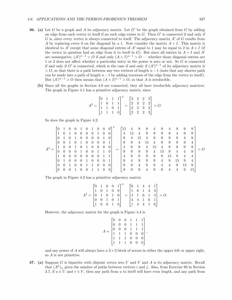
4.6. APPLICATIONS AND THE PERRON-FROBENIUS THEOREM 337
36. (a) Let G be a graph and A its adjacency matrix. Let G′ be the graph obtained from G by addingan edge from each vertex to itself if no such edge exists in G. Then G′ is connected if and only ifG is, since every vertex is always connected to itself. The adjacency matrix A′ of G results fromA by replacing every 0 on the diagonal by a 1. Now consider the matrix A + I. This matrix isidentical to A′ except that some diagonal entries of A′ equal to 1 may be equal to 2 in A+ I (ifthe vertex in question had an edge from it to itself in G). But since all entries in A + I and A′
are nonnegative, (A′)n−1 > O if and only (A+ I)n−1 > O — whether those diagonal entries are1 or 2 does not affect whether a particular entry in the power is zero or not. So G is connectedif and only if G′ is connected, which is the case if and only if (A′)n−1 of its adjacency matrix is> O, so that there is a path between any two vertices of length n− 1 (note that any shorter pathcan be made into a path of length n− 1 by adding traverses of the edge from the vertex to itself).But (A′)n−1 > O then means that (A+ I)n−1 > O, so that A is irreducible.
(b) Since all the graphs in Section 4.0 are connected, they all have irreducible adjacency matrices.The graph in Figure 4.1 has a primitive adjacency matrix, since
A2 =
0 1 1 11 0 1 11 1 0 11 1 1 0
2
=
3 2 2 22 3 2 22 2 3 22 2 2 3
> O.
So does the graph in Figure 4.2:
A4 =
0 1 0 0 1 0 1 0 0 01 0 1 0 0 0 0 1 0 00 1 0 1 0 0 0 0 1 00 0 1 0 1 0 0 0 0 11 0 0 1 0 1 0 0 0 00 0 0 0 1 0 0 1 1 01 0 0 0 0 0 0 0 1 10 1 0 0 0 1 0 0 0 10 0 1 0 0 1 1 0 0 00 0 0 1 0 0 1 1 0 0
4
=
15 4 9 9 4 9 4 9 9 94 15 4 9 9 9 9 4 9 99 4 15 4 9 9 9 9 4 99 9 4 15 4 9 9 9 9 44 9 9 4 15 4 9 9 9 99 9 9 9 4 15 9 4 4 94 9 9 9 9 9 15 9 4 49 4 9 9 9 4 9 15 9 49 9 4 9 9 4 4 9 15 99 9 9 4 9 9 4 4 9 15
> O
The graph in Figure 4.3 has a primitive adjacency matrix:
A4 =
0 1 0 0 11 0 1 0 00 1 0 1 00 0 1 0 11 0 0 1 0
4
=
6 1 4 4 11 6 1 4 44 1 6 1 44 4 1 6 11 4 4 1 6
> O.
However, the adjacency matrix for the graph is Figure 4.4 is
A =
0 0 0 1 1 10 0 0 1 1 10 0 0 1 1 11 1 1 0 0 01 1 1 0 0 01 1 1 0 0 0
,
and any power of A will always have a 3×3 block of zeroes in either the upper left or upper right,so A is not primitive.
37. (a) Suppose G is bipartite with disjoint vertex sets U and V and A is its adjacency matrix. Recallthat (Ak)ij gives the number of paths between vertices i and j. Also, from Exercise 80 in Section3.7, if u ∈ U and v ∈ V , then any path from u to itself will have even length, and any path from

338 CHAPTER 4. EIGENVALUES AND EIGENVECTORS
u to v will have odd length, since in any path, each successive edge moves you from U to V andback. So odd powers of A will have zero entries along the diagonal, while even powers of A willhave zero entries in any cell corresponding to a vertex in U and a vertex in V . Since every powerof A has a zero entry, A is not primitive.
(b) Number the vertices so that v1, v2, . . . , vk are in U and vk+1, vk+2, . . . , vn are in V . Then theadjacency matrix of G is
A =
[O BBT O
].
Write the eigenvector v corresponding to λ as
[v1
v2
], where v1 is a k-element column vector and
v2 is an (n− k)-element column vector. Then
Av = λv ⇐⇒[Bv2 B
Tv1
]=
[λv1
λv2
],
so that Bv2 = λv1 and BTv1 = λv2. Then
−λ[
v1
−v2
]=
[−λv1
λv2
]=
[−Bv2
BTv1
]= A
[−v1
v2
].
This shows that −λ is an eigenvalue of A with corresponding eigenvector
[−v1
v2
].
38. (a) Since each vertex of G connects to k other vertices, we see that each column of the adjacencymatrix A of G sums to k. Thus A = kP , where P is a matrix each of whose columns sums to1. So P is a transition matrix, and by Theorem 4.30, 1 is an eigenvalue of P , so that k is aneigenvalue of kP = A.
(b) If A is primitive, then Ar > O for some r, and therefore P r > O as well. Therefore P is regular,so by Theorem 4.31, every other eigenvalue of P has absolute value strictly less than 1, so thatevery other eigenvalue of A = kP has absolute value strictly less than k.
39. This exercise is left to the reader after doing the exploration suggested in Section 4.0.
40. (a) Let A = [aij ]. Then cA = [caij ], so that
|cA| = [|caij |] = [|c| · |aij |] = |c| [|aij |] = |c| · |A| .
(b) Using the Triangle Inequality,
|A+B| = [|aij + bij |] ≤ [|aij |+ |bij |] = [|aij |] + [|bij |] = |A|+ |B| .
(c) Ax is the n× 1 matrix whose ith entry is
ai1x1 + ai2x2 + · · ·+ ainxn.
Thus the ith entry of |Ax| is
|(Ax)i| = |ai1x1 + ai2x2 + · · ·+ ainxn|≤ |ai1x1|+ |ai2x2|+ · · ·+ |ainxn|= |ai1| |x1|+ |ai2| |x2|+ · · ·+ |ain| |xn| .
But this is just the ith entry of |A| |x|.(d) The ij entry of |AB| is
|AB|ij = |ai1b1j + ai2b2j + · · ·+ ainbnj |≤ |ai1b1j |+ |ai2b2j |+ · · ·+ |ainbnj |= |ai1| |b1j |+ |ai2| |b2j |+ · · ·+ |ain| |bnj | ,
which is the ij entry of |A| |B|.

4.6. APPLICATIONS AND THE PERRON-FROBENIUS THEOREM 339
41. A matrix is reducible if, after permuting rows and columns according to the same permutation, it canbe written [
B CO D
],
where B and D are square and O is the zero matrix. If A is 2 × 2, then B, C, O, and D must all be1× 1 matrices (which are therefore just the entries of A). If A is in the above form after applying nopermutations, leaving A alone, then a21 = 0. If A is in this form after applying the only other possiblepermutation — exchanging the two rows and the two columns — then the resulting matrix is[
a22 a21
a12 a11
],
so that a12 = 0. This proves the result.
42. (a) If λ1 and v1 are the Perron eigenvalue and eigenvector respectively, then by Theorem 4.37, λ1 > 0and v1 > 0. By Exercise 22 in Section 4.3, λ1 − 1 is an eigenvalue, with eigenvector v1, forA− I, and therefore 1− λ1 is an eigenvalue for I − A, again with eigenvector v1. Since I − A isinvertible, Theorem 4.18 says that 1
1−λ1is an eigenvalue for (I−A)−1, again with eigenvector v1.
But (I −A)−1 ≥ 0 and v1 ≥ 0, so that
1
1− λ1v1 = (I −A)−1v1 ≥ 0.
It follows that 11−λ1
≥ 0 and thus λ1 < 1. Since we also have λ1 > 0, the result follows: 0 < λ1 < 1.
(b) Since 0 < λ1 < 1, v1 > λ1v1 = Av1.
43. x0 = 1, x1 = 2x0 = 2, x2 = 2x1 = 4, x3 = 2x2 = 8, x4 = 2x3 = 16, x5 = 2x4 = 32.
44. a1 = 128, a2 = a12 = 64, a3 = a2
2 = 32, a4 = a32 = 16, a5 = a4
2 = 8.
45. y0 = 0, y1 = 1, y2 = y1 − y0 = 1, y3 = y2 − y1 = 0, y4 = y3 − y2 = −1, y5 = y4 − y3 = −1.
46. b0 = 1, b1 = 1, b2 = 2b1 + b0 = 3, b3 = 2b2 + b1 = 7, b4 = 2b3 + b2 = 17, b5 = 2b4 + b3 = 41.
47. The recurrence is xn−3xn−1−4xn−2 = 0, so the characteristic equation is λ2−3λ−4 = (λ−4)(λ+1) = 0.Thus the system has eigenvalues −1 and 4, so xn = c1(−1)n + c2 · 4n, where c1 and c2 are constants.Using the initial conditions, we have
0 = x0 = c1(−1)0 + c2 · 40 = c1 + c2,
5 = x1 = c1(−1)1 + c2 · 41 = −c1 + 4c2.
Add the two equations to solve for c2, then substitute back in to get c1 = −1 and c2 = 1, so thatxn = −(−1)n + 4n = 4n + (−1)n−1.
48. The recurrence is xn−4xn−1+3xn−2 = 0, so the characteristic equation is λ2−4λ+3 = (λ−3)(λ−1) = 0.Thus the system has eigenvalues 1 and 3, so xn = c1 ·1n+ c2 ·3n, where c1 and c2 are constants. Usingthe initial conditions, we have
0 = x0 = c1 · 10 + c2 · 30 = c1 + c2,
1 = x1 = c1 · 11 + c2 · 31 = c1 + 3c2.
Subtract the two equations to solve for c2, then substitute back in to get c1 = − 12 and c2 = 1
2 , so thatxn = − 1
2 · 1n + 1
2 · 3n = 1
2 (3n − 1).
49. The recurrence is yn− 4yn−1 + 4yn−2 = 0, so the characteristic equation is λ2− 4λ+ 4 = (λ− 2)2 = 0.Thus the system has the double eigenvalue 2, so yn = c1 · 2n + c2 · n2n, where c1 and c2 are constants.Using the initial conditions, we have
1 = y1 = c1 · 21 + c2 · 1 · 21 = 2c1 + 2c2,
6 = y2 = c1 · 22 + c2 · 2 · 22 = 4c1 + 8c2.
Solving the system gives c1 = − 12 and c2 = 1, so that yn = − 1
2 · 2n + n · 2n = n2n − 2n−1.

340 CHAPTER 4. EIGENVALUES AND EIGENVECTORS
50. The recurrence is an−an−1+ 14an−2 = 0, so the characteristic equation is 1
4 (4λ2−4λ+1) = 14 (2λ−1)2 =
0. Thus the system has the double eigenvalue 12 = 2−1, so an = c1 · 2−n + c2 · n2−n, where c1 and c2
are constants. Using the initial conditions, we have
4 = a0 = c1 · 2−0 + c2 · 0 · 2−0 = c1,
1 = a1 = c1 · 2−1 + c2 · 1 · 2−1 =1
2c1 +
1
2c2.
Solving the system gives c1 = 4 and c2 = −2, so that an = 4 · 2−n − 2n · 2−n = 22−n − n21−n.
51. The recurrence is bn − 2bn−1 − 2bn−2 = 0, so the characteristic equation is λ2 − 2λ − 2 = 0. Usingthe quadratic formula, this equation has roots λ = 1 ±
√3, which are therefore the eigenvalues. So
bn = c1 · (1+√
3)n+ c2 · (1−√
3)n, where c1 and c2 are constants. Using the initial conditions, we have
0 = b0 = c1 · (1 +√
3)0 + c2 · (1−√
3)0 = c1 + c2,
1 = b1 = c1 · (1 +√
3)1 + c2 · (1−√
3)1 = c1 + c2 + (c1 − c2)√
3.
From the first equation, c1 + c2 = 0, so the second becomes 1 = (c1 − c2)√
3, so that c1 − c2 =√
33 .
Since c2 = −c1, we get c1 =√
36 and c2 = −
√3
6 , so that the recurrence is
bn =
√3
6(1 +
√3)n −
√3
6(1−
√3)n =
√3
6
((1 +
√3)n − (1−
√3)n).
52. The recurrence is yn − yn−1 + yn−2 = 0, so the characteristic equation is λ2 − λ + 1 = 0. Using thequadratic formula, this equation has roots λ = 1
2 (1 ±√
3 i), which are therefore the eigenvalues. So
yn = c1 ·(
12 (1 +
√3 i))n
+c2 ·(
12 (1−
√3 i))n
, where c1 and c2 are constants. Using the initial conditions,we have
0 = y0 = c1 ·(
1
2(1 +
√3 i)
)0
+ c2 ·(
1
2(1−
√3 i)
)0
= c1 + c2,
1 = y1 = c1 ·(
1
2(1 +
√3 i)
)1
+ c2 ·(
1
2(1−
√3 i)
)1
=1
2c1(1 +
√3 i) +
1
2c2(1−
√3 i).
From the first equation, c1 + c2 = 0, so the second becomes 2 = (c1− c2)√
3 i, so that c1− c2 = − 2√
33 i.
Since c2 = −c1, we get c1 = −√
33 i and c2 =
√3
6 , so that the recurrence is
yn = −√
3
3i
(1
2(1 +
√3 i)
)n+
√3
3i
(1
2(1−
√3 i)
)n.
53. Working with the matrix A from the Theorem, since it has distinct eigenvalues λ1 6= λ2, it can bediagonalized, so that there is some invertible P such that
P =
[e fg h
], P−1AP = D =
[λ1 00 λ2
].
First consider the case where one of the eigenvalues, say λ2, is zero. In this case the matrix must beof the form
A =
[a 01 0
],
so that the other eigenvalue is a. In this case, the recurrence relation is xn = axn−1 + 0xn−2 = axn−1,so if we are given xj and xj−1 as initial conditions, we have xn = an−jxj . So take c1 = xja
−j andc2 = 0; then xn = c1λ
n1 + c2λ
n2 as desired. Now suppose that neither eigenvalue is zero. Then
Ak = PDkP−1 =1
eh− fg
[e fg h
] [λk1 00 λk2
] [h −f−g e
]=
1
eh− fg
[ehλk1 − fgλk2 −efλk1 + efλk2ghλk1 − ghλk2 −fgλk1 + ehλk2
].

4.6. APPLICATIONS AND THE PERRON-FROBENIUS THEOREM 341
If we are given two terms of the sequence, say xj−1 and xj , then for any n we have
xn =
[xnxn−1
]= An−jxj
=1
eh− fg
[ehλn−j1 − fgλn−j2 −efλn−j1 + efλn−j2
ghλn−j1 − ghλn−j2 −fgλn−j1 + ehλn−j2
] [xjxj−1
]
=1
eh− fg
(ehλn−j1 − fgλn−j2
)xj +
(−efλn−j1 + efλn−j2
)xj−1(
ghλn−j1 − ghλn−j2
)xj +
(−fgλn−j1 + ehλn−j2
)xj−1
=
1
eh− fg
((ehxj − efxj−1)λ−j1
)λn1 +
((−fgxj + efxj−1)λ−j2
)λn2(
(ghxj − fgxj−1)λ−j1
)λn1 +
((−ghxj + ehxj−1)λ−j2
)λn2
.Looking at the first row, we see that for
c1 =ehxj − efxj−1
eh− fgλ−j1 , c2 =
−fgxj + efxj−1
eh− fgλ−j2 ,
c1 and c2 are independent of n, and we have xn = c1λn1 + c2λ
n2 , as required.
54. (a) First suppose that the eigenvalues are distinct, i.e., that λ1 6= λ2. Then Exercise 53 gives oneformula for c1 and c2 involving the diagonalizing matrix P . But since we now know that c1 and c2exist, we can derive a simpler formula. We know the solutions are of the form xn = c1λ
n1 + c2λ
n2 ,
valid for all n. Since x0 = r and x1 = s, we get the following linear system in c1 and c2:
λ01c1 + λ0
2c2 = r or c1 + c2 = r
λ11c1 + λ1
2c2 = s λ1c1 + λ2c2 = s.
Solving this system, for example by setting up the augmented matrix and row-reducing, gives aunique solution
c1 = r − s− λ1r
λ2 − λ1, c2 =
s− λ1r
λ2 − λ1.
So the system has a unique solution in terms of x0 = r, x1 = s, λ1, and λ2. Note that the systemhas a unique solution (and these expressions make sense) since λ1 6= λ2.
Next suppose that the eigenvalues are the same, say λ1 = λ2 = λ. Then the solutions are ofthe form xn = c1λ
n + c2nλn. Note that we must have λ 6= 0, since otherwise the characteristic
polynomial of the recurrence matrix is λ2, so the recurrence relation is xn = 0. With x0 = r andx1 = s, we get the following linear system in c1 and c2:
λ0c1 + 0 · λ0c2 = r or c1 = r
λ1c1 + 1 · λ1c2 = s λc1 + λc2 = s.
Thus c1 = r, and substituting into the second equation gives (since λ 6= 0) c2 = s−λrλ . So in this
case as well we can find the scalars c1 and c2 uniquely. Finally, note that 0 is an eigenvalue of therecurrence matrix only when b = 0 in the recurrence relation xn = axn−1 + bxn−2.
(b) From part (a), the general solution to the recurrence is
xn = c1λn1 + c2λ
n2 =
(r − s− λ1r
λ2 − λ1
)λn1 +
(s− λ1r
λ2 − λ1
)λn2 .
Substituting x0 = r = 0 and x1 = s = 1 gives
xn =
(0− 1− λ1 · 0
λ2 − λ1
)λn1 +
(1− λ1 · 0λ2 − λ1
)λn2 =
1
λ2 − λ1(−λn1 + λn2 ) =
1
λ1 − λ2(λn1 − λn2 ).

342 CHAPTER 4. EIGENVALUES AND EIGENVECTORS
55. (a) For n = 1, since f0 = 0 and f1 = f2 = 1, the equation holds:
A1 = A =
[1 11 0
]=
[f2 f1
f1 f0
].
Now assume that the equation is true for n = k, and consider Ak+1:
Ak+1 = AkA =
[fk+1 fkfk fk−1
] [1 11 0
]=
[fk+1 + fk fk+1
fk + fk−1 fk
]=
[fk+2 fk+1
fk+1 fk
]as desired.
(b) Since detA = −1, it follows that det(An) = (detA)n
= (−1)n. But from part (a),
det(An) = fn+2fn − f2n+1 = (−1)n.
(c) If we look at the 5×13 “rectangle” as being composed of two “triangles”, we see that in fact theyare not triangles: the “diagonal” of the “rectangle” is not straight because the 8 × 3 triangularpieces are not similar to the entire triangles, since 5
13 6=38 . So there is empty space along the
diagonal of the figure that adds up to the missing 1 square unit.
56. (a) t1 = 1 (the only way is using the 1 × 1 rectangle); t2 = 3 (two 1 × 1 rectangles or either of the1× 2 rectangles); t3 = 5; t4 = 11; t5 = 21. For t0, we can think of that as the number of ways totile an empty rectangle; there is only one way — using no rectangles.
(b) The rightmost rectangle in a tiling of a 1 × n rectangle is either the 1 × 1 or one of the 1 × 2rectangles. So the number of tilings of a 1× n rectangle is the number of tilings of a 1× (n− 1)rectangle (adding the 1 × 1) plus twice the number of tilings of a 1 × (n − 2) rectangle (addingeither 1× 2). So the recurrence relation is
tn = tn−1 + 2tn−2.
(c) The characteristic equation is λ2 − λ − 2 = (λ − 2)(λ + 1), so the eigenvalues are −1 and 2. Tofind the constants, we solve
t1 = 1 = c1(−1)1 + c2 · 21 = −c1 + 2c2
t2 = 3 = c1(−1)2 + c2 · 22 = c1 + 4c2.
This gives c1 = 13 and c2 = 2
3 , so that
tn =1
3(−1)n +
2
3· 2n =
1
3
((−1)n + 2n+1
).
Evaluating for various values of t gives
t0 =1
3
((−1)0 + 2
)= 1, t1 =
1
3
((−1)1 + 22
)= 1,
t2 =1
3
((−1)2 + 23
)= 3, t3 =
1
3
((−1)3 + 24
)= 5,
t4 =1
3
((−1)4 + 25
)= 11, t5 =
1
3
((−1)5 + 26
)= 21.
These agree with part (a).
57. (a) d1 = 1, d2 = 2, d3 = 3, d4 = 5, d5 = 8. As in Exercise 56, d0 can be interpreted as the number ofways to cover a 2× 0 rectangle, which is one — use no dominos.
(b) The right end of any tiling of a 2 × n rectangle either consists of a domino laid vertically, or oftwo dominos each laid horizontally. Removing those leaves either a 2 × (n − 1) or a 2 × (n − 2)rectangle. So the number of tilings of a 2 × n rectangle is equal to the number of tilings of a2× (n− 1) rectangle plus the number of tilings of a 2× (n− 2) rectangle, or
dn = dn−1 + dn−2.
4.6. APPLICATIONS AND THE PERRON-FROBENIUS THEOREM 343
(c) We recognize the recurrence as the recurrence for the Fibonacci sequence; the initial values shiftit by 1, so we get
dn =1√5
(1 +√
5
2
)n+1
− 1√5
(1−√
5
2
)n+1
.
Computing values using this formula gives the same values as in part (a), including the value ford0.
58. Row-reducing gives
[A− 1+
√5
2 I 0]
=
[1− 1+
√5
2 0
1 − 1+√
52
]→
[1 −1−
√5
2
0 0
][A− 1−
√5
2 I 0]
=
[1− 1−
√5
2 0
1 − 1−√
52
]→
[1 −1+
√5
2
0 0
].
So the eigenvectors are
v1 =
[1+√
52
1
]and v2 =
[1−√
52
1
].
Then
limk→∞
xkλk1
= limk→∞
1√5
(1+√
52
)k− 1√
5
(1−√
52
)k1√5
(1+√
52
)k−1
− 1√5
(1−√
52
)k−1
(
1+√
52
)k= limk→∞
1√5− 1√
5
(1−√
51+√
5
)k1√5· 2
1+√
5− 1√
5· 1−
√5
2
(1−√
51+√
5
)k .
Since∣∣∣ 1−√5
1+√
5
∣∣∣ ≈ 0.381 < 1, the terms involving kth powers of this fraction go to zero as k →∞, leaving
us with (in the limit)[1√5
2√5(1+
√5)
]=
2√5(1 +
√5)
[1+√
52
1
]=
2√5(1 +
√5)
v1 =5−√
5
10v1,
which is a constant times v1.
59. The coefficient matrix has characteristic polynomial[1− λ 3
2 2− λ
]= (1− λ)(2− λ)− 6 = λ2 − 3λ− 4 = (λ− 4)(λ+ 1),
so that the eigenvalues are λ1 = 4 and λ2 = −1. The corresponding eigenvectors are found by row-reduction: [
A− 4I 0]
=
[−3 3 0
2 −2 0
]→[1 −1 00 0 0
]⇒ v1 =
[11
][A+ I 0
]=
[2 3 02 3 0
]→[1 3
2 00 0 0
]⇒ v2 =
[3−2
].
Then by Theorem 4.40,
x = C1e4t
[11
]+ C2e
−t[
3−2
].

344 CHAPTER 4. EIGENVALUES AND EIGENVECTORS
Substitute t = 0 to determine the constants:
x(0) =
[05
]= C1e
0
[11
]+ C2e
0
[3−2
]=
[C1 + 3C2
C1 − 2C2
].
These two equations give C1 = 3 and C2 = −1, so that the solution is
x = 3e4t
[11
]− e−t
[3−2
], or
x(t) = 3e4t − 3e−t
y(t) = 3e4t + 2e−t.
60. The coefficient matrix has characteristic polynomial[2− λ −1−1 2− λ
]= (2− λ)2 − 1 = λ2 − 4λ+ 3 = (λ− 1)(λ− 3),
so that the eigenvalues are λ1 = 1 and λ2 = 3. The corresponding eigenvectors are found by row-reduction: [
A− I 0]
=
[1 −1 0−1 1 0
]→[1 −1 00 0 0
]⇒ v1 =
[11
][A− 3I 0
]=
[−1 −1 0−1 −1 0
]→[1 1 00 0 0
]⇒ v2 =
[1−1
].
Then by Theorem 4.40,
x = C1et
[11
]+ C2e
3t
[1−1
].
Substitute t = 0 to determine the constants:
x(0) =
[11
]= C1e
0
[11
]+ C2e
0
[1−1
]=
[C1 + C2
C1 − C2
].
These two equations give C1 = 1 and C2 = 0, so that the solution is
x = et[11
]+ 0 · e3t
[1−1
], or
x(t) = et
y(t) = et.
61. The coefficient matrix has characteristic polynomial[1− λ 1
1 −1− λ
]= (1− λ)(−1− λ)− 1 = λ2 − 2 = (λ−
√2 )(λ+
√2 ),
so that the eigenvalues are λ1 =√
2 and λ2 = −√
2. The corresponding eigenvectors are found byrow-reduction:[
A−√
2I 0]
=
[1−√
2 1 0
1 −1−√
2 0
]→[1 −1−
√2 0
0 0 0
]⇒ v1 =
[1 +√
21
][A+√
2I 0]
=
[1 +√
2 1 0
1 −1 +√
2 0
]→[1 −1 +
√2 0
0 0 0
]⇒ v2 =
[1−√
21
].
Then by Theorem 4.40,
x = C1e√
2 t
[1 +√
21
]+ C2e
−√
2 t
[1−√
21
].
Substitute t = 0 to determine the constants:
x(0) =
[10
]= C1e
0
[1 +√
21
]+ C2e
0
[1−√
21
]=
[C1(1 +
√2) + C2(1−
√2)
C1 + C2
].

4.6. APPLICATIONS AND THE PERRON-FROBENIUS THEOREM 345
The second equation gives C1 +C2 = 0; substituting into the first equation gives (C1 −C2)√
2 = 1, so
that C1 − C2 =√
22 . It follows that C1 =
√2
4 and C2 = −√
24 , so that the solution is
x =
√2
4e√
2 t
[1 +√
21
]−√
2
4e−√
2 t
[1−√
21
], or
x1(t) =2 +√
2
4e√
2 t +2−√
2
4e−√
2 t
x2(t) =
√2
4
(e√
2 t − e−√
2 t).
62. The coefficient matrix has characteristic polynomial[1− λ −1
1 1− λ
]= (1− λ)2 + 1 = λ2 − 2λ+ 2,
so that the eigenvalues are λ1 = 1 + i and λ2 = 1 − i. The corresponding eigenvectors are found byrow-reduction: [
A− (1 + i)I 0]
=
[−i −1 0
1 −i 0
]→[1 −i 00 0 0
]⇒ v1 =
[i1
][A− (1− i)I 0
]=
[i −1 01 i 0
]→[1 i 00 0 0
]⇒ v2 =
[−i1
].
Then by Theorem 4.40,
y = C1e(1+i)t
[i1
]+ C2e
(1−i)t[−i1
].
Substitute t = 0 to determine the constants:
y(0) =
[11
]= C1e
0
[i1
]+ C2e
0
[−i1
]=
[(C1 − C2)iC1 + C2
].
Solving gives C1 = 1−i2 , C1 = 1+i
2 , so that the solution is
y =1− i
2e(1+i)t
[i1
]+
1 + i
2e(1−i)t
[−i1
],
or
y1(t) =1− i
2e(1+i)ti+
1 + i
2e(1−i)t · (−i) =
i+ 1
2e(1+i)t +
1− i2
e(1−i)t
y2(t) =1− i
2e(1+i)t +
1 + i
2e(1−i)t.
Now substitute cos t+ i sin t for eit, giving
y1(t) =i+ 1
2e(1+i)t +
1− i2
e(1−i)t
=i+ 1
2et(cos t+ i sin t) +
1− i2
et(cos t− i sin t)
= et cos t+
(i− 1
2+−i− 1
2
)et sin t
= et(cos t− sin t)
y2(t) =1− i
2e(1+i)t +
1 + i
2e(1−i)t
=1− i
2et(cos t+ i sin t) +
1 + i
2et(cos t− i sin t)
= et cos t+
(1 + i
2+
1− i2
)et sin t
= et(cos t+ sin t).

346 CHAPTER 4. EIGENVALUES AND EIGENVECTORS
63. The coefficient matrix has characteristic polynomial−λ 1 −11 −λ 11 1 −λ
= −λ3 + λ = −λ(1− λ)(1 + λ),
so that the eigenvalues are λ1 = 0, λ2 = 1, and λ3 = −1. The corresponding eigenvectors are found byrow-reduction:
[A− 0I 0
]=
0 1 −1 01 0 1 01 1 0 0
→1 0 1 0
0 1 −1 00 0 0 0
⇒ v1 =
−111
[A− I 0
]=
−1 1 −1 01 −1 1 01 1 −1 0
→1 0 0 0
0 1 −1 00 0 0 0
⇒ v2 =
011
[A+ I 0
]=
1 1 −1 01 1 1 01 1 1 0
→1 1 0 0
0 0 1 00 0 0 0
⇒ v2 =
−110
.Then by Theorem 4.40,
x = C1e0t
−111
+ C2et
011
+ C3e−t
−110
.Substitute t = 0 to determine the constants:
x(0) =
10−1
= C1e0
−111
+ C2e0
011
+ C3e0
−110
=
−C1 − C3
C1 + C2 + C3
C1 + C2
Solving gives C1 = −2, C3 = 1, C2 = 1, so that the solution is
x = −2
−111
+ et
011
+ e−t
−110
or
x(t) = 2− e−t
y(t) = −2 + et + e−t
z(t) = −2 + et.
64. The coefficient matrix has characteristic polynomial1− λ 0 31 −2− λ 13 0 −λ
= −(λ− 4)(λ+ 2)2
so that the eigenvalues are λ1 = 4 and λ2 = −2 (with algebraic multiplicity 2). The correspondingeigenvectors are found by row-reduction:
[A− 4I 0
]=
−3 0 3 01 −6 1 03 0 −3 0
→1 0 −1 0
0 1 − 13 0
0 0 0 0
⇒ v1 =
313
[A+ 2I 0
]=
3 0 3 01 0 1 03 0 3 0
→1 0 1 0
0 0 0 00 0 0 0
⇒ v2 =
010
,v3 =
−101
.

4.6. APPLICATIONS AND THE PERRON-FROBENIUS THEOREM 347
Then by Theorem 4.40,
x = C1e4t
313
+ C2e−2t
010
+ C3e−2t
−101
.Substitute t = 0 to determine the constants:
x(0) =
234
= C1e0
313
+ C2e0
010
+ C3e0
−101
=
3C1 − C3
C1 + C2
3C1 + C3
Solving gives C1 = 1, C2 = 2, C3 = 1, so that the solution is
x = e4t
313
+ 2e−2t
010
+ e−2t
−101
or
x(t) = 3e4t − e−2t
y(t) = e4t + 2e−2t
z(t) = 3e4t + e−2t.
65. (a) The coefficient matrix has characteristic polynomial[1.2− λ −0.2−0.2 1.5− λ
]= (1.2− λ)(1.5− λ)− 0.04 = λ2 − 2.7λ+ 1.76 = (λ− 1.1)(λ− 1.6)
so that the eigenvalues are λ1 = 1.1 and λ2 = 1.6. The corresponding eigenvectors are found byrow-reduction:[
A− 1.1I 0]
=
[0.1 −0.2 00.2 0.4 0
]→[1 −2 00 0 0
]⇒ v1 =
[21
][A− 1.6I 0
]=
[−0.4 −0.2 0−0.2 −0.1 0
]→[1 1
2 00 0 0
]⇒ v2 =
[−1
2
].
Then by Theorem 4.40,
x = C1e1.1t
[21
]+ C2e
1.6t
[−1
2
].
Substitute t = 0 to determine the constants:
x(0) =
[400500
]= C1e
0
[21
]+ C2e
0
[−1
2
]=
[2C1 − C2
C1 + 2C2
].
Solving gives C1 = 260, C2 = 120, so that the solution is
x = 260e1.1t
[21
]+ 120e1.6t
[−1
2
]or
x(t) = 520e1.1t − 120e1.6t
y(t) = 260e1.1t + 240e1.6t.
A plot of the populations over time is

348 CHAPTER 4. EIGENVALUES AND EIGENVECTORS
X
Y
0.5 1.0 1.5 2.0 2.5 3.0Time HdaysL0
5000
10 000
15 000
Population
From the graph, the population of Y dies out after about three days.
(b) Substituting a and b for 400 and 500 in the initial value computation above gives
x(0) =
[ab
]= C1e
0
[21
]+ C2e
0
[−1
2
]=
[2C1 − C2
C1 + 2C2
].
Solving gives C1 = 15 (2a+ b), C2 = 1
5 (−a+ 2b), so that the solution is
x =1
5(2a+ b)e1.1t
[21
]+
1
5(−a+ 2b)e1.6t
[−1
2
]or
x(t) =2
5(2a+ b)e1.1t − 1
5(−a+ 2b)e1.6t
y(t) =1
5(2a+ b)e1.1t +
2
5(−a+ 2b)e1.6t.
In the long run, the e1.6t term will dominate, so if a > 2b, then −a + 2b < 0, so the coefficientof e1.6t in x(t) is positive and in y(t) is negative, so that Y will die out and X will dominate.If a < 2b, then −a + 2b > 0, so the reverse will happen — X will die out and Y will dominate.Finally, if a = 2b, then the e1.6t term disappears in the solutions, and both populations will growat a rate proportional to e1.1t, though one will grow twice as fast as the other.
66. The coefficient matrix has characteristic polynomial[−0.8− λ 0.4
0.4 −0.2− λ
]= (−0.8− λ)(−0.2− λ)− 0.16 = λ2 + λ = λ(λ+ 1)
so that the eigenvalues are λ1 = 0 and λ2 = −1. The corresponding eigenvectors are found by row-reduction: [
A− 0I 0]
=
[−0.8 0.4 0
0.4 −0.2 0
]→[1 − 1
2 00 0 0
]⇒ v1 =
[12
][A+ I 0
]=
[0.2 0.4 00.4 0.8 0
]→[1 2 00 0 0
]⇒ v2 =
[−2
1
].
Then by Theorem 4.40,
x = C1e0t
[12
]+ C2e
−t[−2
1
].
Substitute t = 0 to determine the constants:
x(0) =
[1510
]= C1e
0
[12
]+ C2e
0
[−2
1
]=
[C1 − 2C2
2C1 + C2
].
Solving gives C1 = 7, C2 = −4, so that the solution is
x = 7
[12
]− 4e−t
[−2
1
]or
x(t) = 7 + 8e−t
y(t) = 14− 4e−t.
As t→∞, the exponential terms go to zero, and the populations stabilize at 7 of X and 14 of Y .

4.6. APPLICATIONS AND THE PERRON-FROBENIUS THEOREM 349
67. We want to convert x′ = Ax + b into an equation u′ = Au. If we could write b = Ab′, then lettingu = x + b′ would do the trick. To find b′, we invert A:
b′ = A−1b =
[12 − 1
212
12
][−30
−10
]=
[−10
−20
].
Then let u = x +
[−10−20
], so that
u′ =
(x +
[−10−20
])′= x′ = Ax + b = Ax +AA−1
[−10−20
]= A
(x +A−1
[−10−20
])= Au.
So now we want to solve this equation. A has characteristic polynomial[1− λ 1−1 1− λ
]= (1− λ)2 + 1 = λ2 − 2λ+ 2,
so the eigenvalues are 1 + i and 1− i. Eigenvectors are found by row-reducing:[A− (1 + i)I 0
]=
[−i 1 0−1 −i 0
]→[1 i 00 0 0
]⇒ v1 =
[1i
][A− (1− i)I 0
]=
[i 1 0−1 i 0
]→[1 −i 00 0 0
]⇒ v2 =
[i1
].
Then by Theorem 4.40,
u = C1e(1+i)t
[1i
]+ C2e
(1−i)t[i1
].
Substitute t = 0 to determine the constants:
u(0) = x(0) +
[−10−20
]=
[1010
]= C1e
0
[1i
]+ C2e
0
[i1
]=
[C1 + iC2
iC1 + C2
].
Solving gives C1 = C2 = 5− 5i, so that the solution is
u = (5− 5i)e(1+i)t
[1i
]+ (5− 5i)e(1−i)t
[i1
]= (5− 5i)et(cos t+ i sin t)
[1i
]+ (5− 5i)et(cos t− i sin t)
[i1
]= et
[(5− 5i) cos t+ (5 + 5i) sin t+ (5 + 5i) cos t+ (5− 5i) sin t
(5 + 5i) cos t+ (−5 + 5i) sin t+ (5− 5i) cos t+ (−5− 5i) sin t
]= et
[10 cos t+ 10 sin t10 cos t− 10 sin t
].
Rewriting in terms of the original variables gives
x = et[10 cos t+ 10 sin t10 cos t− 10 sin t
]−[−10−20
]= et
[10 cos t+ 10 sin t10 cos t− 10 sin t
]+
[1020
].
A plot of the populations is below. Both populations die out; species Y after about 1.2 time units andspecies X after about 2.4.
X
Y
0.0 0.5 1.0 1.5 2.0 2.5 3.0Time HdaysL0
10
20
30
40
50
60
Population

350 CHAPTER 4. EIGENVALUES AND EIGENVECTORS
68. We want to convert x′ = Ax + b into an equation u′ = Au. If we could write b = Ab′, then lettingu = x + b′ would do the trick. To find b′, we invert A:
b′ = A−1b =
[− 1
2 − 12
12 − 1
2
][0
40
]=
[−20
−20
].
Then let u = x +
[−20−20
], so that
u′ =
(x +
[−20−20
])′= x′ = Ax + b = Ax +AA−1
[0
40
]= A
(x +A−1
[0
40
])= Au.
So now we want to solve this equation. A has characteristic polynomial[−1− λ 1−1 −1− λ
]= (−1− λ)2 + 1 = λ2 + 2λ+ 2,
so the eigenvalues are −1 + i and −1− i. Eigenvectors are found by row-reducing:[A− (−1 + i)I 0
]=
[−i 1 0−1 −i 0
]→[1 i 00 0 0
]⇒ v1 =
[1i
][A− (−1− i)I 0
]=
[i 1 0−1 i 0
]→[1 −i 00 0 0
]⇒ v2 =
[i1
].
Then by Theorem 4.40,
u = C1e(−1+i)t
[1i
]+ C2e
(−1−i)t[i1
].
Substitute t = 0 to determine the constants:
u(0) = x(0) +
[−20−20
]=
[−10
10
]= C1e
0
[1i
]+ C2e
0
[i1
]=
[C1 + iC2
iC1 + C2
].
Solving gives C1 = −5− 5i and C2 = 5 + 5i, so that the solution is
u = (−5− 5i)e(−1+i)t
[1i
]+ (5 + 5i)e(−1−i)t
[i1
]= (−5− 5i)e−t(cos t+ i sin t)
[1i
]+ (5 + 5i)e−t(cos t− i sin t)
[i1
]= e−t
[(−5− 5i) cos t+ (5− 5i) sin t+ (−5 + 5i) cos t+ (5 + 5i) sin t
(5− 5i) cos t+ (5 + 5i) sin t+ (5 + 5i) cos t+ (5− 5i) sin t
]= e−t
[−10 cos t+ 10 sin t10 cos t+ 10 sin t
].
Rewriting in terms of the original variables gives
x = e−t[−10 cos t+ 10 sin t10 cos t+ 10 sin t
]−[−20−20
]= e−t
[−10 cos t+ 10 sin t10 cos t+ 10 sin t
]+
[2020
].
A plot of the populations is below; both populations stabilize at 20 as the e−t term goes to zero.
X
Y
0 1 2 3 4 5Time HdaysL0
5
10
15
20
25
30
Population

4.6. APPLICATIONS AND THE PERRON-FROBENIUS THEOREM 351
69. (a) Making the change of variables y = x′ and z = x, the original equation x′′+ax′+ bx = 0 becomesy′ + ay + bz = 0; since z = x, we have z′ = x′ = y. So we get the system
y′ = −ay − bzz′ = y .
(b) The coefficient matrix of the system in (a) is[−a −b
1 0
],
whose characteristic polynomial is (−a− λ)(−λ) + b = λ2 + aλ+ b.
70. Make the substitutions y1 = x(n−1), y2 = x(n−2), . . . , yn−1 = x′, yn = x. Then the original equation
x(n) + an−1x(n−1) + · · ·+ a1x
′ + a0 = 0
can be written as
y′1 + an−1y1 + an−2y2 + · · ·+ a2yn−2 + a1yn−1 + a0yn = 0,
and for i = 2, 3, . . . , n, we have y′i = yi−1. So we get the n equations
y′1 = an−1y1 − an−2y2 − · · · − a2yn−2 − a1yn−1 − a0yn
y′2 = y1
y′3 = y2
...
y′n = yn−1
whose coefficient matrix is −an−1 −an−2 · · · −a1 −a0
1 0 · · · 0 00 1 · · · 0 0...
.... . .
......
0 0 · · · 1 0
.This is the companion matrix of p(λ).
71. From Exercise 69, we know that the characteristic polynomial is λ2 − 5λ+ 6, so the eigenvalues are 2and 3. Therefore the general solution is x(t) = C1e
2t + C2e3t.
72. From Exercise 69, we know that the characteristic polynomial is λ2 + 4λ+ 3, so the eigenvalues are −1and −3. Therefore the general solution is x(t) = C1e
−t + C2e−3t.
73. From Exercise 59, the matrix of the system has eigenvalues 4 and −1 with corresponding eigenvectors[11
]and
[3−2
]. So by Theorem 4.41, the system x′ = Ax has solution x = eAtx(0). In this case
x(0) =
[05
], we get
eAT = P (et)DP−1 =
[1 3
1 −2
][e4t 0
0 e−t
][1 3
1 −2
]−1
=
[25e
4t + 35e−t 3
5e4t − 3
5e−t
25e
4t − 25e−t 3
5e4t + 2
5e−t
].
Thus the solution is [25e
4t + 35e−t 3
5e4t − 3
5e−t
25e
4t − 25e−t 3
5e4t + 2
5e−t
][0
5
]=
[3e4t − 3e−t
3e4t + 2e−t
],
which matches the result from Exercise 59.

352 CHAPTER 4. EIGENVALUES AND EIGENVECTORS
74. From Exercise 60, the matrix of the system has eigenvalues 1 and 3 with corresponding eigenvectors[11
]and
[1−1
]. So by Theorem 4.41, the system x′ = Ax has solution x = eAtx(0). In this case
x(0) =
[11
], we get
eAT = P (et)DP−1 =
[1 1
1 −1
][et 0
0 e3t
][1 1
1 −1
]−1
=
[12et + 1
2e3t 1
2et − 1
2e3t
12et − 1
2e3t 1
2et + 1
2e3t
].
Thus the solution is [12et + 1
2e3t 1
2et − 1
2e3t
12et − 1
2e3t 1
2et + 1
2e3t
][1
1
]=
[et
et
],
which matches the result from Exercise 60.
75. From Exercise 63, the matrix of the system has eigenvalues 0, 1, and−1 with corresponding eigenvectors−111
,
011
, and
−110
. So by Theorem 4.41, the system x′ = Ax has solution x = eAtx(0). In this
case x(0) =
10−1
, and we get
eAT = P (et)DP−1 =
−1 0 −11 1 11 1 0
1 0 00 et 00 0 e−t
−1 0 −11 1 11 1 0
−1
=
1 1− e−t −1 + e−t
−1 + e−t −1 + e−t + et 1− e−t−1 + et −1 + et 1
.Thus the solution is 1 1− e−t −1 + e−t
−1 + e−t −1 + e−t + et 1− e−t−1 + et −1 + et 1
10−1
=
2− e−t−2 + et + e−t
−2 + et
,which matches the result from Exercise 63.
76. From Exercise 64, the matrix of the system has eigenvalues 4 and −2 (with algebraic multiplicity 2)
with corresponding eigenvectors
313
and
0
10
,−1
01
. So by Theorem 4.41, the system x′ = Ax
has solution x = eAtx(0). In this case x(0) =
234
, and we get
eAT = P (et)DP−1 =
3 0 −1
1 1 0
3 0 1
e4t 0 0
0 e−2t 0
0 0 e−2t
3 0 −1
1 1 0
3 0 1
−1
=
12e
4t + 12e−2t 0 1
2e4t − 1
2e−2t
16e
4t − 16e−2t e−2t 1
6e4t − 1
6e−2t
12e
4t − 12e−2t 0 1
2e4t + 1
2e−2t
.

4.6. APPLICATIONS AND THE PERRON-FROBENIUS THEOREM 353
Thus the solution is 12e
4t + 12e−2t 0 1
2e4t − 1
2e−2t
16e
4t − 16e−2t e−2t 1
6e4t − 1
6e−2t
12e
4t − 12e−2t 0 1
2e4t + 1
2e−2t
2
3
4
=
3e4t − e−2t
e4t + 2e−2t
3e4t + e−2t
,which matches the result from Exercise 64.
77. (a) With A =
[2 10 3
], we have
x1 = A
[11
]=
[33
], x2 = Ax1 =
[99
], x3 = Ax2 =
[2727
].
5 10 15 20 25
5
10
15
20
25
(b) With A =
[2 10 3
], we have
x1 = A
[10
]=
[20
], x2 = Ax1 =
[40
], x3 = Ax2 =
[80
].
2 4 6 8
-1.0
-0.5
0.5
1.0
(c) Since the matrix is upper triangular, we see that its eigenvalues are 2 and 3; since these are bothgreater than 1 in magnitude, the origin is a repeller.
(d) Some other trajectories are
-5 5 10
-10
-5
5
10

354 CHAPTER 4. EIGENVALUES AND EIGENVECTORS
78. (a) With A =
[0.5 −0.5
0 0.5
], we have
x1 = A
[11
]=
[0
0.5
], x2 = Ax1 =
[−0.250.25
], x3 = Ax2 =
[−0.250.125
].
-0.2 0.2 0.4 0.6 0.8 1.0
0.2
0.4
0.6
0.8
1.0
(b) With A =
[0.5 −0.5
0 0.5
], we have
x1 = A
[10
]=
[0.50
], x2 = Ax1 =
[0.25
0
], x3 = Ax2 =
[0.125
0
].
0.2 0.4 0.6 0.8 1.0 1.2 1.4
-0.1
0.1
(c) Since the matrix is upper triangular, we see that its only eigenvalue is 0.5; since this is less than1 in magnitude, the origin is an attractor.
(d) Some other trajectories are
-1.0 -0.5 0.5 1.0 1.5 2.0
-2.0
-1.5
-1.0
-0.5
0.5
1.0
79. (a) With A =
[2 −1−1 2
], we have
x1 = A
[11
]=
[11
],
so that
[11
]is a fixed point:

4.6. APPLICATIONS AND THE PERRON-FROBENIUS THEOREM 355
0.5 1.0 1.5 2.0
0.5
1.0
1.5
2.0
(b) With A =
[2 −1−1 2
], we have
x1 = A
[10
]=
[2−1
], x2 = Ax1 =
[5−4
], x3 = Ax2 =
[14−13
].
2 4 6 8 10 12 14
-12
-10
-8
-6
-4
-2
(c) The characteristic polynomial of the matrix is
det(A− λI) =
[2− λ −1−1 2− λ
]= λ2 − 4λ+ 3 = (λ− 3)(λ− 1).
Thus one eigenvalue is greater than 1 in magnitude and the other is equal to 1. So the origin isnot a repeller, an attractor, or a saddle point; there are no nonzero values of x0 for which thetrajectory of x0 approaches the origin.
(d) Some other trajectories are
-5 5 10
-10
-5
5
10
80. (a) With A =
[−4 2
1 −3
], we have
x1 = A
[11
]=
[−2−2
], x2 = Ax1 =
[44
], x3 = Ax2 =
[−8−8
].
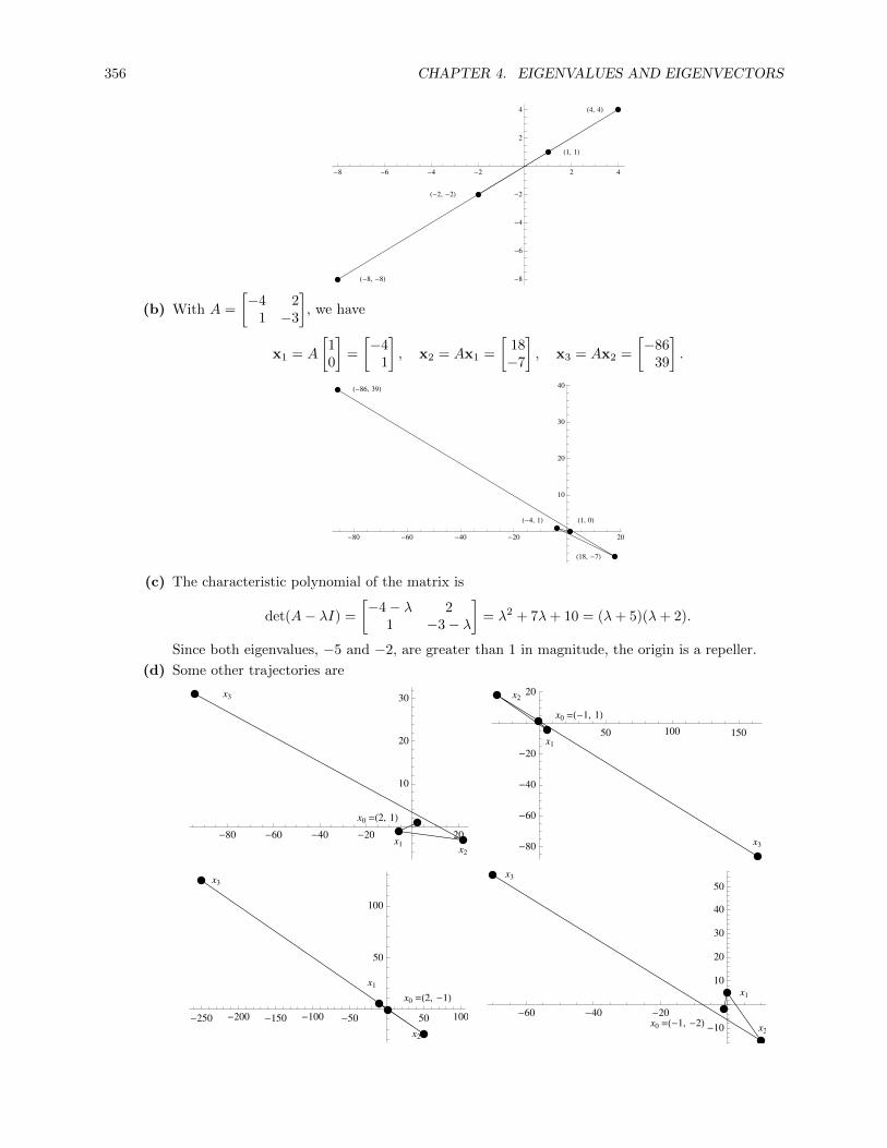
356 CHAPTER 4. EIGENVALUES AND EIGENVECTORS
H1, 1L
H-2, -2L
H4, 4L
H-8, -8L
-8 -6 -4 -2 2 4
-8
-6
-4
-2
2
4
(b) With A =
[−4 2
1 −3
], we have
x1 = A
[10
]=
[−4
1
], x2 = Ax1 =
[18−7
], x3 = Ax2 =
[−86
39
].
H1, 0LH-4, 1L
H18, -7L
H-86, 39L
-80 -60 -40 -20 20
10
20
30
40
(c) The characteristic polynomial of the matrix is
det(A− λI) =
[−4− λ 2
1 −3− λ
]= λ2 + 7λ+ 10 = (λ+ 5)(λ+ 2).
Since both eigenvalues, −5 and −2, are greater than 1 in magnitude, the origin is a repeller.
(d) Some other trajectories are
x0 =H2, 1L
x1x2
x3
-80 -60 -40 -20 20
10
20
30
x0 =H-1, 1L
x1
x2
x3
50 100 150
-80
-60
-40
-20
20
x0 =H2, -1L
x1
x2
x3
-250 -200 -150 -100 -50 50 100
50
100
x0 =H-1, -2L
x1
x2
x3
-60 -40 -20
-10
10
20
30
40
50

4.6. APPLICATIONS AND THE PERRON-FROBENIUS THEOREM 357
81. (a) With A =
[1.5 −1−1 0
], we have
x1 = A
[11
]=
[−2−2
], x2 = Ax1 =
[44
], x3 = Ax2 =
[−8−8
].
H1, 1L
H0.5, -1L
H1.75, -0.5L
H3.125, -1.75L
0.5 1.0 1.5 2.0 2.5 3.0
-1.5
-1.0
-0.5
0.5
1.0
(b) With A =
[1.5 −1−1 0
], we have
x1 = A
[10
]=
[−4
1
], x2 = Ax1 =
[18−7
], x3 = Ax2 =
[−86
39
].
H1, 0L
H1.5, -1L
H3.25, -1.5L
H6.375, -3.25L
1 2 3 4 5 6
-3.0
-2.5
-2.0
-1.5
-1.0
-0.5
(c) The characteristic polynomial of the matrix is
det(A− λI) =
[1.5− λ −1−1 −λ
]= λ2 − 1.5λ+ 1 = (λ− 2)(λ+ 0.5)
Since one eigenvalue is greater than 1 in magnitude and the other is less, the origin is a saddlepoint. Eigenvectors for λ = −0.5 are attracted to the origin, and other vectors are repelled.

358 CHAPTER 4. EIGENVALUES AND EIGENVECTORS
(d) Some other trajectories are
x0 =H1, 2L
x1
x2
x3
-0.4 -0.2 0.2 0.4 0.6 0.8 1.0
-1.0
-0.5
0.5
1.0
1.5
2.0
x0 =H-1, 1L
x1
x2
x3
-8 -6 -4 -2
1
2
3
4
5
x0 =H2, -1L
x1
x2
x3
5 10 15
-8
-6
-4
-2
x0 =H-1, -2L
x1
x2
x3
-1.0 -0.8 -0.6 -0.4 -0.2 0.2 0.4
-2.0
-1.5
-1.0
-0.5
0.5
1.0
82. (a) With A =
[0.1 0.90.5 0.5
], we have
x1 = A
[11
]=
[11
],
so
[11
]is a fixed point - it is an eigenvector for the eigenvalue λ = 1.
H1, 1L
0.5 1.0 1.5 2.0
0.5
1.0
1.5
2.0
(b) With A =
[0.1 0.90.5 0.5
], we have
x1 = A
[10
]=
[0.10.5
], x2 = Ax1 =
[0.460.30
], x3 = Ax2 =
[0.3160.38
].

4.6. APPLICATIONS AND THE PERRON-FROBENIUS THEOREM 359
H1, 0L
H0.1, 0.5L
H0.46, 0.3L
H0.316, 0.38L
0.2 0.4 0.6 0.8 1.0
0.1
0.2
0.3
0.4
0.5
(c) The characteristic polynomial of the matrix is
det(A− λI) =
[0.1− λ 0.9
0.5 0.5− λ
]= λ2 − 0.6λ− 0.45 = (λ− 1)(λ+ 0.4).
Since one eigenvalue is less than 1 in magnitude and the other is equal to 1, the origin is neitheran attractor, a repeller, nor a saddle point.
(d) Some other trajectories are
x0 =H2, 1L
x1
x2
x3
0.0 0.5 1.0 1.5 2.0
0.5
1.0
1.5 x0 =H-9, 5L
x1
x2
x3
-8 -6 -4 -2 2
-2
-1
1
2
3
4
5
x0 =H-1, -2L
x1
x2
x3
-2.0 -1.5 -1.0 -0.5
-2.0
-1.5
-1.0
-0.5
x0 =H1, -1L
x1
x2
x3
-0.5 0.5 1.0
-1.0
-0.8
-0.6
-0.4
-0.2
83. (a) With A =
[0.2 0.4−0.2 0.8
], we have
x1 = A
[11
]=
[0.60.6
], x2 = Ax1 =
[0.360.36
], x2 = Ax2 =
[0.2160.216
].

360 CHAPTER 4. EIGENVALUES AND EIGENVECTORS
0.4 0.6 0.8 1.0
0.4
0.6
0.8
1.0
(b) With A =
[0.2 0.4−0.2 0.8
], we have
x1 = A
[10
]=
[0.2−0.2
], x2 = Ax1 =
[−0.04−0.20
], x3 = Ax2 =
[−0.088−0.152
].
-0.2 0.2 0.4 0.6 0.8 1.0
-0.3
-0.2
-0.1
0.1
0.2
(c) The characteristic polynomial of the matrix is
det(A− λI) =
[0.2− λ 0.4−0.2 0.8− λ
]= λ2 − λ+ 0.24 = (λ− 0.4)(λ− 0.6).
Since both eigenvalues are smaller than 1 in magnitude, the origin is an attractor.
(d) Some other trajectories are
-2 -1 1 2
-4
-2
2
4
84. (a) With A =
[0 −1.5
1.2 3.6
], we have
x1 = A
[11
]=
[−1.5
4.8
], x2 = Ax1 =
[−7.215.48
], x2 = Ax2 =
[−23.2247.088
].

4.6. APPLICATIONS AND THE PERRON-FROBENIUS THEOREM 361
-20 -15 -10 -5
10
20
30
40
(b) With A =
[0 −1.5
1.2 3.6
], we have
x1 = A
[10
]=
[0
1.2
], x2 = Ax1 =
[−1.84.32
], x3 = Ax2 =
[−6.4813.392
].
-6 -5 -4 -3 -2 -1 1
2
4
6
8
10
12
(c) The characteristic polynomial of the matrix is
det(A− λI) =
[−λ −1.51.2 3.6− λ
]= λ2 − 3.6λ+ 1.8 = (λ− 3)(λ− 0.6).
Since one eigenvalue is smaller than 1 in magnitude and the other is greater, the origin is a saddlepoint; the origin attracts some initial points and repels others.
(d) Some other trajectories are
-4 -2 2 4
-4
-2
2
4
6
85. With the given matrix A, we have r =√a2 + b2 =
√2 and θ = π
4 , so that
A =
[r 0
0 r
][cos θ − sin θ
sin θ cos θ
]=
[√2 0
0√
2
][1√2− 1√
21√2
1√2
].
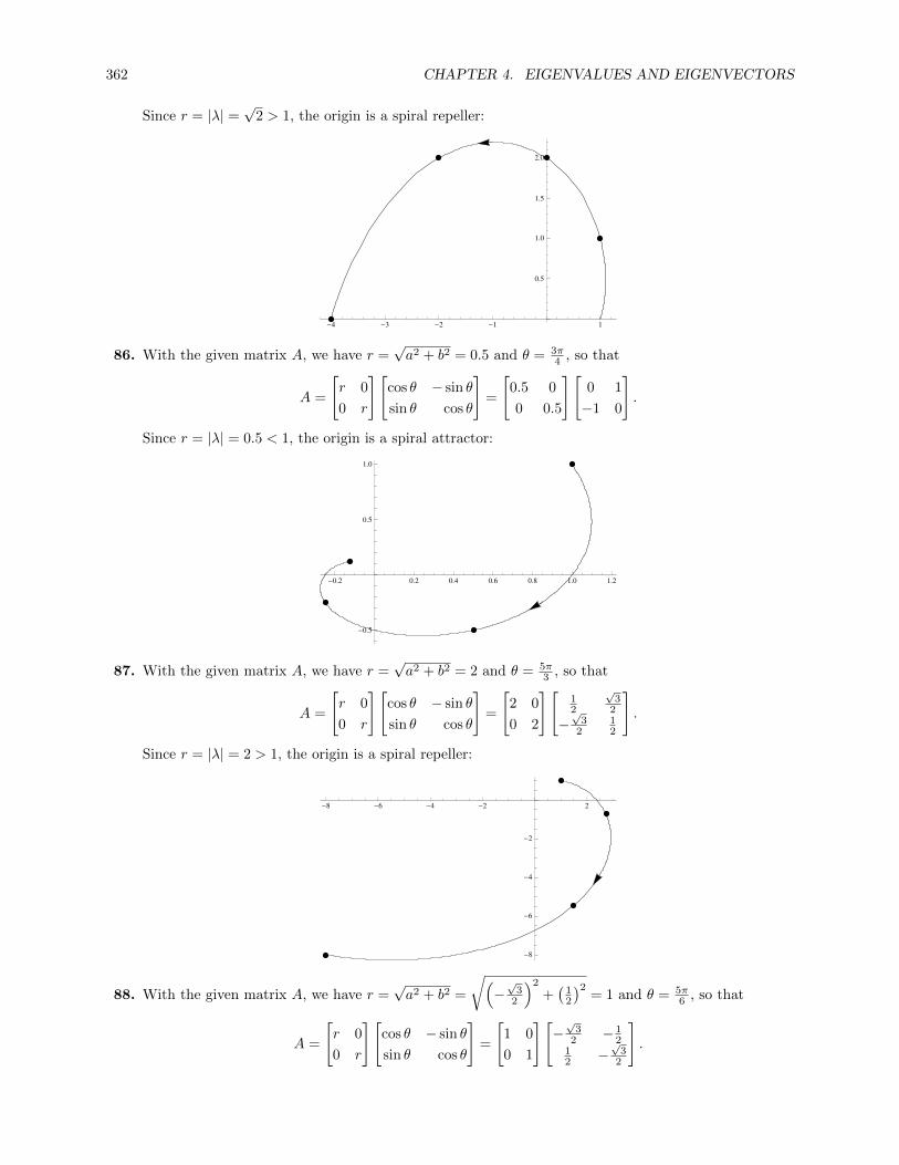
362 CHAPTER 4. EIGENVALUES AND EIGENVECTORS
Since r = |λ| =√
2 > 1, the origin is a spiral repeller:
-4 -3 -2 -1 1
0.5
1.0
1.5
2.0
86. With the given matrix A, we have r =√a2 + b2 = 0.5 and θ = 3π
4 , so that
A =
[r 0
0 r
][cos θ − sin θ
sin θ cos θ
]=
[0.5 0
0 0.5
][0 1
−1 0
].
Since r = |λ| = 0.5 < 1, the origin is a spiral attractor:
-0.2 0.2 0.4 0.6 0.8 1.0 1.2
-0.5
0.5
1.0
87. With the given matrix A, we have r =√a2 + b2 = 2 and θ = 5π
3 , so that
A =
[r 0
0 r
][cos θ − sin θ
sin θ cos θ
]=
[2 0
0 2
][12
√3
2
−√
32
12
].
Since r = |λ| = 2 > 1, the origin is a spiral repeller:
-8 -6 -4 -2 2
-8
-6
-4
-2
88. With the given matrix A, we have r =√a2 + b2 =
√(−√
32
)2
+(
12
)2= 1 and θ = 5π
6 , so that
A =
[r 0
0 r
][cos θ − sin θ
sin θ cos θ
]=
[1 0
0 1
][−√
32 − 1
212 −
√3
2
].

4.6. APPLICATIONS AND THE PERRON-FROBENIUS THEOREM 363
Since r = |λ| = 1, the origin is the orbital center:
x0
x1 x2
x3
-1.0 -0.5 0.5 1.0
-1.0
-0.5
0.5
1.0
89. The characteristic polynomial of A is
det(A− λI) =
[0.1− λ −0.2
0.1 0.3− λ
]= λ2 − 0.4λ+ 0.05;
solving this quadratic gives λ = 0.2 ± 0.1i for the eigenvalues. Row-reducing gives
[−1− i
1
]for an
eigenvector. Thus P =[Rex Imx
]=
[−1 −1
1 0
], and so
C = P−1AP =
[0 1−1 −1
] [0.1 −0.20.1 0.3
] [−1 −1
1 0
]=
[0.2 −0.10.1 0.2
].
Since |λ| =√
0.05 < 1, the origin is a spiral attractor. The first six points are
x0 =
[11
], x1 =
[−0.1
0.4
], x2 =
[−0.09
0.11
],
x3 =
[−0.031
0.024
], x4 =
[−0.0079
0.0041
], x5 =
[−0.00161
0.00044
].
0.2 0.4 0.6 0.8 1.0
0.2
0.4
0.6
0.8
1.0
90. The characteristic polynomial of A is
det(A− λI) =
[2− λ 1−2 −λ
]= λ2 − 2λ+ 2;

364 CHAPTER 4. EIGENVALUES AND EIGENVECTORS
solving this quadratic gives λ = 1 ± i for the eigenvalues. Row-reducing gives
[−1− i
2
]for an eigen-
vector. Thus P =[Rex Imx
]=
[−1 −1
2 0
], and so
C = P−1AP =
[0 1
2
−1 − 12
][2 1
−2 0
][−1 −1
2 0
]=
[1 1
−1 1
].
Since |λ| =√
2 > 1, the origin is a spiral repeller. The first six points are
x0 =
[11
], x1 =
[3−2
], x2 =
[4−6
], x3 =
[2−8
], x4 =
[−4−4
], x5 =
[−12
8
].
-10 -5
-5
5
91. The characteristic polynomial of A is
det(A− λI) =
[1− λ −1
1 −λ
]= λ2 − λ+ 1;
solving this quadratic gives λ = 12 ±
√3
2 i for the eigenvalues. Row-reducing gives
[12 −
√3
2 i1
]for an
eigenvector. Thus
P =[Rex Imx
]=
[12 −
√3
21 0
],
and so
C = P−1AP =
[0 1
− 2√3
1√3
][1 −1
1 0
][12 −
√3
2
1 0
]=
[12 −
√3
2√3
212
].
Since |λ| = 1, the origin is an orbital center. The first six points are
x0 =
[11
], x1 =
[01
], x2 =
[−1
0
], x3 =
[−1−1
], x4 =
[0−1
], x5 =
[10
].
-1.0 -0.5 0.5 1.0
-1.0
-0.5
0.5
1.0

Chapter Review 365
92. The characteristic polynomial of A is
det(A− λI) =
[−λ −1
1√
3− λ
]= λ2 −
√3λ+ 1;
solving this quadratic gives λ =√
32 ±
12 i for the eigenvalues. Row-reducing gives
[−√
32 −
12 i
1
]for an
eigenvector. Thus
P =[Rex Imx
]=
[−√
32 − 1
21 0
],
and so
C = P−1AP =
[0 1
−2 −√
3
][0 −1
1√
3
][−√
32 − 1
2
1 0
]=
[√3
2 − 12
12
√3
2
].
Since |λ| = 1, the origin is an orbital center. The first six points are
x0 =
[11
], x1 =
[−1
1 +√
3
], x2 =
[−1−
√3
2 +√
3
],
x3 =
[−2−
√3
2 +√
3
], x4 =
[−2−
√3
1 +√
3
], x5 =
[−1−
√3
1
].
-3 -2 -1 1 2 3
-3
-2
-1
1
2
3
Chapter Review
1. (a) False. What is true is that if A is an n× n matrix, then det(−A) = (−1)n detA. This is becausemultiplying any row by −1 multiplies the determinant by −1, and −A multiplies every row by−1. See Theorem 4.7.
(b) True, since det(AB) = det(A) det(B) = det(B) det(A) = det(BA). See Theorem 4.8.
(c) False. It depends on what order the columns are in. Swapping any two columns of A multipliesthe determinant by −1. See Theorem 4.4.
(d) False. While detAT = detA by Theorem 4.10, detA−1 = 1detA by Theorem 4.9. So unless
detA = ±1, the statement is false.
(e) False. For example, the matrix
[0 10 0
]has a characteristic polynomial of 0, so 0 is its only
eigenvalue.
(f) False. For example, the identity matrix has only λ = 1 as an eigenvalue, but ei is an eigenvectorfor every i.
(g) True. See Theorem 4.25 in Section 4.4.
(h) False. Any diagonal matrix with two identical entries on the diagonal (such as the identity matrix)provides a counterexample.

366 CHAPTER 4. EIGENVALUES AND EIGENVECTORS
(i) False. If A and B are similar, then they have the same eigenvalues, but not necessarily the sameeigenvectors. Exercise 48 in Section 4.4 shows that if B = P−1AP and v is an eigenvector of A,then P−1v is an eigenvector for B for the same eigenvalue.
(j) False. For example, if A is invertible, then its reduced row echelon form is the identity matrix,which has only the eigenvalue 1. So if A has an eigenvalue other than 1, it cannot be similar tothe identity matrix.
2. (a) For example, expand along the first row:∣∣∣∣∣∣1 3 53 5 77 9 11
∣∣∣∣∣∣ = 1
∣∣∣∣5 79 11
∣∣∣∣− 3
∣∣∣∣3 77 11
∣∣∣∣+ 5
∣∣∣∣3 57 9
∣∣∣∣= 1(5 · 11− 7 · 9)− 3(3 · 11− 7 · 7) + 5(3 · 9− 5 · 7)
= 0.
(b) Apply row operations to diagonalize the matrix:1 3 53 5 77 9 11
R2−3R1−−−−−→R3−7R1−−−−−→
1 3 50 −4 −80 −12 −24
R3−3R2−−−−−→
1 3 50 −4 −80 0 0
.Then detA is the product of the diagonal entries, which is zero.
3. To get from the first matrix to the second:
• Multiply the first column by 3; this multiplies the determinant by 3.
• Multiply the second column by 2; this multiplies the determinant by 2.
• Subtract 4 times the third column from the second; this does not change the determinant.
• Interchange the first and second rows; this multiplies the determinant by −1.
So the determinant of the resulting matrix is 3 · 3 · 2 · (−1) = −18.
4. (a) We have
detC = det((AB)−1
)=
1
det(AB)=
1
detAdetB=
1
2 ·(− 1
4
) = −2.
(b) We have
detC = det(A2B(3AT )
)= detA · detA · detB · det(3AT )
= −det(3AT ) = −34 det(AT ) = −34 detA = −162.
5. For any n× n matrix, detA = det(AT ), and det(−A) = (−1)n detA. So if A is skew-symmetric, thenAT = −A and
detA = det(AT ) = det(−A) = (−1)n detA = −detA
since n is odd. But detA = −detA means that detA = 0.
6. Compute the determinant by expanding along the first row:∣∣∣∣∣∣1 −1 21 1 k2 4 k2
∣∣∣∣∣∣ = 1
∣∣∣∣1 k4 k2
∣∣∣∣− (−1)
∣∣∣∣1 k2 k2
∣∣∣∣+ 2
∣∣∣∣1 12 4
∣∣∣∣= 1(k2 − 4k) + 1(k2 − 2k) + 2(4− 2)
= 2k2 − 6k + 4 = 2(k − 2)(k − 1).
So the determinant is zero when k = 1 or k = 2.

Chapter Review 367
7. Since
Ax =
[3 14 3
] [12
]=
[510
]= 5
[12
],
we see that x is indeed an eigenvector, with corresponding eigenvalue 5.
8. Since
Ax =
13 −60 −45−5 18 1510 −40 −32
3−1
2
=
3 · 13− 1 · (−60) + 2 · (−45)3 · (−5)− 1 · 18 + 2 · 15
3 · 10− 1 · (−40) + 2 · (−32)
=
9−3
6
= 3
3−1
2
,we see that x is indeed an eigenvector, with corresponding eigenvalue 3.
9. (a) The characteristic polynomial of A is
det(A− λI) =
∣∣∣∣∣∣−5− λ −6 3
3 4− λ −30 0 −2− λ
∣∣∣∣∣∣= (−2− λ)
∣∣∣∣−5− λ −63 4− λ
∣∣∣∣= −(λ+ 2)(λ2 + λ− 2) = −(λ+ 2)(λ+ 2)(λ− 1).
(b) The eigenvalues of A are the roots of the characteristic polynomial, which are λ1 = 1 and λ2 = −2(with algebraic multiplicity 2).
(c) We row-reduce A− λI for each eigenvalue λ:
[A− I 0
]=
−6 −6 3 03 3 −3 00 0 −3 0
R1↔R2−−−−−→
3 3 −3 0−6 −6 3 0
0 0 −3 0
13R1−−−→
− 13R3−−−−→
1 1 −1 0−6 −6 3 0
0 0 1 0
R2+6R1−−−−−→
1 1 −1 00 0 −3 00 0 1 0
R2↔R3−−−−−→
1 1 −1 00 0 1 00 0 −3 0
R1+R2−−−−−→
R3+3R1−−−−−→
1 1 0 00 0 1 00 0 0 0
[A+ 2I 0
]=
−3 −6 3 03 6 −3 00 0 0 0
R2+R2−−−−−→
−3 −6 3 00 0 0 00 0 0 0
− 13R1−−−−→
1 2 −1 00 0 0 00 0 0 0
.Thus the eigenspaces are
E1 = span
−110
, E−2 =
−2s+ t
st
= span
−210
,1
01
.
(d) Even though A does not have three distinct eigenvalues, it is diagonalizable since the eigenvalueof algebraic multiplicity 2, which is λ2 = −2, also has geometric multiplicity 2. A diagonalizingmatrix is a matrix P whose columns are the eigenvectors above, so
P =
−1 −2 11 1 00 0 1
,

368 CHAPTER 4. EIGENVALUES AND EIGENVECTORS
and
P−1AP =
1 2 −1−1 −1 1
0 0 1
−5 −6 33 4 −30 0 −2
−1 −2 11 1 00 0 1
=
1 0 00 −2 00 0 −2
= D.
10. Since A is diagonalizable, A ∼ D where D is a diagonal matrix whose diagonal entries are its eigen-values. Since A ∼ D, we know that A and D have the same eigenvalues, so the diagonal entries ofD are −2, 3, and 4 and thus detD = −24. But A ∼ D also implies that detD = det(P−1AP ) =det(P−1) detA detP = detA, so that detA = −24.
11. Since [37
]= 5
[11
]− 2
[1−1
],
we know by Theorem 4.19 that
A−5
[37
]= 5
(1
2
)−5 [11
]− 2(−1)−5
[1−1
]=
[160160
]+
[2−2
]=
[162158
].
12. Since A is diagonalizable, it has n linearly independent eigenvectors, which therefore form a basis forRn. So if x is any vector, then x =
∑civi for some constants ci, so that by Theorem 4.19, and using
the Triangle Inequality,
‖Anx‖ =
∥∥∥∥∥An(
n∑i=1
civi
)∥∥∥∥∥ =∥∥∥∑ ciλ
ni vi
∥∥∥ ≤∑ |ci| |λi|n ‖vi‖ .
Then |λi|n → 0 as n→∞ since |λi| < 1, so each term of this sum goes to zero, so that ‖Anx‖ → 0 asn→∞. Since this holds for all vectors x, it follows that An → O as n→∞.
13. The two characteristic polynomials are
pA =
∣∣∣∣4− λ 23 1− λ
∣∣∣∣ = (4− λ)(1− λ)− 6 = λ2 − 5λ− 2
pB =
∣∣∣∣2− λ 23 2− λ
∣∣∣∣ = (2− λ)(2− λ)− 6 = λ2 − 4λ− 2.
Since the characteristic polynomials are different, the matrices are not similar.
14. Since both matrices are diagonal, we can read off their eigenvalues; both matrices have eigenvalues 2and 3. To convert A to B, we want to reverse the rows, and reverse the columns, so choose
P = P−1 =
[0 11 0
].
Then
P−1AP =
[0 11 0
] [2 00 3
] [0 11 0
]=
[3 00 2
]= B.
15. These matrices are not similar. If there were, then there would be some 3× 3 matrix
P =
a b cd e fg h i
such that P−1AP = B, or AP = PB. But
AP =
a+ d b+ e c+ fd+ g e+ h f + ig h i
PB =
a a+ b cd d+ e fg g + h i
.
Chapter Review 369
If these matrices are to be equal, then comparing entries in the last row and column gives f = i = g = 0.The upper left entries also give d = 0. The two middle entries are e+h and d+ e = e, so that h = 0 aswell. Thus the entire bottom row of P is zero, so P cannot be invertible and A and B are not similar.Note that this is a counterexample to the converse of Theorem 4.22. These two matrices satisfy parts(a) through (g) of the conclusion, yet they are not similar.
16. The characteristic polynomial of A is
det(A− λI) =
∣∣∣∣2− λ k1 −λ
∣∣∣∣ = (2− λ)(−λ)− k = λ2 − 2λ− k.
(a) A has eigenvalues 3 and −1 if λ2 − 2λ− k = (λ− 3)(λ+ 1), so when k = 3.
(b) A has an eigenvalue with algebraic multiplicity 2 when its characteristic polynomial has a doubleroot, which occurs when its discriminant is 0. But its discriminant is (−2)2− 4 · 1 · (−k) = 4 + 4k,so we must have k = −1.
(c) A has no real eigenvalues when the discriminant 4+4k of its characteristic polynomial is negative,so for k < −1.
17. If λ is an eigenvalue of A with eigenvector x, then Ax = λx, so that
A3x = A(A(A(x))) = A(A(λx)) = A(λ2x) = λ3x.
If A3 = A, then Ax = λ3x, so that λ = λ3 and then λ = 0 or λ = ±1.
18. If A has two identical rows, then Theorem 4.3(c) says that detA = 0, so that A is not invertible. Butthen by Theorem 4.17, 0 must be an eigenvalue of A.
19. If x is an eigenvalue of A with eigenvalue 3, then
(A2 − 5A+ 2I)x = A2x− 5Ax + 2Ix = 9x− 5 · 3x + 2x = −4x.
This shows that x is also an eigenvector of A2 − 5A+ 2I, with eigenvalue −4.
20. Suppose that B = P−1AP where P is invertible. This can be rewritten as BP−1 = P−1A. Let λ bean eigenvalue of A with eigenvector x. Then
B(P−1x) = (BP−1)x = (P−1A)x = P−1(Ax) = P−1(λx) = λ(P−1x).
Thus P−1x is an eigenvector for B, corresponding to λ.

Chapter 5
Orthogonality
5.1 Orthogonality in Rn
1. Since
v1 · v2 = (−3) · 2 + 1 · 4 + 2 · 1 = 0,
v1 · v3 = (−3) · 1 + 1 · (−1) + 2 · 2 = 0,
v2 · v3 = 2 · 1 + 4 · (−1) + 1 · 2 = 0,
this set of vectors is orthogonal.
2. Since
v1 · v2 = 4 · (−1) + 2 · 2− 5 · 0 = 0,
v1 · v3 = 4 · 2 + 2 · 1− 5 · 2 = 0,
v2 · v3 = −1 · 2 + 2 · 1 + 0 · 2 = 0,
this set of vectors is orthogonal.
3. Since v1 · v2 = 3 · (−1) + 1 · 2− 1 · 1 = −2 6= 0, this set of vectors is not orthogonal. There is no needto check the other two dot products; all three must be zero for the set to be orthogonal.
4. Since v1 · v3 = 5 · 3 + 3 · 1 + 1 · (−1) = 17 6= 0, this set of vectors is not orthogonal. There is no needto check the other two dot products; all three must be zero for the set to be orthogonal.
5. Since
v1 · v2 = 2 · (−2) + 3 · 1− 1 · (−1) + 4 · 0 = 0,
v1 · v3 = 2 · (−4) + 3 · (−6)− 1 · 2 + 4 · 7 = 0,
v2 · v3 = −2 · (−4) + 1 · (−6)− 1 · 2 + 0 · 7 = 0,
this set of vectors is orthogonal.
6. Since v2 · v4 = −1 · 0 + 0 · (−1) + 1 · 1 + 2 · 1 = 3 6= 0, this set of vectors is not orthogonal. There is noneed to check the other five dot products (they are all zero); all dot products must be zero for the setto be orthogonal.
7. Since the vectors are orthogonal: [4−2
]·[12
]= 4 · 1− 2 · 2 = 0,
371

372 CHAPTER 5. ORTHOGONALITY
they are linearly independent by Theorem 5.1. Since there are two vectors, they form an orthogonalbasis for R2. By Theorem 5.2, we have
w =v1 ·wv1 · v1
v1 +v2 ·wv2 · v2
v2 =4 · 1− 2 · (−3)
4 · 4− 2 · (−2)v1 +
1 · 1 + 2 · (−3)
1 · 1 + 2 · 2v2 =
1
2v1 − v2,
so that
[w]B =
[12−1
].
8. Since the vectors are orthogonal: [13
]·[−6
2
]= 1 · (−6) + 3 · 2 = 0,
they are linearly independent by Theorem 5.1. Since there are two vectors, they form an orthogonalbasis for R2. By Theorem 5.2, we have
w =v1 ·wv1 · v1
v1 +v2 ·wv2 · v2
v2 =1 · 1 + 3 · 11 · 1 + 3 · 3
v1 +−6 · 1 + 2 · 1−6 · (−6) + 2 · 2
v2 =2
5v1 −
1
10v2,
so that
[w]B =
[25
− 110
].
9. Since the vectors are orthogonal: 10−1
·1
21
= 1 · 1 + 0 · 2− 1 · 1 = 0
10−1
· 1−1
1
= 1 · 1 + 0 · (−1)− 1 · 1 = 0
121
· 1−1
1
= 1 · 1 + 2 · (−1) + 1 · 1 = 0,
they are linearly independent by Theorem 5.1. Since there are three vectors, they form an orthogonalbasis for R3. By Theorem 5.2, we have
w =v1 ·wv1 · v1
v1 +v2 ·wv2 · v2
v2 +v3 ·wv3 · v3
v3
=1 · 1 + 0 · 1− 1 · 1
1 · 1 + 0 · 0− 1 · (−1)v1 +
1 · 1 + 2 · 1 + 1 · 11 · 1 + 2 · 2 + 1 · 1
v2 +1 · 1− 1 · 1 + 1 · 1
1 · 1− 1 · (−1) + 1 · 1v3
=2
3v2 +
1
3v3,
so that
[w]B =
02313
.
5.1. ORTHOGONALITY IN RN 373
10. Since the vectors are orthogonal:111
· 1−1
0
= 1 · 1 + 1 · (−1) + 1 · 0 = 0
111
· 1
1−2
= 1 · 1 + 1 · 1 + 1 · (−2) = 0
1−1
0
· 1
1−2
= 1 · 1− 1 · 1 + 0 · (−2) = 0,
they are linearly independent by Theorem 5.1. Since there are three vectors, they form an orthogonalbasis for R3. By Theorem 5.2, we have
w =v1 ·wv1 · v1
v1 +v2 ·wv2 · v2
v2 +v3 ·wv3 · v3
v3
=1 · 1 + 1 · 2 + 1 · 31 · 1 + 1 · 1 + 1 · 1
v1 +1 · 1− 1 · 2 + 0 · 3
1 · 1− 1 · (−1) + 0 · 0v2 +
1 · 1 + 1 · 2− 2 · 31 · 1 + 1 · 1− 2 · (−2)
v3
= 2v1 −1
2v2 −
1
2v3,
so that
[w]B =
2
− 12
− 12
.11. Since ‖v1‖ =
√(35
)2+(
45
)2= 1 and ‖v2‖ =
√(− 4
5
)2+(
35
)2= 1, the given set of vectors is orthonor-
mal.
12. Since ‖v1‖ =
√(12
)2+(
12
)2= 1√
26= 1 and ‖v2‖ =
√(12
)2+(− 1
2
)2= 1√
26= 1, the given set of vectors
is not orthonormal. To normalize the vectors, we divide each by its norm to get{1
1/√
2
[1212
],
1
1/√
2
[12
− 12
]}=
{[1√2
1√2
],
[1√2
− 1√2
]}.
13. Taking norms, we get
‖v1‖ =
√(1
3
)2
+
(2
3
)2
+
(2
3
)2
= 1
‖v2‖ =
√(2
3
)2
+
(−1
3
)2
+ 02 =
√5
3
‖v3‖ =
√12 + 22 +
(5
2
)2
=3√
5
2.
So the first vector is already normalized; we must normalize the other two by dividing by their norms,to get
132323
, 1√5/3
23
− 13
0
, 1
3√
5/2
1
2
− 52
=
132323
,
2√5
− 1√5
0
,
23√
54
3√
5
− 53√
5
.

374 CHAPTER 5. ORTHOGONALITY
14. Taking norms, we get
‖v1‖ =
√(1
2
)2
+
(1
2
)2
+
(−1
2
)2
+
(1
2
)2
= 1
‖v2‖ =
√02 +
(1
3
)2
+
(2
3
)2
+
(1
3
)2
+ 02 =
√6
3
‖v3‖ =
√(1
2
)2
+
(−1
6
)2
+
(1
6
)2
+
(−1
6
)2
=
√3
3.
So the first vector is already normalized; we must normalize the other two by dividing by their norms,to get
1212
− 1212
, 1√6/3
0132313
, 1√3/3
12
− 1616
− 16
=
1212
− 1212
,
01√6
2√6
1√6
,√
32
−√
36√3
6
−√
36
.
15. Taking norms, we get
‖v1‖ =
√(1
2
)2
+
(1
2
)2
+
(−1
2
)2
+
(1
2
)2
= 1
‖v2‖ =
√√√√02 +
(√6
3
)2
+
(1√6
)2
+
(− 1√
6
)2
= 1
‖v3‖ =
√√√√(√3
2
)2
+
(−√
3
6
)2
+
(√3
6
)2
+
(−√
3
6
)2
= 1
‖v4‖ =
√02 + 02 +
(1√2
)2
+
(1√2
)2
= 1.
So these vectors are already orthonormal.
16. The columns of the matrix are orthogonal:[01
]·[−1
0
]= 0 · (−1) + 1 · 0 = 0.
Further, they are orthonormal since[01
]·[01
]= 0 · 0 + 1 · 1 = 1,
[−1
0
]·[−1
0
]= −1 · (−1) + 0 · 0 = 1.
Thus the matrix is an orthogonal matrix, so by Theorem 5.5, the inverse of this matrix is its transpose,or [
0 1−1 0
].
17. The columns of the matrix are orthogonal:[1√2
− 1√2
]·
[1√2
1√2
]=
1√2· 1√
2− 1√
2· 1√
2= 0.

5.1. ORTHOGONALITY IN RN 375
Further, they are orthonormal since[1√2
− 1√2
]·
[1√2
− 1√2
]=
1√2· 1√
2− 1√
2·(− 1√
2
)= 1
[1√2
1√2
]·
[1√2
1√2
]=
1√2· 1√
2+
1√2· 1√
2= 1.
Thus the matrix is an orthogonal matrix, so by Theorem 5.5, the inverse of this matrix is its transpose,or [
1√2− 1√
21√2
1√2
].
18. This is not an orthogonal matrix since none of the columns have norm 1:
q1 · q1 =1
9+
1
9+
1
9=
1
3, q2 · q2 =
1
4+
1
4+ 0 =
1
2, q3 · q3 =
1
25+
1
25+
4
25=
6
25.
19. This matrix Q is orthogonal by Theorem 5.4 since QQT = I:
QQT =
cos θ sin θ − cos θ − sin2 θcos2 θ sin θ − cos θ sin θsin θ 0 cos θ
cos θ sin θ cos2 θ sin θ− cos θ sin θ 0− sin2 θ − cos θ sin θ cos θ
=
cos2 θ sin2 θ+cos2 θ+sin4 θ cos3 θ sin θ−sin θ cos θ+cos θ sin3 θ cos θ sin2 θ−cos θ sin2 θ
cos3 θ sin θ−sin θ cos θ+cos θ sin3 θ cos4 θ+sin2 θ+cos2 θ sin2 θ cos2 θ sin θ−cos2 θ sin θ
sin2 θ cos θ−sin2 θ cos θ sin θ cos2 θ−cos2 θ sin θ sin2 θ+cos2 θ
=
1 0 00 1 00 0 1
.Thus by Theorem 5.5 Q−1 = QT .
20. The columns are all orthogonal since each dot product consists of two terms of 12 ·
12 and two of − 1
2 ·12 .
The columns are orthonormal since the norm of each column is√(±1
2
)2
+
(±1
2
)2
+
(±1
2
)2
+
(±1
2
)2
= 1.
So the matrix is orthonormal, so by Theorem 5.5 its inverse is equal to its transpose,12
12 − 1
212
− 12
12
12
12
12
12
12 − 1
212 − 1
212
12
.
21. The dot product of the first and fourth columns is1
0
0
0
·
1√6
1√6
− 1√6
1√2
= 1 · 1√66= 0,
so the matrix is not orthonormal.

376 CHAPTER 5. ORTHOGONALITY
22. By Theorem 5.5, Q−1 is orthogonal if and only if(Q−1
)T=(Q−1
)−1. But since Q is orthogonal,
Q−1 = QT , so that (Q−1
)T=(QT)−1
=(Q−1
)−1,
and Q−1 is orthogonal.
23. Since detQ = detQT , we have
1 = det(I) = det(QQ−1) = det(QQT ) = (detQ)(detQT ) = (detQ)2.
Since (detQ)2 = 1, we must have detQ = ±1.
24. By Theorem 5.5, it suffices to show that (Q1Q2)−1 = (Q1Q2)T . But using the fact that Q−11 = QT1
and Q−12 = QT2 , we have
(Q1Q2)−1 = Q−12 Q−1
1 = QT2 QT1 = (Q1Q2)T .
Thus Q1Q2 is orthogonal.
25. By Theorem 3.17, if P is a permutation matrix, then P−1 = PT . So by Theorem 5.5, P is orthogonal.
26. Reordering the rows of Q is the same as multiplying it on the left by a permutation matrix P . By theprevious exercise, P is orthogonal, and then by Exercise 24, PQ is also orthogonal. So reordering therows of an orthogonal matrix results in an orthogonal matrix.
27. Let θ be the angle between x and y, and φ the angle betweenQx andQy. By Theorem 5.6, ‖Qx‖ = ‖x‖,‖Qy‖ = ‖y‖, and Qx ·Qy = x · y, so that
cos θ =x · y‖x‖ ‖y‖
=Qx ·Qy
‖Qx‖ ‖Qy‖= cosφ.
Since 0 ≤ θ, φ ≤ π, the fact that their cosines are equal implies that θ = φ.
28. (a) Suppose that Q =
[a cb d
]is an orthogonal matrix. Then
QQT = QTQ = I ⇒[a bc d
] [a cb d
]=
[a2 + b2 ac+ bdac+ bd c2 + d2
]=
[1 00 1
].
So a2 + b2 = 1 and c2 + d2 = 1, and thus both columns of Q are unit vectors. Also, ac+ bd = 0,which implies that ac = −bd and therefore a2c2 = b2d2. But c2 = 1 − d2 and b2 = 1 − a2;substituting gives
a2(1− d2) = (1− a2)d2 ⇒ a2 − a2d2 = d2 − a2d2 ⇒ a2 = d2 ⇒ a = ±d.
If a = d = 0, then b = c = ±1, so we get one of the matrices[0 11 0
],
[0 −11 0
],
[0 1−1 0
],
[0 −1−1 0
],
all of which are of one of the required forms. Otherwise, if a = d 6= 0, then c2 = 1−d2 = 1−a2 = b2,so that b = ±c and we get [
a ±bb a
],
and we must choose the minus sign in order that the columns be orthogonal. So the result is[a −bb a
],

5.1. ORTHOGONALITY IN RN 377
which is also of the required form. Finally, if a = −d 6= 0, then again b2 = c2 and we get[a ±bb −a
];
this time we must choose the plus sign for the columns to be orthogonal, resulting in[a bb −a
],
which is again of the required form.
(b) Since
[ab
]is a unit vector, we have a2 +b2 = 1, so that (a, b) is a point on the unit circle. Therefore
there is some θ with (a, b) = (cos θ, sin θ). Substituting into the forms from part (a) gives thedesired matrices.
(c) Let
Q =
[cos θ − sin θsin θ cos θ
], R =
[cos θ sin θsin θ − cos θ
].
From Example 3.58 in Section 3.6, Q is the standard matrix of a rotation through angle θ. FromExercise 26(c) in Section 3.6, R is a reflection through the line ` that makes an angle of θ
2 with
the x-axis, which is the line y =(tan θ
2
)x (or x = 0 if θ = π).
(d) From part (c), we have detQ = cos2 θ + sin2 θ = 1 and detR = − cos2 θ − sin2 θ = −1.
29. Since detQ = 1√2· 1√
2−(− 1√
2· 1√
2
)= 1, this matrix represents a rotation. To find the angle, we have
cos θ = 1√2
and sin θ = 1√2, so that θ = π
4 = 45◦.
30. Since detQ = − 12 ·(− 1
2
)−√
32 ·
(−√
32
)= 1, this matrix represents a rotation. To find the angle, we
have cos θ = − 12 and sin θ = −
√3
2 , so that θ = 4π3 = 240◦.
31. Since detQ = − 12 ·(
12
)−√
32 ·
(√3
2
)= −1, this matrix represents a reflection. If cos θ = − 1
2 and
sin θ =√
32 , then θ = 2π
3 , so that by part (d) of the previous exercise the reflection occurs through the
line y =(tan π
3
)x =√
3x.
32. Since detQ = − 35 ·
35 −
(− 4
5
)·(− 4
5
)= −1, this matrix represents a reflection. Let θ be the (third
quadrant) angle with cos θ = − 35 and sin θ = − 4
5 ; then by part (d) of the previous exercise, the
reflection occurs through the line y =(tan θ
2
)x.
33. (a) Since A and B are orthogonal matrices, we know that AT = A−1 and BT = B−1, so that
A(AT +BT )B = A(A−1 +B−1
)B = AA−1B +AB−1B = B +A = A+B.
(b) Since A and B are orthogonal matrices, we have detA = ±1 and detB = ±1. If detA+detB = 0,then one of them must be 1 and the other must be −1, so that (detA)(detB) = −1. But by part(a),
det(A+B) = det(A(AT +BT )B
)= (detA)
(det(AT +BT )
)(detB)
= (detA)(det((A+B)T )
)(detB) = (detA)(detB) (det(A+B)) = −det(A+B).
Since det(A+B) = −det(A+B), we conclude that det(A+B) = 0 so that A+B is not invertible.
34. It suffices to show that QQT = I. Now,
QQT =
[x1 yT
y I −(
11−x1
)yyt
][x1 yT
y I −(
11−x1
)yyt
].

378 CHAPTER 5. ORTHOGONALITY
Also, x21 + yyT = x2
1 + x22 + · · · + x2
n = 1, since x is a unit vector. Rearranging gives yyT = 1 − x21.
Further, we have
yT(I −
(1
1− x1
)yyT
)= yT −
(1
1− x1
)yT (1− x1)2 = yT − (1 + x1)yT
= −x1yT(
I −(
1
1− x1
)yyT
)y = y −
(1
1− x1
)(1− x2
1)y = y − (1 + x1)y
= −x1y(I −
(1
1− x1
)yyT
)(I −
(1
1− x1
)yyT
)= I2 − 2
(1
1− x1
)yyT +
(1
1− x1
)2
yyTyyT
= I − 2(1− x1)
(1− x1)2yyT +
1− x21
(1− x1)2yyT
= I − 1− 2x1 + x21
(1− x1)2yyT
= I − yyT .
Then evaluating QQT gives
QQT =
x21 + yTy x1y
T + yT(I −
(1
1−x1
)yyT
)x1y +
(I −
(1
1−x1
)yyT
)y yyT +
(I −
(1
1−x1
)yyT
)(I −
(1
1−x1
)yyT
)=
[1 x1y
T − x1yT
x1y − x1y yyT + (I − yyT )
]=
[1 OO I
]= I.
Thus Q is orthogonal.
35. Let Q be orthogonal and upper triangular. Then the columns qi of Q are orthonormal; that is,
qi · qj =
n∑k=1
qkiqkj =
{0 i 6= j
1 i = j.
Since Q is upper triangular, we know that qij = 0 when i > j. We prove by induction on the rows thateach row has only one nonzero entry, along the diagonal. Note that q11 6= 0, since all other entries inthe first column are zero and the norm of the first column vector must be 1. Now the dot product ofq1 with qj for j > 1 is
q1 · qj =
n∑k=1
qk1qkj = q11q1j .
Since these columns must be orthogonal, this product is zero, so that q1j = 0 for j > 1 and thereforeq11 is the only nonzero entry in the first row. Now assume that q11, q22, . . . , qii are the only nonzeroentries in their rows, and consider qi+1,i+1. It is the only nonzero entry in its column, since entriesin lower-numbered rows are zero by the inductive hypothesis and entries in higher-numbered rows arezero since Q is upper triangular. Therefore, qi+1,i+1 6= 0 since the (i+ 1)st column must have norm 1.Now consider the dot product of qi+1 with qj for j > i+ 1:
qi+1 · qj =
n∑k=1
qk,i+1qkj = qi+1,i+1qi+1,j .

5.2. ORTHOGONAL COMPLEMENTS AND ORTHOGONAL PROJECTIONS 379
Since these columns must be orthogonal, this product is zero, so that qi+1,j = 0 for j > i + 1. So allentries to the right of the (i+ 1)st column are zero. But also entries to the left of the (i+ 1)st columnare zero since Q is upper triangular. Thus qi+1,i+1 is the only nonzero entry in its row. So inductively,qkk is the only nonzero entry in the kth row for k = 1, 2, . . . , n, so that Q is diagonal.
36. If n > m, then the maximum rank of A is m. By the Rank Theorem (Theorem 3.26, in Section 3.5),we know that rank(A) + nullity(A) = n; since n > m, we have nullity(A) = n −m > 0. So there issome nonzero vector x such that Ax = 0. But then ‖x‖ 6= 0 while ‖Ax‖ = ‖0‖ = 0.
37. (a) Since the {vi} are a basis, we may choose αi, βi such that
x =
n∑k=1
αkvk, y =
n∑k=1
βkvk.
Because {vi} form an orthonormal basis, we know that vi ·vi = 1 and vi ·vj = 0 for i 6= j. Then
x · y =
(n∑k=1
αkvk
)·
(n∑k=1
βkvk
)=
n∑i,j=1
αiβjvi · vj =
n∑i=1
αiβivi · vi =
n∑i=1
αiβi.
But x · vi =∑nk=1 αkvk · vi = αi and similarly y · vi = βi. Therefore the sum at the end of the
displayed equation above is
n∑i=1
αiβi =
n∑i=1
(x · vi)(y · vi) = (x · v1)(y · v1) + (x · v2)(y · v2) + · · ·+ (x · vn)(y · vn),
proving Parseval’s Identity.
(b) Since [x]B = [αk] and [y]B = [βk], Parseval’s Identity says that
x · y =
n∑k=1
αkβk = [x]B · [y]B.
In other words, the dot product is invariant under a change of orthonormal basis.
5.2 Orthogonal Complements and Orthogonal Projections
1. W is the column space of A =
[12
], so that W⊥ is the null space of AT =
[1 2
]. The augmented
matrix is already row-reduced: [1 2 0
],
so that a basis for the null space, and thus for W⊥, is given by[−2
1
].
2. W is the column space of A =
[−4
3
], so that W⊥ is the null space of AT =
[−4 3
]. Row-reducing
gives [−4 3 0
]→[1 − 3
4 0],
so that a basis for the null space, and thus for W⊥, is given by[34
1
], or
[3
4
].

380 CHAPTER 5. ORTHOGONALITY
3. W consists of xy
x+ y
= x
101
+ y
011
, so that
1
01
,0
11
is a basis for W.
Then W is the column space of
A =
1 00 11 1
,so that W⊥ is the null space of AT . The augmented matrix is already row-reduced:[
1 0 1 00 1 1 0
]so that the null space, which is W⊥, is the set−t−t
t
= t
−1−1
1
= span
−1−11
.
This vector forms a basis for W⊥.
4. W consists of x2x+ 3z
z
= x
120
+ y
031
, so that
1
20
,0
31
is a basis for W.
Then W is the column space of
A =
1 02 30 1
,so that W⊥ is the null space of AT . Row-reduce the augmented matrix:[
1 2 0 0
0 3 1 0
]→
[1 0 − 2
3 0
0 1 13 0
]so that the null space, which is W⊥, is the set
23 t
− 13 t
t
= t
23
− 13
1
= span
2
−1
3
.
This vector forms a basis for W⊥.
5. W is the column space of A =
1−1
3
, so that W⊥ is the null space of AT =[1 −1 3
]. The
augmented matrix is already row-reduced: [1 −1 3 0
],
so that the null space, which is W⊥, is the sets− 3tst
= s
110
+ t
−301
= span
110
,−3
01
These two vectors form a basis for W⊥.

5.2. ORTHOGONAL COMPLEMENTS AND ORTHOGONAL PROJECTIONS 381
6. W is the column space of A =
12
− 12
2
, so that W⊥ is the null space of AT =[
12 − 1
2 2]. Row-reducing
gives [12 − 1
2 2 0]→[1 −1 4 0
],
so the null space, which is W⊥, is the sets− 4tst
= s
110
+ t
−401
= span
110
,−4
01
These two vectors form a basis for W⊥.
7. To find the required bases, we row-reduce[A 0
]:
1 −1 3 05 2 1 00 1 −2 0−1 −1 1 0
→
1 0 1 00 1 −2 00 0 0 00 0 0 0
.Therefore, a basis for the row space of A is the nonzero rows of the reduced matrix, or
u1 =[1 0 1
], u2 =
[0 1 −2
].
The null space null(A) is the set of solutions of the augmented matrix, which are given by−s2ss
.Thus a basis for null(A) is
v =
−121
.Every vector in row(A) is orthogonal to every vector in null(A):
u1 · v = 1 · (−1) + 0 · 2 + 1 · 1 = 0, u2 · v = 0 · (−1) + 1 · 2− 2 · 1 = 0.
8. To find the required bases, we row-reduce[A 0
]:
1 1 −1 0 2 0−2 0 2 4 4 0
2 2 −2 0 1 0−3 −1 3 4 5 0
→
1 0 −1 −2 0 00 1 0 2 0 00 0 0 0 1 00 0 0 0 0 0
.Thus a basis for the row space of A is the nonzero rows of the reduced matrix, or
u1 =[1 0 −1 −2 0
], u2 =
[0 1 0 2 0
], u3 =
[0 0 0 0 1
].
The null space null(A) is the set of solutions of the augmented matrix, which are given bys+ 2t−2tst0
= s
10100
+ t
2−2
010
= span
10100
,
2−2
010
.

382 CHAPTER 5. ORTHOGONALITY
Thus a basis for null(A) is
v1 =
10100
, v2 =
2−2
010
.Every vector in row(A) is orthogonal to every vector in null(A):
u1 · v1 = 1 · 1 + 0 · 0− 1 · 1− 2 · 0 + 0 · 0 = 0, u1 · v2 = 1 · 2 + 0 · (−2)− 1 · 0− 2 · 1 + 0 · 0 = 0,
u2 · v1 = 0 · 1 + 1 · 0 + 0 · 1 + 2 · 0 + 0 · 0 = 0, u2 · v2 = 0 · 2 + 1 · (−2) + 0 · 0 + 2 · 1 + 0 · 0 = 0,
u3 · v1 = 0 · 1 + 0 · 0 + 0 · 1 + 0 · 0 + 1 · 0 = 0, u3 · v2 = 0 · 2 + 0 · (−2) + 0 · 0 + 0 · 1 + 1 · 0 = 0.
9. Using the row reduction from Exercise 7, we see that a basis for the column space of A is
u1 =
150−1
, u2 =
−1
21−1
.To find the null space of AT , we must row-reduce
[AT 0
]: 1 5 0 −1 0
−1 2 1 −1 0
3 1 −2 1 0
→1 0 − 5
737 0
0 1 17 − 2
7 0
0 0 0 0 0
.The null space null(AT ) is the set of solutions of the augmented matrix, which are given by
57s−
37 t
− 17s+ 2
7 t
s
t
= s
57
− 17
1
0
+ t
− 3
727
0
1
= span
5
−1
7
0
,−3
2
0
7
.
Thus a basis for null(AT ) is
v1 =
5−1
70
, v2 =
−3
207
.Every vector in col(A) is orthogonal to every vector in null(AT ):
u1 · v1 = 1 · 5 + 5 · (−1) + 0 · 7− 1 · 0 = 0, u1 · v2 = 1 · (−3) + 5 · 2 + 0 · 0− 1 · 7 = 0,
u2 · v1 = −1 · 5 + 2 · (−1) + 1 · 7− 1 · 0 = 0, u2 · v2 = −1 · (−3) + 2 · 2 + 1 · 0− 1 · 7 = 0.
10. Using the row reduction from Exercise 8, we see that a basis for the column space of A is
u1 =
1−2
2−3
, u2 =
102−1
, u3 =
2415
To find the null space of AT , we must row-reduce
[AT 0
]:
1 −2 2 −3 01 0 2 −1 0−1 2 −2 3 0
0 4 0 4 02 4 1 5 0
→
1 0 0 1 00 1 0 1 00 0 1 −1 00 0 0 0 00 0 0 0 0
.

5.2. ORTHOGONAL COMPLEMENTS AND ORTHOGONAL PROJECTIONS 383
The null space null(AT ) is the set of solutions of the augmented matrix, which are given by−s−sss
= s
−1−1
11
.Thus a basis for null(AT ) is
v1 =
−1−1
11
.Every vector in col(A) is orthogonal to every vector in null(AT ):
u1 · v1 = 1 · (−1)− 2 · (−1) + 2 · 1− 3 · 1 = 0, u2 · v1 = 1 · (−1) + 0 · (−1) + 2 · 1− 1 · 1 = 0,
u3 · v1 = 2 · (−1) + 4 · (−1) + 1 · 1 + 5 · 1 = 0.
11. Let
A =[w1 w2
]=
2 41 0−2 1
.Then the subspace W spanned by w1 and w2 is the column space of A, so that by Theorem 5.10,W⊥ = (col(A))⊥ = null(AT ). To compute null(AT ), we row-reduce
[AT 0
]=
[2 1 −2 0
4 0 1 0
]→
[1 0 1
4 0
0 1 − 52 0
].
Thus null(AT ) is the set of solutions of this augmented matrix, which is−14 t
52 t
t
= t
−1452
1
= span
−1
10
4
so this vector forms a basis for W⊥.
12. Let
A =[w1 w2
]=
1 0−1 1
3 −2−2 1
.Then the subspace W spanned by w1 and w2 is the column space of A, so that by Theorem 5.10,W⊥ = (col(A))⊥ = null(AT ). To compute null(AT ), we row-reduce
[AT 0
]=
[1 −1 3 −2 00 1 −2 1 0
]→[1 0 1 −1 00 1 −2 1 0
].
Thus null(AT ) is the set of solutions of this augmented matrix, which is−s+ t2s− tst
= s
−1
210
+ t
1−1
01
= span
−1
210
,
1−1
01
,
so these two vectors are a basis for W⊥.

384 CHAPTER 5. ORTHOGONALITY
13. Let
A =[w1 w2 w3
]=
2 −1 2−1 2 5
6 −3 63 −2 1
.Then the subspace W spanned by w1, w2, and w3 is the column space of A, so that by Theorem 5.10,W⊥ = (col(A))⊥ = null(AT ). To compute null(AT ), we row-reduce
[AT 0
]=
2 −1 6 3 0
−1 2 −3 −2 0
2 5 6 1 0
→1 0 3 4
3 0
0 1 0 − 13 0
0 0 0 0 0
.Thus null(AT ) is the set of solutions of this augmented matrix, which is
−3s− 43 t
13 t
s
t
= s
−3
0
1
0
+ t
− 4
313
0
1
= span
−3
0
1
0
,−4
1
0
3
,
so these two vectors form a basis for W⊥.
14. Let
A =[v1 v2
]=
4 1 26 2 2−1 0 2
1 1 −1−1 −3 2
.Then the subspace W spanned by w1, w2, and w3 is the column space of A, so that by Theorem 5.10,W⊥ = (col(A))⊥ = null(AT ). To compute null(AT ), we row-reduce
[AT 0
]=
4 6 −1 1 −1 0
1 2 0 1 −3 0
2 2 2 −1 2 0
→
1 0 0 −2 7 0
0 1 0 32 −5 0
0 0 1 0 −1 0
.Thus null(AT ) is the set of solutions of this augmented matrix, which is
2s− 7t
− 32s+ 5t
t
s
t
= s
2
− 32
0
1
0
+ t
−7
5
1
0
1
Clearing fractions, we get
4−3
020
,−7
5101
as a basis for W⊥.
15. We have
projW (v) =
(u1 · vu1 · u1
)u1 =
1 · 7 + 1 · (−4)
1 · 1 + 1 · 1u1 =
3
2u1 =
[3232
]

5.2. ORTHOGONAL COMPLEMENTS AND ORTHOGONAL PROJECTIONS 385
16. We have
projW (v) =
(u1 · vu1 · u1
)u1 +
(u2 · vu2 · u2
)u2
=1 · 3 + 1 · 1 + 1 · (−2)
1 · 1 + 1 · 1 + 1 · 1u1 +
1 · 3− 1 · 1 + 0 · (−2)
1 · 1− 1 · (−1) + 0 · 0u2
=2
3u1 + u2
=2
3
111
+
1−1
0
=
53
− 1323
17. We have
projW (v) =
(u1 · vu1 · u1
)u1 +
(u2 · vu2 · u2
)u2
=2 · 1− 2 · 2 + 1 · 3
2 · 2− 2 · (−2) + 1 · 1u1 +
−1 · 1 + 2 · 2 + 4 · 3−1 · (−1) + 1 · 1 + 4 · 4
u2
=1
9u1 +
13
18u2
=
29
− 2919
+
− 13
1813185218
=
− 1
212
3
.18. We have
projW (v) =
(u1 · vu1 · u1
)u1 +
(u2 · vu2 · u2
)u2 +
(u3 · vu3 · u3
)u3
=1 · 3 + 1 · (−2) + 0 · 4 + 0 · (−3)
1 · 1 + 1 · 1 + 0 · 0 + 0 · 0u1 +
1 · 3− 1 · (−2)− 1 · 4 + 1 · (−3)
1 · 1− 1 · (−1)− 1 · (−1) + 1 · 1u2+
0 · 3 + 0 · (−2) + 1 · 4 + 1 · (−3)
0 · 0 + 0 · 0 + 1 · 1 + 1 · 1u3
=1
2u1 −
1
2u2 +
1
2u3
=1
2
1100
− 1
2
1−1−1
1
+1
2
0011
=
0110
.
19. Since W is spanned by the vector u1 =
[13
], we have
projW (v) =
(u1 · vu1 · u1
)u1 =
1 · 2 + 3 · (−2)
1 · 1 + 3 · 3u1 = −2
5
[13
]=
[− 2
5
− 65
].
The component of v orthogonal to W is thus
projW⊥(v) = v − projW (v) =
[125
− 45
].

386 CHAPTER 5. ORTHOGONALITY
20. Since W is spanned by the vector u1 =
111
, we have
projW (v) =
(u1 · vu1 · u1
)u1 =
1 · 3 + 1 · 2 + 1 · (−1)
1 · 1 + 1 · 1 + 1 · 1u1 =
4
3
111
=
434343
.The component of v orthogonal to W is thus
projW⊥(v) = v − projW (v) =
5323
− 73
.21. Since W is spanned by
u1 =
121
and u2 =
1−1
1
,we have
projW (v) =
(u1 · vu1 · u1
)u1 +
(u2 · vu2 · u2
)u2
=1 · 4 + 2 · (−2) + 1 · 3
1 · 1 + 2 · 2 + 1 · 1u1 +
1 · 4− 1 · (−2) + 1 · 31 · 1− 1 · (−1) + 1 · 1
u2
=1
2u1 + 3u2
=
12
112
+
3
−3
3
=
72
−272
.The component of v orthogonal to W is thus
projW⊥(v) = v − projW (v) =
12
0
− 12
.22. Since W is spanned by
u1 =
1110
and u2 =
10−1
1
,we have
projW (v) =
(u1 · vu1 · u1
)u1 +
(u2 · vu2 · u2
)u2
=1 · 2 + 1 · (−1) + 1 · 5 + 0 · 6
1 · 1 + 1 · 1 + 1 · 1 + 0 · 0u1 +
1 · 2 + 0 · (−1)− 1 · 5 + 1 · 61 · 1 + 0 · 0− 1 · (−1) + 1 · 1
u2
= 2u1 + u2
= 2
1110
+
10−1
1
=
3211
.

5.2. ORTHOGONAL COMPLEMENTS AND ORTHOGONAL PROJECTIONS 387
The component of v orthogonal to W is thus
projW⊥(v) = v − projW (v) =
−1−3
45
.23. W⊥ is defined to be the set of all vectors in Rn that are orthogonal to every vector in W . So if
w ∈W ∩W⊥, then w ·w = 0. But this means that w = 0. Thus 0 is the only element of W ∩W⊥.
24. If v ∈ W⊥, then since v is orthogonal to every vector in W , it is certainly orthogonal to wi, so thatv · wi = 0 for i = 1, 2, . . . , k. For the converse, suppose w ∈ W ; then since W = span(w1, . . . ,wk),
there are scalars ai such that w =∑ki=1 aiwi. Then
v ·w = v ·k∑i=1
aiwi =
k∑i=1
aiv ·wi = 0
since v is orthogonal to each of the wi. But this means that v is orthogonal to every vector in W , sothat v ∈W⊥.
25. No, it is not true. For example, let W ⊂ R3 be the xy-plane, spanned by e1 =
100
and e2 =
010
.
Then W⊥ = span(e3) = span
001
. Now let w = e1 and w′ = e2; then w ·w′ = 0 but w′ /∈W⊥.
26. Yes, this is true. Let V = span(vk+1, . . . ,vn); we want to show that V = W⊥. By Theorem 5.9(d),all we must show is that for every v ∈ V , vi · v = 0 for i = 1, 2, . . . , k. But v =
∑nj=k+1 cjvj , so that
if i ≤ k, since the vi are an orthogonal basis for Rn we get
vi ·n∑
j=k+1
cjvj =
n∑j=k+1
cjvj · vi = 0.
27. Let {uk} be an orthonormal basis for W . If
x = projW (x) =
n∑k=1
(uk · xuk · uk
)uk =
n∑k=1
(uk · x)uk,
then x is in the span of the uk, which is W . For the converse, suppose that x ∈ W . Then x =∑nk=1 akuk. Since the uk are an orthogonal basis for W , we get
x · ui =
n∑k=1
akuk · ui = aiui · ui = ai.
Therefore
x =
n∑k=1
akuk =
n∑k=1
(x · uk)uk = projW (x).
28. Let {uk} be an orthonormal basis for W . Then
projW (x) =
n∑k=1
(uk · xuk · uk
)uk =
n∑k=1
(uk · x)uk.
So if projW (x) = 0, then uk · x = 0 for all k since the uk are linearly independent. But then byTheorem 4.9(d), x ∈ W⊥, so that x is orthogonal to W . Conversely, if x is orthogonal to W , thenuk · x = 0 for all k, so the sum above is zero and thus projW (x) = 0.

388 CHAPTER 5. ORTHOGONALITY
29. If uk is an orthonormal basis for W , then
projW (x) =
n∑k=1
(uk · x)uk ∈W.
By Exercise 27, x ∈W if and only if projW (x) = x. Applying this to projW (x) ∈W gives
projW (projW (x)) = projW (x)
as desired.
30. (a) Let W = span(S) = span{v1, . . . ,vk}, and let T = {b1, . . . ,bj} be an orthonormal basis forW⊥. By Theorem 5.13, dimW + dimW⊥ = k + j = n. Therefore S ∪ T is a basis for Rn.Further, it is an orthonormal basis: any two distinct members of S are orthogonal since S is anorthonormal set; similarly, any two distinct members of T are orthogonal. Also, vi · bj = 0 sinceone of the vectors is in W and the other is in W⊥. Finally, vi · vi = bj · bj = 1 since both setsare orthonormal sets.
Choose x ∈ Rn; then there are αr, βs such that
x =k∑r=1
αrvr +
j∑s=1
βsbs.
Then using orthonormality of S ∪ T , we have
x · vi =
(k∑r=1
αrvr +
j∑s=1
βsbs
)· vi = αi and x · bi =
(k∑r=1
αrvr +
j∑s=1
βsbs
)· bi = βi.
But then (again using orthonormality)
‖x‖2 = x · x
=
(k∑r=1
αrvr +
j∑s=1
βsbs
)(k∑r=1
αrvr +
j∑s=1
βsbs
)
=
k∑r=1
α2r +
j∑s=1
β2s
=
k∑r=1
|x · vr|2 +
j∑s=1
|x · bs|2
≥k∑r=1
|x · vr|2 ,
as required.
(b) Looking at the string of equalities and inequalities above, we see that equality holds if and only
if∑js=1 |x · bs|
2= 0. But this means that x · bs = 0 for all s, which in turn means that
x ∈ span{vj} = W .
5.3 The Gram-Schmidt Process and the QR Factorization
1. First obtain an orthogonal basis:
v1 = x1 =
[1
1
]
v2 = x2 − projv1(x2)v1 =
[1
2
]− 1 · 1 + 1 · 2
1 · 1 + 1 · 1
[1
1
]=
[1
2
]−
[3232
]=
[− 1
212
].

5.3. THE GRAM-SCHMIDT PROCESS AND THE QR FACTORIZATION 389
Normalizing each of the vectors gives
q1 =v1
‖v1‖=
1√2
[1
1
]=
[1√2
1√2
], q2 =
v2
‖v2‖=
1
1/√
2
[− 1
212
]=
[− 1√
21√2
].
2. First obtain an orthogonal basis:
v1 = x1 =
[3−3
]v2 = x2 − projv1
(x2)v1 =
[31
]− 3 · 3− 3 · 1
3 · 3− 3 · (−3)
[3−3
]=
[31
]− 1
3
[3−3
]=
[31
]−[
1−1
]=
[22
].
Normalizing each of the vectors gives
q1 =v1
‖v1‖=
1√18
[3
−3
]=
[1√2
− 1√2
], q2 =
v2
‖v2‖=
1√8
[2
2
]=
[1√2
1√2
]
3. First obtain an orthogonal basis:
v1 = x1 =
1−1−1
v2 = x2 − projv1
(x2)v1 =
033
− 1 · 0− 1 · 3− 1 · 31 · 1− 1 · (−1)− 1 · (−1)
1−1−1
=
033
+
2−2−2
=
211
v3 = x3 − projv1
(x3)v1 − projv2(x3)v2
=
324
− 1 · 3− 1 · 2− 1 · 41 · 1− 1 · (−1)− 1 · (−1)
1−1−1
− 2 · 3 + 1 · 2 + 1 · 42 · 2 + 1 · 1 + 1 · 1
211
=
324
+
1−1−1
− 2
211
=
0−1
1
.Normalizing each of the vectors gives
q1 =v1
‖v1‖=
1√3
1
−1
−1
=
1√3
− 1√3
− 1√3
,
q2 =v2
‖v2‖=
1√6
2
1
1
=
2√6
1√6
1√6
,
q3 =v3
‖v3‖=
1√2
0
−1
1
=
0
− 1√2
1√2
.

390 CHAPTER 5. ORTHOGONALITY
4. First obtain an orthogonal basis:
v1 = x1 =
111
v2 = x2 − projv1(x2)v1 =
110
− 1 · 1 + 1 · 1 + 1 · 01 · 1 + 1 · 1 + 1 · 1
v1 =
110
− 2
3
111
=
1313
− 23
v3 = x3 − projv1
(x3)v1 − projv2(x3)v2
=
100
− 1 · 1 + 1 · 0 + 1 · 01 · 1 + 1 · 1 + 1 · 1
v1 −13 · 1 + 1
3 · 0−23 · 0
13 ·
13 + 1
3 ·13 −
23 ·(− 2
3
)v2
=
1
0
0
− 1
3
1
1
1
− 1
2
1313
− 23
=
12
− 12
0
.
Normalizing each of the vectors gives
q1 =v1
‖v1‖=
1√3
1
1
1
=
1√3
1√3
1√3
, q2 =v2
‖v2‖=
1√2/3
1312
− 23
=
1√6
1√6
− 2√6
,
q3 =v3
‖v3‖=
1
1/√
2
12
− 12
0
=
1√2
− 1√2
0
5. Using Gram-Schmidt, we get
v1 = x1 =
1
1
0
v2 = x2 − projv1
(x2)v1 =
3
4
2
− 1 · 3 + 1 · 4 + 0 · 21 · 1 + 1 · 1 + 0 · 0
1
1
0
=
3
4
2
− 7
2
1
1
0
=
−1212
2
.

5.3. THE GRAM-SCHMIDT PROCESS AND THE QR FACTORIZATION 391
6. Using Gram-Schmidt, we get
v1 = x1 =
2−1
12
v2 = x2 − projv1(x2)v1 =
3−1
04
− 2 · 3− 1 · (−1) + 1 · 0 + 2 · 42 · 2− 1 · (−1) + 1 · 1 + 2 · 2
v1
=
3−1
04
− 3
2
2−1
12
=
012
− 32
1
v3 = x3 − projv1
(x3)v1 − projv2(x3)v2
=
1111
− 2 · 1− 1 · 1 + 1 · 1 + 2 · 12 · 2− 1 · (−1) + 1 · 1 + 2 · 2
v1 −0 · 1 + 1
2 · 1−32 · 1 + 1 · 1
0 · 0 + 12 ·
12 −
32 ·(− 3
2
)+ 1 · 1
v2
=
1111
− 2
5
2−1
12
+ 0
012
− 32
1
=
15753515
.
7. First compute the projection of v on each of the vectors v1 and v2 from Exercise 5:
projv1v =
v1 · vv1 · v1
v1 =1 · 4 + 1 · (−4) + 0 · 3
1 · 1 + 1 · 1 + 0 · 0
1
1
0
=
0
0
0
projv2
v =v2 · vv2 · v2
v2 =− 1
2 · 4 + 12 · (−4) + 2 · 3(
− 12
)2+(
12
)2+ 22
−1212
2
=4
9
−1212
2
=
−292989
.Then the component of v orthogonal to both v1 and v2 is
4
−4
3
−−
292989
=
389
− 389199
,so that
v =
389
− 389199
+4
9v2.
392 CHAPTER 5. ORTHOGONALITY
8. First compute the projection of v on each of the vectors v1 and v2 from Exercise 6:
projv1v =
v1 · vv1 · v1
v1 =2 · 1− 1 · 4 + 1 · 0 + 2 · 2
22 + 12 + 12 + 22
2
−1
1
2
=1
5
2
−1
1
2
=
25
− 151525
projv2v =
v2 · vv2 · v2
v2 =0 · 1 + frac12 · 4− 3
2 · 0 + 1 · 202 +
(12
)2+(− 3
2
)2+ 12
012
− 32
1
=8
7
012
− 32
1
=
047
− 12787
projv3v =
v3 · vv3 · v3
v3 =15 · 1 + 7
5 · 4 + 35 · 0 + 1
5 · 2(15
)2+(
75
)2+(
35
)2+(
15
)2
15753515
=31
12
15753515
=
31602176093603160
.Then the component of v orthogonal to both v1 and v2 is 4
−4
3
−
25
− 151525
−
047
− 12787
−
31602176093603160
=
112184
− 128
− 584
,so that
v =
112184
− 128
− 584
+1
5v1 +
8
7v2 +
31
12v3.
9. To find the column space of the matrix, row-reduce it:0 1 11 0 11 1 0
→1 0 0
0 1 00 0 1
.It follows that, since there are 1s in all three columns, the columns of the original matrix are linearlyindependent, so they form a basis for the column space. We must orthogonalize those three vectors.
v1 = x1 =
0
1
1
v2 = x2 − projv1
(x2)v1 =
1
0
1
− 0 · 1 + 1 · 0 + 1 · 10 · 0 + 1 · 1 + 1 · 1
0
1
1
=
1
0
1
− 1
2
0
1
1
=
1
− 1212
v3 = x3 − projv1
(x3)v1 − projv2(x3)v2
=
1
1
0
− 0 · 1 + 1 · 1 + 1 · 00 · 0 + 1 · 1 + 1 · 1
0
1
1
− 1 · 1− 12 · 1 + 1
2 · 01 · 1− 1
2 ·(− 1
2
)+ 1
2 ·12
1
− 1212
=
1
1
0
− 1
2
0
1
1
− 1
3
1
− 1212
=
2323
− 23
.

5.3. THE GRAM-SCHMIDT PROCESS AND THE QR FACTORIZATION 393
10. To find the column space of the matrix, row-reduce it:1 1 11 −1 2−1 1 0
1 5 1
→
1 0 00 1 00 0 10 0 0
.It follows that, since there are 1s in all three columns, the columns of the original matrix are linearlyindependent, so they form a basis for the column space. We must orthogonalize those three vectors.
v1 = x1 =
11−1
1
v2 = x2 − projv1(x2)v1 =
1−1
15
− 1 · 1 + 1 · (−1)− 1 · 1 + 1 · 51 · 1 + 1 · 1− 1 · (−1) + 1 · 1
11−1
1
=
1−1
15
−
11−1
1
=
0−2
24
v3 = x3 − projv1
(x3)v1 − projv2(x3)v2
=
1201
− 1 · 1 + 1 · 2− 1 · 0 + 1 · 11 · 1 + 1 · 1− 1 · (−1) + 1 · 1
11−1
1
− 0 · 1− 2 · 2 + 2 · 0 + 4 · 10 · 0− 2 · (−2) + 2 · 2 + 4 · 4
0−2
24
=
1201
−
11−1
1
+ 0
0−2
24
=
0110
.
11. The given vector, x1, together with x2 =
010
and x3 =
001
form a basis for R3; we want to
orthogonalize that basis.
v1 = x1 =
3
1
5
v2 = x2 − projv1
(x2)v1 =
0
1
0
− 3 · 0 + 1 · 1 + 5 · 032 + 12 + 52
3
1
5
=
0
1
0
− 1
35
3
1
5
=
−3353435
− 17
v3 = x3 − projv1
(x3)v1 − projv2(x3)v2
=
0
0
1
− 3 · 0 + 1 · 0 + 5 · 132 + 12 + 52
3
1
5
− − 335 · 0 + 34
35 · 0−17 · 1(
− 335
)2+(
3435
)2+(
17
)2−
3353435
− 17
=
0
0
1
− 1
7
3
1
5
+5
34
−3353435
− 17
=
−1534
0934
.12. Let
v1 =
12−1
0
, v2 =
1013
.
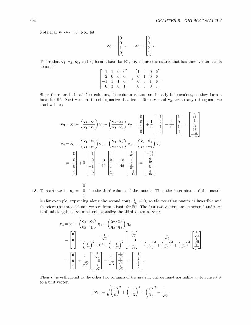
394 CHAPTER 5. ORTHOGONALITY
Note that v1 · v2 = 0. Now let
x3 =
0010
, x4 =
0001
.To see that v1, v2, x3, and x4 form a basis for R4, row-reduce the matrix that has these vectors as itscolumns:
1 1 0 02 0 0 0−1 1 1 0
0 3 0 1
→
1 0 0 00 1 0 00 0 1 00 0 0 1
.Since there are 1s in all four columns, the column vectors are linearly independent, so they form abasis for R4. Next we need to orthogonalize that basis. Since v1 and v2 are already orthogonal, westart with x3:
v3 = x3 −(v1 · x3
v1 · v1
)v1 −
(v2 · x3
v2 · v2
)v2 =
0010
+1
6
12−1
0
− 1
11
1013
=
566134966
− 311
v4 = x4 −
(v1 · x4
v1 · v1
)v1 −
(v2 · x4
v2 · v2
)v2 −
(v3 · x4
v3 · v3
)v3
=
0
0
0
1
+ 0
1
2
−1
0
− 3
11
1
0
1
3
+18
49
566134966
− 311
=
− 12
49649
0449
.
13. To start, we let x3 =
001
be the third column of the matrix. Then the determinant of this matrix
is (for example, expanding along the second row) 1√66= 0, so the resulting matrix is invertible and
therefore the three column vectors form a basis for R3. The first two vectors are orthogonal and eachis of unit length, so we must orthogonalize the third vector as well:
v3 = x3 −(q1 · x3
q1 · q1
)q1 −
(q2 · x3
q2 · q2
)q2
=
0
0
1
− − 1√2(
1√2
)2
+ 02 +(− 1√
2
)2
1√2
0
− 1√2
− 1√3(
1√3
)2
+(
1√3
)2
+(
1√3
)2
1√3
1√3
1√3
=
0
0
1
+1√2
1√2
0
− 1√2
− 1√3
1√3
1√3
1√3
=
16
− 1316
.Then v3 is orthogonal to the other two columns of the matrix, but we must normalize v3 to convert itto a unit vector.
‖v3‖ =
√(1
6
)2
+
(−1
3
)2
+
(1
6
)2
=1√6,

5.3. THE GRAM-SCHMIDT PROCESS AND THE QR FACTORIZATION 395
so that
q3 =1
1/√
6v3 =
1√6
− 2√6
1√6
,
so that the completed matrix Q is
Q =
1√2
1√3
1√6
0 1√3− 2√
6
− 1√2
1√3
1√6
.
14. To simplify the calculations, we will start with the multiples v1 =
1111
and v2 =
210−3
of the given
basis vectors (column vectors of Q). We will find an orthogonal basis containing those two vectors andthen normalize all four at the very end. Note that v1 and v2 are already orthogonal. If we choose
x3 =
0010
and x4 =
0001
,
then calculating the determinant of[v1 v2 x3 x4
], for example by expanding along the last column,
shows that the matrix is invertible, so that these four vectors form a basis for R4. We now need toorthogonalize the last two vectors:
p3 = x3 −(v1 · x3
v1 · v1
)v1 −
(v2 · x3
v2 · v2
)v2
=
0
0
1
0
− 1 · 0 + 1 · 0 + 1 · 1 + 1 · 01 · 1 + 1 · 1 + 1 · 1 + 1 · 1
1
1
1
1
− 2 · 0 + 1 · 0 + 0 · 1− 3 · 02 · 2 + 1 · 1 + 0 · 0− 3 · (−3)
2
1
0
−3
=
0
0
1
0
− 1
4
1
1
1
1
=1
4
−1
−1
3
−1
.

396 CHAPTER 5. ORTHOGONALITY
Now let v3 = 4p3 =
−1
−1
3
−1
, again avoiding fractions. Next,
v4 = x4 −(v1 · x4
v1 · v1
)v1 −
(v2 · x4
v2 · v2
)v2 −
(v3 · x4
v3 · v3
)v3
=
0
0
0
1
− 1 · 0 + 1 · 0 + 1 · 0 + 1 · 11 · 1 + 1 · 1 + 1 · 1 + 1 · 1
1
1
1
1
− 2 · 0 + 1 · 0 + 0 · 0− 3 · 12 · 2 + 1 · 1 + 0 · 0− 3 · (−3)
2
1
0
−3
− −1 · 0− 1 · 0 + 3 · 0− 1 · 1−1 · (−1)− 1 · (−1) + 3 · 3− 1 · (−1)
−1
−1
3
−1
=
0
0
0
1
− 1
4
1
1
1
1
+3
14
2
1
0
−3
+1
12
−1
−1
3
−1
=
221
− 542
0142
.We now normalize v1 through v4; note that we already have normalized forms for the first two.
‖v3‖ =√
12 + 12 + 32 + 12 = 2√
3
‖v4‖ =
√(2
21
)2
+
(− 5
42
)2
+ 02 +
(1
42
)2
=1√42,
so that the matrix is
Q =
12
2√14
−√
36
4√42
12
1√14
−√
36 − 5√
4212 0
√3
2 012 − 3√
14−√
36
1√42
.
15. From Exercise 9, ‖v1‖ =√
2, ‖v2‖ =√
62 , and ‖v3‖ = 2
√3
3 , so that
Q =[q1 q2 q3
]=
0 2√6
1√3
1√2− 1√
61√3
1√2
1√6− 1√
3
.Therefore
R = QTA =
0 1√2
1√2
2√6− 1√
61√6
1√3
1√3− 1√
3
0 1 1
1 0 1
1 1 0
=
√
2 1√2
1√2
0 3√6
1√6
0 0 2√3
.

5.3. THE GRAM-SCHMIDT PROCESS AND THE QR FACTORIZATION 397
16. From Exercise 10, ‖v1‖ = 2, ‖v2‖ = 2√
6, and ‖v3‖ =√
2, so that
Q =[q1 q2 q3
]=
12 0 012 −
√6
61√2
− 12
√6
61√2
12
√6
3 0
.
Therefore
R = QTA =
12
12 − 1
212
0 −√
66
√6
6
√6
3
0 1√2
1√2
0
1 1 1
1 −1 2
−1 1 0
1 5 1
=
2 2 2
0 2√
6 0
0 0√
2
.17. We have
R = QTA =
23
13 − 2
313
23
23
23 − 2
313
2 8 2
1 7 −1
−2 −2 1
=
3 9 13
0 6 23
0 0 73
18. We have
R = QTA =
[1√6
2√6− 1√
60
1√3
0 1√3
1√3
]1 3
2 4
−1 −1
0 1
=
[√6 2√
6
0√
3
].
19. If A is already orthogonal, let Q = A and R = I, which is upper triangular; then A = QR.
20. First, if A is invertible, then A has linearly independent columns, so that by Theorem 5.16, A = QRwhere R is invertible. Since R is upper triangular, its determinant is the product of its diagonal entries,so that R invertible implies that all of its diagonal entries are nonzero. For the converse, if R is uppertriangular with all diagonal entries nonzero, then it has nonzero determinant; since Q is orthogonal, itis invertible so has nonzero determinant as well. But then detA = det(QR) = (detQ)(detR) 6= 0, sothat A is invertible. Note that when this occurs,
A−1 = (QR)−1 = R−1Q−1 = R−1QT .
21. From Exercise 20, A−1 = R−1QT . To compute R−1, we row-reduce[R I
]using Exercise 15:
√2 1√
21√2
1 0 0
0 3√6
1√6
0 1 0
0 0 2√3
0 0 1
→
1 0 0√
22 −
√6
6 −√
36
0 1 0 0√
63 −
√3
6
0 0 1 0 0√
32
.Thus
A−1 = R−1QT =
√
22 −
√6
6 −√
36
0√
63 −
√3
6
0 0√
32
0 1√2
1√2
2√6− 1√
61√6
1√3
1√3− 1√
3
=
− 1
212
12
12 − 1
212
12
12 − 1
2
.22. From Exercise 20, A−1 = R−1QT . To compute R−1, we row-reduce
[R I
]using Exercise 17:3 9 1
3 1 0 0
0 6 23 0 1 0
0 0 73 0 0 1
→1 0 0 1
3 − 12
221
0 1 0 0 16 − 1
21
0 0 1 0 0 37
.

398 CHAPTER 5. ORTHOGONALITY
Thus
A−1 = R−1QT =
13 − 1
2221
0 16 − 1
21
0 0 37
23
13 − 2
313
23
23
23 − 2
313
=
542 − 2
7 − 1121
142
17
221
27 − 2
717
.23. If A = QR is a QR-factorization of A, then we want to show that Rx = 0 implies that x = 0 so that
R is invertible by part (c) of the Fundamental Theorem. Note that since Q is orthogonal, so is QT , sothat by Theorem 5.6(b),
∥∥QTx∥∥ = ‖x‖ for any vector x. Then
Rx = 0 ⇒ ‖Rx‖ = 0 ⇒∥∥(QTA)x
∥∥ =∥∥QT (Ax)
∥∥ = ‖Ax‖ = 0 ⇒ Ax = 0.
If ai are the columns of A, then Ax = 0 means that∑
aixi = 0. But this means that all of the xi arezero since the columns of A are linearly independent. Thus x = 0. By part (c) of the FundamentalTheorem, we conclude that R is invertible.
24. Recall that row(A) = row(B) if and only if there is an invertible matrix M such that A = MB. ThenA = QR implies that AT = RTQT ; since A has linearly independent columns, R is invertible, so thatRT is as well. Thus row(AT ) = row(QT ), so that col(A) = col(Q).
Exploration: The Modified QR Process
1. I − 2uuT = I − 2
[d1
d2
] [d1 d2
]= I −
[2d2
1 2d1d2
2d1d2 2d22
]=
[1− 2d2
1 −2d1d2
−2d1d2 1− 2d22
].
2. (a) From Exercise 1,
Q =
[1− 2d2
1 −2d1d2
−2d1d2 1− 2d22
]=
[1− 2 · 9
25 −2 · 35 ·
45
−2 · 35 ·
45 1− 2 · 16
25
]=
[725 − 24
25
− 2425 − 7
25
].
(b) Since ‖x− y‖ =√
(5− 1)2 + (5− 7)2 = 2√
5, we have
u =1
2√
5(x− y) =
[4
2√
5
− 22√
5
]=
[2√5
− 1√5
].
Then from Exercise 1,
Q =
[1− 2d2
1 −2d1d2
−2d1d2 1− 2d22
]=
1− 2 · 45 −2 · 2√
5·(− 1√
5
)−2 · 2√
5·(− 1√
5
)1− 2 · 1
5
=
[− 3
545
45
35
].
3. (a) QT = (I − 2uuT )T = I − 2(uuT
)T= I − 2
(uT)T
uT = I − 2uuT = Q, so that Q is symmetric.
(b) Start with
QQT = QQ = (I − 2uuT )(I − 2uuT ) = I − 4uuT +(−2uuT
)2= I − 4uuT + 4uuTuuT .
Now, uTu = u · u = 1 since u is a unit vector, so the equation above becomes
QQT = I − 4uuT + 4uuTuuT = I − 4uuT + 4uuT = I.
Thus QT = Q−1 and it follows that Q is orthogonal.
(c) This follows from parts (a) and (b): Q2 = QQ = QQT = QQ−1 = I.

Exploration: The Modified QR Process 399
4. First suppose that v is in the span of u; say v = cu. Then again using the fact that uTu = u · u = 1,
Qv = Q(cu) = (I − 2uuT )(cu) = c(u− 2uuTu) = c(u− 2u) = −cu = −v.
If v · u = uTv = 0, thenQv = (I − 2uuT )v = v − 2uuTv = v.
5. First normalize the given vector to get
u =
1√6
− 1√6
2√6
.Then
uuT =
16 − 1
613
− 16
16 − 1
313 − 1
323
, so that Q = I − 2uuT =
23
13 − 2
313
23
23
− 23
23 − 1
3
.For Exercise 3, clearly Q is symmetric, and each column has norm 1. A short computation shows thateach pair of columns is orthogonal. Therefore Q is orthogonal. Finally,
Q2 =
23
13 − 2
313
23
23
− 23
23 − 1
3
23
13 − 2
313
23
23
− 23
23 − 1
3
= I.
For Exercise 4, first suppose that v = cu. Then
Qv = Q(cu) = cQu = c
23
13 − 2
313
23
23
− 23
23 − 1
3
1√6
− 1√6
2√6
= c
− 1√
61√6
− 2√6
= −cu = −v.
If v · u = uTv = 0, then
[1√6− 1√
62√6
]x1
x2
x3
=1√6x1 −
1√6x2 +
2√6x3 = 0,
so that x1− x2 + 2x3 = 0 and therefore x2 = x1 + 2x3. Thus if v ·u = 0, then v = s
110
+ t
021
. But
then
Qv = Q
s1
1
0
+ t
0
2
1
= sQ
1
1
0
+ tQ
0
2
1
= s
23
13 − 2
313
23
23
− 23
23 − 1
3
1
1
0
+ t
23
13 − 2
313
23
23
− 23
23 − 1
3
0
2
1
= s
1
1
0
+ t
0
2
1
= v.

400 CHAPTER 5. ORTHOGONALITY
6. x− y is a multiple of u, so that Q(x− y) = −(x− y) by Exercise 4. Next,
(x + y) · u =1
‖x− y‖(x + y) · (x− y).
But by Exercise 61 in Section 1.2, this dot product is zero because ‖x‖ = ‖y‖. Thus x+y is orthogonalto u, so that Q(x + y) = x + y. So we have
Q(x− y) = −(x− y)
Q(x + y) = x + y⇒
Qx−Qy = −x + y
Qx +Qy = x + y⇒ 2Qx = 2y ⇒ Qx = y.
7. We have
u =1
‖x− y‖(x− y) =
1
2√
3
−222
,so that
uuT =
13 − 1
3 − 13
− 13
13
13
− 13
13
13
⇒ Q = I − 2uuT =
13
23
23
23
13 − 2
323 − 2
313
.Then
Qx =
13
23
23
23
13 − 2
323 − 2
313
1
2
2
=
3
0
0
= y.
8. Since ‖y‖ =
√‖x‖2 = ‖x‖, if ai is the ith column vector of A, we can apply Exercise 6 to get
Q1A =[Q1a1 Q1a2 . . . Q1an
]=[Q1x Q1a2 . . . Q1an
]=[y Q1a2 . . . Q1an
]=
[∗ ∗0 A1
],
since the last m− 1 entries in y are all zero. Here A1 is (m− 1)× (n− 1), the left-hand ∗ is 1× 1, andthe right-hand ∗ is 1× (n− 1).
9. Since P2 is a Householder matrix, it is orthogonal, so that
Q2QT2 =
[1 00 P2
] [1 00 PT2
]= I,
so that Q2 is orthogonal as well. Further,
Q2Q1A =
[1 00 P2
] [∗ ∗0 A1
]=
[∗ ∗0 P2A1
]=
∗ ∗ ∗0 ∗ ∗0 0 A2
.10. Using induction, suppose that
QkQk−1 · · ·Q1A =
∗ ∗ ∗0 ∗ ∗0 0 Ak
.Repeat Exercise 8 on the matrix Ak, giving a Householder matrix Pk+1 such that
Pk+1Ak =
[∗ ∗0 Ak+1
].

Exploration: The Modified QR Process 401
Let Qk+1 =
[1 00 Pk+1
]. Then using the fact that Pk+1 is orthogonal, we again conclude that Qk+1 is
orthogonal, and that
Qk+1QkQk−1 · · ·Q1A =
∗ ∗ ∗0 ∗ ∗0 0 Ak+1
.The result then follows by induction. The resulting matrix R = Qm−1 · · ·Q2Q1A is upper triangularby construction.
11. If Q = Q1Q2 · · ·Qm−1, then Q is orthogonal since each Qi is orthogonal, and
QT = (Q1Q2 · · ·Qm−1)T
= QTm−1 · · ·QT2 QT1 = Qm−1 · · ·Q2Q1.
Thus QTA = Qm−1 · · ·Q2Q1A = R, so that QQTA = A = QR, since QQT = I.
12. (a) We start with x =
[3−4
], so that y =
[√32 + (−4)2 = 5
0
]. Then
u =
[− 1√
5
− 2√5
]⇒ uuT =
[15
25
25
45
].
Then
Q1 = I − 2uuT =
[35 − 4
5
− 45 − 3
5
]⇒ Q1A =
[5 3 −1
0 −9 −2
]= R,
and A = QT1 R.
(b) We start with x =
122
, so that y =
300
. Then
u =
− 1√
31√3
1√3
⇒ uuT =
13 − 1
3 − 13
− 13
13
13
− 13
13
13
.Thus
Q1 = I − 2uuT =
13
23
23
23
13 − 2
323 − 2
313
⇒ Q1A =
3 −5 1 83
0 4 3 13
0 3 1 43
.Then
A1 =
[4 3 1
3
3 1 43
],
so that in the next iteration
x =
[4
3
]⇒ y =
[5
0
]⇒ u =
[− 1√
103√10
].
Then
uuT =
[110 − 3
10
− 310
910
].
So
P2 = I − 2uuT =
[45
35
35 − 4
5
]⇒ Q2 =
[1 0
0 P2
]=
1 0 0
0 45
35
0 35 − 4
5
.

402 CHAPTER 5. ORTHOGONALITY
Finally,
Q2Q1A =
1 0 0
0 45
35
0 35 − 4
5
3 −5 1 8
3
0 4 3 13
0 3 1 43
=
3 −5 1 83
0 5 3 1615
0 0 1 − 1315
= R,
and Q1Q2R = A.
Exploration: Approximating Eigenvalues with the QR Algorithm
1. We haveA1 = RQ = (Q−1Q)RQ = Q−1(QR)Q = Q−1AQ,
so that A1 ∼ A. Thus by Theorem 4.22(e), A1 and A have the same eigenvalues.
2. Using Gram-Schmidt, we have
v1 =
[1
1
]
v2 =
[0
3
]− 1 · 0 + 1 · 3
1 · 1 + 1 · 1
[1
1
]=
[0
3
]− 3
2
[1
1
]=
[− 3
232
].
Normalizing these vectors gives
Q =
[1√2
1√2
1√2− 1√
2
], so that R = QTA =
[√2 3
√2
2
0 − 3√
22
].
Thus
A1 = RQ =
[√2 3
√2
2
0 − 3√
22
][1√2
1√2
1√2− 1√
2
]=
[52 − 1
2
− 32
32
].
Then
det(A− λI) =
∣∣∣∣∣1− λ 0
1 3− λ
∣∣∣∣∣ = (1− λ)(3− λ)
det(A1 − λI) =
∣∣∣∣∣ 52 − λ − 12
− 32
32 − λ
∣∣∣∣∣ =
(5
2− λ)(
3
2− λ)− 3
4= λ2 − 4λ+ 3 = (λ− 1)(λ− 3).
So A and A1 do indeed have the same eigenvalues.
3. The proof is by induction on k. We know that A1 ∼ A. Now assume An−1 ∼ A. Then
An = Rn−1Qn−1 = (Q−1n−1Qn−1)Rn−1Qn−1 = Q−1
n−1(Qn−1Rn−1)Qn−1 = Q−1n−1An−1Qn−1,
so that An ∼ An−1 ∼ A.
4. Converting A1 = Q1R1 to decimals gives, using technology
A1 = Q1R1 ≈[
0.86 0.51−0.51 0.86
] [2.92 −1.20
0 1.04
]⇒ A2 = R1Q1 ≈
[3.12 0.47−0.53 0.88
]A2 = Q2R2 ≈
[−0.99 0.17
0.17 0.99
] [−3.16 −0.32
0 0.95
]⇒ A3 = R2Q2 ≈
[3.06 −0.840.16 0.93
]A3 = Q3R3 ≈
[−1.00 −0.05−0.05 1.00
] [−3.06 0.79
0 0.97
]⇒ A4 = R3Q3 ≈
[3.02 0.94−0.05 0.97
]A4 = Q4R4 ≈
[−1.00 0.02
0.02 1.00
] [−3.02 −0.92
0 0.99
]⇒ A5 = R4Q4 ≈
[3.00 −0.980.02 0.99
].
The Ak are approaching an upper triangular matrix U .

Exploration: Approximating Eigenvalues with the QR Algorithm 403
5. Since Ak ∼ A for all k, the eigenvalues of A and Ak are the same, so in the limit, the upper triangularmatrix U will have eigenvalues equal to those of A; but the eigenvalues of a triangular matrix are itsdiagonal entries. Thus the diagonal entries of U will be the eigenvalues of A.
6. (a) Follow the same process as in Exercise 4.
A = QR ≈[0.71 0.710.71 −0.71
] [2.83 2.83
0 1.41
]⇒ A1 = RQ ≈
[4.02 0.001.00 −1.00
]A1 = Q1R1 ≈
[−0.97 −0.24−0.24 0.97
] [−4.14 0.24
0 −0.97
]⇒ A2 = R1Q1 ≈
[3.96 1.230.23 −0.94
]A2 = Q2R2 ≈
[−1.00 −0.06−0.06 1.00
] [−3.97 −1.17
0 −1.01
]⇒ A3 = R2Q2 ≈
[4.04 −0.930.06 −1.01
]A3 = Q3R3 ≈
[−1.00 −0.01−0.01 1.00
] [−4.04 0.94
0 −1.00
]⇒ A4 = R3Q3 ≈
[4.03 0.980.01 −1.00
]A4 = Q4R4 ≈
[−1.00 0.00
0.00 1.00
] [−4.03 −0.98
0 −1.00
]⇒ A5 = R4Q4 ≈
[4.03 −0.980.00 −1.00
].
The eigenvalues of A are approximately 4.03 and −1.00.
(b) Follow the same process as in Exercise 4.
A = QR ≈[0.45 0.890.89 −0.45
] [2.24 1.34
0 0.45
]⇒ A1 = RQ ≈
[2.20 1.400.40 −0.20
]A1 = Q1R1 ≈
[−0.98 −0.18−0.18 0.98
] [−2.24 −1.34
0 −0.45
]⇒ A2 = R1Q1 ≈
[2.44 −0.920.08 −0.44
]A2 = Q2R2 ≈
[−1.00 −0.03−0.03 1.00
] [−2.44 0.93
0 −0.41
]⇒ A3 = R2Q2 ≈
[2.41 1.010.01 −0.41
]A3 = Q3R3 ≈
[−1 0
0 1
] [−2.41 −1.01
0 −0.42
]⇒ A4 = R3Q3 ≈
[2.42 −1
0 −0.42
]A4 = Q4R4 ≈
[−1.00 0.00
0.00 1.00
] [−2.42 1
0 −0.41
]⇒ A5 = R4Q4 ≈
[2.41 1
0 −0.41
].
The eigenvalues of A are approximately 2.41 and −0.41 (the true values are 1±√
2).
(c) Follow the same process as in Exercise 4.
A = QR ≈
0.24 −0.06 −0.970.24 0.97 0−0.94 0.23 −0.24
4.24 0.47 −0.940 1.94 1.260 0 0.73
⇒A1 = RQ ≈
2.00 0 −3.89−0.73 2.18 −0.31−0.69 0.17 −0.18
A1 = Q1R1 ≈
−0.89 −0.33 0.300.33 −0.94 −0.070.31 0.03 0.95
−2.24 0.76 3.320 −2.05 1.570 0 −1.31
⇒A2 = R1Q1 ≈
3.27 0.13 2.44−0.18 1.98 1.64−0.40 −0.04 −1.25
A2 = Q2R2 ≈
−0.99 −0.05 0.120.06 −1.00 0.010.12 0.02 0.99
−3.3 −0.03 −2.470 −1.99 −1.80 0 −1.31
⇒A3 = R2Q2 ≈
2.96 0.16 −2.86−0.33 1.95 −1.81−0.11 −0.02 −0.91

404 CHAPTER 5. ORTHOGONALITY
A3 = Q3R3 ≈
−0.99 −0.11 0.040.11 −0.99 0.010.04 0.01 1.00
−2.98 0.06 2.610 −1.95 2.100 0 −1.03
⇒A4 = R3Q3 ≈
3.07 0.30 2.49−0.14 1.96 2.09−0.04 −0.01 −1.03
A4 = Q4R4 ≈
−1 −0.04 0.010.04 −1 00.01 0 1
−3.07 −0.21 −2.410 −1.97 −2.200 0 −0.99
⇒A5 = R4Q4 ≈
3.03 0.34 −2.45−0.12 1.96 −2.21−0.01 0 −0.99
.The eigenvalues of A are approximately 3.03, 1.96, and −0.99. (The true values are 3, 2, and −1).
(d) Follow the same process as in Exercise 4.
A = QR ≈
0.45 0.720 0.60
−0.89 0.36
[2.24 −3.13 −2.240 3.35 0
]⇒ A1 = RQ ≈
[3.00 −1.07
0 2.00
]
A1 = Q1R1 ≈[1.00 0.000.00 1.00
] [3.00 −1.07
0 2.00
]⇒ A2 = R1Q1 ≈
[3.00 −1.07
0 2.00
].
Since Q1 is the identity matrix, we get Q2 = I and R2 = R1, so that successive Ai are equal toA1. Thus the eigenvalues of A are approximately 3 and 2 (in fact, they are 3, 2, and 0).
7. Following the process in Exercise 4,
A = QR =
[2√5− 1√
5
− 1√5− 2√
5
][√5 8√
5
0 1√5
]⇒ A1 = RQ =
[25 − 21
5
− 15 − 2
5
]
A1 = Q1R1 =
[2√5− 1√
5
− 1√5− 2√
5
][1√5− 8√
5
0√
5
]⇒ A2 = R1Q1 ≈
[2 3
−1 −2
]= A.
Here A2 = A (Q1 = Q−1 and R1 = R−1); the algorithm fails because the eigenvalues of A, which are±1, do not have distinct absolute values.
8. Set
B = A+ 0.9I =
[2.9 3−1 −1.1
].
Then
B = QR ≈[−0.95 0.33
0.33 0.95
] [−3.07 −3.19
0 −0.06
]⇒ B1 = RQ ≈
[1.86 −4.02−0.02 −0.06
]B1 = Q1R1 ≈
[−1 0.01
0.01 1
] [−1.86 4.02
0 −0.1
]⇒ B2 = R1Q1 ≈
[1.9 4
0 −0.1
]B2 = Q2R2 ≈
[−1.00 0
0 1.00
] [−1.9 −4
0 −0.1
]⇒ B3 = R2Q2 ≈
[1.9 −4
0 −0.1
].
Further iterations will simply reverse the sign of the upper right entry of Bi. The eigenvalues ofB are approximately 1.9 and −0.1, so the eigenvalues of A are approximately 1.9 − 0.9 = 1.0 and−0.1− 0.9 = −1.0. These are correct (see Exercise 7).

5.4. ORTHOGONAL DIAGONALIZATION OF SYMMETRIC MATRICES 405
9. We prove the first equality using induction on k. For k = 1, it says that Q0A1 = AQ0, or QA1 = AQ.Now, A1 = RQ and A = QR, so that QA1 = QRQ = (QR)Q = AQ. This proves the basis of theinduction. Assume the equality holds for k = n; we prove it for k = n+ 1:
Q0Q1Q2 · · ·QnAn+1 = Q0Q1Q2 · · ·Qn−1(QnAn+1)
= Q0Q1Q2 · · ·Qn−1(Qn(RnQn))
= Q0Q1Q2 · · ·Qn−1(QnRn)Qn
= (Q0Q1Q2 · · ·Qn−1An)Qn
= (AQ0Q1Q2 · · ·Qn−1)Qn
= AQ0Q1Q2 · · ·Qn.
For the second equality, note that Ak = QkRk, so that
Q0Q1Q2 · · ·Qk−1Ak = Q0Q1Q2 · · ·Qk−1QkRk = AQ0Q1Q2 · · ·Qk−1.
Multiply both sides by Rk−1 · · ·R2R1 to get
(Q0Q1Q2 · · ·Qk−1Qk)(RkRk−1 · · ·R2R1) = A(Q0Q1Q2 · · ·Qk−1)(Rk−1 · · ·R2R1),
as desired.
For the QR-decomposition of Ak+1, we again use induction. For k = 0, the equation says thatQ0R0 = A0+1 = A, which is true. Now assume the statement holds for k = n. Then using the firstequation in this exercise together with the fact that Ak = QkRk and the inductive hypothesis, we get
An+1 = A ·An
= A(Q0Q1 · · ·Qn−1)(Rn−1 · · ·R1R0)
= Q0Q1 · · ·Qn−1AnRn−1 · · ·R1R0
= Q0Q1 · · ·Qn−1QnRnRn−1 · · ·R1R0
= (Q0Q1 · · ·Qn)(RnRn−1 · · ·R1R0),
as desired.
5.4 Orthogonal Diagonalization of Symmetric Matrices
1. The characteristic polynomial of A is
det(A− λI) =
∣∣∣∣4− λ 11 4− λ
∣∣∣∣ = λ2 − 8λ+ 15 = (λ− 5)(λ− 3)
Thus the eigenvalues of A are λ1 = 3 and λ2 = 5. To find the eigenspace corresponding to λ1 = 3, werow-reduce [
A− 3I 0]
=
[1 1 01 1 0
]→[1 1 00 0 0
].
A basis for the eigenspace is given by
[−1
1
].
To find the eigenspace corresponding to λ2 = 5, we row-reduce
[A− 5I 0
]=
[−1 1 0
1 −1 0
]→[1 −1 00 0 0
].
A basis for the eigenspace is given by
[11
].
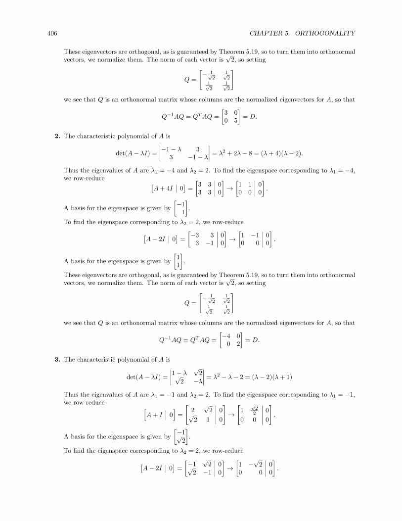
406 CHAPTER 5. ORTHOGONALITY
These eigenvectors are orthogonal, as is guaranteed by Theorem 5.19, so to turn them into orthonormalvectors, we normalize them. The norm of each vector is
√2, so setting
Q =
[− 1√
21√2
1√2
1√2
]
we see that Q is an orthonormal matrix whose columns are the normalized eigenvectors for A, so that
Q−1AQ = QTAQ =
[3 00 5
]= D.
2. The characteristic polynomial of A is
det(A− λI) =
∣∣∣∣−1− λ 33 −1− λ
∣∣∣∣ = λ2 + 2λ− 8 = (λ+ 4)(λ− 2).
Thus the eigenvalues of A are λ1 = −4 and λ2 = 2. To find the eigenspace corresponding to λ1 = −4,we row-reduce [
A+ 4I 0]
=
[3 3 03 3 0
]→[1 1 00 0 0
].
A basis for the eigenspace is given by
[−1
1
].
To find the eigenspace corresponding to λ2 = 2, we row-reduce[A− 2I 0
]=
[−3 3 0
3 −1 0
]→[1 −1 00 0 0
].
A basis for the eigenspace is given by
[11
].
These eigenvectors are orthogonal, as is guaranteed by Theorem 5.19, so to turn them into orthonormalvectors, we normalize them. The norm of each vector is
√2, so setting
Q =
[− 1√
21√2
1√2
1√2
]
we see that Q is an orthonormal matrix whose columns are the normalized eigenvectors for A, so that
Q−1AQ = QTAQ =
[−4 0
0 2
]= D.
3. The characteristic polynomial of A is
det(A− λI) =
∣∣∣∣1− λ √2√
2 −λ
∣∣∣∣ = λ2 − λ− 2 = (λ− 2)(λ+ 1)
Thus the eigenvalues of A are λ1 = −1 and λ2 = 2. To find the eigenspace corresponding to λ1 = −1,we row-reduce [
A+ I 0]
=
[2√
2 0√2 1 0
]→
[1
√2
2 0
0 0 0
].
A basis for the eigenspace is given by
[−1√
2
].
To find the eigenspace corresponding to λ2 = 2, we row-reduce[A− 2I 0
]=
[−1
√2 0√
2 −1 0
]→[1 −
√2 0
0 0 0
].
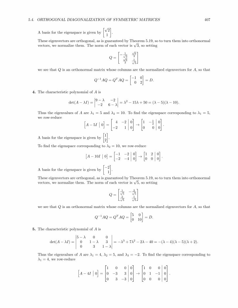
5.4. ORTHOGONAL DIAGONALIZATION OF SYMMETRIC MATRICES 407
A basis for the eigenspace is given by
[√2
1
].
These eigenvectors are orthogonal, as is guaranteed by Theorem 5.19, so to turn them into orthonormalvectors, we normalize them. The norm of each vector is
√3, so setting
Q =
[− 1√
3
√6
3√6
31√3
]
we see that Q is an orthonormal matrix whose columns are the normalized eigenvectors for A, so that
Q−1AQ = QTAQ =
[−1 0
0 2
]= D.
4. The characteristic polynomial of A is
det(A− λI) =
∣∣∣∣9− λ −2−2 6− λ
∣∣∣∣ = λ2 − 15λ+ 50 = (λ− 5)(λ− 10).
Thus the eigenvalues of A are λ1 = 5 and λ2 = 10. To find the eigenspace corresponding to λ1 = 5,we row-reduce [
A− 5I 0]
=
[4 −2 0
−2 1 0
]→
[1 − 1
2 0
0 0 0
].
A basis for the eigenspace is given by
[12
].
To find the eigenspace corresponding to λ2 = 10, we row-reduce
[A− 10I 0
]=
[−1 −2 0−2 −4 0
]→[1 2 00 0 0
].
A basis for the eigenspace is given by
[−2
1
].
These eigenvectors are orthogonal, as is guaranteed by Theorem 5.19, so to turn them into orthonormalvectors, we normalize them. The norm of each vector is
√5, so setting
Q =
[1√5− 2√
52√5
1√5
]
we see that Q is an orthonormal matrix whose columns are the normalized eigenvectors for A, so that
Q−1AQ = QTAQ =
[5 00 10
]= D.
5. The characteristic polynomial of A is
det(A− λI) =
∣∣∣∣∣∣5− λ 0 0
0 1− λ 30 3 1− λ
∣∣∣∣∣∣ = −λ3 + 7λ2 − 2λ− 40 = −(λ− 4)(λ− 5)(λ+ 2).
Thus the eigenvalues of A are λ1 = 4, λ2 = 5, and λ3 = −2. To find the eigenspace corresponding toλ1 = 4, we row-reduce
[A− 4I 0
]=
1 0 0 0
0 −3 3 0
0 3 −3 0
→1 0 0 0
0 1 −1 0
0 0 0 0
.

408 CHAPTER 5. ORTHOGONALITY
A basis for the eigenspace is given by
011
.
To find the eigenspace corresponding to λ2 = 5, we row-reduce
[A− 5I 0
]=
0 0 0 00 −4 3 00 3 −4 0
→0 1 0 0
0 0 1 00 0 0 0
.A basis for the eigenspace is given by
100
.
To find the eigenspace corresponding to λ3 = −2, we row-reduce
[A+ 2I 0
]=
7 0 0 00 3 3 00 3 3 0
→1 0 0 0
0 1 1 00 0 0 0
.A basis for the eigenspace is given by
0−1
1
.
These eigenvectors are orthogonal, as is guaranteed by Theorem 5.19, so to turn them into orthonormalvectors, we normalize them. The norm of the first and third vectors is
√2, while the second is already
a unit vector, so setting
Q =
0 1 0
1√2
0 − 1√2
1√2
0 1√2
we see that Q is an orthonormal matrix whose columns are the normalized eigenvectors for A, so that
Q−1AQ = QTAQ =
4 0 00 5 00 0 −2
= D.
6. The characteristic polynomial of A is
det(A− λI) =
∣∣∣∣∣∣2− λ 3 0
3 2− λ 40 4 2− λ
∣∣∣∣∣∣ = −λ3 + 6λ2 + 13λ− 42 = −(λ+ 3)(λ− 2)(λ− 7).
Thus the eigenvalues of A are λ1 = −3, λ2 = 2, and λ3 = 7. To find the eigenspace corresponding toλ1 = −3, we row-reduce
[A+ 3I 0
]=
5 3 0 0
3 5 4 0
0 4 5 0
→
1 0 − 34 0
0 1 54 0
0 0 0 0
.
A basis for the eigenspace is given (after clearing fractions) by
3−5
4
.
To find the eigenspace corresponding to λ2 = 2, we row-reduce
[A− 2I 0
]=
0 3 0 0
3 0 4 0
0 4 0 0
→
1 0 43 0
0 1 0 0
0 0 0 0
.

5.4. ORTHOGONAL DIAGONALIZATION OF SYMMETRIC MATRICES 409
A basis for the eigenspace is given (after clearing fractions) by
−403
.
To find the eigenspace corresponding to λ3 = 7, we row-reduce
[A− 7I 0
]=
−5 3 0 0
3 −5 4 0
0 4 −5 0
→
1 0 − 34 0
0 1 − 54 0
0 0 0 0
.
A basis for the eigenspace is given (after clearing fractions) by
354
.
These eigenvectors are orthogonal, as is guaranteed by Theorem 5.19, so to turn them into orthonormalvectors, we normalize them. The norms of these vectors are respectively 5
√2, 5, and 5
√2, so setting
Q =
3
5√
2− 4
53
5√
2
− 1√2
0 1√2
45√
235
45√
2
we see that Q is an orthonormal matrix whose columns are the normalized eigenvectors for A, so that
Q−1AQ = QTAQ =
−3 0 00 2 00 0 7
= D.
7. The characteristic polynomial of A is
det(A− λI) =
∣∣∣∣∣∣1− λ 0 −1
0 1− λ 0−1 0 1− λ
∣∣∣∣∣∣ = −λ3 + 3λ2 − 2λ = −λ(λ− 1)(λ− 2).
Thus the eigenvalues of A are λ1 = 0, λ2 = 1, and λ3 = 2. To find the eigenspace corresponding toλ1 = 0, we row-reduce
[A− 0I 0
]=
1 0 −1 0
0 1 0 0
−1 0 1 0
→1 0 −1 0
0 1 0 0
0 0 0 0
.
A basis for the eigenspace is given by
101
.
To find the eigenspace corresponding to λ2 = 1, we row-reduce
[A− I 0
]=
0 0 −1 00 0 0 0−1 0 0 0
→1 0 0 0
0 0 1 00 0 0 0
.A basis for the eigenspace is given by
010
.
To find the eigenspace corresponding to λ3 = 2, we row-reduce
[A− 2I 0
]=
−1 0 −1 00 −1 0 0−1 0 −1 0
→1 0 1 0
0 1 0 00 0 0 0
.

410 CHAPTER 5. ORTHOGONALITY
A basis for the eigenspace is given by
−101
.
These eigenvectors are orthogonal, as is guaranteed by Theorem 5.19, so to turn them into orthonormalvectors, we normalize them. The norm of the first and third vectors is
√2, while the second is already
a unit vector, so setting
Q =
1√2
0 − 1√2
0 1 01√2
0 1√2
we see that Q is an orthonormal matrix whose columns are the normalized eigenvectors for A, so that
Q−1AQ = QTAQ =
0 0 00 1 00 0 2
= D.
8. The characteristic polynomial of A is
det(A− λI) =
∣∣∣∣∣∣1− λ 2 2
2 1− λ 22 2 1− λ
∣∣∣∣∣∣ = −λ3 + 3λ2 + 9λ+ 5 = −(λ+ 1)2(λ− 5)
Thus the eigenvalues of A are λ1 = −1 and λ2 = 5. To find the eigenspace E−1 corresponding toλ1 = −1, we row-reduce
[A+ I 0
]=
2 2 2 02 2 2 02 2 2 0
→1 1 1 0
0 0 0 00 0 0 0
.Thus the eigenspace E−1 is−s− ts
t
= span
x1 =
−110
, x2 =
−101
.
To find the eigenspace E5 corresponding to λ2 = 5, we row-reduce
[A− 5I 0
]=
−4 2 2 02 −4 2 02 2 −4 0
→1 0 −1 0
0 1 −1 00 0 0 0
.Thus a basis for E5 is v3 =
111
.
E5 is orthogonal to E−1 as guaranteed by Theorem 10.19, so to turn this basis into an orthogonal basiswe must orthogonalize the basis for E−1 above. Use Gram-Schmidt:
v1 =
−110
, v2 = x2 −(v1 · x2
v1 · v1
)v1 =
−101
− 1
2
−110
=
− 1
2
− 12
1
.We double v2 to remove fractions, so we get the orthogonal basis
v1 =
−110
, v2 =
−1−1
2
, v3 =
111

5.4. ORTHOGONAL DIAGONALIZATION OF SYMMETRIC MATRICES 411
The norms of these vectors are, respectively,√
2,√
6, and√
3, so normalizing each vector and settingQ equal to the matrix whose columns are the normalized eigenvectors gives
Q =
− 1√
2− 1√
61√3
1√2− 1√
61√3
0 2√6
1√3
,so that
Q−1AQ = QTAQ =
−1 0 00 −1 00 0 5
= D.
9. The characteristic polynomial of A is
det(A− λI) =
∣∣∣∣∣∣∣∣1− λ 1 0 0
1 1− λ 0 00 0 1− λ 10 0 1 1− λ
∣∣∣∣∣∣∣∣ = λ4 − 4λ3 + 4λ2 = λ2(λ− 2)2.
Thus the eigenvalues of A are λ1 = 0 and λ2 = 2. To find the eigenspace E0 corresponding to λ1 = 0,we row-reduce
[A+ 0I 0
]=
1 1 0 0 01 1 0 0 00 0 1 1 00 0 1 1 0
→
1 1 0 0 00 0 1 1 00 0 0 0 00 0 0 0 0
.Thus the eigenspace E0 is
−ss−tt
= span
x1 =
−1
100
, x2 =
00−1
1
.
To find the eigenspace E2 corresponding to λ2 = 2, we row-reduce
[A− 2I 0
]=
−1 1 0 0 0
1 −1 0 0 00 0 −1 1 00 0 1 −1 0
→
1 −1 0 0 00 0 1 −1 00 0 0 0 00 0 0 0 0
.Thus the eigenspace E2 is
sstt
= span
x3 =
1100
, x4 =
0011
.
E0 is orthogonal to E2 as guaranteed by Theorem 10.19, and x1 and x2 are also orthogonal, as are x3
and x4. So these four vectors form an orthogonal basis. The norm of each vector is√
2, so normalizingeach vector and setting Q equal to the matrix whose columns are the normalized eigenvectors gives
Q =
− 1√
20 1√
20
1√2
0 1√2
0
0 − 1√2
0 1√2
0 1√2
0 1√2

412 CHAPTER 5. ORTHOGONALITY
so that
Q−1AQ = QTAQ =
0 0 0 00 0 0 00 0 2 00 0 0 2
= D.
10. The characteristic polynomial of A is
det(A− λI) =
∣∣∣∣∣∣∣∣2− λ 0 0 1
0 1− λ 0 00 0 1− λ 01 0 0 2− λ
∣∣∣∣∣∣∣∣ = λ4 − 6λ3 + 12λ2 − 10λ+ 3 = (λ− 1)3(λ− 3)
Thus the eigenvalues of A are λ1 = 1 and λ2 = 3. To find the eigenspace E1 corresponding to λ1 = 1,we row-reduce
[AI 0
]=
1 0 0 1 00 0 0 0 00 0 0 0 01 0 0 1 0
→
1 0 0 1 00 0 0 0 00 0 0 0 00 0 0 0 0
.Thus the eigenspace E1 is
−stus
= span
−1
001
,
0100
,
0010
.
Note that these vectors are mutually orthogonal.
To find the eigenspace E3 corresponding to λ2 = 3, we row-reduce
[A− 3I 0
]=
−1 0 0 1 0
0 −2 0 0 00 0 −2 0 01 0 0 −1 0
→
1 0 0 −1 00 1 0 0 00 0 1 0 00 0 0 0 0
.
Thus a basis for E3 is
1001
.
Since the eigenvectors of E1 are orthogonal to those of E3 by Theorem 10.19, and the eigenvectors ofE3 are already mutually orthogonal, all we need to do is to normalize the vectors. The norms are,respectively,
√2, 1, 1, and
√2, so setting Q equal to the matrix whose columns are the normalized
eigenvectors gives
Q =
− 1√
20 0 1√
2
0 1 0 0
0 0 1 01√2
0 0 1√2
,so that
Q−1AQ = QTAQ =
1 0 0 00 1 0 00 0 1 00 0 0 3
= D.
11. The characteristic polynomial is
det(A− λI) =
∣∣∣∣a− λ bb a− λ
∣∣∣∣ = (a− λ)2 − b2.

5.4. ORTHOGONAL DIAGONALIZATION OF SYMMETRIC MATRICES 413
This is zero when a − λ = ±b, so the eigenvalues are a + b and a − b. To find the correspondingeigenspaces, row-reduce: [
A− (a+ b)I 0]
=
[−b b 0b −b 0
]→[1 −1 00 0 0
][A− (a− b)I 0
]=
[b b 0b b 0
]→[1 1 00 0 0
].
So bases for the two eigenspaces (which are orthogonal by Theorem 5.19) are
[11
]and
[−1
1
]. Each of
these vectors has norm√
2, so normalizing each gives
Q =
[1√2− 1√
21√2
1√2
],
so that
Q−1AQ = QTAQ =
[a+ b 0
0 a− b
].
12. The characteristic polynomial is (expanding along the second row)
det(A− λI) =
∣∣∣∣∣∣a− λ 0 b
0 a− λ 0b 0 a− λ
∣∣∣∣∣∣ = (a− λ)((a− λ)2 − b2
).
This is zero when a = λ or when a − λ = ±b, so the eigenvalues are a, a + b and a − b. To find thecorresponding eigenspaces, row-reduce:
[A− aI 0
]=
0 0 b 00 0 0 0b 0 0 0
→1 0 0 0
0 0 1 00 0 0 0
[A− (a+ b)I 0
]=
−b 0 b 00 −b 0 0b 0 −b 0
→1 0 −1 0
0 1 0 00 0 0 0
[A− (a− b)I 0
]=
b 0 b 00 b 0 0b 0 b 0
→1 0 1 0
0 1 0 00 0 0 0
.So bases for the three eigenspaces (which are orthogonal by Theorem 5.19) are
010
,
101
and
−101
.
Normalizing the second and third vectors gives
Q =
0 1√
2− 1√
2
1 0 0
0 1√2
1√2
,so that
Q−1AQ = QTAQ =
a 0 00 a+ b 00 0 a− b
.13. (a) Since A and B are each orthogonally diagonalizable, they are each symmetric by the Spectral
Theorem. Therefore A + B is also symmetric, so it too is orthogonally diagonalizable by theSpectral Theorem.

414 CHAPTER 5. ORTHOGONALITY
(b) Since A is orthogonally diagonalizable, it is symmetric by the Spectral Theorem. Therefore cA isalso symmetric, so it too is orthogonally diagonalizable by the Spectral Theorem.
(c) Since A is orthogonally diagonalizable, it is symmetric by the Spectral Theorem. ThereforeA2 = AA is also symmetric, so it too is orthogonally diagonalizable by the Spectral Theorem.
14. If A is invertible and orthogonally diagonalizable, then QTAQ = D for some invertible diagonal matrixD and orthogonal matrix Q, so that
D−1 =(QTAQ
)−1= Q−1A−1
(QT)−1
= QTA−1(QT)T
= QTA−1Q.
Thus A−1 is also orthogonally diagonalizable (and by the same orthogonal matrix).
15. Since A and B are orthogonally diagonalizable, they are both symmetric. Since AB = BA, Exercise36 in Section 3.2 implies that AB is also symmetric, so it is orthogonally diagonalizable as well.
16. Let A be a symmetric matrix. Then it is orthogonally diagonalizable, say D = QTAQ. Then thediagonal entries of D are the eigenvalues of A. First, if every eigenvalue of A is nonnegative, let
D =
λ1 · · · 0...
. . ....
0 · · · λn
, and define√D =
√λ1 · · · 0...
. . ....
0 · · ·√λn
.Let B = Q
√DQT . Then B is diagonally orthogonalizable by construction, so it is symmetric. Further,
since Q is orthogonal,
B2 = Q√DQTQ
√DQT = Q
√DQ−1Q
√DQT = Q
√D√DQT = QDQT = A.
Conversely, suppose A = B2 for some symmetric matrix B. Then B is orthogonally diagonalizable,say QTBQ = D, so that
QTAQ = QTB2Q = (QTBQ)(QTBQ) = D2.
But D2 is a diagonal matrix whose diagonal entries are the squares of the diagonal entries of D, sothey are all nonnegative. Thus the eigenvalues of A are all nonnegative.
17. From Exercise 1 we have
λ1 = 3, q1 =
[− 1√
21√2
], λ2 = 5, q2 =
[1√2
1√2
].
Therefore
A = λ1q1qT1 + λ2q2q
T2 = 3
[12 − 1
2
− 12
12
]+ 5
[12
12
12
12
].
18. From Exercise 2 we have
λ1 = −4, q1 =
[− 1√
21√2
], λ2 = 2, q2 =
[1√2
1√2
].
Therefore
A = λ1q1qT1 + λ2q2q
T2 = −4
[12 − 1
2
− 12
12
]+ 2
[12
12
12
12
].
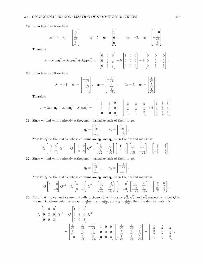
5.4. ORTHOGONAL DIAGONALIZATION OF SYMMETRIC MATRICES 415
19. From Exercise 5 we have
λ1 = 4, q1 =
01√2
1√2
, λ2 = 5, q2 =
1
0
0
, λ3 = −2, q2 =
0
− 1√2
1√2
.Therefore
A = λ1q1qT1 + λ2q2q
T2 + λ3q3q
T3 = 4
0 0 0
0 12
12
0 12
12
+ 5
1 0 0
0 0 0
0 0 0
− 2
0 0 0
0 12 − 1
2
0 − 12
12
.20. From Exercise 8 we have
λ1 = −1, q1 =
− 1√
21√2
0
, q2 =
− 1√
6
− 1√6
2√6
, λ2 = 5, q3 =
1√3
1√3
1√3
.Therefore
A = λ1q1qT1 + λ1q2q
T2 + λ2q3q
T3 = −
12 − 1
2 0
− 12
12 0
0 0 0
−
16
16 − 1
316
16 − 1
3
− 13 − 1
323
+ 5
13
13
13
13
13
13
13
13
13
.21. Since v1 and v2 are already orthogonal, normalize each of them to get
q1 =
[1√2
1√2
], q2 =
[1√2
− 1√2
].
Now let Q be the matrix whose columns are q1 and q2; then the desired matrix is
Q
[−1 0
0 2
]Q−1 = Q
[−1 0
0 2
]QT =
[1√2
1√2
1√2− 1√
2
][−1 0
0 2
][1√2
1√2
1√2− 1√
2
]=
[12 − 3
2
− 32
12
].
22. Since v1 and v2 are already orthogonal, normalize each of them to get
q1 =
[1√5
2√5
], q2 =
[− 2√
51√5
].
Now let Q be the matrix whose columns are q1 and q2; then the desired matrix is
Q
[3 0
0 −3
]Q−1 = Q
[3 0
0 −3
]QT =
[1√5− 2√
52√5
1√5
][3 0
0 −3
][1√5
2√5
− 2√5
1√5
]=
[− 9
5125
125
95
].
23. Note that v1, v2, and v3 are mutually orthogonal, with norms√
2,√
3, and√
6 respectively. Let Q bethe matrix whose columns are q1 = v1
‖v1‖ , q2 = v2
‖v2‖ , and q3 = v3
‖v3‖ ; then the desired matrix is
Q
1 0 0
0 2 0
0 0 3
Q−1 = Q
1 0 0
0 2 0
0 0 3
QT
=
1√2
1√3− 1√
61√2− 1√
31√6
0 1√3
2√6
1 0 0
0 2 0
0 0 3
1√2
1√2
01√3− 1√
31√3
− 1√6
1√6
2√6
=
53 − 2
3 − 13
− 23
53
13
− 13
13
83
.

416 CHAPTER 5. ORTHOGONALITY
24. Note that v1, v2, and v3 are mutually orthogonal, with norms√
42,√
3, and√
14 respectively. Let Qbe the matrix whose columns are q1 = v1
‖v1‖ , q2 = v2
‖v2‖ , and q3 = v3
‖v3‖ ; then the desired matrix is
Q
1 0 0
0 −4 0
0 0 −4
Q−1 = Q
1 0 0
0 −4 0
0 0 −4
QT
=
4√42− 1√
32√14
5√42
1√3− 1√
14
− 1√42
1√3
3√14
1 0 0
0 −4 0
0 0 −4
4√42
5√42− 1√
42
− 1√3
1√3
1√3
2√14− 1√
143√14
=
− 44
215021 − 10
215021 − 43
42 − 2542
− 1021 − 25
42 − 16342
.
25. Since q is a unit vector, q · q = 1, so that
projW v =
(q · vq · q
)q = (q · v)q = q(q · v) = q(qTv) = (qqT )v.
26. (a) By definition (see Section 5.2), the projection of v onto W is
projW v =
(q1 · vq1 · q1
)q1 + · · ·+
(qk · vqk · qk
)qk
= (q1 · v)q1 + · · ·+ (qk · v)qk
= q1(q1 · v) + · · ·+ qk(qk · v)
= q1(qT1 v) + · · ·+ qk(qTk · v)
= (q1qT1 + · · ·+ qkq
Tk )v.
Therefore the matrix of the projection is indeed q1qT1 + · · ·+ qkq
Tk .
(b) First,
PT = (q1qT1 + · · ·+ qkq
Tk )T =
(q1q
T1
)T+ · · ·+
(qkq
Tk
)T=(qT1)T
qT1 + · · ·+(qTk)T
qk = q1qT1 + · · ·+ qkq
Tk = P.
Next, since qi · qj = 0 for i 6= j, and qi · qi = qTi qi = 1, we have
P 2 = (q1qT1 )(q1q
T1 ) + · · ·+ (qkq
Tk )(qkq
Tk )
= q1
(qT1 q1
)qT1 + · · ·+ qk
(qTk qk
)qTk = q1q
T1 + · · ·qkqTk = P.
(c) We have
QQT =[q1 · · · qk
] qT1...qTk
= q1qT1 + · · ·qkqTk = P.
Thus rank(P ) = rank(QQT ) = rank(Q) by Theorem 3.28 in Section 3.5. But if q1, . . . ,qk is anorthonormal basis, then rank(Q) = k, so that rank(P ) = k as well.
5.5. APPLICATIONS 417
27. Suppose the eigenvalues are λ1, . . . , λn and that v1, . . . ,vn are a corresponding orthonormal set ofeigenvectors. Let Q1 =
[v1 · · · vn
]. Then
QT1 AQ1 =
vT1...vTn
A [v1 · · · vn]
=
vT1...vTn
[Av1 · · · Avn]
=
vT1...vTn
[λ1v1 · · · λnvn]
=
[λ1 ∗0 A1
]= T,
where A1 is an (n − 1) × (n − 1) matrix. The result now follows by induction since T is block uppertriangular.
28. We know that if A is nilpotent, then its only eigenvalue is 0. So if A is nilpotent, then all of itseigenvalues are real, so that by Exercise 27 there is an orthogonal matrix Q such that QTAQ is uppertriangular. But A and QTAQ have the same eigenvalues; since the eigenvalues of QTAQ are thediagonal entries, all the diagonal entries must be zero.
5.5 Applications
1. f(x) = xTAx =
[xy
] [2 33 4
] [x y
]= 2x2 + 6xy + 4y2.
2. f(x) = xTAx =
[x1
x2
] [5 11 −1
] [x1 x2
]= 5x2
1 + 2x1x2 − x22.
3. f(x) = xTAx =
[16
] [3 −2−2 4
] [1 6
]= 3 · 12 − 4 · 1 · 6 + 4 · 62 = 123.
4. f(x) =
xyz
1 0 −30 2 1−3 1 3
[x y z]
= 1x2 +2y2 +3z2 +0xy−6xz+2yz = x2 +2y2 +3z2−6xz+2yz.
5. From Exercise 4,
f
2−1
1
= 22 + 2 · (−1)2 + 3 · 12 − 6 · 2 · 1 + 2 · (−1) · 1 = −5.
6. f(x) = xTAx =
123
2 2 02 0 10 1 1
[1 2 3]
= 2 · 12 + 0 · 22 + 1 · 32 + 4 · 1 · 2 + 0 · 1 · 3 + 2 · 2 · 3 = 31.
7. The diagonal entries are 1 and 2, and the corners are each 12 · 6 = 3, so A =
[1 33 2
].
8. The diagonal entries are both zero, and the corners are each 12 · 1 = 1
2 , so A =
[0 1
212 0
].
9. The diagonal entries are 3 and −1, and the corners are each 12 · (−3) = − 3
2 , so A =
[3 − 3
2− 3
2 −1
].
10. The diagonal entries are 1, 0, and −1, while the off-diagonal entries are 12 · 8 = 4, 0, and 1
2 · (−6) = −3.Thus
A =
1 4 04 0 −30 −3 −1
.

418 CHAPTER 5. ORTHOGONALITY
11. The diagonal entries are 5, −1, and 2, while the off-diagonal entries are 12 · 2 = 1, 1
2 · (−4) = −2, and12 · 4 = 2. Thus
A =
5 1 −21 −1 2−2 2 2
.12. The diagonal entries are 2, −3, and 1, while the off-diagonal entries are 1
2 · 0 = 0, 12 · (−4) = −2, and
12 · 0 = 0. Thus
A =
2 0 −20 −3 0−2 0 1
.13. The matrix of this form is A =
[2 −2−2 5
], so that its characteristic polynomial is
∣∣∣∣2− λ −2−2 5− λ
∣∣∣∣ = λ2 − 7λ+ 6 = (λ− 1)(λ− 6).
So the eigenvalues are 1 and 6; finding the eigenvectors by the usual method gives corresponding
eigenvectors v1 =
[21
]and v2 =
[1−2
]. Normalizing these and constructing Q gives
Q =
[2√5
1√5
1√5− 2√
5
].
The new quadratic form is
f(y) = yTDy =[y1 y2
] [1 00 6
] [y1
y2
]= y2
1 + 6y22 .
14. The matrix of this form is A =
[1 44 1
], so that its characteristic polynomial is
∣∣∣∣1− λ 44 1− λ
∣∣∣∣ = λ2 − 2λ− 15 = (λ− 5)(λ+ 3).
So the eigenvalues are 5 and −3; finding the eigenvectors by the usual method gives corresponding
eigenvectors v1 =
[11
]and v2 =
[1−1
]. Normalizing these and constructing Q gives
Q =
[1√2
1√2
1√2− 1√
2
].
The new quadratic form is
f(y) = yTDy =[y1 y2
] [5 00 −3
] [y1
y2
]= 5y2
1 − 3y22 .
15. The matrix of this form is A =
7 4 44 1 −84 −8 1
, so that its characteristic polynomial is
∣∣∣∣∣∣7− λ 4 4
4 1− λ −84 −8 1− λ
∣∣∣∣∣∣ = (λ− 9)2(λ+ 9).

5.5. APPLICATIONS 419
So the eigenvalues are 9 (of algebraic multiplicity 2) and −9; finding the eigenvectors by the usual
method gives corresponding eigenvectors v1 =
201
and v2 =
210
for λ = 9 and
−122
for λ = −9.
Orthogonalizing v1 and v2 gives
v′2 = v2 −(v2 · v1
v1 · v1
)v1 =
210
− 4
5
201
=
251− 4
5
.Normalizing these and constructing Q gives
Q =
2√5
23√
5− 1
3
0 53√
523
1√5− 4
3√
523
.The new quadratic form is
f(y) = yTDy =[y1 y2 y3
] 9 0 00 9 00 0 −9
y1
y2
y3
= 9y21 + 9y2
2 − 9y23 .
16. The matrix of this form is A =
1 −2 0−2 1 0
0 0 3
, so that its characteristic polynomial is
∣∣∣∣∣∣1− λ −2 0−2 1− λ 00 0 3− λ
∣∣∣∣∣∣ = (λ− 3)2(λ+ 1).
So the eigenvalues are 3 (of algebraic multiplicity 2) and −1; finding the eigenvectors by the usual
method gives corresponding eigenvectors v1 =
1−1
0
and v2 =
001
for λ = 3 and
110
for λ = −1.
Since v1 and v2 are already orthogonal, we normalize all three vectors and construct Q to get
Q =
1√2
0 1√2
− 1√2
0 1√2
0 1 0
.The new quadratic form is
f(y) = yTDy =[y1 y2 y3
] 3 0 00 3 00 0 −1
y1
y2
y3
= 3y21 + 3y2
2 − y23 .
17. The matrix of this form is A =
1 −1 0−1 0 1
1 1 1
, so that its characteristic polynomial is
∣∣∣∣∣∣1− λ −1 0−1 −λ 11 1 1− λ
∣∣∣∣∣∣ = (λ− 2)(λ− 1)(λ+ 1).

420 CHAPTER 5. ORTHOGONALITY
So the eigenvalues are 2, 1, and −1; finding the eigenvectors by the usual method gives corresponding
eigenvectors v1 =
1−1−1
, v2 =
101
, and
12−1
. Normalize all three vectors and construct Q to get
Q =
1√3
1√2
1√6
− 1√3
0 2√6
− 1√3
1√2− 1√
6
.The new quadratic form is
f(x′) = (x′)TDx′ =[x′ y′ z′
] 2 0 00 1 00 0 −1
x′y′z′
= 2(x′)2 + (y′)2 − (z′)2.
18. The matrix of this form is A =
0 1 11 0 11 1 0
, so that its characteristic polynomial is
∣∣∣∣∣∣−λ 1 11 −λ 11 1 −λ
∣∣∣∣∣∣ = (λ− 2)(λ+ 1)2.
So the eigenvalues are 2 and −1; finding the eigenvectors by the usual method gives corresponding
eigenvectors v1 =
111
for λ = 2 and v2 =
−211
and v3 =
01−1
for λ = −1. The latter two are
already orthogonal, so simply normalize all three vectors and construct Q to get
Q =
1√3− 2√
60
1√3
1√6
1√2
1√3
1√6− 1√
2
.The new quadratic form is
f(x′) = (x′)TDx′ =[x′ y′ z′
] 2 0 00 −1 00 0 −1
x′y′z′
= 2(x′)2 − (y′)2 − (z′)2.
19. The matrix of this form is A =
[1 00 2
], so that its characteristic polynomial is
∣∣∣∣1− λ 00 2− λ
∣∣∣∣ = (1− λ)(2− λ).
Since the eigenvalues, 1 and 2, are both positive, this is a positive definite form.
20. The matrix of this form is A =
[1 −1−1 1
], so that its characteristic polynomial is
∣∣∣∣1− λ −1−1 1− λ
∣∣∣∣ = λ(λ− 2).
Since the eigenvalues, 0 and 2, are both nonnegative, but one is zero, this is a positive semidefiniteform.
5.5. APPLICATIONS 421
21. The matrix of this form is A =
[−2 1
1 −2
], so that its characteristic polynomial is
∣∣∣∣−2− λ 11 −2− λ
∣∣∣∣ = (λ+ 3)(λ+ 1).
Since the eigenvalues, −1 and −3, are both negative, this is a negative definite form.
22. The matrix of this form is A =
[1 22 1
], so that its characteristic polynomial is
∣∣∣∣1− λ 22 1− λ
∣∣∣∣ = (λ− 3)(λ+ 1).
Since the eigenvalues, −1 and 3, have opposite signs, this is an indefinite form.
23. The matrix of this form is A =
2 1 11 2 11 1 2
, so that its characteristic polynomial is
∣∣∣∣∣∣2− λ 1 1
1 2− λ 11 1 2− λ
∣∣∣∣∣∣ = −(λ− 1)2(λ− 4).
Since both eigenvalues, 1 and 4, are positive, this is a positive definite form.
24. The matrix of this form is A =
1 0 10 1 01 0 1
, so that its characteristic polynomial is
∣∣∣∣∣∣1− λ 0 1
0 1− λ 01 0 1− λ
∣∣∣∣∣∣ = −λ(λ− 1)(λ− 2).
Since the eigenvalues, 0, 1, and 2, are all nonnegative, but one of them is zero, this is a positivesemidefinite form.
25. The matrix of this form is A =
1 2 02 1 00 0 −1
, so that its characteristic polynomial is
∣∣∣∣∣∣1− λ 2 0
2 1− λ 00 0 −1− λ
∣∣∣∣∣∣ = −(λ+ 1)2(λ− 3).
Since the eigenvalues, −1 and 3, have opposite signs, this is an indefinite form.
26. The matrix of this form is A =
−1 −1 −1−1 −1 −1−1 −1 −1
, so that its characteristic polynomial is
∣∣∣∣∣∣−1− λ −1 −1−1 −1− λ −1−1 −1 −1− λ
∣∣∣∣∣∣ = −λ2(λ+ 3)
Since the eigenvalues, 0 and −3, are both nonpositive but one of them is zero, this is a negativesemidefinite form.
422 CHAPTER 5. ORTHOGONALITY
27. By the Principal Axes Theorem, if A is the matrix of f(x), then there is an orthogonal matrix Q suchthat QTAQ = D is a diagonal matrix, and then if y = QTx, we have
f(x) = xTAx = yTDy = λ1y21 + · · ·+ λny
2n.
• For 5.22(a), f(x) is positive definite if and only if λ1y21 + · · · + λny
2n > 0 for all y1, . . . , yn. But
this happens if and only if λi > 0 for all i, since if some λi ≤ 0, take yi = 1 and all other yj = 0to get a value for f(x) that is not positive.
• For 5.22(b), f(x) is positive semidefinite if and only if λ1y21 + · · · + λny
2n ≥ 0 for all y1, . . . , yn.
But this happens if and only if λi ≥ 0 for all i, since if some λi < 0, take yi = 1 and all otheryj = 0 to get a value for f(x) that is negative.
• For 5.22(c), f(x) is negative semidefinite if and only if λ1y21 + · · · + λny
2n < 0 for all y1, . . . , yn.
But this happens if and only if λi < 0 for all i, since if some λi ≥ 0, take yi = 1 and all otheryj = 0 to get a value for f(x) that is nonnegative.
• For 5.22(d), f(x) is negative semidefinite if and only if λ1y21 + · · · + λny
2n ≤ 0 for all y1, . . . , yn.
But this happens if and only if λi ≤ 0 for all i, since if some λi > 0, take yi = 1 and all otheryj = 0 to get a value for f(x) that is positive.
• For 5.22(e), f(x) is indefinite if and only if λ1y21 + · · ·+ λny
2n can be either negative or positive.
But from the arguments above, we see that this can happen if and only if some λi is positive andsome λj is negative.
28. The given matrix represents the form ax2 + 2bxy+ dy2, which can be written in the form given in thehint:
ax2 + 2bxy + dy2 = a
(x+
b
ay
)2
+
(d− b2
a
)y2.
This is a positive definite form if and only if the right-hand side is positive for all values of x and y not
both zero. First suppose that a > 0 and detA = ad− b2 > 0. Then ad > b2 so that d > b2
a (using the
fact that a > 0), and thus d− b2
a > 0. Therefore the first term on the right-hand side is always positiveif either x or y is nonzero since a > 0 and nonzero squares are always positive, while the second termis always nonnegative since the constant factor is positive. Thus the form is positive definite. Nextassume the form is positive definite; we must show a > 0 and detA > 0. By way of contradiction,assume a ≤ 0; then setting x = 1 and y = 0 we get a ≤ 0 for the value of the form, which contradictsthe assumption that it is positive definite. Thus a > 0. Next assume that detA = ad − b2 ≤ 0; then
(since a > 0) d ≤ b2
a . Now setting x = − ba and y = 1 gives d− b2
a ≤ 0 for the value of the form, whichis again a contradiction. Thus a > 0 and detA > 0.
29. Since A = BTB, we have xTAx = xTBTBx = (Bx)T (Bx) = ‖Bx‖2 ≥ 0. Now, if xTAx = 0, then
‖Bx‖2 = 0. But since B is invertible, this implies that x = 0. Therefore xTAx > 0 for all x 6= 0, sothat A is positive definite.
30. Since A is symmetric and positive definite, we can find an orthogonal matrix Q and a diagonal matrixD such that A = QDQT , where
D =
λ1 · · · 0...
. . ....
0 · · · λn
, where λi > 0 for all i.
Let
C = CT =
√λ1 · · · 0...
. . ....
0 · · ·√λn
;
then D = C2 = CTC. This gives
A = QDQT = QCTCQT = (CQT )TCQT .

5.5. APPLICATIONS 423
Since all the λi are positive, C is invertible; since Q is orthogonal, it is invertible. Thus B = CQT isinvertible and we are done.
31. (a) xT (cA)x = c(xTAx
)> 0 because c > 0 and A is positive definite.
(b) xTA2x =(xTAx
) (xTAx
)=(xTAx
)2> 0.
(c) xT (A+B)x =(xTAx
)+(xTBx
)> 0 since both A and B are positive definite.
(d) First note that A is invertible by Exercise 30, since it factors as A = BTB where B is invertible.
Since A is positive definite, its eigenvalues {λi} are positive; the eigenvalues of A−1 are{
1λ1
},
which are also positive. Thus A−1 is positive definite.
32. From Exercise 30, we have A = QCTCQT , where Q is orthogonal and C is a diagonal matrix. Butthen CT = C, so that A = QCCQT = QCQTQCQT = (QCQT )(QCQT ) = B2. B is symmetricsince B = QCQT is orthogonally diagonalizable, and it is positive definite since its eigenvalues are thediagonal entries of C, which are all positive.
33. The eigenvalues of this form, from Exercise 20, are λ1 = 2 and λ2 = 0, so that by Theorem 5.23, themaximum value of f subject to the constraint ‖x‖ = 1 is 2 and the minimum value is 0. These occurat the unit eigenvectors of A, which are found by row-reducing:[
A− 2I 0]
=
[−1 −1 0−1 −1 0
]→[1 1 00 0 0
][A− 0I 0
]=
[1 −1 0−1 1 0
]→[1 −1 00 0 0
].
So normalized eigenvectors are
v1 =1√2
[1
−1
]=
[1√2
− 1√2
], v2 =
1√2
[1
1
]=
[1√2
1√2
].
Therefore the maximum value of 2 occurs at x = ±v1, and the minimum of 0 occurs at x = ±v2.
34. The eigenvalues of this form, from Exercise 22, are λ1 = 3 and λ2 = −1, so that by Theorem 5.23, themaximum value of f subject to the constraint ‖x‖ = 1 is 3 and the minimum value is −1. These occurat the unit eigenvectors of A, which are found by row-reducing:[
A− 3I 0]
=
[−2 2 0
2 −2 0
]→[1 −1 00 0 0
][A+ I 0
]=
[2 2 02 2 0
]→[1 1 00 0 0
].
So normalized eigenvectors are
v1 =1√2
[1
1
]=
[1√2
1√2
], v2 =
1√2
[1
−1
]=
[1√2
− 1√2
].
Therefore the maximum value of 3 occurs at x = ±v1, and the minimum of −1 occurs at x = ±v2.
35. The eigenvalues of this form, from Exercise 23, are λ1 = 4 and λ2 = 1, so that by Theorem 5.23, themaximum value of f subject to the constraint ‖x‖ = 1 is 4 and the minimum value is 1. These occurat the unit eigenvectors of A, which are found by row-reducing:
[A− 4I 0
]=
−2 1 1 01 −2 1 01 1 −2 0
→1 0 −1 0
0 1 −1 00 0 0 0
[A− I 0
]=
1 1 1 01 1 1 01 1 1 0
→1 1 1 0
0 0 0 00 0 0 0
.
424 CHAPTER 5. ORTHOGONALITY
So normalized eigenvectors are
v1 =1√3
1
1
1
=
1√3
1√3
1√3
,
v2 =1√2
1
−1
0
=
1√2
− 1√2
0
, v3 =1√2
1
0
−1
=
1√2
0
− 1√2
.Therefore the maximum value of 4 occurs at x = ±v1, and the minimum of 1 occurs at x = ±v2 aswell as at x = ±v3.
36. The eigenvalues of this form, from Exercise 24, are λ1 = 2, λ2 = 1, and λ3 = 0, so that by Theorem5.23, the maximum value of f subject to the constraint ‖x‖ = 1 is 2 and the minimum value is 0.These occur at the corresponding unit eigenvectors of A, which are found by row-reducing:
[A− 2I 0
]=
−1 0 1 00 −1 0 01 0 −1 0
→1 0 −1 0
0 1 0 00 0 0 0
[A− 0I 0
]=
1 0 1 00 1 0 01 0 1 0
→1 0 1 0
0 1 0 00 0 0 0
.So normalized eigenvectors are
v1 =1√2
1
0
1
=
1√2
01√2
, v2 =1√2
1
0
−1
=
1√2
0
− 1√2
.Therefore the maximum value of 2 occurs at x = ±v1, and the minimum of 0 occurs at x = ±v2.
37. Since λ1 ≥ λ2 ≥ · · · ≥ λn, we have
f(x) = λ1y21 + λ2y
22 + · · ·+ λny
2n ≥ λn(y2
1 + y22 + · · ·+ y2
n) = λn ‖y‖2 = λn
since we are assuming the constraint ‖y‖ = 1.
38. If qn is a unit eigenvector corresponding to λn, then Aqn = λnqn, so that
f(qn) = qTnAqn = qTnλnqn = λn(qTnqn
)= λn.
Thus the quadratic form actually takes the value λn, so by property (a) of Theorem 5.23, it must bethe minimum value of f(x), and it occurs when x = qn.
39. Divide this equation through by 25 to get
x2
25+y2
5= 1,
which is an ellipse, from Figure 5.15.
40. Divide through by 4 and rearrange terms to get
x2
4− y2
4= 1,
which is a hyperbola, from Figure 5.15.

5.5. APPLICATIONS 425
41. Rearrange terms to get
y = x2 − 1,
which is a parabola, from Figure 5.15.
42. Divide through by 8 and rearrange terms to get
x2
4+y2
8= 1,
which is an ellipse, from Figure 5.15.
43. Rearrange terms to get
y2 − 3x2 = 1,
which is a hyperbola, from Figure 5.15.
44. This is a parabola, from Figure 5.15.
45. Group the x and y terms and then complete the square, giving
(x2 − 4x+ 4) + (y2 − 4x+ 4) = −4 + 4 + 4 ⇒ (x− 2)2 + (y − 2)2 = 4.
This is a circle of radius 2 centered at (2, 2). Letting x′ = x−2 and y′ = y−2, we have (x′)2+(y′)
2= 4.
x¢
y¢
1 2 3 4x
1
2
3
4
y
46. Group the x and y terms and simplify:
(4x2 − 8x) + (2y2 + 12y) = −6 ⇒ 4(x2 − 2x) + 2(y2 + 6y) = −6.
Now complete the square and simplify again:
4(x2 − 2x+ 1) + 2(y2 + 6y + 9) = −6 + 4 + 18 ⇒4(x− 1)2 + 2(y + 3)2 = 16 ⇒
(x− 1)2
4+
(y + 3)2
8= 1.
This is an ellipse centered at (1,−3). Letting x′ = x− 1 and y′ = y + 3, we have (x′)2
4 + (y′)2
8 = 1.

426 CHAPTER 5. ORTHOGONALITY
x¢
y¢
-1 1 2 3x
-6
-5
-4
-3
-2
-1
y
47. Group the x and y terms to get 9x2 − 4(y2 + y) = 37. Now complete the square and simplify:
9x2 − 4
(y2 + y +
1
4
)= 37− 1 ⇒ 9x2 − 4
(y +
1
2
)2
= 36 ⇒ x2
4−(y + 1
2
)29
= 1.
This is a hyperbola centered at(0,− 1
2
). Letting x′ = x and y′ = y + 1
2 , we have(x′)
2
4 − (y′)2
9 = 1.
x¢
y¢
-3 -2 -1 1 2 3x
-3
-2
-1
1
2
3
y
48. Rearrange terms to get 3y − 13 = x2 + 10x; then complete the square:
3y − 13 + 25 = x2 + 10x+ 25 = (x+ 5)2 ⇒ 3y + 12 = (x+ 5)2 ⇒ y + 4 =1
3(x+ 5)2.
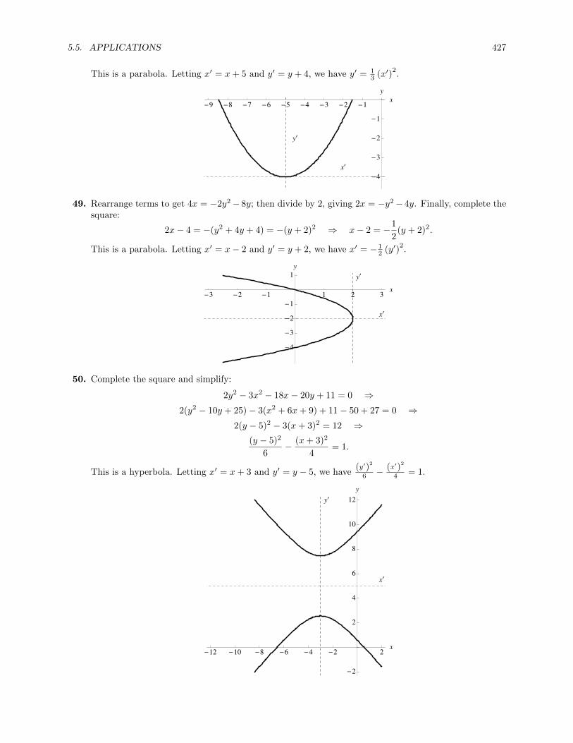
5.5. APPLICATIONS 427
This is a parabola. Letting x′ = x+ 5 and y′ = y + 4, we have y′ = 13 (x′)
2.
x¢
y¢
-9 -8 -7 -6 -5 -4 -3 -2 -1x
-4
-3
-2
-1
y
49. Rearrange terms to get 4x = −2y2− 8y; then divide by 2, giving 2x = −y2− 4y. Finally, complete thesquare:
2x− 4 = −(y2 + 4y + 4) = −(y + 2)2 ⇒ x− 2 = −1
2(y + 2)2.
This is a parabola. Letting x′ = x− 2 and y′ = y + 2, we have x′ = − 12 (y′)
2.
x¢
y¢
-3 -2 -1 1 2 3x
-4
-3
-2
-1
1
y
50. Complete the square and simplify:
2y2 − 3x2 − 18x− 20y + 11 = 0 ⇒2(y2 − 10y + 25)− 3(x2 + 6x+ 9) + 11− 50 + 27 = 0 ⇒
2(y − 5)2 − 3(x+ 3)2 = 12 ⇒(y − 5)2
6− (x+ 3)2
4= 1.
This is a hyperbola. Letting x′ = x+ 3 and y′ = y − 5, we have(y′)
2
6 − (x′)2
4 = 1.
x¢
y¢
-12 -10 -8 -6 -4 -2 2x
-2
2
4
6
8
10
12
y

428 CHAPTER 5. ORTHOGONALITY
51. The matrix of this form is
A =
[1 1
212 1
],
which has characteristic polynomial
(1− λ)2 − 1
4= λ2 − 2λ+
3
4=
(λ− 1
2
)(λ− 3
2
).
Therefore the associated diagonal matrix is
D =
[32 0
0 12
],
so that the equation becomes
xTAx = (x′)TDx′ =
3
2(x′)
2+
1
2(y′)
2= 6.
Dividing through by 6 to simplify gives
(x′)2
4+
(y′)2
12= 1,
which is an ellipse. To determine the rotation matrix Q, find unit eigenvectors corresponding to λ1 = 32
and λ2 = 12 by row-reduction to get
Q =
[1√2− 1√
21√2
1√2
].
Then
e1 → Qe1 =
[1√2
1√2
], e2 → Qe2 =
[− 1√
21√2
],
so that the axis rotation is through a 45◦ angle.
x¢
y¢
-3 -2 -1 1 2 3x
-3
-2
-1
1
2
3
y
52. The matrix of this form is
A =
[4 55 4
],

5.5. APPLICATIONS 429
which has characteristic polynomial
(4− λ)2 − 25 = λ2 − 8λ− 9 = (λ− 9)(λ+ 1).
Therefore the associated diagonal matrix is
D =
[9 00 −1
],
so that the equation becomes
xTAx = (x′)TDx′ = 9 (x′)
2 − (y′)2
= 9.
Dividing through by 9 to simplify gives
(x′)2 − (y′)
2
9= 1,
which is a hyperbola. To determine the rotation matrix Q, find unit eigenvectors corresponding toλ1 = 9 and λ2 = 1 by row-reduction to get
Q =
[1√2− 1√
21√2
1√2
].
Then
e1 → Qe1 =
[1√2
1√2
], e2 → Qe2 =
[− 1√
21√2
],
so that the axis rotation is through a 45◦ angle.
x¢
y¢
-3 -2 -1 1 2 3x
-3
-2
-1
1
2
3
y
53. The matrix of this form is
A =
[4 33 −4
],
which has characteristic polynomial
(4− λ)(−4− λ)− 9 = λ2 − 25 = (λ− 5)(λ+ 5)
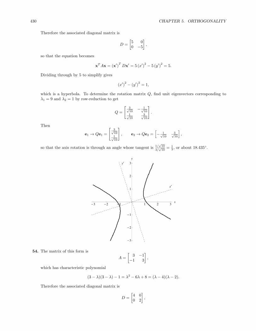
430 CHAPTER 5. ORTHOGONALITY
Therefore the associated diagonal matrix is
D =
[5 00 −5
],
so that the equation becomes
xTAx = (x′)TDx′ = 5 (x′)
2 − 5 (y′)2
= 5.
Dividing through by 5 to simplify gives
(x′)2 − (y′)
2= 1,
which is a hyperbola. To determine the rotation matrix Q, find unit eigenvectors corresponding toλ1 = 9 and λ2 = 1 by row-reduction to get
Q =
[3√10− 1√
101√10
3√10
].
Then
e1 → Qe1 =
[3√101√10
], e2 → Qe2 =
[− 1√
103√10
],
so that the axis rotation is through an angle whose tangent is 1/√
10
3/√
10= 1
3 , or about 18.435◦.
x¢
y¢
-3 -2 -1 1 2 3x
-3
-2
-1
1
2
3
y
54. The matrix of this form is
A =
[3 −1−1 3
],
which has characteristic polynomial
(3− λ)(3− λ)− 1 = λ2 − 6λ+ 8 = (λ− 4)(λ− 2).
Therefore the associated diagonal matrix is
D =
[4 00 2
],

5.5. APPLICATIONS 431
so that the equation becomes
xTAx = (x′)TDx′ = 4 (x′)
2+ 2 (y′)
2= 8.
Dividing through by 8 to simplify gives
(x′)2
2+
(y′)2
4= 1,
which is an ellipse. To determine the rotation matrix Q, find unit eigenvectors corresponding to λ1 = 4and λ2 = 2 by row-reduction to get
Q =
[1√2
1√2
− 1√2
1√2
].
Then
e1 → Qe1 =
[1√2
− 1√2
], e2 → Qe2 =
[1√2
1√2
],
so that the axis rotation is through a −45◦ angle.
x¢
y¢
-2 -1 1 2x
-2
-1
1
2
y
55. Writing the equation as xTAx +Bx + C = 0, we have
A =
[3 −2−2 3
], B =
[−28√
2 22√
2], C = 84.
A has characteristic polynomial
(3− λ)(3− λ)− 4 = λ2 − 6λ+ 5 = (λ− 5)(λ− 1).
Therefore the associated diagonal matrix is
D =
[5 00 1
].
To determine the rotation matrix Q, find unit eigenvectors corresponding to λ1 = 5 and λ2 = 1 byrow-reduction to get
Q =
[1√2
1√2
− 1√2
1√2
].

432 CHAPTER 5. ORTHOGONALITY
Thus
BQ =[−28√
2 22√
2] [ 1√
21√2
− 1√2
1√2
]=[−50 −6
],
so the equation becomes
5 (x′)2 − 50x′ + (y′)
2 − 6y′ = −84 ⇒
5(
(x′)2 − 10x′ + 25
)+(
(y′)2 − 6y′ + 9
)= −84 + 125 + 9 ⇒
5(x′ − 5)2 + (y′ − 3)2 = 50 ⇒(x′ − 5)2
10+
(y′ − 3)2
50= 1.
Letting x′′ = x′ − 5 and y′′ = y′ − 3 gives
(x′′)2
10+
(y′′)2
50= 1,
which is an ellipse.
56. Writing the equation as xTAx +Bx + C = 0, we have
A =
[6 −2−2 9
], B =
[−20 −10
], C = −5.
A has characteristic polynomial
(6− λ)(9− λ)− 4 = λ2 − 15λ+ 50 = (λ− 10)(λ− 15).
Therefore the associated diagonal matrix is
D =
[10 00 5
].
To determine the rotation matrix Q, find unit eigenvectors corresponding to λ1 = 10 and λ2 = 5 byrow-reduction to get
Q =
[− 1√
52√5
2√5
1√5
].
Thus
BQ =[−20 −10
] [− 1√5
2√5
2√5
1√5
]=[0 −10
√5],
so the equation becomes
10 (x′)2
+ 5 (y′)2 − 10
√5y′ = 5 ⇒
10 (x′)2
+ 5(
(y′)2 − 2
√5 y′ + 5
)= 5 + 25 ⇒
10 (x′)2
+ 5(y′ −
√5)2
= 30 ⇒
(x′)2
3+
(y′ −
√5)2
6= 1.
Letting x′′ = x′ and y′′ = y′ −√
5 gives
(x′′)2
3+
(y′′)2
6= 1,
which is an ellipse.
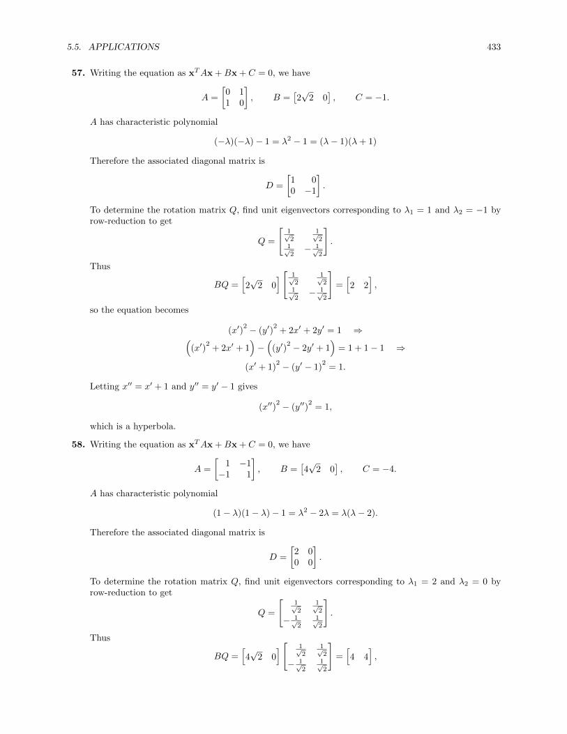
5.5. APPLICATIONS 433
57. Writing the equation as xTAx +Bx + C = 0, we have
A =
[0 11 0
], B =
[2√
2 0], C = −1.
A has characteristic polynomial
(−λ)(−λ)− 1 = λ2 − 1 = (λ− 1)(λ+ 1)
Therefore the associated diagonal matrix is
D =
[1 00 −1
].
To determine the rotation matrix Q, find unit eigenvectors corresponding to λ1 = 1 and λ2 = −1 byrow-reduction to get
Q =
[1√2
1√2
1√2− 1√
2
].
Thus
BQ =[2√
2 0] [ 1√
21√2
1√2− 1√
2
]=[2 2
],
so the equation becomes
(x′)2 − (y′)
2+ 2x′ + 2y′ = 1 ⇒(
(x′)2
+ 2x′ + 1)−(
(y′)2 − 2y′ + 1
)= 1 + 1− 1 ⇒
(x′ + 1)2 − (y′ − 1)
2= 1.
Letting x′′ = x′ + 1 and y′′ = y′ − 1 gives
(x′′)2 − (y′′)
2= 1,
which is a hyperbola.
58. Writing the equation as xTAx +Bx + C = 0, we have
A =
[1 −1−1 1
], B =
[4√
2 0], C = −4.
A has characteristic polynomial
(1− λ)(1− λ)− 1 = λ2 − 2λ = λ(λ− 2).
Therefore the associated diagonal matrix is
D =
[2 00 0
].
To determine the rotation matrix Q, find unit eigenvectors corresponding to λ1 = 2 and λ2 = 0 byrow-reduction to get
Q =
[1√2
1√2
− 1√2
1√2
].
Thus
BQ =[4√
2 0] [ 1√
21√2
− 1√2
1√2
]=[4 4
],

434 CHAPTER 5. ORTHOGONALITY
so the equation becomes
2 (x′)2
+ 4x′ + 4y′ = 4 ⇒
2y′ = − (x′)2 − 2x′ + 2 ⇒
2y′ − 1 = −(
(x′)2
+ 2x′ + 1)⇒
2
(y′ − 1
2
)= − (x′ + 1)
2 ⇒
y′ − 1
2= −1
2(x′ + 1)
2.
Letting x′′ = x′ + 1 and y′′ = y′ − 12 gives
y′′ = −1
2(x′′)
2,
which is a parabola.
59. x2 − y2 = (x+ y)(x− y) = 0 means that x = y or x = −y, so the graph of this degenerate conic is thepair of lines y = x and y = −x.
-2 -1 1 2
-2
-1
1
2
60. Rearranging terms gives x2 + 2y2 = −2, which has no solutions since the left-hand side is a sum of twosquares, so is always nonnegative. Therefore this is an imaginary conic.
61. The left-hand side is a sum of two squares, so it equals zero if and only if x = y = 0. The graph of thisdegenerate conic is the single point (0, 0).
-1. -0.5 0.5 1.
-1.
-0.5
0.5
1.

5.5. APPLICATIONS 435
62. x2 + 2xy + y2 = (x + y)2. Then (x + y)2 = 0 is satisfied only when x + y = 0, so the graph of thisdegenerate conic is the line y = −x.
-2 -1 1 2
-2
-1
1
2
63. Rearranging terms gives
x2 − 2xy + y2 = 2√
2(y − x), or (x− y)2 = 2√
2(y − x).
This is satisfied when y = x. If y 6= x, then we can divide through by y − x to get
y − x = 2√
2, or y = x+ 2√
2.
So the graph of this degenerate conic is the union of the lines y = x and y = x+ 2√
2.
-2 -1 1 2
-2
-1
1
2
3
4
64. Writing the equation as xTAx +Bx + C = 0, we have
A =
[2 11 2
], B =
[2√
2 −2√
2], C = 6.
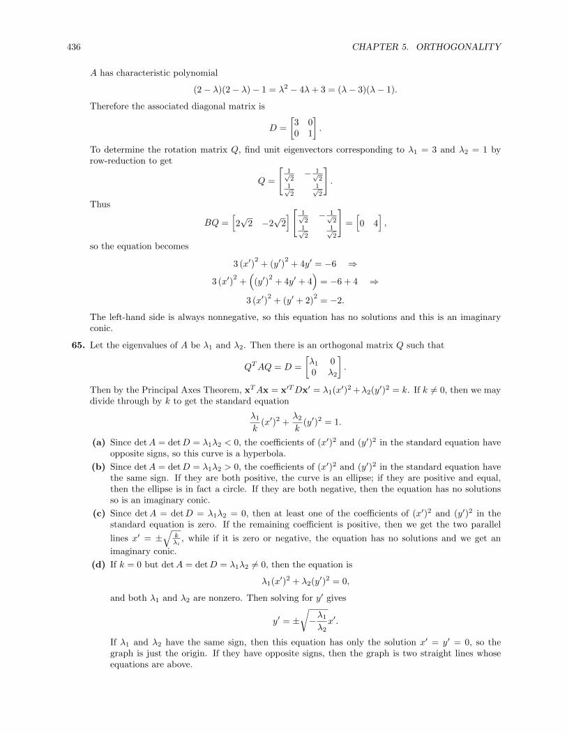
436 CHAPTER 5. ORTHOGONALITY
A has characteristic polynomial
(2− λ)(2− λ)− 1 = λ2 − 4λ+ 3 = (λ− 3)(λ− 1).
Therefore the associated diagonal matrix is
D =
[3 00 1
].
To determine the rotation matrix Q, find unit eigenvectors corresponding to λ1 = 3 and λ2 = 1 byrow-reduction to get
Q =
[1√2− 1√
21√2
1√2
].
Thus
BQ =[2√
2 −2√
2] [ 1√
2− 1√
21√2
1√2
]=[0 4
],
so the equation becomes
3 (x′)2
+ (y′)2
+ 4y′ = −6 ⇒
3 (x′)2
+(
(y′)2
+ 4y′ + 4)
= −6 + 4 ⇒
3 (x′)2
+ (y′ + 2)2
= −2.
The left-hand side is always nonnegative, so this equation has no solutions and this is an imaginaryconic.
65. Let the eigenvalues of A be λ1 and λ2. Then there is an orthogonal matrix Q such that
QTAQ = D =
[λ1 00 λ2
].
Then by the Principal Axes Theorem, xTAx = x′TDx′ = λ1(x′)2 +λ2(y′)2 = k. If k 6= 0, then we maydivide through by k to get the standard equation
λ1
k(x′)2 +
λ2
k(y′)2 = 1.
(a) Since detA = detD = λ1λ2 < 0, the coefficients of (x′)2 and (y′)2 in the standard equation haveopposite signs, so this curve is a hyperbola.
(b) Since detA = detD = λ1λ2 > 0, the coefficients of (x′)2 and (y′)2 in the standard equation havethe same sign. If they are both positive, the curve is an ellipse; if they are positive and equal,then the ellipse is in fact a circle. If they are both negative, then the equation has no solutionsso is an imaginary conic.
(c) Since detA = detD = λ1λ2 = 0, then at least one of the coefficients of (x′)2 and (y′)2 in thestandard equation is zero. If the remaining coefficient is positive, then we get the two parallel
lines x′ = ±√
kλi
, while if it is zero or negative, the equation has no solutions and we get an
imaginary conic.
(d) If k = 0 but detA = detD = λ1λ2 6= 0, then the equation is
λ1(x′)2 + λ2(y′)2 = 0,
and both λ1 and λ2 are nonzero. Then solving for y′ gives
y′ = ±√−λ1
λ2x′.
If λ1 and λ2 have the same sign, then this equation has only the solution x′ = y′ = 0, so thegraph is just the origin. If they have opposite signs, then the graph is two straight lines whoseequations are above.

5.5. APPLICATIONS 437
(e) If k = 0 and detA = detD = λ1λ2 = 0, then the equation is
λ1(x′)2 + λ2(y′)2 = 0,
and at least one of λ1 and λ2 is zero. If λ1 = 0, we get x′ = 0, so the graph is the y′-axis, astraight line. Similarly, if λ2 = 0, we get y′ = 0, so the graph is the x′-axis, also a straight line(if both λ1 and λ2 are zero, then A was the zero matrix to start, so it does not correspond to aquadratic form).
66. The matrix of this form is
A =
4 2 22 4 22 2 4
,which has characteristic polynomial
−λ3 + 12λ2 − 36λ+ 32 = −(λ− 2)2(λ− 8)
Therefore the associated diagonal matrix is
D =
8 0 00 2 00 0 2
,so that the equation becomes
xTAx = (x′)TDx′ = 8 (x′)
2+ 2 (y′)
2+ 2 (z′)
2= 8, or (x′)
2+
(y′)2
4+
(z′)2
4= 1.
This is an ellipsoid.
67. The matrix of this form is
A =
1 0 00 1 −20 −2 1
,which has characteristic polynomial
−λ3 + 3λ2 + λ− 3 = −(x+ 1)(x− 1)(x− 3)
Therefore the associated diagonal matrix is
D =
−1 0 00 1 00 0 3
,so that the equation becomes
xTAx = (x′)TDx′ = − (x′)
2+ (y′)
2+ 3 (z′)
2= 1,
which is a hyperboloid of one sheet.
68. The matrix of this form is
A =
−1 2 22 −1 22 2 −1
,which has characteristic polynomial
−λ3 − 3λ2 + 9λ+ 27 = −(x+ 3)2(x− 3)
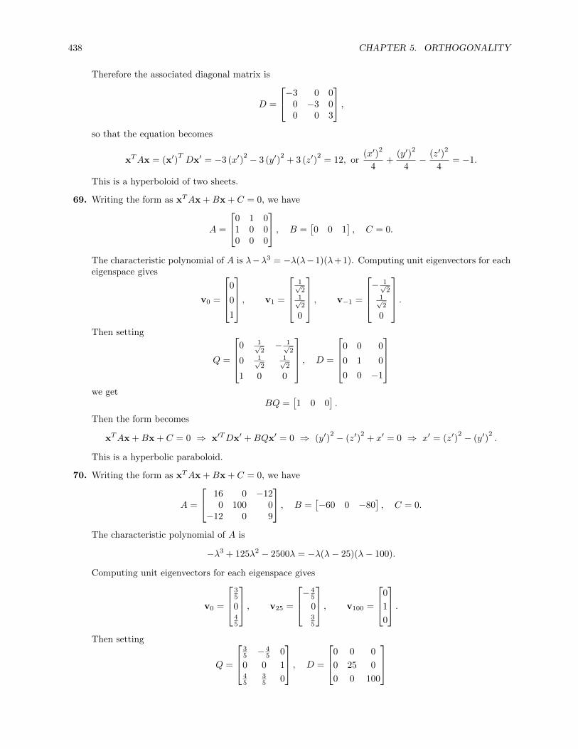
438 CHAPTER 5. ORTHOGONALITY
Therefore the associated diagonal matrix is
D =
−3 0 00 −3 00 0 3
,so that the equation becomes
xTAx = (x′)TDx′ = −3 (x′)
2 − 3 (y′)2
+ 3 (z′)2
= 12, or(x′)
2
4+
(y′)2
4− (z′)
2
4= −1.
This is a hyperboloid of two sheets.
69. Writing the form as xTAx +Bx + C = 0, we have
A =
0 1 01 0 00 0 0
, B =[0 0 1
], C = 0.
The characteristic polynomial of A is λ−λ3 = −λ(λ−1)(λ+ 1). Computing unit eigenvectors for eacheigenspace gives
v0 =
0
0
1
, v1 =
1√2
1√2
0
, v−1 =
− 1√
21√2
0
.Then setting
Q =
0 1√
2− 1√
2
0 1√2
1√2
1 0 0
, D =
0 0 0
0 1 0
0 0 −1
we get
BQ =[1 0 0
].
Then the form becomes
xTAx +Bx + C = 0 ⇒ x′TDx′ +BQx′ = 0 ⇒ (y′)2 − (z′)
2+ x′ = 0 ⇒ x′ = (z′)
2 − (y′)2.
This is a hyperbolic paraboloid.
70. Writing the form as xTAx +Bx + C = 0, we have
A =
16 0 −120 100 0
−12 0 9
, B =[−60 0 −80
], C = 0.
The characteristic polynomial of A is
−λ3 + 125λ2 − 2500λ = −λ(λ− 25)(λ− 100).
Computing unit eigenvectors for each eigenspace gives
v0 =
35
045
, v25 =
−45
035
, v100 =
0
1
0
.Then setting
Q =
35 − 4
5 0
0 0 145
35 0
, D =
0 0 0
0 25 0
0 0 100

5.5. APPLICATIONS 439
we get
BQ =[−100 0 0
].
Then the form becomes
xTAx+Bx+C = 0 ⇒ x′TDx′+BQx′ = 0 ⇒ 25 (y′)2
+100 (z′)2−100x′ = 0 ⇒ x′ =
(y′)2
4+(z′)
2.
This is an elliptic paraboloid.
71. Writing the form as xTAx +Bx + C = 0, we have
A =
1 2 −12 1 1−1 1 −2
, B =[−1 1 1
], C = 0.
The characteristic polynomial of A is
−λ3 + 9λ = −λ(λ− 3)(λ+ 3).
Computing unit eigenvectors for each eigenspace gives
v0 =
− 1√
31√3
1√3
, v3 =
1√2
1√2
0
, v−3 =
1√6
− 1√6
2√6
.Then setting
Q =
− 1√
31√2
1√6
1√3
1√2− 1√
61√3
0 2√6
, D =
0 0 0
0 3 0
0 0 −3
we get
BQ =[√
3 0 0].
Then the form becomes
xTAx+Bx+C = 0 ⇒ x′TDx′+BQx′ = 0 ⇒ 3 (y′)2− 3 (z′)
2+√
3x′ = 0 ⇒ x′ =(y′)
2
1/√
3− (z′)
2
1/√
3
This is a hyperbolic paraboloid.
72. Writing the form as xTAx +Bx = 15, we have
A =
10 0 −200 25 0
−20 0 10
, B =[20√
2 50 20√
2].
The characteristic polynomial of A is
−λ3 + 45λ2 − 200λ− 7500 = −(λ+ 10)(λ− 25)(λ− 30).
Computing unit eigenvectors for each eigenspace gives
v−10 =
1√2
01√2
, v25 =
0
1
0
, v30 =
− 1√
2
01√2
.

440 CHAPTER 5. ORTHOGONALITY
Then setting
Q =
1√2
0 − 1√2
0 1 01√2
0 1√2
, D =
−10 0 0
0 25 0
0 0 30
we get
BQ =[40 50 0
].
Then the form becomes
xTAx +Bx = 15 ⇒x′TDx′ +BQx′ = 15 ⇒
−10 (x′)2
+ 25 (y′)2
+ 30 (z′)2
+ 40x′ + 50y′ = 15 ⇒
−10(
(x′)2
+ 4x′)
+ 25(
(y′)2
+ 2y′)
+ 30 (z′)2
= 15⇒
−10 (x′ + 2)2
+ 25 (y′ + 1)2
+ 30 (z′)2
= 0⇒
(x′ + 2)2
=(y′ + 1)
2
2/5+
(z′)2
1/3.
Letting x′′ = x′ + 2, y′′ = y′ + 1, z′′ = z′ gives
(x′′)2
=(y′′)
2
2/5+
(z′′)2
1/3.
This is an elliptic cone.
73. Writing the form as xTAx +Bx = 6, we have
A =
11 1 41 11 −44 −4 14
, B =[−12 12 12
].
The characteristic polynomial of A is
−λ3 + 36λ2 − 396λ+ 1296 = −(λ− 6)(λ− 12)(λ− 18).
Computing unit eigenvectors for each eigenspace gives
v6 =
− 1√
31√3
1√3
, v12 =
1√2
1√2
0
, v18 =
1√6
− 1√6
2√6
.Then setting
Q =
− 1√
31√2
1√6
1√3
1√2− 1√
61√3
0 2√6
, D =
6 0 0
0 12 0
0 0 18
we get
BQ =[12√
3 0 0].

5.5. APPLICATIONS 441
Then the form becomes
xTAx +Bx = 6 ⇒x′TDx′ +BQx′ = 6 ⇒
6 (x′)2
+ 12 (y′)2
+ 18 (z′)2
+ 12√
3x′6 ⇒
6(
(x′)2
+ 2√
3x′)
+ 12 (y′)2
+ 18 (z′)2
= 6⇒
6(
(x′)2
+ 2√
3x′ + 3)
+ 12 (y′)2
+ 18 (z′)2
= 24⇒(x′ +
√3)2
4+
(y′)2
2+
(z′)2
4/3= 1.
Letting x′′ = x′ +√
3, y′′ = y′, z′′ = z′ gives
(x′′)2
4+
(y′′)2
2+
(z′′)2
4/3= 1.
This is an ellipsoid.
74. The strategy is to reduce the problem to one in which we can apply part (b) of Exercise 65. Using the
hint, let v be an eigenvector corresponding to λ = a−bi, and let P =[Rev Imv
]. Set B =
(PPT
)−1.
Now, B is a real matrix; it is also symmetric since
BT =((PPT
)−1)T
=((PPT
)T)−1
=((PT)TPT)−1
=(PPT
)−1= B.
Also,
detB = det((PPT
)−1)
=1
det (PPT )=
1
detP detPT=
1
(detP )2 > 0.
Thus Exercise 65(b) applies to B, so that xTBx = k is an ellipse if both eigenvalues of B are positive(since k > 0). But by Exercise 29 in this section, B−1 is positive definite, so that B is as well (Exercise31(d)), and therefore has positive eigenvalues. Hence the trajectories of xTB are ellipses.
Next, let
C =
[a −bb a
],
so that by Theorem 4.43, A = PCP−1. Note that
CTC =
[a b−b a
] [a −bb a
]=
[a2 + b2 ab− abab− ab a2 + b2
]=
[|λ|2 00 |λ|
]=
[1 00 1
]= I.
Now,
(Ax)TB(Ax) = xTAT(PPT
)−1(Ax)
= xT(PCP−1
)T (PT)−1
P−1PCP−1x
= xT(P−1
)TCTPT
(PT)−1
CP−1x
= xT(PT)−1
CTCP−1x
= xT(PT)−1
P−1x
= xT(PPT
)−1x
= xTBx.
Thus the quadratics xTBx = k and (Ax)TB(Ax) = k are the same, so that the trajectories of Ax areellipses as well.
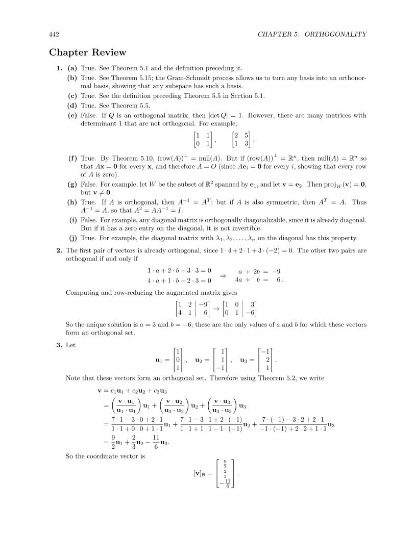
442 CHAPTER 5. ORTHOGONALITY
Chapter Review
1. (a) True. See Theorem 5.1 and the definition preceding it.
(b) True. See Theorem 5.15; the Gram-Schmidt process allows us to turn any basis into an orthonor-mal basis, showing that any subspace has such a basis.
(c) True. See the definition preceding Theorem 5.5 in Section 5.1.
(d) True. See Theorem 5.5.
(e) False. If Q is an orthogonal matrix, then |detQ| = 1. However, there are many matrices withdeterminant 1 that are not orthogonal. For example,[
1 10 1
],
[2 51 3
].
(f) True. By Theorem 5.10, (row(A))⊥
= null(A). But if (row(A))⊥
= Rn, then null(A) = Rn sothat Ax = 0 for every x, and therefore A = O (since Aei = 0 for every i, showing that every rowof A is zero).
(g) False. For example, let W be the subset of R2 spanned by e1, and let v = e2. Then projW (v) = 0,but v 6= 0.
(h) True. If A is orthogonal, then A−1 = AT ; but if A is also symmetric, then AT = A. ThusA−1 = A, so that A2 = AA−1 = I.
(i) False. For example, any diagonal matrix is orthogonally diagonalizable, since it is already diagonal.But if it has a zero entry on the diagonal, it is not invertible.
(j) True. For example, the diagonal matrix with λ1, λ2, . . . , λn on the diagonal has this property.
2. The first pair of vectors is already orthogonal, since 1 · 4 + 2 · 1 + 3 · (−2) = 0. The other two pairs areorthogonal if and only if
1 · a+ 2 · b+ 3 · 3 = 0
4 · a+ 1 · b− 2 · 3 = 0⇒ a + 2b = −9
4a + b = 6 .
Computing and row-reducing the augmented matrix gives[1 2 −94 1 6
]→[1 0 30 1 −6
]So the unique solution is a = 3 and b = −6; these are the only values of a and b for which these vectorsform an orthogonal set.
3. Let
u1 =
101
, u2 =
11−1
, u3 =
−121
.Note that these vectors form an orthogonal set. Therefore using Theorem 5.2, we write
v = c1u1 + c2u2 + c3u3
=
(v · u1
u1 · u1
)u1 +
(v · u2
u2 · u2
)u2 +
(v · u3
u3 · u3
)u3
=7 · 1− 3 · 0 + 2 · 11 · 1 + 0 · 0 + 1 · 1
u1 +7 · 1− 3 · 1 + 2 · (−1)
1 · 1 + 1 · 1− 1 · (−1)u2 +
7 · (−1)− 3 · 2 + 2 · 1−1 · (−1) + 2 · 2 + 1 · 1
u3
=9
2u1 +
2
3u2 −
11
6u3.
So the coordinate vector is
[v]B =
9223
− 116
.

Chapter Review 443
4. We first find v2. Since v1 and v2 =
[xy
]are orthogonal, we have
3
5x+
4
5y = 0, or x = −4
3y.
But also v2 is a unit vector, so that x2 + y2 = 169 y
2 + y2 = 259 y
2 = 1. Therefore y = ± 35 and x = ∓ 4
5 .
• If v2 =[− 4
535
], then
v = −3v1 +1
2v2 = −3
[3545
]+
1
2
[− 4
535
]=
[− 11
5
− 2110
].
• If v2 =[
45 − 3
5
], then
v = −3v1 +1
2v2 = −3
[3545
]+
1
2
[45
− 35
]=
[− 7
5
− 2710
].
5. Using Theorem 5.5, we show that the matrix is orthogonal by showing that that QQT = I:
QQT =
67
27
37
− 1√5
0 2√5
47√
5− 15
7√
52
7√
5
67 − 1√
54
7√
527 0 − 15
7√
537
2√5
27√
5
=
1 0 0
0 1 0
0 0 1
= I.
6. Let Q be the given matrix. If Q is to be orthogonal, then by Theorem 5.5, we must have
QQT =
[12 a
b c
][12 b
a c
]=
[14 + a2 1
2b+ ac12b+ ac b2 + c2
]=
[1 0
0 1
].
Therefore we must have
a2 +1
4= 1, ac+
1
2b = 0, b2 + c2 = 1.
The first equation gives a = ±√
32 . Substituting this into the second equation gives
±√
3
2c+
1
2b = 0, ⇒ b = ∓
√3 c ⇒ b2 = 3c2.
But b2 + c2 = 1 and b2 = 3c2 means that 4c2 = 1, so that c = ± 12 . So there are two possibilities:
• If a =√
32 , then b = −
√3 c, so we get the two matrices[
12
√3
2
−√
32
12
],
[12
√3
2√3
2 − 12
].
• If a = −√
32 , then b =
√3 c, so we get the two matrices[
12 −
√3
2√3
212
],
[12 −
√3
2
−√
32 − 1
2
].
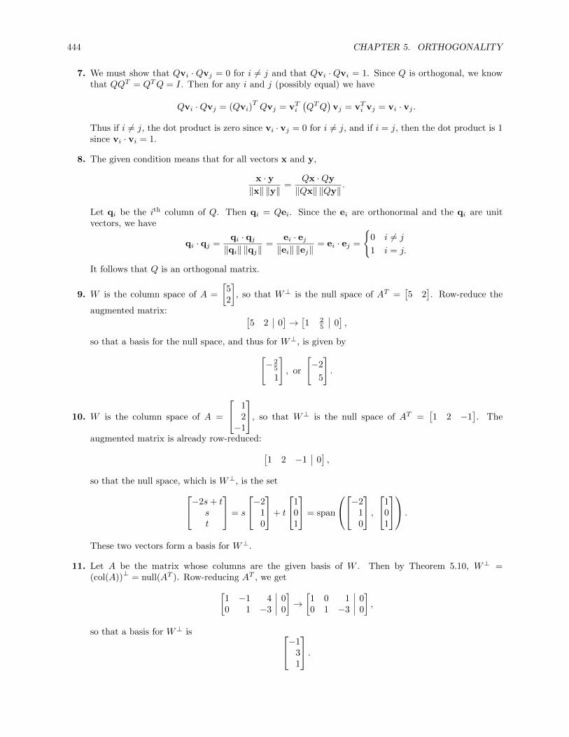
444 CHAPTER 5. ORTHOGONALITY
7. We must show that Qvi ·Qvj = 0 for i 6= j and that Qvi ·Qvi = 1. Since Q is orthogonal, we knowthat QQT = QTQ = I. Then for any i and j (possibly equal) we have
Qvi ·Qvj = (Qvi)TQvj = vTi
(QTQ
)vj = vTi vj = vi · vj .
Thus if i 6= j, the dot product is zero since vi · vj = 0 for i 6= j, and if i = j, then the dot product is 1since vi · vi = 1.
8. The given condition means that for all vectors x and y,
x · y‖x‖ ‖y‖
=Qx ·Qy
‖Qx‖ ‖Qy‖.
Let qi be the ith column of Q. Then qi = Qei. Since the ei are orthonormal and the qi are unitvectors, we have
qi · qj =qi · qj‖qi‖ ‖qj‖
=ei · ej‖ei‖ ‖ej‖
= ei · ej =
{0 i 6= j
1 i = j.
It follows that Q is an orthogonal matrix.
9. W is the column space of A =
[52
], so that W⊥ is the null space of AT =
[5 2
]. Row-reduce the
augmented matrix: [5 2 0
]→[1 2
5 0],
so that a basis for the null space, and thus for W⊥, is given by[− 2
5
1
], or
[−2
5
].
10. W is the column space of A =
12−1
, so that W⊥ is the null space of AT =[1 2 −1
]. The
augmented matrix is already row-reduced: [1 2 −1 0
],
so that the null space, which is W⊥, is the set−2s+ tst
= s
−210
+ t
101
= span
−210
,1
01
.
These two vectors form a basis for W⊥.
11. Let A be the matrix whose columns are the given basis of W . Then by Theorem 5.10, W⊥ =(col(A))
⊥= null(AT ). Row-reducing AT , we get[
1 −1 4 00 1 −3 0
]→[1 0 1 00 1 −3 0
],
so that a basis for W⊥ is −131
.
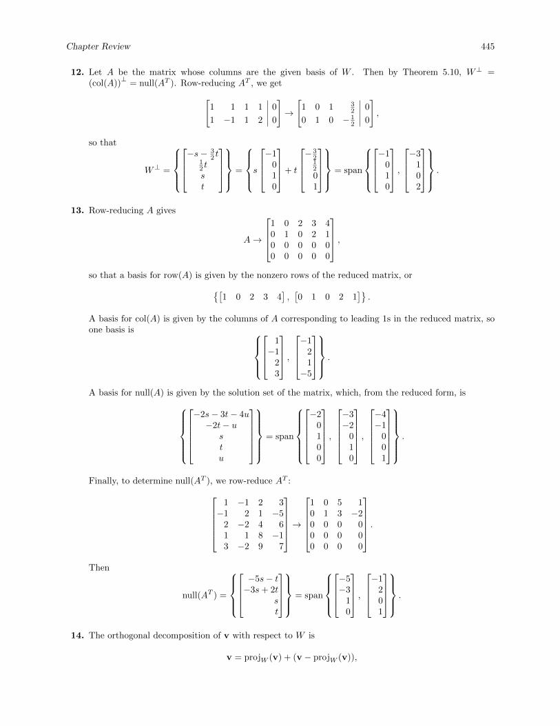
Chapter Review 445
12. Let A be the matrix whose columns are the given basis of W . Then by Theorem 5.10, W⊥ =(col(A))
⊥= null(AT ). Row-reducing AT , we get[
1 1 1 1 0
1 −1 1 2 0
]→
[1 0 1 3
2 0
0 1 0 − 12 0
],
so that
W⊥ =
−s− 3
2 t12 tst
=
s−1
010
+ t
− 3
21201
= span
−1
010
,−3
102
.
13. Row-reducing A gives
A→
1 0 2 3 40 1 0 2 10 0 0 0 00 0 0 0 0
,so that a basis for row(A) is given by the nonzero rows of the reduced matrix, or{[
1 0 2 3 4],[0 1 0 2 1
]}.
A basis for col(A) is given by the columns of A corresponding to leading 1s in the reduced matrix, soone basis is
1−1
23
,−1
21−5
.
A basis for null(A) is given by the solution set of the matrix, which, from the reduced form, is
−2s− 3t− 4u−2t− u
stu
= span
−2
0100
,−3−2
010
,−4−1
001
.
Finally, to determine null(AT ), we row-reduce AT :1 −1 2 3−1 2 1 −5
2 −2 4 61 1 8 −13 −2 9 7
→
1 0 5 10 1 3 −20 0 0 00 0 0 00 0 0 0
.
Then
null(AT ) =
−5s− t−3s+ 2t
st
= span
−5−3
10
,−1
201
.
14. The orthogonal decomposition of v with respect to W is
v = projW (v) + (v − projW (v)),

446 CHAPTER 5. ORTHOGONALITY
so we must find projW (v). Let the three given vectors in W be w1, w2, and w3. Then
projW (v) =
(w1 · vw1 ·w1
)w1 +
(w2 · vw2 ·w2
)w2 +
(w3 · vw3 ·w3
)w3
=0 · 1 + 1 · 0 + 1 · (−1) + 1 · 2
0 · 0 + 1 · 1 + 1 · 1 + 1 · 1
0111
+1 · 1 + 0 · 0 + 1 · (−1)− 1 · 21 · 1 + 0 · 0 + 1 · 1− 1 · (−1)
101−1
+3 · 1 + 1 · 0− 2 · (−1) + 1 · 23 · 3 + 1 · 1− 2 · (−2) + 1 · 1
31−2
1
=1
3
0111
− 2
3
101−1
+7
15
31−2
1
=
111545
− 19152215
.Then
v − projW (v) =
1
0
−1
2
−
111545
− 19152215
=
415
− 45415815
.15. (a) Using Gram-Schmidt, we get
v1 = x1 =
1111
v2 = x2 − projv1(x2)v1 =
1110
−−1 · 1 + 1 · 1 + 1 · 1 + 1 · 01 · 1 + 1 · 1 + 1 · 1 + 1 · 1
1111
=
1110
− 3
4
1111
=
141414
− 34
v3 = x3 − projv1
(x3)v1 − projv2(x3)v2
=
0111
− 1 · 0 + 1 · 1 + 1 · 1 + 1 · 11 · 1 + 1 · 1 + 1 · 1 + 1 · 1
v1 −14 · 0 + 1
4 · 1 + 14 · 1−
34 · 1
116 + 1
16 + 116 + 9
16
v2
=
0111
− 3
4
1111
+1
3
141414
− 34
=
− 2
31313
0
.

Chapter Review 447
(b) To find a QR factorization, we normalize the vectors from (a) and use those as the column vectorsof Q. Then we set R = QTA. Normalizing v1, v2, and v3 yields
q1 =v1
‖v1‖=
1
2
1
1
1
1
=
12121212
q2 =v2
‖v2‖=
2√
3
3
141414
− 34
=
√
36√3
6√3
6
−√
32
q3 =v3
‖v3‖=
√6
2
− 2
31313
0
=
−√
63√6
6√6
6
0
.
Then
Q =
12
√3
6 −√
63
12
√3
6
√6
612
√3
6
√6
612 −
√3
2 0
,
and
R = QTA =
12
12
12
12√
36
√3
6
√3
6 −√
32
−√
63
√6
6
√6
6 0
1 1 0
1 1 1
1 1 1
1 0 1
=
2 3
232
0√
32 −
√3
6
0 0√
63
.
Then A = QR is a QR factorization of A.
16. Note that the two given vectors,
v1 =
1022
and v2 =
011−1
,
are indeed orthogonal. We extend these to a basis by adding e3 and e4. We can verify that this is abasis by computing the determinant of the matrix whose column vectors are the vi; this determinantis 1, so the matrix is invertible and therefore the vectors are linearly independent, so they do in fact

448 CHAPTER 5. ORTHOGONALITY
form a basis for R4. We apply Gram-Schmidt to v3 and v4:
v3 = x3 − projv1(x3)v1 − projv2
(x3)v2
=
0
0
1
0
− 0 · 1 + 0 · 0 + 1 · 2 + 0 · 212 + 02 + 22 + 22
v1 −0 · 0 + 0 · 1 + 1 · 1 + 0 · (−1)
02 + 12 + 12 + (−1)2v2
=
0
0
1
0
− 2
9
1
0
2
2
− 1
3
0
1
1
−1
=
− 2
9
− 1329
− 19
v4 = x4 − projv1
(x4)v1 − projv2(x4)v2 − projv3
(x4)v3
=
0
0
0
1
− 0 · 1 + 0 · 0 + 0 · 2 + 1 · 212 + 02 + 22 + 22
v1 −0 · 0 + 0 · 1 + 0 · 1 + 0 · (−1)
02 + 12 + 12 + (−1)2v2
−0 ·(− 2
9
)+ 0 ·
(− 1
3
)+ 0 · 2
9 + 1 ·(− 1
9
)481 + 1
9 + 481 + 1
81
v3
=
0
0
0
1
− 2
9
1
0
2
2
+1
3
0
1
1
−1
+1
2
− 2
9
− 1329
− 19
=
− 1
316
016
.
17. If x1 + x2 + x3 + x4 = 0, then x4 = −x1 − x2 − x3, so that a basis for W is given by
B =
x1 =
100−1
, x2 =
010−1
, x3 =
001−1
.
Then using Gram-Schmidt,
v1 = x1 =
1
0
0
−1
v2 = x2 − projv1(x2)v1 =
0
1
0
−1
−−1 · 0 + 0 · 1 + 0 · 0− 1 · (−1)
12 + 02 + 02 + (−1)2
1
0
0
−1
=
0
1
0
−1
− 1
2
1
0
0
−1
=
− 1
2
1
0
− 12
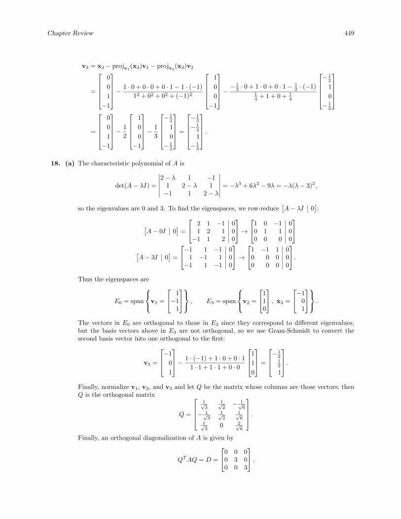
Chapter Review 449
v3 = x3 − projv1(x3)v1 − projv2
(x3)v2
=
0
0
1
−1
− 1 · 0 + 0 · 0 + 0 · 1− 1 · (−1)
12 + 02 + 02 + (−1)2
1
0
0
−1
− − 12 · 0 + 1 · 0 + 0 · 1− 1
2 · (−1)14 + 1 + 0 + 1
4
− 1
2
1
0
− 12
=
0
0
1
−1
− 1
2
1
0
0
−1
− 1
3
− 1
2
1
0
− 12
=
− 1
3
− 13
1
− 13
.
18. (a) The characteristic polynomial of A is
det(A− λI) =
∣∣∣∣∣∣2− λ 1 −1
1 2− λ 1−1 1 2− λ
∣∣∣∣∣∣ = −λ3 + 6λ2 − 9λ = −λ(λ− 3)2,
so the eigenvalues are 0 and 3. To find the eigenspaces, we row-reduce[A− λI 0
]:
[A− 0I 0
]=
2 1 −1 01 2 1 0−1 1 2 0
→1 0 −1 0
0 1 1 00 0 0 0
[A− 3I 0
]=
−1 1 −1 01 −1 1 0−1 1 −1 0
→1 −1 1 0
0 0 0 00 0 0 0
.Thus the eigenspaces are
E0 = span
v1 =
1−1
1
, E3 = span
v2 =
110
, x3 =
−101
.
The vectors in E0 are orthogonal to those in E3 since they correspond to different eigenvalues,but the basis vectors above in E3 are not orthogonal, so we use Gram-Schmidt to convert thesecond basis vector into one orthogonal to the first:
v3 =
−1
0
1
− 1 · (−1) + 1 · 0 + 0 · 11 · 1 + 1 · 1 + 0 · 0
1
1
0
=
−1212
1
.Finally, normalize v1, v2, and v3 and let Q be the matrix whose columns are those vectors; thenQ is the orthogonal matrix
Q =
1√3
1√2− 1√
6
− 1√3
1√2
1√6
1√3
0 2√6
.Finally, an orthogonal diagonalization of A is given by
QTAQ = D =
0 0 00 3 00 0 3
.

450 CHAPTER 5. ORTHOGONALITY
(b) From part (a), we have λ1 = 0 and λ2 = λ3 = 3, with
q1 =
1√3
− 1√3
1√3
, q2 =
1√2
1√2
0
, q3 =
− 1√
61√6
2√6
.The spectral decomposition of A is
A = λ1q1qT1 + λ2q2q
T2 + λ3q3q
T3
= 3q2qT2 + 3q3q
T3
= 3
1√2
1√2
0
[
1√2
1√2
0
]+ 3
− 1√
61√6
2√6
[− 1√6
1√6
2√6
]
= 3
12
12 0
12
12 0
0 0 0
+ 3
16 − 1
6 − 13
− 16
16
13
− 13
13
23
.19. See Example 5.20, or Exercises 23 and 24 in Section 5.4. The basis vector for E−2, which we name
v3 =
1−1
0
, is orthogonal to the other two since they correspond to different eigenvalues. However,
we must orthogonalize the basis for E0 using Gram-Schmidt:
v1 =
1
1
0
, v2 =
1
1
1
− 1 · 1 + 1 · 1 + 1 · 012 + 12 + 02
1
1
0
=
0
0
1
.Now v1, v2, and v3 are mutually orthogonal, with norms
√2,√
2, and 1 respectively. Let Q be thematrix whose columns are q1 = v1
‖v1‖ , q2 = v2
‖v2‖ , and q3 = v3
‖v3‖ ; then the desired matrix is
Q
1 0 0
0 1 0
0 0 −2
Q−1 = Q
1 0 0
0 1 0
0 0 −2
QT
=
1√2
0 1√2
− 1√2
0 1√2
0 1 0
1 0 0
0 1 0
0 0 −2
1√2− 1√
20
0 0 11√2
1√2
0
=
− 1
2 − 32 0
− 32 − 1
2 0
0 0 1
.20. viv
Ti is symmetric since (
vivTi
)T=(vTi)T
vTi = vTi vi,
so it is equal to its own transpose. Since a scalar times a symmetric matrix is a symmetric matrix, andthe sum of symmetric matrices is symmetric, it follows that A is symmetric. Next,
Avj =
(n∑i=1
civivTi
)vj =
n∑i=1
civi(vTi vj
)=
n∑i=1
civi (vi · vj) = cjvj
since {vi} is a set of orthonormal vectors. This shows that each cj is an eigenvalue for A withcorresponding eigenvector vj . Since there are n of them, these are all the eigenvalues and eigenvectors.

Chapter 6
Vector Spaces
6.1 Vector Spaces and Subspaces
1. Let V =
{[xx
]}. V is the set of all vectors in R2 whose first and second components are the same.
We verify all ten axioms of a vector space:
1. If
[xx
],
[yy
]∈ V then
[xx
]+
[yy
]=
[x+ yx+ y
]∈ V since its first and second components are the same.
2.
[xx
]+
[yy
]=
[x+ yx+ y
]=
[y + xy + x
]=
[yy
]+
[xx
].
3.
([xx
]+
[yy
])+
[zz
]=
[x+ yx+ y
]+
[zz
]=
[x+ y + zx+ y + z
]=
[xx
]+
[y + zy + z
]=
[xx
]+
([yy
]+
[zz
]).
4.
[00
]∈ V , and
[xx
]+
[00
]=
[x+ 0x+ 0
]=
[xx
]∈ V .
5. If
[xx
]∈ V , then
[−x−x
]∈ V , and
[xx
]+
[−x−x
]=
[x− xx− x
]=
[00
].
6. If
[xx
]∈ V , then c
[xx
]=
[cxcx
]∈ V since its first and second components are the same.
7. c
([xx
]+
[yy
])= c
[x+ yx+ y
]=
[c(x+ y)c(x+ y)
]=
[c(y + x)c(y + x)
]= c
[y + xy + x
]= c
([yy
]+
[xx
]).
8. (c+ d)
[xx
]=
[(c+ d)x(c+ d)x
]=
[cx+ dxcx+ dx
]=
[cxcx
]+
[dxdx
]= c
[xx
]+ d
[xx
].
9. c
(d
[xx
])= c
[dxdx
]=
[c(dx)c(dx)
]=
[(cd)x(cd)x
]= (cd)
[xx
].
10. 1
[xx
]=
[1x1x
]=
[xx
].
2. V =
{[xy
]: x, y ≥ 0
}fails to satisfy Axioms 5 and 6, so it is not a vector space:
5. If
[xy
]6=[00
]∈ V , choose c < 0; then c
[xy
]=
[cxcy
]/∈ V since at least one of cx and cy is negative.
6. If
[xx
]6=[00
]∈ V , then
[−x−x
]/∈ V since −x < 0.
451

452 CHAPTER 6. VECTOR SPACES
3. V =
{[xy
]: xy ≥ 0
}fails to satisfy Axiom 1, so it is not a vector space:
1. Choose x 6= y with xy ≥ 0. Then
[xy
]and
[−y−x
]are both in V , but
[xy
]+
[−y−x
]=
[x− yy − x
]=
[x− y−(x− y)
]/∈ V
since (x− y)(−(x− y)) = −(x− y)2 < 0 because x 6= y.
4. V =
{[xy
]: x ≥ y
}fails to satisfy Axioms 5 and 6, so it is not a vector space:
5. If
[xy
]∈ V and x 6= y, then x > y, so that −x < −y. Therefore
[−x−y
]/∈ V .
6. Again let
[xy
]∈ V and x 6= y, and choose c = −1. Then
[cxcy
]=
[−x−y
]/∈ V as above.
.
5. R2 with the given scalar multiplication fails to satisfy Axiom 8, so it is not a vector space:
8. Choose
[xy
]∈ R2 with y 6= 0, and let c and d be nonzero scalars. Then
(c+ d)
[xy
]=
[(c+ d)x
y
]=
[cx+ dx
y
], while c
[xy
]+ d
[xy
]=
[cxy
]+
[dxy
]=
[cx+ dx
2y
].
These two are unequal since we chose y 6= 0.
6. R2 with the given addition fails to satisfy Axiom 7, so it is not a vector space:
8. Choose
[x1
y1
],
[x2
y2
]∈ R2 and let c be a scalar not equal 1. Then
c
([x1
y1
]+
[x2
y2
])= c
[x1 + x2 + 1y1 + y2 + 1
]=
[cx1 + cx2 + ccy1 + cy2 + c
]c
[x1
y1
]+ c
[x2
y2
]=
[cx1
cy1
]+
[cx2
cy2
]=
[cx1 + cx2 + 1cy1 + cy2 + 1
].
These two are unequal since we chose c 6= 1.
7. All axioms apply, so that this set is a vector space. Let x, y, and z by positive real numbers, so thatx, y, z ∈ V , and c and d be any real numbers. Then
1. x⊕ y = xy > 0, so that x⊕ y ∈ V .
2. x⊕ y = xy = yx = y ⊕ x.
3. (x⊕ y)⊕ z = (xy)⊕ z = (xy)z = x(yz) = x⊕ (yz) = x⊕ (y ⊕ z).4. 0 = 1, since x⊕ 0 = x1 = 1x = 0⊕ x = x.
5. −x is the positive real number 1x , since x⊕ (−x) = x · 1
x = 1 = 0.
6. c� x = xc > 0, so that c� x ∈ V .
7. c� (x⊕ y) = (xy)c = xcyc = xc ⊕ yc = (c� x)⊕ (c� y).
8. (c+ d)� x = xc+d = xcxd = xc ⊕ xd = (c� x)⊕ (c� y).
9. c� (d� x) = c� xd =(xd)c
= xcd = (xc)d
= d� xc = d� (c� x).
10. 1� x = xx = x.
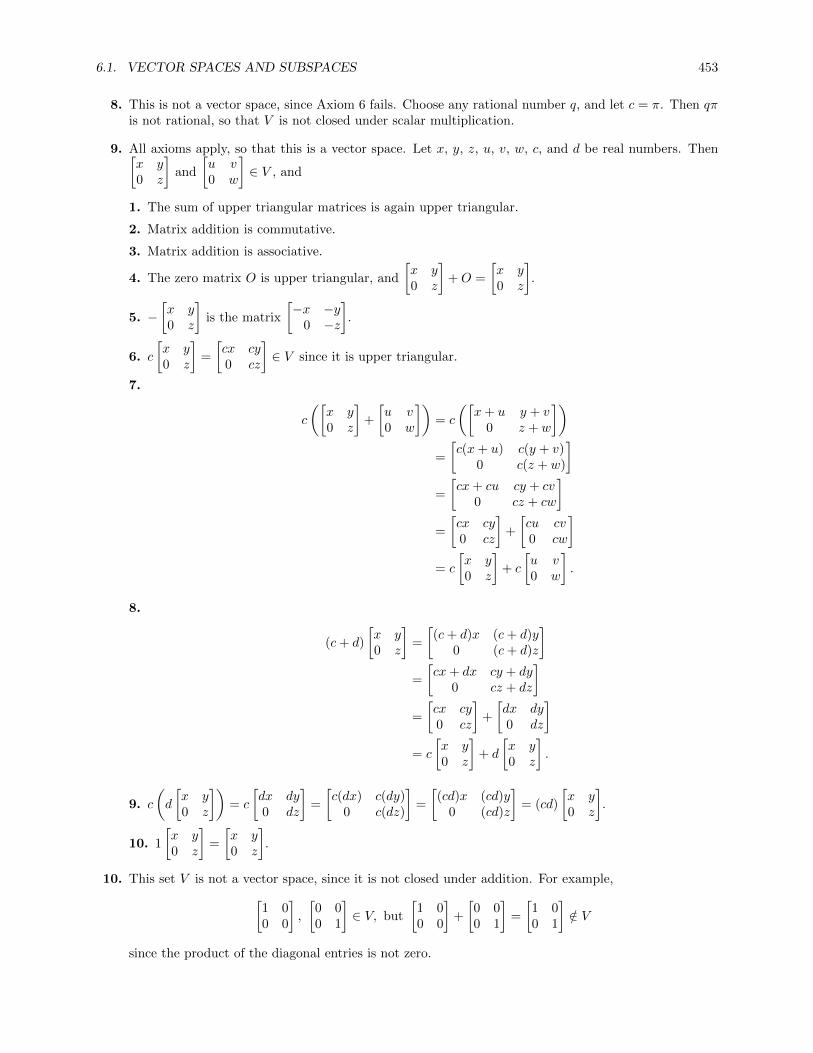
6.1. VECTOR SPACES AND SUBSPACES 453
8. This is not a vector space, since Axiom 6 fails. Choose any rational number q, and let c = π. Then qπis not rational, so that V is not closed under scalar multiplication.
9. All axioms apply, so that this is a vector space. Let x, y, z, u, v, w, c, and d be real numbers. Then[x y0 z
]and
[u v0 w
]∈ V , and
1. The sum of upper triangular matrices is again upper triangular.
2. Matrix addition is commutative.
3. Matrix addition is associative.
4. The zero matrix O is upper triangular, and
[x y0 z
]+O =
[x y0 z
].
5. −[x y0 z
]is the matrix
[−x −y
0 −z
].
6. c
[x y0 z
]=
[cx cy0 cz
]∈ V since it is upper triangular.
7.
c
([x y0 z
]+
[u v0 w
])= c
([x+ u y + v
0 z + w
])=
[c(x+ u) c(y + v)
0 c(z + w)
]=
[cx+ cu cy + cv
0 cz + cw
]=
[cx cy0 cz
]+
[cu cv0 cw
]= c
[x y0 z
]+ c
[u v0 w
].
8.
(c+ d)
[x y0 z
]=
[(c+ d)x (c+ d)y
0 (c+ d)z
]=
[cx+ dx cy + dy
0 cz + dz
]=
[cx cy0 cz
]+
[dx dy0 dz
]= c
[x y0 z
]+ d
[x y0 z
].
9. c
(d
[x y0 z
])= c
[dx dy0 dz
]=
[c(dx) c(dy)
0 c(dz)
]=
[(cd)x (cd)y
0 (cd)z
]= (cd)
[x y0 z
].
10. 1
[x y0 z
]=
[x y0 z
].
10. This set V is not a vector space, since it is not closed under addition. For example,[1 00 0
],
[0 00 1
]∈ V, but
[1 00 0
]+
[0 00 1
]=
[1 00 1
]/∈ V
since the product of the diagonal entries is not zero.

454 CHAPTER 6. VECTOR SPACES
11. This set V is a vector space. Let A be a skew-symmetric matrix and c a constant. Then
1. The sum of skew-symmetric matrices is skew-symmetric.
2. Matrix addition is commutative.
3. Matrix addition is associative.
4. The zero matrix O is skew-symmetric, and A+O = A.
5. If A is skew-symmetric, then so is −A, since (−A)ij = −aij = aji = (A)ji = −(−A)ji.
6. If A is skew-symmetric, then so is cA, since (cA)ij = c(A)ij = −c(A)ji = −(cA)ji.
7. Scalar multiplication distributes over matrix addition.
8, 9. These properties hold for general matrices, and skew-symmetric matrices are closed under theseoperations, so then in V .
10. 1A = A is skew-symmetric.
12. Axioms 1, 2, and 6 were verified in Example 6.3. For the remaining examples, using the notation fromExample 3, and letting r(x) = c0 + c1x+ c2x
2,
3.
(p(x) + q(x)) + r(x) = ((a0 + b0) + (a1 + b1)x+ (a2 + b2)x2) + r(x)
= (a0 + b0 + c0) + (a1 + b1 + c1)x+ (a2 + b2 + c2)x2
= (a0 + a1x+ a2x2) + ((b0 + c0) + (b1 + c1)x+ (b2 + c2)x2)
= p(x) + (q(x) + r(x)).
4. The zero polynomial 0 + 0x+ 0x2 is the zero vector, since
0 + p(x) + (0 + a0) + (0 + a1)x+ (0 + a2)x2 = a0 + a1x+ a2x2 = p(x).
5. −p(x) is the polynomial −a0 − a1x− a2x2.
7.
c(p(x) + q(x)) = c((a0 + a1x+ a2x
2) + (b0 + b1x+ b2x2))
= c((a0 + b0) + (a1 + b1)x+ (a2 + b2)x2
)= c(a0 + b0) + c(a1 + b1)x+ c(a2 + b2)x2
= (ca0 + cb0) + (ca1 + cb1)x+ (ca2 + cb2)x2
=(ca0 + ca1x+ ca2x
2)
+(cb0 + cb1x+ cb2x
2)
= c(a0 + a1x+ a2x
2)
+ c(b0 + b1x+ b2x
2)
= cp(x) + cq(x).
8.
(c+ d)p(x) = (c+ d)(a0 + a1x+ a2x
2)
= (c+ d)a0 + (c+ d)a1x+ (c+ d)a2x2
= (ca0 + da0) + (ca1 + da1)x+ (ca2 + da2)x2
= (ca0 + ca1x+ ca2x2) + (da0 + da1x+ da2x
2)
= c(a0 + a1x+ a2x
2)
+ d(a0 + a1x+ a2x
2)
= cp(x) + dp(x).

6.1. VECTOR SPACES AND SUBSPACES 455
9.
c(dp(x)) = c(da0 + da1x+ da2x
2)
= c(da0) + c(da1)x+ c(da2)x2
= (cd)a0 + (cd)a1x+ (cd)a2x2
= (cd)(a0 + a1x+ a2x
2)
= (cd)p(x).
10. 1p(x) = 1a0 + 1a1x+ 1a2x2 = a0 + a1x+ a2x
2 = p(x).
13. Axioms 1 and 6 were verified in Example 6.4. For the rest, using the notation from Example 4,
2, 3. Addition of functions is commutative and associative.
4. The zero function f(x) = 0 for all x is the zero vector, since (0 + f)(x) = 0(x) + f(x) = f(x).
5. The function −f such that (−f)(x) = −f(x) is such that (−f + f)(x) = (−f)(x) + f(x) =−f(x) + f(x) = 0, so their sum is the zero function.
7. The function c(f + g) is defined by (c(f + g))(x) = c((f + g)(x)) by the definition of scalar multipli-cation. But (f + g)(x) = f(x) + g(x), so we get (c(f + g))(x) = c(f(x) + g(x)) = cf(x) + cg(x) =(cf + cg)(x).
8. Again using the definition of scalar multiplication, the function (c+d)f is defined by ((c+d)f)(x) =(c+ d)(f(x)) = cf(x) + df(x) = (cf + df)(x).
9. The function df is defined by (df)(x) = df(x), so c(df) is defined by (c(df))(x) = c((df)(x)) =cdf(x) = ((cd)f)(x).
10. (1f)(x) = 1f(x) = f(x).
14. This is not a complex vector space, since Axiom 6 fails. Let z ∈ C be any nonzero complex number,and let c ∈ C be any complex number with nonzero real and imaginary parts. Then
c
[zz̄
]=
[czcz̄
]6=[czcz
].
15. This is a vector space over C; the proof is identical to the proof that Mmn(R) is a real vector space.
16. This is a complex vector space. Let
[z1
z2
],
[w1
w2
]∈ C2, and let c, d ∈ C. Then
1, 2, 3, 4, 5. These follow since addition is the same as in the usual vector space C2.
6. c
[z1
z2
]=
[c̄z1
c̄z2
]∈ C2.
7.
c
([z1
z2
]+
[w1
w2
])= c
[z1 + w + 1z2 + w2
]=
[c̄(z1 + w1)c̄(z2 + w2)
]=
[c̄z1 + c̄w1
c̄z2 + c̄w2
]=
[c̄z1
c̄z2
]+
[c̄w1
c̄w2
]= c
[z1
z2
]+ c
[w1
w2
].
8. (c+ d)
[z1
z2
]=
[(c+ d)z1
(c+ d)z2
]=
[(c+ d)z1
(c+ d)z2
]=
[cz1
cz2
]+
[dz1
dz2
]= c
[z1
z2
]+ d
[z1
z2
].
9. (cd)
[z1
z2
]=
[(cd)z1
(cd)z2
]=
[c̄d̄z1
c̄d̄z2
]= c
[d̄z1
d̄z2
]= c
(d
[z1
z2
]).
10. 1
[z1
z2
]=
[1̄z1
1̄z2
]=
[1z1
1z2
]=
[z1
z2
].

456 CHAPTER 6. VECTOR SPACES
17. This is not a complex vector space, since Axiom 6 fails. Let x ∈ Rn be any nonzero vector, and letc ∈ C be any complex number with nonzero imaginary part. Then cx /∈ Rn, so that Rn is not closedunder scalar multiplication.
18. This set V is a vector space over Z2. Let x, y ∈ Zn2 each have an even number of 1s, say x has 2r onesand y has 2s ones.
1. x+ y has a 1 where either x or y has a 1, except that if both x and y have a 1, x+ y has a zero. Saythis happens in k different places. Then the total number of 1s in x+y is 2r+2s−2k = 2(r+s−k),which is even, so V is closed under addition.
2. Since addition in Z2 is commutative, we see that x + y = y + x since we are simply addingcorresponding components.
3. Since addition in Z2 is associative, we see that (x+ y) + z = x+ (y+ z) since we are simply addingcorresponding components.
4. 0 ∈ Zn2 has an even number (zero) of ones, so 0 ∈ V , and x+ 0 = x.
5. Since 1 = −1 in Z2, we can take −x = x; then −x+ x = x+ x = 0.
6. If c ∈ Z2, then cx is equal to either 0 or x depending on whether c = 0 or c = 1. In either case,x ∈ V implies that cx ∈ V .
7, 8. Since multiplication distributes over addition in Z2, these axioms follow since operations arecomponent by component.
9. Since multiplication in Z2 is distributive, these axioms follow since operations are component bycomponent.
10. 1x = x since multiplication is component by component.
19. This set V is not a vector space:
1. For example, let x and y be vectors with exactly one 1. Then x + y has either 0 or 2 ones (it haszero if the locations of the 1s in x and y are the same), so x + y /∈ V and V is not closed underaddition.
4. 0 /∈ V since 0 does not have an odd number of 1s.
6. If c = 0, then cx = 0 /∈ V if x ∈ V , so that V is not closed under scalar multiplication.
20. This is a vector space over Zp; the proof is identical to the proof that Mmn(R) is a real vector space.
21. This is not a vector space. Axioms 1 through 7 are all satisfied, as is Axiom 10, but Axioms 8 and 9fail since addition and multiplication are not the same in Z6 as they are in Z3. For example:
8. Let c = 2, d = 1, and u = 1. Then (c + d)u = (2 + 1)u = 0u = 0 since addition of scalars isperformed in Z3, while cu + du = 2 · 1 + 1 · 1 = 2 + 1 = 3 since here the addition is performed inZ6.
9. Let c = d = 2 and u = 1. Then (cd)u = 1 · 1 = 1 since the scalar multiplication is done in Z3, whilec(du) = 2(2 · 1) = 2 · 2 = 4 since here the multiplication is done in Z6.
22. Since 0 = 0 + 0, we have0u = (0 + 0)u = 0u + 0u
by Axiom 8. By Axiom 5, we add −0u to both sides of this equation, giving
−0u + 0u = (−0u + 0u) + 0u, so that by Axiom 5 0 = 0 + 0u.
Finally, 0 + 0u = 0u by Axiom 4, so that 0 = 0u.
23. To show that (−1)u = −u, it suffices to show that (−1)u + u = 0, by Axiom 5. But (−1)u + u =(−1)u+1u by Axiom 10. Then use Axiom 8 to rewrite this as (−1+1)u = 0u. By part (a) of Theorem6.1, 0u = 0 and we are done.

6.1. VECTOR SPACES AND SUBSPACES 457
24. This is a subspace. We check each of the conditions in Theorem 6.2:
1.
a0a
+
b0b
=
a+ b0
a+ b
∈W since its first and third components are equal and its second component
is zero.
2. c
a0a
=
ca0cz
∈W .
25. This is a subspace. We check each of the conditions in Theorem 6.2:
1.
a−a2a
+
b−b2b
=
a+ b−a− b2a+ 2b
=
(a+ b)−(a+ b)2(a+ b)
∈W .
2. c
a−a2a
=
ac−ac2ac
=
(ac)−(ac)2(ac)
∈W .
26. This is not a subspace. It fails both conditions in Theorem 6.2:
1.
ab
a+ b+ 1
+
cd
c+ d+ 1
=
a+ cb+ d
(a+ c) + (b+ d) + 2
, which is not in W .
2. c
ab
a+ b+ 1
=
cacb
c(a+ b+ 1)
=
cacb
ca+ cb+ c
, which is not in W if c 6= 1.
27. This is not a subspace. It fails both conditions in Theorem 6.2:
1.
ab|a|
+
cd|c|
=
a+ cb+ d|a|+ |c|
. If a and c do not have the same sign, then |a| + |c| 6= |a+ c|, so that
the sum is not in W .
2. c
ab|a|
=
cacbc |a|
. If c < 0, then c |a| 6= |ca|, so that the result is not in W .
28. This is a subspace. We check each of the conditions in Theorem 6.2:
1.
[a bb 2a
]+
[c dd 2c
]=
[a+ c b+ db+ d 2a+ 2c
]=
[a+ c b+ db+ d 2(a+ c)
]∈W .
2. c
[a bb 2a
]=
[ca cbcb 2ac
]=
[ac bcbc 2(ac)
]∈W .
29. This is not a subspace; condition 1 in Theorem 6.2 fails. For example, if a, d ≥ 0, then[a 00 d
],
[−a ad −d
]∈W,
but [a 00 d
]+
[−a ad −d
]=
[0 ad 0
]/∈W
since 0 < ad.

458 CHAPTER 6. VECTOR SPACES
30. This is not a subspace; both conditions of Theorem 6.2 fail. For example:
Let A = B = I; then detA = detB = 1, so that A,B ∈ W , but det(A + B) = det 2I = 2, soA+B /∈W .
Let A = I and c be any constant other than ±1. Then det(cA) = cn detA 6= detA = 1, so thatcA /∈W .
31. Since the sum of two diagonal matrices is again diagonal, and a scalar times a diagonal matrix isdiagonal, this subset satisfies both conditions of Theorem 6.2, so it is a subspace.
32. This is not a subspace. For example, it fails the second condition: let A be idempotent and c be anyconstant other than 0 or 1. Then
(cA)2 = c2A2 = c2A 6= cA
so that cA is not idempotent, so is not in W .
33. This is a subspace. We check each of the conditions in Theorem 6.2:
1. Suppose that A, C ∈W . Then (A+C)B = AB+CB = BA+BC = B(A+C), so that A+C ∈W .
2. Suppose that A ∈W and c is any scalar. Then (cA)B = c(AB) = c(BA) = B(cA), so that cA ∈W .
34. This is a subspace. We check each of the conditions in Theorem 6.2:
1. Let v = bx+ cx2, v′ = b′x+ c′x2. Then
v + v′ = bx+ cx2 + b′x+ c′x2 = (b+ b′)x+ (c+ c′)x2 ∈W.
2. Let v = bx+ cx2 and d be any scalar. Then dv = d(bx+ cx2) = (db)x+ (dc)x2 ∈W .
35. This is a subspace. We check each of the conditions in Theorem 6.2:
1. Let v = a+ bx+ cx2, v′ = a′ + b′x+ c′x2 ∈W . Then
v + v′ = a+ bx+ cx2 + a′ + b′x+ c′x2 = (a+ a′) + (b+ b′)x+ (c+ c′)x2.
Then (a+ a′) + (b+ b′) + (c+ c′) = (a+ b+ c) + (a′ + b′ + c′) = 0, so that v + v′ ∈W .
2. Let v = a+ bx+ cx2 and d be any scalar. Then dv = d(a+ bx+ cx2) = (da) + (db)x+ (dc)x2, andda+ db+ dc = d(a+ b+ c) = d · 0 = 0, so that dv ∈W .
36. This is not a subspace; it fails condition 1 in Theorem 6.2. For example, let v = 1 + x and v′ = x2.Then both v and v′ are in V , but v + v′ = 1 + x+ x2 /∈ V since the product of its coefficients is notzero.
37. This is not a subspace; it fails both conditions of Theorem 6.2.
1. For example let v = x3 and v′ = −x3. Then v + v′ = 0, which is not a degree 3 polynomial.
2. Let c = 0; then cv = 0 for any v, but 0 /∈W , so that this condition fails.
38. This is a subspace. We check each of the conditions in Theorem 6.2:
1. Let f, g ∈W . Then (f + g)(−x) = f(−x) + g(−x) = f(x) + g(x) = (f + g)(x), so that f + g ∈W .
2. Let f ∈W and c be any scalar. Then (cf)(−x) = cf(−x) = cf(x) = (cf)(x), so that cf ∈W .
39. This is a subspace. We check each of the conditions in Theorem 6.2:
1. Let f, g ∈W . Then (f +g)(−x) = f(−x) +g(−x) = −f(x)−g(x) = −(f(x) +g(x)) = −(f +g)(x),so that f + g ∈W .
2. Let f ∈W and c be any scalar. Then (cf)(−x) = cf(−x) = −cf(x) = −(cf)(x), so that cf ∈W .
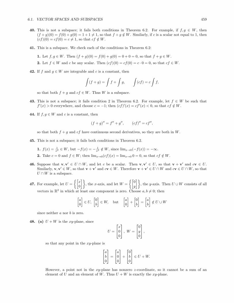
6.1. VECTOR SPACES AND SUBSPACES 459
40. This is not a subspace; it fails both conditions in Theorem 6.2. For example, if f, g ∈ W , then(f + g)(0) = f(0) + g(0) = 1 + 1 6= 1, so that f + g /∈W . Similarly, if c is a scalar not equal to 1, then(cf)(0) = cf(0) = c 6= 1, so that cf /∈W .
41. This is a subspace. We check each of the conditions in Theorem 6.2:
1. Let f, g ∈W . Then (f + g)(0) = f(0) + g(0) = 0 + 0 = 0, so that f + g ∈W .
2. Let f ∈W and c be any scalar. Then (cf)(0) = cf(0) = c · 0 = 0, so that cf ∈W .
42. If f and g ∈W are integrable and c is a constant, then∫(f + g) =
∫f +
∫g,
∫(cf) = c
∫f,
so that both f + g and cf ∈W . Thus W is a subspace.
43. This is not a subspace; it fails condition 2 in Theorem 6.2. For example, let f ∈ W be such thatf ′(x) > 0 everywhere, and choose c = −1; then (cf)′(x) = cf ′(x) < 0, so that cf /∈W .
44. If f, g ∈W and c is a constant, then
(f + g)′′ = f ′′ + g′′, (cf)′′ = cf ′′,
so that both f + g and cf have continuous second derivatives, so they are both in W .
45. This is not a subspace; it fails both conditions in Theorem 6.2.
1. f(x) = 1x2 ∈W , but −f(x) = − 1
x2 /∈W , since limx→0(−f(x)) = −∞.
2. Take c = 0 and f ∈W ; then limx→0(cf)(x) = limx→0 0 = 0, so that cf /∈W .
46. Suppose that v,v′ ∈ U ∩ W , and let c be a scalar. Then v,v′ ∈ U , so that v + v′ and cv ∈ U .Similarly, v,v′ ∈W , so that v + v′ and cv ∈W . Therefore v + v′ ∈ U ∩W and cv ∈ U ∩W , so thatU ∩W is a subspace.
47. For example, let U =
{[x0
]}, the x-axis, and let W =
{[0y
]}, the y-axis. Then U ∪W consists of all
vectors in R2 in which at least one component is zero. Choose a, b 6= 0; then[a0
]∈ U,
[0b
]∈W, but
[a0
]+
[0b
]=
[ab
]/∈ U ∪W
since neither a nor b is zero.
48. (a) U +W is the xy-plane, since
U =
x00
, W =
0y0
,so that any point in the xy-plane isab
0
=
a00
+
0b0
∈ U +W.
However, a point not in the xy-plane has nonzero z-coordinate, so it cannot be a sum of anelement of U and an element of W . Thus U +W is exactly the xy-plane.

460 CHAPTER 6. VECTOR SPACES
(b) Suppose x,x′ ∈ U +W ; say x = u + w and x′ = u′ + w′, where u,u′ ∈ U and w,w′ ∈W . Then
x + x′ = u + w + u′ + w′ = (u + u′) + (w + w′) ∈ U +W
since both U and W are subspaces. If c is a scalar, then
cx = c(u + w) = cu + cw ∈ U +W,
again since both U and W are subspaces.
49. We verify all ten axioms of a vector space. Note that both U and V are vector spaces, so they satisfyall the vector space axioms. These facts will be used without comment below. Let (u1,v1), (u2,v2),and (u3,v3) be elements of U × V , and let c and d be scalars. Then
1. (u1,v1) + (u2,v2) = (u1 + u2,v1 + v2) ∈ U × V .
2. (u1,v1) + (u2,v2) = (u1 + u2,v1 + v2) = (u2 + u1,v2 + v1) = (u2,v2) + (u1,v1).
3.
((u1,v1) + (u2,v2)) + (u3,v3) = (u1 + u2,v1 + v2) + (u3,v3)
= ((u1 + u2) + u3, (v1 + v2) + v3)
= (u1 + (u2 + u3),v1 + (v2 + v3))
= (u1,v1) + (u2 + u3,v2 + v3)
= (u1,v1) + ((u2,v2) + (u3,v3)).
4. (0,0) ∈ U × V , and (u1,v1) + (0,0) = (u1 + 0,v1 + 0) = (u1,v1).
5. (u1,v1) + (−u1,−v1) = (u1 − u1,v1 − v1) = (0,0).
6. c(u1,v1) = (cu1, cv1) ∈ U × V .
7.
c ((u1,v1) + (u2,v2)) = c(u1 + u2,v1 + v2)
= (c(u1 + u2), c(v1 + v2))
= (cu1 + cu2, cv1 + cv2)
= (cu1, cv1) + (cu2, cv2)
= c(u1,v1) + c(u2,v2).
8.
(c+ d)(u1,v1) = ((c+ d)u1, (c+ d)v1)
= (cu1 + du1, cv1 + dv1)
= (cu1, cv1) + (du1, dv1)
= c(u1,v1) + d(u1,v1).
9. c (d(u1,v1)) = c(du1, dv1) = (c(du1), c(du2)) = ((cd)u1, (cd)v1) = (cd)(u1,v1).
10. 1(u1,v1) = (1u1, 1v1) = (u1,v1).
50. Suppose that (w,w), (w′,w′) ∈ ∆. Then
(w,w) + (w′,w′) = (w + w′,w + w′),
which is in ∆ since its two components are the same. Let c be a scalar. Then
c(w,w) = (cw, cw),
which is also in ∆ since its components are the same. Therefore ∆ satisfies both conditions of Theorem6.2, so is a subspace.

6.1. VECTOR SPACES AND SUBSPACES 461
51. If aA+ bB = C, then
a
[1 1−1 1
]+ b
[1 −11 0
]=
[a+ b a− bb− a a
]=
[1 23 4
].
Then a− b = 2 and b− a = 3, which is impossible. Therefore C is not in the span of A and B.
52. If aA+ bB = C, then
a
[1 1−1 1
]+ b
[1 −11 0
]=
[a+ b a− bb− a a
]=
[3 −55 −1
].
Then a = −1 from the lower right. The upper left then gives −1+b = 3, so that b = 4. Then a−b = −5and b− a = 5, so that −A+ 4B = C.
53. Suppose that
a(1− 2x) + b(x− x2) + c(−2 + 3x+ x2) = (a− 2c) + (−2a+ b+ 3c)x+ (−b+ c)x2 = 3− 5x− x2.
Then
a − 2c = 3
−2a+ b+ 3c = −5
− b+ c = −1.
The third equation gives b = c + 1; substituting this in the second equation gives −2a + 4c = −6,which is −2 times the first equation. So there is a family of solutions, which can be parametrized asa = 2t+ 3, b = t+ 1, c = t. For example, with t = 0 we get
s(x) = 3p(x) + q(x),
and s(x) ∈ span(p(x), q(x), r(x)).
54. Suppose that
a(1− 2x) + b(x− x2) + c(−2 + 3x+ x2) = (a− 2c) + (−2a+ b+ 3c)x+ (−b+ c)x2 = 1 + x+ x2.
Then
a − 2c = 1
−2a+ b+ 3c = 1
− b+ c = 1.
The third equation gives b = c − 1; substituting into the second equation gives −2a + 4c − 1 = 1,or a − 2c = −1. This conflicts with the first equation, so the system has no solution. Thus s(x) /∈span(p(x), q(x), r(x)).
55. Since sin2 x+ cos2 x = 1, we have 1 = f(x) + g(x) ∈ span(sin2 x, cos2 x).
56. Since cos 2x = cos2 x− sin2 x = g(x)− f(x), we have cos 2x = −f(x) + g(x) ∈ span(sin2 x, cos2 x).
57. Suppose that sin 2x = af(x) + bg(x) = a sin2 x+ b cos2 x for all x. Then
Let x = 0; then 0 = a sin2 0 + b cos2 0 = b, so that b = 0.
Let x =π
2; then sin
(2 · π
2
)= sinπ = 0 = a sin2 π
2+ b cos2 π
2= a, so that a = 0.
Thus the only solution is a = b = 0, but this is not a valid solution since sin 2x 6= 0. So sin 2x /∈span(sin2 x, cos2 x).

462 CHAPTER 6. VECTOR SPACES
58. Suppose that sinx = af(x) + bg(x) = a sin2 x+ b cos2 x for all x. Then
Let x = 0; then 0 = a sin2 0 + b cos2 0 = b, so that b = 0.
Let x =π
2; then sin
π
2= 1 = a sin2 π
2+ b cos2 π
2= a, so that a = 1.
Thus the only possibility is sinx = sin2 x. But this is not a valid equation; for example, if x = 3π2 ,
then the left-hand side is −1 while the right-hand side is 1. So sinx /∈ span(sin2 x, cos2 x).
59. Let
V1 =
[1 10 1
], V2 =
[0 11 0
], V3 =
[1 01 1
], V4 =
[0 −11 0
].
Now, V4 = V3 − V1, so that span(V1, V2, V3, V4) = span(V1, V2, V3). If span(V1, V2, V3) = M22, thenevery matrix is in the span, so in particular E11 is. But
aV1 + bV2 + cV3 = E11 ⇒[a+ c a+ bb+ c a+ c
]=
[1 00 0
].
Now the diagonal entries give a+ c = 0 and a+ c = 1, which has no solution. So E11 is not in the spanand thus span(V1, V2, V3) 6= M22.
60. Let
V1 =
[1 01 0
], V2 =
[1 11 0
], V3 =
[1 11 1
], V4 =
[0 −11 0
].
Solving the four independent systems
E11 = aV1 + bV2 + cV3 + dV4 E12 = aV1 + bV2 + cV3 + dV4
E21 = aV1 + bV2 + cV3 + dV4 E22 = aV1 + bV2 + cV3 + dV4
gives
E11 = 2V1 − V2 − V4 E12 = −V1 + V2
E21 = −V1 + V2 + V4 E22 = −V2 + V3.
Therefore span(V1, V2, V3, V4) ⊇ span(E11, E12, E21, E22) = M22.
61. Let p(x) = 1 + x, q(x) = x+ x2, and r(x) = 1 + x2. Then
1 = ap(x) + bq(x) + cs(x) ⇒a + c = 1a + b = 0
b + c = 0⇒ a =
1
2, b = −1
2, c =
1
2
x = ap(x) + bq(x) + cs(x) ⇒a + c = 0a + b = 1
b + c = 0⇒ a =
1
2, b =
1
2, c = −1
2
x2 = ap(x) + bq(x) + cs(x) ⇒a + c = 0a + b = 0
b + c = 1⇒ a = −1
2, b =
1
2, c =
1
2.
Thus span(p(x), q(x), r(x)) ⊇ span(1, x, x2) = P2.
62. Let p(x) = 1 + x+ 2x2, q(x) = 2 + x+ 2x2, and r(x) = −1 + x+ 2x2. Then
x = ap(x) + bq(x) + cs(x) ⇒a + 2b − c = 0a + b + c = 1
2a + 2b + 2c = 0 .
But the second pair of equations are inconsistent, so that x /∈ span(p(x), q(x), r(x)). Thereforespan(p(x), q(x), r(x)) 6= P2.
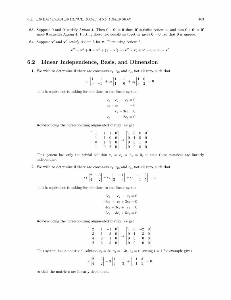
6.2. LINEAR INDEPENDENCE, BASIS, AND DIMENSION 463
63. Suppose 0 and 0′ satisfy Axiom 4. Then 0 + 0′ = 0 since 0′ satisfies Axiom 4, and also 0 + 0′ = 0′
since 0 satisfies Axiom 4. Putting these two equalities together gives 0 = 0′, so that 0 is unique.
64. Suppose v′ and v′′ satisfy Axiom 5 for v. Then using Axiom 5,
v′′ = v′′ + 0 = v′′ + (v + v′) = (v′′ + v) + v′ = 0 + v′ = v′.
6.2 Linear Independence, Basis, and Dimension
1. We wish to determine if there are constants c1, c2, and c3, not all zero, such that
c1
[1 10 −1
]+ c2
[1 −11 0
]+ c3
[1 03 2
]= 0.
This is equivalent to asking for solutions to the linear system
c1 + c2 + c3 = 0
c1 − c2 = 0
c2 + 3c3 = 0
−c1 + 2c3 = 0.
Row-reducing the corresponding augmented matrix, we get1 1 1 01 −1 0 00 1 3 0−1 0 2 0
→
1 0 0 00 1 0 00 0 1 00 0 0 0
.This system has only the trivial solution c1 = c2 = c3 = 0, so that these matrices are linearlyindependent.
2. We wish to determine if there are constants c1, c2, and c3, not all zero, such that
c1
[2 −34 2
]+ c2
[1 −13 3
]+ c3
[−1 3
1 5
]= 0.
This is equivalent to asking for solutions to the linear system
2c1 + c2 − c3 = 0
−3c1 − c2 + 3c3 = 0
4c1 + 3c2 + c3 = 0
2c1 + 3c2 + 5c3 = 0.
Row-reducing the corresponding augmented matrix, we get2 1 −1 0−3 −1 3 0
4 3 1 02 3 5 0
→
1 0 −2 00 1 3 00 0 0 00 0 0 0
.This system has a nontrivial solution c1 = 2t, c2 = −3t, c3 = t; setting t = 1 for example gives
2
[2 −34 2
]− 3
[1 −13 3
]+
[−1 3
1 5
]= 0.
so that the matrices are linearly dependent.

464 CHAPTER 6. VECTOR SPACES
3. We wish to determine if there are constants c1, c2, c3, and c4, not all zero, such that
c1
[−1 1−2 2
]+ c2
[3 01 1
]+ c3
[0 2−3 1
]+ c4
[−1 0−1 7
]= 0.
This is equivalent to asking for solutions to the linear system
−c1 + 3c2 − c4 = 0
c1 + 2c3 = 0
−2c1 + c2 − 3c3 − c4 = 0
2c1 + c2 + c3 + 7c4 = 0.
Row-reducing the corresponding augmented matrix, we get−1 3 0 −1 0
1 0 2 0 0−2 1 −3 −1 0
2 1 1 7 0
→
1 0 0 4 00 1 0 1 00 0 1 −2 00 0 0 0 0
.This system has a nontrivial solution c1 = −4t, c2 = −t, c3 = 2t, c4 = t; setting t = 1 for examplegives
−4
[−1 1−2 2
]−[3 01 1
]+ 2
[0 2−3 1
]+
[−1 0−1 7
]= 0.
so that the matrices are linearly dependent.
4. We wish to determine if there are constants c1, c2, c3, and c4, not all zero, such that
c1
[1 10 1
]+ c2
[1 01 1
]+ c3
[0 11 1
]+ c4
[1 11 0
]= 0.
This is equivalent to asking for solutions to the linear system
c1 + c2 + c4 = 0
c1 + c3 + c4 = 0
c2 + c3 + c4 = 0
c1 + c2 + c3 = 0.
Row-reducing the corresponding augmented matrix, we get1 1 0 1 01 0 1 1 00 1 1 1 01 1 1 0 0
→
1 0 0 0 00 1 0 0 00 0 1 0 00 0 0 1 0
.Since the only solution is the trivial solution, it follows that these four matrices are linearly independentover M22.
5. Following, for instance, Example 6.26, we wish to determine if there are constants c1 and c2, not bothzero, such that
c1(x) + c2(1 + x) = 0.
This is equivalent to asking for solutions to the linear system
c2 = 0
c1 + c2 = 0.
By forward substitution, we see that the only solution is the trivial solution, c1 = c2 = 0. It followsthat these polynomials are linearly independent over P2.

6.2. LINEAR INDEPENDENCE, BASIS, AND DIMENSION 465
6. Following, for instance, Example 6.26, we wish to determine if there are constants c1, c2, and c3, notall zero, such that
c1(1 + x) + c2(1 + x2) + c3(1− x+ x2) = (c1 + c2 + c3) + (c1 − c3)x+ (c2 + c3)x2 = 0.
This is equivalent to asking for solutions to the linear system
c1 + c2 + c3 = 0
c1 − c3 = 0
c2 + c3 = 0.
Row-reducing the corresponding augmented matrix, we get1 1 1 01 0 −1 00 1 1 0
→1 0 0 0
0 1 0 00 0 1 0
.Since the only solution is the trivial solution, it follows that these three polynomials are linearlyindependent over P2.
7. Following, for instance, Example 6.26, we wish to determine if there are constants c1, c2, and c3, notall zero, such that
c1(x) + c2(2x− x2) + c3(3x+ 2x2) = (c1 + 2c2 + 3c3)x+ (−c2 + 2c3)x2 = 0.
This is a homogeneous system of two equations in three unknowns, so we know it has a nontrivialsolution and these polynomials are linearly dependent. To find an expression showing the lineardependence, we must find solutions to the linear system
c1 + 2c2 + 3c3 = 0
− c2 + 2c3 = 0.
Row-reducing the corresponding augmented matrix, we get[1 2 3 00 −1 2 0
]→[1 0 7 00 1 −2 0
].
The general solution is c1 = −7t, c2 = 2t, c3 = t. Setting t = 1, for example, we get
−7(x) + 2(2x− x2) + (3x+ 2x2) = 0.
8. Following, for instance, Example 6.26, we wish to determine if there are constants c1, c2, c3, and c4,not all zero, such that
c1(2x)+c2(x−x2)+c3(1+x3)+c4(2−x2 +x3) = (c3 +2c4)+(2c1 +c2)x+(−c2−c4)x2 +(c3 +c4)x3 = 0.
This is equivalent to asking for solutions to the linear system
c3 + 2c4 = 0
2c1 + c2 = 0
− c2 − c4 = 0
c3 + c4 = 0.
Row-reducing the corresponding augmented matrix, we get0 0 1 2 02 1 0 0 00 −1 0 −1 00 0 1 1 0
→
1 0 0 0 00 1 0 0 00 0 1 0 00 0 0 1 0
.Since the only solution is the trivial solution, it follows that these four polynomials are linearly inde-pendent over P3.

466 CHAPTER 6. VECTOR SPACES
9. Following, for instance, Example 6.26, we wish to determine if there are constants c1, c2, c3, and c4,not all zero, such that
c1(1− 2x) + c2(3x+ x2 − x3) + c3(1 + x2 + 2x3) + c4(3 + 2x+ 3x3)
= (c1 + c3 + 3c4) + (−2c1 + 3c2 + 2c4)x+ (c2 + c3)x2 + (−c2 + 2c3 + 3c4)x3 = 0.
This is equivalent to asking for solutions to the linear system
c1 + c3 + 3c4 = 0
−2c1 + 3c2 + 2c4 = 0
c2 + c3 = 0
− c2 + 2c3 + 3c4 = 0.
Row-reducing the corresponding augmented matrix, we get1 0 1 3 0−2 3 0 2 0
0 1 1 0 00 −1 2 3 0
→
1 0 0 0 00 1 0 0 00 0 1 0 00 0 0 1 0
.Since the only solution is the trivial solution, it follows that these four polynomials are linearly inde-pendent over P3.
10. We wish to find solutions to a+ b sinx+ c cosx = 0 that hold for all x. Setting x = 0 gives a+ c = 0,so that a = −c; setting x = π gives a− c = 0, so that a = c. This forces a = c = 0; then setting x = π
2gives b = 0. So the only solution is the trivial solution, and these functions are linearly independent inF .
11. Since sin2 x+ cos2 x = 1, the functions are linearly dependent.
12. Suppose that aex + be−x = 0 for all x. Setting x = 0 gives ae0 + be0 = a+ b = 0, while setting x = ln 2gives 2a+ 1
2b = 0. Since the coefficient matrix,[1 1
2 12
],
has nonzero determinant, the only solution to the system is the trivial solution, so that these functionsare linearly independent in F .
13. Using properties of the logarithm, we have ln(2x) = ln 2 + lnx and ln(x2) = 2 lnx, so we want to seeif {1, ln 2 + lnx, 2 lnx} are linearly independent over F . But clearly they are not, since by inspection
(−2 ln 2) · 1 + 2 · (ln 2 + lnx)− 2 lnx = 0.
So these functions are linearly dependent in F .
14. We wish to find solutions to a sinx+ b sin 2x+ c sin 3x = 0 that hold for all x. Setting
x =π
2⇒ a− c = 0
x =π
6⇒ 1
2a+
√3
2b = 0
x =π
3⇒
√3
2a−√
3
2b = 0.
Adding the second and third equations gives(
12 +
√3
2
)a = 0, so that a = 0; then the first and third
equations force b = c = 0. So the only solution is the trivial solution, and thus these functions arelinearly independent in F .

6.2. LINEAR INDEPENDENCE, BASIS, AND DIMENSION 467
15. We want to prove that if the Wronskian is not identically zero, then f and g are linearly independent.We do this by proving the contrapositive: assume f and g are linearly dependent. If either f or g iszero, then clearly the Wronskian is zero as well. So assume that neither f nor g is zero; since they arelinearly dependent, each is a nonzero multiple of the other. Say f(x) = ag(x), so that f ′(x) = ag′(x).Now, the Wronskian is∣∣∣∣f(x) g(x)f ′(x) g′(x)
∣∣∣∣ = f(x)g′(x)− g(x)f ′(x) = ag(x)g′(x)− g(x)(ag′(x)) = ag(x)g′(x)− ag(x)g′(x) = 0.
Thus the Wronskian is identically zero, proving the result.
16. Exercise 10: W (x) =
∣∣∣∣∣∣1 sinx cosx0 cosx − sinx0 − sinx − cosx
∣∣∣∣∣∣ =
∣∣∣∣ cosx − sinx− sinx − cosx
∣∣∣∣ = − cos2 x−sin2 x = −1 6= 0. Since
the Wronskian is not zero, the functions are linearly independent.
Exercise 11:
W (x) =
∣∣∣∣∣∣1 sin2 x cos2 x0 2 sinx cosx −2 sinx cosx0 2(cos2 x− sin2 x) 2(sin2 x− cos2 x)
∣∣∣∣∣∣=
∣∣∣∣∣∣1 sin2 x cos2 x0 sin 2x − sin 2x0 2 cos 2x −2 cos 2x
∣∣∣∣∣∣=
∣∣∣∣ sin 2x − sin 2x2 cos 2x −2 cos 2x
∣∣∣∣= 0.
Since the Wronskian is zero, the functions are linearly dependent.
Exercise 12: W (x) =
∣∣∣∣ex e−x
ex −e−x∣∣∣∣ = −1 − 1 = −2 6= 0. Since the Wronskian is not zero, the
functions are linearly independent.
Exercise 13:
W (x) =
∣∣∣∣∣∣∣1 ln(2x) ln(x2)
0 1x
2x
0 − 1x2 − 2
x2
∣∣∣∣∣∣∣ =
∣∣∣∣∣ 1x
2x
− 1x2 − 2
x2
∣∣∣∣∣ = 0.
Since the Wronskian is zero, the functions are linearly dependent.
Exercise 14: W (x) =
∣∣∣∣∣∣sinx sin 2x sin 3xcosx 2 cos 2x 3 cos 3x− sinx −4 sin 2x −9 sin 3x
∣∣∣∣∣∣. Rather than computing the determinant and
showing it is not identically zero, it suffices to find some value of x such that W (x) 6= 0. Letx = π
3 ; then
W(π
3
)=
∣∣∣∣∣∣∣∣sin π
3 sin 2π3 sinπ
cos π3 2 cos 2π3 3 cosπ
− sin π3 −4 sin 2π
3 −9 sinπ
∣∣∣∣∣∣∣∣=
∣∣∣∣∣∣∣∣√
32
√3
2 012 −1 −3
−√
32 −2
√3 0
∣∣∣∣∣∣∣∣= 3
∣∣∣∣∣√
32
√3
2
−√
32 −2
√3
∣∣∣∣∣= 3
(−3 +
3
4
)= −27
46= 0.

468 CHAPTER 6. VECTOR SPACES
So the Wronskian is not identically zero and therefore the functions are linearly independent.
17. (a) Yes, it is. Suppose
a(u + v) + b(v + w) + c(u + w) = (a+ c)u + (a+ b)v + (b+ c)w = 0.
Since {u,v,w} are linearly independent, it follows that a + c = 0, a + b = 0, and b + c = 0.Subtracting the latter two from each other gives a− c = 0; combining this with the first equationshows that a = c = 0, and then b = 0. So the only solution to the system is the trivial one, sothese three vectors are linearly independent.
(b) No, they are not, since
(u− v) + (v −w)− (u−w) = 0.
18. Since dimM22 = 4 but B has only three elements, it cannot be a basis.
19. If
a
[1 00 1
]+ b
[0 −11 0
]+ c
[1 11 1
]+ d
[1 11 −1
]=
[0 00 0
],
then
a + c+ d = 0
− b+ c+ d = 0
b+ c+ d = 0
a + c− d = 0.
Subtracting the second and third equations shows that b = 0; subtracting the first and fourth showsthat d = 0. Then from the second equation, c = 0 as well, which forces a = 0. So the only solutionis the trivial solution, and these matrices are linearly independent. Since there are four of them, anddimM22 = 4, it follows that they form a basis for M22.
20. Since dimM22 = 4, if these vectors are linearly independent then they span and thus form a basis. Tosee if they are linearly independent, we want to solve
c1
[1 00 1
]+ c2
[0 11 0
]+ c3
[1 10 1
]+ c4
[1 01 1
]= 0.
Solving this linear system gives c1 = −2c4, c2 = −c4, and c3 = c4. For example, letting c4 = 1 gives
−2
[1 00 1
]−[0 11 0
]+
[1 10 1
]+
[1 01 1
]= 0.
Thus the matrices are linearly dependent so do not form a basis (see Theorem 6.10).
21. Since dimM22 = 4 but B has five elements, it cannot be a basis.
22. Since dim P2 = 3, if these vectors are linearly independent then they span and thus form a basis. Tosee if they are linearly independent, we want to solve
c1x+ c2(1 + x) + c3(x− x2) = c2 + (c1 + c2 + c3)x− c3x2 = 0.
Rather than setting up the augmented matrix and row-reducing it, simply note that the first and thirdterms force c2 = c3 = 0; then the second term forces c1 = 0. So the only solution is the trivial solution,and these three polynomials are linearly independent, so they form a basis for P2.

6.2. LINEAR INDEPENDENCE, BASIS, AND DIMENSION 469
23. Since dim P2 = 3, if these vectors are linearly independent then they span and thus form a basis. Tosee if they are linearly independent, we want to solve
c1(1− x) + c2(1− x2) + c3(x− x2) = (c1 + c2) + (−c1 + c3)x+ (−c2 − c3)x2 = 0.
To solve the resulting linear system, we row-reduce its augmented matrix: 1 1 0 0−1 0 1 0
0 −1 −1 0
→1 0 −1 0
0 1 1 00 0 0 0
.This has general solution c1 = t, c2 = −t, c3 = t, so setting t = 1 we get
(1− x)− (1− x2) + (x− x2) = 0.
Therefore the vectors are not linearly independent, so they cannot form a basis for P2, which hasdimension 3.
24. Since dim P2 = 3 but there are only two vectors in B, they cannot form a basis.
25. Since dim P2 = 3 but there are four vectors in B, they must be linearly dependent, so cannot form abasis.
26. We want to find constants c1, c2, c3, and c4 such that
c1E22 + c2E21 + c3E12 + c4E11 = A =
[1 23 4
].
Setting up the equivalent linear system gives
c1 = 4
c2 = 3
c3 = 2
c4 = 1.
This system obviously has the solution c1 = 4, c2 = 3, c3 = 2, c4 = 1, so the coordinate vector is
[A]B =
4321
.27. We want to find constants c1, c2, c3, and c4 such that
c1
[1 00 0
]+ c2
[1 10 0
]+ c3
[1 11 0
]+ c4
[1 11 1
]=
[1 23 4
].
Setting up the equivalent linear system gives
c1 + c2 + c3 + c4 = 1
c2 + c3 + c4 = 2
c3 + c4 = 3
c4 = 4.
By backwards substitution, the solution is c4 = 4, c3 = −1, c2 = −1, c1 = −1, so the coordinate vectoris
[A]B =
−1−1−1
4
.

470 CHAPTER 6. VECTOR SPACES
28. We want to find constants c1, c2, and c3 such that
p(x) = 1 + 2x+ 3x2 = c1(1 + x) + c2(1− x) + c3(x2) = (c1 + c2) + (c1 − c2)x+ c3x2.
The corresponding linear system is
c1 + c2 = 1
c1 − c2 = 2
c3 = 3.
Row-reducing the corresponding augmented matrix gives1 1 0 1
1 −1 0 2
0 0 1 3
→
1 0 0 32
0 1 0 − 12
0 0 1 3
,so that c1 = 3
2 , c2 = − 12 , and c3 = 3. Thus the coordinate vector is
[p]B =
32
− 12
3
.29. We want to find constants c1, c2, and c3 such that
p(x) = 2− x+ 3x2 = c1(1) + c2(1 + x) + c3(−1 + x2) = (c1 + c2 − c3) + c2x+ c3x2.
Equating coefficients shows that c3 = 3 and c2 = −1; substituting into the equation c1 + c2 − c3 = 2gives c1 = 6, so that the coordinate vector is
[p]B =
6−1
3
.30. To show B is a basis, we must show that it spans V and that the elements of B are linearly independent.B spans V , since if v ∈ V , then it can be written as a linear combination of vectors in B by hypothesis.To show they are linearly independent, note that 0 =
∑0ui; since the representation of 0 is unique
by assumption, it follows that the only solution to 0 =∑ciui is the trivial solution, so that B = {ui}
is a linearly independent set. Thus B is a basis for V .
31. [c1u1 + · · ·+ ckuk]B = [c1u1]B + · · ·+ [ckuk]B = c1[u1]B + · · ·+ ck[uk]B.
32. Suppose c1u1 + · · ·+ cnun = 0. Then clearly
0 = [c1u1 + · · ·+ cnun]B.
But by Exercise 31, the latter expression is equal to
c1[u1]B + · · ·+ cn[un]B;
since [ui]B are linearly independent in Rn, we get ci = 0 for all i, so that the only solution to theoriginal equation is the trivial solution. Thus the ui are linearly independent in V .
33. First suppose that span(u1, . . . ,um) = V . Choose
x =
c1c2...cn
∈ Rn.

6.2. LINEAR INDEPENDENCE, BASIS, AND DIMENSION 471
Then∑ciui ∈ V since V = span(ui). Therefore by Exercise 31
x = [c1u1 + · · ·+ cmum]B = c1[u1]B + · · ·+ cm[um]B,
which shows that x ∈ span(S).
For the converse, suppose that span(S) = Rn. Choose v ∈ V ; then [v]B ∈ Rn, and using Exercise 31again,
[v]B =∑
ci[ui]B =[∑
ciui
]B.
But since B is a basis, and the two elements v and∑ciui of V have the same coordinate vector, they
must be the same element. Thus v =∑ciui, so that {ui} spans V .
34. Using the standard basis {x2, x, 1} for P2, if p(x) = ax2 + bx+ c ∈ V , then p(0) = c = 0, so that c = 0and therefore p(x) = ax2 + bx. Since x2 and x are linearly independent and span V , {x, x2} is a basis,so that dimV = 2.
35. Two polynomials in V are p(x) = 1 − x and q(x) = 1 − x2, since p(1) = q(1) = 0. If we show thesepolynomials are linearly independent and span V , we are done. They are linearly independent, since if
a(1− x) + b(1− x2) = (a+ b)− ax− bx2 = 0,
then equating coefficients shows that a = b = 0. To see that they span, suppose r(x) = c+bx+ax2 ∈ V .Then r(1) = a+ b+ c = 0, so that c = −b− a and therefore
r(x) = −(b+ a) + bx+ ax2 = −b(1− x)− a(1− x2),
so that r is a linear combination of p and q. Thus {p(x), q(x)} forms a basis for V , which has dimension2.
36. Suppose p(x) = c+ bx+ ax2; then xp′(x) = bx+ 2ax2. So p(x) = xp′(x) means that c = 0 and a = 2a,so that a = 0. Thus p(x) = bx. Then clearly V = span(x), so that {x} forms a basis, and dimV = 1.
37. Upper triangular matrices in M22 have the form[a b0 d
]= aE11 + bE12 + dE22.
Since E11, E12, and E22 span V , and we know they are linearly independent, it follows that they forma basis for V , which therefore has dimension 3.
38. Skew-symmetric matrices in M22 have the form[0 b−b 0
]= b
[0 1−1 0
]= bA.
Since A spans V , and {A} is a linearly independent set, we see that {A} is a basis for V , which thereforehas dimension 1.
39. Suppose that
A =
[a bc d
].
Then
AB =
[a a+ bc c+ d
], BA =
[a+ c b+ dc d
].
Then AB = BA means that a = a + c, so that c = 0, and also a + b = b + d, so that a = d. So thematrix A has the form
A =
[a b0 a
]= a
[1 00 1
]+ bE12 = aI + bE12.
I and E12 are linearly independent since I = E11 +E22, and {E11, E22, E12} is a linearly independentset. Since they span, we see that {I, E12} forms a basis for V , which therefore has dimension 2.

472 CHAPTER 6. VECTOR SPACES
40. dimMnn = n2. For symmetric matrices, we have aij = aji. Therefore specifying the entries on orabove the diagonal determines the matrix, and these entries may take any value. Since there are
n+ (n− 1) + · · ·+ 2 + 1 =n(n+ 1)
2
entries on or above the diagonal, this is the dimension of the space of symmetric matrices.
41. dimMnn = n2. For skew-symmetric matrices, we have aij = −aji. Therefore all the diagonal entriesare zero; further, specifying the entries above the diagonal determines the matrix, and these entriesmay take any value. Since there are
(n− 1) + · · ·+ 2 + 1 =n(n− 1)
2
entries above the diagonal, this is the dimension of the space of symmetric matrices.
42. Following the hint, Let B = {v1, . . . ,vk} be a basis for U ∩ W . By Theorem 6.10(e), this can beextended to a basis C for U and to a basis D for W . Consider the set C ∪ D. Clearly it spans U +W ,since an element of U+W is u+w for u ∈ U , w ∈W ; since C and D are bases for U and W , the resultfollows. Next we must show that this set is linearly independent. Suppose dimU = m and dimV = n;then
C = {uk+1, . . . ,um} ∪ B, D = {wk+1, . . . ,wn} ∪ B.
Suppose that a linear combination of C ∪ D is the zero vector. This means that
a1v1 + · · ·+ akvk + ck+1uk+1 + · · ·+ cmum + dk+1wk+1 + dnwn = A+ C +D = 0.
This means that C = −A − D. Since A ∈ U ∩W and D ∈ W , we see that −A − D ∈ W so thatC ∈ W . But also C ∈ U , since it is a combination of basis vectors for U . Thus C ∈ U ∩W , which isimpossible unless all of the ci are zero, since the uk+1 are elements of U not in the subspace U ∩W .We are left with A+D = 0; this is a linear combination of basis elements of W , so that all the ai andall the dj must be zero as well. Therefore C ∪ D is linearly independent.
It follows that C ∪ D forms a basis for U +W , so it remains to count the elements in this set. ClearlyC ∩ D = B, for any basis element in common between C and D must be in U ∩W , so it must be in B.Write #X for the number of elements in the set X. Then
dim(U +W ) = #(C ∪ D) = #C + #D −#B = n+m− k = dimU + dimW − dim(U ∩W ).
43. Let dimU = m, with basis B = {u1, . . . ,um}, and dimV = n, with basis C = {v1, . . . ,vn}.
(a) Claim that a basis for U ×V is D = {(ui,0), (0,vj)}. This will also show that dim(U ×V ) = mn,by counting the basis vectors. First we want to show that D spans. Let x = (u,v) ∈ U × V .Then
x = (u,v) =
m∑i=1
ciui,
n∑j=1
djvj
=
m∑i=1
ci(ui,0) +
n∑j=1
dj(0,vj),
proving that D spans U × V . To see that D is linearly independent, suppose that 0 is a linearcombination of the elements of D. This means that
0 = (0,0) =
m∑i=1
ci(ui,0) +
n∑j=1
dj(0,vj) =
m∑i=1
ciui,
n∑j=1
djvj
.
But the ui are linearly independent, so that∑mi=1 ciui = 0 means that all of the ci are zero;
similarly the vj are linearly independent, so that∑nj=1 djvj = 0 means that all of the dj are zero.
Thus D is linearly independent.
So D is a basis for U ×W , and therefore dim(U ×W ) = mn.
6.2. LINEAR INDEPENDENCE, BASIS, AND DIMENSION 473
(b) Let dimW = k, with basis {w1, . . . ,wk}. Claim that D = {(wi,wi)} is a basis for ∆; provingthis claim also shows, by counting the basis vectors, that dim ∆ = dimW . To see that D spans∆, choose (w,w) ∈ ∆; then w =
∑ciwi, so that
(w,w) =(∑
ciwi,∑
ciwi
)=∑
(ciwi, ciwi) =∑
ci(wi,wi).
Thus D spans ∆. To see that D is linearly independent, suppose that∑ci(wi,wi) = 0. Then
0 =∑
ci(wi,wi) =∑
(ciwi, ciwi) =(∑
ciwi,∑
ciwi
).
This means that∑ciwi = 0; since the wi are linearly independent, we see that all the ci are
zero. So D is linearly independent, showing that it is a basis for ∆ and thus that dim ∆ = dimW .
44. Suppose that P is finite dimensional, and that {p1(x), . . . , pn(x)} is a basis. Let m be the largest powerof x that appears in any of the basis elements, and consider q(x) = xm+1. Since any linear combinationof the pi has powers of x at most equal to m, it follows that q /∈ span{pi}, so that P cannot have afinite basis.
45. Start by adding all three standard basis vectors for P2 to the set, yielding {1 + x, 1 + x+ x2, 1, x, x2}.Since (1 + x) + x2 = 1 + x+ x2, we see that {1 + x, 1 + x+ x2, x2} is linearly dependent, so discard x2,leaving {1 + x, 1 + x+ x2, 1, x}. Next, since (1 + x) = 1 + x, the set {1 + x, 1, x} is linearly dependent,so discard x, leaving B = {1 + x, 1 + x+ x2, 1}. This is a set of three vectors, so to prove that it is abasis, it suffices to show that it spans. But by construction, the standard basis vectors not in B arelinear combinations of elements of B. Hence B is a basis for P2.
46. Start by adding the standard basis vectors Eij to the set, giving
B =
{C =
[0 10 1
], D =
[1 10 1
], E11, E12, E21, E22
}.
Since E11 = D − C is the difference of the two given matrices, we discard it from B, leaving us withfive elements. Next, C = E12 + E22, so discard E22, leaving us with B = {C,D,E12, E21}. This hasfour elements, and dimM22 = 4, so to prove that this is a basis, it suffices to prove that it spans. Butby construction, the standard basis vectors not in B are linear combinations of elements of B. So Bspans and therefore forms a basis for M22.
47. Start by adding the standard basis vectors Eij to the set, giving
B =
{I =
[1 00 1
], C =
[0 11 0
], D =
[0 −11 0
], E11, E12, E21, E22
}.
Since E21 = 12 (C + D), we discard it from B. Next, I = E11 + E22, so discard E22 from B. Finally,
E12 = 12 (C − D), so we discard it from B. This leaves us with B = {I, C,D,E11}. This has four
elements, and dimM22 = 4, so to prove that this is a basis, it suffices to prove that it spans. But byconstruction, the standard basis vectors not in B are linear combinations of elements of B. So B spansand therefore forms a basis for M22.
48. Start by adding the standard basis vectors Eij to the set, giving
B =
{I =
[1 00 1
], C =
[0 11 0
], E11, E12, E21, E22
}.
Since I + C = E11 + E12 + E21 + E22, these are a linearly dependent set; discard E22 from B. Next,C = E12 + E21, so discard E21 from B. This leaves us with B = {I, C,E11, E12}. This has fourelements, and dimM22 = 4, so to prove that this is a basis, it suffices to prove that it spans. But byconstruction, the standard basis vectors not in B are linear combinations of elements of B. So B spansand therefore forms a basis for M22.
474 CHAPTER 6. VECTOR SPACES
49. The standard basis for P1 is {1, x}. If we show that each of these vectors is in the span of the givenvectors, then those vectors span P1. But 1 ∈ span(1, 1+x, 2x), and x = (1+x)−1 ∈ span(1, 1+x, 2x).Thus
span(1, 1 + x, 2x) ⊇ span(1, x) = P1,
so that a basis for the span is {1, x}.
50. Since (1− 2x) + (2x− x2) = 1− x2, these three elements are linearly independent, so we can discard1 − x2 from the set without changing the span, leaving {1 − 2x, 2x − x2, 1 + x2}. Claim these arelinearly independent. Suppose that
a(1− 2x) + b(2x− x2) + c(1 + x2) = (a+ c) + (−2a+ 2b)x+ (−b+ c)x2 = 0.
Then a = −c and a = b from the constant term and the coefficient of x, so that b = −c. But thenb = −c together with −b+ c = 0 shows that b = c = 0, so that a = 0. Hence these three polynomialsare linearly independent, so they form a basis for the span of the original set.
51. Since (1− x) + (x− x2) = 1− x2 and (1− x)− (x− x2) = 1− 2x+ x2, we can remove both 1− x2 and1− 2x+ x2 from the set without changing the span. This leaves us with {1− x, x− x2}. Claim theseare linearly independent. Suppose that
a(1− x) + b(x− x2) = a+ (−a+ b)x− bx2 = 0.
Then clearly a = b = 0. Hence these two polynomials are linearly independent, so they form a basisfor the span of the original set.
52. Let
V1 =
[1 00 1
], V2 =
[0 11 0
], V3 =
[−1 1
1 −1
], V4 =
[1 −1−1 1
].
Then V3 + V4 = 0, so we can discard V4 from the set without changing the span. Next, V3 = V2 − V1,so we can discard V3 from the set without changing the span. So we are left with {V1, V2}; these arelinearly independent since they are not scalar multiples of one another. So this set forms a basis forthe span of the given set.
53. Since cos 2x = cos2 x− sin2 x, we can discard cos 2x from the set without changing the span, leaving uswith {sin2 x, cos2 x}. Claim that this set is linearly independent. For suppose that a sin2 x+b cos2 x = 0holds for all x. Setting x = 0 gives b = 0, while setting x = π
2 gives a = 0. Thus a = b = 0 and these
functions are linearly independent. So {sin2 x, cos2 x} forms a basis for the span of the original set.
54. Suppose that av + c1v1 + · · · + cnvn = 0, so that c1v1 + · · · + cnvn = −av. If a 6= 0, then dividingthrough by −a shows that v ∈ span(S), a contradiction. Therefore we must have a = 0, and we areleft with
c1v1 + · · ·+ cnvn = 0,
which implies (since the vi are linearly independent) that all of the ci are zero. Therefore all coefficientsmust be zero, so that S′ is linearly independent.
55. If vn ∈ span(v1, . . . ,vn−1), then there are constants such that
vn = c1v1 + · · ·+ cn−1vn−1.
Now choose x ∈ V = span(S). Then
x = a1v1 + · · ·+ an−1vn−1 + anvn
= a1v1 + · · ·+ an−1vn−1 + an(c1v1 + · · ·+ cn−1vn−1)
= (a1 + anc1)v1 + · · ·+ (an−1 + ancn−1)vn−1,
showing that x ∈ span(S′). Then V ⊆ span(S′) ⊆ span(S) = V , so that span(S′) = V .

6.2. LINEAR INDEPENDENCE, BASIS, AND DIMENSION 475
56. Use induction on n. If S = {v1}, then S is linearly independent so is a basis. Next, suppose thestatement is true for all sets that span V and have no more than n−1 elements. Let S = {v1, . . . ,vn}.If S is linearly independent, then it is a basis and we are done. Otherwise it is a linearly dependentset, so we can write some element of S (say, vn after a possible reordering) as a linear combination ofthe other, so that vn ∈ span{v1, · · · ,vn−1}. Then by Exercise 55, we can remove vn from S, givingS ′ = {v1, . . . ,vn−1} that also spans V . By the inductive assumption, S ′ can be made into a basis forV by removing some (possibly no) elements, so S can.
57. Suppose x ∈ V . Since S = {v1, . . . ,vn} is a basis, there are scalars a1, . . . , an such that
x = a1v1 + a2v2 + · · ·+ anvn.
Since the ci are nonzero, we also have
x =a1
c1(c1v1) +
a2
c2v2 + · · ·+ an
cn(cnvn),
so that T = {c1v1, . . . , cnvn} spans V . To show T is linearly independent, the argument is much thesame. Suppose that
b1(c1v1) + b2(c2v2) + · · ·+ bn(cnvn) = (b1c1)v1 + (b2c2)v2 + · · ·+ (bncn)vn = v0.
Since S is linearly independent, it follows that bici = 0 for all i. Since all of the ci are nonzero, all ofthe bi must be zero, so that T is linearly independent. Therefore T is also a basis for V .
58. LetS = {v1,v2, . . . ,vn}, T = {v1,v1 + v2,v1 + v2 + v3, . . . ,v1 + v2 + · · ·+ vn}.
By Exercise 21 in Section 2.3, to show that span(T ) = span(S) = V it suffices to show that everyelement of S is in span(T ) and vice versa. But
vi = (v1 + v2 + · · ·+ vi−1 + vi)− (v1 + v2 + · · ·+ vi−1) ∈ span(T ) and
v1 + · · ·+ vi = (v1) + (v2) + · · ·+ (vi) ∈ span(S).
Thus the two spans are equal. Since S is a basis, and T has the same number of elements as S, it mustalso be a basis, by Theorem 6.10(d).
59. (a)
p0(x) =(x− a1)(x− a2)
(a0 − a1)(a0 − a2)=
(x− 2)(x− 3)
(1− 2)(1− 3)=x2 − 5x+ 6
2=
1
2x2 − 5
2x+ 3
p1(x) =(x− a0)(x− a2)
(a1 − a0)(a1 − a2)=
(x− 1)(x− 3)
(2− 1)(2− 3)=x2 − 4x+ 3
−1= −x2 + 4x− 3
p2(x) =(x− a0)(x− a1)
(a2 − a0)(a2 − a1)=
(x− 1)(x− 2)
(3− 1)(3− 2)=x2 − 3x+ 2
2=
1
2x2 − 3
2x+ 1.
(b) If i = j, then substituting aj for x in the definition of pi gives a numerator equal to the denomi-nator, so that pi(aj) = 1 for i = j. If i 6= j, however, then substituting aj for x in the definitionof pi gives zero, since the term x− aj in the numerator of pi becomes zero. Thus
pi(aj) =
{0 if i 6= j
1 if i = j.
60. (a) Note first that the degree of each pi is n, since there are n factors in the numerator, so thatpi ∈Pn for all i. Suppose that there are constants ci such that
c0p0(x) + c1p1(x) + · · ·+ cnpn(x) = 0.
Then this equation must hold for all x. Substitute ai for x. Then by Exercise 59(b), all pj(ai)for j 6= i vanish, leaving only cipi(ai) = ci. Therefore ci = 0. Since this holds for every i, we seethat all of the ci are zero, so that the pi are linearly independent.
476 CHAPTER 6. VECTOR SPACES
(b) Since dim Pn = n + 1 and there are n + 1 polynomials p0, p1, . . . , pn that span, they must forma basis, by Theorem 6.10(d).
61. (a) This is similar to part (a) of Exercise 60. Suppose that q(x) ∈P, and that
q(x) = c0p0(x) + c1p1(x) + · · ·+ cnpn(x).
Then substituting ai for x gives q(ai) = cipi(ai) = ci, since pj(ai) = 0 for j 6= i by Exercise59(b). Since the pi form a basis for P, any element of P has a unique representation as a linearcombination of the pi, so that unique representation must be the one we just found:
q(x) = q(a0)p0(x) + q(a1)p1(x) + · · ·+ q(an)pn(x).
(b) q(x) passes through the given n+ 1 points if and only if q(ai) = c1. But this is exactly what weproved in part (a). Since the representation is unique in part (a), this is the only such degree npolynomial.
(c) (i) Here a0 = 1, a1 = 2, a2 = 3, so we use the Lagrange polynomials determined in Exercise59(a) and therefore
q(x) = c0p0(x) + c1p1(x) + c2p2(x)
= 6
(1
2x2 − 5
2x+ 3
)−(−x2 + 4x− 3
)− 2
(1
2x2 − 3
2x+ 1
)= 3x2 − 16x+ 19.
(ii) Here a0 = −1, a1 = 0, a2 = 3. We first compute the Lagrange polynomials:
p0(x) =(x− a1)(x− a2)
(a0 − a1)(a0 − a2)=
(x− 0)(x− 3)
(−1− 0)(−1− 3)=x2 − 3x
4=
1
4x2 − 3
4x
p1(x) =(x− a0)(x− a2)
(a1 − a0)(a1 − a2)=
(x− (−1))(x− 3)
(0− (−1))(0− 3)=x2 − 2x− 3
−3= −1
3x2 +
2
3x+ 1
p2(x) =(x− a0)(x− a1)
(a2 − a0)(a2 − a1)=
(x− (−1))(x− 0)
(3− (−1))(3− 0)=x2 + x
12=
1
12x2 +
1
12x.
Using these polynomials, we get
q(x) = c0p0(x) + c1p1(x) + c2p2(x)
= 10
(1
4x2 − 3
4x
)+ 5
(−1
3x2 +
2
3x+ 1
)+ 2
(1
12x2 +
1
12x
)=
(5
2− 5
3+
1
6
)x2 +
(−15
2+
10
3+
1
6
)x+ 5
= x2 − 4x+ 5.
62. Suppose that (a0, 0), (a1, 0), . . . , (an, 0) be the n + 1 distinct zeros. Then by Exercise 61(a), the onlypolynomial passing through these n+ 1 points is
q(x) = 0p0(x) + 0p1(x) + · · ·+ 0pn(x) = 0,
so it is the zero polynomial.
63. An n × n matrix is invertible if and only if it row-reduces to the identity matrix, so that its columnsare linearly independent. Since n linearly independent columns in Znp form a basis for Znp , finding thenumber of invertible matrices in Mnn(Zp) is the same as finding the number of ways to construct abasis for Znp .
To construct a basis, we can start by choosing any nonzero vector v1 ∈ Znp . There are pn − 1 waysto choose this vector (since Znp has pn elements, and we are excluding only one). For the second basis

Exploration: Magic Squares 477
element v2, we can choose any vector not in span(v1) = {a1v1 : a1 ∈ Zp}. There are therefore pn − pchoices for v2. Likewise, suppose we have chosen v1, . . . ,vk−1. Then we can choose for vk any vectornot in the span of the previous vectors, so any vector not in
span(v1, . . . ,vk−1) = {a1v1 + a2v2 + · · ·+ ak−1vk−1 : a1, a2, . . . , ak−1 ∈ Zp}.
There are pn − pk−1 ways of choosing vk.
Thus the total number of bases is (pn − 1)(pn − p)(pn − p2)(· · · )(pn − pn−1).
Exploration: Magic Squares
1. A classical magic square M contains each of the numbers 1, 2, . . . , n2 exactly once. Since wt(M) is thecommon sum of any row (or column), and there are n rows, we have, using the comments precedingExercise 51 in Section 2.4)
wt(M) =1
n(1 + 2 + · · ·+ n2) =
1
n· n
2(n2 + 1)
2=n(n2 + 1)
2.
2. A classical 3 × 3 magic square will have common sum 3(32+1)2 = 15. Therefore that no two of 7, 8,
and 9 can be in the same row, column, or diagonal, since the sum of any two of these numbers is atleast 15. The central square cannot be 1, since then 1 + 2 + k = 15 is impossible. Similarly, it cannotbe any of 2 through 4, since then some row, column, or diagonal contains the numbers 1 and 2, whichis impossible. The central square cannot be 7, 8, or 9, since then some line will contain two of thosenumbers. Finally, it cannot be 6, since then some line will contain both 6 and 9. So the central squaremust be 5. Also, 7 and 1 cannot be in the same line, since the third number would have to be 7.Finally, 9 cannot be in a corner, since it would then participate in three lines adding to 15. But thereare only two possible sets of numbers, one of which is 9, adding to 15: 9, 5, 1 and 9, 4, and 2. Thus 9must be on a side. Keeping these constraints in mind and trying a few configurations gives for example8 1 6
3 5 74 9 2
2 7 69 5 14 3 8
These examples are essentially the same — the second one is a rotated and reflected version of thefirst.
3. Since the magic squares in Exercise 2 have a weight of 15, subtracting 143 from each entry will subtract
14 from each row and column while maintaining common sums, so the result will have weight 1. Forexample, using the second magic square above, we get−
83
73
43
133
13 − 11
3
− 23 − 5
3103
.In general, starting from any 3 × 3 classical magic square, to construct a magic square of weight w,add w−15
3 to each entry in the magic square. This clearly preserves the common sum property, andthe new sum of each row is 15 + 3w−15
3 = w.
4. (a) We must show that if A and B are magic squares, then so is A + B, and if c is any scalar, thencA is also a magic square. Suppose wt(A) = a and wt(B) = b. Then the sum of the elements inany row of A+B is the sum of the elements in that row of A plus the sum of the elements in thatrow of B, which is therefore a+ b. The same argument shows that the sum of the elements in anycolumn or either diagonal of A+B is also a+ b, so that A+B ∈ Mag3 with weight a+ b. In thesame way, the sum of the elements in any row or column, or either diagonal, of cA is c times thesum of the elements in that line of A, so it is equal to ca. Thus cA ∈ Mag3 with weight ca.
478 CHAPTER 6. VECTOR SPACES
(b) If A,B ∈ Mag03, then wt(A) = wt(B) = 0. From part (a), wt(A + B) = 0 as well, and also
wt(cA) = cwt(A) = 0. Thus A+B, cA ∈ Mag03, so by Theorem 6.2, Mag0
3 is a subspace of Mag3.
5. Let M be any 3× 3 magic square, with wt(M) = w. Using Exercise 3, we define M0 to be the magicsquare of weight 0 derived from M by adding −w3 to every element of M . This is the same as addingthe matrix −
w3 −w3 −w3−w3 −w3 −w3−w3 −w3 −w3
= −w3J
to M . ThusM0 = M − w
3J, so that M = M0 +
w
3J.
Thus k = w3 .
6. The linear equations express the fact that every row and column sum each diagonal sum is zero:
a+ b+ c = 0
d+ e+ f = 0
g + h+ i = 0
a + d + g = 0
b + e + h = 0
c + f + i = 0
a + e + i = 0
c + e + g = 0
Row-reducing the associated matrix gives
1 1 1 0 0 0 0 0 0 00 0 0 1 1 1 0 0 0 00 0 0 0 0 0 1 1 1 01 0 0 1 0 0 1 0 0 00 1 0 0 1 0 0 1 0 00 0 1 0 0 1 0 0 1 01 0 0 0 1 0 0 0 1 00 0 1 0 1 0 1 0 0 0
→
1 0 0 0 0 0 0 0 1 00 1 0 0 0 0 0 1 0 00 0 1 0 0 0 0 −1 −1 00 0 0 1 0 0 0 −1 −2 00 0 0 0 1 0 0 0 0 00 0 0 0 0 1 0 1 2 00 0 0 0 0 0 1 1 1 00 0 0 0 0 0 0 0 0 0
.
So there are two free variables in the general solution, which gives the magic square −s −t s+ tt+ 2s 0 −t− 2s−s− t t s
.7. From Exercise 6, a basis for Mag0
3 is given by
A =
−1 0 12 0 −2−1 0 1
, B =
0 −1 11 0 −1−1 1 0
,so that Mag0
3 has dimension 2. Note that these matrices are linearly independent since they are notscalar multiples of each other. (The matrix in Exercise 6 is not the same as that given in the hint. Toshow that the two are just different forms of one another, make the substitutions u = −s, v = s + t;then s = −v and t = v − s = u+ v, so the matrix becomes u −u− v v
−u+ v 0 u− v−v u+ v −u
,which is the matrix given in the hint.)

Exploration: Magic Squares 479
8. From Exercise 5, an arbitrary element M ∈ Mag3 can be written
M = M0 + kJ, M0 ∈ Mag3, J =
1 1 11 1 11 1 1
.Since M0 has basis {A,B} (see Exercise 7), it follows that M3 is spanned by S = {A,B, J}. To see thatthis is a basis, we must prove that these matrices are linearly independent. Now, we have seen thatA and B are linearly independent, so if S is linearly dependent, then span(S) = span(A,B) = Mag0
3.But this is impossible, since S spans Mag3, which contains matrices not in Mag0
3. Thus S is linearlyindependent, so it forms a basis for Mag3, which therefore has dimension 3.
9. Using the matrix M from exercise 5, adding both diagonals and the middle column gives
(a+ e+ i) + (c+ e+ g) + (b+ e+ h) = (a+ b+ c) + (g + h+ i) + 3e,
which is the sum of the first and third rows, plus 3 times the central entry. Since each row, column,and diagonal sum is w, we get w + w + w = w + w + 3e, so that e = w
3 .
10. The sum of the squares in the entries of M are
s2 + (−s− t)2 + t2 + (−s+ t)2 + 02 + (s− t)2 + (−t)2 + (s+ t)2 + (−s)2
= s2 + (s2 + 2st+ t2) + t2 + (s2 − 2st+ t2) + (s2 − 2st+ t2) + t2 + (s2 + 2st+ t2) + s2
= 6s2 + 6t2.
We have another way of computing this sum, however. Since M was obtained from a classical 3 × 3magic square by subtracting 5 from each entry (see Exercise 5), the sum of the squares of the entriesof M is also
(1− 5)2
+ (2− 5)2
+ · · ·+ (9− 5)2
= 60.
So the equation is 6s2 +6t2 = 60, or s2 + t2 = 10, which is a circle of radius√
10 centered at the origin.The only way to write 10 as a sum of two integral squares is (±1)2 + (±3)2, so this equation has theeight integral solutions
(s, t) = (−3,−1), (−3, 1), (−1,−3), (−1, 3), (3,−1), (3, 1), (1,−3), (1, 3).
Substituting those values of s and t into
M + 5J =
s+ 5 −s− t+ 5 t+ 5−s+ t+ 5 5 s− t+ 5−t+ 5 s+ t+ 5 −s+ 5
gives the eight classical magic squares2 9 4
7 5 36 1 8
,2 7 6
9 5 14 3 8
,4 9 2
3 5 78 1 6
,4 3 8
9 5 12 7 6
,8 3 4
1 5 96 7 2
,8 1 6
3 5 74 9 2
,6 7 2
1 5 98 3 4
,6 1 8
7 5 32 9 4
.These matrices can all be obtained from one another by some combination of row and column inter-changes and matrix transposition. A plot of the circle, with these eight points marked, is

480 CHAPTER 6. VECTOR SPACES
-3 -2 -1 1 2 3s
-3
-2
-1
1
2
3
t
6.3 Change of Basis
1. (a) [23
]= b1
[10
]+ b2
[01
]⇒ b1 = 2
b2 = 3⇒ [x]B =
[23
][23
]= c1
[11
]+ c2
[1−1
]⇒
c1 = 52
c2 = − 12
⇒ [x]C =
[52
− 12
]
(b) By Theorem 6.13, [ C | B ]→ [ I | PC←B ]:[1 1 1 0
1 −1 0 1
]→
[1 0 1
212
0 1 12 − 1
2
]⇒ PC←B =
[12
12
12 − 1
2
]
(c) [x]C = PC←B[x]B =
[12
12
12 − 1
2
][2
3
]=
[52
− 12
], which is the same as the answer from part (a).
(d) By Theorem 6.13, [ B | C ]→ [ I | PB←C ]:[1 0 1 10 1 1 −1
]⇒ PB←C =
[1 11 −1
]
(e) [x]B = PB←C [x]C =
[1 1
1 −1
][52
− 12
]=
[2
3
], which is the same as the answer from part (a).
2. (a) [4−1
]= b1
[10
]+ b2
[11
]⇒ b1 = 5
b2 = −1⇒ [x]B =
[5−1
][
4−1
]= c1
[01
]+ c2
[23
]⇒ c1 = −7
c2 = 2⇒ [x]C =
[−7
2
](b) By Theorem 6.13, [ C | B ]→ [ I | PC←B ]:[
0 2 1 1
1 3 0 1
]→
[1 0 − 3
2 − 12
0 1 12
12
]⇒ PC←B =
[− 3
2 − 12
12
12
]

6.3. CHANGE OF BASIS 481
(c) [x]C = PC←B[x]B =
[− 3
2 − 12
12
12
][5
−1
]=
[−7
2
], which is the same as the answer from part (a).
(d) By Theorem 6.13, [ B | C ]→ [ I | PB←C ]:[1 1 0 20 1 1 3
]→[1 0 −1 −10 1 1 3
]⇒ PB←C =
[−1 −1
1 3
]
(e) [x]B = PB←C [x]C =
[−1 −1
1 3
] [−7
2
]=
[5−1
], which is the same as the answer from part (a).
3. (a) 1
0
−1
= b1
1
0
0
+ b2
0
1
0
+ b3
0
0
1
⇒b1 = 1
b2 = 0
b3 = −1
⇒ [x]B =
1
0
−1
1
0
−1
= c1
1
1
1
+ c2
0
1
1
+ c3
0
0
1
⇒c1 = 1
c2 = −1
c3 = −1
⇒ [x]C =
1
−1
−1
.(b) By Theorem 6.13, [ C | B ]→ [ I | PC←B ]:1 0 0 1 0 0
1 1 0 0 1 0
1 1 1 0 0 1
→1 0 0 1 0 0
0 1 0 −1 1 0
0 0 1 0 −1 1
⇒ PC←B =
1 0 0
−1 1 0
0 −1 1
.(c)
[x]C = PC←B[x]B =
1 0 0
−1 1 0
0 −1 1
1
0
−1
=
1
−1
−1
which is the same as the answer from part (a).
(d) By Theorem 6.13, [ B | C ]→ [ I | PB←C ]:1 0 0 1 0 00 1 0 1 1 00 0 1 1 1 1
⇒ PB←C =
1 0 01 1 01 1 1
.(e)
[x]C = PB←C [x]C =
1 0 0
1 1 0
1 1 1
1
−1
−1
=
1
0
−1
,which is the same as the answer from part (a).
4. (a) 3
1
5
= b1
0
1
0
+ b2
0
0
1
+ b3
1
0
0
⇒b1 = 1
b2 = 5
b3 = 3
⇒ [x]B =
1
5
3
3
1
5
= c1
1
1
0
+ c2
0
1
1
+ c3
1
0
1
⇒c1 = − 1
2
c2 = 32
c3 = 72
⇒ [x]C =
− 1
23272
.

482 CHAPTER 6. VECTOR SPACES
(b) By Theorem 6.13, [ C | B ]→ [ I | PC←B ]:1 0 1 0 0 1
1 1 0 1 0 0
0 1 1 0 1 0
→
1 0 0 12 − 1
212
0 1 0 12
12 − 1
2
0 0 1 − 12
12
12
⇒ PC←B =
12 − 1
212
12
12 − 1
2
− 12
12
12
.(c)
[x]C = PC←B[x]B =
12 − 1
212
12
12 − 1
2
− 12
12
12
1
5
3
=
− 1
23272
,which is the same as the answer from part (a).
(d) By Theorem 6.13, [ B | C ]→ [ I | PB←C ]:0 0 1 1 0 11 0 0 1 1 00 1 0 0 1 1
→1 0 0 1 1 0
0 1 0 0 1 10 0 1 1 0 1
⇒ PB←C =
1 1 00 1 11 0 1
(e)
[x]C = PB←C [x]C =
1 1 0
0 1 1
1 0 1
− 1
23272
=
1
5
3
which is the same as the answer from part (a).
5. Note that in terms of the standard basis,
B =
{[10
],
[01
]}, C =
{[01
],
[11
]}.
(a)
2− x = b1(1) + b2(x) ⇒ b1 = 2b2 = −1
⇒ [2− x]B =
[2−1
]2− x = c1(x) + c2(1 + x) ⇒ c1 = −3
c2 = 2⇒ [2− x]C =
[−3
2
].
(b) By Theorem 6.13, [ C | B ]→ [ I | PC←B ]:[0 1 1 01 1 0 1
]→[1 0 −1 10 1 1 0
]⇒ PC←B =
[−1 1
1 0
].
(c) [2− x]C = PC←B[2− x]B =
[−1 1
1 0
] [2−1
]=
[−3
2
], which agrees with the answer in part (a).
(d) By Theorem 6.13, [ B | C ]→ [ I | PB←C ]:[1 0 0 10 1 1 1
]⇒ PC←B =
[0 11 1
]
(e) [2− x]B = PB←C [2− x]C =
[0 11 1
] [−3
2
]=
[2−1
], which agrees with the answer in part (a).

6.3. CHANGE OF BASIS 483
6. Note that in terms of the standard basis,
B =
{[11
],
[1−1
]}, C =
{[02
],
[40
]}.
(a)
1 + 3x = b1(1 + x) + b2(1− x) ⇒b1 = 2
b2 = −1⇒ [1 + 3x]B =
[2
−1
]
1 + 3x = c1(2x) + c2(4) ⇒c1 = 3
2
c2 = 14
⇒ [1 + 3x]C =
[3214
]
(b) By Theorem 6.13, [ C | B ]→ [ I | PC←B ]:[0 4 1 1
2 0 1 −1
]→
[1 0 1
2 − 12
0 1 14
14
]⇒ PC←B =
[12 − 1
214
14
].
(c) [1 + 3x]C = PC←B[1 + 3x]B =
[12 − 1
214
14
][2
−1
]=
[3214
], which agrees with the answer in part (a).
(d) By Theorem 6.13, [ B | C ]→ [ I | PB←C ]:[1 1 0 41 −1 2 0
]→[1 0 1 20 1 −1 2
]⇒ PC←B =
[1 2−1 2
]
(e) [1 + 3x]B = PB←C [1 + 3x]C =
[1 2
−1 2
][3214
]=
[2
−1
], which agrees with the answer in part (a).
7. Note that in terms of the standard basis,
B =
1
11
,0
11
,0
01
, C =
1
00
,0
10
,0
01
.
(a)
1 + x2 = b1(1 + x+ x2) + b2(x+ x2) + b3(x2) ⇒b1 = 1b2 = −1b3 = 1
⇒ [1 + x2]B =
1−1
1
1 + x2 = c1(1) + c2(x) + c3(x2) ⇒
c1 = 1c2 = 0c3 = 1
⇒ [1 + x2]C =
101
.(b) By Theorem 6.13, [ C | B ]→ [ I | PC←B ]:
1 0 0 1 0 0
0 1 0 1 1 0
0 0 1 1 1 1
⇒ PC←B =
1 0 0
1 1 0
1 1 1
.
(c) [1 + x2]C = PC←B[1 + x2]B =
1 0 01 1 01 1 1
1−1
1
=
101
, which agrees with the answer in part (a).

484 CHAPTER 6. VECTOR SPACES
(d) By Theorem 6.13, [ B | C ]→ [ I | PB←C ]:1 0 0 1 0 01 1 0 0 1 01 1 1 0 0 1
→1 0 0 1 0 0
0 1 0 −1 1 00 0 1 0 −1 1
⇒ PC←B =
1 0 0−1 1 0
0 −1 1
(e) [1 + x2]B = PB←C [1 + x2]C =
1 0 0−1 1 0
0 −1 1
101
=
1−1
1
, which agrees with the answer in part
(a).
8. Note that in terms of the standard basis,
B =
0
10
,1
01
,0
11
, C =
1
00
,1
10
,0
01
.
(a)
4− 2x− x2 = b1(x) + b2(1 + x2) + b3(x+ x2) ⇒b1 = 3b2 = 4b3 = −5
⇒ [4− 2x− x2]B =
34−5
4− 2x− x2 = c1(1) + c2(1 + x) + c3(x2) ⇒
c1 = 6c2 = −2c3 = −1
⇒ [4− 2x− x2]C =
6−2−1
(b) By Theorem 6.13, [ C | B ]→ [ I | PC←B ]:
1 1 0 0 1 0
0 1 0 1 0 1
0 0 1 0 1 1
→
1 0 0 −1 1 −1
0 1 0 1 0 1
0 0 1 0 1 1
⇒ PC←B =
−1 1 −1
1 0 1
0 1 1
.
(c) [4 − 2x − x2]C = PC←B[4 − 2x − x2]B =
−1 1 −11 0 10 1 1
34−5
=
6−2−1
, which agrees with the
answer in part (a).
(d) By Theorem 6.13, [ B | C ]→ [ I | PB←C ]:0 1 0 1 1 01 0 1 0 1 00 1 1 0 0 1
→1 0 0 1 2 −1
0 1 0 1 1 00 0 1 −1 −1 1
⇒ PC←B =
1 2 −11 1 0−1 −1 1
(e) [4 − 2x − x2]B = PB←C [4 − 2x − x2]C =
1 2 −11 1 0−1 −1 1
6−2−1
=
34−5
, which agrees with the
answer in part (a).
9. (a) 420−1
= b1
1000
+ b2
0100
+ b3
0010
+ b4
0001
⇒
b1 = 4b2 = 2b3 = 0b4 = −1
⇒ [A]B =
420−1
420−1
= b1
120−1
+ b2
2110
+ b3
1101
+ b4
1001
⇒
b1 = 52
b2 = 0
b3 = −3b4 = 9
2
⇒ [A]C =
52
0
−392
.
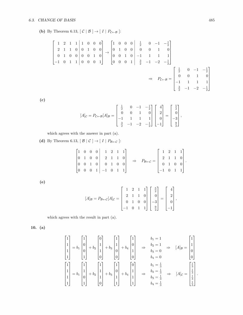
6.3. CHANGE OF BASIS 485
(b) By Theorem 6.13, [ C | B ]→ [ I | PC←B ]:
1 2 1 1 1 0 0 0
2 1 1 0 0 1 0 0
0 1 0 0 0 0 1 0
−1 0 1 1 0 0 0 1
→
1 0 0 0 12 0 −1 − 1
2
0 1 0 0 0 0 1 0
0 0 1 0 −1 1 1 1
0 0 0 1 32 −1 −2 − 1
2
⇒ PC←B =
12 0 −1 − 1
2
0 0 1 0
−1 1 1 132 −1 −2 − 1
2
(c)
[A]C = PC←B[A]B =
12 0 −1 − 1
2
0 0 1 0
−1 1 1 132 −1 −2 − 1
2
4
2
0
−1
=
52
0
−392
,which agrees with the answer in part (a).
(d) By Theorem 6.13, [ B | C ]→ [ I | PB←C ]:1 0 0 0 1 2 1 1
0 1 0 0 2 1 1 0
0 0 1 0 0 1 0 0
0 0 0 1 −1 0 1 1
⇒ PB←C =
1 2 1 1
2 1 1 0
0 1 0 0
−1 0 1 1
.
(e)
[A]B = PB←C [A]C =
1 2 1 1
2 1 1 0
0 1 0 0
−1 0 1 1
52
0
−392
=
4
2
0
−1
,
which agrees with the result in part (a).
10. (a) 1
1
1
1
= b1
1
0
0
1
+ b2
0
1
1
0
+ b3
1
1
0
0
+ b4
1
0
1
0
⇒
b1 = 1
b2 = 1
b3 = 0
b4 = 0
⇒ [A]B =
1
1
0
0
1
1
1
1
= b1
1
1
0
1
+ b2
1
1
1
0
+ b3
1
0
1
1
+ b4
0
1
1
1
⇒
b1 = 13
b2 = 13
b3 = 13
b4 = 13
⇒ [A]C =
13131313
.

486 CHAPTER 6. VECTOR SPACES
(b) By Theorem 6.13, [ C | B ]→ [ I | PC←B ]:
1 1 1 0 1 0 1 1
1 1 0 1 0 1 1 0
0 1 1 1 0 1 0 1
1 0 1 1 1 0 0 0
→
1 0 0 0 23 − 1
323 − 1
3
0 1 0 0 − 13
23
23
23
0 0 1 0 23 − 1
3 − 13
23
0 0 0 1 − 13
23 − 1
3 − 13
⇒ PC←B =
23 − 1
323 − 1
3
− 13
23
23
23
23 − 1
3 − 13
23
− 13
23 − 1
3 − 13
.
(c)
[A]C = PC←B[A]B =
23 − 1
323 − 1
3
− 13
23
23
23
23 − 1
3 − 13
23
− 13
23 − 1
3 − 13
1
1
0
0
=
13131313
which agrees with the answer in part (a).
(d) By Theorem 6.13, [ B | C ]→ [ I | PB←C ]:
1 0 1 1 1 1 1 0
0 1 1 0 1 1 0 1
0 1 0 1 0 1 1 1
1 0 0 0 1 0 1 1
→
1 0 0 0 1 0 1 1
0 1 0 0 12
12
12
32
0 0 1 0 12
12 − 1
2 − 12
0 0 0 1 − 12
12
12 − 1
2
⇒ PB←C =
1 0 1 112
12
12
32
12
12 − 1
2 − 12
− 12
12
12 − 1
2
.
(e)
[A]B = PB←C [A]C =
1 0 1 112
12
12
32
12
12 − 1
2 − 12
− 12
12
12 − 1
2
13131313
=
1
1
0
0
which agrees with the result in part (a).
11. Note that in terms of the standard basis {sinx, cosx},
B =
{[11
],
[01
]}, C =
{[11
],
[1−1
]}.

6.3. CHANGE OF BASIS 487
(a)
2 sinx− 3 cosx = b1(sinx+ cosx) + b2(cosx) ⇒ b1 = 2
b2 = −5
⇒ [2 sinx− 3 cosx]B =
[2
−5
]
2 sinx− 3 cosx = c1(sinx+ cosx) + c2(sinx− cosx) ⇒ c1 = − 12
c2 = 52
⇒ [2 sinx− 3 cosx]C =
[− 1
252
].
(b) By Theorem 6.13, [ C | B ]→ [ I | PC←B ]:[1 1 1 0
1 −1 1 1
]→
[1 0 1 1
2
0 1 0 − 12
]⇒ PC←B =
[1 1
2
0 − 12
].
(c) [2 sinx − 3 cosx]C = PC←B[2 sinx − 3 cosx]B =
[1 1
2
0 − 12
][2
−5
]=
[− 1
252
], which agrees with the
answer in part (a).
(d) By Theorem 6.13, [ B | C ]→ [ I | PB←C ]:[1 0 1 11 1 1 −1
]→[1 0 1 10 1 0 −2
]⇒ PC←B =
[1 10 −2
]
(e) [2 sinx − 3 cosx]B = PB←C [2 sinx − 3 cosx]C =
[1 1
0 −2
][− 1
252
]=
[2
−5
], which agrees with the
answer in part (a).
12. Note that in terms of the standard basis {sinx, cosx},
B =
{[11
],
[01
]}, C =
{[−1
1
],
[11
]}.
(a)
sinx = b1(sinx+ cosx) + b2(cosx) ⇒b1 = 1
b2 = −1⇒ [sinx]B =
[1
−1
]
sinx = c1(cosx− sinx) + c2(sinx+ cosx) ⇒c1 = − 1
2
c2 = 12
⇒ [sinx]C =
[− 1
212
]
(b) By Theorem 6.13, [ C | B ]→ [ I | PC←B ]:[−1 1 1 0
1 1 1 1
]→
[1 0 0 1
2
0 1 1 12
]⇒ PC←B =
[0 1
2
1 12
].
(c) [sinx]C = PC←B[sinx]B =
[0 1
2
1 12
][1
−1
]=
[− 1
212
], which agrees with the answer in part (a).

488 CHAPTER 6. VECTOR SPACES
(d) By Theorem 6.13, [ B | C ]→ [ I | PB←C ]:[1 0 −1 11 1 1 1
]→[1 0 −1 10 1 2 0
]⇒ PC←B =
[−1 1
2 0
]
(e) [sinx]B = PB←C [sinx]C =
[−1 1
2 0
][− 1
212
]=
[1
−1
], which agrees with the answer in part (a).
13. From Section 3.6, Example 3.58, if B is the usual basis and C is the basis whose basis vectors are therotations of the usual basis vectors through 60◦, the matrix of the rotation is
PC←B =
[cos 60◦ sin 60◦
− sin 60◦ cos 60◦
]=
[12
√3
2
−√
32
12
].
Then
(a)
[x]C = PC←B[x]B =
[12
√3
2
−√
32
12
][3
2
]=
[32 +√
3
1− 32
√3
].
(b) Since PC←B is an orthogonal matrix, we have
[x]B = (PC←B)−1
[x]C = (PC←B)T
[x]C =
[12 −
√3
2√3
212
][4
−4
]=
[2√
3 + 2
2√
3− 2
].
14. From Section 3.6, Example 3.58, if B is the usual basis and C is the basis whose basis vectors are therotations of the usual basis vectors through 135◦, the matrix of the rotation is
PC←B =
[cos 135◦ sin 135◦
− sin 135◦ cos 135◦
]=
[−√
22
√2
2
−√
22 −
√2
2
].
Then
(a)
[x]C = PC←B[x]B =
[−√
22
√2
2
−√
22 −
√2
2
][3
2
]=
[−√
22
− 5√
22
].
(b) Since PC←B is an orthogonal matrix, we have
[x]B = (PC←B)−1
[x]C = (PC←B)T
[x]C =
[−√
22 −
√2
2√2
2 −√
22
][4
−4
]=
[0
4√
2
].
15. By definition, the columns of PC←B are the coordinates of B in the basis C, so we have
[u1]C =
[1−1
], so that u1 = 1
[12
]− 1
[23
]=
[−1−1
][u2]C =
[−1
2
], so that u2 = −1
[12
]+ 2
[23
]=
[34
].
Therefore
B = {u1,u2} =
{[−1−1
],
[34
]}.

6.3. CHANGE OF BASIS 489
16. Let C = {p1(x), p2(x), p3(x)}. By definition, the columns of PC←B are the coordinates of B in the basisC, so that
[x]C =
10−1
⇒ x = p1(x)− p3(x),
[1 + x]C =
021
⇒ 1 + x = 2p2(x) + p3(x),
[1− x+ x2]C =
011
⇒ 1− x+ x2 = p2(x) + p3(x).
Subtract the third equation from the second, giving p2(x) = 2x− x2; substituting back into the thirdequation gives p3(x) = 1− 3x+ 2x2; then from the first equation, p1(x) = 1− 2x+ 2x2. So
C = {p1(x), p2(x), p3(x)} = {1− 2x+ 2x2, 2x− x2, 1− 3x+ 2x2}.
17. Since a = 1 in this case and we are considering a quadratic, we have for the Taylor basis of P2
B = {1, x− 1, (x− 1)2} = {1, x− 1, x2 − 2x+ 1}.
Let C = {1, x, x2} be the standard basis for P2. Then
[p(x)]C =
12−5
.To find the change-of-basis matrix PB←C , we reduce
[B C
]→[I PB←C
]:
[B C
]=
1 −1 1 1 0 00 1 −2 0 1 00 0 1 0 0 1
→1 0 0 1 1 1
0 1 0 0 1 20 0 1 0 0 1
.Therefore
[p(x)]C = PB←C [p(x)]B =
1 1 10 1 20 0 1
12−5
=
−2−8−5
,so that the Taylor polynomial centered at 1 is
−2− 8(x− 1)− 5(x− 1)2.
18. Since a = −2 in this case and we are considering a quadratic, we have for the Taylor basis of P2
B = {1, x+ 2, (x+ 2)2} = {1, x+ 2, x2 + 4x+ 4}.
Let C = {1, x, x2} be the standard basis for P2. Then
[p(x)]C =
12−5
.To find the change-of-basis matrix PB←C , we reduce
[B C
]→[I PB←C
]:
[B C
]=
1 2 4 1 0 00 1 4 0 1 00 0 1 0 0 1
→1 0 0 1 −2 4
0 1 0 0 1 −40 0 1 0 0 1
.

490 CHAPTER 6. VECTOR SPACES
Therefore
[p(x)]C = PB←C [p(x)]B =
1 −2 40 1 −40 0 1
12−5
=
−2322−5
,so that the Taylor polynomial centered at −2 is
−23 + 22(x+ 2)− 5(x+ 2)2.
19. Since a = −1 in this case and we are considering a cubic, we have for the Taylor basis of P3
B = {1, x+ 1, (x+ 1)2, (x+ 1)3} = {1, x+ 1, x2 + 2x+ 1, x3 + 3x2 + 3x+ 1}.
Let C = {1, x, x2, x3} be the standard basis for P2. Then
[p(x)]C =
0001
.To find the change-of-basis matrix PB←C , we reduce
[B C
]→[I PB←C
]:
[B C
]=
1 1 1 1 1 0 0 00 1 2 3 0 1 0 00 0 1 3 0 0 1 00 0 0 1 0 0 0 1
→
1 0 0 0 1 −1 1 −10 1 0 0 0 1 −2 30 0 1 0 0 0 1 −30 0 0 1 0 0 0 1
.Therefore
[p(x)]C = PB←C [p(x)]B =
1 −1 1 −10 1 −2 30 0 1 −30 0 0 1
0001
=
−1
3−3
1
,so that the Taylor polynomial centered at −1 is
−1 + 3(x+ 1)− 3(x+ 1)2 + (x+ 1)3.
20. Since a = 12 in this case and we are considering a cubic, we have for the Taylor basis of P3
B =
{1, x− 1
2,
(x− 1
2
)2
,
(x− 1
2
)3}
=
{1, x− 1
2, x2 − x+
1
4, x3 − 3
2x2 +
3
4x− 1
8
}.
Let C = {1, x, x2, x3} be the standard basis for P2. Then
[p(x)]C =
0001
.To find the change-of-basis matrix PB←C , we reduce
[B C
]→[I PB←C
]:
[B C
]=
1 − 1
214 − 1
8 1 0 0 0
0 1 −1 34 0 1 0 0
0 0 1 − 32 0 0 1 0
0 0 0 1 0 0 0 1
→
1 0 0 0 1 12
14
18
0 1 0 0 0 1 1 34
0 0 1 0 0 0 1 32
0 0 0 1 0 0 0 1
.
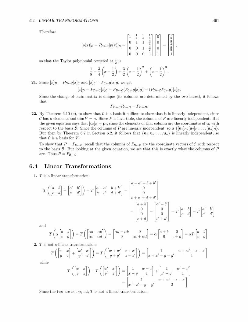
6.4. LINEAR TRANSFORMATIONS 491
Therefore
[p(x)]C = PB←C [p(x)]B =
1 1
214
18
0 1 1 34
0 0 1 32
0 0 0 1
0
0
0
1
=
183432
1
,so that the Taylor polynomial centered at 1
2 is
1
8+
3
4
(x− 1
2
)+
3
2
(x− 1
2
)2
+
(x− 1
2
)3
.
21. Since [x]D = PD←C [x]C and [x]C = PC←B[x]B, we get
[x]D = PD←C [x]C = PD←C(PC←B[x]B) = (PD←CPC←B)[x]B.
Since the change-of-basis matrix is unique (its columns are determined by the two bases), it followsthat
PD←CPC←B = PD←B.
22. By Theorem 6.10 (c), to show that C is a basis it suffices to show that it is linearly independent, sinceC has n elements and dimV = n. Since P is invertible, the columns of P are linearly independent. Butthe given equation says that [ui]B = pi, since the elements of that column are the coordinates of ui withrespect to the basis B. Since the columns of P are linearly independent, so is {[u1]B, [u2]B, . . . , [un]B}.But then by Theorem 6.7 in Section 6.2, it follows that {u1,u2, . . . ,un} is linearly independent, sothat C is a basis for V .
To show that P = PB←C , recall that the columns of PB←C are the coordinate vectors of C with respectto the basis B. But looking at the given equation, we see that this is exactly what the columns of Pare. Thus P = PB←C .
6.4 Linear Transformations
1. T is a linear transformation:
T
([a bc d
]+
[a′ b′
c′ d′
])= T
[a+ a′ b+ b′
c+ c′ d+ d′
]=
a+ a′ + b+ b′
00
c+ c′ + d+ d′
=
a+ b
00
c+ d
+
a′ + b′
00
c′ + d′
= T
[a bc d
]+ T
[a′ b′
c′ d′
]
and
T
(α
[a bc d
])= T
([αa αbαc αd
])=
[αa+ αb 0
0 αc+ αd
]= α
[a+ b 0
0 c+ d
]= αT
[a bc d
].
2. T is not a linear transformation:
T
([w xy z
]+
[w′ x′
y′ z′
])= T
([w + w′ x+ x′
y + y′ z + z′
])=
[1 w + w′ − z − z′
x+ x′ − y − y′ 1
]while
T
([w xy z
])+ T
([w′ x′
y′ z′
])=
[1 w − z
x− y 1
]+
[1 w′ − z′
x′ − y′ 1
]=
[2 w + w′ − z − z′
x+ x′ − y − y′ 2
]Since the two are not equal, T is not a linear transformation.

492 CHAPTER 6. VECTOR SPACES
3. T is a linear transformation. If A,C ∈Mnn and α is a scalar, then
T (A+ C) = (A+ C)B = AB + CB = T (A) + T (C)
T (αA) = (αA)B = α(AB) = αT (A).
4. T is a linear transformation. If A,C ∈Mnn and α is a scalar, then
T (A+ C) = (A+ C)B −B(A+ C) = AB + CB −BA−BC = (AB −BA) + (CB −BC)
= T (A) + T (C)
T (αA) = (αA)B −B(αA) = α(AB)− α(BA) = α(AB −BA) = αT (A).
5. T is a linear transformation, since by Exercise 44 in Section 3.2, tr(A + B) = tr(A) + tr(B) andtr(αA) = α tr(A).
6. T is not a linear transformation. For example, in M22, let A = I; then T (2A) = T (2I) = 2 · 2 = 4,while 2T (A) = 2T (I) = 2(1 · 1) = 2.
7. T is not a linear transformation. For example, let A be any invertible matrix in Mnn; then −A isinvertible as well, so that rank(A) = rank(−A) = n. Then
T (A) + T (−A) = rank(A) + rank(−A) = 2n while T (A+ (−A)) = T (O) = rank(O) = 0.
8. Since T (0) = 1 + x+ x2 6= 0, T is not a linear transformation by Theorem 6.14(a).
9. T is a linear transformation. Let p(x) = a + bx + cx2 and p′(x) = a′ + b′x + c′x2 be elements of P2,and let α be a scalar. Then
(T (p+ p′))(d) = (T ((a+ a′) + (b+ b′)x+ (c+ c′)x2))(d)
= (a+ a′) + (b+ b′)(d+ 1) + (b+ b′)(d+ 1)2
=(a+ b(d+ 1) + b(d+ 1)2
)+(a′ + b′(d+ 1) + b′(d+ 1)2
)= (T (p))(d) + (T (p′))(d),
and
T (αp)(d) = (T (αa+ αbx+ αcx2))(d) = αa+ αb(d+ 1) + αb(d+ 1)2
= α(a+ b(d+ 1) + b(d+ 1)2
)= α(T (p))(d).
10. T is a linear transformation. Let f, g ∈ F and α be a scalar. Then
(T (f + g))(x) = (f + g)(x2) = f(x2) + g(x2) = (T (f))(x) + (T (g))(x)
(T (αf))(x) = (αf)(x2) = αf(x2) = α(T (f))(x).
11. T is not a linear transformation. For example, let f be any function in F that takes on a value otherthan 0 or 1. Then
(T (2f))(x) = ((2f)(x))2
= (2f(x))2
= 4f(x)2 6= 2f(x)2 = 2(T (f))(x),
where the inequality holds because of the conditions on f .
12. This is similar to Exercise 10; T is a linear transformation. Let f, g ∈ F and α be a scalar. Then
(T (f + g))(c) = (f + g)(c) = f(c) + g(c) = (T (f))(c) + (T (g))(c)
(T (αf))(c) = (αf)(c) = αf(c) = α(T (f))(c)

6.4. LINEAR TRANSFORMATIONS 493
13. For T , we have (with α a scalar)
T
([ab
]+
[cd
])= T
[a+ cb+ d
]= (a+ c) + (a+ c+ b+ d)x = (a+ (a+ b)x) + (c+ (c+ d)x)
= T
[ab
]+ T
[cd
]T
(α
[ab
])= T
[αaαb
]= αa+ (αa+ αb)x = α(a+ (a+ b)x) = αT
[ab
].
For S, suppose that p(x), q(x) ∈P1 and α is a scalar; then
T (p(x) + q(x)) = x(p(x) + q(x)) = xp(x) + xq(x) = T (p(x)) + T (q(x))
T (αp(x)) = x(αp(x)) = α(xp(x)) = αT (p(x)).
14. Using the comment following the definition of a linear transformation, we have
T
[52
]= T
(5
[10
]+ 2
[01
])= 5T
[10
]+ 2T
[01
]= 5
12−1
+ 2
304
=
510−5
+
608
=
11103
In a similar way,
T
[ab
]= T
(a
[10
]+ b
[01
])= aT
[10
]+ bT
[01
]= a
12−1
+ b
304
=
a2a−a
+
3b0
4b
=
a+ 3b2a
−a+ 4b
15. We must first find the coordinates of
[−7
9
]in the basis
{[11
],
[3−1
]}. So we want to find c, d such
that [−7
9
]= c
[11
]+ d
[3−1
]⇒ c + 3d = −7
c − d = 9⇒ c = 5
d = −4.
Then using the comment following the definition of a linear transformation, we have
T
[−7
9
]= T
(5
[11
]− 4
[3−1
])= 5T
[11
]− 4T
[3−1
]= 5(1− 2x)− 4(x+ 2x2) = −8x2 − 14x+ 5.
The second part is much the same, except that we need to find c, d such that[ab
]= c
[11
]+ d
[3−1
]⇒ c + 3d = a
c − d = b⇒
c = a+3b4
d = a−b4 .
Then using the comment following the definition of a linear transformation, we have
T
[ab
]= T
(a+ 3b
4
[11
]+a− b
4
[3−1
])=a+ 3b
4T
[11
]+a− b
4T
[3−1
]=a+ 3b
4(1− 2x) +
a− b4
(x+ 2x2)
=a− b
2x2 − a+ 7b
4x+
a+ 3b
4.
16. Since T is linear,
T (6 + x− 4x2) = T (6) + T (x) + T (−4x2) = 6T (1) + T (x)− 4T (x2)
= 6(3− 2x) + (4x− x2)− 4(2 + 2x2) = 10− 8x− 9x2.

494 CHAPTER 6. VECTOR SPACES
Similarly,
T (a+ bx+ cx2) = T (a) + T (bx) + T (cx2) = aT (1) + bT (x) + cT (x2)
= a(3− 2x) + b(4x− x2) + c(2 + 2x2) = (3a+ 2c) + (4b− 2a)x+ (2c− b)x2.
17. We do the second part first, then substitute for a, b, and c to get the first part. We must find thecoordinates of a+ bx+ cx2 in the basis
{1 + x, x+ x2, 1 + x2
}. So we want to find r, s, t such that
a+ bx+ cx2 = r(1 + x) + s(x+ x2) + t(1 + x2) = (r + t) + (r + s)x+ (s+ t)x2 ⇒
r + t = ar + s = b
s + t = c⇒
r = a+b−c2
s = −a+b+c2
t = a−b+c2 .
Then using the comment following the definition of a linear transformation, we have
T (a+ bx+ cx2) = T
(a+ b− c
2(1 + x) +
−a+ b+ c
2(x+ x2) +
a− b+ c
2(1 + x2)
)=a+ b− c
2T (1 + x) +
−a+ b+ c
2T (x+ x2) +
a− b+ c
2T (1 + x2)
=a+ b− c
2(1 + x2) +
−a+ b+ c
2(x− x2) +
a− b+ c
2(1 + x+ x2)
= a+ cx+3a− b− c
2x2
For the second part, substitute a = 4, b = −1, and c = 3 to get
T (4− x+ 3x2) = 4 + 3x+12 + 1− 3
2x2 = 4 + 3x+ 5x2.
18. We do the second part first, then substitute for a, b, c, and d to get the first part. We must find thecoordinates of [
a bc d
]in the basis
[1 00 0
],
[1 10 0
],
[1 11 0
],
[1 11 1
].
So we want to find r, s, t, u such that
[a bc d
]= r
[1 00 0
]+ s
[1 10 0
]+ t
[1 11 0
]+ u
[1 11 1
]⇒
r + s + t + u = as + t + u = b
t + u = cu = d
⇒
r = a− bs = b− ct = c− du = d.
Then using the comment following the definition of a linear transformation, we have
T
[a bc d
]= T
((a− b)
[1 00 0
]+ (b− c)
[1 10 0
]+ (c− d)
[1 11 0
]+ +d
[1 11 1
])= (a− b)T
[1 00 0
]+ (b− c)T
[1 10 0
]+ (c− d)T
[1 11 0
]+ +dT
[1 11 1
]= (a− b) · 1 + (b− c) · 2 + (c− d) · 3 + d · 4= a+ b+ c+ d.
For the second part, substitute a = 1, b = 3, c = 4, d = 2 to get
T
[1 34 2
]= 1 + 3 + 4 + 2 = 10.

6.4. LINEAR TRANSFORMATIONS 495
19. LetT (E11) = a, T (E12) = b, T (E21) = c, T (E22) = d.
Then
T
[w xy z
]= t (wE11 + xE12 + yE21 + zE22) = wTE11 +xTE12 +yTE21 + zTE22 = aw+ bx+ cy+dz.
20. Writing 06−8
= a
210
+ b
302
means that we must have b = −4, and then a = 6, so that if T were a linear transformation, then
T
06−8
= 6T
210
− 4
302
= 6(1 + x)− 4(2− x+ x2) = −2 + 10x− 4x2 6= −2 + 2x2.
This is a contradiction, so T cannot be linear.
21. Choose v ∈ V . Then −v = 0 − v by definition, so using part (a) of Theorem 6.14 and the definitionof a linear transformation,
T (−v) = T (0− v) = T (0)− T (v) = 0− T (v) = −T (v).
22. Choose v ∈ V . Then there are scalars c1, . . . , cn such that v =∑ni=1 civi since the vi are a basis.
Since T is linear, using the comment following the definition of a linear transformation we get
T (v) = T
(n∑i=1
civi
)=
n∑i=1
ciT (vi) =
n∑i=1
civi = v.
Since T (v) = v for every vector v ∈ V , T is the identity transformation.
23. We must show that if p(x) ∈Pn, then Tp(x) = p′(x). Suppose that p(x) =∑nk=0 akx
k. Then since Tis linear, using the comment following the definition of a linear transformation we get
Tp(x) = T
(n∑k=0
akxk
)=
n∑k=0
akT (xk) = a0T (1) +
n∑k=1
akT (xk) =
n∑k=1
kakxk−1 = p′(x).
24. (a) We prove the contrapositive: suppose that {v1, . . . ,vn} is linearly dependent in V ; then we have
c1v1 + · · ·+ cnvn = 0,
where not all of the ci are zero. Then
T (c1v1 + · · ·+ cnvn) = c1T (v1) + · · ·+ cnT (vn) = T (0) = 0,
showing that {T (v1), . . . , T (vn)} is linearly dependent in W . Therefore if {T (v1), . . . , T (vn)} islinearly independent in W , we must also have that {v1, . . . ,vn} is linearly independent in V .
(b) For example, the zero transformation from V to W , which takes every element of V to 0, showsthat the converse is false. There are many other examples as well, however. For instance, let
T : R2 → R2 :
[xy
]7→[x0
].
Then e1 and e2 are linearly independent in V , but
T (e1) =
[10
]and T (e2) =
[00
]are linearly dependent.

496 CHAPTER 6. VECTOR SPACES
25. We have
(S ◦ T )
[21
]= S
(T
[21
])= S
[5−1
]=
[4 −10 6
](S ◦ T )
[xy
]= S
(T
[xy
])= S
[2x+ y−y
]=
[2x −y0 2x+ 2y
].
Since the domain of T is R2 but the codomain of S is M22, T ◦ S does not make sense and we cannotcompute it.
26. We have
(S ◦ T )(3 + 2x− x2) = S(T (3 + 2x− x2)) = S(2 + 2 · (−1)x) = S(2− 2x)
= 2 + (2− 2)x+ 2 · (−2)x2 = 2− 4x2
(S ◦ T )(a+ bx+ cx2) = S(T (a+ bx+ cx2)) = S(b+ 2cx) = b+ (b+ 2c)x+ 2(2c)x2
= b+ (b+ 2c)x+ 4cx2.
Since the domain of S is P1, which equals the codomain of T , we can compute T ◦ S:
(T ◦ S)(a+ bx) = T (S(a+ bx)) = T (a+ (a+ b)x+ 2bx2) = (a+ b) + 2 · 2bx = (a+ b) + 4bx.
27. The Chain Rule says that (f ◦ g)′(x) = g′(x)f ′(g(x)). Let g(x) = x+ 1 and f(x) = p(x). Then
(S ◦ T )(p(x)) = S(T (p(x))) = S(p′(x)) = p′(x+ 1)
(T ◦ S)(p(x)) = T (S(p(x))) = T (p(x+ 1)) = T ((p ◦ g)(x)) = (p ◦ g)′(x) = g′(x)p′(g(x)) = p′(x+ 1)
since the derivative of g(x) is 1.
28. Use the Chain Rule from the previous exercise, and let g(x) = x+ 1:
(S ◦ T )(p(x)) = S(T (p(x))) = S(xp′(x)) = (x+ 1)p′(x+ 1)
(T ◦ S)(p(x)) = T (S(p(x))) = T (p(x+ 1)) = T ((p ◦ g)(x)) = x(p ◦ g)′(x) = xg′(x)p′(g(x)) = xp′(x+ 1)
since the derivative of g(x) is 1.
29. We must verify that S ◦ T = IR2 and T ◦ S = IR2 .
(S ◦ T )
[xy
]= S
(T
[xy
])= S
[x− y−3x+ 4y
]=
[4(x− y) + (−3x+ 4y)3(x− y) + (−3x+ 4y)
]=
[xy
](T ◦ S)
[xy
]= T
(S
[xy
])= T
[4x+ y3x+ y
]=
[(4x+ y)− (3x+ y)−3(4x+ y) + 4(3x+ y)
]=
[xy
].
Thus (S ◦ T )
[xy
]= (T ◦ S)
[xy
]=
[xy
]for any vector
[xy
], so both compositions are the identity and
we are done.
30. We must verify that S ◦ T = IP1 and T ◦ S = IP1 .
(S ◦ T )(a+ bx) = S(T (a+ bx)) = S
(b
2+ (a+ 2b)x
)=
(−4 · b
2+ (a+ 2b)
)+ 2 · b
2x = a+ bx
(T ◦ S)(a+ bx) = T (S(a+ bx)) = T ((−4a+ b) + 2ax) =2a
2+ ((−4a+ b) + 2 · 2a)x = a+ bx.
Thus (S ◦ T )(a + bx) = (T ◦ S)(a + bx) = a + bx for any a + bx ∈ P1, so both compositions are theidentity and we are done.

6.4. LINEAR TRANSFORMATIONS 497
31. Suppose T ′ and T ′′ are such that T ′ ◦ T = T ′′ ◦ T = IV and T ◦ T ′ = T ◦ T ′′ = IW . To show thatT ′ = T ′′, it suffices to show that T ′(w) = T ′′(w) for any vector w ∈W . But
T ′(w) = IV ◦ T ′(w) = T ′′ ◦ T ◦ T ′(w) = T ′′ ◦ ((T ◦ T ′)w) = T ′′ ◦ IW (w) = T ′′(w).
32. (a) First, if T (v) = ±v, then clearly {v, Tv} is linearly dependent. For the converse, if {v, T (v)} islinearly dependent, then for some c, d not both zero cv + dTv = 0. Then
T (cv + dTv) = cTv + d(T ◦ T )v = cTv + dv = T0 = 0
since T ◦ T = IV . Thus
cv + dTv = 0
cTv + dv = 0.
Subtracting these two equations gives c(Tv − v) − d(Tv − v) = (c − d)(Tv − v) = 0. But thismeans that either c = d 6= 0 or that Tv = v. If c = d 6= 0, then divide through by c in theequation cv + dTv = 0 to get v + Tv = 0, so that Tv = −v. Hence Tv = ±v.
(b) Let T
[xy
]=
[−x−y
]. Then
(T ◦ T )
[xy
]= T
(T
[xy
])= T
[−x−y
]=
[−(−x)−(−y)
]=
[xy
],
so that T ◦ T = IV , and
[xy
]and
[−x−y
]are linearly dependent.
33. (a) First, if T (v) = v, then clearly {v, Tv} = {v,v} is linearly dependent, and if T (v) = 0, then{v, Tv} = {v,0} is linearly dependent. For the converse, suppose that {v, Tv} is linearly depen-dent. Then there exist c, d, not both zero, such that
cv + dTv = 0.
As in Exercise 32, we get
T (cv + dTv) = cTv + d(T ◦ T )v = cTv + dTv = T0 = 0
since T ◦ T = T . Thus
(c+ d)Tv = 0
cv + dTv = 0.
Subtracting the two equations gives c(v− Tv) = 0, so that either Tv = v or c = 0. But if c = 0,then cv + dTv = dTv = 0, so that since c and d were not both zero, d cannot be zero, so thatTv = 0. Thus either Tv = v or Tv = 0.
(b) For example, let T
[xy
]=
[x0
]. This is a projection operator, so we already know that T ◦ T = T ;
to show this via computation,
(T ◦ T )
[xy
]= T
(T
[xy
])= T
[x0
]=
[x0
]= T
[xy
].
Then for example T
[10
]=
[10
]while T
[01
]= 0.

498 CHAPTER 6. VECTOR SPACES
34. To show that S+T is a linear transformation, we must show it obeys the rules of a linear transformation.Using the definition of S + T and of cT , as well as the fact that both S and T are linear, we have
(S + T )(u + v) = S(u + v) + T (u + v) = Su + Sv + Tu + Tv = (Su + Tu) + (Sv + Tv)
= (S + T )u + (S + T )v
(c(S + T ))v = (cS + cT )v = (cS)v + (cT )v = c(Sv) + c(Tv) = c(Sv + Tv) = c(S + T )v.
35. We show that L = L (V,W ) satisfies the ten axioms of a vector space. We use freely below the factthat V and W are both vector spaces. Also, note that S = T in L (V,W ) simply means that Sv = Tvfor all v ∈ V .
1. From Exercise 34, S, T ∈ L implies that S + T ∈ L .
2. (S + T )v = Sv + Tv = Tv + Sv = (T + S)v.
3. ((R+ S) + T )v = (R+ S)v + Tv = Rv + Sv + Tv = Rv + (S + T )v = (R+ (S + T ))v.
4. Let Z : V → W be the map Z(v) = 0 for all v ∈ V. Then Z is the zero map, so it is linear andthus in L , and
(S + Z)v = Sv + Zv = Sv + 0 = Sv.
5. If S ∈ L , let −S : V →W be the map (−S)v = −Sv. By Exercise 34, −S ∈ L , and
(S + (−S))v = Sv + (−S)v = Sv − Sv = 0.
6. By Exercise 34, if S ∈ L , then cS ∈ L .
7. (c(S + T ))v = c(S + T )v = c(Sv + Tv) = cSv + cTv = (cS)v + (cT )v = ((cS) + (cT ))v.
8. ((c+ d)S)v = (c+ d)Sv = cSv + dSv = (cS)v + (cT )v = ((cS) + (cT ))v.
9. (c(dS))v = c(dS)v = c(dSv) = (cd)Sv = ((cd)S)v.
10. By Exercise 34, (1S)v = 1Sv = Sv.
36. To show that these linear transformations are equal, it suffices to show that they have the same valueon every element of V .
(a) (R ◦ (S + T ))v = R((S + T )v) = R(Sv + Tv) = R(Sv) +R(Tv) = (R ◦ S)v + (R ◦ T )v.
(b)
(c(R ◦ S))v = c(R ◦ S)v = cR(Sv) = (cR)(Sv) = ((cR) ◦ S)v
(c(R ◦ S))v = c(R ◦ S)v = cR(Sv) = (cR)(Sv) = R((cS)v) = (R ◦ (cS))v.
6.5 The Kernel and Range of a Linear Transformation
1. (a) Only (ii) is in ker(T ), since
(i) T
[1 2−1 3
]=
[1 00 3
]6= O,
(ii) T
[0 42 0
]=
[0 00 0
]= O,
(iii) T
[3 00 −3
]=
[3 00 −3
]6= O.
(b) From the definition of T , a matrix is in range(T ) if and only if its two off-diagonal elements arezero. Thus only (iii) is in range(T ).
2. (a) T is explicitly defined by
T
[a bc d
]= a+ d
Thus

6.5. THE KERNEL AND RANGE OF A LINEAR TRANSFORMATION 499
(i) T
[1 2−1 3
]= 1 + 3 = 4
(ii) T
[0 42 0
]= 0 + 0 = 0
(iii) T
[1 30 −1
]= 1 + (−1) = 0,
and therefore (ii) and (iii) are in ker(T ) but (i) is not.
(b) All three of these are in range(T ). For example,
(i) T
[0 00 0
]= 0 + 0 = 0,
(ii) T
[2 14 0
]= 2 + 0 = 2,
(iii) T
[√2
2 π12 0
]=√
22 + 0 =
√2
2 .
(c) ker(T ) is the set of all matrices in M22 whose diagonal elements are negatives of each other.range(T ) is all real numbers.
3. (a) We have
(i) T (1 + x) = T (1 + 1x+ 0x2) =
[1− 11 + 0
]=
[01
]6= 0,
(ii) T (x− x2) = T (0 + 1x− 1x2) =
[0− 1
1 + (−1)
]=
[−1
0
]6= 0,
(iii) T (1 + x− x2) = T (1 + 1x− 1x2) =
[1− 1
1 + (−1)
]=
[00
]= 0,
so only (iii) is in range(T ).
(b) All of them are. For example,
(i) T (1 + x− x2) =
[00
], from part (a),
(ii) T (1) =
[1− 00 + 0
]=
[10
],
(iii) T (x2) =
[0− 00 + 1
]=
[01
].
(c) ker(T ) consists of all polynomials a + bx + cx2 such that a = b and b = −c; parametrizing viaa = t gives ker(T ) = {a+ax−ax2}, so that ker(T ) consists of all multiples of 1+x−x2. range(T )is all of R2, since it is a subspace of R2 containing both e1 and e2 (see items (ii) and (iii) of part(b)).
4. (a) Since xp′(x) = 0 if and only if p′(x) = 0, we see that only (i) is in ker(T ). For the other two, wehave T (x) = xx′ = x and T (x2) = x(x2)′ = 2x2.
(b) A polynomial in range(T ) must be divisible by x; that is, it must have no constant term. Thus(i) is not in range(T ). However, x = T (x) from part (a), and also from part (a), we see thatT(
12x
2)
= x2. Thus (ii) and (iii) are in range(T ).
(c) ker(T ) consists of all polynomials whose derivative vanishes, so it consists of constant polynomials.range(T ) consists of all polynomials with zero constant terms, since given any such polynomial,we may write it as xg(x) for some polynomial g(x); then clearly T
(∫g(x) dx
)= xg(x).
5. Since ker(T ) =
{[0 bc 0
]}, a basis for ker(T ) is
{[0 10 0
],
[0 01 0
]}.

500 CHAPTER 6. VECTOR SPACES
Similarly, since range(T ) =
{[a 00 d
]}, a basis for range(T ) is
{[1 00 0
],
[0 00 1
]}.
Thus dim ker(T ) = 2 and dim range(T ) = 2. The Rank Theorem says that
4 = dimM22 = nullity(T ) + rank(T ) = dim ker(T ) + dim range(T ) = 2 + 2,
which is true.
6. Since
ker(T ) =
{[a bc −a
]},
a basis for ker(T ) is {[1 00 −1
],
[0 10 0
],
[0 01 0
]}.
From Exercise 2, range(T ) = R. Thus dim ker(T ) = 3 and dim range(T ) = 1. The Rank Theorem saysthat
4 = dimM22 = nullity(T ) + rank(T ) = dim ker(T ) + dim range(T ) = 3 + 1,
which is true.
7. Since ker(T ) ={a+ ax− ax2
}, a basis for ker(T ) is {1 + x − x2}. From Exercise 3, range(T ) = R2.
Thus dim ker(T ) = 1 and dim range(T ) = 2. The Rank Theorem says that
3 = dim P2 = nullity(T ) + rank(T ) = dim ker(T ) + dim range(T ) = 1 + 2,
which is true.
8. Since ker(T ) is the constant polynomials, it has a basis {1}. From Exercise 4, range(T ) is the set ofpolynomials with nonzero constant terms, or {bx+cx2}, so it has a basis {x, x2}. Thus dim ker(T ) = 1and dim range(T ) = 2. The Rank Theorem says that
3 = dim P2 = nullity(T ) + rank(T ) = dim ker(T ) + dim range(T ) = 1 + 2,
which is true.
9. Since
T
[1 00 0
]=
[1− 00− 0
]=
[10
], T
[0 01 0
]=
[0− 01− 0
]=
[01
],
it follows that range(T ) = R2, since it is a subspace of R2 containing both e1 and e2. Thus rank(T ) =dim range(T ) = 2, so that by the Rank Theorem,
nullity(T ) = dimM22 − rank(T ) = 4− 2 = 2.
10. Since
T (1− x) =
[1− 01− 1
]=
[10
], T (x) =
[01
],
it follows that range(T ) = R2, since it is a subspace of R2 containing both e1 and e2. Thus rank(T ) =dim range(T ) = 2, so that by the Rank Theorem,
nullity(T ) = dim P2 − rank(T ) = 3− 2 = 1.

6.5. THE KERNEL AND RANGE OF A LINEAR TRANSFORMATION 501
11. If A =
[a bc d
], then
T (A) = AB =
[a bc d
] [1 −1−1 1
]=
[a− b −a+ bc− d −c+ d
]=
[a− b −(a− b)c− d −(c− d)
].
Thus T (A) = O if and only if a = b and c = d, so that
ker(T ) =
{[a ac c
]},
so that a basis for ker(T ) is {[1 10 0
],
[0 01 1
]}.
Hence nullity(T ) = dim ker(T ) = 2, so that by the Rank Theorem
rank(T ) = dimM22 − nullity(T ) = 4− 2 = 2.
12. If A =
[a bc d
], then
T (A) = AB −BA =
[a bc d
] [1 10 1
]−[1 10 1
] [a bc d
]=
[a a+ bc c+ d
]−[a+ c b+ dc d
]=
[−c a− d0 c
].
So A ∈ ker(T ) if and only if c = 0 and a = d, so that
A =
[a b0 a
]= a
[1 00 1
]+ b
[0 10 0
].
These two matrices are linearly independent since they are not multiples of one another, so thatnullity(T ) = 2. Since dimM22 = 4, we see that by the Rank Theorem
rank(T ) = dimM22 − nullity(T ) = 4− 2 = 2.
13. The derivative of p(x) = a + bx + cx2 is b + 2cx; then p′(0) = b, so this is zero if b = 0. Thusker(T ) = {a+ cx2}, so that a basis for ker(T ) is {1, x2}. Then nullity(T ) = dim ker(T ) = 2, so that bythe Rank Theorem,
rank(T ) = dim P2 − nullity(T ) = 3− 2 = 1.
14. We have
T (A) = A−AT =
0 a12 − a21 a13 − a31
a12 − a21 0 a23 − a32
a31 − a13 a32 − a23 0
,so that A ∈ ker(T ) if and only if a12 = a21, a13 = a31, and a23 = a32; that is, if and only if A issymmetric. By Exercise 40 in Section 6.2, nullity(T ) = dim ker(T ) = 3·4
2 = 6. Then by the RankTheorem,
rank(T ) = dimM33 − nullity(T ) = 9− 6 = 3.
15. (a) Yes, T is one-to-one. If
T
[ab
]=
[2a− ba+ 2b
]=
[00
],
then 2a− b = 0 and a+ 2b = 0. The only solution to this pair of equations is a = b = 0, so that
the only element of the kernel is
[00
]and thus T is one-to-one.
(b) Since T is one-to-one and the dimension of the domain and codomain are both 2, T must be ontoby Theorem 6.21.

502 CHAPTER 6. VECTOR SPACES
16. (a) Yes, T is one-to-one. If
T
[ab
]= (a− 2b) + (3a+ b)x+ (a+ b)x2 = 0,
then a + b = 0 from the third term. Since 3a + b = 0 as well, subtracting gives 2a = 0, so that
a = 0. The third term then forces b = 0. Thus
[ab
]= 0 and T is one-to-one.
(b) T cannot be onto. R2 has dimension 2, so by the rank theorem 2 = dimR2 = rank(T ) +nullity(T ) ≥ rank(T ). It follows that the dimension of the range of T is at most 2 (in fact, sincefrom part (a) nullity(T ) = 0, the dimension of the range is equal to 2). But dim P2 = 3, so T isnot onto.
17. (a) If T (a+ bx+ cx2) = 0, then
2a− b = 0
a+ b− 3c = 0
−a + c = 0.
Row-reducing the augmented matrix gives 2 −1 0 01 1 −3 0−1 0 1 0
→1 0 −1 0
0 1 −2 00 0 0 0
.This has nontrivial solutions a = t, b = 2t, c = t, so that
ker(T ) = {t+ 2tx+ tx2} = {t(1 + 2x+ x2)}.
So T is not one-to-one.
(b) Since dim P2 = dimR3 = 3, the fact that T is not one-to-one implies, by Theorem 6.21, that Tis not onto.
18. (a) By Exercise 10, nullity(T ) = 1, so that ker(T ) 6= {0}, so that T is not one-to-one.
(b) By Exercise 10, range(T ) = R2, so that T is onto by definition.
19. (a) If T
abc
= O, then a− b = a+ b = 0 and b− c = b+ c = 0; these equations give a = b = c = 0 as
the only solution. Thus T is one-to-one.
(b) By the Rank Theorem,
dim range(T ) = dimR3 − dim ker(T ) = 3− 0 = 3.
However, dimM22 = 4 > 3 = dim range(T ), so that T cannot be onto.
20. (a) If T
abc
= O, then a+ b+ c = 0, b− 2c = 0, and a− c = 0. The latter two equations give a = c
and b = 2c, so that from the first equation 4c = 0 and thus c = 0. It follows that a = b = 0. ThusT is one-to-one.
(b) By Exercise 40 in Section 6.2, dimW = 2·32 = 3 = dimR3. Since the dimensions of the domain
and codomain are equal and T is one-to-one, Theorem 6.21 implies that T is also onto.

6.5. THE KERNEL AND RANGE OF A LINEAR TRANSFORMATION 503
21. These vector spaces are isomorphic. Bases for the two vector spaces are
D3 : {E11, E22, E33}, R3 : {e1, e2, e3}.
Since both have dimension 3, we know that D3∼= R3. Define
T (aE11 + bE22 + cE33) = a e1 + b e2 + c e3.
Then T is a linear transformation from the way we have defined it. Since the ei are linearly independent,it follows that a e1 + b e2 + c e3 = 0 if and only if a = b = c = 0. Thus ker(T ) = {0} so that T isone-to-one. Since dimD3 = dimR3, we know that T is onto as well, so it is an isomorphism.
22. By Exercise 40 in Section 6.2, dimS3 = 3·42 = 6. Since an upper triangular matrix has three entries
that are forced to be zero (those below the diagonal), and the other six may take any value, we seethat dimU3 = 6 as well. Thus S3
∼= U3. Define
T : S3 → D3 :
a11 a12 a13
a21 a22 a23
a31 a32 a33
7→a11 a12 a13
0 a22 a23
0 0 a33
.Then any matrix in ker(T ) must have a11 = a12 = a13 = a22 = a23 = a33 = 0, so that it mustitself be the zero matrix. Thus ker(T ) = {0} so that T is one-to-one. Since T is one-to-one anddimS3 = dimU3 = 6, it follows that T is onto and is therefore an isomorphism.
23. By Exercises 40 and 41 in Section 6.2, dimS3 = 3·42 = 6 while dimS′3 = 2·3
2 = 3. Since their dimensionsare unequal, S3 6∼= S′3.
24. Since a basis for P2 is {1, x, x2}, we have dim P2 = 3. If p(x) ∈ W , say p(x) = a + bx + cx2 + dx3,then p(0) = 0 implies that a = 0, so that p(x) = bx+ cx2 + dx3; a basis for this subspace is {x, x2, x3}so that dimW = 3 as well. Therefore P2
∼= W . Define
T : P2 →W : a+ bx+ cx2 7→ ax+ bx2 + cx3.
Then T (a + bx + cx2) = ax + bx2 + cx3 = 0 implies that a = b = c = 0. Thus T is one-to-one; sincethe dimensions of domain and codomain are equal, T is also onto, so it is an isomorphism.
25. A basis for C as a vector space over R is {1, i}, so that dimC = 2. A basis for R2 is {e1, e2}, so thatdimR2 = 2. Thus C ∼= R2. Define
T : C→ R2 : a+ bi 7→[ab
].
Then T (a+ bi) = 0 means that a = b = 0. Thus T is one-to-one; since the dimensions of domain andcodomain are equal, T is also onto, so it is an isomorphism.
26. V consists of all 2× 2 matrices whose upper-left and lower-right entries are negatives of each other, sothat
V =
{[a bc −a
]}.
Thus a basis for V is {[1 00 −1
],
[0 10 0
],
[0 01 0
]},
and therefore dimV = 3. Since dimW = dimR2 = 2, these vector spaces are not isomorphic.
27. Since the dimensions of the domain and codomain are the same, it suffices to show that T is one-to-one.Let p(x) = a0 + a1x+ · · ·+ anx
n. Then
p(x) + p′(x) = (a0 + a1x+ · · ·+ an−1xn−1 + anx
n) + (a1 + 2a2x+ · · ·+ nanxn−1)
= (a0 + a1) + (a1 + 2a2)x+ · · ·+ (an−1 + nan)xn−1 + anxn.

504 CHAPTER 6. VECTOR SPACES
If p(x) + p′(x) = 0, then the coefficient of xn is zero, so that an = 0. But then the coefficient of xn−1
is 0 = an−1 + nan = an−1, so that an−1 = 0. We continue this process, determining that ai = 0 for alli. Thus p(x) = 0, so that T is one-to-one and is thus an isomorphism.
28. Since the dimensions of the domain and codomain are the same, it suffices to show that T is one-to-one.Now, T (xk) = (x− 2)k. Suppose that
T (a0 + a1x+ · · ·+ anxn) = a0 + a1(x− 2) + · · ·+ an(x− 2)n = 0.
If we show that {1, x − 2, (x − 2)2, . . . , (x − 2)n} is a basis for Pn, then it follows that all the ai arezero, so that ker(T ) = {0} and T is one-to-one. To prove they form a basis, it suffices to show theyare linearly independent, since there are n + 1 elements in the set and dim Pn = n + 1. We do thisby induction. For n = 0, this is clear. For n = 1, suppose that a + b(x − 2) = (a − 2b) + bx = 0.Then b = 0 and thus a = 0, so that linear independence for n = 1 is established. Now suppose that{1, x− 2, . . . , (x− 2)k} is a linearly independent set, and suppose that
a0 + a1(x− 2) + · · ·+ ak−1(x− 2)k−1 + ak(x− 2)k = 0.
If this polynomial were expanded, the only term involving xk comes from the last term of the sum,and it is akx
k. Therefor ak = 0, and then the other ai = 0 by induction. Thus this set forms a basisfor Pn, so that T is one-to-one and thus is an isomorphism.
29. Since the dimensions of the domain and codomain are the same, it suffices to show that T is one-to-one.That is, we want to show that xnp
(1x
)= 0 implies that p(x) = 0. Suppose
p(x) = a0 + a1x+ · · ·+ anxn.
Then
xnp
(1
x
)= xn
(a0 + a1
(1
x
)+ · · ·+ an
(1
xn
))= a0x
n + a1xn−1 + · · ·+ an.
Therefore if xnp(
1x
)= 0, all of the ai are zero so that p(x) = 0. Thus T is one-to-one and is an
isomorphism.
30. (a) As the hint suggests, define a map T : C [0, 1]→ C [2, 3] by (T (f))(x) = f(x− 2) for f ∈ C [0, 1].Thus for example (T (f))(2.5) = f(2.5− 2) = f(0.5). T is linear, since
(T (f + g))(x) = (f + g)(x− 2) = f(x− 2) + g(x− 2) = (T (f))(x) + (T (g))(x)
(T (cf))(x) = (cf)(x− 2) = cf(x− 2) = c(T (f))(x).
We must show that T is one-to-one and onto. First suppose that T (f) = 0; that is, suppose thatf ∈ C [0, 1] and that f(x− 2) = 0 for all x ∈ [2, 3]. Let y = x− 2; then x ∈ [2, 3] means y ∈ [0, 1],and we get f(y) = 0 for all y ∈ [0, 1]. But this means that f = 0 in C [0, 1]. Thus T is one-to-one.To see that it is onto, choose f ∈ C [2, 3], and let g(x) = f(x+ 2). Then
(T (g))(x) = g(x− 2) = f(x+ 2− 2) = f(x),
so that T (g) = f and thus T is onto. Since T is one-to-one and onto, it is an isomorphism.
(b) This is similar to part (a). Define a map T : C [0, 1] → C [a, a + 1] by (T (f))(x) = f(x − a) forf ∈ C [0, 1]. T is proved linear in a similar fashion to part (a). We must show that T is one-to-oneand onto. First suppose that T (f) = 0; that is, suppose that f ∈ C [0, 1] and that f(x − a) = 0for all x ∈ [a, a+ 1]. Let y = x− a; then x ∈ [a, a+ 1] means y ∈ [0, 1], and we get f(y) = 0 forall y ∈ [0, 1]. But this means that f = 0 in C [0, 1]. Thus T is one-to-one. To see that it is onto,choose f ∈ C [a, a+ 1], and let g(x) = f(x+ a). Then
(T (g))(x) = g(x− a) = f(x+ a− a) = f(x),
so that T (g) = f and thus T is onto. Since T is one-to-one and onto, it is an isomorphism.

6.5. THE KERNEL AND RANGE OF A LINEAR TRANSFORMATION 505
31. This is similar to Exercise 30. Define a map T : C [0, 1]→ C [0, 2] by (T (f))(x) = f(
12x)
for f ∈ C [0, 1].
Thus for example (T (f))(1) = f(
12 · 1
)= f
(12
). T is proved linear in a similar fashion to part (a)
of Exercise 30. We must show that T is one-to-one and onto. First suppose that T (f) = 0; that is,suppose that f ∈ C [0, 1] and that f
(12x)
= 0 for all x ∈ [0, 2]. Let y = 12x; then x ∈ [0, 2] means
y ∈ [0, 1], and we get f(y) = 0 for all y ∈ [0, 1]. But this means that f = 0 in C [0, 1]. Thus T isone-to-one. To see that it is onto, choose f ∈ C [0, 2], and let g(x) = f(2x). Then
(T (g))(x) = g
(1
2x
)= f
(2 · 1
2x
)= f(x),
so that T (g) = f and thus T is onto. Since T is one-to-one and onto, it is an isomorphism.
32. This is again similar to Exercises 30 and 31, and is the most general form. Define a map T : C [a, b]→C [c, d] by (T (f))(x) = f
(b−ad−c (x− c) + a
)for f ∈ C [a, b]. Then (T (f))(c) = f(a) and (T (f))(d) =
b − a + a = b. T is proved linear in a similar fashion to part (a) of Exercise 30. We must show thatT is one-to-one and onto. First suppose that T (f) = 0; that is, suppose that f ∈ C [a, b] and that
f(b−ad−c (x− c) + a
)= 0 for all x ∈ [c, d]. Let y = b−a
d−c (x − c) + a; then x ∈ [c, d] means y ∈ [a, b], and
we get f(y) = 0 for all y ∈ [a, b]. But this means that f = 0 in C [a, b]. Thus T is one-to-one. To see
that it is onto, choose f ∈ C [c, d], and let g(x) = f(d−cb−a (x− a) + c
). Then
(T (g))(x) = g
(b− ad− c
(x− c) + a
)= f
(d− cb− a
((b− ad− c
(x− c) + a
)− a)
+ c
)= f(x),
so that T (g) = f and thus T is onto. Since T is one-to-one and onto, it is an isomorphism.
33. (a) Suppose that (S ◦T )(u) = 0. Then (S ◦T )(u) = S(Tu) = 0. Since S is one-to-one, we must haveTu = 0. But then since T is one-to-one, it follows that u = 0. Thus S ◦ T is one-to-one.
(b) Choose w ∈ W . Since S is onto, we can find some v ∈ V such that Sv = w. But T is onto aswell, so there is some u ∈ U such that Tu = v. Then
(S ◦ T )(u) = S(Tu) = Sv = w,
so that S ◦ T is onto.
34. (a) Suppose that Tu = 0. Then since S0 = 0, we have
(S ◦ T )u = S(Tu) = S0 = 0.
But S ◦ T is one-to-one, so we must have u = 0, so that T is one-to-one as well. Intuitively, if Ttakes two elements of U to the same element of V , then certainly S ◦ T takes those two elementsof U to the same element of W .
(b) Choose w ∈ W . Since S ◦ T is onto, there is some u ∈ U such that (S ◦ T )u = w. Let v = Tu.Then
Sv = S(Tu) = (S ◦ T )u = w,
so that S is onto. Intuitively, if S ◦ T “hits” every element of W , then surely S must.
35. (a) Suppose that T : V → W and that dimV < dimW . Then range(T ) is a subspace of W , and theRank Theorem asserts that
dim range(T ) = dimV − nullity(T ) ≤ dimV < dimW.
Theorem 6.11(b) in Section 6.2 states that if U is a subspace of W , then dimU = dimW if andonly if U = W . But here dim range(T ) 6= dimW , and range(T ) is a subspace of W , so thatrange(T ) 6= W and T cannot be onto.

506 CHAPTER 6. VECTOR SPACES
(b) We want to show that ker(T ) 6= {0}. Since range(T ) is a subspace of W , then dimW ≥dim range(T ) = rank(T ). Then the Rank Theorem asserts that
dimW + nullity(T ) ≥ rank(T ) + nullity(T ) = dimV,
so that dim ker(T ) = nullity(T ) ≥ dimV − dimW > 0. Thus ker(T ) 6= {0}, so that T is notone-to-one.
36. Since dim Pn = dimRn+1 = n+ 1, we need only show that T is a one-to-one linear transformation. Itis linear since
(T (p+ q))(x) =
(p+ q)(a0)(p+ q)(a1)
...(p+ q)(an)
=
p(a0) + q(a0)p(a1) + q(a1)
...p(an) + q(an)
=
p(a0)p(a1)
...p(an)
+
q(a0)q(a1)
...q(an)
= (T (p))(x) + (T (q))(x)
(T (cp))(x) =
(cp)(a0)(cp)(a1)
...(cp)(an)
=
cp(a0)cp(a1)
...cp(an)
= c
p(a0)p(a1)
...p(an)
= c(T (p))(x).
Now suppose T (p) = 0. That means that
p(a0) = p(a1) = · · · = p(an) = 0,
so that p has n + 1 zeroes since the ai are distinct. But Exercise 62 in Section 6.2 implies that p(x)must be the zero polynomial, so that ker(T ) = {0} and thus T is one-to-one.
37. By the Rank Theorem, since T : V → V and T 2 : V → V , we have
rank(T ) + nullity(T ) = dimV = rank(T 2) + nullity(T 2).
Since rank(T ) = rank(T 2), it follows that nullity(T ) = nullity(T 2), and thus that dim ker(T ) =dim ker(T 2). So if we show ker(T ) ⊆ ker(T 2), we can conclude that ker(T ) = ker(T 2). Choosev ∈ ker(T ); then T 2v = T (Tv) = T0 = 0. Hence ker(T ) = ker(T 2).
Now choose v ∈ range(T ) ∩ ker(T ); we want to show v = 0. Since v ∈ range(T ), there is w ∈ V suchthat v = Tw. Then since v ∈ ker(T ),
0 = Tv = T (Tw) = T 2w,
so that w ∈ ker(T 2) = ker(T ). So w is also in ker(T ). As a result, v = Tw = 0, as we were to show.
38. (a) We have
T ((u1,w1) + (u2,w2)) = T (u1 + u2,w1 + w2) = u1 + u2 −w1 −w2
= (u1 −w1) + (u2 −w2) = T (u1,w1) + T (u2,w2)
T (c(u,w)) = T (cu, cw) = cu− cw = c(u−w) = cT (u,w).
(b) By definition, U +W = {u + w : u ∈ U, w ∈W}. So if u + w ∈ U +W , we have
T (u, −w) = u + w,
so that U+W ⊂ range(T ). But since T (u,w) = u−w ∈ U+W , we also have range(T ) ⊂ U+W .Thus range(T ) = U +W .

6.6. THE MATRIX OF A LINEAR TRANSFORMATION 507
(c) Suppose v = (u,w) ∈ ker(T ). Then u − w = 0, so that u = w and thus u ∈ U ∩ W , andv = (u,u). So
ker(T ) = {(u,u) : u ∈ U} ⊂ U ×W
is a subspace of U ×W . Then
S : U ∩W → ker(T ) : u 7→ (u,u)
is clearly a linear transformation that is one-to-one and onto. Thus S is an isomorphism betweenU ∩W and kerT .
(d) From Exercise 43(b) in Section 6.2, dim(U ×W ) = dimU + dimW . Then the Rank Theoremgives
rank(T ) + nullity(T ) = dim(U ×W ) = dimU + dimW.
But from parts (a) and (b), we have
rank(T ) = dim range(T ) = dim(U +W ), nullity(T ) = dim ker(T ) = dim(U ∩W ).
Thusrank(T ) + nullity(T ) = dim(U +W ) + dim(U ∩W ) = dimU + dimW.
Rearranging this equation gives dim(U +W ) = dimU + dimW − dim(U ∩W ).
6.6 The Matrix of a Linear Transformation
1. Computing T (v) directly givesT (v) = T (4 + 2x) = 2− 4x.
To compute the matrix [T ]C←B, we compute the value of T on each basis element of B:
[T (1)]C = [0− x]C =
[0−1
], [T (x)]C = [1− 0x]C =
[10
]⇒
[T ]C←B =[
[T (1)]C [T (x)]C]
=
[0 1−1 0
].
Then
[T ]C←B[4 + 2x]B =
[0 1−1 0
] [42
]=
[2−4
]= [2− 4x]C = [T (4 + 2x)]C .
2. Computing T (v) directly gives (as in Exercise 1)
T (v) = T (4 + 2x) = 2− 4x.
In terms of the basis B, we have 4 + 2x = 3(1 + x) + (1− x), so that
[4 + 2x]B =
[31
].
Now,
[T (1 + x)]C = [1− x]C =
[1−1
], [T (1− x)]C = [−1− x]C =
[−1−1
], ⇒
[T ]C←B =[
[T (1 + x)]C [T (1− x)]C]
=
[1 −1−1 −1
].
Then
[T ]C←B[4 + 2x]B =
[1 −1−1 −1
] [31
]=
[2−4
]= [2− 4x]C = [T (4 + 2x)]C .

508 CHAPTER 6. VECTOR SPACES
3. Computing T (v) directly gives
T (v) = T (a+ bx+ cx2) = a+ b(x+ 2) + c(x+ 2)2.
In terms of the standard basis B, we have
[a+ bx+ cx2]B =
abc
.Now,
[T (1)]C = [1]C =
100
, [T (x)]C = [x+ 2]C =
010
, [T (x2)]C = [(x+ 2)2]C =
001
⇒
[T ]C←B =[
[T (1)]C [T (x)]C [T (x2)]C]
=
1 0 00 1 00 0 1
.Then
[T ]C←B[a+ bx+ cx2]B =
1 0 00 1 00 0 1
abc
=
abc
= [a+ b(x+ 2) + c(x+ 2)2]C = [T (a+ bx+ cx2)]C .
4. Computing T (v) directly gives
T (v) = T (a+ bx+ cx2) = a+ b(x+ 2) + c(x+ 2)2 = (a+ 2b+ 4c) + (b+ 4c)x+ cx2.
To compute [a+ bx+ cx2]B, we want to solve
a+ bx+ cx2 = r + s(x+ 2) + t(x+ 2)2 = (r + 2s+ 4t) + (s+ 4t)x+ tx2
for r, s, and t. The x2 terms give t = c; then from the linear term b = s+4c, so that s = b−4c; finally,a = r + 2(b− 4c) + 4c = r + 2b− 4c, so that r = a− 2b+ 4c. Hence
[a+ bx+ cx2]B =
a− 2b+ 4cb− 4cc
.Now,
[T (1)]C = [1]C =
100
,[T (x+ 2)]C = [x+ 4]C =
410
,[T ((x+ 2)2)]C = [(x+ 4)2]C = [x2 + 8x+ 16]C =
1681
,so that
[T ]C←B =[
[T (1)]C [T (x+ 2)]C [T ((x+ 2)2)]C]
=
1 4 160 1 80 0 1
.

6.6. THE MATRIX OF A LINEAR TRANSFORMATION 509
Then
[T ]C←B[a+ bx+ cx2]B =
1 4 160 1 80 0 1
a− 2b+ 4cb− 4cc
=
(a− 2b+ 4c) + 4(b− 4c) + 16c(b− 4c) + 8c
c
=
a+ 2b+ 4cb+ 4cc
= [(a+ 2b+ 4c) + (b+ 4c)x+ cx2]C = [T (a+ bx+ cx2)]C .
5. Directly,
T (a+ bx+ cx2) =
[a
a+ b+ c
].
Using the standard basis B, we have
[a+ bx+ cx2]B =
abc
.Now,
[T (1)]C =
[11
]C
=
[11
], [T (x)]C =
[01
]C
=
[01
], [T (x2)]C =
[01
]C
=
[01
],
so that
[T ]C←B =[
[T (1)]C [T (x)]C [T (x2)]C]
=
[1 0 01 1 1
].
Then
[T ]C←B[a+ bx+ cx2]B =
[1 0 01 1 1
]abc
=
[a
a+ b+ c
]=
[a
a+ b+ c
]C
= [T (a+ bx+ cx2)]C .
6. Directly, as in Exercise 5,
T (a+ bx+ cx2) =
[a
a+ b+ c
].
Using the basis B, we have
[a+ bx+ cx2]B =
cba
.Now,
[T (x2)]C =
[01
]C
=
[−1
1
], [T (x)]C =
[01
]C
=
[−1
1
], [T (1)]C =
[11
]C
=
[01
],
so that
[T ]C←B =[
[T (x2)]C [T (x)]C [T (1)]C]
=
[−1 −1 0
1 1 1
].
Then
[T ]C←B[a+ bx+ cx2]B =
[−1 −1 0
1 1 1
]cba
=
[−(b+ c)a+ b+ c
]=
[a
a+ b+ c
]C
= [T (a+ bx+ cx2)]C .
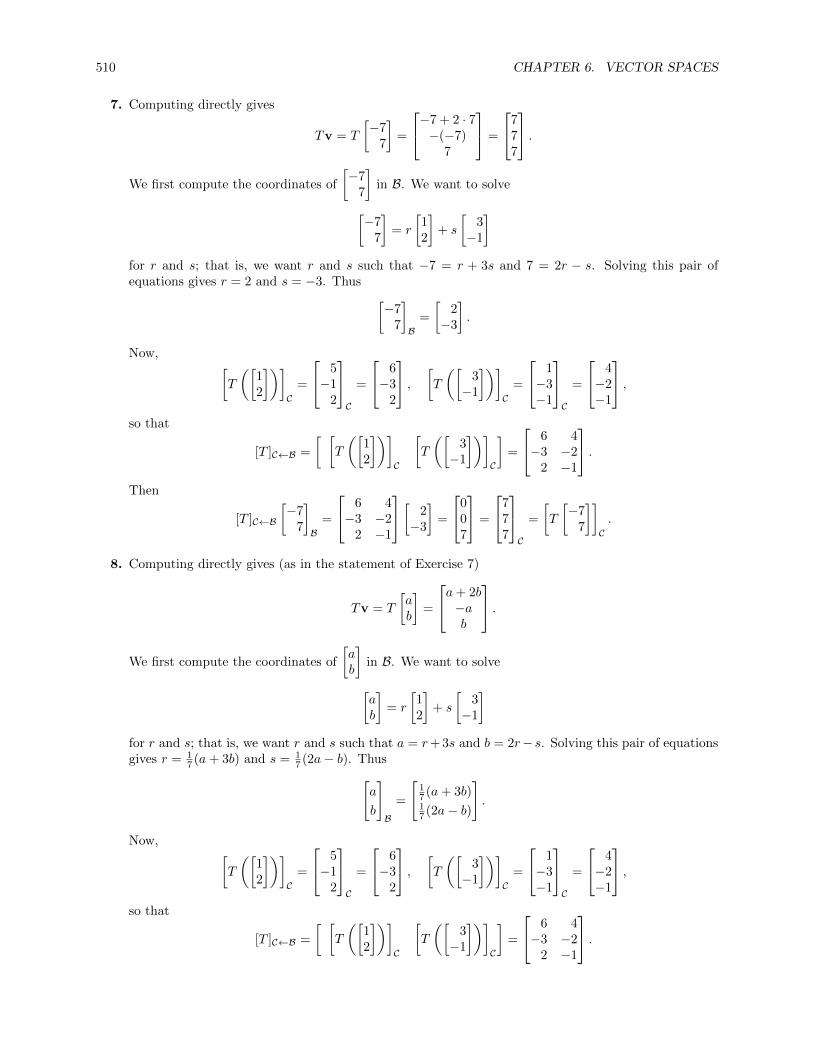
510 CHAPTER 6. VECTOR SPACES
7. Computing directly gives
Tv = T
[−7
7
]=
−7 + 2 · 7−(−7)
7
=
777
.We first compute the coordinates of
[−7
7
]in B. We want to solve
[−7
7
]= r
[12
]+ s
[3−1
]for r and s; that is, we want r and s such that −7 = r + 3s and 7 = 2r − s. Solving this pair ofequations gives r = 2 and s = −3. Thus [
−77
]B
=
[2−3
].
Now, [T
([12
])]C
=
5−1
2
C
=
6−3
2
, [T
([3−1
])]C
=
1−3−1
C
=
4−2−1
,so that
[T ]C←B =
[ [T
([12
])]C
[T
([3−1
])]C
]=
6 4−3 −2
2 −1
.Then
[T ]C←B
[−7
7
]B
=
6 4−3 −2
2 −1
[ 2−3
]=
007
=
777
C
=
[T
[−7
7
]]C.
8. Computing directly gives (as in the statement of Exercise 7)
Tv = T
[ab
]=
a+ 2b−ab
.We first compute the coordinates of
[ab
]in B. We want to solve
[ab
]= r
[12
]+ s
[3−1
]for r and s; that is, we want r and s such that a = r+ 3s and b = 2r− s. Solving this pair of equationsgives r = 1
7 (a+ 3b) and s = 17 (2a− b). Thus[
a
b
]B
=
[17 (a+ 3b)17 (2a− b)
].
Now, [T
([12
])]C
=
5−1
2
C
=
6−3
2
, [T
([3−1
])]C
=
1−3−1
C
=
4−2−1
,so that
[T ]C←B =
[ [T
([12
])]C
[T
([3−1
])]C
]=
6 4−3 −2
2 −1
.

6.6. THE MATRIX OF A LINEAR TRANSFORMATION 511
Then
[T ]C←B
[a
b
]B
=
6 4
−3 −2
2 −1
[ 17 (a+ 3b)17 (2a− b)
]
=
67 (a+ 3b) + 4
7 (2a− b)− 3
7 (a+ 3b)− 27 (2a− b)
27 (a+ 3b)− 1
7 (2a− b)
=
2a+ 2b
−a− bb
=
a+ 2b
−ab
C
=
[T
[a
b
]]C
.
9. Computing directly gives
Tv = TA = AT =
[a cb d
].
Since A = aE11 + bE12 + cE21 + dE22, the coordinate vector of A in B is
[A]B =
abcd
.Now,
[TE11]C = [ET11]C = [E11]C =
1000
C
=
1000
,
[TE12]C = [ET12]C = [E21]C =
[0 01 0
]C
=
0010
,
[TE21]C = [ET21]C = [E12]C =
[0 10 0
]C
=
0100
,
[TE22]C = [ET22]C = [E22]C =
[0 00 1
]C
=
0001
.Therefore
[T ]C←B =[
[TE11]C [TE12]C [TE21]C [TE22]C]
=
1 0 0 00 0 1 00 1 0 00 0 0 1
.Then
[T ]C←B[A]B =
1 0 0 00 0 1 00 1 0 00 0 0 1
abcd
=
acbd
=
[a cb d
]C
= [TA]C .

512 CHAPTER 6. VECTOR SPACES
10. Computing directly gives
Tv = TA = AT =
[a cb d
].
Since A = aE11 + bE12 + cE21 + dE22, the coordinate vector of A in B is
[A]B =
dcba
.Now,
[TE22]C = [ET22]C = [E22]C =
[0 00 1
]C
=
0010
,
[TE21]C = [ET21]C = [E12]C =
[0 10 0
]C
=
1000
,
[TE12]C = [ET12]C = [E21]C =
[0 01 0
]C
=
0100
,
[TE11]C = [ET11]C = [E11]C =
1000
C
=
0001
.Therefore
[T ]C←B =[
[TE22]C [TE21]C [TE12]C [TE11]C]
=
0 1 0 00 0 1 01 0 0 00 0 0 1
.Then
[T ]C←B[A]B =
0 1 0 00 0 1 01 0 0 00 0 0 1
dcba
=
cbda
=
[a cb d
]C
= [TA]C .
11. Computing directly gives
Tv = TA =
[a bc d
] [1 −1−1 1
]−[
1 −1−1 1
] [a bc d
]=
[a− b b− ac− d d− c
]−[a− c b− dc− a d− b
]=
[c− b d− aa− d b− c
].
Since A = aE11 + bE12 + cE21 + dE22, the coordinate vector of A in B is
[A]B =
abcd
.

6.6. THE MATRIX OF A LINEAR TRANSFORMATION 513
Now,
[TE11]C = [E11B −BE11]C =
[0 −11 0
]C
=
0−1
10
,
[TE12]C = [E12B −BE12]C =
[−1 0
0 1
]C
=
−1
001
,
[TE21]C = [E21B −BE21]C =
[1 00 −1
]C
=
100−1
,
[TE22]C = [E22B −BE22]C =
[0 1−1 0
]C
=
01−1
0
.Therefore
[T ]C←B =[
[TE11]C [TE12]C [TE21]C [TE22]C]
=
0 −1 1 0−1 0 0 1
1 0 0 −10 1 −1 0
.Then
[T ]C←B[A]B =
0 −1 1 0−1 0 0 1
1 0 0 −10 1 −1 0
abcd
=
c− bd− aa− db− c
=
[c− b d− aa− d b− c
]C
= [TA]C .
12. Computing directly gives
Tv = TA =
[a bc d
]−[a cb d
]=
[0 b− c
c− b 0
].
Using the given basis B for M22, the coordinate vector of A is
[A]B =
abcd
.Now,
[TE11]C = [E11 − ET11]C =
0000
, [TE12]C = [E12 − ET12]C = [E12 − E21]C =
01−1
0
,
[TE21]C = [E21 − ET21]C = [E21 − E12]C =
0−1
10
, [TE22]C = [E22 − ET22]C =
0000
.

514 CHAPTER 6. VECTOR SPACES
Therefore
[T ]C←B =[
[TE22]C [TE21]C [TE12]C [TE11]C]
=
0 0 0 00 1 −1 00 −1 1 00 0 0 0
.Then
[T ]C←B[A]B =
0 0 0 00 1 −1 00 −1 1 00 0 0 0
abcd
=
0
b− cc− b
0
=
[0 b− c
c− b 0
]C
= [TA]C .
13. (a) If a sinx+ b cosx ∈W , then
D(a sinx+ b cosx) = D(a sinx) +D(b cosx) = aD sinx+ bD cosx = a cosx− b sinx ∈W.
(b) Since
[sinx]B =
[10
], [cosx]B =
[01
],
then
[D sinx]B = [cosx]B =
[01
], [D cosx]B = [− sinx]B =
[−1
0
], ⇒ [D]B =
[0 −11 0
].
(c) [f(x)]B = [3 sinx− 5 cosx]B =
[3−5
], so
[D(f(x))]B = [D]B[f(x)]B =
[0 −11 0
] [3−5
]=
[53
],
so that D(f(x)) = f ′(x) = 5 sinx+ 3 cosx. Directly, since (sinx)′ = cosx and (cosx)′ = − sinx,we also get f ′(x) = 3 cosx− 5(− sinx) = 5 sinx+ 3 cosx.
14. (a) If ae2x + be−2x ∈W , then
D(ae2x + be−2x) = D(ae2x) +D(be−2x) = aDe2x + bDe−2x = (2a)e2x + (−2b)e−2x ∈W.
(b) Since
[e2x]B =
[10
], [e−2x]B =
[01
],
then
[De2x]B = [2e2x]B =
[20
], [De−2x]B = [−2e−2x]B =
[0−2
], ⇒ [D]B =
[2 00 −2
].
(c) [f(x)]B = [e2x − 3e−2x]B =
[1−3
], so
[D(f(x))]B = [D]B[f(x)]B =
[2 00 −2
] [1−3
]=
[26
],
so that D(f(x)) = f ′(x) = 2e2x + 6e−3x. Directly, f ′(x) = e2x · 2− 3e−2x · (−2) = 2e2x + 6e−3x.
15. (a) Since
[e2x]B =
100
, [e2x cosx]B =
010
, [e2x sinx]B =
001
,

6.6. THE MATRIX OF A LINEAR TRANSFORMATION 515
then
[De2x]B = [2e2x]B =
200
,[D(e2x cosx)]B = [2e2x cosx− e2x sinx]B =
02−1
,[D(e2x sinx)]B = [2e2x sinx+ e2x cosx]B =
012
.Thus
[D]B =
2 0 00 2 10 −1 2
.
(b) [f(x)]B = [3e2x − e2x cosx+ 2e2x sinx]B =
3−1
2
, so
[D(f(x))]B = [D]B[f(x)]B =
2 0 00 2 10 −1 2
3−1
2
=
605
,so that D(f(x)) = f ′(x) = 6e2x + 5e2x sinx. Directly,
f ′(x) = 3e2x · 2− (2e2x cosx− e2x sinx) + (4e2x sinx+ 2e2x cosx) = 6e2x + 5e2x sinx.
16. (a) Since
[cosx]B =
1000
, [sinx]B =
0100
, [x cosx]B =
0010
, [x sinx]B =
0001
,then
[D cosx]B = [− sinx]B =
0−1
00
, [D sinx]B = [cosx]B =
1000
,
[D(x cosx)]B = [cosx− x sinx]B =
100−1
, [D(x sinx)]B = [sinx+ x cosx]B =
0110
.Thus
[D]B =
0 1 1 0−1 0 0 1
0 0 0 10 0 −1 0
.

516 CHAPTER 6. VECTOR SPACES
(b) [f(x)]B = [cosx+ 2x cosx]B =
1020
, so
[D(f(x))]B = [D]B[f(x)]B =
0 1 1 0−1 0 0 1
0 0 0 10 0 −1 0
1020
=
2−1
0−2
,so that D(f(x)) = f ′(x) = 2 cosx− sinx− 2x sinx. Directly,
f ′(x) = − sinx+ 2 cosx− 2x sinx = 2 cosx− sinx− 2x sinx.
17. (a) Let p(x) = a+ bx; then
(S ◦ T )p(x) = S(Tp(x)) = S
([p(0)p(1)
])= S
[a
a+ b
]=
[a− 2(a+ b)2a− (a+ b)
]=
[−a− 2ba− b
].
Then
[(S ◦ T )(1)]D =
[−1
1
]D
=
[−1
1
], [(S ◦ T )(x)]D =
[−2−1
]D
=
[−2−1
],
so that
[S ◦ T ]D←B =
[−1 −2
1 −1
].
(b) We have
[T (1)]C =
[11
]C
=
[11
], [T (x)]C =
[01
]C
=
[01
],
so that
[T ]C←B =
[1 01 1
].
Next, [S
[10
]]D
=
[12
]D
=
[12
],
[S
[01
]]D
=
[−2−1
]D
=
[−2−1
],
so that
[S]D←C =
[1 −22 −1
].
Then
[S ◦ T ]D←B = [S]D←C [T ]C←B =
[1 −22 −1
] [1 01 1
]=
[−1 −2
1 −1
],
which matches the result from part (a).
18. (a) Let p(x) = a+ bx; then
(S ◦ T )p(x) = S(Tp(x)) = S(a+ b(x+ 1)) = S((a+ b) + bx) = (a+ b) + b(x+ 1) = (a+ 2b) + bx.
Then
[(S ◦ T )(1)]D =
100
D
=
100
, [(S ◦ T )(x)]D =
210
D
=
210
,so that
[S ◦ T ]D←B =
1 20 10 0
.

6.6. THE MATRIX OF A LINEAR TRANSFORMATION 517
(b) We have
[T (1)]C = [1]C =
100
C
=
100
, [T (x)]C = [x+ 1]C =
110
C
=
110
,so that
[T ]C←B =
1 10 10 0
.Next,
[S(1)]D = [1]D =
100
, [S(x)]D = [x+ 1]D =
110
,[S(x2)]D = [(x+ 1)2]D = [x2 + 2x+ 1]D =
121
,so that
[S]D←C =
1 1 10 1 20 0 1
.Then
[S ◦ T ]D←B = [S]D←C [T ]C←B =
1 1 10 1 20 0 1
1 10 10 0
=
1 20 10 0
,which matches the result from part (a).
19. In Exercise 1, the basis for P1 in both the domain and codomain was already the standard basis E ,so we can use the matrix computed there:
[T ]E←E =
[0 1−1 0
].
Since this matrix has determinant 1, it is invertible, so that T is invertible as well. Then
[T−1(a+ bx)]E←E = ([T ]E←E)−1
[ab
]=
[0 1−1 0
]−1 [ab
]=
[0 −11 0
] [ab
]=
[−ba
].
So T−1(a+ bx) = −b+ ax.
20. From Exercise 5,
[T ]C←B =
[1 0 01 1 1
].
Since this matrix is not square, it is not invertible, so that T is not invertible.
21. We first compute [T ]E←E , where E = {1, x, x2} is the standard basis:
[T (1)]E = [1]E =
100
, [T (x)]E = [x+ 2]E =
210
, [T (x2)]E = [(x+ 2)2]E = [x2 + 4x+ 4]E =
441
,so that
[T ]E←E =
1 2 40 1 40 0 1
.

518 CHAPTER 6. VECTOR SPACES
Since this is an upper triangular matrix with nonzero diagonal entries, it is invertible, so that T isinvertible as well. To find T−1, we have
[T−1(a+ bx+ cx2)]E←E = ([T ]E←E)−1
abc
=
1 2 40 1 40 0 1
−1 abc
=
1 −2 40 1 −40 0 1
abc
=
a− 2b+ 4cb− 4cc
.So T−1(a+ bx) = (a− 2b+ 4c) + (b− 4c)x+ cx2 = a+ b(x− 2) + c(x− 2)2 = p(x− 2).
22. We first compute [T ]E←E , where E = {1, x, x2} is the standard basis:
[T (1)]E = [0]E =
000
, [T (x)]E = [1]E =
100
, [T (x2)]E = [2x]E =
020
,so that
[T ]E←E =
0 1 00 0 20 0 0
.Since this is an upper triangular matrix with a zero entry on the diagonal, it has determinant zero, sois not invertible; therefore, T is not invertible either.
23. We first compute [T ]E←E , where E = {1, x, x2} is the standard basis:
[T (1)]E = [1 + 0]E = [1]E =
100
, [T (x)]E = [x+ 1]E =
110
, [T (x2)]E = [x2 + 2x]E =
021
,so that
[T ]E←E =
1 1 00 1 20 0 1
.Since this is an upper triangular matrix with nonzero diagonal entries, it is invertible, so that T isinvertible as well. To find T−1, we have
[T−1(a+ bx+ cx2)]E←E = ([T ]E←E)−1
abc
=
1 1 00 1 20 0 1
−1 abc
=
1 −1 20 1 −20 0 1
abc
=
a− b+ 2cb− 2cc
.So T−1(a+ bx+ cx2) = (a− b+ 2c) + (b− 2c)x+ cx2.

6.6. THE MATRIX OF A LINEAR TRANSFORMATION 519
24. We first compute [T ]E←E , where E = {E11, E12, E21, E22} is the standard basis:
[TE11]E =
([1 00 0
] [3 22 1
])E
=
[3 20 0
]E
=
3200
,
[TE12]E =
([0 10 0
] [3 22 1
])E
=
[2 10 0
]E
=
2100
,
[TE21]E =
([0 01 0
] [3 22 1
])E
=
[0 03 2
]E
=
0032
,
[TE22]E =
([0 00 1
] [3 22 1
])E
=
[0 02 1
]E
=
0021
,so that
[T ]E←E =
3 2 0 02 1 0 00 0 3 20 0 2 1
.This matrix is block triangular, and each diagonal block is invertible, so it is invertible and thereforeT is invertible as well. To find T−1, we have
[T−1
[a bc d
]]E←E
= ([T ]E←E)−1
abcd
=
3 2 0 02 1 0 00 0 3 20 0 2 1
−1
abcd
=
−1 2 0 0
2 −3 0 00 0 −1 20 0 2 −3
abcd
=
−a+ 2b2a− 3b−c+ 2d2c− 3d
.So T−1
[a bc d
]=
[−a+ 2b 2a− 3b−c+ 2d 2c− 3d
].
25. From Exercise 11, since the bases given there were both the standard basis,
[T ]E←E =
0 −1 1 0−1 0 0 1
1 0 0 −10 1 −1 0
.This matrix has determinant zero (for example, the second and third rows are multiples of one another),so that T is not invertible.
26. From Exercise 12, since the bases given there were both the standard basis,
[T ]E←E =
0 0 0 00 1 −1 00 −1 1 00 0 0 0
.This matrix has determinant zero, so that T is not invertible.

520 CHAPTER 6. VECTOR SPACES
27. In Exercise 13, the basis is B = {sinx, cosx}. Using the method of Example 6.83,[∫(a sinx+ b cosx) dx
]B
= [D]−1B←B
[ab
].
Using [D]B←B from Exercise 13, we get[∫(sinx− 3 cosx) dx
]B
=
[0 −11 0
]−1 [1−3
]=
[0 1−1 0
] [1−3
]=
[−3−1
].
So∫
(sinx− 3 cosx) dx = −3 sinx− cosx+ C. This is the same answer as integrating directly.
28. In Exercise 14, the basis is B = {e2x, e−2x}. Using the method of Example 6.83,[∫ (ae2x + be−2x
)dx
]B
= [D]−1B←B
[ab
].
Using [D]B←B from Exercise 14, we get[∫5e−2x dx
]B
=
[2 0
0 −2
]−1 [0
5
]=
[12 0
0 − 12
][0
5
]=
[0
− 52
].
So∫
5e−2x dx = − 52e−2x + C. This is the same answer as integrating directly.
29. In Exercise 15, the basis is B = {e2x, e2x cosx, e2x sinx}. Using the method of Example 6.83,[∫ (ae2x + be−2x
)dx
]B
= [D]−1B←B
[ab
].
Using [D]B←B from Exercise 15, we get
[∫ (e2x cosx− 2e2x sinx
)dx
]B
=
2 0 0
0 2 1
0 −1 2
−1 0
1
−2
=
12 0 0
0 25 − 1
5
0 15
25
0
1
−2
=
045
− 35
.So∫ (e2x cosx− 2e2x sinx
)dx = 4
5e2x cosx− 3
5e2x sinx+ C. Checking via differentiation gives(
4
5e2x cosx− 3
5e2x sinx+ C
)′=
4
5
(2e2x cosx− e2x sinx
)− 3
5
(2e2x sinx+ e2x cosx
)= e2x cosx− 2e2x sinx.
30. In Exercise 16, the basis is B = {cosx, sinx, x cosx, x sinx}. Using the method of Example 6.83,
[∫(a cosx+ b sinx+ cx cosx+ dx sinx) dx
]B
= [D]−1B←B
abcd
.Using [D]B←B from Exercise 16, we get
[∫(x cosx+ x sinx) dx
]B
=
0 1 1 0−1 0 0 1
0 0 0 10 0 −1 0
−1
0011
=
0 −1 1 01 0 0 10 0 0 −10 0 1 0
0011
=
11−1
1
So∫
(x cosx+ x sinx) dx = cosx+ sinx− x cosx+ x sinx+ C. Checking via differentiation gives
(cosx+ sinx− x cosx+ x sinx+ C)′
= − sinx+ cosx− cosx+ x sinx+ sinx+ x cosx
= x cosx+ x sinx.

6.6. THE MATRIX OF A LINEAR TRANSFORMATION 521
31. With E = {e1, e2}, we have
[Te1]E =
[−4 · 0
1 + 5 · 0
]E
=
[01
]E
=
[01
], [Te2]E =
[−4 · 1
0 + 5 · 1
]E
=
[−4
5
]E
=
[−4
5
].
Therefore
[T ]E =
[0 −41 5
].
Using the method of Example 6.86(b), the eigenvectors of [T ]E will give us a diagonalizing basis C.Using methods from Chapter 4, we find the eigenvalues and corresponding eigenvectors to be
λ1 = 4, v1 =
[−1
1
], λ2 = 1, v2 =
[−4
1
].
Thus
C =
{[−1
1
],
[−4
1
]}, and [T ]C =
[−1 −4
1 1
]−1
[T ]E
[−1 −4
1 1
]=
[4 00 1
]32. With E = {e1, e2}, we have
[Te1]E =
[1− 01 + 0
]E
=
[11
]E
=
[11
], [Te2]E =
[0− 10 + 1
]E
=
[−1
1
]E
=
[−1
1
].
Therefore
[T ]E =
[1 −11 1
].
Using the method of Example 6.86(b), the eigenvectors of [T ]E will give us a diagonalizing basis C.Using methods from Chapter 4, we find the eigenvalues and corresponding eigenvectors to be
λ1 = 1 + i, v1 =
[i1
], λ2 = 1− i, v2 =
[−i
1
].
Since the eigenvectors are not real, T is not diagonalizable.
33. With E = {1, x}, we have
[T (1)]E = [4 + x]E =
[41
]E
=
[41
], [T (x)]E = [2 + 3x]E =
[23
]E
=
[23
].
Therefore
[T ]E =
[4 21 3
].
Using the method of Example 6.86(b), the eigenvectors of [T ]E will give us a diagonalizing basis C.Using methods from Chapter 4, we find the eigenvalues and corresponding eigenvectors to be
λ1 = 5, v1 =
[21
], λ2 = 2, v2 =
[−1
1
].
Thus
C =
{[21
],
[−1
1
]}, and [T ]C =
[2 −11 1
]−1
[T ]E
[2 −11 1
]=
[5 00 2
].
34. With E = {1, x, x2}, we have
[T (1)]E = [1]E =
100
E
=
100
, [T (x)]E = [x+ 1]E =
110
E
=
110
,[T (x2)]E = [(x+ 1)2]E = [x2 + 2x+ 1]E =
121
E
=
121
.

522 CHAPTER 6. VECTOR SPACES
Therefore
[T ]E =
1 1 10 1 20 0 1
.Using the method of Example 6.86(b), the eigenvectors of [T ]E will give us a diagonalizing basis C. Sincethis is an upper triangular matrix with 1s on the diagonal, the only eigenvalue is 1; using methods from
Chapter 4 we find the eigenspace to be one-dimensional with basis
100
. Thus T is not diagonalizable.
35. With E = {1, x}, we have
[T (1)]E = [1 + x · 0]E = [1]E =
[10
]E
=
[10
], [T (x)]E = [x+ x · 1]E = [2x]E =
[02
]E
=
[02
].
Therefore
[T ]E =
[1 00 2
].
Thus T is already diagonal with respect to the standard basis E .
36. With E = {1, x, x2}, we have
[T (1)]E = [1]E =
100
E
=
100
,[T (x)]E = [3x+ 2]E =
230
E
=
230
,[T (x2)]E = [(3x+ 2)2]E = [9x2 + 12x+ 4]E =
4129
E
=
9124
.Therefore
[T ]E =
1 2 40 3 120 0 9
.Using the method of Example 6.86(b), the eigenvectors of [T ]E will give us a diagonalizing basis C.Since this is an upper triangular matrix with 1s on the diagonal, the eigenvalues are 1, 3, and 4; usingmethods from Chapter 4 we find the corresponding eigenvectors to be
λ1 = 1, v1 =
100
, λ2 = 3, v2 =
110
, λ3 = 9, v3 =
121
.Thus
C =
1
00
,1
10
,1
21
, and [T ]C =
1 1 10 1 20 0 1
−1
[T ]E
1 1 10 1 20 0 1
=
1 0 00 3 00 0 9
.
37. Let ` have direction vector d =
[d1
d2
], and let T be the reflection in `. Let d′ =
[−d2
d1
]. As in Example
6.85, we may as well assume for simplicity that d is a unit vector; then d′ is as well. Continuing

6.6. THE MATRIX OF A LINEAR TRANSFORMATION 523
to follow Example 6.85, D = {d,d′} is a basis for R2. Since d′ is orthogonal to d, it follows thatTd′ = −d′. Thus
[T (d)]D = [d]D =
[10
], [T (d′)]D = [−d′]D =
[0−1
].
Thus
[T ]D =
[1 00 −1
].
Now, [T ]E = PE←D[T ]DPD←E , so we must find PE←D. The columns of this matrix are the expressionof the basis vectors of D in the standard basis E , so we have
PE←D =
[d1 d2
d2 −d1
].
Since we assumed d was a unit vector, this is an orthogonal matrix, so that
[T ]E = PE←D[T ]DPD←E = PE←D[T ]DP−1E←D = PE←D[T ]DP
TE←D
=
[d1 d2
d2 −d1
] [1 00 −1
] [d1 d2
d2 −d1
]=
[d2
1 − d22 2d1d2
2d1d2 d22 − d2
1
].
Note that this is the same as the answer from Exercise 26 in Section 3.6, with the assumption that dis a unit vector.
38. Let T be the projection onto W . From Example 5.11, we have an orthogonal basis for R2,u1 =
110
, u2 =
−111
, u3 =
1−1
2
,
where {u1,u2} is a basis for W and {u3} is a basis for W⊥. Then
[T (u1)]D =
100
, [T (u2)]D =
010
, [T (u3)]D =
000
, so that [T ]D =
1 0 00 1 00 0 0
.Further, since the columns of PE←D are the expression of the basis vectors of D in the standard basisE ,
PE←D =
1 −1 1
1 1 −1
0 1 2
⇒ P−1E←D =
12
12 0
− 13
13
13
16 − 1
613
.Thus
[T ]E = PE←D[T ]DPD←E = PE←D[T ]DP−1E←D
=
1 −1 1
1 1 −1
0 1 2
1 0 0
0 1 0
0 0 0
12
12 0
− 13
13
13
16 − 1
613
=
56
16 − 1
316
56
13
− 13
13
13
.
If v =
3−1
2
, then
projW v = [T ]E [v]E =
56
16 − 1
316
56
13
− 13
13
13
3
−1
2
=
5313
− 23
,which is the same as was found in Example 11 in Section 5.2.

524 CHAPTER 6. VECTOR SPACES
39. Let B = {v1, . . . ,vn}, and suppose that A is such that A[v]B = [Tv]C for all v ∈ V . Then A[vi]B =[Tvi]C . But [vi]B = ei since the vi are the basis vectors of B, so this equation says that Aei = [Tvi]C .The left-hand side of this equation is the ith column of A, while the right-hand side is the ith columnof [T ]C←B. Thus those ith columns are equal; since this holds for all i, we get A = [T ]C←B.
40. Suppose that [v]B ∈ null([T ]C←B). That means that
0 = [T ]C←B[v]B = [Tv]C ,
so that [Tv]C = 0 and thus v ∈ ker(T ). Similarly, if v ∈ ker(T ), then
0 = [Tv]C = [T ]C←B[v]B,
so that [v]B ∈ null([T ]C←B). Then the map V → Rn : v 7→ [v]B is an isomorphism mapping ker(T ) tonull([T ]C←B), so the two subspaces are isomorphic and thus have the same dimension. So nullity(T ) =nullity([T ]C←B).
41. Suppose B = {b1, . . . ,bn}. Then[T ]C←B[bi]B = [T (bi)]C
by definition of the matrix of T with respect to these bases, and denote by ai the columns of [T ]C←B.Then rank([T ]C←B) = dim col[T ]C←B, which is the number of linearly independent ai, and rank(T ) =dim range(T ), which is the number of linearly independent T (vi). Now, since
ai = [T ]C←B[bi]B = [T (bi)]C
we see that {ai1 ,ai2 , . . . ,aim} are linearly independent if and only if {T (bi1), . . . , T (b)im} are linearlyindependent, so col(A) = span(ai1 ,ai2 , . . . ,aim) if and only if range(T ) = span(T (bi1), . . . , T (b)im)and therefore rank(A) = rank(T ).
42. T is diagonalizable if and only if there is some basis C and matrix P such that [T ]C = P−1AP isdiagonal. Thus if T is diagonalizable, so is A. For the reverse, if A is diagonalizable, then the basis Cwhose elements are the columns of P is a basis in which [T ]C is diagonal.
43. Let dimV = n and dimW = m. Then [T ]C←B is an m × n matrix, and by Theorem 3.26 in Section3.5, rank([T ]C←B) + nullity([T ]C←B) = n. But by Exercises 40 and 41, rank([T ]C←B) = rank(T ) andnullity([T ]C←B) = nullity(T ); since dimV = n, we get
dimV = rank(T ) + nullity(T ).
44. Claim that [T ]C′←B′ = PC′←C [T ]C←BPB←B′ . To prove this, it is enough to show that for all x ∈ V ,
[x]C′ = PC′←C [T ]C←BPB←B′ [x]B′
since the matrix of T with respect to B′ and C′ is unique by Exercise 39. And indeed
PC′←C [T ]C←BPB←B′ [x]B′ = PC′←C [T ]C←B (PB←B′ [x]B′) = PC′←C ([T ]C←B[x]B) = PC′←C [x]C = [x]C′ .
45. For T ∈ L(V,W ), define ϕ(T ) = [T ]C←B ∈Mmn. Claim that ϕ is an isomorphism. We must first showit is linear:
ϕ(S + T ) = [(S + T )]C←B
=[
[(S + T )b1]C · · · [(S + T )bn]C]
=[
[Sb1]C + [Tb1]C · · · [Sbn]C + [Tbn]C]
=[
[Sb1]C · · · [Sbn]C]
+[
[Tb1]C · · · [Tbn]C]
= ϕ(S) + ϕ(T ).

Exploration: Tiles, Lattices, and the Crystallographic Restriction 525
Similarly
ϕ(cS) = [(cS)]C←B
=[
[(cS)b1]C · · · [(cS)bn]C]
=[c[Sb1]C · · · c[Sbn]C
]= c
[[Sb1]C · · · [Sbn]C
]= cϕ(S).
Next we show that kerϕ = 0, so that ϕ is one-to-one. Suppose that ϕ(T ) = 0. That means that[T ]C←B = [0]mn, so that nullity([T ]C←B) = n. By Exercise 40, this is equal to nullity(T ). Thusnullity(T ) = n = dimV , so that T is the zero linear transformation, showing that ϕ is one-to-one.
Finally, since dimMmn = mn, we will have shown that ϕ is an isomorphism if we prove thatdimL(V,W ) = mn. But if {v1, . . . ,vn} and {w1, . . . ,wm} are bases for V and W , then a linearmap from V to W sends each vi to some linear combination of the wj , so it is a sum of maps that sendvi to wk and the other vi to zero. There are mn of these maps, which are clearly linearly independent,so that dimL(V,W ) = mn.
46. From Exercise 45 with W = R, we have dimW = dimR = 1, so that M1n∼= V . Thus
V ∗ = L(V,W ) = L(V,R) ∼= M1n∼= V.
Exploration: Tiles, Lattices, and the Crystallographic Restriction
1. Let P be the pattern in Figure 6.15. We are given, from the figure, that P+u = P and that P+v = P .Therefore if a is a positive integer, then P +au = (P +u) + (a− 1)u = P + (a− 1)u, and by inductionthis is just P . Similarly if b is a positive integer then P + bv = (P + v) + (b − 1)v = P + (b − 1)v,which again by induction is equal to P . If a is a negative integer, then since P + (−a)u = P , it followsthat P = P − (−a)u = P + au, and similarly for b < 0 and v.
2. The lattice points correspond to centersof the trefoils in Figure 6.15.
u
v
-3 -2 -1 1 2 3
-1.5
-1.
-0.5
0.5
1.
1.5
3. Let θ be the smallest positive angle through which the lattice exhibits rotational symmetry. Let RθOdenote the operation of rotation through an angle θ > 0 around a center of rotation O, and let P be apattern or lattice. Now we have
RnθO (P ) =(RθO)n
(P ) = P, n ∈ Z, n > 0,
since rotation through nθ is the same as applying a rotation through θ n times. If n < 0, then rotatingthrough nθ gives a figure which, if rotated back through (−n)θ, is P , so it must be P as well. Thisshows that P is rotationally symmetric under any integer multiple of θ.
Next, let m be the smallest positive integer such that mθ ≥ 360◦, and suppose that mθ = 360◦ + ϕ.
Note that R360◦
O (P ) = P , so that R360◦+ϕO (P ) = RϕO(P ). We want to show that 360◦
θ is an integer, soit suffices to show that ϕ = 0. Now, since m is minimal, we know that
mθ − ϕ = 360◦ > (m− 1)θ,
so that mθ − ϕ > mθ − θ and thus −ϕ > −θ, so that ϕ < θ. But
P = RmθO (P ) = R360◦+ϕO (P ) = RϕO(P ),
and we see that the lattice is rotationally symmetric under a rotation of ψ < θ′. Since ϕ ≥ 0 and θ isthe smallest positive such angle, it follows that ϕ = 0. Thus θ = 360◦
m .
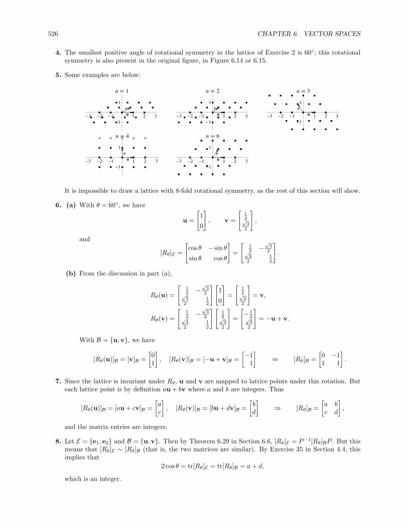
526 CHAPTER 6. VECTOR SPACES
4. The smallest positive angle of rotational symmetry in the lattice of Exercise 2 is 60◦; this rotationalsymmetry is also present in the original figure, in Figure 6.14 or 6.15.
5. Some examples are below:
u
v
-3 -2 -1 1 2 3
-1
1
n � 1
u
v
-3 -2 -1 1 2 3
-1
1
n � 2
u
v
-3 -2 -1 1 2 3
-1
1
n � 3
u
v
-3 -2 -1 1 2 3
-1
1
n � 4
u
v
-3 -2 -1 1 2 3
-1
1
n � 6
It is impossible to draw a lattice with 8-fold rotational symmetry, as the rest of this section will show.
6. (a) With θ = 60◦, we have
u =
[1
0
], v =
[12√3
2
],
and
[Rθ]E =
[cos θ − sin θ
sin θ cos θ
]=
[12 −
√3
2√3
212
].
(b) From the discussion in part (a),
Rθ(u) =
[12 −
√3
2√3
212
][1
0
]=
[12√3
2
]= v,
Rθ(v) =
[12 −
√3
2√3
212
][12√3
2
]=
[− 1
2√3
2
]= −u + v.
With B = {u,v}, we have
[Rθ(u)]B = [v]B =
[01
], [Rθ(v)]B = [−u + v]B =
[−1
1
]⇒ [Rθ]B =
[0 −11 1
].
7. Since the lattice is invariant under Rθ, u and v are mapped to lattice points under this rotation. Buteach lattice point is by definition au + bv where a and b are integers. Thus
[Rθ(u)]B = [au + cv]B =
[ac
], [Rθ(v)]B = [bu + dv]B =
[bd
]⇒ [Rθ]B =
[a bc d
],
and the matrix entries are integers.
8. Let E = {e1, e2} and B = {u,v}. Then by Theorem 6.29 in Section 6.6, [Rθ]E = P−1[Rθ]BP . But thismeans that [Rθ]E ∼ [Rθ]B (that is, the two matrices are similar). By Exercise 35 in Section 4.4, thisimplies that
2 cos θ = tr[Rθ]E = tr[Rθ]B = a+ d,
which is an integer.

6.7. APPLICATIONS 527
9. If 2 cos θ = m is an integer, then m must be 0, ±1, or ±2, so the angles are angles whose cosines are0, ± 1
2 , or ±1; these angles are
θ = 60◦, 90◦, 120◦, 180◦, 240◦, 270◦, 300◦, 360◦,
corresponding to
n = 1, 2, 3, 4, or 6.
These are the only possible n-fold rotational symmetries.
10. Left to the reader.
6.7 Applications
1. Here a = −3, so by Theorem 6.32, {e3t} is a basis for solutions, which therefore have the formy(t) = ce3t. Since y(1) = ce3 = 2, we have c = 2e−3, so that y(t) = 2e−3e3t = 2e3t−3.
2. Here a = 1, so by Theorem 6.32, {e−t} is a basis for solutions, which therefore have the form x(t) = ce−t.Since x(1) = ce−1 = 1, we have c = e, so that x(t) = ee−t = e1−t.
3. y′′ − 7y′ + 12y = 0 corresponds to the characteristic equation λ2 − 7λ+ 12 = (λ− 3)(λ− 4) = 0. Thenλ1 = 3 and λ2 = 4, so Theorem 6.33 tells us that the general solution has the form y(t) = c1e
3t+ c2e4t.
Then
y(0) = 1
y(1) = 1⇒ c1 + c2 = 1
e3c1 + e4c2 = 1⇒
c1 =1− e4
e3 − e4
c2 =e3 − 1
e3 − e4
so that
y(t) =1
e3 − e4
((1− e4
)e3t +
(e3 − 1
)e4t).
4. x′′+x′−12x = 0 corresponds to the characteristic equation λ2+λ−12 = (λ−3)(λ+4) = 0. Then λ1 = 3and λ2 = −4, so Theorem 6.33 tells us that the general solution has the form x(t) = c1e
3t + c2e−4t.
Then
x(0) = 0
x′(0) = 1⇒ c1 + c2 = 0
3c1 − 4c2 = 1⇒
c1 =1
7
c2 = −1
7
so that
y(t) =1
7
(e3t − e−4t
).
5. f ′′ − f ′ − f = 0 corresponds to the characteristic equation λ2 − λ − 1 = 0, so that λ1 = 1+√
52 and
λ2 = 1−√
52 . Therefore by Theorem 6.33, the general solution is f(t) = c1e
(1+√
5)t/2 + c2e(1−√
5)t/2. So
f(0) = 0
f(1) = 1⇒
c1 + c2 = 0
e(1+√
5)/2c1 + e(1−√
5)/2c2 = 1⇒
c1 =e(√
5−1)/2
e√
5 − 1
c2 = −e(√
5−1)/2
e√
5 − 1
so that
f(t) =e(√
5−1)/2
e√
5 − 1
(e(1+
√5)t/2 − e(1−
√5)t/2
).

528 CHAPTER 6. VECTOR SPACES
6. g′′ − 2g = 0 corresponds to the characteristic equation λ2 − 2 = 0, so that λ1 =√
2 and λ2 = −√
2.
Therefore by Theorem 6.33, the general solution is g(t) = c1et√
2 + c2e−t√
2. So
g(0) = 1
g(1) = 0⇒
c1 + c2 = 1
e√
2c1 + e−√
2c2 = 0⇒
c1 = − 1
e2√
2 − 1
c2 =e2√
2
e2√
2 − 1
so that
g(t) =1
e2√
2 − 1
(−et√
2 + e2√
2−t√
2).
7. y′′ − 2y′ + y = 0 corresponds to the characteristic equation λ2 − 2λ + 1 = (λ − 1)2 = 0, so thatλ1 = λ2 = 1. Therefore by Theorem 6.33, the general solution is y(t) = c1e
t + c2tet. So
y(0) = 1
y(1) = 1⇒ c1 = 1
ec1 + ec2 = 1⇒
c1 = 1
c2 =1− ee
so that
y(t) = et +1− ee
tet = et + (1− e)tet−1.
8. x′′ + 4x′ + 4x = 0 corresponds to the characteristic equation λ2 + 4λ + 4 = (λ + 2)2 = 0, so thatλ1 = λ2 = −2. Therefore by Theorem 6.33, the general solution is x(t) = c1e
−2t + c2te−2t. So
x(0) = 1
x′(0) = 1⇒ c1 = 1
−2c1 + c2 = 1⇒
c1 = 1
c2 = 3
so thaty(t) = e−2t + 3te−2t.
9. y′′ − k2y = 0 corresponds to the characteristic equation λ2 − k2 = 0, so that λ1 = k and λ2 = −k.Therefore by Theorem 6.33, the general solution is y(t) = c1e
kt + c2e−kt. So
y(0) = 1
y′(0) = 1⇒ c1 + c2 = 1
kc1 − kc2 = 1⇒
c1 =k + 1
2k
c2 =k − 1
2k
so that
y(t) =1
2k
((k + 1)ekt + (k − 1)e−kt
).
10. y′′ − 2ky′ + k2y = 0 corresponds to the characteristic equation λ2 − 2kλ+ k2 = (λ− k)2 = 0, so thatλ1 = λ2 = k. Therefore by Theorem 6.33, the general solution is y(t) = c1e
kt + c2tekt. So
y(0) = 1
y(1) = 0⇒ c1 = 1
c1 + c2 = 0⇒
c1 = 1
c2 = −1
so thaty(t) = ekt − te−kt.
11. f ′′ − 2f ′ + 5f = 0 corresponds to the characteristic equation λ2 − 2λ+ 5 = 0, so that λ1 = 1 + 2i andλ2 = 1− 2i. Therefore by Theorem 6.33, the general solution is f(t) = c1e
t cos 2t+ c2et sin 2t. Then
f(0) = 1
f(π
4
)= 0
⇒ c1 = 1eπ/4c2 = 0
⇒c1 = 1
c2 = 0
so thaty(t) = et cos 2t.

6.7. APPLICATIONS 529
12. h′′ − 4h′ + 5h = 0 corresponds to the characteristic equation λ2 − 4λ+ 5 = 0, so that λ1 = 2 + i andλ2 = 2 − i. Therefore by Theorem 6.33, the general solution is h(t) = c1e
2t cos t + c2e2t sin t. Then
h′(t) = c1(2e2t cos t− e2t sin t) + c2(2e2t sin t+ e2t cos t), and
h(0) = 0
h′(0) = −1⇒ c1 = 0
2c1 + c2 = −1⇒
c1 = 0
c2 = −1
so thaty(t) = −e2t sin t.
13. (a) We start with p(t) = cekt; then p(0) = ce0k = c = 100, so that c = 100. Next, p(3) = 100e3k =1600, so that e3k = 16 and k = ln 16
3 . Hence
p(t) = 100e(ln 16/3)t = 100(eln 16
)t/3= 100 · 16t/3.
(b) The population doubles when p(t) = 100e(ln 16/3)t = 200. Simplifying gives
ln 16
3t = ln 2, so that t =
3 ln 2
ln 16=
3 ln 2
4 ln 2=
3
4.
The population doubles in 34 of an hour, or 45 minutes.
(c) We want to find t such that p(t) = 100e(ln 16/3)t = 1000000. Simplifying gives
ln 16
3t = ln 10000, so that t =
3 ln 10000
ln 16=
12 ln 10
4 ln 2=
3 ln 10
ln 2≈ 9.966 hours.
14. (a) Start with p(t) = cekt; then p(0) = ce0k = c = 76. Next, p(1) = 76e1k = 92, so that k = ln 9276 ,
and therefore p(t) = 76et ln(92/76). For the year 2000, we get
p(10) = 76e10 ln(92/76) ≈ 513.5.
This is almost twice the actual population in 2000.
(b) Start with p(t) = cekt; then p(0) = ce0k = c = 203. Next, p(1) = 203e1k = 227, so that k = ln 227203 ,
and therefore p(t) = 203et ln(227/203). For the year 2000, we get
p(3) = 203e3 ln(227/203) ≈ 283.8.
This is a pretty good approximation.
(c) Since the first estimate is very high but the second estimate is close, we can conclude that popula-tion growth was lower than exponential in the early 20th century, but has been close to exponentialsince 1970. This could be attributed for example to three major wars during the period from 1900to 1970.
15. (a) Let m(t) = ae−ct. Then m(0) = ae−c·0 = a = 50, so that m(t) = 50e−ct. Since the half-life is1590 years, we know that 25 mg will remain after that time, so that
m(1590) = 50e−1590c = 25.
Simplifying gives −1590c = ln 12 = − ln 2, so that c = ln 2
1590 . So finally, m(t) = 50e−t ln 2/1590.After 1000 years, the amount remaining is
m(1000) = 50e−1000 ln 2/1590 ≈ 32.33 mg.
(b) Only 10 mg will remain when m(t) = 10. Solving 50e−t ln 2/1590 = 10 gives
−t ln 2
1590= ln
1
5= − ln 5, so that t =
1590 ln 5
ln 2≈ 3692 years.

530 CHAPTER 6. VECTOR SPACES
16. With m(t) = ae−ct, a half-life of 5730 years means that m(5730) = ae−5730c = a2 , so that e−5730c = 1
2
and thus c = − ln(1/2)5730 = ln 2
5730 . To find out how old the posts are, we want to find t such that
m(t) = ae−t ln 2/5730 = 0.45a, which gives t = −5730 ln 0.45
ln 2≈ 6600 years.
17. Following Example 6.92, the general equation of the spring motion is x(t) = c1 cos√K t+ c2 sin
√K t.
Then x(0) = 10 = c1 cos 0 + c2 sin 0 = c1, so that c1 = 10. Then
x(10) = 5 = 10 cos 10√K + c2 sin 10
√K , so that c2 =
5− 10 cos 10√K
sin 10√K
.
Therefore the equation of the spring, giving its length at time t, is
c2 = 10 cos√K t+
5− 10 cos 10√K
sin 10√K
sin√K t.
18. From the analysis in Example 6.92, since K = km and m = 50, we have K = k
50 , so that
x(t) = c1 cos√K t+ c2 sin
√K t = c1 cos
√k
50t+ c2 sin
√k
50t.
Since the period of sin bt and cos bt are each 2πb , the fact that the period is 10 means that 2π√
k/50= 10,
so that√
k50 = π
5 and thus k = 2π2.
19. The differential equation for the pendulum motion is the same as the equation of spring motion, so weapply the analysis from Example 6.92. Recall that the period of sin bt and cos bt are each 2π
b .
(a) Since θ′′ + gLθ = 0, we have K = g
L and
θ(t) = c1 cos√K t+ c2 sin
√K t = c1 cos
√g
Lt+ c2 sin
√g
Lt.
Recall that the period of sin bt and cos bt are each 2πb . Then the period is P = 2π√
g L= 2π
√Lg . In
this case, since L = 1, we get P = 2π√
1g = 2π√
g .
(b) Since θ1 does not appear in the formula, the period does not depend on θ1. It depends only on thegravitational constant g and the length of the pendulum L. (Note that it also does not dependon the weight of the pendulum).
20. We want to show that if y1 and y2 are two solutions, and c is a constant, then y1 + y2 and cy1 are alsosolutions. But this follows directly from properties of the derivative:
(y1 + y2)′′ + a(y1 + y2)′ + b(y1 + y2) = (y′′1 + ay′1 + by1) + (y′′2 + ay′2 + by2) = 0 + 0 = 0
(cy1)′′ + a(cy1)′ + b(cy1) = cy′′1 + acy′1 + bcy1 = c(y′′1 + ay′1 + by1) = c · 0 = 0.
Thus the solution set is a subspace of F .
21. Since we know that dimS = 2, it suffices to show that eλt and teλt are solutions (are in S) and thatthey are linearly independent. Note that λ is a solution of λ2 + aλ+ b = 0. Then(
eλt)′′
+ a(eλt)′
+ beλt = λ2eλt + aλeλt + beλt = eλt(λ2 + aλ+ b) = 0.
For teλt, note that(teλt
)′= eλt + λteλt,(
teλt)′′
=(eλt + λteλt
)′= λeλt + λeλt + λ2teλt = 2λeλt + λ2teλt.

Chapter Review 531
Then (teλt
)′′+ a
(teλt
)′+ bteλt = 2λeλt + λ2teλt + a
(eλt + λteλt
)+ bteλt
= (2λ+ a)eλt + teλt(λ2 + aλ+ b)
= (2λ+ a)eλt.
But the solutions of λ2 + aλ + b are λ = −a±√a2−4b
2 , so if the two roots are equal, we must havea2 − 4b = 0, so that λ = −a2 , so that 2λ = −a and then 2λ+ a = 0. So the remaining term vanishes,and teλt is a solution.
To see that the two are linearly independent, suppose c1eλt + c2te
λt is zero for all values of t. Settingt = 0 gives c1 = 0, so that c2te
λt is zero. Then set t = 1 to get c2 = 0. Thus the two are linearlyindependent, so they form a basis for the solution set S.
22. Suppose that c1ept cos qt+ c2e
pt sin qt is identically zero. Setting t = 0 gives c1 = 0, so that c2ept sin qt
is identically zero, which clearly forces c2 = 0, proving linear independence.
Chapter Review
1. (a) False. All we can say is that dimV ≤ n, so that any spanning set for V contains at most n vectors.For example, let V = R, v1 = e1 and v2 = 2e1. Then V = span(v1,v2), but V has spanning setsconsisting of only one vector.
(b) True. See Exercise 17(a) in Section 6.2.
(c) True. For example,
I =
[1 00 1
], J =
[0 11 0
], L =
[1 10 1
], R =
[1 11 0
].
Then R − I = E11, L − I = E12, J + I − L = E21, J + I − R = E22. Therefore this set of fourinvertible matrices spans; since dimM22 = 4, it is a basis.
(d) False. By Exercise 2 in Section 6.5, the kernel of the map tr : M22 → R has dimension 3, so thatmatrices with trace 0 span a subspace of M22 of dimension 3.
(e) False. In general, ‖x + y‖ 6= ‖x‖+ ‖y‖. For example, take x = e1 and y = e2 in R2.
(f) True. If T is one-to-one and {ui} is a basis for V , then {Tui} is a linearly independent set byTheorem 6.22. It spans range(T ), so it is a basis for range(T ). Thus if T is onto, range(T ) = W ,so that {Tui} is a basis for W and therefore dimV = dimW .
(g) False. This is only true if T is onto. For example, let T : R → R be T (x) = 0. Then kerT = Rbut the codomain is not {0} (although the range is).
(h) True. If nullity(T ) = 4, then rankT = dimM33 − nullity(T ) = 9 − 4 = 5. So range(T ) is afive-dimensional subspace of P4, so it is the entire space.
(i) True. Since dim P3 = 4, it suffices to show that dimV = 4. But polynomials in V are of theform a+ bx+ cx2 + dx3 + ex4 where a+ b+ c+ d+ e = 0, so they are of the form (−b− c− d−e) + bx+ cx2 + dx3 + ex4, where b, c, d, and e are arbitrary. Thus a basis for V is {x, x2, x3, x4},so dimV = 4.
(j) False. See Example 6.80 in Section 6.6.
2. This is the subspace {0}, since the only vector
[xy
]satisfying x2 + 3y2 = 0 is
[00
].
3. The conditions a+ b = a+ c and a+ c = c+ d imply that b = c and a = d, so that
W =
{[a bb a
]}.
532 CHAPTER 6. VECTOR SPACES
(Note that matrices of this form satisfy all of the original equalities.) To show that this is a subspace,we must show that it is closed under sums and scalar multiplication. Thus suppose[
a bb a
],
[a′ b′
b′ a′
]∈W, c a scalar.
Then [a bb a
]+
[a′ b′
b′ a′
]=
[a+ a′ b+ b′
b+ b′ a+ a′
]∈W
c
[a bb a
]=
[ca cbcb ca
]∈W.
4. To show that this is a subspace, we must show that it is closed under sums and scalar multiplication.Suppose p(x), q(x) ∈W . Then
x3(p+ q)
(1
x
)= x3
(p
(1
x
)+ q
(1
x
))= x3p
(1
x
)+ x3q
(1
x
)= p(x) + q(x) = (p+ q)(x),
so that p+ q ∈W . Next, if c is a scalar, then
x3(cp)
(1
x
)= cx3p
(1
x
)= cp(x) = (cp)(x),
so that cp ∈W . Thus W is a subspace.
5. To show that this is a subspace, we must show that it is closed under sums and scalar multiplication.Suppose f(x), g(x) ∈W . Then
(f + g)(x+ π) = f(x+ π) + g(x+ π) = f(x) + g(x) = (f + g)(x),
so that f + g ∈W . Next, if c is a scalar, then
(cf)(x+ π) = cf(x+ π) = cf(x) = (cf)(x),
so that cf ∈W . Thus W is a subspace.
6. They are linearly dependent. By the double angle formula, cos 2x = 1− 2 sin2 x, so that
1− cos 2x− 2 sin2 x = 1− cos 2x− 2
3
(3 sin2 x
)= 0.
7. Suppose that cA + dB = O. Taking the transpose of both sides gives cAT + dBT = O; since A issymmetric and B is skew-symmetric, this is just cA − dB = O. Adding these two equations gives2cA = O. Since A is nonzero, we must have c = 0, so that dB = O. Then since B is nonzero, we musthave d = 0. Thus A and B are linearly independent.
8. The condition a+ d = b+ c means that a = b+ c− d, so that
W =
{[a bc d
]: a+ d = b+ c
}=
{[b+ c− d b
c d
]}.
Then define B by finding three matrices in W in each of which exactly one of b, c, and d is 1 while theother are zero:
B =
{B =
[1 10 0
], C =
[1 01 0
], D =
[−1 0
0 1
]}.
Consider the expression
bB + cC + dD =
[b+ c− d b
c d
].
If this is O, then clearly b = c = d = 0, so that B, C, and D are linearly independent. But also,bB + cC + dD is a general matrix in W , so that B, C, and D span W . Thus {B,C,D} is a basis forW .
Chapter Review 533
9. Suppose p(x) = a+ bx+ cx2 + dx3 + ex4 + fx5 ∈P5 with p(−x) = p(x). Then
p(1) = p(−1) ⇒ a+ b+ c+ d+ e+ f = a− b+ c− d+ e− f ⇒ b+ d+ f = 0
p(2) = p(−2) ⇒ a+ 2b+ 4c+ 8d+ 16e+ 32f = a− 2b+ 4c− 8d+ 16e− 32f ⇒ b+ 4d+ 16f = 0
p(3) = p(−3) ⇒ a+ 3b+ 9c+ 27d+ 81e+ 243f = a− 3b+ 9c− 27d+ 81e− 243f
⇒ b+ 9d+ 81f = 0.
These three equations in the unknowns b, d, f have only the trivial solution, so that b = d = f = 0,and p(x) = a + cx2 + dx4. Any polynomial of this form clearly has p(x) = p(−x), since (−x)2 = x2
and (−x)4 = x4. So {1, x2, x4} is a basis for W .
10. Let B = {1, 1 + x, 1 + x+ x2} = {b1,b2,b3} and C = {1 + x, x+ x2, 1 + x2} = {c1, c2, c3}. Then
[c1]B =
010
, [c2]B =
−101
, [c3]B =
1−1
1
,so that by Theorem 6.13
PB←C =
0 −1 11 0 −10 1 1
.Then
PC←B = P−1B←C =
12 1 1
2
− 12 0 1
212 0 1
2
.11. To show that T is linear, we must show that T (x + z) = Tx + Tz and that T (cx) = cTx, where c is a
scalar.
T (x + z) = y(x + z)Ty = y(xT + zT
)y = yxTy + yzTy = Tx + Tz
T (cx) = y(cx)Ty = cyxTy = cTx.
Thus T is linear.
12. T is not a linear transformation. Let A ∈Mnn and c be a scalar other than 0 or 1. Then
T (cA) = (cA)T (cA) = c2ATA = c2T (A).
Since c 6= 0, 1, it follows that c2T (A) 6= cT (A), so that T is not linear.
13. To show that T is linear, we must show that (T (p + q))(x) = Tp(x) + Tq(x) and that (T (cp))(x) =cTp(x), where c is a scalar.
(T (p+ q))(x) = (p+ q)(2x− 1) = p(2x− 1) + q(2x− 1) = Tp(x) + Tq(x)
(T (cp))(x) = (cp)(2x− 1) = cp(2x− 1) = Tp(x).
Thus T is linear.
14. We first write 5− 3x+ 2x2 in terms of 1, 1 + x, and 1 + x+ x2:
5− 3x+ 2x2 = a(1) + b(1 + x) + c(1 + x+ x2) = (a+ b+ c) + (b+ c)x+ cx2.
Then c = 2, so that (from the x term) b = −5, and then a = 8. Thus
T (5− 3x+ 2x2) = 8T (1)− 5T (1 + x) + 2T (1 + x+ x2)
= 8
[1 00 1
]− 5
[1 10 1
]+ 2
[0 −11 0
]=
[3 −72 3
].

534 CHAPTER 6. VECTOR SPACES
15. Since T : Mnn → R is onto, we know from the rank theorem that
n2 = dimMnn = rank(T ) + nullity(T ) = 1 + nullity(T ),
so that nullity(T ) = n2 − 1.
16. (a) We want a map T : M22 →M22 such that T (A) = O if and only if A is upper triangular. If
A =
[a bc d
],
an obvious map to try is
T (A) =
[0 0c 0
].
Clearly the matrices sent to O by T are exactly the upper triangular matrices (together with O),which is the subspace W . To see that T is linear, note that we can rewrite T as T (A) = a21E21.Then
T (A+B) = (A+B)21E21 = (a21 + b21)E21 = a21E21 + b21E21 = T (A) + T (B)
T (cA) = (cA)21E21 = ca21E21 = cT (A).
(b) For this map, we want the image of any matrix A to be upper triangular. With A as above, anobvious map to try is the one that sets the entry below the main diagonal to zero:
T (A) =
[a b0 d
].
It is obvious that rangeT = W , since any upper triangular matrix is the image of itself under T ,and every matrix of the form T (A) is upper triangular by construction. To see that T is linear,write T (A) = A− a21E21; then
T (A+B) = (A+B)− (A+B)21E21 = (A+B)− (a21 + b21)E21
= (A− a21E21) + (B − b21E21) = T (A) + T (B)
T (cA) = (cA)− (cA)21E21 = cA− ca21E21 = c(A− a21E21) = cT (A).
17. We have
T (1) =
[1 00 1
]= 1 · E11 + 0 · E12 + 0 · E21 + 1 · E22 ⇒ [T (1)]C =
1001
T (x) = T ((x+ 1)− 1) = T (x+ 1)− T (1) =
[1 10 1
]−[1 00 1
]=
[0 10 0
]
= 0 · E11 + 1 · E12 + 0 · E21 + 0 · E22 ⇒ [T (x)]C =
0100
T (x2) = T ((1 + x+ x2)− (1 + x)) = T (1 + x+ x2)− T (1 + x) =
[0 −11 0
]−[1 10 1
]=
[−1 −2
1 −1
]
= −1 · E11 − 2 · E12 + 1 · E21 − 1 · E22 ⇒ [T (1)]C =
−1−2
1−1
.

Chapter Review 535
Since these vectors are the columns of [T ]C←B, we have
[T ]C←B =
1 0 −10 1 −20 0 11 0 −1
.18. We must show that S spans V and that S is linearly independent. First, since every vector can be
written as a linear combination of elements of S in one way, S spans V . Next, suppose
c1v1 + c2v2 + · · ·+ cnvn = 0.
Since we know that we can write 0 as the linear combination of the elements of S with zero coefficients,and since the representation of 0 is unique by hypothesis, it follows that ci = 0 for all i, so that S islinearly independent. Thus S is a basis for V .
19. If u ∈ U , then Tu ∈ ker(S), so that (S ◦ T )u = S(Tu) = 0. Thus S ◦ T is the zero map.
20. Since {T (v1), T (v2), . . . , T (vn)} is a basis for V , it follows that range(T ) = V since any element of Vcan be expressed as a linear combination of elements in range(T ). By Theorem 6.30 (p) and (t), thismeans that T is invertible.


Chapter 7
Distance and Approximation
7.1 Inner Product Spaces
1. With 〈u,v〉 = 2u1v1 + 3u2v2, we get
(a) 〈u,v〉 = 2 · 1 · 4 + 3 · (−2) · 3 = −10.
(b) ‖u‖ =√〈u,u〉 =
√2 · 1 · 1 + 3 · (−2) · (−2) =
√14.
(c) d(u,v) = ‖u− v‖ =
∥∥∥∥[−3−5
]∥∥∥∥ =√
2 · (−3) · (−3) + 3 · (−5) · (−5) =√
93.
2. With A =
[6 22 3
], we get
(a) 〈u,v〉 = uTAv =[1 −2
] [6 22 3
] [43
]= −4.
(b) ‖u‖ =√〈u,u〉 =
√[1 −2
] [6 22 3
] [1−2
]=√
10.
(c) d(u,v) = ‖u− v‖ =
∥∥∥∥[−3−5
]∥∥∥∥ =
√[−3 −5
] [6 22 3
] [−3−5
]=√
189.
3. We want a vector w =
[ab
]such that
〈u,w〉 = 2 · 1 · a+ 3 · (−2) · b = 2a− 6b = 0.
Any vector of the form
[3tt
]is such a vector; for example,
[31
].
4. We want a vector w =
[ab
]such that
〈u,w〉 = uTaw =[1 −2
] [6 22 3
] [ab
]= 2a− 4b = 0.
There are many such vectors, for example w =
[21
].
5.
(a) 〈p(x), q(x)〉 =⟨3− 2x, 1 + x+ x2
⟩= 3 · 1 + (−2) · 1 + 0 · 1 = 1.
(b) ‖p(x)‖ =√〈p(x), p(x)〉 =
√3 · 3 + (−2) · (−2) + 0 · 0 =
√13.
(c) d(p(x), q(x)) = ‖p(x)− q(x)‖ =∥∥2− 3x− x2
∥∥ =√
22 + (−3)2 + (−1)2 =√
14.
537

538 CHAPTER 7. DISTANCE AND APPROXIMATION
6.
(a) 〈p(x), q(x)〉 =
∫ 1
0
(3− 2x)(1 + x+ x2) dx =
∫ 1
0
(−2x3 + x2 + x+ 3) dx
=
(−1
2x4 +
1
3x3 +
1
2x2 + 3x
) ∣∣∣∣10
=10
3.
(b) ‖p(x)‖ =√〈p(x), p(x)〉 =
√∫ 1
0
(3− 2x)2 dx =
√(9x− 6x2 +
4
3x3
) ∣∣∣∣10
=
√13
3.
(c) d(p(x), q(x)) = ‖p(x)− q(x)‖ =∥∥2− 3x− x2
∥∥ =
√∫ 1
0
(2− 3x− x2)2 dx
=
√(1
5x5 +
3
2x4 +
5
3x3 − 6x2 + 4x
) ∣∣∣∣10
=
√41
30.
7. We want a polynomial r(x) = a+ bx+ cx2 such that
〈p(x), r(x)〉 = 3 · a− 2 · b+ 0 · c = 3a− 2b = 0.
There are many such polynomials; two examples are 2− 3x and 4− 6x+ 7x2.
8. We want a polynomial r(x) = a+ bx+ cx2 such that
〈p(x), r(x)〉 =
∫ 1
0
(3− 2x)(a+ bx+ cx2) dx
=
∫ 1
0
(3a+ (3b− 2a)x+ (3c− 2b)x2 − 2cx3) dx
=
(3ax+
3b− 2a
2x2 +
3c− 2b
3x2 − c
2x4
) ∣∣∣∣10
= 2a+5
6b+
1
2c = 0.
There are many such polynomials. Three examples are −1 + 4x2, 5− 12x, and 12x− 20x2.
9. Recall the double-angle formulas sin2 x = 12 −
12 cos 2x and cos2 x = 1
2 + 12 cos 2x. Then
(a)
〈f, g〉 =
∫ 2π
0
f(x)g(x) dx =
∫ 2π
0
(sin2 x+ sinx cosx
)dx
=
∫ 2π
0
(1
2− 1
2cos 2x+ sinx cosx
)dx =
[1
2x− 1
4sin 2x+
1
2sin2 x
]2π
0
= π.
(b) ‖f‖ =∫ 2π
0f(x)2 dx =
∫ 2π
0sin2 x dx =
∫ 2π
0
(12 −
12 cos 2x
)dx =
[12x−
14 sin 2x
]2π0
= π.
(c)
d(f, g) = ‖f − g‖ =
∫ 2π
0
(− cosx)2 dx =
∫ 2π
0
cos2 x dx =
∫ 2π
0
(1
2+
1
2cos 2x
)dx
=
[1
2x+
1
4sin 2x
]2π
0
= π.
10. We want to find a function g such that∫ 2π
0sinx · g(x) dx = 0. Note from the previous exercise that[
12 sin2 x
]2π0
= 0, so choose g(x) = cosx.
7.1. INNER PRODUCT SPACES 539
11. We must show it satisfies all four properties of an inner product. First,
〈p(x), q(x)〉 = p(a)q(a) + p(b)q(b) + p(c)q(c) = q(a)p(a) + q(b)p(b) + q(c)p(c) = 〈q(x), p(x)〉 .
Next,
〈p(x), q(x) + r(x)〉 = p(a)(q(a) + r(a)) + p(b)(q(b) + r(b)) + p(c)(q(c) + r(c))
= p(a)q(a) + p(a)r(a) + p(b)q(b) + p(b)r(b) + p(c)q(c) + p(c)r(c)
= p(a)q(a) + p(b)q(b) + p(c)q(c) + p(a)r(a) + p(b)r(b) + p(c)r(c)
= 〈p(x), q(x)〉+ 〈p(x), r(x)〉 .
Third,
〈dp(x), q(x)〉 = dp(a)q(a) + dp(b)q(b) + dp(c)q(c) = d(p(a)q(a) + p(b)q(b) + p(c)q(c)) = d 〈p(x), q(x)〉 .
Finally,〈p(x), p(x)〉 = p(a)p(a) + p(b)q(b) + p(c)q(c) = p(a)2 + p(b)2 + p(c)2 ≥ 0,
and if equality holds, then p(a) = p(b) = p(c) = 0 since squares are always nonnegative. But p ∈P2,so if it is nonzero, it has at most two roots. Since a, b, and c are distinct, it follows that p(x) = 0.
12. We must show it satisfies all four properties of an inner product. First,
〈p(x), q(x)〉 = p(0)q(0) + p(1)q(1) + p(2)q(2) = q(0)p(0) + q(1)p(1) + q(2)p(2) = 〈q(x), p(x)〉 .
Next,
〈p(x), q(x) + r(x)〉 = p(0)(q(0) + r(0)) + p(1)(q(1) + r(1)) + p(2)(q(2) + r(2))
= p(0)q(0) + p(0)r(0) + p(1)q(1) + p(1)r(1) + p(2)q(2) + p(2)r(2)
= p(0)q(0) + p(1)q(1) + p(2)q(2) + p(0)r(0) + p(1)r(1) + p(2)r(2)
= 〈p(x), q(x)〉+ 〈p(x), r(x)〉 .
Third,
〈cp(x), q(x)〉 = cp(0)q(0) + cp(1)q(1) + cp(2)q(2) = c(p(0)q(0) + p(1)q(1) + p(2)q(2)) = c 〈p(x), q(x)〉 .
Finally,〈p(x), p(x)〉 = p(0)p(0) + p(1)q(1) + p(2)q(2) = p(0)2 + p(1)2 + p(2)2 ≥ 0,
and if equality holds, then 0, 1, and 2 are all roots of p since squares are always nonnegative. Butp ∈P2, so if it is nonzero, it has at most two roots. It follows that p(x) = 0.
13. The fourth axiom does not hold. For example, let u =
[01
]. Then 〈u,u〉 = 0 but u 6= 0.
14. The fourth axiom does not hold. For example, let u =
[11
]. Then 〈u,u〉 = 1 · 1− 1 · 1 = 0, but u 6= 0.
Alternatively, if u =
[12
], then u · u = −3 < 0, so the fourth axiom again fails.
15. The fourth axiom does not hold. For example, let u =
[10
]. Then 〈u,u〉 = 0 · 1 + 1 · 0 = 0, but u 6= 0.
Alternatively, if u =
[1−2
], then u · u = −4 < 0, so the fourth axiom again fails.
16. The fourth axiom does not hold. For example, if p is any nonzero polynomial with zero constant term,then 〈p(x), p(x)〉 = 0 but p(x) is not the zero polynomial.
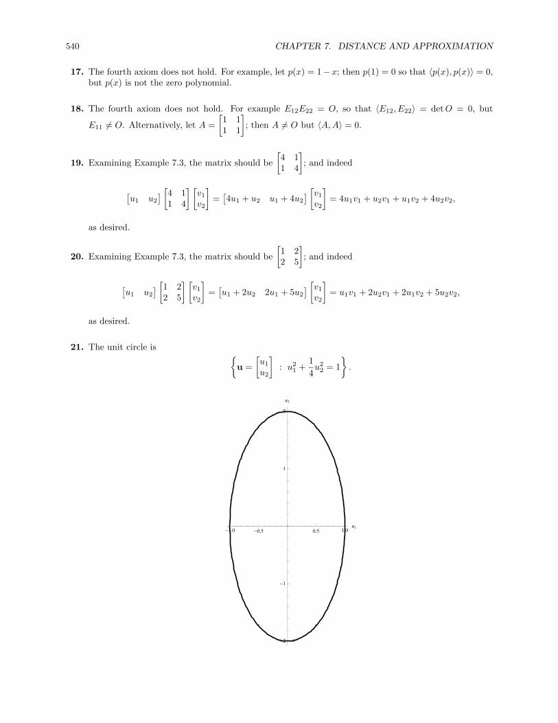
540 CHAPTER 7. DISTANCE AND APPROXIMATION
17. The fourth axiom does not hold. For example, let p(x) = 1− x; then p(1) = 0 so that 〈p(x), p(x)〉 = 0,but p(x) is not the zero polynomial.
18. The fourth axiom does not hold. For example E12E22 = O, so that 〈E12, E22〉 = detO = 0, but
E11 6= O. Alternatively, let A =
[1 11 1
]; then A 6= O but 〈A,A〉 = 0.
19. Examining Example 7.3, the matrix should be
[4 11 4
]; and indeed
[u1 u2
] [4 11 4
] [v1
v2
]=[4u1 + u2 u1 + 4u2
] [v1
v2
]= 4u1v1 + u2v1 + u1v2 + 4u2v2,
as desired.
20. Examining Example 7.3, the matrix should be
[1 22 5
]; and indeed
[u1 u2
] [1 22 5
] [v1
v2
]=[u1 + 2u2 2u1 + 5u2
] [v1
v2
]= u1v1 + 2u2v1 + 2u1v2 + 5u2v2,
as desired.
21. The unit circle is {u =
[u1
u2
]: u2
1 +1
4u2
2 = 1
}.
-1.0 -0.5 0.5 1.0u1
-2
-1
1
2
u2

7.1. INNER PRODUCT SPACES 541
22. The unit circle is {u =
[u1
u2
]: 4u2
1 + 2u1u2 + 4u22 = 1
}.
-0.6 -0.4 -0.2 0.2 0.4 0.6u1
-0.6
-0.4
-0.2
0.2
0.4
0.6
u2
23. We have, using properties of the inner product,
〈u, cv〉 = 〈cv,u〉 (Property 1)
= c 〈v,u〉 (Property 3)
= c 〈u,v〉 (Property 1).
24. Let w be any vector. Then 〈u,0〉 = 〈u, 0w〉 which, by Theorem 7.1(b), is equal to 0 〈u,w〉 = 0.Similarly, 〈0,v〉 = 〈0w,v〉 which, by property 3 of inner products, is equal to 0 〈w,v〉 = 0.
25. Using properties of the inner product and Theorem 7.1 as needed,
〈u + w,v −w〉 = 〈u,v −w〉+ 〈w,v −w〉= 〈u,v〉+ 〈u,−w〉+ 〈w,v〉+ 〈w,−w〉= 〈u,v〉 − 〈u,w〉+ 〈v,w〉 − 〈w,w〉
= 1− 5 + 0− ‖w‖2
= −4− 4 = −8.
26. Using properties of the inner product and Theorem 7.1 as needed,
〈2v −w, 3u + 2w〉 = 〈2v, 3u + 2w〉+ 〈−w, 3u + 2w〉= 〈2v, 3u〉+ 〈2v, 2w〉+ 〈−w, 3u〉+ 〈−w, 2w〉= 6 〈v,u〉+ 4 〈v,w〉 − 3 〈w,u〉 − 2 〈w,w〉
= 6 〈u,v〉+ 4 〈v,w〉 − 3 〈u,w〉 − 2 ‖w‖2
= 6 · 1 + 4 · 0− 3 · 5− 2 · 22 = −17.
27. Using properties of the inner product and Theorem 7.1 as needed,
‖u + v‖ =√〈u + v,u + v〉
=√〈u,u〉+ 〈u,v〉+ 〈v,u〉+ 〈v,v〉
=
√‖u‖2 + 2 〈u,v〉+ ‖v‖2
=√
1 + 2 · 1 + 3 =√
6.

542 CHAPTER 7. DISTANCE AND APPROXIMATION
28. Using properties of the inner product and Theorem 7.1 as needed,
‖2u− 3v + w‖ =√〈2u− 3v + w, 2u− 3v + w〉
=√
4 〈u,u〉 − 12 〈u,v〉 − 6 〈v,w〉+ 4 〈u,w〉+ 9 〈v,v〉+ 〈w,w〉
=
√4 ‖u‖2 − 12 〈u,v〉 − 6 〈v,w〉+ 4 〈u,w〉+ 9 ‖v‖2 + ‖w‖2
=
√4 · 12 − 12 · 1− 6 · 0 + 4 · 5 + 9 ·
(√3)2
+ 22
=√
43.
29. u+v = w means that u+v−w = 0; this is true if and only if 〈u + v −w,u + v −w〉 = 0. Computingthis inner product gives
〈u + v −w,u + v −w〉 = 〈u,u〉+ 2 〈u,v〉 − 2 〈u,w〉 − 2 〈v,w〉+ 〈v,v〉+ 〈−w,−w〉
= ‖u‖2 + 2 · 1− 2 · 5− 2 · 0 + ‖v‖2 + ‖w‖2
= 1 + 2− 10 + 3 + 2 = 0.
30. Since ‖u‖ = 1, we also have 1 = ‖u‖2 = 〈u,u〉. Similarly, 1 = 〈v,v〉. But then
0 ≤ 〈u + v,u + v〉 = 〈u,u〉+ 2 〈u,v〉+ 〈v,v〉 = 2 + 2 〈u,v〉 .
Solving this inequality gives 2 〈u,v〉 ≥ −2, so that 〈u,v〉 ≥ −1.
31. We have
〈u + v,u− v〉 = 〈u,u〉+ 〈u,v〉 − 〈v,u〉 − 〈v,v〉 .
Since inner products are commutative, the middle two terms cancel, leaving us with
〈u,u〉 − 〈v,v〉 = ‖u‖2 − ‖v‖2 .
32. We have
‖u + v‖2 = 〈u + v,u + v〉 = 〈u,u〉+ 〈u,v〉+ 〈v,u〉+ 〈v,v〉 .
Since inner products are commutative, the middle two terms are the same, and we get
〈u,u〉+ 2 〈u,v〉+ 〈v,v〉 = ‖u‖2 + 2 〈u,v〉+ ‖v‖2 .
33. From Exercise 32, we have
‖u + v‖2 = ‖u‖2 + 2 〈u,v〉+ ‖v‖2 . (1)
Substituting −v for v gives another identity,
‖u− v‖2 = ‖u‖2 + 2 〈u,−v〉+ ‖−v‖2 = ‖u‖2 − 2 〈u,v〉+ ‖v‖2 . (2)
Adding these two gives
‖u + v‖2 + ‖u− v‖2 = 2 ‖u‖2 + 2 ‖v‖2 ,
and dividing through by 2 gives the required identity.
34. Solve (1) and (2) in the previous exercise for 〈u,v〉, giving
〈u,v〉 =1
2
(‖u + v‖2 − ‖u‖2 − ‖v‖2
)〈u,v〉 =
1
2
(−‖u− v‖2 + ‖u‖2 + ‖v‖2
).

7.1. INNER PRODUCT SPACES 543
Add these two equations, giving
2 〈u,v〉 =1
2
(‖u + v‖2 − ‖u− v‖2
);
dividing through by 2 gives
〈u,v〉 =1
4
(‖u + v‖2 − ‖u− v‖2
)=
1
4‖u + v‖2 − 1
4‖u− v‖2 .
35. Use Exercise 34. First, if ‖u + v‖ = ‖u− v‖, then Exercise 34 implies that 〈u,v〉 = 0. Second, supposethat u and v are orthogonal. Then again from Exercise 34,
0 =1
4‖u + v‖2 − 1
4‖u− v‖2 =
1
4(‖u + v‖+ ‖u− v‖) (‖u + v‖ − ‖u− v‖) ,
so that one of the two factors must be zero. If the first factor is zero, then both norms are zero, sothey are equal. If the second factor is zero, then we have ‖u + v‖ − ‖u− v‖ = 0 and again the normsare equal.
36. From (2) in Exercise 33, we have
d(u,v) = ‖u− v‖ =
√‖u‖2 − 2 〈u,v〉+ ‖v‖2.
This is equal to
√‖u‖2 + ‖v‖2 if and only if 〈u,v〉 = 0, which is to say when u and v are orthogonal.
37. The inner product we are working with is 〈u,v〉 = 2u1v1 + 3u2v2, so that
v1 =
[10
]v2 =
[11
]− 2 · 1 · 1 + 3 · 1 · 0
2 · 1 · 1 + 3 · 0 · 0
[10
]=
[11
]−[10
]=
[01
].
The orthogonal basis is
{[10
],
[01
]}.
38. The inner product we are working with is
〈u,v〉 = uTAv = uT[
4 −2−2 7
]= 4u1v1 − 2u1v2 − 2u2v1 + 7u2v2.
Then
v1 =
[10
]v2 =
[1
1
]− 4 · 1 · 1− 2 · 1 · 1− 2 · 1 · 0 + 7 · 0 · 1
4 · 1 · 1− 2 · 1 · 0− 2 · 1 · 0 + 7 · 0 · 0
[1
0
]=
[1
1
]− 1
2
[1
0
]=
[12
1
].
39. The inner product we are working with is⟨a0 + a1x+ a2x
2, b0 + b1x+ b2x2⟩
= a0b0 + a1b1 + a2b2.Then
v1 = 1
v2 = (1 + x)− 1 · (1 + x)
1 · 11 = (1 + x)− 1 = x
v3 = (1 + x+ x2)− 1 · (1 + x+ x2)
1 · 11− x · (1 + x+ x2)
x · xx = (1 + x+ x2)− 1− x = x2.
The orthogonal basis is {1, x, x2}.

544 CHAPTER 7. DISTANCE AND APPROXIMATION
40. The inner product we are working with is 〈p(x), q(x)〉 =∫ 1
0p(x)q(x) dx. Then
v1 = 1
v2 = (1 + x)− 1 · (1 + x)
1 · 11 = (1 + x)−
∫ 1
0(1 + x) dx∫ 1
01 dx
1 = (1 + x)− 3
21 = −1
2+ x
v3 = (1 + x+ x2)− 1 · (1 + x+ x2)
1 · 11−
(− 1
2 + x)· (1 + x+ x2)(
− 12 + x
)·(− 1
2 + x) (
−1
2+ x
)= (1 + x+ x2)−
∫ 1
0(1 + x+ x2) dx∫ 1
01 dx
1−∫ 1
0
(− 1
2 + x)
(1 + x+ x2) dx∫ 1
0
(− 1
2 + x)·(− 1
2 + x) (
−1
2+ x
)= (1 + x+ x2)− 11
61− 1/6
1/12
(−1
2+ x
)= (1 + x+ x2)− 11
61− 2
(−1
2+ x
)=
1
6− x+ x2.
41. The inner product here is 〈f, g〉 =∫ 1
−1f(x)g(x) dx.
(a) To normalize the first three Legendre polynomials, we find the norm of each:
‖1‖ =
√∫ 1
−1
1 · 1 dx =
√∫ 1
−1
1 dx =√
2
‖x‖ =
√∫ 1
−1
x · x dx =
√∫ 1
−1
x2 dx =
√[1
3x3
]1
−1
=
√2
3∥∥∥∥x2 − 1
3
∥∥∥∥ =
√∫ 1
−1
(x2 − 1
3
)(x2 − 1
3
)dx =
√∫ 1
−1
(x4 − 2
3x2 +
1
9
)dx
=
√[1
5x5 − 2
9x3 +
1
9x
]1
−1
=2√
2
3√
5.
So the normalized Legendre polynomials are
1
‖1‖=
1√2,
x
‖x‖=
√6
2x,
x2 − 13∥∥x2 − 13
∥∥ =3√
5
2√
2
(x2 − 1
3
)=
√5
2√
2(3x2 − 1).

7.1. INNER PRODUCT SPACES 545
(b) For the computation, we will use the unnormalized Legendre polynomials given in Example 3.8,1, x, and x2 − 1
3 , and normalize the fourth one at the end. With x4 = x3, we have
v4 = x4 −x4 · v1
v1 · v1v1 −
x4 · v2
v2 · v2v2 −
x4 · v3
v3 · v3v3
= x3 −∫ 1
−1x3 · 1 dx∫ 1
−11 · 1 dx
1−∫ 1
−1x3 · x dx∫ 1
−1x · x dx
x−∫ 1
−1x3(x2 − 1
3
)dx∫ 1
−1
(x2 − 1
3
) (x2 − 1
3
)dx
(x2 − 1
3
)
= x3 −∫ 1
−1x3 dx∫ 1
−11 dx
1−∫ 1
−1x4 dx∫ 1
−1x2 dx
x−∫ 1
−1
(x5 − 1
3x3)dx∫ 1
−1
(x4 − 2
3x2 + 1
9
)dx
(x2 − 1
3
)
= x3 −[
14x
4]1−1
21−
[15x
5]1−1[
13x
3]1−1
x−[
16x
6 − 112x
4]1−1[
15x
5 − 29x
3 + 19x]1−1
(x2 − 1
3
)= x3 − 0− 2/5
2/3x− 0
= x3 − 3
5x.
The norm of this polynomial is
‖v4‖ =
√∫ 1
−1
(x3 − 3
5x
)(x3 − 3
5x
)dx =
√∫ 1
−1
(x6 − 6
5x4 +
9
25x2
)dx
=
√[1
7x7 − 6
25x5 +
3
25x3
]1
−1
=2√
14
35.
Thus the normalized Legendre polynomial is
35
2√
14
(x3 − 3
5x
)=
√14
4(5x3 − 3x).
42. (a) Starting with `0(x) = 1, `1(x) = x, `2(x) = x2 − 13 , `3(x) = x3 − 3
5x, we have
`0(1) = 1 ⇒ L0(x) = 1
`1(1) = 1 ⇒ L1(x) = x
`2(1) = 1− 1
3=
2
3⇒ L2(x) =
3
2
(x2 − 1
3
)=
3
2x2 − 1
2
`3(1) = 1− 3
5− 2
5⇒ L3(x) =
5
2
(x3 − 3
5x
)=
5
2x3 − 3
2x.
(b) For L2 and L3, the given recurrence says
L2(x) =2 · 2− 1
2xL1(x)− 2− 1
2L0(x) =
3
2x2 − 1
2
L3(x) =2 · 3− 1
3xL2(x)− 3− 1
3L1(x) =
5
3x
(3
2x2 − 1
2
)− 2
3x =
5
2x3 − 3
2x,
so that the recurrence indeed works for n = 2 and n = 3. Then
L4(x) =2 · 4− 1
4xL3(x)− 4− 1
4L2(x) =
7
4x
(5
2x3 − 3
2x
)− 3
4
(3
2x2 − 1
2
)=
35
8x4 − 15
4x2 +
3
8
L5(x) =2 · 5− 1
5xL4(x)− 5− 1
5L3(x) =
9
5x
(35
8x4 − 15
4x2 +
3
8
)− 4
5
(5
2x3 − 3
2x
)=
63
8x5 − 35
4x3 +
15
8x.

546 CHAPTER 7. DISTANCE AND APPROXIMATION
43. Let B = {ui} be an orthogonal basis for W . Then
〈projW (v),uj〉 =
⟨∑ 〈ui,v〉〈ui,ui〉
ui,uj
⟩=
⟨〈uj ,v〉〈uj ,uj〉
uj ,uj
⟩=〈uj ,v〉〈uj ,uj〉
〈uj ,uj〉 = 〈uj ,v〉 .
Then
〈perpW (v),uj〉 = 〈v − projW (v),uj〉 = 〈v,uj〉 − 〈projW (v),uj〉 = 〈v,uj〉 − 〈uj ,v〉 = 0.
Thus perpW (v) is orthogonal to every vector in B, so that perpW (v) is orthogonal to every w ∈W .
44. (a) We have
〈tu + v, tu + v〉 = t2 〈u,u〉+ 2t 〈u,v〉+ 〈v,v〉 = ‖u‖2 t2 + 2 〈u,v〉 t+ ‖v‖2 ≥ 0.
This is a quadratic at2 + bt+ c in t, where a = ‖u‖2, b = 2 〈u,v〉, and c = ‖v‖2.
(b) Since a = ‖u‖2 > 0, this is an upward-opening parabola, so its vertex is its lowest point. Thatvertex is at − b
2a , so the lowest point, which must be nonnegative, is
a
(− b
2a
)2
+ b
(− b
2a
)+ c =
ab2
4a2− b2
2a+ c =
b2 − 2b2 + 4ac
4a=
4ac− b2
4a≥ 0.
Since 4a > 0, we must have 4ac ≥ b2, so that√ac ≥ 1
2 |b|.
(c) Substituting back in the values of a, b, and c from part (a) gives
√ac =
√‖u‖2 ‖v‖2 = ‖u‖ ‖v‖ ≥ 1
2|b| = 1
2|2 〈u,v〉| = |〈u,v〉| .
Thus ‖u‖ ‖v‖ ≥ |〈u,v〉|, which is the Cauchy-Schwarz inequality.
Exploration: Vectors and Matrices with Complex Entries
1. Recall that if z ∈ C, then zz = |z|2. Then for v as given, we have
‖v‖ =√v · v =
√v1v1 + v2v2 + · · ·+ vnvn =
√|v1|2 + · · ·+ |vn|2.
Finally, we must show that |z|2 =∣∣z2∣∣. But
|z|2 = (zz)2
= zzz2 = z2z2 =∣∣z2∣∣ ,
so the above is in fact equal to√|v2
1 |+ · · ·+ |v2n|.
2. (a) u · v = i · (2− 3i) + 1 · (1 + 5i) = −i(2− 3i) + (1 + 5i) = −2 + 3i.
(b) By Exercise 1, ‖u‖ =√|i2|+ |12| =
√|−1|+ |1| =
√2.
(c) By Exercise 1,
‖v‖ =√|(2− 3i)2|+ |(1 + 5i)2| =
√(2 + 3i)(2− 3i) + (1− 5i)(1 + 5i) =
√13 + 26 =
√39.
(d) d(u,v) = ‖u− v‖ =
∥∥∥∥[−2 + 4i−5i
]∥∥∥∥ =
√|−2 + 4i|2 + |−5i|2 =
√(−2− 4i)(−2 + 4i) + (5i)(−5i) =
3√
5.
Exploration: Vectors and Matrices with Complex Entries 547
(e) If w =
[ab
]is orthogonal to u, then
u ·w = i · a+ 1 · b = −ai+ b = 0,
so that b = ai. Thus for example setting a = 1, we get[1i
].
(f) If w =
[ab
]is orthogonal to v, then
u ·w = 2− 3i · a+ 1 + 5i · b = (2 + 3i)a+ (1− 5i)b = 0.
So b = − 2+3i1−5ia; setting for example a = 1− 5i, we get b = −2− 3i, and one possible vector is[
1− 5i−2− 3i
]
3. (a) v · u = v1u1 + · · ·+ vnun = v1u1 + · · ·+ vnun = v1u1 + · · ·+ vnun = u1v1 + · · ·+ unvn = u · v.(b)
u · (v + w) = u1(v1 + w1) + u2(v2 + w2) + · · ·un(vn + wn)
= u1v1 + u1w1 + u2v2 + u2w2 + · · ·+ unvn + unwn
= (u1v1 + u2v2 + · · ·+ unvn) + (u1w1 + u2w2 + · · ·+ unwn)
= u · v + u ·w.
(c) First,
(cu) · v = cu1v1 + · · ·+ cunvn = cu1v1 + · · ·+ cunvn = c(u1v1 + · · ·+ nnvn) = cu · v.
For the second equality, we have, using part (a),
u · (cv) = (cu) · v = cu · v = cu · v = cv · u.
(d) By Exercise 1, u · u = ‖u‖2 =∣∣u2
1
∣∣ + · +∣∣u2n
∣∣ ≥ 0. Further, equality holds if and only if each∣∣u2i
∣∣ = |ui|2 = 0, so all the ui must be zero and therefore u = 0.
4. Just apply the definition: conjugate A and take its transpose:
(a) A∗ = AT
=
[−i i−2i 3
].
(b) A∗ = AT
=
[2 5− 2i
5 + 2i −1
].
(c) A∗ = AT
=
2 + i 41− 3i 0−2 3 + 4i
.
(d) A∗ = AT
=
−3i 1 + i 1− i0 4 0
1− i −i i
.

548 CHAPTER 7. DISTANCE AND APPROXIMATION
5. These facts follow directly from standard properties of complex numbers together with the fact thatmatrix conjugation is element by element:
(a) A =[aij]
= [aij ] = A.
(b) A+B =[aij + bij
]=[aij + bij
]= [aij ] +
[bij]
= A+B.
(c) cA = [caij ] = [c · aij ] = c [aij ] = cA.
(d) Let C = AB; then cij =∑k aikbkj , so that
ABij = Cij =
[∑k
aikbkj
]ij
=
[∑k
aikbik
]ij
=[A ·B
]ij,
so that AB = A ·B.
(e) The ij entry of(A)T
is aji. The ij entry of AT is aji, so its conjugate, which is the ij entry of
AT , is aji. So the two matrices have the same entries and thus are equal.
6. These facts follow directly from the facts in Exercise 5.
(a) (A∗)∗
=(AT)∗
=(AT)T
=
(AT)T
=(AT)T
= A.
(b) (A+B)∗ = (A+B)T = AT +BT = A∗ +B∗.
(c) (cA)∗ = (cA)T = cAT = cAT = cA∗.
(d) (AB)∗ = (AB)T = BTAT = BT ·AT = B∗A∗.
7. We have u · v =∑uivi =
[u1 u2 · · · un
]v1
v2
...vn
= uTv = u∗v.
8. If A is Hermitian, then aij = aji for all i and j. In particular, when i = j, this gives aii = aii, so thataii is equal to its own conjugate and therefore must be real.
9. (a) A is not Hermitian since it does not have real diagonal entries.
(b) A is not Hermitian since a12 = 2− 3i and a21 = 2− 3i = 2 + 3i; the two are not equal.
(c) A is not Hermitian since a12 = 1− 5i and a21 = −1− 5i; the two are not equal.
(d) A is Hermitian, since every entry is the conjugate of the same entry in its transpose.
(e) A is not Hermitian. Since it is a real matrix, it is equal to its conjugate, but AT 6= A since A isnot symmetric.
(f) A is Hermitian. Since it is a real matrix, it is equal to its conjugate, and it is symmetric, so that
AT
= AT = A.
10. Suppose that λ is an eigenvalue of a Hermitian matrix A, with corresponding eigenvector v. Now,
v∗A = v∗A∗ = (Av)∗ = (λv)∗
since A is Hermitian. But by Exercise 6(c), (λv)∗ = λv∗. Then
λ(v∗v) = v∗(λv) = v∗(Av) = (v∗A)v =(λv∗
)v = λ(v∗v).
Then since v 6= 0, we have by Exercise 7 v∗v = v ·v = ‖v‖2 6= 0. So we can divide the above equationthrough by v∗v to get λ = λ, so that λ is real.

Exploration: Vectors and Matrices with Complex Entries 549
11. Following the hint, adapt the proof of Theorem 5.19. Suppose that λ1 6= λ2 are eigenvalues of aHermitian matrix A corresponding to eigenvectors v1 and v2 respectively. Then
λ1(v1 · v2) = (λ1v1) · v2 = (Av1) · v2 = (Av1)∗v2 = (v∗1A∗)v2.
But A is Hermitian, so A∗ = A and we continue:
(v∗1A∗)v2 = (v∗1A)v2 = v∗1(Av2) = v∗1(λ2v2) = λ2(v∗1v2) = λ2(v1 · v2).
Thus λ1(v1 · v2) = λ2(v1 · v2), so that (λ1 − λ2)(v1 · v2) = 0. But λ1 6= λ2 by assumption, so we musthave v1 · v2 = 0.
12. (a) Multiplying, we get AA∗ = I, so that A is unitary and A−1 = A∗ =
[− i√
2− i√
2i√2− i√
2
].
(b) Multiplying, we get AA∗ =
[4 00 4
]6= I, so that A is not unitary.
(c) Multiplying, we get AA∗ = I, so that A is unitary and A−1 = A∗ =
[35 − 4i
5
− 45 − 3i
5
].
(d) Multiplying, we get AA∗ = I, so that A is unitary and A−1 = A∗ =
1−i√
60 −1+i√
3
0 1 02√6
0 1√3
.
13. First show (a) ⇔ (b). Let ui denote the ith column of a matrix U . Then the ith row of U∗ is ui. Thenby the definition of matrix multiplication,
(U∗U)ij = ui · uj .
Then the columns of U form an orthonormal set if and only if
ui · uj =
{0 i 6= j
1 i = j,
which holds if and only if
(U∗U)ij =
{0 i 6= j
1 i = j,
which is to say that U∗U = I. Thus the columns of U are orthogonal if and only if U is unitary.
Now apply this to the matrix U∗. We get that U∗ is unitary if and only if the columns of U∗ areorthogonal. But U∗ is unitary if and only if U is, since
(U∗)∗U∗ = UU∗,
and the columns of U∗ are just the conjugates of the rows of U , so that (letting Ui be the ith row ofU)
Ui · Uj = Ui∗Uj = (Ui)
TUj = Uj · Ui.
So the columns of U∗ are orthogonal if and only if the rows of U are orthogonal. This proves (a) ⇔(c).
Next, we show (a) ⇒ (e) ⇒ (d) ⇒ (e) ⇒ (a). To prove (a) ⇒ (e), assume that U is unitary. ThenU∗U = I, so that
Ux · Uy = (Ux)∗Uy = x∗U∗Uy = x∗y = x · y.

550 CHAPTER 7. DISTANCE AND APPROXIMATION
Next, for (e) ⇒ (d), assume that (e) holds. Then Qx · Qx = x · x, so that ‖Qx‖ =√Qx ·Qx =√
x · x = ‖x‖. Next, we show (d) ⇒ (e). Let ui denote the ith column of U . Then
x · y =1
4
(‖x + y‖2 − ‖x− y‖2
)=
1
4
(‖U(x + y)‖2 − ‖U(x− y)‖2
)=
1
4
(‖Ux + Uy‖2 − ‖Ux− Uy‖2
)= Ux · Uy.
Thus (d) ⇒ (e). Finally, to see that (e) ⇒ (a), let ei be the ith standard basis vector. Then ui = Uei,so that since (e) holds,
ui · uj = Uei · Uej = ei · ej =
{0 i 6= j
1 i = j.
This shows that the columns of U form an orthonormal set, so that U is unitary.
14. (a) Since
[i√2i√2
]·
[− i√
2i√2
]= − i√
2·(− i√
2
)− i√
2· i√
2= 0
[i√2i√2
]·
[i√2i√2
]= − i√
2· i√
2− i√
2· i√
2= 1
[− i√
2i√2
]·
[− i√
2i√2
]=
i√2·(− i√
2
)− i√
2· i√
2= 1,
the columns of the matrix are orthonormal, so the matrix is unitary.
(b) The dot product of the first column with itself is
1 + i(1 + i) + 1− i(1− i) = (1− i)(1 + i) + (1 + i)(1− i) = 4 6= 1,
so that the matrix is not unitary.
(c) Since
[354i5
]·
[− 4
53i5
]=
3
5·(−4
5
)− 4i
5· 3i
5= 0[
354i5
]·
[354i5
]=
3
5· 3
5− 4i
5· 4i
5= 1[
− 45
3i5
]·
[− 4
53i5
]= −4
5·(−4
5
)− 3i
5· 3i
5= 1,
the columns of the matrix are orthonormal, so the matrix is unitary.

Exploration: Vectors and Matrices with Complex Entries 551
(d) Clearly column 2 is a unit vector, and is orthogonal to each of the other two columns, so we needonly show the first and third columns are unit vectors and are orthogonal. But
1+i√6
0−1−i√
3
·
2√6
01√3
=1− i√
6· 2√
6+ 0 +
−1 + i√3· 1√
3=
2− 2i
6+−1 + i
3= 0
1+i√
6
0−1−i√
3
·
1+i√6
0−1−i√
3
=1− i√
6· 1 + i√
6+ 0 +
−1 + i√3· −1− i√
3=
2
6+
2
3= 1
2√6
01√3
·
2√6
01√3
=2√6· 2√
6+ 0 +
1√3· 1√
3=
4
6+
1
3= 1,
and we are done.
15. (a) With A as given, the characteristic polynomial is (λ−2)2− i · (−i) = λ2−4λ+ 3 = (λ−1)(λ−3).Thus the eigenvalues are λ1 = 1 and λ2 = 3. Corresponding eigenvectors are
λ = 1 :
[1i
], λ = 3 :
[1 + i1− i
].
Since these eigenvectors correspond to different eigenvalues, they are already orthogonal. Theirnorms are ∥∥∥∥[1i
]∥∥∥∥ =√
1 · 1 + (−i) · i =√
2,
∥∥∥∥[1 + i1− i
]∥∥∥∥ =
√|1 + i|2 + |1− i|2 = 2.
So defining a matrix U whose columns are the normalized eigenvectors gives
U =
[1√2
1+i2
i√2
1−i2
],
which is unitary. Then
U∗AU =
[1 00 3
].
(b) With A as given, the characteristic polynomial is λ2 + 1. Thus the eigenvalues are λ1 = i andλ2 = −i. Corresponding eigenvectors are
λ = 1 :
[i1
], λ = 3 :
[−i1
].
Since these eigenvectors correspond to different eigenvalues, they are already orthogonal. Theirnorms are ∥∥∥∥[i1
]∥∥∥∥ =
√|i|2 + |1|2 =
√2,
∥∥∥∥[−i1]∥∥∥∥ =
√|−i|2 + |1|2 =
√2.
So defining a matrix U whose columns are the normalized eigenvectors gives
U =
[i√2− i√
21√2
1√2
],
which is unitary. Then
U∗AU =
[i 00 −i
].

552 CHAPTER 7. DISTANCE AND APPROXIMATION
(c) With A as given, the characteristic polynomial is (λ+1)λ−(1+i)(1−i) = λ2+λ−2 = (λ+2)(λ−1).Thus the eigenvalues are λ1 = 1 and λ2 = −2. Corresponding eigenvectors are
λ = 1 :
[1 + i
2
], λ = 3 :
[1 + i−1
].
Since these eigenvectors correspond to different eigenvalues, they are already orthogonal. Theirnorms are ∥∥∥∥[1 + i
2
]∥∥∥∥ =
√|1 + i|2 + |2|2 =
√6,
∥∥∥∥[1 + i−1
]∥∥∥∥ =
√|1 + i|2 + |1|2 =
√3.
So defining a matrix U whose columns are the normalized eigenvectors gives
U =
[1+i√
61+i√
32√6− 1√
3
],
which is unitary. Then
U∗AU =
[1 00 −2
].
(d) With A as given, the characteristic polynomial is
(λ− 1) ((λ− 2)(λ− 3)− (1− i)(1 + i)) = (λ− 1)(λ2 − 5λ+ 4
)= (λ− 1)2(λ− 4)
Thus the eigenvalues are λ1 = 1 and λ2 = 4. Corresponding eigenvectors are
λ = 1 :
0−1 + i
1
,1
00
, λ = 4 :
01− i
2
.The eigenvectors corresponding to different eigenvalues are already orthogonal, and the two eigen-vectors corresponding to λ = 1 are also orthogonal, so these vectors form an orthogonal set. Theirnorms are ∥∥∥∥∥∥
0−1 + i
1
∥∥∥∥∥∥ =
√|0|2 + |−1 + i|2 + |1|2 =
√3,
∥∥∥∥∥∥1
00
∥∥∥∥∥∥ = 1,
∥∥∥∥∥∥ 0
1− i2
∥∥∥∥∥∥ =
√|0|2 + |1− i|2 + |2|2 =
√6.
So defining a matrix U whose columns are the normalized eigenvectors gives
U =
0 1 0−1+i√
30 1−i√
61√3
0 2√6
,which is unitary. Then
U∗AU =
1 0 00 1 00 0 4
.16. If A is Hermitian, then A∗ = A, so that A∗A = AA = AA∗. Next, if U is unitary, then UU∗ = I. But if
U is unitary, then its rows are orthonormal. Since the columns of U∗ are the conjugates of the rows ofU , they are orthonormal as well and therefore U∗ is also unitary. Hence UU∗ = U∗U = I and thereforeU is normal. Finally, if A is skew-Hermitian, then A∗ = −A; then A∗A = −AA = A(−A) = AA∗. Soall three of these types of matrices are normal.
17. By the result quoted just before Exercise 16, if A is unitarily diagonalizable, then A∗A = AA∗; this isthe definition of A being normal.

Exploration: Geometric Inequalities and Optimization Problems 553
Exploration: Geometric Inequalities and Optimization Problems
1. We have
|u · v| =√x · √y +
√y ·√x = 2
√x√y
‖u‖ = ‖v‖ =
√(√x)2
+ (√y)
2=√x+ y,
so that 2√x√y ≤√x+ y ·
√x+ y = x+ y, and thus
√xy ≤ x+ y
2.
2. (a) Since(√x−√y
)2is a square, it is nonnegative. Expanding then gives x − 2
√x√y + y ≥ 0, so
that 2√xy ≤ x+ y and thus
√xy ≤ x+ y
2.
(b) Let AD = a and BD = b. Then by the Pythagorean Theorem,
CD2 = a2 − x2 = b2 − y2,
so that 2CD2 = (a2 + b2)− x2 − y2 = (x+ y)2 − (x2 + y2) = 2xy, so that CD =√xy. But CD
is clearly at most equal to a radius of the circle, since it extends from a diameter to the circle.Since the radius is x+y
2 , we again get
√xy ≤ x+ y
2.
3. Since the area is xy = 100, we have 10 =√xy ≤ x+y
2 , so that 40 ≤ 2(x + y), which is the perimeter.By the AMGM, equality holds when x = y; that is, when x = y = 10, so the square of side 10 is therectangle with smallest perimeter.
4. Let 1x play the role of y in the AMGM. Then√
x · 1
x≤x+ 1
x
2, or 2
√1 = 2 ≤ x+
1
x.
Equality holds if and only if x = 1x , i.e., when x = 1. Thus 1 + 1
1 = 2 is the minimum value for f(x)for x > 0.
5. If the dimensions of the cut-out square are x×x, then the base of the box will be (10−2x)× (10−2x),so its volume will be x(10− 2x)2. Then
3√V ≤ x+ (10− 2x) + (10− 2x)
3=
20− 3x
3,
with equality holding if x = 10 − 2x. Thus x = 103 , so that 10 − 2x = 10
3 as well. Then the largestpossible volume is 10
3 ×103 ×
103 .
6. We have3√f =
(x+ y) + (y + z) + (z + x)
3=
2
3(x+ y + z),
with equality holding if x + y = y + z = z + x. But this implies that x = y = z; since xyz = 1, wemust have x = y = z = 1, so that f(x, y, z) = (1 + 1)(1 + 1)(1 + 1) = 8. This is the minimum value off subject to the constraint xyz = 1.

554 CHAPTER 7. DISTANCE AND APPROXIMATION
7. Use the substitution u = x− y. Then the original expression becomes
u+ y +8
uy.
Using the AMGM for three variables, we get
3
√u · y · 8
uy≤u+ y + 8
uy
3, or 3
3√
8 = 6 ≤ u+ y +8
uy,
with equality holding if and only if u = y = 8uy ; this implies that u = y = 2, so that x = u+ y = 4. So
the minimum values is 4 + 82·2 = 6, which occurs when x = 4 and y = 2.
8. Follow the method of Example 7.11. x2 + 2y2 + z2 is the square of the norm of v =
x√2 yz
, so that
x + 2y + 4z is the dot product of that vector with u =
1√2
4
. Then the component-wise form of the
Cauchy-Schwarz Inequality gives
(1 ·x+√
2 ·√
2 y+4 ·z)2 = (x+2y+4z)2 ≤(
12 +(√
2)2
+ 42
)(x2 +2y2 +z2) = 19(x2 +2y2 +z2) = 19.
So x+ 2y + 4z ≤√
19, and the maximum value is√
19.
9. Follow the method of Example 7.11. Here f(x, y, z) is the square of the norm of v =
xyz√2
, so set
u =
11√2
. Then the component-wise form of the Cauchy-Schwarz Inequality gives
11√2
· xyz√2
2
= (x+ y + z)2 ≤(
12 + 12 +(√
2)2)(
x2 + y2 +1
2z2
).
Since x+ y + z = 10, we get
100le4
(x2 + y2 +
1
2z2
), or 25 ≤ x2 + y2 +
1
2z2.
Thus the minimum value of the function is 25.
10. Follow the method of Example 7.11 with u =
[11
]and v =
[sin θcos θ
]. (This works because ‖v‖2 =
sin2 θ + cos2 θ = 1.) Then the component-wise form of the Cauchy-Schwarz Inequality gives
(u · v)2 = (sin θ + cos θ)2 ≤ (12 + 12)(sin2 θ + cos2 θ) = 2.
Therefore sin θ + cos θ ≤√
2, so the maximum value of the expression is√
2.
11. We want to minimize x2 + y2 subject to the constraint x + 2y = 5. Thus set v =
[xy
]and u =
[12
].
Then the component-wise form of the Cauchy-Schwarz Inequality gives
(x+ 2y)2 ≤ (12 + 22)(x2 + y2).

Exploration: Geometric Inequalities and Optimization Problems 555
Since x+ 2y = 5, we get25 ≤ 5(x2 + y2), or 5 ≤ x2 + y2.
Thus the minimum value is 5, which occurs at equality. To find the point where equality occurs,substitution 5− 2y for x to get
5 = (5− 2y)2 + y2 = 25− 20y + 5y2, so that y2 − 4y + 4 = 0.
This has the solution y = 2; then x = 5 − 2y = 1. So the point on x + 2y = 5 closest to the origin is(1, 2).
12. To show that√xy ≥ 2
1/x+1/y , apply the AMGM to x′ = 1x and y′ = 1
y , giving
√x′y′ ≤ x′ + y′
2, or
√1
x′y′≥ 2
x′ + y′, or
√xy ≥ 2
1/x+ 1/y.
Since this inequality results from the AMGM, we have equality when x′ = y′, so when x = y. For thefirst inequality, note first that (x− y)2 = x2 − 2xy + y2 ≥ 0, so that x2 + y2 ≥ 2xy. Then
x2 + y2
2=x2 + y2 + (x2 + y2)
4≥ x2 + 2xy + y2
4=
(x+ y
2
)2
, so that
√x2 + y2
2≥ x+ y
2.
Equality occurs when x2 + y2 = 2xy, which is the same as (x− y)2 = 0, so that x = y.
13. The area of the rectangle shown is 2xy, where x2 + y2 = r2. From Exercise 12, we have√x2 + y2
2≥ √xy ⇒
√x2 + y2 ≥
√2xy ⇒
√r2 = r ≥
√2xy =
√A ⇒ A ≤ r2.
The maximum occurs at equality, and the maximum area is A = r2. By Exercise 12, this happenswhen x = y.
14. Following the hint, we have(x+ y)2
xy= (x+ y)
(1
x+
1
y
).
So from Exercise 12, we have
x+ y
2≥ 2
1/x+ 1/y⇒ (x+ y)
(1
x+
1
y
)≥ 4.
Thus the minimum value is 4; this minimum occurs when x = y, so when
(x+ x)
(1
x+
1
x
)=
4x
x= 4,
or x = y = 1.
15. Squaring the inequalities in Exercise 12 gives
x2 + y2
2≥(x+ y
2
)2
≥(
2
1/x+ 1/y
)2
.
Substituting x+ 1x for x and y + 1
y for y gives from the first inequality
(x+ 1
x
)2+(y + 1
y
)2
2≥
(x+ 1x
)+(y + 1
y
)2
2
.
556 CHAPTER 7. DISTANCE AND APPROXIMATION
Since the constraint we are working with is x+ y = 1, we get(x+ 1x
)+(y + 1
y
)2
2
=
(x+ y) +(
1x + 1
y
)2
2
=
(1
2+
1x + 1
y
2
)2
≥(
1
2+
2
x+ y
),
using the second and fourth terms in Exercise 12 for the final inequality. But now again since x+y = 1,we get (
1
2+
2
x+ y
)2
=
(5
2
)2
=25
4,
so that f(x, y) = 2 · 254 = 25
2 is the minimum when x+ y = 1. This equality holds when x = y, so thatx = y = 1
2 .
7.2 Norms and Distance Functions
1. We have
‖u‖E =√
(−1)2 + 42 + (−5)2 =√
42
‖u‖s = |−1|+ |4|+ |−5| = 10
‖u‖m = max (|−1| , |4| , |−5|) = 5.
2. We have
‖v‖E =√
22 + (−2)2 + 02 = 2√
2
‖v‖s = |2|+ |−2|+ |0| = 4
‖v‖m = max (|2| , |−2| , |0|) = 2.
3. u− v =
−36−5
, so
dE(u,v) =√
(−3)2 + 62 + (−5)2 =√
70
ds(u,v) = |−3|+ |6|+ |−5| = 14
dm(u,v) = max (|−3| , |6| , |−5|) = 6.
4. (a) ds(u,v) measures the total difference in magnitude between corresponding components.
(b) dm(u,v) measure the greatest difference between any pair of corresponding components.
5. ‖u‖H = w(u), which is the number of 1s in u, or 4. ‖v‖H = w(v), which is the number of 1s in v, or5.
6. dH(u,v) = w(u− v) = w(u) + w(v) less twice the overlap, or 4 + 5− 2 · 2 = 5; this is the number of1s in u− v.
7. (a) If ‖v‖E =√∑
v2i = max{|vi|} = ‖v‖m, then squaring both sides gives
∑v2i = max{|vi|2} =
max{v2i }. Since v2
i ≥ 0 for all i, equality holds if and only if exactly one of the vi is nonzero.
(b) Suppose ‖v‖s =∑|vi| = max{|vi|} = ‖v‖m. Since |vi| ≥ 0 for all i, equality holds if and only if
exactly one of the vi is nonzero.
(c) By parts (a) and (b), ‖v‖E = ‖v‖m = ‖v‖s if and only if exactly one of the components of v isnonzero.

7.2. NORMS AND DISTANCE FUNCTIONS 557
8. (a) Since
‖u + v‖E =∑
(ui + vi)2 =
∑u2i +
∑v2i + 2
∑uivi = ‖u‖E + ‖v‖E + 2u · v,
we see that ‖u + v‖E = ‖u‖E + ‖v‖E if and only if u · v = 0; that is, if and only if u and v areorthogonal.
(b) We have
‖u + v‖s =∑|ui + vi| , ‖u‖s + ‖v‖s =
∑(|ui|+ |vi|).
For a given i, if the signs of ui and vi are the same, then |ui + vi| = |ui| + |vi|, while if they aredifferent, then |ui + vi| < |ui|+ |vi|. Thus the two norms are equal exactly when ui and vi havethe same sign for each i, which is to say that uivi ≥ 0 for all i.
(c) We have
‖u + v‖s = max{|ui + vi|}, ‖u‖s + ‖v‖s = max{|ui|}+ max{|vi|}.
Suppose that |ur| = max{|ui|} and |vt| = max{|vi|}. Then for any j, we know that
|uj + vj | ≤ |uj |+ |vj | ≤ |ur|+ |vt| ,
where the first inequality is the triangle inequality and the second comes from the condition on rand t. Choose j such that |uj + vj | = ‖u + v‖s. If the two norms are equal, then
|uj + vj | = ‖u + v‖s = ‖u‖s + ‖v‖s = |ur|+ |vt| .
Thus both of the inequalities above must be equalities. The first is an equality if uj and vj havethe same sign. For the second, since |uj | ≤ |ur| and |vj | ≤ |vt|, equality means that |uj | = |ur| and|vj | = |vt|. Putting this together gives the following (somewhat complicated) condition for equalityto hold in the triangle inequality for the max norm: equality holds if there is some component jsuch that uj and vj have the same sign and such that |uj | is a component of maximal magnitudeof u and |vj | is a component of maximal magnitude of v.
9. Let vk be a component of v with maximum magnitude. Then the result follows from the string ofequalities and inequalities
‖v‖m = |vk| =√v2k ≤
√∑v2i = ‖v‖E .
10. We have ‖v‖2E =∑v2i ≤ (
∑|vi|)2 ≤ ‖v‖2s. Taking square roots gives the desired result since norms
are always nonnegative.
11. We have ‖v‖s =∑|vi| ≤
∑max{|vi|} = nmax{|vi|} = n ‖v‖m.
12. We have ‖v‖E =√∑
v2i ≤
√∑(max{vi})2
=
√nmax{|vi|2} =
√nmax{|vi|} =
√n ‖v‖m.
13. The unit circle in R2 relative to the sum norm is
{(x, y) : |x|+ |y| = 1} = {(x, y) : x+ y = 1 or x− y = 1 or − x+ y = 1 or − x− y = 1}.
The unit circle in R2 relative to the max norm is
{(x, y) : max{|x| , |y|} = 1}.

558 CHAPTER 7. DISTANCE AND APPROXIMATION
These unit circles are shown below:
-1.0 -0.5 0.5 1.0
-1.0
-0.5
0.5
1.0
-1.0 -0.5 0.5 1.0
-1.0
-0.5
0.5
1.0
14. For example, in R2, let u = 〈2, 1〉 and v = 〈1, 2〉. Then ‖u‖ = ‖v‖ = 2 + 1 = 3. Also, ‖u + v‖ =‖〈3, 3〉‖ = 6 and ‖u− v‖ = ‖〈1,−1〉‖ = 2. But then
‖u‖2 + ‖v‖2 = 32 + 32 = 18 6= 1
2‖u + v‖2 +
1
2‖u− v‖2 = 18 + 2 = 20.
15. Clearly
∥∥∥∥[ab]∥∥∥∥ ≥ 0, and since max{|2a| , |3b|} = 0 if and only if both a and b are zero, we see that the
norm is zero only for the zero vector. Thus property (1) is satisfied. For property 2,∥∥∥∥c [ab]∥∥∥∥ =
∥∥∥∥[cacb]∥∥∥∥ = max{|2ac| , |3bc|} = |c|max{|2a| , |3b|}.
Finally, ∥∥∥∥[ab]
+
[cd
]∥∥∥∥ =
∥∥∥∥[a+ cb+ d
]∥∥∥∥ = max{|2(a+ c)| , |3(b+ d)|}.
Now use the triangle inequality:
max{|2(a+ c)| , |3(b+ d)|} ≤ max{|2a|+ |2c| , |3b|+ |3d|} ≤ max{|2a| , |3b|}+ max{|2c| , |3d|}.
But the last expression is just
∥∥∥∥[ab]∥∥∥∥+
∥∥∥∥[cd]∥∥∥∥, and we are done.
16. Clearly maxi,j{|aij |} ≥ 0, and is zero only when all of the aij are zero, so when A = O. Thus property
(1) is satisfied. For property (2),
‖cA‖ = maxi,j{|caij |} = max
i,j{|c| |aij |} = |c|max
i,j{|aij |} = |c| ‖A‖ .
For property (3), using the triangle inequality for absolute values gives
‖A+B‖ = maxi,j{|aij + bij |} ≤ max
i,j{|aij |+ |bij |} ≤ max
i,j{|aij |}+ max
i,j{|bij |} = ‖A‖+ ‖B‖ .
7.2. NORMS AND DISTANCE FUNCTIONS 559
17. Clearly ‖f‖ ≥ 0, since |f | ≥ 0. Since f is continuous, |f | is also continuous, so its integral is zero ifand only if it is identically zero. So property (1) holds. For property (2), use standard properties ofintegrals:
‖cf‖ =
∫ 1
0
|cf(x)| dx =
∫ 1
0
|c| · |f(x)| dx = |c|∫ 1
0
|f(x)| dx = |c| ‖f‖ .
Finally, property (3) relies on the triangle inequality for absolute value:
‖f + g‖ =
∫ 1
0
|f(x) + g(x)| dx ≤∫ 1
0
(|f(x)|+ |g(x)|) dx =
∫ 1
0
|f(x)| dx+
∫ 1
0
|g(x)| dx = ‖f‖+ ‖g‖ .
18. Since the norm is the maximum of a set of nonnegative numbers, it is always nonnegative, and is zeroexactly when all of the numbers are zero, which means that f is the zero function on [0, 1]. So property(1) holds. For property (2), we have
‖cf‖ = max0≤x≤1
{|cf(x)|} = max0≤x≤1
{|c| |f(x)|} = |c| max0≤x≤1
{|f(x)|} = |c| ‖f‖ .
Finally, property (3) relies on the triangle inequality for absolute values:
‖f + g‖ = max0≤x≤1
{|f(x) + g(x)|} ≤ max0≤x≤1
{|f(x)|+|g(x)|} ≤ max0≤x≤1
{|f(x)|}+ max0≤x≤1
{|g(x)|} = ‖f‖+‖g‖ .
19. By property (2) of the definition of a norm,
d(u,v) = ‖u− v‖ = |−1| ‖u− v‖ = ‖(−1)(u− v)‖ = ‖v − u‖ = d(v,u).
20. The Frobenius norm is ‖A‖F =√
22 + 32 + 42 + 12 =√
30. From Theorem 7.7 and the commentfollowing, ‖A‖1 is the largest column sum of |A|, which is 2 + 4 = 6, while ‖A‖∞ is the largest rowsum of |A|, which is 2 + 3 = 4 + 1 = 5.
21. The Frobenius norm is ‖A‖F =√
02 + (−1)2 + (−3)2 + 32 =√
19. From Theorem 7.7 and the com-ment following, ‖A‖1 is the largest column sum of |A|, which is |−1|+ 3 = 4, while ‖A‖∞ is the largestrow sum, which is |−3|+ 3 = 6.
22. The Frobenius norm is ‖A‖F =√
12 + 52 + (−2)2 + (−1)2 =√
31. From Theorem 7.7 and the com-ment following, ‖A‖1 is the largest column sum of |A|, which is 5 + |−1| = 6, while ‖A‖∞ is the largestrow sum, which is 1 + 5 = 6.
23. The Frobenius norm is ‖A‖F =√
22 + 12 + 12 + 12 + 32 + 22 + 12 + 12 + 32 =√
31. From Theorem7.7 and the comment following, ‖A‖1 is the largest column sum of |A|, which is 1 + 2 + 3 = 6, while‖A‖∞ is the largest row sum, which is 1 + 3 + 2 = 6.
24. The Frobenius norm is ‖A‖F =√
02 + (−5)2 + 22 + 32 + 12 + (−3)2 + (−4)2 + (−4)2 + 32 =√
89.From Theorem 7.7 and the comment following, ‖A‖1 is the largest column sum of |A|, which is |−5|+1 + |−4| = 10, while ‖A‖∞ is the largest row sum, which is |−4|+ |−4|+ 3 = 11.
25. The Frobenius norm is ‖A‖F =√
42 + (−2)2 + (−1)2 + 02 + (−1)2 + 22 + 32 + (−3)2 + 02 =√
44 =
2√
11. From Theorem 7.7 and the comment following, ‖A‖1 is the largest column sum of |A|, which is4 + 0 + 3 = 7, while ‖A‖∞ is the largest row sum, which is 4 + |−2|+ |−1| = 7.
26. Since ‖A‖1 = 6, which is the sum of the first column, such a vector x is e1, since[2 34 1
] [10
]=
[24
], and
∥∥∥∥[24]∥∥∥∥
s
= 6.
Since ‖A‖∞ = 5, which is the sum of (say) the first row, let y =
[11
]; then[
2 34 1
] [11
]=
[55
], and
∥∥∥∥[55]∥∥∥∥
m
= 5.
560 CHAPTER 7. DISTANCE AND APPROXIMATION
27. Since ‖A‖1 = 4, which is the sum of the magnitudes of the second column, such a vector x is e2, since[0 −1−3 3
] [01
]=
[−1
3
], and
∥∥∥∥[−13
]∥∥∥∥s
= |−1|+ 3 = 4.
Since ‖A‖∞ = 6, which is the sum of the magnitudes of the second row, let y =
[−1
1
]since the first
column in that row is negative; then[0 −1−3 3
] [−1
1
]=
[−1
6
], and
∥∥∥∥[−16
]∥∥∥∥m
= 6.
28. Since ‖A‖1 = 6, which is the sum of the magnitudes of the second column, such a vector x is e2, since[1 5−2 −1
] [01
]=
[5−1
], and
∥∥∥∥[ 5−1
]∥∥∥∥s
= 5 + |−1| = 6.
Since ‖A‖∞ = 6, which is the sum of the first row, let y =
[11
]; then
[1 5−2 −1
] [11
]=
[6−3
], and
∥∥∥∥[ 6−3
]∥∥∥∥m
= 6.
29. Since ‖A‖1 = 6, which is the sum of the magnitudes of the third column, such a vector x is e3, since2 1 11 3 21 1 3
001
=
123
, and
∥∥∥∥∥∥1
23
∥∥∥∥∥∥s
= 6.
Since ‖A‖∞ = 6, which is the sum of the second row, let y =
111
; then
2 1 11 3 21 1 3
111
=
465
, and
∥∥∥∥∥∥4
65
∥∥∥∥∥∥m
= 6.
30. Since ‖A‖1 = 10, which is the sum of the magnitudes of the second column, such a vector x is e2, since 0 −5 23 1 −3−4 −4 3
010
=
−51−4
, and
∥∥∥∥∥∥−5
1−4
∥∥∥∥∥∥s
= 10.
Since ‖A‖∞ = 11, which is the sum of the magnitudes of the third row, let y =
−1−1
1
since the entries
in the first two columns are negative; then 0 −5 23 1 −3−4 −4 3
−1−1
1
=
7−711
, and
∥∥∥∥∥∥ 7−711
∥∥∥∥∥∥m
= 11.
31. Since ‖A‖1 = 7, which is the sum of the magnitudes of the first column, such a vector x is e1, since4 −2 −10 −1 23 −3 0
100
=
403
, and
∥∥∥∥∥∥4
03
∥∥∥∥∥∥s
= 7.

7.2. NORMS AND DISTANCE FUNCTIONS 561
Since ‖A‖∞ = 7, which is the sum of the magnitudes of the first row, let y =
1−1−1
since the entries
in the last two columns are negative; then4 −2 −10 −1 23 −3 0
1−1−1
=
7−1
6
, and
∥∥∥∥∥∥ 7−1
6
∥∥∥∥∥∥m
= 7.
32. Let Ai be the ith row of A, let M = maxj=1,2,...,n
{‖Aj‖s} be the maximum absolute row sum, and let x
be any vector with ‖x‖m = 1 (which means that |xi| ≤ 1 for all i). Then
‖Ax‖m = maxi{|Aix|}
= maxi{|ai1x1 + ai2x2 + · · ·+ ainxn|}
≤ maxi{|ai1| |x1|+ |ai2| |x2|+ · · ·+ |ai1| |xn|}
≤ maxi{|ai1|+ |ai2|+ · · ·+ |ain|}
= maxi{‖Ai‖s} = M.
Thus ‖Ax‖m is at most equal to the maximum absolute row sum. Next, we find a specific unit vectorx so that it is actually equal to M . Let row k be the row of A that gives the maximum sum norm;that is, such that ‖Ak‖s = M . Let
yj =
{1 Akj ≥ 0
−1 Akj < 0, j = 1, 2, . . . , n.
Then with y =[y1 · · · yn
]T, we have ‖y‖m = 1, and we have corrected any negative signs in row
k, so that akjyj ≥ 0 for all j and therefore the kth entry of Ay is∑j
akjyj =∑j
|akjyj | =∑j
|akj | |yj | =∑j
|akj | = ‖Ak‖s = M.
So we have shown that the ∞ norm of A is bounded by the maximum row sum, and then found avector x for which ‖Ax‖ ≤ ‖A‖∞ is equal to the maximum row sum. Thus ‖A‖∞ is equal to themaximum row sum, as desired.
33. (a) If ‖·‖ is an operator norm, then ‖I‖ = max‖x̂‖=1
‖Ix̂‖ = max‖x̂‖=1
‖x̂‖ = 1.
(b) No, there is not, for n > 1, since in the Frobenius norm, ‖I‖F =√∑
12 =√n 6= 1. When n = 1,
the Frobenius norm is the same as the absolute value norm on the real number line.
34. Let λ be an eigenvalue, and v a corresponding unit vector. Normalize v to v̂. Then Av̂ = λv̂, so that
‖A‖ = max‖x̂‖=1
‖Ax̂‖ ≥ ‖Av̂‖ = ‖λv̂‖ = |λ| ‖v̂‖ = |λ| .
35. Computing the inverse gives
A−1 =
[1 − 1
2
−2 32
].
Then
cond1(A) = ‖A‖1∥∥A−1
∥∥1
= (3 + 4) (1 + |−2|) = 21
cond∞(A) = ‖A‖∞∥∥A−1
∥∥∞ = (4 + 2)
(|−2|+ 3
2
)= 21.
The matrix is well-conditioned.

562 CHAPTER 7. DISTANCE AND APPROXIMATION
36. Since detA = 0, by definition cond1(A) = cond∞(A) =∞, so this matrix is ill-conditioned.
37. Computing the inverse gives
A−1 =
[100 −99−100 100
].
Then
cond1(A) = ‖A‖1∥∥A−1
∥∥1
= (1 + 1)(100 + |−100|) = 400
cond∞(A) = ‖A‖∞∥∥A−1
∥∥∞ = (1 + 1)(100 + |−100|) = 400.
The matrix is ill-conditioned.
38. Computing the inverse gives
A−1 =
[200150 −2
− 3001100
32
].
Then
cond1(A) = ‖A‖1∥∥A−1
∥∥1
= (200 + 4002)
(2001
50+
3001
100
)= 294266
cond∞(A) = ‖A‖∞∥∥A−1
∥∥∞ = (3001 + 4002)
(2001
50+ 2
)= 294266.
The matrix is ill-conditioned.
39. Computing the inverse gives
A−1 =
0 0 16 −1 −1−5 1 0
.Then
cond1(A) = ‖A‖1∥∥A−1
∥∥1
= (1 + 5 + 1)(0 + 6 + 5) = 77
cond∞(A) = ‖A‖∞∥∥A−1
∥∥∞ = (5 + 5 + 6)(6 + 1 + 1) = 128.
The matrix is moderately ill-conditioned.
40. Computing the inverse gives
A−1 =
9 −36 30−36 192 −180
30 −180 180
.Then
cond1(A) = ‖A‖1∥∥A−1
∥∥1
=
(1 +
1
2+
1
3
)(36 + 192 + 180) = 748
cond∞(A) = ‖A‖∞∥∥A−1
∥∥∞ =
(1 +
1
2+
1
3
)(36 + 192 + 180) = 748.
The matrix is ill-conditioned.
41. (a) Computing the inverse gives
A−1 =1
1− k
[1 −k−1 1
].
Then
cond∞(A) = ‖A‖∞∥∥A−1
∥∥∞ = max{|k|+ 1, 2}max
{∣∣∣∣ k
k − 1
∣∣∣∣+
∣∣∣∣ 1
k − 1
∣∣∣∣ , ∣∣∣∣ 2
k − 1
∣∣∣∣} .

7.2. NORMS AND DISTANCE FUNCTIONS 563
(b) As k → 1, since the second factor goes to ∞, cond∞(A) → ∞. This makes sense since whenk = 1, A is not invertible.
42. Since the matrix norm is compatible, we have from the definition that ‖Ax‖ ≤ ‖A‖ ‖x‖ for any x, sothat
‖b‖ =∥∥AA−1b
∥∥ ≤ ‖A‖ ∥∥A−1b∥∥ , so that
1
‖A−1b‖≤ ‖A‖‖b‖
.
Then‖∆x‖‖x‖
=
∥∥A−1∆b∥∥
‖A−1b‖≤∥∥A−1
∥∥ ‖∆b‖‖A−1b‖
≤ ‖A‖‖b‖
∥∥A−1∥∥ ‖∆b‖ = cond(A)
‖∆b‖‖b‖
.
43. (a) Since
A−1 =
[− 9
10 1
1 −1
],
we have cond∞(A) = (10 + 10)(1 + 1) = 40.
(b) Here
∆A =
[10 1010 11
]−[10 1010 9
]=
[0 00 2
]⇒ ‖∆A‖ = 2.
Therefore‖∆x‖m‖x′‖m
≤ cond∞(A)‖∆A‖∞‖A‖∞
= 40 · 2
20,
so that this can produce at most a change of a factor of 4, or a 400% relative change.
(c) Row-reducing gives
[A b
]=
[10 10 10010 9 99
]→
[1 0 90 1 1
][A′ b
]=
[10 10 10010 11 99
]→
[1 0 110 1 −1
].
Thus
x =
[91
], x′ =
[11−1
], so that ∆x = x′ − x =
[2−2
],
and‖∆x‖m‖x‖m
= 29 , for approximately a 22% relative error.
(d) Using Exercise 42,
∆b =
[100101
]−[10099
]=
[02
],
so that ‖∆b‖m = 2 and
‖∆x‖m‖x‖m
≤ cond∞(A)‖∆b‖m‖b‖m
= 40 · 2
100= 0.8,
so that at most an 80% change can result.
(e) Row-reducing[A b
]gives the same result as above, while
[A b′
]=
[10 10 10010 9 101
]→
[1 0 110 1 −1
].
Thus
∆x =
[11−1
]−[91
]=
[2−2
],
and again‖∆x‖m‖x‖m
= 29 , for about a 22% actual relative error.
564 CHAPTER 7. DISTANCE AND APPROXIMATION
44. (a) Since
A−1 =
−10 3 5
4 −1 −2
7 −2 −3
,we have cond1(A) = (1 + 5 + |−1|)(|−10|+ 4 + 7) = 147.
(b) Here
∆A =
1 1 12 5 01 −1 2
−1 1 1
1 5 01 −1 2
=
0 0 01 0 00 0 0
⇒ ‖∆A‖1 = 1.
Therefore‖∆x‖s‖x′‖s
≤ cond1(A)‖∆A‖1‖A‖1
= 147 · 1
7= 21,
so that this can produce at most a change of a factor of 21, or a 2100% relative change.
(c) Row-reducing gives
[A b
]=
1 1 1 1
2 5 0 2
1 −1 2 3
→
1 0 0 11
0 1 0 −4
0 0 0 −6
[A′ b
]=
1 1 1 1
1 5 0 2
1 −1 2 3
→
1 0 0 − 112
0 1 0 32
0 0 1 5
.Thus
x =
11
−4
−6
, x′ =
−112
32
5
, so that ∆x = x′ − x =
−332112
11
,and
‖∆x‖s‖x‖s
= 3321 ≈ 1.57, for approximately a 157% actual relative error.
(d) Using Exercise 42,
∆b =
113
−1
23
=
0−1
0
,so that ‖∆b‖s = 1 and
‖∆x‖s‖x‖s
≤ cond1(A)‖∆b‖s‖b‖s
= 147 · 1
6= 24.5,
so that at most a 2450% relative change can result.
(e) Row-reducing[A b
]gives the same result as above, while
[A b′
]=
1 1 1 11 5 0 11 −1 2 3
→
1 0 0 −40 1 0 10 0 1 4
.Thus
∆x =
−414
− 11−4−6
=
−155
10
and
‖∆x‖s‖x‖s
= 3021 ≈ 1.43, for about a 143% actual relative error.
7.2. NORMS AND DISTANCE FUNCTIONS 565
45. From Exercise 33(a), 1 = ‖I‖ =∥∥A−1A
∥∥ ≤ ∥∥A−1∥∥ ‖A‖ = cond(A).
46. From Exercise 33(a),
cond(AB) =∥∥(AB)−1
∥∥ ‖AB‖ =∥∥B−1A−1
∥∥ ‖AB‖ ≤ ∥∥A−1∥∥ ‖A‖ ∥∥B−1
∥∥ ‖B‖ = cond(A) cond(B).
47. From Theorem 4.18 (b) in Chapter 4, if λn is an eigenvalue of A, then 1λn
is an eigenvalue of A−1. By
Exercise 34, ‖A‖ ≥ |λ1| and∥∥A−1
∥∥ ≥ ∣∣∣ 1λn
∣∣∣, so that
cond(A) =∥∥A−1
∥∥ ‖A‖ ≥ |λ1||λn|
.
48. With
A =
[7 −11 −5
],
we have
M = −D−1(L+ U) = −
[7 0
0 −5
]−1 [0 −1
1 0
]=
[− 1
7 0
0 15
][0 −1
1 0
]=
[0 1
715 0
],
so that ‖M‖∞ = 15 . Then
b =
[6
−4
]⇒ c = D−1b =
[17 0
0 − 15
][6
−4
]=
[6745
]⇒ ‖c‖m =
6
7.
Note that x0 = 0, so that x1 = c and then ‖M‖k∞ ‖x1 − x0‖m = ‖M‖k∞ ‖c‖m < 0.0005 means that
k >4+log10(‖c‖m/5)log10(1/‖M‖∞)
. In this case, with ‖M‖∞ = 15 and ‖c‖m = 6
7 , we get
k >4 + log10(6/35)
log10 5≈ 4.6, so that k ≥ 5.
Computing x5 using xk+1 = Mxk + c gives x5 =
[0.9990.999
], as compared with an actual solution of
x =
[11
].
49. With
A =
[4.5 −0.51 −3.5
],
we have
M = −D−1(L+ U) = −
[4.5 0
0 −3.5
]−1 [0 −0.5
1 0
]=
[− 2
9 0
0 27
][0 −0.5
1 0
]=
[0 1
927 0
],
so that ‖M‖∞ = 27 . Then
b =
[1
−1
]⇒ c = D−1b =
[29 0
0 − 27
][1
−1
]=
[2927
]⇒ ‖c‖m =
2
7.
Note that x0 = 0, so that x1 = c and then ‖M‖k∞ ‖x1 − x0‖m = ‖M‖k∞ ‖c‖m < 0.0005 means that
k >4+log10(‖c‖m/5)log10(1/‖M‖∞)
. In this case, with ‖M‖∞ = 27 and ‖c‖m = 2
7 , we get
k >4 + log10(2/35)
log10(7/2)≈ 5.06, so that k ≥ 6.

566 CHAPTER 7. DISTANCE AND APPROXIMATION
Computing x6 using xk+1 = Mxk + c gives x6 =
[0.26220.3606
], as compared with an actual solution of
x =
[0.26230.3606
].
50. With
A =
20 1 −11 −10 1−1 1 10
,we have
M = −D−1(L+ U) = −
20 0 0
0 −10 0
0 0 10
−1 0 1 −1
1 0 1
−1 1 0
=
0 − 120
120
110 0 1
10110 − 1
10 0
so that ‖M‖∞ = 2
10 = 15 . Then
b =
17
13
18
⇒ c = D−1b =
0 120 − 1
20
− 110 0 − 1
10
− 110
110 0
17
13
18
=
1720
− 132095
⇒ ‖c‖m =9
5.
Note that x0 = 0, so that x1 = c and then ‖M‖k∞ ‖x1 − x0‖m = ‖M‖k∞ ‖c‖m < 0.0005 means that
k >4+log10(‖c‖m/5)log10(1/‖M‖∞)
. In this case, with ‖M‖∞ = 15 and ‖c‖m = 9
5 , we get
k >4 + log10(9/25)
log10 5≈ 5.08, so that k ≥ 6.
Computing x6 using xk+1 = Mxk + c gives x6 =
0.999−1.000
1.999
, as compared with an actual solution of
x =
1−1
2
.
51. With
A =
3 1 01 4 10 1 3
,we have
M = −D−1(L+ U) = −
3 0 0
0 4 0
0 0 3
−1 0 1 0
1 0 1
0 1 0
=
0 − 13 0
− 14 0 − 1
4
0 − 13 0
so that ‖M‖∞ = 2
4 = 12 . Then
b =
1
1
1
⇒ c = D−1b =
0 13 0
14 0 1
4
0 13 0
1
1
1
=
131413
⇒ ‖c‖m =1
3.
Note that x0 = 0, so that x1 = c and then ‖M‖k∞ ‖x1 − x0‖m = ‖M‖k∞ ‖c‖m < 0.0005 means that
k >4+log10(‖c‖m/5)log10(1/‖M‖∞)
. In this case, with ‖M‖∞ = 12 and ‖c‖m = 1
3 , we get
k >4 + log10(1/15)
log10 2≈ 9.3, so that k ≥ 10.

7.2. NORMS AND DISTANCE FUNCTIONS 567
Computing x10 using xk+1 = Mxk + c gives x10 =
0.2990.0990.299
, as compared with an actual solution of
x =
0.30.10.3
.
52. The sum and max norms are operator norms induced from the sum and max norms on Rn, so theyare matrix norms.
(a) If C and D are any two matrices and ‖·‖ is either the sum or max norm, then ‖CD‖ ≤ ‖C‖ ‖D‖.Now assume A is such that ‖A‖ = δ < 1. Then
‖An‖ ≤ ‖A‖n = δn.
Thus limn→∞ ‖An‖ = limn→∞ δn = 0. So by property (1) in the definition of matrix norms,An → O.
(b) A computation shows that
(I −A)(I +A+ · · ·+An) = I −An+1,
since all the other terms cancel in pairs. Thus
(I −A)(I +A+A2 +A3 + · · · ) = (I −A) limn→∞
(I +A+ · · ·+An)
= limn→∞
((I −A)(I +A+ · · ·+An))
= limn→∞
(I −An+1
)= I.
It follows that I −A is invertible and that its inverse is I +A+A2 +A3 + · · · .
(c) Recall that a consumption matrix C is a matrix such that all entries are nonnegative and the sumof the entries in each column does not exceed 1. A consumption matrix C is productive if I − Cis invertible and (I − C)−1 ≥ O; that is, if it has only nonnegative entries.
To prove Corollary 3.35, use ‖·‖∞, the max norm. Note that since C ≥ O, the sum of the absolutevalues of the entries of a row is the same as the sum of the entries of the row. If the sum of eachrow of C is less than 1, then ‖C‖∞ < 1, so by part (b), I − C is invertible. Since C ≥ O, it isclear that each entry of (I−C)−1 = I+C+C2 +C3 + · · · is nonnegative, so that (I−C)−1 ≥ O.Thus C is productive.
The proof of Corollary 3.36 is similar, but it uses ‖·‖1, the sum norm. If the sum of each columnof C is less than 1, then ‖C‖1 < 1. The rest of the argument is identical to that in the precedingparagraph.

568 CHAPTER 7. DISTANCE AND APPROXIMATION
7.3 Least Squares Approximation
1. The corresponding data points predicted by the line y = −2 + 2x are (1, 0), (2, 2), and (3, 4), so theleast squares error is √
(0− 0)2 + (2− 1)2 + (4− 5)2 =√
2.
A plot of the points and the line on the same set of axes is
0.5 1. 1.5 2. 2.5 3. 3.5
-2
2
4
6
2. The corresponding data points predicted by the line y = x are (1, 1), (2, 2), and (3, 3), so the leastsquares error is √
(1− 0)2 + (2− 1)2 + (3− 5)2 =√
6.
A plot of the points and the line on the same set of axes is
1 2 3 4
-1
1
2
3
4
5
3. The corresponding data points predicted by the line y = −3 + 52x are
(1,− 1
2
), (2, 2), and
(3, 9
2
), so the
least squares error is √(−1
2− 0
)2
+ (2− 1)2 +
(9
2− 5
)2
=
√6
2.
A plot of the points and the line on the same set of axes is
0.5 1. 1.5 2. 2.5 3. 3.5
-2
2
4
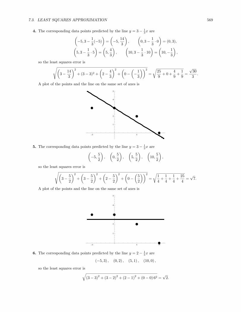
7.3. LEAST SQUARES APPROXIMATION 569
4. The corresponding data points predicted by the line y = 3− 13x are(
−5, 3− 1
3(−5)
)=
(−5,
14
3
),
(0, 3− 1
3· 0)
= (0, 3),(5, 3− 1
3· 5)
=
(5,
4
3
),
(10, 3− 1
3· 10
)=
(10,−1
3
),
so the least squares error is√(3− 14
3
)2
+ (3− 3)2 +
(2− 4
3
)2
+
(0−
(−1
3
))2
=
√25
9+ 0 +
4
9+
1
9=
√30
3.
A plot of the points and the line on the same set of axes is
-5 5 10
1
2
3
4
5
5. The corresponding data points predicted by the line y = 3− 13x are(
−5,5
2
),
(0,
5
2
),
(5,
5
2
),
(10,
5
2
),
so the least squares error is√(3− 5
2
)2
+
(3− 5
2
)2
+
(2− 5
2
)2
+
(0−
(5
2
))2
=
√1
4+
1
4+
1
4+
25
4=√
7.
A plot of the points and the line on the same set of axes is
-5 5 10
1
2
3
4
5
6. The corresponding data points predicted by the line y = 2− 15x are
(−5, 3) , (0, 2) , (5, 1) , (10, 0) ,
so the least squares error is√(3− 3)
2+ (3− 2)
2+ (2− 1)
2+ (0− 0) 62 =
√2.

570 CHAPTER 7. DISTANCE AND APPROXIMATION
A plot of the points and the line on the same set of axes is
-5 5 10
0.5
1.
1.5
2.
2.5
3.
7. We are looking for a line y = a+bx that best fits the given points. Using the least squares approximationtheorem, we want a solution to Ax = b, where
A =
1 x1
1 x2
......
1 xn
=
1 11 21 3
, x =
[ab
], b =
y1
y2
...yn
=
015
.Since
ATA =
[1 1 1
1 2 3
]1 1
1 2
1 3
=
[3 6
6 14
]⇒ (ATA)−1 =
[73 −1
−1 12
],
we get
x = (ATA)−1ATb =
[73 −1
−1 12
][1 1 1
1 2 3
]0
1
5
=
[−3
52
].
Thus the least squares approximation is y = −3 + 52x. To find the least squares error, compute
e = b−Ax =
0
1
5
−1 1
1 2
1 3
[−352
]=
12
−112
.Then ‖e‖ =
√(12
)2+ (−1)2 +
(12
)2=√
62 .
8. We are looking for a line y = a+bx that best fits the given points. Using the least squares approximationtheorem, we want a solution to Ax = b, where
A =
1 x1
1 x2
......
1 xn
=
1 11 21 3
, x =
[ab
], b =
y1
y2
...yn
=
631
.Since
ATA =
[1 1 1
1 2 3
]1 1
1 2
1 3
=
[3 6
6 14
]⇒ (ATA)−1 =
[73 −1
−1 12
],

7.3. LEAST SQUARES APPROXIMATION 571
we get
x = (ATA)−1ATb =
[73 −1
−1 12
][1 1 1
1 2 3
]6
3
1
=
[253
− 52
].
Thus the least squares approximation is y = 253 −
52x. To find the least squares error, compute
e = b−Ax =
6
3
1
−1 1
1 2
1 3
[ 253
− 52
]=
16
− 1316
.Then ‖e‖ =
√(16
)2+(− 1
3
)2+(
16
)2=√
66 .
9. We are looking for a line y = a+bx that best fits the given points. Using the least squares approximationtheorem, we want a solution to Ax = b, where
A =
1 x1
1 x2
......
1 xn
=
1 01 11 2
, x =
[ab
], b =
y1
y2
...yn
=
410
.Since
ATA =
[1 1 1
0 1 2
]1 0
1 1
1 2
=
[3 3
3 5
]⇒ (ATA)−1 =
[56 − 1
2
− 12
12
],
we get
x = (ATA)−1ATb =
[56 − 1
2
− 12
12
][1 1 1
0 1 2
]4
1
0
=
[113
−2
].
Thus the least squares approximation is y = 113 − 2x. To find the least squares error, compute
e = b−Ax =
4
1
0
−1 0
1 1
1 2
[ 113
−2
]=
13
− 2313
.Then ‖e‖ =
√(13
)2+(− 2
3
)2+(
13
)2=√
63 .
10. We are looking for a line y = a+bx that best fits the given points. Using the least squares approximationtheorem, we want a solution to Ax = b, where
A =
1 x1
1 x2
......
1 xn
=
1 01 11 2
, x =
[ab
], b =
y1
y2
...yn
=
335
.Since
ATA =
[1 1 1
0 1 2
]1 0
1 1
1 2
=
[3 3
3 5
]⇒ (ATA)−1 =
[56 − 1
2
− 12
12
],
572 CHAPTER 7. DISTANCE AND APPROXIMATION
we get
x = (ATA)−1ATb =
[56 − 1
2
− 12
12
][1 1 1
0 1 2
]3
3
5
=
[83
1
].
Thus the least squares approximation is y = 83 + x. To find the least squares error, compute
e = b−Ax =
3
3
5
−1 0
1 1
1 2
[ 83
1
]=
13
− 2313
.Then ‖e‖ =
√(13
)2+(− 2
3
)2+(
13
)2=√
63 .
11. We are looking for a line y = a+bx that best fits the given points. Using the least squares approximationtheorem, we want a solution to Ax = b, where
A =
1 x1
1 x2
......
1 xn
=
1 −51 01 51 10
, x =
[ab
], b =
y1
y2
...yn
=
−1
124
.Since
ATA =
[1 1 1 1
−5 0 5 10
]1 −5
1 0
1 5
1 10
=
[4 10
10 150
]⇒ (ATA)−1 =
[310 − 1
50
− 150
1125
],
we get
x = (ATA)−1ATb =
[310 − 1
50
− 150
1125
][1 1 1 1
−5 0 5 10
]−1
1
2
4
=
[710825
].
Thus the least squares approximation is y = 710 + 8
25x. To find the least squares error, compute
e = b−Ax =
−1
1
2
4
−
1 −5
1 0
1 5
1 10
[
710825
]=
− 1
10310
− 310110
.
Then ‖e‖ =
√(− 1
10
)2+(
310
)2+(− 3
10
)2+(
110
)2=√
55 .
12. We are looking for a line y = a+bx that best fits the given points. Using the least squares approximationtheorem, we want a solution to Ax = b, where
A =
1 x1
1 x2
......
1 xn
=
1 −51 01 51 10
, x =
[ab
], b =
y1
y2
...yn
=
3320
.Since
ATA =
[1 1 1 1
−5 0 5 10
]1 −5
1 0
1 5
1 10
=
[4 10
10 150
]⇒ (ATA)−1 =
[310 − 1
50
− 150
1125
],

7.3. LEAST SQUARES APPROXIMATION 573
we get
x = (ATA)−1ATb =
[310 − 1
50
− 150
1125
][1 1 1 1
−5 0 5 10
]3
3
2
0
=
[52
− 15
].
Thus the least squares approximation is y = 52 −
15x. To find the least squares error, compute
e = b−Ax =
3
3
2
0
−
1 −5
1 0
1 5
1 10
[
52
− 15
]=
− 1
21212
− 12
.Then ‖e‖ =
√(− 1
2
)2+(
12
)2+(
12
)2+(
12
)2= 1.
13. We are looking for a line y = a+bx that best fits the given points. Using the least squares approximationtheorem, we want a solution to Ax = b, where
A =
1 x1
1 x2
......
1 xn
=
1 11 21 31 41 5
, x =
[ab
], b =
y1
y2
...yn
=
13457
.Since
ATA =
[1 1 1 1 1
1 2 3 4 5
]
1 1
1 2
1 3
1 4
1 5
=
[5 15
15 55
]⇒ (ATA)−1 =
[1110 − 3
10
− 310
110
],
we get
x = (ATA)−1ATb =
[1110 − 3
10
− 310
110
][1 1 1 1 1
1 2 3 4 5
]
1
3
4
5
7
=
[− 1
575
].
Thus the least squares approximation is y = − 15 + 7
5x. To find the least squares error, compute
e = b−Ax =
1
3
4
5
7
−
1 1
1 2
1 3
1 4
1 5
[− 1
575
]=
− 1
525
0
− 2515
.
Then ‖e‖ =
√(− 1
5
)2+(
25
)2+ 02 +
(− 2
5
)2+(
15
)2=√
105 .
14. We are looking for a line y = a+bx that best fits the given points. Using the least squares approximationtheorem, we want a solution to Ax = b, where
A =
1 x1
1 x2
......
1 xn
=
1 11 21 31 41 5
, x =
[ab
], b =
y1
y2
...yn
=
108530
.

574 CHAPTER 7. DISTANCE AND APPROXIMATION
Since
ATA =
[1 1 1 1 1
1 2 3 4 5
]
1 1
1 2
1 3
1 4
1 5
=
[5 15
15 55
]⇒ (ATA)−1 =
[1110 − 3
10
− 310
110
],
we get
x = (ATA)−1ATb =
[1110 − 3
10
− 310
110
][1 1 1 1 1
1 2 3 4 5
]
10
8
5
3
0
=
[12710
− 52
].
Thus the least squares approximation is y = 12710 −
52x. To find the least squares error, compute
e = b−Ax =
10
8
5
3
0
−
1 1
1 2
1 3
1 4
1 5
[
12710
− 52
]=
− 1
5310
− 15310
− 15
.
Then ‖e‖ =
√(− 1
5
)2+(
310
)2+(− 1
5
)2+(
310
)2+(− 1
5
)2=√
3010 .
15. Following the method of Example 7.28, we substitute the given values of x into the quadratic equationa+ bx+ cx2 = y to get
a+ b+ c = 1
a+ 2b+ 4c = −2
a+ 3b+ 9c = 3
a+ 4b+ 16c = 4,
which in matrix form is 1 1 11 2 41 3 91 4 16
abc
=
1−2
34
.Thus we want the least squares approximation to Ax = b, where A is the 4× 3 matrix on the left andb is the matrix on the right in the above equation. Since
ATA =
1 1 1 1
1 2 3 4
1 4 9 16
1 1 1
1 2 4
1 3 9
1 4 16
=
4 10 30
10 30 100
30 100 354
⇒ (ATA)−1 =
314 − 27
454
− 274
12920 − 5
454 − 5
414
,we get
x = (ATA)−1ATb =
314 − 27
454
− 274
12920 − 5
454 − 5
414
1 1 1 1
1 2 3 4
1 4 9 16
1
−2
3
4
=
3
− 185
1
.Thus the least squares approximation is y = 3− 18
5 x+ x2.
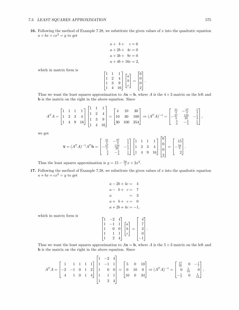
7.3. LEAST SQUARES APPROXIMATION 575
16. Following the method of Example 7.28, we substitute the given values of x into the quadratic equationa+ bx+ cx2 = y to get
a+ b+ c = 6
a+ 2b+ 4c = 0
a+ 3b+ 9c = 0
a+ 4b+ 16c = 2,
which in matrix form is 1 1 11 2 41 3 91 4 16
abc
=
6002
.Thus we want the least squares approximation to Ax = b, where A is the 4× 3 matrix on the left andb is the matrix on the right in the above equation. Since
ATA =
1 1 1 1
1 2 3 4
1 4 9 16
1 1 1
1 2 4
1 3 9
1 4 16
=
4 10 30
10 30 100
30 100 354
⇒ (ATA)−1 =
314 − 27
454
− 274
12920 − 5
454 − 5
414
,we get
x = (ATA)−1ATb =
314 − 27
454
− 274
12920 − 5
454 − 5
414
1 1 1 1
1 2 3 4
1 4 9 16
6
0
0
2
=
15
− 565
2
.Thus the least squares approximation is y = 15− 56
5 x+ 2x2.
17. Following the method of Example 7.28, we substitute the given values of x into the quadratic equationa+ bx+ cx2 = y to get
a− 2b+ 4c = 4
a− b+ c = 7
a = 3
a+ b+ c = 0
a+ 2b+ 4c = −1,
which in matrix form is 1 −2 41 −1 11 0 01 1 11 2 4
abc
=
4730−1
.Thus we want the least squares approximation to Ax = b, where A is the 5× 3 matrix on the left andb is the matrix on the right in the above equation. Since
ATA =
1 1 1 1 1
−2 −1 0 1 2
4 1 0 1 4
1 −2 4
1 −1 1
1 0 0
1 1 1
1 2 4
=
5 0 10
0 10 0
10 0 34
⇒ (ATA)−1 =
1735 0 − 1
7
0 110 0
− 17 0 1
14
,

576 CHAPTER 7. DISTANCE AND APPROXIMATION
we get
x = (ATA)−1ATb =
1735 0 − 1
7
0 110 0
− 17 0 1
14
1 1 1 1 1
−2 −1 0 1 2
4 1 0 1 4
4
7
3
0
−1
=
185
− 1710
− 12
.
Thus the least squares approximation is y = 185 −
1710x−
12x
2.
18. Following the method of Example 7.28, we substitute the given values of x into the quadratic equationa+ bx+ cx2 = y to get
a− 2b+ 4c = 0
a− b+ c = −11
a = −10
a+ b+ c = −9
a+ 2b+ 4c = 8,
which in matrix form is 1 −2 41 −1 11 0 01 1 11 2 4
abc
=
0
−11−10−9
8
.Thus we want the least squares approximation to Ax = b, where A is the 5× 3 matrix on the left andb is the matrix on the right in the above equation. Since
ATA =
1 1 1 1 1
−2 −1 0 1 2
4 1 0 1 4
1 −2 4
1 −1 1
1 0 0
1 1 1
1 2 4
=
5 0 10
0 10 0
10 0 34
⇒ (ATA)−1 =
1735 0 − 1
7
0 110 0
− 17 0 1
14
,
we get
x = (ATA)−1ATb =
1735 0 − 1
7
0 110 0
− 17 0 1
14
1 1 1 1 1
−2 −1 0 1 2
4 1 0 1 4
0
−11
−10
−9
8
=
−62595
4
.
Thus the least squares approximation is y = − 625 + 9
5x+ 4x2.
19. The normal equation is ATAx = ATb. We have
ATA =
[3 1 11 1 2
]3 11 11 2
=
[11 66 6
]
ATb =
[1 3 2−2 −2 1
]111
=
[54
],
so that the normal form of this system is [11 66 6
]x =
[54
].

7.3. LEAST SQUARES APPROXIMATION 577
Thus
x =
[11 6
6 6
]−1 [5
4
]=
[15 − 1
5
− 15
1130
][5
4
]=
[15715
]is the least squares solution.
20. The normal equation is ATAx = ATb. We have
ATA =
[1 3 2−2 −2 1
]1 −23 −22 1
=
[14 −6−6 9
]
ATb =
[1 3 2−2 −2 1
]111
=
[6−3
],
so that the normal form of this system is[14 −6−6 9
]x =
[6−3
].
Thus
x =
[14 −6
−6 9
]−1 [6
−3
]=
[110
115
115
745
][6
−3
]=
[215
− 115
]is the least squares solution.
21. The normal equation is ATAx = ATb. We have
ATA =
[1 0 2 3−2 −3 5 0
]1 −20 −32 53 0
=
[14 88 38
]
ATb =
[1 0 2 3−2 −3 5 0
]41−2
4
=
[12−21
],
so that the normal form of this system is[14 88 38
]x =
[12−21
].
Thus
x =
[14 8
8 38
]−1 [12
−21
]=
[19234 − 2
117
− 2117
7234
][12
−21
]=
[43
− 56
]is the least squares solution.
22. The normal equation is ATAx = ATb. We have
ATA =
[1 2 −1 00 −1 1 2
]1 02 −1−1 1
0 2
=
[6 −3−3 6
]
ATb =
[1 2 −1 00 −1 1 2
]15−1
2
=
[12−2
],

578 CHAPTER 7. DISTANCE AND APPROXIMATION
so that the normal form of this system is[6 −3−3 6
]x =
[12−2
].
Thus
x =
[6 −3
−3 6
]−1 [12
−2
]=
[29
19
19
29
][12
−2
]=
[22989
]is the least squares solution.
23. Instead of trying to invert ATA, we instead use an alternative method, row-reducing[ATA ATb
].
We will see that ATA does not reduce to the identity matrix, so that the system does not have a uniquesolution. We get
ATA =
1 1 0 11 0 −1 −10 1 1 10 1 1 0
1 1 0 01 0 1 10 −1 1 11 −1 1 0
=
3 0 2 10 3 −2 −12 −2 3 21 −1 2 2
ATb =
1 1 0 11 0 −1 −10 1 1 10 1 1 0
1−3
24
=
2−5
3−1
.Row-reducing, we have
3 0 2 1 20 3 −2 −1 −52 −2 3 2 31 −1 2 2 −1
→
1 0 0 −1 40 1 0 1 −50 0 1 2 −50 0 0 0 0
.So ATA is not invertible, and therefore there is not a unique solution. The general solution is
4 + t−5− t−5− 2t
t
=
4−5−5
0
+ t
1−1−2
1
.24. Instead of trying to invert ATA, we instead use an alternative method, row-reducing
[ATA ATb
].
We will see that ATA does not reduce to the identity matrix, so that the system does not have a uniquesolution. We get
ATA =
0 1 1 11 −1 0 11 1 1 10 −1 0 1
0 1 1 01 −1 1 −11 0 1 01 1 1 1
=
3 0 3 00 3 1 23 1 4 00 2 0 2
ATb =
0 1 1 11 −1 0 11 1 1 10 −1 0 1
53−1
1
=
338−2
.Row-reducing, we have
3 0 3 0 30 3 1 2 33 1 4 0 80 2 0 2 −2
→
1 0 0 1 −50 1 0 1 −10 0 1 −1 60 0 0 0 0
.

7.3. LEAST SQUARES APPROXIMATION 579
So ATA is not invertible, and therefore there is not a unique solution. The general solution is−5− t−1− t6 + tt
=
−5−1
60
+ t
−1−1
11
.25. Solving these equations corresponds to solving Ax = b where
A =
1 1 −10 −1 23 2 −1−1 0 1
b =
26110
.To solve, we row-reduce
[ATA ATb
]:
ATA =
1 0 3 −11 −1 2 0−1 2 −1 1
1 1 −10 −1 23 2 −1−1 0 1
=
11 7 −57 6 −5−5 −5 7
ATb =
1 0 3 −11 −1 2 0−1 2 −1 1
26110
=
3518−1
.Row-reducing, we have 11 7 −5 35
7 6 −5 18
−5 −5 7 −1
→1 0 0 42
11
0 1 0 1911
0 0 1 4211
.Thus the best approximation is
x =
xyz
=
421119114211
.26. Solving these equations corresponds to solving Ax = b where
A =
2 3 11 1 1−1 1 −1
0 2 1
b =
217140
.To solve, we row-reduce
[ATA ATb
]:
ATA =
2 1 −1 03 1 1 21 1 −1 1
2 3 11 1 1−1 1 −1
0 2 1
=
6 6 46 15 54 5 4
ATb =
2 1 −1 03 1 1 21 1 −1 1
217140
=
358414
.Row-reducing, we have 6 6 4 35
6 15 5 84
4 5 4 14
→1 0 0 469
66
0 1 0 22433
0 0 1 − 13311
.

580 CHAPTER 7. DISTANCE AND APPROXIMATION
Thus the best approximation is
x =
xyz
=
4696622433
− 13311
.27. With Ax = QRx = b, we get
Rx = QTb, or
[3 1
0 1
]x =
[23
23
13
13 − 2
323
] 2
3
−1
=
[3
−2
].
Back-substitution gives the solution
x =
[53
−2
].
28. With Ax = QRx = b, we get
Rx = QTb, or
[√6 −
√6
2
0 1√2
]x =
[1√6
2√6− 1√
61√2
0 1√2
]1
1
1
=
[2√6√2
].
Back-substitution gives the solution
x =
[43
2
].
29. We are looking for a line y = a+bx that best fits the given points. Using the least squares approximationtheorem, we want a solution to Ax = b, where
A =
1 x1
1 x2
......
1 xn
=
1 201 401 481 601 801 100
, x =
[ab
], b =
y1
y2
...yn
=
14.53136
45.559
73.5
.
Since
ATA =
[1 1 1 1 1 1
20 40 48 60 80 100
]
1 20
1 40
1 48
1 60
1 80
1 100
=
[6 348
348 24304
]⇒ (ATA)−1 =
[15191545 − 29
2060
− 292060
14120
],
we get
x = (ATA)−1ATb =
[15191545 − 29
2060
− 292060
14120
][1 1 1 1 1 1
20 40 48 60 80 100
]
14.5
31
36
45.5
59
73.5
=
[0.918
0.730
].
Thus the least squares approximation is y = 0.918 + 0.730x.

7.3. LEAST SQUARES APPROXIMATION 581
30. (a) We are looking for a line L = a + bF that best fits the given points. Using the least squaresapproximation theorem, we want a solution to Ax = b, where
A =
1 x1
1 x2
......
1 xn
=
1 21 41 61 8
, x =
[ab
], b =
y1
y2
...yn
=
7.49.611.513.6
.Since
ATA =
[1 1 1 1
2 4 6 8
]1 2
1 4
1 6
1 8
=
[4 20
20 120
]⇒ (ATA)−1 =
[32 − 1
4
− 14
120
],
we get
x = (ATA)−1ATb =
[32 − 1
4
− 14
120
][1 1 1 1
2 4 6 8
]7.4
9.6
11.5
13.6
=
[5.4
1.025
].
Thus the least squares approximation is L = 5.4 + 1.025F . a = 5.4 represents the length of thespring when no force is applied (F = 0).
(b) When a weight of 5 ounces is attached, the spring length will be about 5.4 + 1.025 · 5 = 10.525inches.
31. (a) We are looking for a line y = a+ bx that best fits the given points. Letting x = 0 correspond to1920 and using the least squares approximation theorem, we want a solution to Ax = b, where
A =
1 x1
1 x2
......
1 xn
=
1 01 101 201 301 401 501 601 70
, x =
[ab
], b =
y1
y2
...yn
=
54.159.762.968.269.770.873.775.4
.
Since
ATA =
[8 280
280 14000
]⇒ (ATA)−1 =
[512 − 1
120
− 1120
14200
],
we get
x = (ATA)−1ATb =
[512 − 1
120
− 1120
14200
][1 1 1 1 1 1 1 1
0 10 20 30 40 50 60 70
]
54.1
59.7
62.9
68.2
69.7
70.8
73.7
75.4
=
[56.63
0.291
].
Thus the least squares approximation is y = 56.63 + 0.291x. The model predicts that the lifeexpectancy of someone born in 2000 is y(80) = 56.63 + 0.291 · 80 = 79.91 years.

582 CHAPTER 7. DISTANCE AND APPROXIMATION
(b) To see how good the model is, compute the least squares error:
e = b−Ax =
54.159.762.968.269.770.873.775.4
−
1 01 101 201 301 401 501 601 70
[56.630.291
]=
−2.530.160.452.841.43−0.38−0.39−1.6
, so ‖e‖ ≈ 4.43.
The model is not bad, with an error of under 10% of the initial value.
32. (a) Following the method of Example 7.28, we substitute the given values of x into the equationa+ bx+ cx2 = y to get
a+ 0.5b+ 0.25c = 11
a+ b+ c = 17
a+ 1.5b+ 2.25c = 21
a+ 2b+ 4c = 23
a+ 3b+ 9c = 18,
which in matrix form is 1 0.5 0.251 1 11 1.5 2.251 2 41 3 9
abc
=
1117212318
.Thus we want the least squares approximation to Ax = b, where A is the 5× 3 matrix on the leftand b is the matrix on the right in the above equation. Since
ATA =
1 1 1 1 10.5 1 1.5 2 30.25 1 2.25 4 9
1 0.5 0.251 1 11 1.5 2.251 2 41 3 9
=
5 8 16.58 16.5 39.5
16.5 39.5 103.125
⇒
(ATA)−1 =
3.330 −4.082 1.031−4.082 5.735 −1.543
1.031 −1.543 0.436
,we get
x = (ATA)−1ATb =
3.330 −4.082 1.031−4.082 5.735 −1.543
1.031 −1.543 0.436
1 1 1 1 10.5 1 1.5 2 30.25 1 2.25 4 9
1117212318
=
1.91820.306−4.972
.
Thus the least squares approximation is y = 1.918 + 20.306t− 4.972t2.
(b) The height at which the object was released is y(0) ≈ 1.918 m. Its initial velocity was y′(0) ≈20.306 m/sec, and its acceleration due to gravity is y′′(t) ≈ −9.944 m/s
2.
(c) The object hits the ground when y(t) = 0. Solving the quadratic using the quadratic formulagives y ≈ −0.092 and y ≈ 4.176 seconds. So the object hits the ground after about 4.176 seconds.
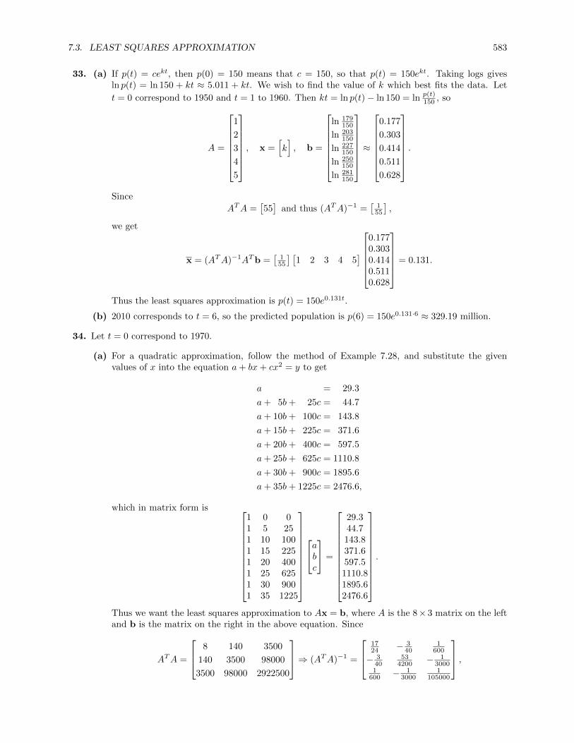
7.3. LEAST SQUARES APPROXIMATION 583
33. (a) If p(t) = cekt, then p(0) = 150 means that c = 150, so that p(t) = 150ekt. Taking logs givesln p(t) = ln 150 + kt ≈ 5.011 + kt. We wish to find the value of k which best fits the data. Let
t = 0 correspond to 1950 and t = 1 to 1960. Then kt = ln p(t)− ln 150 = ln p(t)150 , so
A =
1
2
3
4
5
, x =[k], b =
ln 179
150
ln 203150
ln 227150
ln 250150
ln 281150
≈
0.177
0.303
0.414
0.511
0.628
.
Since
ATA =[55]
and thus (ATA)−1 =[
155
],
we get
x = (ATA)−1ATb =[
155
] [1 2 3 4 5
]
0.1770.3030.4140.5110.628
= 0.131.
Thus the least squares approximation is p(t) = 150e0.131t.
(b) 2010 corresponds to t = 6, so the predicted population is p(6) = 150e0.131·6 ≈ 329.19 million.
34. Let t = 0 correspond to 1970.
(a) For a quadratic approximation, follow the method of Example 7.28, and substitute the givenvalues of x into the equation a+ bx+ cx2 = y to get
a = 29.3
a+ 5b+ 25c = 44.7
a+ 10b+ 100c = 143.8
a+ 15b+ 225c = 371.6
a+ 20b+ 400c = 597.5
a+ 25b+ 625c = 1110.8
a+ 30b+ 900c = 1895.6
a+ 35b+ 1225c = 2476.6,
which in matrix form is
1 0 01 5 251 10 1001 15 2251 20 4001 25 6251 30 9001 35 1225
abc
=
29.344.7143.8371.6597.51110.81895.62476.6
.
Thus we want the least squares approximation to Ax = b, where A is the 8× 3 matrix on the leftand b is the matrix on the right in the above equation. Since
ATA =
8 140 3500
140 3500 98000
3500 98000 2922500
⇒ (ATA)−1 =
1724 − 3
401
600
− 340
534200 − 1
30001
600 − 13000
1105000
,
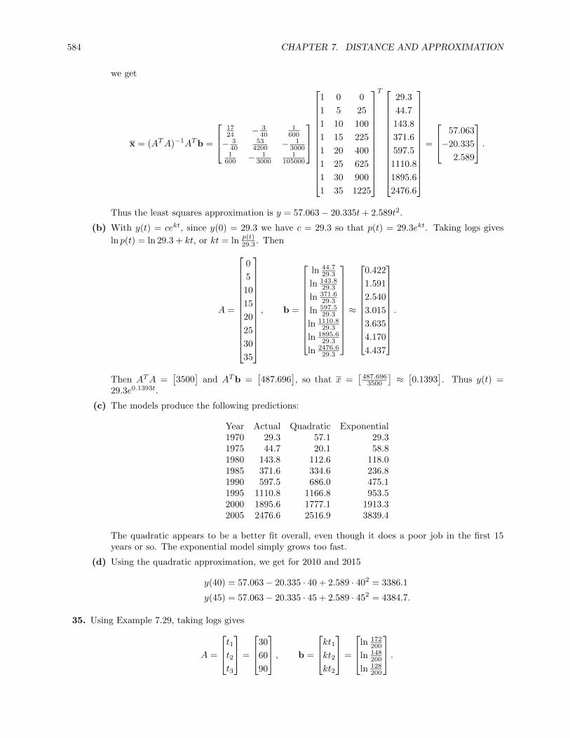
584 CHAPTER 7. DISTANCE AND APPROXIMATION
we get
x = (ATA)−1ATb =
1724 − 3
401
600
− 340
534200 − 1
30001
600 − 13000
1105000
1 0 0
1 5 25
1 10 100
1 15 225
1 20 400
1 25 625
1 30 900
1 35 1225
T
29.3
44.7
143.8
371.6
597.5
1110.8
1895.6
2476.6
=
57.063
−20.335
2.589
.
Thus the least squares approximation is y = 57.063− 20.335t+ 2.589t2.
(b) With y(t) = cekt, since y(0) = 29.3 we have c = 29.3 so that p(t) = 29.3ekt. Taking logs gives
ln p(t) = ln 29.3 + kt, or kt = ln p(t)29.3 . Then
A =
0
5
10
15
20
25
30
35
, b =
ln 44.729.3
ln 143.829.3
ln 371.629.3
ln 597.529.3
ln 1110.829.3
ln 1895.629.3
ln 2476.629.3
≈
0.422
1.591
2.540
3.015
3.635
4.170
4.437
.
Then ATA =[3500
]and ATb =
[487.696
], so that x =
[487.696
3500
]≈[0.1393
]. Thus y(t) =
29.3e0.1393t.
(c) The models produce the following predictions:
Year Actual Quadratic Exponential1970 29.3 57.1 29.31975 44.7 20.1 58.81980 143.8 112.6 118.01985 371.6 334.6 236.81990 597.5 686.0 475.11995 1110.8 1166.8 953.52000 1895.6 1777.1 1913.32005 2476.6 2516.9 3839.4
The quadratic appears to be a better fit overall, even though it does a poor job in the first 15years or so. The exponential model simply grows too fast.
(d) Using the quadratic approximation, we get for 2010 and 2015
y(40) = 57.063− 20.335 · 40 + 2.589 · 402 = 3386.1
y(45) = 57.063− 20.335 · 45 + 2.589 · 452 = 4384.7.
35. Using Example 7.29, taking logs gives
A =
t1t2t3
=
30
60
90
, b =
kt1kt2
kt2
=
ln 172200
ln 148200
ln 128200
.

7.3. LEAST SQUARES APPROXIMATION 585
Then ATA =[12600
]and ATb ≈
[−62.8
], so that x ≈
[− 62.8
12600
]≈ −0.005. Thus k = −0.005 and
p(t) = ce−0.005t. To compute the half-life, we want to solve 12c = ce−0.005t, so that −0.005t = ln 1
2 =
− ln 2; then t = ln 20.005 ≈ 139 days.
36. We want to find the best fit z = a+ bx+ cy to the given data; the data give the equations
a − 4c = 0
a+ 5b = 0
a+ 4b− c = 1
a+ b− 3c = 1
a− b− 5c = −2,
which in matrix form is 1 0 −41 5 01 4 −11 1 −31 −1 −5
abc
=
0011−2
.Thus we want the least squares approximation to Ax = b, where A is the 5× 3 matrix on the left andb is the matrix on the right in the above equation. Since
ATA =
5 9 −13
9 43 −2
−13 −2 51
⇒ (ATA)−1 =
218915 − 433
1554115
− 43315
8615 − 107
1554115 − 107
1513415
,we get
x = (ATA)−1ATb =
218915 − 433
1554115
− 43315
8615 − 107
1554115 − 107
1513415
1 1 1 1 1
0 5 4 1 −1
−4 0 −1 −3 −5
0
0
1
1
−2
=
433
− 83
113
.
Thus the least squares approximation is y = 13 (43− 8x+ 11y).
37. We have
A =
[11
]⇒ AT =
[1 1
]⇒ ATA =
[2], (ATA)−1 =
[12
].
So the standard matrix of the orthogonal projection onto W is
P = A(ATA)−1AT =
[1
1
] [12
] [1 1
]=
[12
12
12
12
].
Then
projW (v) = Pv =
[12
12
12
12
][3
4
]=
[7272
].
38. We have
A =
[1−2
]⇒ AT =
[1 −2
]⇒ ATA =
[5], (ATA)−1 =
[15
].
So the standard matrix of the orthogonal projection onto W is
P = A(ATA)−1AT =
[1
−2
] [15
] [1 −2
]=
[15 − 2
5
− 25
45
].

586 CHAPTER 7. DISTANCE AND APPROXIMATION
Then
projW (v) = Pv =
[15 − 2
5
− 25
45
][1
1
]=
[− 1
525
].
39. We have
A =
111
⇒ AT =[1 1 1
]⇒ ATA =
[3], (ATA)−1 =
[13
].
So the standard matrix of the orthogonal projection onto W is
P = A(ATA)−1AT =
1
1
1
[ 13
] [1 1 1
]=
13
13
13
13
13
13
13
13
13
.Then
projW (v) = Pv =
13
13
13
13
13
13
13
13
13
1
2
3
=
2
2
2
.40. We have
A =
22−1
⇒ AT =[2 2 −1
]⇒ ATA =
[9], (ATA)−1 =
[19
].
So the standard matrix of the orthogonal projection onto W is
P = A(ATA)−1AT =
2
2
−1
[ 19
] [2 2 −1
]=
49
49 − 2
949
49 − 2
9
− 29 − 2
919
.Then
projW (v) = Pv =
49
49 − 2
949
49 − 2
9
− 29 − 2
919
1
0
0
=
4949
− 29
.41. We have
A =
1 10 1−1 1
⇒ AT =
[1 0 −11 1 1
]⇒ ATA =
[2 00 3
], (ATA)−1 =
[12 00 1
3
].
So the standard matrix of the orthogonal projection onto W is
P = A(ATA)−1AT =
1 1
0 1
−1 1
[ 12 0
0 13
][1 0 −1
1 1 1
]=
56
13 − 1
613
13
13
− 16
13
56
.Then
projW (v) = Pv =
56
13 − 1
613
13
13
− 16
13
56
1
0
0
=
5613
− 16
.
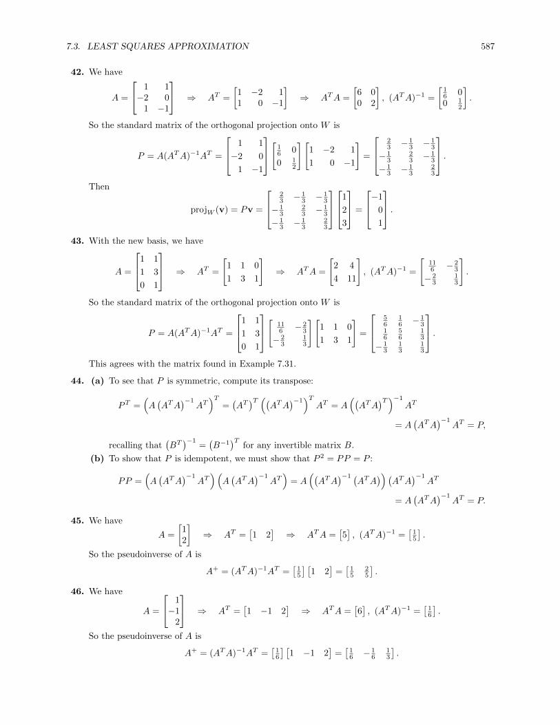
7.3. LEAST SQUARES APPROXIMATION 587
42. We have
A =
1 1−2 0
1 −1
⇒ AT =
[1 −2 11 0 −1
]⇒ ATA =
[6 00 2
], (ATA)−1 =
[16 00 1
2
].
So the standard matrix of the orthogonal projection onto W is
P = A(ATA)−1AT =
1 1
−2 0
1 −1
[ 16 0
0 12
][1 −2 1
1 0 −1
]=
23 − 1
3 − 13
− 13
23 − 1
3
− 13 − 1
323
.Then
projW (v) = Pv =
23 − 1
3 − 13
− 13
23 − 1
3
− 13 − 1
323
1
2
3
=
−1
0
1
.43. With the new basis, we have
A =
1 1
1 3
0 1
⇒ AT =
[1 1 0
1 3 1
]⇒ ATA =
[2 4
4 11
], (ATA)−1 =
[116 − 2
3
− 23
13
].
So the standard matrix of the orthogonal projection onto W is
P = A(ATA)−1AT =
1 1
1 3
0 1
[ 116 − 2
3
− 23
13
][1 1 0
1 3 1
]=
56
16 − 1
316
56
13
− 13
13
13
.This agrees with the matrix found in Example 7.31.
44. (a) To see that P is symmetric, compute its transpose:
PT =(A(ATA
)−1AT)T
=(AT)T ((
ATA)−1)T
AT = A((ATA
)T)−1
AT
= A(ATA
)−1AT = P,
recalling that(BT)−1
=(B−1
)Tfor any invertible matrix B.
(b) To show that P is idempotent, we must show that P 2 = PP = P :
PP =(A(ATA
)−1AT)(
A(ATA
)−1AT)
= A((ATA
)−1 (ATA
)) (ATA
)−1AT
= A(ATA
)−1AT = P.
45. We have
A =
[12
]⇒ AT =
[1 2
]⇒ ATA =
[5], (ATA)−1 =
[15
].
So the pseudoinverse of A is
A+ = (ATA)−1AT =[
15
] [1 2
]=[
15
25
].
46. We have
A =
1−1
2
⇒ AT =[1 −1 2
]⇒ ATA =
[6], (ATA)−1 =
[16
].
So the pseudoinverse of A is
A+ = (ATA)−1AT =[
16
] [1 −1 2
]=[
16 − 1
613
].

588 CHAPTER 7. DISTANCE AND APPROXIMATION
47. We have
A =
1 3
−1 1
0 2
⇒ AT =
[1 −1 0
3 1 2
]⇒ ATA =
[2 2
2 14
], (ATA)−1 =
[712 − 1
12
− 112
112
].
So the pseudoinverse of A is
A+ = (ATA)−1AT =
[712 − 1
12
− 112
112
][1 −1 0
3 1 2
]=
[13 − 2
3 − 16
16
16
16
].
48. We have
A =
1 3
3 1
2 2
⇒ AT =
[1 3 2
3 1 2
]⇒ ATA =
[14 10
10 14
], (ATA)−1 =
[748 − 5
48
− 548
748
].
So the pseudoinverse of A is
A+ = (ATA)−1AT =
[748 − 5
48
− 548
748
][1 3 2
3 1 2
]=
[− 1
613
112
13 − 1
6112
].
49. We have
A =
[1 10 1
]⇒ AT =
[1 01 1
]⇒ ATA =
[1 11 2
], (ATA)−1 =
[2 −1−1 1
].
So the pseudoinverse of A is
A+ = (ATA)−1AT =
[2 −1−1 1
] [1 01 1
]=
[1 −10 1
].
Note that this is the inverse A−1 of A.
50. We have
A =
[1 2
3 4
]⇒ AT =
[1 3
2 4
]⇒ ATA =
[10 14
14 20
], (ATA)−1 =
[5 − 7
2
− 72
52
].
So the pseudoinverse of A is
A+ = (ATA)−1AT =
[5 − 7
2
− 72
52
][1 3
2 4
]=
[−2 1
32 − 1
2
].
Note that this is the inverse A−1 of A.
51. We have
A =
1 0 0
1 0 1
0 1 1
1 1 1
⇒ AT =
1 1 0 1
0 0 1 1
0 1 1 1
⇒ ATA =
3 1 2
1 2 2
2 2 3
, (ATA)−1 =
23
13 − 2
313
53 − 4
3
− 23 − 4
353
.So the pseudoinverse of A is
A+ = (ATA)−1AT =
23
13 − 2
313
53 − 4
3
− 23 − 4
353
1 1 0 1
0 0 1 1
0 1 1 1
=
23 0 − 1
313
13 −1 1
323
− 23 1 1
3 − 13
.

7.3. LEAST SQUARES APPROXIMATION 589
52. We have
A =
1 2 00 1 −11 1 −20 0 2
⇒ AT =
1 0 1 02 1 1 00 −1 −2 2
,so that
ATA =
2 3 −2
3 6 −3
−2 −3 9
, (ATA)−1 =
157 −1 1
7
−1 23 0
17 0 1
7
.So the pseudoinverse of A is
A+ = (ATA)−1AT =
157 −1 1
7
−1 23 0
17 0 1
7
1 0 1 0
2 1 1 0
0 −1 −2 2
=
17 − 8
767
27
13
23 − 1
3 017 − 1
7 − 17
27
.53. (a) Since A is square with linearly independent columns, it is invertible, so that
A+ =(ATA
)−1AT = A−1
(AT)−1
AT = A−1.
(b) Let the columns of A be qi; then qi · qj = 0 if i 6= j and 1 if i = j. Then
ATA =
qT1...qTn
[q1 · · · qn]
= In,
so that A+ =(ATA
)−1AT = InA
T = AT . (Note that this makes sense, for if A were square, itwould be an orthogonal matrix and then part (a) would hold and AT = A−1.)
54. A+AA+ =((ATA
)−1AT)AA+ =
(ATA
)−1 (ATA
)A+ = A+.
55. We have A+A =(ATA
)−1ATA =
(ATA
)−1 (ATA
)= I, which is certainly a symmetric matrix.
56. (a) (cA)+ =(cAT cA
)−1cAT = 1
c2
(ATA
)−1cAT = 1
c
(ATA
)−1AT = 1
cAT .
(b) By Exercise 53(a), if A is square, then A+ = A−1. Also A−1 is square with linearly independent
columns, so that(A−1
)+=(A−1
)−1= A. Then(A+)
+=(A−1
)+= A.
(c) Since A is square, Exercise 53(a) applies to both A and AT , so that(AT)+
=(AT)−1
=(A−1
)T=(A+)T.
57. The fact that not all the points lie on the same vertical line means that there is at least one pair i, jsuch that xi 6= xj . Constructing the matrix A gives
A =
1 x1
......
1 xi...
...1 xj...
...1 xn
.
Since xi 6= xj , the columns are not multiples of one another, so must be linearly independent. Sincethe columns of A are linearly independent, the points have a unique least squares approximating line,by part (b) of the Least Squares Theorem.

590 CHAPTER 7. DISTANCE AND APPROXIMATION
58. Constructing the matrix A gives
A =
1 x1 x21 · · · xk1
......
.... . .
...1 xn x2
n · · · xkn
.The solution(s) to Ax = b are the least squares approximating polynomials of degree k; by the LeastSquares Theorem, there is a unique solution when the columns of A are linearly independent. Nowsuppose that
a0a1 + a1a2 + · · ·+ akak+1 = 0.
This means that a0 + a1xi + · · ·+ akxki = 0 for all i. But since at least k+ 1 of the xi are distinct, the
polynomial a0 + a1x+ · · ·+ akxk has at least k+ 1 distinct roots, so it must be the zero polynomial by
Exercise 62 in Section 6.2. Thus all of the ai are zero, so the columns of A are linearly independent.
7.4 The Singular Value Decomposition
1. We have
ATA =
[2 00 3
] [2 00 3
]=
[4 00 9
].
Then the singular values of A are the square roots of the eigenvalues of this matrix which, since thematrix is diagonal, are 4 and 9. Thus the singular values of A are σ1 =
√9 = 3 and σ2 =
√4 = 2.
2. We have
ATA =
[2 11 2
] [2 11 2
]=
[5 44 5
].
Then the singular values of A are the square roots of the eigenvalues of this matrix.
det(ATA− λI) =
∣∣∣∣5− λ 44 5− λ
∣∣∣∣ = (5− λ)2 − 16 = λ2 − 10λ+ 9 = (λ− 9)(λ− 1),
so that the eigenvalues are 9 and 1. Thus the singular values of A are σ1 =√
9 = 3 and σ2 =√
1 = 1.
3. We have
ATA =
[1 01 0
] [1 10 0
]=
[1 11 1
].
Then the singular values of A are the square roots of the eigenvalues of this matrix.
det(ATA− λI) =
∣∣∣∣1− λ 11 1− λ
∣∣∣∣ = (1− λ)2 − 1 = λ2 − 2λ = λ(λ− 2),
so that the singular values of A are σ1 =√
2 and σ2 =√
0 = 0.
4. We have
ATA =
[√2 0
1√
2
] [√2 1
0√
2
]=
[2√
2√2 3
].
Then the singular values of A are the square roots of the eigenvalues of this matrix.
det(ATA− λI) =
∣∣∣∣2− λ √2√
2 3− λ
∣∣∣∣ = (2− λ)(3− λ)− 2 = λ2 − 5λ+ 4 = (λ− 4)(λ− 1),
so that the singular values of A are σ1 =√
4 = 2 and σ2 =√
1 = 1.
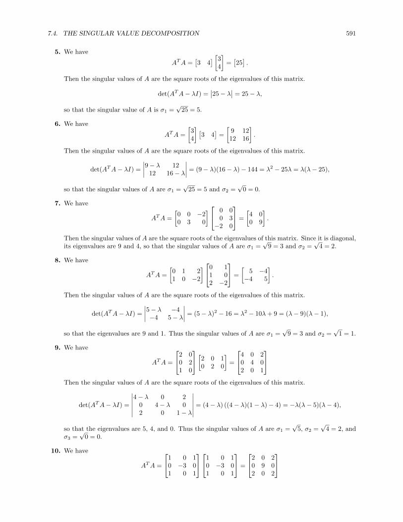
7.4. THE SINGULAR VALUE DECOMPOSITION 591
5. We have
ATA =[3 4
] [34
]=[25].
Then the singular values of A are the square roots of the eigenvalues of this matrix.
det(ATA− λI) =∣∣25− λ
∣∣ = 25− λ,
so that the singular value of A is σ1 =√
25 = 5.
6. We have
ATA =
[34
] [3 4
]=
[9 1212 16
].
Then the singular values of A are the square roots of the eigenvalues of this matrix.
det(ATA− λI) =
∣∣∣∣9− λ 1212 16− λ
∣∣∣∣ = (9− λ)(16− λ)− 144 = λ2 − 25λ = λ(λ− 25),
so that the singular values of A are σ1 =√
25 = 5 and σ2 =√
0 = 0.
7. We have
ATA =
[0 0 −20 3 0
] 0 00 3−2 0
=
[4 00 9
].
Then the singular values of A are the square roots of the eigenvalues of this matrix. Since it is diagonal,its eigenvalues are 9 and 4, so that the singular values of A are σ1 =
√9 = 3 and σ2 =
√4 = 2.
8. We have
ATA =
[0 1 21 0 −2
]0 11 02 −2
=
[5 −4−4 5
].
Then the singular values of A are the square roots of the eigenvalues of this matrix.
det(ATA− λI) =
∣∣∣∣5− λ −4−4 5− λ
∣∣∣∣ = (5− λ)2 − 16 = λ2 − 10λ+ 9 = (λ− 9)(λ− 1),
so that the eigenvalues are 9 and 1. Thus the singular values of A are σ1 =√
9 = 3 and σ2 =√
1 = 1.
9. We have
ATA =
2 00 21 0
[2 0 10 2 0
]=
4 0 20 4 02 0 1
Then the singular values of A are the square roots of the eigenvalues of this matrix.
det(ATA− λI) =
∣∣∣∣∣∣4− λ 0 2
0 4− λ 02 0 1− λ
∣∣∣∣∣∣ = (4− λ) ((4− λ)(1− λ)− 4) = −λ(λ− 5)(λ− 4),
so that the eigenvalues are 5, 4, and 0. Thus the singular values of A are σ1 =√
5, σ2 =√
4 = 2, andσ3 =
√0 = 0.
10. We have
ATA =
1 0 10 −3 01 0 1
1 0 10 −3 01 0 1
=
2 0 20 9 02 0 2

592 CHAPTER 7. DISTANCE AND APPROXIMATION
Then the singular values of A are the square roots of the eigenvalues of this matrix.
det(ATA− λI) =
∣∣∣∣∣∣2− λ 0 2
0 9− λ 02 0 2− λ
∣∣∣∣∣∣ = (9− λ)((2− λ)2 − 4
)= −(λ− 9)(λ− 4)λ
so that the eigenvalues are 9, 4, and 0. Thus the singular values of A are σ1 =√
9 = 3, σ2 =√
4 = 2,and σ3 =
√0 = 0.
11. From Exercise 3,
ATA =
[1 11 1
],
with eigenvalues 2 and 0, so that the singular values of A are σ1 =√
2 and σ2 =√
0 = 0. To find thecorresponding eigenspaces, row-reduce:
[ATA− 2I 0
]=
[−1 1 0
1 −1 0
]→[1 −1 00 0 0
]⇒ x1 =
[11
][ATA− 0I 0
]=
[1 1 01 1 0
]→[1 1 00 0 0
]⇒ x2 =
[1−1
].
These vectors are already orthogonal since they correspond to distinct eigenvalues. Normalizing eachof them gives
v1 =
[1√2
1√2
], v2 =
[1√2
− 1√2
], so that V =
[v1 v2
]=
[1√2
1√2
1√2− 1√
2
].
The first column of the matrix U is
u1 =1
σ1Av1 =
1√2
[1 1
0 0
][1√2
1√2
]=
[1
0
].
We do not use v2 since it corresponds to an eigenvalue of zero. We must extend this to an orthonormalbasis of R2 by adjoining a second vector, u2, to get an orthogonal matrix. Clearly e2 is such a vector.Thus
A = UΣV T =
[1 0
0 1
][√2 0
0 0
][1√2
1√2
1√2− 1√
2
]is a singular value decomposition of A.
12. We have
ATA =
[1 11 1
] [1 11 1
]=
[2 22 2
].
The characteristic polynomial of ATA is
det(ATA− λI) =
∣∣∣∣2− λ 22 2− λ
∣∣∣∣ = (2− λ)2 − 4 = λ2 − 4λ = λ(λ− 4).
Thus the eigenvalues are λ1 = 4 and λ2 = 0 (and so the singular values are σ1 = 2 and σ2 = 0). Tofind the corresponding eigenspaces, row-reduce:
[ATA− 4I 0
]=
[−2 2 0
2 −2 0
]→[1 −1 00 0 0
]⇒ x1 =
[11
][ATA− 0I 0
]=
[2 2 02 2 0
]→[1 1 00 0 0
]⇒ x2 =
[1−1
].

7.4. THE SINGULAR VALUE DECOMPOSITION 593
To find the matrix V , we must normalize each of these vectors (they are already orthogonal since theycorrespond to distinct eigenvalues). This gives
v1 =
[1√2
1√2
], v2 =
[1√2
− 1√2
], so that V =
[v1 v2
]=
[1√2
1√2
1√2− 1√
2
].
The first column of the matrix U is
u1 =1
σ1Av1 =
1
2
[1 1
1 1
][1√2
1√2
]=
[1√2
1√2
].
We do not use v2 since it corresponds to an eigenvalue of zero. We must extend this to an orthonormalbasis of R2 by adjoining a second vector, u2, to get an orthogonal matrix. By looking at the matrix
V , we see that such a vector is
[1√2
− 1√2
]. Thus
A = UΣV T =
[1√2
1√2
1√2− 1√
2
][2 0
0 0
][1√2
1√2
1√2− 1√
2
]
is a singular value decomposition of A.
13. We have
ATA =
[0 −3−2 0
] [0 −2−3 0
]=
[9 00 4
].
This matrix is diagonal, so its eigenvalues are its diagonal entries, which are λ1 = 9 and λ2 = 4.Therefore the singular values of A are σ1 =
√9 = 3 and σ2 =
√4 = 2. To find the corresponding
eigenspaces, row-reduce:
[ATA− 9I 0
]=
[0 0 00 −5 0
]→[0 1 00 0 0
]⇒ x1 =
[10
][ATA− 4I 0
]=
[4 0 00 0 0
]→[1 0 00 0 0
]⇒ x2 =
[01
].
These vectors are already orthonormal, so we set
v1 = x1, v2 = x2, so that V =[v1 v2
]=
[1 00 1
].
Then U is found by
u1 =1
σ1Av1 =
1
3
[0 −2
−3 0
][1
0
]=
[0
−1
]
u2 =1
σ2Av2 =
1
2
[0 −2
−3 0
][0
1
]=
[−1
0
].
Thus
A = UΣV T =
[0 −1−1 0
] [3 00 2
] [1 00 1
]is a singular value decomposition of A.

594 CHAPTER 7. DISTANCE AND APPROXIMATION
14. We have
ATA =
[1 1−1 1
] [1 −11 1
]=
[2 00 2
].
This matrix is diagonal, so its eigenvalues are its diagonal entries. So the only eigenvalue is 2 and thesingular values of A are σ1 = σ2 =
√2. To find the corresponding eigenspace, row-reduce:
[ATA− 2I 0
]=
[0 0 00 0 0
]⇒ x1 =
[10
], x2 =
[01
].
These vectors are already orthonormal, so we set
v1 = x1, v2 = x2, so that V =[v1 v2
]=
[1 00 1
].
Then U is found by
u1 =1
σ1Av1 =
1√2
[1 −1
1 1
][1
0
]=
[1√2
1√2
]
u2 =1
σ2Av2 =
1√2
[1 −1
1 1
][0
1
]=
[− 1√
21√2
].
Thus
A = UΣV T =
[1√2− 1√
21√2
1√2
][√2 0
0√
2
][1 0
0 1
]is a singular value decomposition of A.
15. From Exercise 5,
ATA =[25],
so that the only eigenvalue is 25 and therefore the only singular value is σ1 =√
25 = 5. To find thecorresponding eigenspace, row-reduce:[
ATA− 25I 0]
=[0 0
]⇒ x1 =
[1].
This single vector forms an orthonormal set; let v1 = x1, so that
V =[v1
]=[1].
Then U is found by
u1 =1
σ1Av1 =
1
5
[3
4
] [1]
=
[3545
].
We extend this to an orthonormal basis for R2 by adjoining the orthogonal unit vector
[− 4
535
]. Since
Σ should be 2× 1 and there is only one singular value, we adjoin a zero to the singular value. Thus
A = UΣV T =
[35 − 4
545
35
][5
0
] [1]
is a singular value decomposition of A.

7.4. THE SINGULAR VALUE DECOMPOSITION 595
16. From Exercise 6,
ATA =
[9 1212 16
],
with eigenvalues 25 and 0, so that the singular values of A are σ1 =√
25 = 5 and σ2 =√
0 = 0. Tofind the corresponding eigenspaces, row-reduce:
[ATA− 25I 0
]=
[−16 12 0
12 −9 0
]→[1 − 3
4 00 0 0
]⇒ x1 =
[34
][ATA− 0I 0
]=
[9 12 0
12 16 0
]→[1 4
3 00 0 0
]⇒ x2 =
[−4
3
].
To find the matrix V , we must normalize each of these vectors (they are already orthogonal since theycorrespond to distinct eigenvalues). This gives
v1 =
[3545
], v2 =
[− 4
535
], so that V =
[v1 v2
]=
[35 − 4
545
35
].
The first column of the matrix U is
u1 =1
σ1Av1 =
1
5
[3 4
] [ 3545
]=[1].
Then U is the 1 × 1 matrix containing 1 as its entry. Since Σ should be 1 × 2 and there is only onenonzero singular value, we adjoin a zero to the singular value, so that
A = UΣV T =[1] [
5 0] [ 3
545
− 45
35
]
is a singular value decomposition of A.
17. From Exercise 7,
ATA =
[4 00 9
],
with eigenvalues 9 and 4, so with singular values 3 and 2. To find the corresponding eigenspaces,row-reduce: [
ATA− 9I 0]
=
[−5 0 0
0 0 0
]→[1 0 00 0 0
]⇒ x1 =
[01
][ATA− 4I 0
]=
[0 0 00 5 0
]→[0 1 00 0 0
]⇒ x2 =
[10
].
These vectors are already orthonormal, so we set
v1 = x1, v2 = x2, so that V =[v1 v2
]=
[0 11 0
].
Then U is found by
u1 =1
σ1Av1 =
1
3
0 00 3−2 0
[01
]=
010
u2 =
1
σ2Av2 =
1
2
0 00 3−2 0
[10
]=
00−1
.

596 CHAPTER 7. DISTANCE AND APPROXIMATION
We must extend u1 and u2 to an orthonormal basis for R3. Clearly u3 = e1 =
100
works. Then U is
the matrix whose columns are the ui. Now, Σ should be 3×2, so we add a row of zeros at the bottom,giving
A = UΣV T =
0 0 11 0 00 −1 0
3 00 20 0
[0 11 0
]for a singular value decomposition of A.
18. From Exercise 8,
ATA =
[5 −4−4 5
],
with eigenvalues 9 and 1 and singular values σ1 =√
9 = 3 and σ2 =√
1 = 1. To find the correspondingeigenspaces, row-reduce:[
ATA− 9I 0]
=
[−4 −4 0−4 −4 0
]→[1 1 00 0 0
]⇒ x1 =
[1−1
][ATA− I 0
]=
[4 −4 0−4 4 0
]→[1 −1 00 0 0
]⇒ x2 =
[11
].
These vectors are already orthogonal, but we must normalize them:
v1 =x1
‖x1‖=
[1√2
− 1√2
], v2 =
x2
‖x2‖=
[1√2
1√2
], so that V =
[v1 v2
]=
[1√2
1√2
− 1√2
1√2
]Then U is found by
u1 =1
σ1Av1 =
1
3
0 1
1 0
2 −2
[
1√2
− 1√2
]=
− 1
3√
21
3√
24
3√
2
u2 =1
σ2Av2 =
1
1
0 1
1 0
2 −2
[
1√2
1√2
]=
1√2
1√2
0
.We must extend u1 and u2 to an orthonormal basis for R3. To keep computations simpler, we multiplyu1 by 3
√2 and v1 by
√2. Then adjoin e1, e2, and e3 to these vectors and row-reduce:−1 1 1 0 0
1 1 0 1 0
4 0 0 0 1
→1 0 0 0 1
4
0 1 0 1 − 14
0 0 1 −1 12
.Then a basis for the column space, which is R3, is given by the columns of the original matrix corre-sponding to leading 1’s, which is u1, u2, and x3 = e1. Finally, we must turn this into an orthonormalbasis:
x′3 = x3−−1 · 1 + 1 · 0 + 4 · 0−1 · (−1) + 1 · 1 + 4 · 4
−1
1
4
− 1 · 1 + 1 · 0 + 0 · 01 · 1 + 1 · 1 + 0 · 0
1
1
0
=
1
0
0
+1
18
−1
1
4
− 1
2
1
1
0
=
49
− 4929
.Normalizing this vector gives
u3 =x′3‖x3‖
=
23
− 2313
.

7.4. THE SINGULAR VALUE DECOMPOSITION 597
Then U is the matrix whose columns are the ui. Now, Σ should be 3× 2, so we add a row of zeros atthe bottom, giving
A = UΣV T =
− 1
3√
21√2
23
13√
21√2− 2
3
43√
20 1
3
3 0
0 1
0 0
[
1√2− 1√
21√2
1√2
]
for a singular value decomposition of A.
19. From Exercise 9,
ATA =
4 0 20 4 02 0 1
,with eigenvalues 5, 4, and 0, so the singular values are σ1 =
√5, σ2 = 2, and σ3 = 0. To find the
corresponding eigenspaces, row-reduce:
[ATA− 5I 0
]=
−1 0 2 00 −1 0 02 0 −4 0
→1 0 −2 0
0 1 0 00 0 0 0
⇒ x1 =
201
[ATA− 4I 0
]=
0 0 2 00 0 0 02 0 −3 0
→1 0 0 0
0 0 1 00 0 0 0
⇒ x2 =
010
[ATA− 0I 0
]=
4 0 2 00 4 0 02 0 1 0
→1 0 1
2 00 1 0 00 0 0 0
⇒ x3 =
−102
.These vectors are already orthogonal, but we must normalize them:
v1 =x1
‖x1‖=
2√5
01√5
, v2 =x2
‖x2‖=
0
1
0
, v3 =x3
‖x3‖=
− 1√
5
02√5
,so that
V =[v1 v2 v3
]=
2√5
0 − 1√5
0 1 01√5
0 2√5
Then U is found by
u1 =1
σ1Av1 =
1√5
[2 0 1
0 2 0
]2√5
01√5
=
[1
0
]
u2 =1
σ2Av2 =
1
2
[2 0 1
0 2 0
]0
1
0
=
[0
1
].
We do not use v3 since it corresponds to a zero singular value. Then u1 and u2 already form a basisfor R2. Now, Σ should be 3× 2, so we add a column of zeros on the right, giving
A = UΣV T =
[1 0
0 1
][√5 0 0
0 2 0
]2√5
0 1√5
0 1 0
− 1√5
0 2√5
for a singular value decomposition of A.

598 CHAPTER 7. DISTANCE AND APPROXIMATION
20. We have
ATA =
1 11 11 1
[1 1 11 1 1
]=
2 2 22 2 22 2 2
Then the singular values of A are the square roots of the eigenvalues of this matrix.
det(ATA− λI) =
∣∣∣∣∣∣2− λ 2 2
2 2− λ 22 2 2− λ
∣∣∣∣∣∣ = −λ2(λ− 6),
so that the eigenvalues are 6 and 0. Thus the singular values of A are σ1 =√
6 and σ2 =√
0 = 0. Tofind the corresponding eigenspaces, row-reduce:
[ATA− 6I 0
]=
−4 2 2 02 −4 2 02 2 −4 0
→1 0 −1 0
0 1 −1 00 0 0 0
⇒ x1 =
111
[ATA− 0I 0
]=
2 2 2 02 2 2 02 2 2 0
→1 1 1 0
0 0 0 00 0 0 0
⇒ x2 =
1−1
0
, x3 =
10−1
.We must orthogonalize x2 and x3. Use Gram-Schmidt:
x′3 = x3 −x2 · x3
x2 · x2x2 =
1
0
−1
− 1
2
1
−1
0
=
1212
−1
Multiply through by 2 to clear fractions, giving
x′′3 =
11−2
.Finally, we normalize the vectors:
v1 =x1
‖x1‖=
1√3
1√3
1√3
, v2 =x2
‖x2‖=
1√2
0
− 1√2
, v3 =x′′3‖x′′3‖
=
1√6
1√6
− 2√6
⇒
V =[v1 v2 v3
]=
1√3
1√2
1√6
1√3
0 1√6
1√3− 1√
2− 2√
6
.Then U is found by
u1 =1
σ1Av1 =
1√6
[1 1 1
1 1 1
]1√3
1√3
1√3
=
[1√2
1√2
].
We do not use v2 or v3 since they correspond to a zero singular value. Then we extend u1 to an
orthonormal basis of R2 by adding the orthogonal unit vector u2 =
[− 1√
21√2
]. Finally, Σ must be 2× 3,
so we adjoin zeros as required:
A = UΣV T =
[1√2− 1√
21√2
1√2
][√6 0 0
0 0 0
]1√3
1√3
1√3
1√2
0 − 1√2
1√6
1√6− 2√
6
for a singular value decomposition of A.
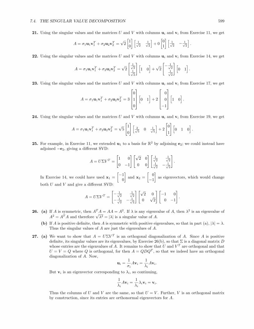
7.4. THE SINGULAR VALUE DECOMPOSITION 599
21. Using the singular values and the matrices U and V with columns ui and vi from Exercise 11, we get
A = σ1u1vT1 + σ2u2v
T2 =√
2
[10
] [1√2
1√2
]+ 0
[01
] [1√2− 1√
2
].
22. Using the singular values and the matrices U and V with columns ui and vi from Exercise 14, we get
A = σ1u1vT1 + σ2u2v
T2 =√
2
[1√2
1√2
] [1 0
]+√
2
[− 1√
21√2
] [0 1
].
23. Using the singular values and the matrices U and V with columns ui and vi from Exercise 17, we get
A = σ1u1vT1 + σ2u2v
T2 = 3
0
1
0
[0 1]
+ 2
0
0
−1
[1 0].
24. Using the singular values and the matrices U and V with columns ui and vi from Exercise 19, we get
A = σ1u1vT1 + σ2u2v
T2 =√
5
[1
0
] [2√5
0 1√5
]+ 2
[0
1
] [0 1 0
].
25. For example, in Exercise 11, we extended u1 to a basis for R2 by adjoining e2; we could instead haveadjoined −e2, giving a different SVD:
A = UΣV T =
[1 0
0 −1
][√2 0
0 0
][1√2
1√2
1√2− 1√
2
].
In Exercise 14, we could have used x1 =
[−1
0
]and x2 =
[0−1
]as eigenvectors, which would change
both U and V and give a different SVD:
A = UΣV T =
[− 1√
21√2
− 1√2− 1√
2
][√2 0
0√
2
][−1 0
0 −1
].
26. (a) If A is symmetric, then ATA = AA = A2. If λ is any eigenvalue of A, then λ2 is an eigenvalue of
A2 = ATA and therefore√λ2 = |λ| is a singular value of A.
(b) If A is positive definite, then A is symmetric with positive eigenvalues, so that in part (a), |λ| = λ.Thus the singular values of A are just the eigenvalues of A.
27. (a) We want to show that A = UΣV T is an orthogonal diagonalization of A. Since A is positivedefinite, its singular values are its eigenvalues, by Exercise 26(b), so that Σ is a diagonal matrix Dwhose entries are the eigenvalues of A. It remains to show that U and V T are orthogonal and thatU = V = Q where Q is orthogonal, for then A = QDQT , so that we indeed have an orthogonaldiagonalization of A. Now,
ui =1
σiAvi =
1
λiAvi.
But vi is an eigenvector corresponding to λi, so continuing,
1
λiAvi =
1
λiλivi = vi.
Thus the columns of U and V are the same, so that U = V . Further, V is an orthogonal matrixby construction, since its entries are orthonormal eigenvectors for A.
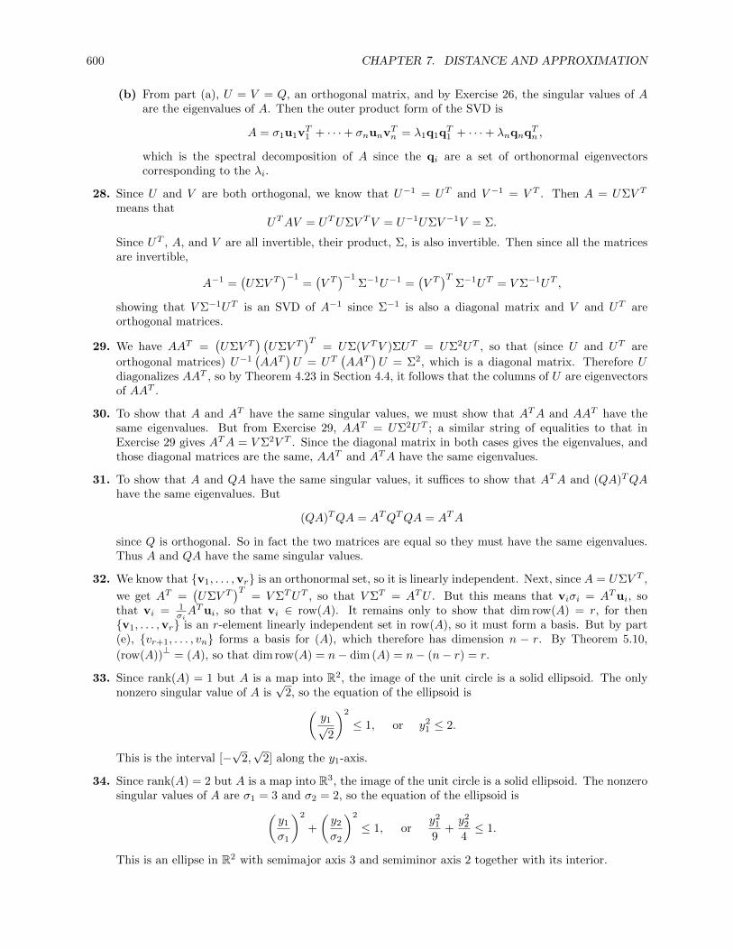
600 CHAPTER 7. DISTANCE AND APPROXIMATION
(b) From part (a), U = V = Q, an orthogonal matrix, and by Exercise 26, the singular values of Aare the eigenvalues of A. Then the outer product form of the SVD is
A = σ1u1vT1 + · · ·+ σnunv
Tn = λ1q1q
T1 + · · ·+ λnqnq
Tn ,
which is the spectral decomposition of A since the qi are a set of orthonormal eigenvectorscorresponding to the λi.
28. Since U and V are both orthogonal, we know that U−1 = UT and V −1 = V T . Then A = UΣV T
means thatUTAV = UTUΣV TV = U−1UΣV −1V = Σ.
Since UT , A, and V are all invertible, their product, Σ, is also invertible. Then since all the matricesare invertible,
A−1 =(UΣV T
)−1=(V T)−1
Σ−1U−1 =(V T)T
Σ−1UT = V Σ−1UT ,
showing that V Σ−1UT is an SVD of A−1 since Σ−1 is also a diagonal matrix and V and UT areorthogonal matrices.
29. We have AAT =(UΣV T
) (UΣV T
)T= UΣ(V TV )ΣUT = UΣ2UT , so that (since U and UT are
orthogonal matrices) U−1(AAT
)U = UT
(AAT
)U = Σ2, which is a diagonal matrix. Therefore U
diagonalizes AAT , so by Theorem 4.23 in Section 4.4, it follows that the columns of U are eigenvectorsof AAT .
30. To show that A and AT have the same singular values, we must show that ATA and AAT have thesame eigenvalues. But from Exercise 29, AAT = UΣ2UT ; a similar string of equalities to that inExercise 29 gives ATA = V Σ2V T . Since the diagonal matrix in both cases gives the eigenvalues, andthose diagonal matrices are the same, AAT and ATA have the same eigenvalues.
31. To show that A and QA have the same singular values, it suffices to show that ATA and (QA)TQAhave the same eigenvalues. But
(QA)TQA = ATQTQA = ATA
since Q is orthogonal. So in fact the two matrices are equal so they must have the same eigenvalues.Thus A and QA have the same singular values.
32. We know that {v1, . . . ,vr} is an orthonormal set, so it is linearly independent. Next, since A = UΣV T ,
we get AT =(UΣV T
)T= V ΣTUT , so that V ΣT = ATU . But this means that viσi = ATui, so
that vi = 1σiATui, so that vi ∈ row(A). It remains only to show that dim row(A) = r, for then
{v1, . . . ,vr} is an r-element linearly independent set in row(A), so it must form a basis. But by part(e), {vr+1, . . . , vn} forms a basis for (A), which therefore has dimension n − r. By Theorem 5.10,
(row(A))⊥
= (A), so that dim row(A) = n− dim (A) = n− (n− r) = r.
33. Since rank(A) = 1 but A is a map into R2, the image of the unit circle is a solid ellipsoid. The onlynonzero singular value of A is
√2, so the equation of the ellipsoid is(
y1√2
)2
≤ 1, or y21 ≤ 2.
This is the interval [−√
2,√
2] along the y1-axis.
34. Since rank(A) = 2 but A is a map into R3, the image of the unit circle is a solid ellipsoid. The nonzerosingular values of A are σ1 = 3 and σ2 = 2, so the equation of the ellipsoid is(
y1
σ1
)2
+
(y2
σ2
)2
≤ 1, ory2
1
9+y2
2
4≤ 1.
This is an ellipse in R2 with semimajor axis 3 and semiminor axis 2 together with its interior.

7.4. THE SINGULAR VALUE DECOMPOSITION 601
35. Since rank(A) = 2 and A is a map into R2, the image of the unit sphere is an ellipsoid. The nonzerosingular values of A are σ1 =
√5 and σ2 = 2, so the equation of the ellipsoid is(y1
σ1
)2
+
(y2
σ2
)2
= 1, ory2
1
5+y2
2
4= 1.
This is an ellipse in R2 with semimajor axis√
5 and semiminor axis 2.
36. Since rank(A) = 2 but A is a map into R3, the image of the unit sphere is a solid ellipsoid. The nonzerosingular values of A are σ1 = 3 and σ2 = 2, so the equation of the ellipsoid is(
y1
σ1
)2
+
(y2
σ2
)2
≤ 1, ory2
1
9+y2
2
4≤ 1.
This is an ellipse in R2 with semimajor axis 3 and semiminor axis 2 lying in the y1y2-plane, togetherwith its interior in that plane.
37. (a) From example 7.37, ‖A‖2 is the largest singular value,√
2. Thus ‖A‖2 =√
2.
(b) Since A is not invertible, cond2(A) =∞.
38. (a) From example 7.37, ‖A‖2 is the largest singular value, 3. Thus ‖A‖2 = 3.
(b) Since A is not invertible, cond2(A) =∞.
39. We first compute the singular values of A:
ATA =
[1 1
0.9 1
] [1 0.91 1
]=
[2 1.9
1.9 1.81
].
Then the characteristic polynomial for ATA is∣∣∣∣2− λ 1.91.9 1.81− λ
∣∣∣∣ = (2− λ)(1.81− λ)− 3.61 = λ2 − 3.81x+ 0.01.
Solving using a CAS gives λ1 ≈ 3.807 and λ2 ≈ 0.00263, so that the singular values are σ1 =√
3.807 ≈1.951 and σ2 =
√0.00263 ≈ 0.0512.
(a) From Example 7.37, ‖A‖2 = σ1 ≈ 1.95.
(b) cond2(A) = σ1
σ2≈ 38.1.
40. We first compute the singular values of A:
ATA =
10 10010 1000 1
[ 10 10 0100 100 1
]=
10100 10100 10010100 10100 100100 100 1
.Using technology, the characteristic polynomial is −λ3 + 20201λ2 − 200λ, with roots λ1 ≈ 20201,λ2 ≈ 0.0099, and λ3 = 0, so that the singular values are σ1 ≈ 142.13, σ2 ≈ 0.0995, and σ3 = 0.
(a) From Example 7.37, ‖A‖2 = σ1 ≈ 142.13.
(b) Since A is not invertible, cond2(A) =∞.
41. From Exercise 11,
A = UΣV T =
[1 0
0 1
][√2 0
0 0
][1√2
1√2
1√2− 1√
2
]is a singular value decomposition of the matrix A from Exercise 3. So
A+ = V Σ+UT =
[1√2
1√2
1√2− 1√
2
][1√2
0
0 0
][1 0
0 1
]=
[12 012 0
].
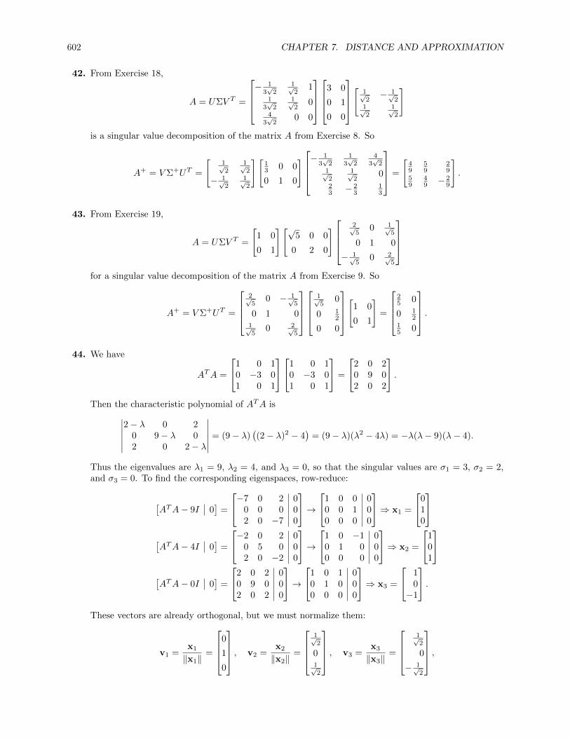
602 CHAPTER 7. DISTANCE AND APPROXIMATION
42. From Exercise 18,
A = UΣV T =
− 1
3√
21√2
11
3√
21√2
04
3√
20 0
3 0
0 1
0 0
[
1√2− 1√
21√2
1√2
]
is a singular value decomposition of the matrix A from Exercise 8. So
A+ = V Σ+UT =
[1√2
1√2
− 1√2
1√2
][13 0 0
0 1 0
]− 1
3√
21
3√
24
3√
21√2
1√2
023 − 2
313
=
[49
59
29
59
49 − 2
9
].
43. From Exercise 19,
A = UΣV T =
[1 0
0 1
][√5 0 0
0 2 0
]2√5
0 1√5
0 1 0
− 1√5
0 2√5
for a singular value decomposition of the matrix A from Exercise 9. So
A+ = V Σ+UT =
2√5
0 − 1√5
0 1 01√5
0 2√5
1√5
0
0 12
0 0
[
1 0
0 1
]=
25 0
0 12
15 0
.44. We have
ATA =
1 0 10 −3 01 0 1
1 0 10 −3 01 0 1
=
2 0 20 9 02 0 2
.Then the characteristic polynomial of ATA is∣∣∣∣∣∣
2− λ 0 20 9− λ 02 0 2− λ
∣∣∣∣∣∣ = (9− λ)((2− λ)2 − 4
)= (9− λ)(λ2 − 4λ) = −λ(λ− 9)(λ− 4).
Thus the eigenvalues are λ1 = 9, λ2 = 4, and λ3 = 0, so that the singular values are σ1 = 3, σ2 = 2,and σ3 = 0. To find the corresponding eigenspaces, row-reduce:
[ATA− 9I 0
]=
−7 0 2 00 0 0 02 0 −7 0
→1 0 0 0
0 0 1 00 0 0 0
⇒ x1 =
010
[ATA− 4I 0
]=
−2 0 2 00 5 0 02 0 −2 0
→1 0 −1 0
0 1 0 00 0 0 0
⇒ x2 =
101
[ATA− 0I 0
]=
2 0 2 00 9 0 02 0 2 0
→1 0 1 0
0 1 0 00 0 0 0
⇒ x3 =
10−1
.These vectors are already orthogonal, but we must normalize them:
v1 =x1
‖x1‖=
0
1
0
, v2 =x2
‖x2‖=
1√2
01√2
, v3 =x3
‖x3‖=
1√2
0
− 1√2
,

7.4. THE SINGULAR VALUE DECOMPOSITION 603
so that
V =[v1 v2 v3
]=
0 1√
21√2
1 0 0
0 1√2− 1√
2
.Then U is found by
u1 =1
σ1Av1 =
1
3
1 0 1
0 −3 0
1 0 1
0
1
0
=
0
−1
0
u2 =1
σ2Av2 =
1
2
1 0 1
0 −3 0
1 0 1
1√2
01√2
=
1√2
01√2
.We must extend u1 and u2 to an orthonormal basis for R3; clearly
u3 =
1√2
0
− 1√2
works. Then U is the matrix whose columns are the ui. Now, Σ should be 3 × 3, so we add zeros asappropriate, giving
A = UΣV T =
0 1√
21√2
−1 0 0
0 1√2− 1√
2
3 0 0
0 2 0
0 0 0
0 1 01√2
0 1√2
1√2
0 − 1√2
for a singular value decomposition of A. Then
A+ = V Σ+UT =
0 1√
21√2
1 0 0
0 1√2− 1√
2
13 0 0
0 12 0
0 0 0
0 −1 01√2
0 1√2
1√2
0 − 1√2
=
14 0 1
4
0 − 13 0
14 0 1
4
.45. We have
ATA =
[1 22 4
] [1 22 4
]=
[5 1010 20
].
Then the characteristic polynomial of ATA is∣∣∣∣5− λ 1010 20− λ
∣∣∣∣ = (5− λ)(20− λ)− 100 = λ2 − 25λ = λ(λ− 25).
Thus the eigenvalues are λ1 = 25 and λ2 = 0, so that the singular values are σ1 = 5 and σ2 = 0. Tofind the corresponding eigenspaces, row-reduce:
[ATA− 25I 0
]=
[−20 10 0
10 −5 0
]→[1 − 1
2 00 0 0
]⇒ x1 =
[12
][ATA− 0I 0
]=
[5 10 0
10 20 0
]→[1 2 00 0 0
]⇒ x2 =
[−2
1
].

604 CHAPTER 7. DISTANCE AND APPROXIMATION
These vectors are already orthogonal, but we must normalize them:
v1 =x1
‖x1‖=
[1√5
2√5
], v2 =
x2
‖x2‖=
[− 2√
51√5
], so that V =
[v1 v2
]=
[1√5− 2√
52√5
1√5
].
Then U is found by
u1 =1
σ1Av1 =
1
5
[1 2
2 4
][1√5
2√5
]=
[1√5
2√5
].
We must extend u1 to an orthonormal basis for R3; clearly
u2 =
[− 2√
51√5
]
works. Then U is the matrix whose columns are the ui. Now, Σ should be 2 × 2, so we add zeros asappropriate, giving
U =
[1√5− 2√
52√5
1√5
], Σ =
[5 0
0 0
], V =
[1√5− 2√
52√5
1√5
].
for a singular value decomposition of A. Then
A+ = V Σ+UT =
[1√5− 2√
52√5
1√5
][15 0
0 0
][1√5
2√5
− 2√5
1√5
]=
[125
225
225
425
],
so that
x = A+b =
[125
225
225
425
][3
5
]=
[13252625
].
46. We have
ATA =
3 00 00 2
[3 0 00 0 2
]=
9 0 00 0 00 0 4
.Since this matrix is diagonal, we can read off its eigenvalues, which are λ1 = 9, λ2 = 4, and λ3 = 0,so that the singular values are σ1 = 3, σ2 = 2 and σ3 = 0. To find the corresponding eigenspaces,row-reduce:
[ATA− 9I 0
]=
0 0 0 00 −9 0 00 0 −5 0
→0 1 0 0
0 0 1 00 0 0 0
⇒ x1 =
100
[ATA− 4I 0
]=
5 0 0 00 −4 0 00 0 0 0
→1 0 0 0
0 1 0 00 0 0 0
⇒ x2 =
001
[ATA− 0I 0
]=
9 0 0 00 0 0 00 0 4 0
→1 0 0 0
0 0 1 00 0 0 0
⇒ x3 =
010
.These vectors are already orthonormal, so setting vi = xi, we get
V =[v1 v2 v3
]=
1 0 00 0 10 1 0
.

7.4. THE SINGULAR VALUE DECOMPOSITION 605
Then U is found by
u1 =1
σ1Av1 =
1
3
[3 0 0
0 0 2
]1
0
0
=
[1
0
], u2 =
1
σ2Av2 =
1
2
[3 0 0
0 0 2
]0
0
1
=
[0
1
].
These vectors form an orthonormal basis for R2, so that U is the matrix whose columns are the ui.Now, Σ should be 2× 3, so we add a column of zeros on the right, giving
U =
[1 0
0 1
], Σ =
[3 0 0
0 2 0
], V =
1 0 0
0 0 1
0 1 0
for a singular value decomposition of A. Then
A+ = V Σ+UT =
1 0 0
0 0 1
0 1 0
13 0
0 12
0 0
[
1 0
0 1
]=
13 0
0 0
0 12
,so that
x = A+b =
13 0
0 0
0 12
[3
0
]=
1
0
0
.47. We have
ATA =
[1 1 11 1 1
]1 11 11 1
=
[3 33 3
].
The characteristic polynomial of ATA is∣∣∣∣3− λ 33 3− λ
∣∣∣∣ = (3− λ)2 − 9 = λ(λ− 6),
so that its eigenvalues are λ1 = 6 and λ2 = 0. Therefore the singular values of A are σ1 =√
6 andσ2 = 0. To find the corresponding eigenspaces, row-reduce:[
ATA− 6I 0]
=
[−3 3 0
3 −3 0
]→[1 −1 00 0 0
]⇒ x1 =
[11
][ATA− 0I 0
]=
[3 3 03 3 0
]→[1 1 00 0 0
]⇒ x2 =
[1−1
].
These vectors are already orthogonal, but we must normalize them:
v1 =x1
‖x1‖=
[1√2
1√2
], v2 =
x2
‖x2‖=
[1√2
− 1√2
],
so that
V =[v1 v2
]=
[1√2
1√2
1√2− 1√
2
].
Then U is found by
u1 =1
σ1Av1 =
1√6
1 1
1 1
1 1
[
1√2
1√2
]=
1√3
1√3
1√3
.
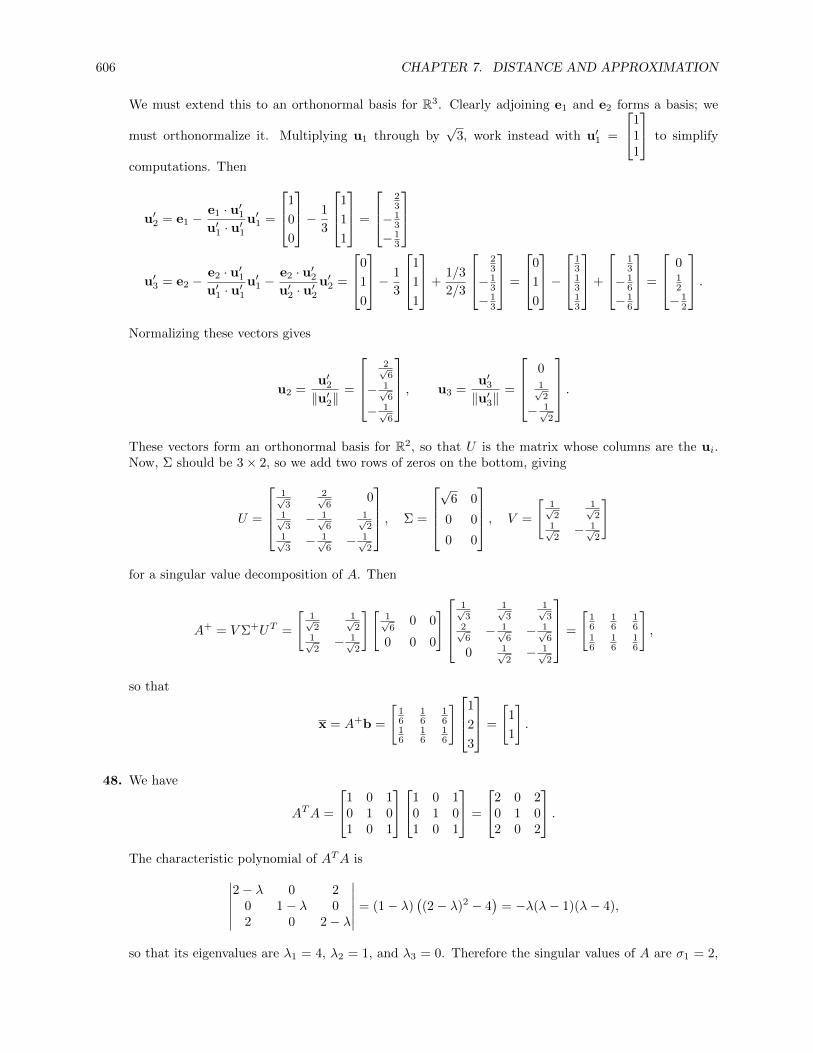
606 CHAPTER 7. DISTANCE AND APPROXIMATION
We must extend this to an orthonormal basis for R3. Clearly adjoining e1 and e2 forms a basis; we
must orthonormalize it. Multiplying u1 through by√
3, work instead with u′1 =
111
to simplify
computations. Then
u′2 = e1 −e1 · u′1u′1 · u′1
u′1 =
1
0
0
− 1
3
1
1
1
=
23
− 13
− 13
u′3 = e2 −
e2 · u′1u′1 · u′1
u′1 −e2 · u′2u′2 · u′2
u′2 =
0
1
0
− 1
3
1
1
1
+1/3
2/3
23
− 13
− 13
=
0
1
0
−
131313
+
13
− 16
− 16
=
012
− 12
.Normalizing these vectors gives
u2 =u′2‖u′2‖
=
2√6
− 1√6
− 1√6
, u3 =u′3‖u′3‖
=
01√2
− 1√2
.These vectors form an orthonormal basis for R2, so that U is the matrix whose columns are the ui.Now, Σ should be 3× 2, so we add two rows of zeros on the bottom, giving
U =
1√3
2√6
01√3− 1√
61√2
1√3− 1√
6− 1√
2
, Σ =
√
6 0
0 0
0 0
, V =
[1√2
1√2
1√2− 1√
2
]
for a singular value decomposition of A. Then
A+ = V Σ+UT =
[1√2
1√2
1√2− 1√
2
][1√6
0 0
0 0 0
]1√3
1√3
1√3
2√6− 1√
6− 1√
6
0 1√2− 1√
2
=
[16
16
16
16
16
16
],
so that
x = A+b =
[16
16
16
16
16
16
]1
2
3
=
[1
1
].
48. We have
ATA =
1 0 10 1 01 0 1
1 0 10 1 01 0 1
=
2 0 20 1 02 0 2
.The characteristic polynomial of ATA is∣∣∣∣∣∣
2− λ 0 20 1− λ 02 0 2− λ
∣∣∣∣∣∣ = (1− λ)((2− λ)2 − 4
)= −λ(λ− 1)(λ− 4),
so that its eigenvalues are λ1 = 4, λ2 = 1, and λ3 = 0. Therefore the singular values of A are σ1 = 2,

7.4. THE SINGULAR VALUE DECOMPOSITION 607
σ2 = 1 and σ3 = 0. To find the corresponding eigenspaces, row-reduce:
[ATA− 4I 0
]=
−2 0 2 00 −3 0 02 0 −2 0
→1 0 −1 0
0 1 0 00 0 0 0
⇒ x1 =
101
[ATA− 1I 0
]=
1 0 2 00 0 0 02 0 1 0
→1 0 0 0
0 0 1 00 0 0 0
⇒ x2 =
010
[ATA− 0I 0
]=
2 0 2 00 1 0 02 0 2 0
→1 0 1 0
0 1 0 00 0 0 0
⇒ x3 =
10−1
.These vectors are already orthogonal, but we must normalize them:
v1 =x1
‖x1‖=
1√2
01√2
, v2 =x2
‖x2‖=
0
1
0
, v3 =x3
‖x3‖=
1√2
0
− 1√2
,so that
V =[v1 v2 v3
]=
1√2
0 1√2
0 1 01√2
0 − 1√2
.Then U is found by
u1 =1
σ1Av1 =
1
2
1 0 1
0 1 0
1 0 1
1√2
01√2
=
1√2
01√2
, u2 =1
σ2Av2 =
1
1
1 0 1
0 1 0
1 0 1
0
1
0
=
0
1
0
We must extend this to an orthonormal basis for R3; clearly adjoining
u3 =
1√2
0
− 1√2
does the trick. Then U is the matrix whose columns are the ui. Now, Σ should be 3 × 3, so we addzeros as appropriate, giving
U =
1√2
0 1√2
0 1 01√2
0 − 1√2
, Σ =
2 0 0
0 1 0
0 0 0
, V =
1√2
0 1√2
0 1 01√2
0 − 1√2
for a singular value decomposition of A. Then
A+ = V Σ+UT =
1√2
0 1√2
0 1 01√2
0 − 1√2
12 0 0
0 1 0
0 0 0
1√2
0 1√2
0 1 01√2
0 − 1√2
=
14 0 1
4
0 1 014 0 1
4
,so that
x = A+b =
14 0 1
4
0 1 014 0 1
4
1
1
1
=
12
112
.

608 CHAPTER 7. DISTANCE AND APPROXIMATION
49. (a) The normal equation is ATAx = ATb. Now,
ATA =
[1 11 1
] [1 11 1
]=
[2 22 2
]ATb =
[1 11 1
] [01
]=
[11
].
Row-reducing, we get [ATA ATb
]=
[2 2 12 2 1
]→[1 1 1
20 0 0
].
Therefore x =
[120
], which satisfies x+ y = 1
2 .
(b) Letting y = t, the general solution is
x =
[12
0
]+
[−tt
]=
[12 − tt
].
The length of this solution vector is√(1
2− t)2
+ t2 =
√1
4− t+ 2t2.
(c) To minimize this length, it suffices to minimize 14 − t+ 2t2. This is an upward-opening parabola,
so its minimum occurs at t = − b2a = 1
4 . So the x of minimum length is[12 −
14
14
]=
[1414
],
as found in Example 7.40.
50. The definition of pseudoinverse in Section 7.3 is A+ =(ATA
)−1AT ; we must show that this is the
same as V Σ+UT , where UΣV T is an SVD for A. Now, AT =(UΣV T
)T= V ΣTUT = V ΣUT , and
ATA =(V ΣUT
) (UΣV T
)= V Σ2V T ,
since Σ is diagonal, thus symmetric, and U is orthogonal. Since A has linearly independent columns,the rank of A is the number of columns, so by Theorem 7.15, A has r nonzero singular values, so ATAhas only nonzero eigenvalues. Thus ATA is invertible, and(
ATA)−1
=(V Σ2V T
)−1=(V T)−1 (
Σ2)−1
V −1 = V(Σ−1
)2V T .
So finally,(ATA
)−1AT =
(V(Σ−1
)2V T) (V ΣUT
)= V
(Σ−1
)2 (V TV
)ΣUT = V Σ−1UT = V Σ+UT ,
which is the definition of A+ in this section. Note that since Σ is invertible, Exercise 28 tells us thatΣ−1 = Σ+.
51. Let A = UΣV T be an SVD for A. Suppose that
Σ =
[Dr×r OO O
]where D is an invertible diagonal matrix. Then
Σ+Σ =
[Ir×r OO O
]

7.4. THE SINGULAR VALUE DECOMPOSITION 609
since the nonzero entries of Σ are the inverses of the nonzero entries of Σ. Therefore
ΣΣ+Σ = Σ(Σ+Σ
)=
[Dr×r OO O
] [Ir×r OO O
]= Σ.
Similarly
Σ+ΣΣ+ =(Σ+Σ
)Σ+ =
[Ir×r OO O
] [D−1r×r OO O
]= Σ+.
(a) Just compute the product:
AA+A =(UΣV T
) (V Σ+UT
) (UΣV T
)= UΣ
(V TV
)Σ+(UTU
)ΣV T = UΣΣ+ΣV T
= UΣV T = A.
(b) Just compute the product:
A+AA+ =(V Σ+UT
) (UΣV T
) (V Σ+UT
)= V Σ+
(UTU
)Σ(V TV
)Σ+UT
= V Σ+ΣΣ+UT = V Σ+UT = A+.
(c) Compute the transpose of AA+:(AA+
)T=(AV Σ+UT
)T= U
(Σ+)TV TAT = U
(Σ+)T (
V TV)
ΣTUT
= U(Σ+)T
ΣTUT = U(ΣΣ+
)TUT .
But ΣΣ+ is a block matrix with the identity in the upper left and zeros elsewhere, so it issymmetric, and this expression becomes
U(ΣΣ+
)TUT = UΣΣ+UT =
(UΣV T
) (V Σ+UT
)= AA+,
so that AA+ is symmetric. A similar argument shows that A+A is symmetric.
52. As suggested in the hint, suppose that A′ is a matrix satisfying the Penrose conditions for A. Thenusing the fact that A+ and A′ each satisfy the Penrose conditions for A, we have
A′ = A′AA′ (Condition (b) for A′)
= A′(AA+A
)A′ (Condition (a) for A+)
= A′(AA+
)(AA′)
= A′(A+)TAT (A′)
TAT (Condition (c) for A′ and A+)
= A′(A+)T
(AA′A)T
= A′(A+)TAT (Condition (a) for A′)
= A′AA+ (Condition (c) for A+).
Similarly,
A+ = A+AA+ (Condition (b) for A+)
= A+ (AA′A)A+ (Condition (a) for A′)
=(A+A
)(A′A)A+
= AT(A+)TAT (A′)
TA+ (Condition (c) for A′ and A+)
=(AA+A
)T(A′)
TA+
= AT (A′)TA+ (Condition (a) for A+)
= A′ATA+ (Condition (c) for A′).
Since A′ and A+ are equal to the same thing, they are equal to each other.

610 CHAPTER 7. DISTANCE AND APPROXIMATION
53. Since A+AA+ = A+, the matrix A satisfies Penrose condition (a) for A+. Similarly, since AA+A = A,
the matrix A satisfies Penrose condition (b) for A+. Finally, since (A+A)T
= A+A, the matrix A
satisfies the first of the Penrose conditions in (c) for A+; similarly, since (AA+)T
= AA+, the matrixA satisfies the second of the Penrose conditions in (c) for A+. Since A satisfies all of the Penrose
conditions for A+, and since by Exercise 52 (A+)+
is the only matrix satisfying those conditions for
A+, we must have A = (A+)+
.
54. As in Exercise 53, we show that (A+)T
satisfies the Penrose conditions for AT ; then uniqueness tells
us that (A+)T
=(AT)+
.
(a) AT (A+)TAT = (AA+A)
T= AT .
(b) (A+)TAT (A+)
T= (A+AA+)
T= (A+)
T.
(c) We must show that both AT (A+)T
and (A+)TAT are symmetric:(
AT(A+)T)T
=((A+)T)T (
AT)T
= A+A =(A+A
)T= AT
(A+)T
((A+)TAT)T
=(AT)T ((
A+)T)T
= AA+ =(AA+
)T=(A+)TAT .
So (A+)T
=(AT)+
.
55. We show that A satisfies the Penrose conditions for A; then uniqueness tells us that A+ = A.
(a), (b) AAA = A2A = AA = A2 = A since A is idempotent.
(c) We must show that AA is symmetric. But AA = A2 = A, which is symmetric.
So A satisfies all three Penrose conditions and thus A+ = A.
56. It suffices to show that A+QT satisfies the Penrose conditions for QA. Using the fact that Q isorthogonal,
(a) (QA)(A+QT
)(QA) = Q (AA+)
(QTQ
)A = Q (AA+A) = QA.
(b)(A+QT
)(QA)
(A+QT
)= A+
(QTQ
)AA+QT = (A+AA+)QT = A+QT .
(c) We must show that both (QA)(A+QT
)and
(A+QT
)(QA) are symmetric:(
(QA)(A+QT
))T=(QT)T (
A+)TATQT = Q
(AA+
)TQT = Q
(AA+
)QT = (QA)
(A+QT
)((A+QT
)(QA)
)T= ATQT
(QT)T (
A+)T
= AT(A+)T
=(A+A
)T= A+A = A+
(QTQ
)A =
(A+QT
)(QA).
So A+QT = (QA)+.
57. Since A is positive definite, it is symmetric by definition. Then by Exercise 27(a), the SVD for A is itsorthogonal diagonalization, and U = V . The computations are identical to those in Exercise 27(a).
58. Recall that
‖A‖1 = max
{n∑i=1
|aij |
}, ‖A‖∞ = max
n∑j=1
|aij |
.
If A is diagonal, then the sum of any row or column is just the diagonal entry in that row or column,so that
‖A‖1 = max
{n∑i=1
|aij |
}= max {|ajj |} , ‖A‖∞ = max
n∑j=1
|aij |
= max {|aii|} ,

7.4. THE SINGULAR VALUE DECOMPOSITION 611
and the two are clearly equal. For ‖A‖2, by Exercise 26, since A is symmetric, being diagonal, it followsthat the singular values of A are the absolute values of its eigenvalues, which are the absolute valuesof its diagonal entries. Further, from the material in the text following Example 7.37, we know that‖A‖2 is the largest singular value, which is the maximum magnitude of the diagonal entries. But thisis just the value of ‖A‖1 and ‖A‖∞.
59. Let σ be the largest singular value of A. Then ‖A‖22 = σ2 = |λ|, where λ is the eigenvalue of ATA oflargest magnitude. Next, since
∥∥AT∥∥1
= ‖A‖∞, we have∥∥ATA∥∥
1=∥∥AT∥∥
1‖A‖1 = ‖A‖1 ‖A‖∞. But
by Exercise 34 in Section 7.2,∥∥ATA∥∥
1≥ |λ|. Thus
‖A‖22 = |λ| ≤∥∥ATA∥∥
1= ‖A‖1 ‖A‖∞ .
60. Let A = UΣV T be an SVD for a square matrix A. Since U is orthogonal, we have
A = UΣV T = UΣ(UTU
)V T =
(UΣUT
) (UV T
)= RQ.
The eigenvalues of R are the same as the eigenvalues of Σ, since R ∼ Σ; thus the eigenvalues of R areall nonnegative. Now, since A is square, Σ is an n×n symmetric matrix, since it is a diagonal matrix,so that
RT =(UΣUT
)T= UΣTUT = UΣUT .
Hence R is a symmetric matrix with nonnegative eigenvalues, so it is positive semidefinite. Q isorthogonal since both U and V are, so that both U and V T are; see Theorem 5.8(d) in Section 5.1.
61. From Exercise 11,
U =
[1 0
0 1
], Σ =
[√2 0
0 0
], V =
[1√2
1√2
1√2− 1√
2
]is a singular value decomposition of the matrix A from Exercise 3. Then
R = UΣUT =
[1 0
0 1
][√2 0
0 0
][1 0
0 1
]=
[√2 0
0 0
]
Q = UV T =
[1 0
0 1
][1√2
1√2
1√2− 1√
2
]=
[1√2
1√2
1√2− 1√
2
],
so that a polar decomposition is
A = RQ =
[√2 0
0 0
][1√2
1√2
1√2− 1√
2
].
62. From Exercise 14,
U =
[1√2− 1√
21√2
1√2
], Σ =
[√2 0
0√
2
], V =
[1 0
0 1
]
is a singular value decomposition of A. Then
R = UΣUT =
[1√2− 1√
21√2
1√2
][√2 0
0√
2
][1√2
1√2
− 1√2
1√2
]=
[√2 0
0√
2
]
Q = UV T =
[1√2− 1√
21√2
1√2
][1 0
0 1
]=
[1√2− 1√
21√2
1√2
],

612 CHAPTER 7. DISTANCE AND APPROXIMATION
so that a polar decomposition is
A = RQ =
[√2 0
0√
2
][1√2− 1√
21√2
1√2
].
63. We have
ATA =
[1 −32 −1
] [1 2−3 −1
]=
[10 55 5
].
Then the characteristic polynomial of ATA is∣∣∣∣10− λ 55 5− λ
∣∣∣∣ = λ2 − 15λ+ 25.
This has roots λ1, λ2 = 15±5√
52 , so that these are the eigenvalues of ATA. Thus the singular values of
A are σ1 =√λ1 and σ2 =
√λ2. Using a CAS to row-reduce A− λ1I and A− λ2I gives eigenvectors
x1 =
[1+√
52
1
], x2 =
[1−√
52
1
].
These vectors are already orthogonal, but we must normalize them. Using a CAS, we get
v1 =x1
‖x1‖=
1+√
5√10+2
√5
2√10+2
√5
, v2 =x2
‖x2‖=
1−√
5√10−2
√5
2√10−2
√5
,so that
V =[v1 v2
]=
1+√
5√10+2
√5
1−√
5√10−2
√5
2√10+2
√5
2√10−2
√5
.Using technology again, we get
u1 =1
σ1Av1 =
2√10+2
√5
− 5+3√
5
2√
25+10√
5
, u2 =1
σ2Av2 =
5−√
5
2√
25−10√
5−5+3
√5
2√
25−10√
5
.Then U is the matrix whose columns are the ui. Then
U =
2√10+2
√5
5−√
5
2√
25−10√
5
− 5+3√
5
2√
25+10√
5
−5+3√
5
2√
25−10√
5
, Σ =
√ 15+5√
52 0
0
√15−5
√5
2
, V =
1+√
5√10+2
√5
1−√
5√10−2
√5
2√10+2
√5
2√10−2
√5
.gives a singular value decomposition of A. Then using technology,
R = UΣUT =
[2 −1
−1 3
]Q = UV T =
[0 1
−1 0
],
and A = RQ. Whew.
64. We have
ATA =
4 −2 42 2 −1−3 6 6
4 2 −3−2 2 6
4 −1 6
=
36 0 00 9 00 0 81
.

7.4. THE SINGULAR VALUE DECOMPOSITION 613
This is a diagonal matrix, so its eigenvalues are λ1 = 81, λ2 = 36, and λ3 = 9, so that the singularvalues of A are σ1 = 9, σ2 = 6, and σ3 = 3. Row-reduce to find the corresponding eigenspaces:
[ATA− 81I 0
]=
−45 0 0 00 −72 0 00 0 0 0
→1 0 0 0
0 1 0 00 0 0 0
⇒ v1 =
001
[ATA− 36I 0
]=
0 0 0 00 −27 0 00 0 45 0
→0 1 0 0
0 0 1 00 0 0 0
⇒ v2 =
100
[ATA− 9I 0
]=
27 0 0 00 0 0 00 0 72 0
→1 0 0 0
0 0 1 00 0 0 0
⇒ v3 =
010
These vectors are already orthonormal, so V is the matrix
V =[v1 v2 v3
]=
0 1 00 0 11 0 0
.Next,
u1 =1
σ1Av1 =
1
9
4 2 −3
−2 2 6
4 −1 6
0
0
1
=
−132323
,
u2 =1
σ2Av2 =
1
6
4 2 −3
−2 2 6
4 −1 6
1
0
0
=
23
− 1323
,
u3 =1
σ3Av3 =
1
3
4 2 −3
−2 2 6
4 −1 6
0
1
0
=
2323
− 13
.Then U is the matrix whose columns are the ui, so that
U =
−13
23
23
23 − 1
323
23
23 − 1
3
, Σ =
9 0 0
0 6 0
0 0 3
, V =
0 1 0
0 0 1
1 0 0
.gives a singular value decomposition of A. So
R = UΣUT =
−13
23
23
23 − 1
323
23
23 − 1
3
9 0 0
0 6 0
0 0 3
−
13
23
23
23 − 1
323
23
23 − 1
3
=
5 −2 0
−2 6 2
0 2 7
Q = UV T =
−13
23
23
23 − 1
323
23
23 − 1
3
0 0 1
1 0 0
0 1 0
=
23
23 − 1
3
− 13
23
23
23 − 1
323
and A = RQ.

614 CHAPTER 7. DISTANCE AND APPROXIMATION
7.5 Applications
1. As in Example 7.41, let W = P[−1, 1] be the subspace of linear polynomials in C [−1, 1]. Then {1, x}is an orthogonal basis for W , and we want to find
g(x) = projW(x2)
=
⟨1, x2
⟩〈1, 1〉
1 +
⟨x, x2
⟩〈x, x〉
x.
Computing the various inner products, we get
⟨1, x2
⟩=
∫ 1
−1
x2 dx =
[1
3x3
]1
−1
=2
3
⟨x, x2
⟩=
∫ 1
−1
x3 dx =
[1
4x4
]1
−1
= 0
〈1, 1〉 =
∫ 1
−1
1 dx = [x]1−1 = 2 〈x, x〉 =
∫ 1
−1
x2 dx =
[1
3x3
]1
−1
=2
3.
Therefore the best linear approximation is
g(x) =2/3
21 +
0
2/3x =
1
3.
2. As in Example 7.41, let W = P[−1, 1] be the subspace of linear polynomials in C [−1, 1]. Then {1, x}is an orthogonal basis for W , and we want to find
g(x) = projW(x2 + 2x
)=
⟨1, x2 + 2x
⟩〈1, 1〉
1 +
⟨x, x2 + 2x
⟩〈x, x〉
x.
Computing the various inner products, we get
⟨1, x2 + 2x
⟩=
∫ 1
−1
(x2 + 2x
)dx =
[1
3x3 + x2
]1
−1
=2
3⟨x, x2 + 2x
⟩=
∫ 1
−1
(x3 + 2x2
)dx =
[1
4x4 +
2
3x3
]1
−1
=4
3.
〈1, 1〉 and 〈x, x〉 were computed in Exercise 1. Therefore the best linear approximation is
g(x) =2/3
21 +
4/3
2/3x =
1
3+ 2x.
3. As in Example 7.41, let W = P[−1, 1] be the subspace of linear polynomials in C [−1, 1]. Then {1, x}is an orthogonal basis for W , and we want to find
g(x) = projW(x3)
=
⟨1, x3
⟩〈1, 1〉
1 +
⟨x, x3
⟩〈x, x〉
x.
Computing the various inner products, we get
⟨1, x3
⟩=
∫ 1
−1
x3 dx =
[1
4x4
]1
−1
= 0⟨x, x3
⟩=
∫ 1
−1
x4 dx =
[1
5x5
]1
−1
=2
5.
〈1, 1〉 and 〈x, x〉 were computed in Exercise 1. Therefore the best linear approximation is
g(x) =0
21 +
2/5
2/3x =
3
5x.

7.5. APPLICATIONS 615
4. As in Example 7.41, let W = P[−1, 1] be the subspace of linear polynomials in C [−1, 1]. Then {1, x}is an orthogonal basis for W , and we want to find
g(x) = projW(x3)
=
⟨1, sin πx
2
⟩〈1, 1〉
1 +
⟨x, sin πx
2
⟩〈x, x〉
x.
Computing the various inner products, we get
⟨1, sin
πx
2
⟩=
∫ 1
−1
sinπx
2dx =
[− cos
πx
2
]1−1
= 0
⟨x, sin
πx
2
⟩=
∫ 1
−1
x sinπx
2dx =
[− 2
πx cos
πx
2
]1
−1
+2
π
∫ 1
−1
cosπx
2dx =
2
π
[2
πsin
πx
2
]1
−1
=8
π2.
〈1, 1〉 and 〈x, x〉 were computed in the previous exercises. Therefore the best linear approximation is
g(x) =0
21 +
8/π2
2/3x =
12
π2x.
5. As in the text example, let W = P[−1, 1] be the subspace of quadratic polynomials in C [−1, 1]. Then{1, x, x2 − 1
3} is an orthogonal basis for W , and we want to find
g(x) = projW (|x|) =〈1, |x|〉〈1, 1〉
1 +〈x, |x|〉〈x, x〉
x+
⟨x2 − 1
3 , |x|⟩⟨
x2 − 13 , x
2 − 13
⟩ .Computing the various inner products, we get
〈1, |x|〉 =
∫ 1
−1
|x| dx =
∫ 0
−1
(−x) dx+
∫ 1
0
x dx =
[−1
2x2
]0
−1
+
[1
2x2
]1
0
= 1
〈x, |x|〉 =
∫ 1
−1
x |x| dx =
∫ 0
−1
(−x2) dx+
∫ 1
0
x2 dx =
[−1
3x3
]0
−1
+
[1
3x3
]1
0
= 0⟨x2 − 1
3, |x|⟩
=
∫ 1
−1
(x2 − 1
3
)|x| dx
= −∫ 0
−1
(x3 − 1
3x
)dx+
∫ 1
0
(x3 − 1
3x
)dx
= −[
1
4x4 − 1
6x2
]0
−1
+
[1
4x4 − 1
6x2
]1
0
=1
6
〈1, 1〉 =
∫ 1
−1
1 dx = [x]1−1 = 2
〈x, x〉 =
∫ 1
−1
x2 dx =
[1
3x3
]1
−1
=2
3⟨x2 − 1
3, x2 − 1
3
⟩=
∫ 1
−1
(x2 − 1
3
)2
dx =
∫ 1
−1
(x4 − 2
3x2 +
1
9
)dx =
[1
5x5 − 2
9x3 +
1
9x
]1
−1
=8
45.
Therefore the best quadratic approximation is
g(x) =1
21 +
0
2/3x+
1/6
8/45
(x2 − 1
3
)=
1
2+
15
16x2 − 5
16.

616 CHAPTER 7. DISTANCE AND APPROXIMATION
6. As in the text example, let W = P[−1, 1] be the subspace of quadratic polynomials in C [−1, 1]. Then{1, x, x2 − 1
3} is an orthogonal basis for W , and we want to find
g(x) = projW (|x|) =
⟨1, cos πx2
⟩〈1, 1〉
1 +
⟨x, cos πx2
⟩〈x, x〉
x+
⟨x2 − 1
3 , cos πx2⟩⟨
x2 − 13 , x
2 − 13
⟩ .Computing the various inner products, we get⟨
1, cosπx
2
⟩=
∫ 1
−1
cosπx
2dx =
[2
πsin
πx
2
]1
−1
=4
π⟨x, cos
πx
2
⟩=
∫ 1
−1
x cosπx
2dx =
[2
πx sin
πx
2
]1
−1
−∫ 1
−1
sinπx
2dx = 0−
[− 2
πcos
πx
2
]1
−1
= 0⟨x2 − 1
3, cos
πx
2
⟩=⟨x2, cos
πx
2
⟩− 1
3
⟨1, cos
πx
2
⟩=
∫ 1
−1
x2 cosπx
2dx− 1
3· 4
π
=
[8x
π2cos
πx
2+
2
π3(π2x2 − 8) sin
πx
2
]1
−1
− 4
3π
=
(4
π− 32
π3
)− 4
3π
=8π2 − 96
3π3.
〈1, 1〉, 〈x, x〉, and⟨x2 − 1
3 , x2 − 1
3
⟩were computed in Exercise 5. Therefore the best quadratic approx-
imation is
g(x) =4/π
21 +
0
2/3x+
(8π2 − 96)/(3π3)
8/45
(x2 − 1
3
)=
2
π+
15π2 − 180
π3x2 − 5π2 − 60
π3
=60− 3π2
π3+
15π2 − 180
π3x2.
7. Set v1 = x1 = 1, and x2 = x; then
〈1, 1〉 =
∫ 1
0
1 dx = [x]10 = 1, 〈1, x〉 =
∫ 1
0
x dx =
[1
2x2
]1
0
=1
2,
so that
v2 = x− 〈1, x〉〈1, 1〉
= x− 1/2
11 = x− 1
2.
So an orthogonal basis for P1[0, 1] is{
1, x− 12
}.
8. From Exercise 7, we know that we can take v1 = 1 and v2 = x− 12 . Then let x3 = x2. Now,
⟨1, x2
⟩=
∫ 1
0
x2 dx =
[1
3x3
]1
0
=1
3,⟨
x− 1
2, x2
⟩=⟨x, x2
⟩− 1
2
⟨1, x2
⟩=
∫ 1
0
x3 dx− 1
2· 1
3=
[1
4x4
]1
0
− 1
6=
1
12⟨x− 1
2, x− 1
2
⟩= 〈x, x〉 − 〈1, x〉+
1
4〈1, 1〉 =
1
3− 1
2+
1
4· 1 =
1
12,

7.5. APPLICATIONS 617
so that, using the other inner products we computed in Exercise 7,
v3 = x2 −⟨1, x2
⟩〈1, 1〉
1−⟨x− 1
2 , x2⟩⟨
x− 12 , x−
12
⟩ (x− 1
2
)= x2 − 1
3· 1− 1/12
1/12
(x− 1
2
)= x2 − x+
1
6.
Thus an orthogonal basis for P2[0, 1] is{
1, x− 12 , x
2 − x+ 16
}.
9. Using the basis from Exercise 7 together with the various inner products computed in Exercises 7 and8, the best linear approximation is
g(x) =
⟨1, x2
⟩〈1, 1〉
1 +
⟨x− 1
2 , x2⟩⟨
x− 12 , x−
12
⟩ (x− 1
2
)=
1/3
11 +
1/12
1/12
(x− 1
2
)= x− 1
6.
10. Use the basis from Exercise 7 together with the various inner products computed in Exercises 7 and8. Additionally,⟨
1,√x⟩
=
∫ 1
0
√x dx =
[2
3x3/2
]1
0
=2
3⟨x− 1
2,√x
⟩=
∫ 1
0
(x− 1
2
)x1/2 dx =
∫ 1
0
(x3/2 − 1
2x1/2
)dx =
[2
5x5/2 − 1
3x3/2
]1
0
=1
15.
Then the best linear approximation is
g(x) =〈1,√x〉
〈1, 1〉1 +
⟨x− 1
2 ,√x⟩⟨
x− 12 , x−
12
⟩ (x− 1
2
)=
2/3
11 +
1/15
1/12
(x− 1
2
)=
2
3+
4
5x− 2
5=
4
15+
4
5x.
11. Use the basis from Exercise 7 together with the various inner products computed in Exercises 7 and8. Additionally,
〈1, ex〉 =
∫ 1
0
ex dx = [ex]10 = e− 1⟨
x− 1
2, ex⟩
=
∫ 1
0
(x− 1
2
)ex dx =
∫ 1
0
(xex − 1
2ex)dx =
[xex − ex − 1
2ex]1
0
=3
2− 1
2e.
Then the best linear approximation is
g(x) =〈1, ex〉〈1, 1〉
1 +
⟨x− 1
2 , ex⟩⟨
x− 12 , x−
12
⟩ (x− 1
2
)=e− 1
11 +
32 −
12e
1/12
(x− 1
2
)= e− 1 + (18− 6e)x− (9− 3e)
= (18− 6e)x+ 4e− 10.
12. Use the basis from Exercise 7 together with the various inner products computed in Exercises 7 and8. Additionally, ⟨
1, sinπx
2
⟩=
∫ 1
0
sinπx
2dx =
[− 2
πcos
πx
2
]1
0
=2
π⟨x− 1
2, sin
πx
2
⟩=
∫ 1
0
(x− 1
2
)sin
πx
2dx
=
[4
π2sin
πx
2− 2
πx cos
πx
2+
1
πcos
πx
2
]1
0
=
(4
π2− 0 + 0
)−(
0− 0 +1
π
)=
4− ππ2
.

618 CHAPTER 7. DISTANCE AND APPROXIMATION
Then the best linear approximation is
g(x) =
⟨1, sin πx
2
⟩〈1, 1〉
1 +
⟨x− 1
2 , sinπx2
⟩⟨x− 1
2 , x−12
⟩ (x− 1
2
)=
2/π
11 +
(4− π)/π2
1/12
(x− 1
2
)=
2
π+
48− 12π
π2x− 24− 6π
π2
=8π − 24
π2+
48− 12π
π2x.
13. Use the basis from Exercise 8 together with the various inner products computed in Exercises 7 and8. Additionally,
⟨x2 − x+
1
6, x2 − x+
1
6
⟩=
∫ 1
0
(x2 − x+
1
6
)2
dx
=
∫ 1
0
(x4 − 2x3 +
4
3x2 − 1
3x+
1
36
)dx
=
[1
5x5 − 1
2x4 +
4
9x3 − 1
6x2 +
1
36x
]1
0
=1
180⟨1, x3
⟩=
∫ 1
0
x3 dx =
[1
4x4
]1
0
=1
4⟨x− 1
2, x3
⟩=
∫ 1
0
(x− 1
2
)x3 dx =
∫ 1
0
(x4 − 1
2x3
)dx =
[1
5x5 − 1
8x4
]1
0
=3
40⟨x2 − x+
1
6, x3
⟩=
∫ 1
0
(x2 − x+
1
6
)x3 dx
=
∫ 1
0
(x5 − x4 +
1
6x3
)dx
=
[1
6x6 − 1
5x5 +
1
24x4
]1
0
=1
120.
Then the best quadratic approximation is
g(x) =
⟨1, x3
⟩〈1, 1〉
1 +
⟨x− 1
2 , x3⟩⟨
x− 12 , x−
12
⟩ (x− 1
2
)+
⟨x2 − x+ 1
6 , x3⟩⟨
x2 − x+ 16 , x
2 − x+ 16
⟩ (x2 − x+1
6
)=
1/4
11 +
3/40
1/12
(x− 1
2
)+
1/120
1/180
(x2 − x+
1
6
)=
1
4+
9
10x− 9
20+
3
2x2 − 3
2x+
1
4
=1
20− 3
5x+
3
2x2.

7.5. APPLICATIONS 619
14. Use the basis from Exercise 8 together with the various inner products computed in Exercises 7, 8, and10. Additionally,
⟨x2 − x+
1
6,√x
⟩=⟨x2,√x⟩−⟨x,√x⟩
+1
6
⟨1,√x⟩
=
∫ 1
0
x5/2 dx− 2
5+
1
6· 2
3
=
[2
7x7/2
]1
0
− 2
5+
1
9
= − 1
315.
Then the best quadratic approximation is
g(x) =〈1,√x〉
〈1, 1〉1 +
⟨x− 1
2 ,√x⟩⟨
x− 12 , x−
12
⟩ (x− 1
2
)+
⟨x2 − x+ 1
6 ,√x⟩⟨
x2 − x+ 16 , x
2 − x+ 16
⟩ (x2 − x+1
6
)=
2/3
11 +
1/15
1/12
(x− 1
2
)+−1/315
1/180
(x2 − x+
1
6
)=
2
3+
4
5x− 2
5− 4
7x2 +
4
7x− 2
21
=6
35+
48
35x− 4
7x2.
15. Use the basis from Exercise 8 together with the various inner products computed in previous exercises.Additionally,
⟨x2 − x+
1
6, ex⟩
=⟨x2, ex
⟩− 〈x, ex〉+
1
6〈1, ex〉
=
∫ 1
0
x2ex x− 1 +1
6(e− 1)
=[x2ex − 2xex + 2ex
]10
+1
6e− 7
6
= e− 2 +1
6e− 7
6=
7
6e− 19
6.
Then the best quadratic approximation is
g(x) =〈1, ex〉〈1, 1〉
1 +
⟨x− 1
2 , ex⟩⟨
x− 12 , x−
12
⟩ (x− 1
2
)+
⟨x2 − x+ 1
6 , ex⟩⟨
x2 − x+ 16 , x
2 − x+ 16
⟩ (x2 − x+1
6
)=e− 1
11 +
32 −
12e
1/12
(x− 1
2
)+
76e−
196
1/180
(x2 − x+
1
6
)= e− 1 + (18− 6e)
(x− 1
2
)+ (210e− 570)
(x2 − x+
1
6
)= (39e− 105) + (588− 216e)x+ (210e− 570)x2.

620 CHAPTER 7. DISTANCE AND APPROXIMATION
16. Use the basis from Exercise 8 together with the various inner products computed in previous exercises.Additionally, ⟨
x2 − x+1
6, sin
πx
2
⟩=⟨x2, sin
πx
2
⟩−⟨x, sin
πx
2
⟩+
1
6
⟨1, sin
πx
2
⟩=
∫ 1
0
x2 sinπx
2dx− 4
π2+
1
6· 2
π
=
[8
π2x sin
πx
2+
16− 2π2x2
π3cos
πx
2
]1
0
− 4
π2+
1
3π
=8
π2− 16
π3− 4
π2+
1
3π
=π2 + 12π − 48
3π3.
Then the best quadratic approximation is
g(x) =
⟨1, sin πx
2
⟩〈1, 1〉
1 +
⟨x− 1
2 , sinπx2
⟩⟨x− 1
2 , x−12
⟩ (x− 1
2
)+
⟨x2 − x+ 1
6 , sinπx2
⟩⟨x2 − x+ 1
6 , x2 − x+ 1
6
⟩ (x2 − x+1
6
)=
2/π
11 +
(4− π)/π2
1/12
(x− 1
2
)+
(π2 + 12π − 48)/(3π3)
1/180
(x2 − x+
1
6
)=
2
π+
48− 12π
π2x− 24− 6π
π2+
60(π2 + 12π − 48)
π3x2 − 60(π2 + 12π − 48)
π3x
+10(π2 + 12π − 48)
π3
=18π2 + 96π − 480
π3+−72π2 − 672π + 2880
π3x+
60π2 + 720π − 2880
π3x2.
17. Assuming k is an integer, recall that cosine is an even function (that is, cos(−x) = cosx), so that
〈1, cos kx〉 =
∫ π
−πcos kx dx =
[1
ksin kx
]π−π
=1
k(sin kπ − sin(−kπ)) = 0
〈1, sin kx〉 =
∫ π
−πsin kx dx =
[−1
kcos kx
]π−π
=1
k(cos kπ − cos(−kπ)) =
1
k(cos kπ − cos kπ) = 0.
18. Assuming j and k are integers, use the identity
cos(j + k)x+ cos(j − k)x = 2 cos jx cos kx;
this is easily derived by expanding the left-hand side using the formula for cos(α+ β). Then if j 6= k
〈cos jx, cos kx〉 =
∫ π
−πcos jx cos kx dx
=1
2
∫ π
−π(cos(j + k)x+ cos(j − k)x) dx
=1
2
[1
j + ksin(j + k)x+
1
j − ksin(j − k)x
]π−π
= 0.
Note that this computation fails if j = k, since then cos(j − k)x = 1 and the integral evaluatesdifferently.

7.5. APPLICATIONS 621
19. Assuming j and k are integers, use the identity
cos(j − k)x− cos(j + k)x = 2 sin jx sin kx;
this is easily derived by expanding the left-hand side using the formula for cos(α+ β). Then if j 6= k
〈sin jx, sin kx〉 =
∫ π
−πsin jx sin kx dx
=1
2
∫ π
−π(cos(j − k)x− cos(j + k)x) dx
=1
2
[1
j − ksin(j − k)x− 1
j + ksin(j + k)x
]π−π
= 0.
Note that this computation fails if j = k, since then cos(j − k)x = 1 and the integral evaluatesdifferently.
20. ‖1‖2 = 〈1, 1〉 =∫ π−π 12 dx = [x]
π−π = 2π. Also,
‖cos kx‖2 = 〈cos kx, cos kx〉
=
∫ π
−πcos2 kx dx
=
∫ π
−π
(1
2+
1
2cos 2kx
)dx
=
[1
2x+
1
4ksin 2kx
]π−π
= π.
21. We have
a0 =1
2π
∫ π
−π|x| dx =
1
2π
(∫ 0
−π(−x) dx+
∫ π
0
x dx
)=
1
2π
([−1
2x2
]0
−π+
[1
2x2
]π0
)=π
2
a1 =1
π
∫ π
−π|x| cosx dx =
1
π
(∫ 0
−π(−x cosx) dx+
∫ π
0
x cosx dx
)=
1
π
([−x sinx− cosx]
0−π + [x sinx+ cosx]
π0
)= − 4
π
a2 =1
π
∫ π
−π|x| cos 2x dx =
1
π
(∫ 0
−π(−x cos 2x) dx+
∫ π
0
x cos 2x dx
)=
1
π
(−[
1
4cos 2x+
1
2x sin 2x
]0
−π+
[1
4cos 2x+
1
2x sin 2x
]π0
)= 0
a3 =1
π
∫ π
−π|x| cos 3x dx =
1
π
(∫ 0
−π(−x cos 3x) dx+
∫ π
0
x cos 3x dx
)=
1
π
(−[
1
9cos 3x+
1
3x sin 3x
]0
−π+
[1
9cos 3x+
1
3x sin 3x
]π0
)
= − 4
9π.

622 CHAPTER 7. DISTANCE AND APPROXIMATION
For the b’s, we have
bk =1
π
∫ π
−π|x| sin kx dx =
1
π
(∫ 0
−π(−x sin kx) dx+
∫ π
0
x sin kx dx
).
In the first integral, substitute u = −x; then du = −dx and the integral becomes∫ 0
−π(−x sin kx) dx =
∫ 0
π
u sin(−ku) · (−1) du =
∫ 0
π
u sinu du.
This is just the negative of the second integral, so their sum vanishes and bk = 0 for all k. Thereforethe third-order Fourier approximation of f(x) = |x| on [−π, π] is
a0 + a1 cosx+ a2 cos 2x+ a3 cos 3x =π
2− 4
πcosx− 4
9πcos 3x.
22. We have
a0 =1
2π
∫ π
−πx2 dx =
1
2π
[1
3x3
]π−π
=π2
3
a1 =1
π
∫ π
−πx2 cosx dx =
1
π
[2x cosx+ (x2 − 2) sinx
]π−π = −4
a2 =1
π
∫ π
−πx2 cos 2x dx =
1
π
[1
2x cos 2x+
1
4(2x2 − 1) sin 2x
]π−π
= 1
a3 =1
π
∫ π
−πx2 cos 3x dx =
1
π
[2
9x cos 3x+
1
27(9x2 − 2) sin 3x
]π−π
= −4
9.
For the b’s, we have
bk =1
π
∫ π
−πx2 sin kx dx
=1
π
[2
k2x sin kx+
2− k2x2
k3cos kx
]π−π
=2− k2π2
k3cos kπ − 2− k2(−π)2
k3cos(−kπ)
= 0.
Thus bk = 0 for all k. Therefore the third-order Fourier approximation of f(x) = x2 on [−π, π] is
a0 + a1 cosx+ a2 cos 2x+ a3 cos 3x =π2
3− 4 cosx+ cos 2x− 4
9cos 3x.
23. We have
a0 =1
2π
∫ π
−πf(x) dx =
1
2π
(∫ 0
−π0 dx+
∫ π
0
1 dx
)=
1
2
ak =1
π
∫ π
−πf(x) cos kx dx =
1
π
(∫ 0
−π0 dx+
∫ π
0
cos kx dx
)=
1
π
[1
ksin kx
]π0
= 0
bk =1
π
∫ π
−πf(x) sin kx dx =
1
π
(∫ 0
−π0 dx+
∫ π
0
sin kx dx
)=
1
π
[−1
kcos kx
]π0
=1− (−1)k
πk.

7.5. APPLICATIONS 623
24. We have
a0 =1
2π
∫ π
−πf(x) dx =
1
2π
(∫ 0
−π(−1) dx+
∫ π
0
1 dx
)= 0
ak =1
π
∫ π
−πf(x) cos kx dx
=1
π
(∫ 0
−π(− cos kx) dx+
∫ π
0
cos kx dx
)=
1
π
([−1
ksin kx
]0
−π+
[1
ksin kx
]π0
)= 0
bk =1
π
∫ π
−πf(x) sin kx dx
=1
π
(∫ 0
−π(− sinx) dx+
∫ π
0
sin kx dx
)=
1
π
([1
kcos kx
]0
−π+
[−1
kcos kx
]π0
)
=1
π
(1− (−1)k
k+
1− (−1)k
k
)=
2(1− (−1)k)
πk.
25. We have
a0 =1
2π
∫ π
−πf(x) dx =
1
2π
∫ π
−π(π − x) dx =
1
2π
[πx− 1
2x2
]π−π
= π
ak =1
π
∫ π
−πf(x) cos kx dx =
1
π
∫ π
−π(π − x) cos kx dx =
1
π
[π
ksin kx− 1
k2cos kx− 1
kx sin kx
]π−π
= 0
bk =1
π
∫ π
−πf(x) sin kx dx =
1
π
∫ π
−π(π − x) sin kx dx =
1
π
[−πk
cos kx− 1
k2sin kx+
1
kx cos kx
]π−π
=2(−1)k
k.
26. We have
a0 =1
2π
∫ π
−π|x| dx =
1
2π
(∫ 0
−π(−x) dx+
∫ π
0
x dx
)=
1
2π
([−1
2x2
]0
−π+
[1
2x2
]π0
)=π
2
ak =1
π
∫ π
−π|x| cos kx dx =
1
π
(∫ 0
−π(−x cos kx) dx+
∫ π
0
x cos kx dx
)=
1
π
([−1
kx sin kx− 1
k2cos kx
]0
−π+
[1
kx sin kx+
1
k2cos kx
]π0
)
=1
π
((0− 1
k2
)−(π
ksin(−kπ)− 1
k2cos(−kπ)
)+
(π
ksin kπ +
1
k2cos kπ
)−(
0 +1
k2
))=
1
π
(− 2
k2+
2
k2cos kπ
)=
2((−1)k − 1)
πk2

624 CHAPTER 7. DISTANCE AND APPROXIMATION
For the b’s, we have
bk =1
π
∫ π
−π|x| sin kx dx =
1
π
(∫ 0
−π(−x sin kx) dx+
∫ π
0
x sin kx dx
).
In the first integral on the right, substitute u = −x; then du = −dx and the integral becomes∫ 0
−π(−x sin kx) dx+
∫ π
0
x sin kx dx =
∫ 0
π
u sin(−ku) · (−1 du) +
∫ π
0
x sin kx dx
=
∫ 0
π
u sin ku du+
∫ π
0
x sin kx dx
= −∫ π
0
u sin ku du+
∫ π
0
x sin kx dx
= 0.
Therefore bk = 0 for all k.
27. (a) For any function f(x), we have∫ π
−πf(x) dx =
∫ 0
−πf(x) dx+
∫ π
0
f(x) dx.
In the first integral on the right, make the substitution u = −x; then du = −dx, and x = −πcorresponds to u = π while x = 0 corresponds to u = 0. Then if f is odd, the sum above becomes∫ 0
−πf(x) dx+
∫ π
0
f(x) dx =
∫ 0
π
f(−u) · (− du) +
∫ π
0
f(x) dx
=
∫ 0
π
(−f(u)) · (− du) +
∫ π
0
f(x) dx
=
∫ 0
π
f(u) du+
∫ π
0
f(x) dx
= −∫ π
0
f(u) du+
∫ π
0
f(x) dx
= 0.
(b) Note that cos kx is even, since cos(k(−x)) = cos(−kx) = cos kx. If f(x) is odd, then
f(−x) cos(k(−x)) = −f(x) cos kx,
so that f(x) cos kx is an odd function. From part (a), we see that
ak =1
π
∫ π
−πf(x) cos kx dx = 0.
28. (a) For any function f(x), we have∫ π
−πf(x) dx =
∫ 0
−πf(x) dx+
∫ π
0
f(x) dx.
In the first integral on the right, make the substitution u = −x; then du = −dx, and x = −π

Chapter Review 625
corresponds to u = π while x = 0 corresponds to u = 0. Then if f is even, the sum above becomes∫ 0
−πf(x) dx+
∫ π
0
f(x) dx =
∫ 0
π
f(−u) · (− du) +
∫ π
0
f(x) dx
=
∫ 0
π
f(u) · (− du) +
∫ π
0
f(x) dx
= −∫ 0
π
f(u) du+
∫ π
0
f(x) dx
=
∫ π
0
f(u) du+
∫ π
0
f(x) dx
= 2
∫ π
0
f(x) dx.
(b) Note that sin kx is odd, since sin(k(−x)) = sin(−kx) = − sin kx. If f(x) is even, then
f(−x) sin(k(−x)) = f(x) · (− sin kx) = −f(x) sin kx,
so that f(x) sin kx is an odd function. From part (a) of Exercise 27, we see that
bk =1
π
∫ π
−πf(x) sin kx dx = 0.
Chapter Review
1. (a) True. Since 1 and π are both positive scalars, this is a weighted dot product; see Section 7.1.
(b) True. This corresponds to the dot product 〈u,v〉 = uTAv, since A =
[4 −2−2 4
]is a positive
definite matrix (its eigenvalues are 2 and 6).
(c) False. Any matrix A of trace zero will have 〈A,A〉 = 0; for example, take A =
[0 11 0
].
(d) True. This is a calculation:
‖u + v‖ =√〈u + v,u + v〉 =
√‖u‖2 + 2 〈u,v〉+ ‖v‖2 =
√42 + 2 · 2 +
(√5)2
=√
25 = 5.
(e) True. An element of R1 is a vector[v1
]; then the sum norm is
∑|vi| = |v1|, the max norm is
max{|vi|} = |v1|, and the Euclidean norm is√∑
v2i =
√v2
1 = |v1|.(f) False. The condition number satisfies
‖∆x‖‖x′‖
≤ cond(A)‖∆A‖‖A‖
,
where ‖A‖ is some matrix norm. The left-hand side measures the maximum percentage change,but even if that is small, cond(A) could be large.
(g) True. From the inequality in the previous part, if cond(A) is small, so is the left-hand side, so thematrix is well-conditioned.
(h) False. It is not necessarily unique. See Theorems 7.9 and 7.10 in Section 7.3.
(i) True. By Theorem 7.11 in Section 7.3, the standard matrix of P is P = A(ATA
)−1AT . But
since A has orthonormal columns, it follows that ATA = I, so that P = AAT .
(j) False. By Exercise 26 in Section 7.4, the singular values of A are the absolute value of theeigenvalues of A. If A is positive definite, then the eigenvalues are positive, so this statement istrue.

626 CHAPTER 7. DISTANCE AND APPROXIMATION
2. It is not. For example, 〈x, x〉 = 0 · 1 + 1 · 0 = 0, but x 6= 0.
3. This is an inner product. We show that it satisfies all four properties for an inner product.
1. 〈A,B〉 = tr(ATB
)= tr
(ATB
)T= tr
(BTA
)= 〈B,A〉.
2. 〈A,B + C〉 = tr(AT (B + C)
)= tr
(ATB
)+ tr
(ATC
)= 〈A,B〉+ 〈A,C〉.
3. 〈cA,B〉 = tr(cATB
)= c tr
(ATB
)= c 〈A,B〉.
4. Let A =
[a bc d
]; then
ATA =
[a cb d
] [a bc d
]=
[a2 + c2 ab+ cdab+ cd b2 + d2
].
Thus 〈A,A〉 = tr(ATA
)= a2 + b2 + c2 + d2 ≥ 0, and 〈A,A〉 = 0 if and only if a = b = c = d = 0;
that is, if and only if A = O.
4. False. For example, let f(x) = x, g(x) = x, and h(x) = −x. Then g(x) + h(x) = 0, and
〈f, g + h〉 =
(max
0≤x≤1f(x)
)(max
0≤x≤1(g(x) + h(x))
)= 1 · 0 = 0
〈f, g〉+ 〈f, h〉 =
(max
0≤x≤1f(x)
)(max
0≤x≤1g(x)
)+
(max
0≤x≤1f(x)
)(max
0≤x≤1h(x)
)= 1 · 1 + 1 · 0 = 1.
The two are not equal, so property (2) is not satisfied.
5. We have ∥∥1 + x+ x2∥∥ =
√〈1 + x+ x2, 1 + x+ x2〉 =
√1 · 1 + 1 · 1 + 1 · 1 =
√3.
6. We have
d(x, x2) =∥∥x− x2
∥∥ =√〈x− x2, x− x2〉 =
√∫ 1
0
(x− x2)2dx
=
√∫ 1
0
(x2 − 2x3 + x4) dx =
√[1
3x3 − 1
2x4 +
1
5x5
]1
0
=
√1
30.
7. Start with
x1 =
[11
], x2 =
[12
].
Then
v1 = x1 =
[11
], v2 = x2 −
〈v1,x2〉〈v1,v1〉
v1.
Computing the two inner products, we get
〈v1,x2〉 = vT1 Ax2 =[1 1
] [6 44 6
] [12
]= 30
〈v1,v1〉 = vT1 Av2 =[1 1
] [6 44 6
] [12
]= 20,
so that
v2 =
[1
2
]− 30
20
[1
1
]=
[1
2
]−
[3232
]=
[− 1
212
].

Chapter Review 627
8. Start with x1 = 1, x2 = x, x3 = x2. Then
v1 = x1 = 1
v2 = x2 −〈v1,x2〉〈v1,v1〉
v1 = x−∫ 1
0x dx∫ 1
01 dx
1 = x− 1
2· 1 = x− 1
2
v3 = x3 −〈v1,x3〉〈v1,v1〉
v1 −〈v2,x3〉〈v2,v2〉
v2
= x2 −∫ 1
0x2 dx∫ 1
01 dx
1−∫ 1
0
(x− 1
2
)x2 dx∫ 1
0
(x− 1
2
)2dx
(x− 1
2
)
= x2 − 1
3· 1−
∫ 1
0
(x3 − 1
2x2)dx∫ 1
0
(x− 1
2
)2dx
(x− 1
2
)
= x2 − 1
3−[
14x
4 − 16x
3]10[
12
(x− 1
2
)2]10
(x− 1
2
)
= x2 − 1
3− 1/12
1/12
(x− 1
2
)= x2 − 1
3− x+
1
2
= x2 − x+1
6.
9. This is not a norm since it fails to satisfy property (2) of a norm (see Section 7.2):
‖cv‖ = cvT cv = c2vTv = c2 ‖v‖ 6= c ‖v‖
if c is a scalar other than 0 or 1.
10. This is a norm. Let p(x) = a + bx; then p(0) = a and p(1) = a + b. We show it satisfies all threeproperties:
1. ‖p(x)‖ = |p(0)| + |p(1)− p(0)| = |a| + |a+ b− a| = |a| + |b| ≥ 0. Also, ‖p(x)‖ = 0 if and only if|a|+ |b| = 0; since |a| and |b| are both nonnegative, their sum is zero if and only if they are bothzero. So ‖p(x)‖ = 0 if and only if p(x) = 0.
2. We have
‖cp(x)‖ = |cp(0)|+ |cp(1)− cp(0)| = |c| |p(0)|+ |c(p(1)− p(0))|= |c| |p(0)|+ |c| |p(1)− p(0)| = |c| (|p(0)|+ |p(1)− p(0)|) = |c| ‖p(x)‖ .
3. Using the triangle inequality for the usual absolute value, we have
‖(p+ q)(x)‖ = |(p+ q)(0)|+ |(p+ q)(1)− (p+ q)(0)|= |p(0) + q(0)|+ |p(1)− p(0) + q(1)− q(0)|≤ |p(0)|+ |q(0)|+ |p(1)− p(0)|+ |q(1)− q(0)|= (|p(0)|+ |p(1)− p(0)|) + (|q(0)|+ |q(1)− q(0)|)= ‖p(x)‖+ ‖q(x)‖ .
11. The condition number is defined by cond(A) =∥∥A−1
∥∥ ‖A‖, where ‖·‖ is a matrix norm. ComputingA−1 gives
A−1 =
1 −11 10−11 −990 1000
10 1000 −1000
.
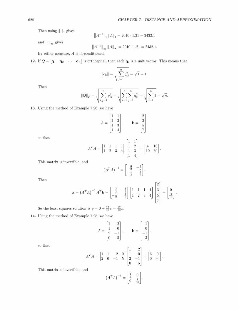
628 CHAPTER 7. DISTANCE AND APPROXIMATION
Then using ‖·‖1 gives ∥∥A−1∥∥
1‖A‖1 = 2010 · 1.21 = 2432.1
and ‖·‖∞ gives ∥∥A−1∥∥∞ ‖A‖∞ = 2010 · 1.21 = 2432.1.
By either measure, A is ill-conditioned.
12. If Q =[q1 q2 · · · qn
]is orthogonal, then each qi is a unit vector. This means that
‖qi‖ =
√√√√ n∑j=1
q2ij =
√1 = 1.
Then
‖Q‖F =
√√√√ n∑i,j=1
q2ij =
√√√√ n∑i=1
n∑j=1
q2ij =
√√√√ n∑i=1
1 =√n.
13. Using the method of Example 7.26, we have
A =
1 11 21 31 4
, b =
2357
,so that
ATA =
[1 1 1 11 2 3 4
]1 11 21 31 4
=
[4 1010 30
].
This matrix is invertible, and (ATA
)−1=
[32 − 1
2
− 12
15
].
Then
x =(ATA
)−1ATb =
[32 − 1
2
− 12
15
][1 1 1 1
1 2 3 4
]2
3
5
7
=
[01710
].
So the least squares solution is y = 0 + 1710x = 17
10x.
14. Using the method of Example 7.25, we have
A =
1 21 02 −10 5
, b =
10−1
3
,so that
ATA =
[1 1 2 02 0 −1 5
]1 21 02 −10 5
=
[6 00 30
].
This matrix is invertible, and (ATA
)−1=
[16 0
0 130
].

Chapter Review 629
Then
x =(ATA
)−1ATb =
[16 0
0 130
][1 1 2 0
2 0 −1 5
]1
0
−1
3
=
[− 1
635
].
15. See Theorem 7.11. With
A =
1 10 11 0
, x =
123
,we have
ATA =
[1 0 11 1 0
]1 10 11 0
=
[2 11 2
],
so that (ATA
)−1=
[23 − 1
3
− 13
23
].
Then the standard matrix of the projection onto the column space W of A is
P = A(ATA
)−1AT =
1 1
0 1
1 0
[ 23 − 1
3
− 13
23
][1 0 1
1 1 0
]=
23
13
13
13
23 − 1
313 − 1
323
,so that the projection of x onto W is
Px =
23
13
13
13
23 − 1
313 − 1
323
1
2
3
=
732353
.16. Note that uuT + vvT =
[u v
] [u v
]T. So we should try A =
[u v
]. Then the column space of
A is span(u,v), so P = A(ATA
)−1AT is the projection matrix onto this span. We now compute P .
First, since u and v are orthonormal,
uTu = u · u = 1, vTv = v · v = 1, uTv = u · v = 0, vTu = v · u = 0.
Then
ATA =
[uT
vT
] [u v
]=
[uTu uTvvTu vTv
]=
[1 00 1
]⇒
(ATA
)−1=
[1 00 1
].
Then the standard matrix of the projection onto the column space of A (which is the space spannedby u and v) is
P = A(ATA
)−1AT = AAT =
[u v
] [uTvT
]= uuT + vvT ,
as required.
17. (a) We have
ATA =
[1 0 11 0 −1
]1 10 01 −1
=
[2 00 2
].
This diagonal matrix has eigenvalues λ1 = λ2 = 2, so the singular values of A are σ1 = σ2 =√
2.

630 CHAPTER 7. DISTANCE AND APPROXIMATION
(b) Compute the corresponding eigenvectors of ATA by row-reduction:[ATA− 2I 0
]=
[0 0 00 0 0
].
So eigenvectors are v1 =
[10
]and v2 =
[01
], and then
V =[v1 v2
]=
[1 00 1
].
To compute U , we have
u1 =1
σ1Av1 =
1√2
1 1
0 0
1 −1
[
1
0
]=
1√2
01√2
u2 =1
σ2Av2 =
1√2
1 1
0 0
1 −1
[
0
1
]=
1√2
0
− 1√2
.
We must extend this to an orthonormal basis of R3; clearly adjoining the vector u3 =
010
is
sufficient. Finally, since Σ must be a 2 × 3 matrix, we append a row of zeroes to the bottom.Then
U =
1√2
1√2
0
0 0 11√2− 1√
20
, Σ =
√
2 0
0√
2
0 0
, V =
[1 0
0 1
]
give an SVD for A, and A = UΣV T .
(c) With Σ as above, we compute Σ+ by transposing Σ and inverting all the nonzero entries:
Σ+ =
[1√2
0 0
0 1√2
0
].
Then
A+ = V Σ+UT =
[1 0
0 1
][1√2
0 0
0 1√2
0
]1√2
0 1√2
1√2
0 − 1√2
0 1 0
=
[12 0 1
212 0 − 1
2
].
18. (a) We have
ATA =
1 11 1−1 −1
[1 1 −11 1 −1
]=
2 2 −22 2 −2−2 −2 2
.The characteristic polynomial is −λ3 +6λ2 = −λ2(λ−6), so λ1 = 6 and λ2 = 0 are the eigenvaluesof ATA. Therefore the singular values of A are σ1 =
√6 and σ2 = 0.
(b) Compute the corresponding eigenvectors of ATA by row-reduction:
[ATA− 6I 0
]=
−4 2 −2 02 −4 −2 0−2 −2 −2 0
→1 0 1 0
0 1 1 00 0 0 0
⇒ x1 =
−1−1
1
[ATA− 0I 0
]=
2 2 −2 02 2 −2 0−2 −2 2 0
→1 1 −1 0
0 0 0 00 0 0 0
⇒ x2 =
−110
, x3 =
101
.

Chapter Review 631
We must orthogonalize {x2,x3}:
x′3 = x3 −〈x2,x3〉〈x2,x2〉
x2 =
1
0
1
− −1
2
−1
1
0
=
1212
1
.
Multiply through by 2 to clear fractions, giving x′′3 =
112
. Finally, normalize all three of these
vectors:
v1 =x1
‖x1‖=
− 1√
3
− 1√3
1√3
, v2 =x2
‖x2‖=
− 1√
21√2
0
, v3 =x′′3‖x′′3‖
=
1√6
1√6
2√6
.Then
V =[v1 v2 v3
]=
− 1√
3− 1√
21√6
− 1√3
1√2
1√6
1√3
0 2√6
.To compute U , we have
u1 =1
σ1Av1 =
1√6
[1 1 −1
1 1 −1
]− 1√
3
− 1√3
1√3
=
[− 1√
2
− 1√2
].
We must extend this to an orthonormal basis of R2; clearly adjoining the vector
u2 =
[1√2
− 1√2
]
is sufficient. Finally, since Σ must be a 2 × 3 matrix, we append two columns of zeroes to theright. Then
U =
[− 1√
21√2
− 1√2− 1√
2
], Σ =
[√6 0 0
0 0 0
], V =
− 1√
3− 1√
21√6
− 1√3
1√2
1√6
1√3
0 2√6
give an SVD for A, and A = UΣV T .
(c) With Σ as above, we compute Σ+ by transposing Σ and inverting all the nonzero entries:
Σ+ =
1√6
0
0 0
0 0
.Then
A+ = V Σ+UT =
− 1√
3− 1√
21√6
− 1√3
1√2
1√6
1√3
0 2√6
1√6
0
0 0
0 0
[− 1√
2− 1√
21√2− 1√
2
]=
16
16
16
16
− 16 − 1
6
.

632 CHAPTER 7. DISTANCE AND APPROXIMATION
19. It suffices to show that the eigenvalues of ATA and those of (PAQ)T (PAQ) are the same. Now,
(PAQ)T (PAQ) = QTATPTPAQ = QT(ATA
)Q
since P is an orthogonal matrix. Thus ATA and (PAQ)T (PAQ) are similar via the matrix Q. ByTheorem 4.22 in Section 4.4, the eigenvalues of ATA are the same as those of (PAQ)T (PAQ), so thatthe singular values of A and PAQ are the same.
20. By the Penrose conditions, we have(A+)2
=(A+AA+
) (A+AA+
)= A+
(AA+
) (A+A
)A+
= A+(AA+
)T (A+A
)TA+
= A+(A+)T (
ATAT) (A+)TA+
= A+(A+)T (
A2)T (
A+)TA+
= A+(A+)TOT
(A+)TA+
= O.

Chapter 8
Codes
8.1 Code Vectors
1. We must have 1 · u = [1, 1, 1, 1, 1] · [1, 0, 1, 1, d] = 0 in Z2. Since this dot product is
1 · 1 + 1 · 0 + 1 · 1 + 1 · 1 + 1 · d = 3 + d = 1 + d in Z2,
we must have d = 1, so that the parity check code vector is v = [1, 0, 1, 1, 1].
2. We must have 1 · u = [1, 1, 1, 1, 1, 1] · [1, 1, 0, 1, 1, d] = 0 in Z2. Since this dot product is
1 · 1 + 1 · 1 + 1 · 0 + 1 · 1 + 1 · 1 + 1 · d = 4 + d = d in Z2,
we must have d = 0, so that the parity check code vector is v = [1, 1, 0, 1, 1, 0].
3. Compute 1 · v:1 · v = 1 · 1 + 1 · 0 + 1 · 1 + 1 · 0 = 2 = 0 in Z2.
Since the sum is zero, a single error could not have occurred.
4. Compute 1 · v:1 · v = 1 · 1 + 1 · 1 + 1 · 1 + 1 · 0 + 1 · 1 + 1 · 1 = 5 = 1 in Z2.
Since the sum is not zero, a single error may have occurred.
5. Compute 1 · v:1 · v = 1 · 0 + 1 · 1 + 1 · 0 + 1 · 1 + 1 · 1 + 1 · 1 = 4 = 0 in Z2.
Since the sum is zero, a single error could not have occurred.
6. Compute 1 · v:
1 · v = 1 · 1 + 1 · 1 + 1 · 0 + 1 · 1 + 1 · 0 + 1 · 1 + 1 · 1 + 1 · 1 = 6 = 0 in Z2.
Since the sum is zero, a single error could not have occurred.
7. We want [1, 1, 1, 1, 1] · [1, 2, 2, 2, d] = 0 in Z3. The dot product is
1 · 1 + 1 · 2 + 1 · 2 + 1 · 2 + 1 · d = 7 + d = 1 + d in Z3,
so the check digit must be d = 2, since 1 + 2 = 0 in Z3.
8. We want [1, 1, 1, 1, 1] · [3, 4, 2, 3, d] = 0 in Z5. The dot product is
1 · 3 + 1 · 4 + 1 · 2 + 1 · 3 + 1 · d = 12 + d = 2 + d in Z5,
so the check digit must be d = 3, since 2 + 3 = 0 in Z5.
633

634 CHAPTER 8. CODES
9. We want [1, 1, 1, 1, 1, 1] · [1, 5, 6, 4, 5, d] = 0 in Z7. The dot product is
1 · 1 + 1 · 5 + 1 · 6 + 1 · 4 + 1 · 5 + 1 · d = 21 + d = d in Z7,
so the check digit must be d = 0.
10. We want [1, 1, 1, 1, 1, 1, 1] · [3, 0, 7, 5, 6, 8, d] = 0 in Z9. The dot product is
1 · 3 + 1 · 0 + 1 · 7 + 1 · 5 + 1 · 6 + 1 · 8 + 1 · d = 29 + d = 2 + d in Z9,
so the check digit must be d = 7, since 2 + 7 = 0 in Z9.
11. Suppose u = [u1, u2, . . . , un], and suppose that v differs from u in exactly one component, say thejth component. Then v = [u1, u2, . . . , vj , . . . , un] where uj 6= vj . So
c · (u− v) = [1, 1, . . . , 1] · ([u1, u2, . . . , uj , . . . , un]− [u1, u2, . . . , vj , . . . , un])
= [1, 1, . . . , 1] · [0, 0, . . . , 0, uj − vj , 0, . . . , 0]
= uj − vj 6= 0.
Thus c · (u− v) 6= 0 so that c · u 6= c · v.
12. With c = [3, 1, 3, 1, 3, 1, 3, 1, 3, 1, 3, 1], we want c · u = 0 in Z10:
c · u = [3, 1, 3, 1, 3, 1, 3, 1, 3, 1, 3, 1] · [0, 5, 9, 4, 6, 4, 7, 0, 0, 2, 7, d]
= 3 · 0 + 1 · 5 + 3 · 9 + 1 · 4 + 3 · 6 + 1 · 4 + 3 · 7 + 1 · 0 + 3 · 0 + 1 · 2 + 3 · 7 + 1 · d= 102 + d = 2 + d in Z10.
So the check digit must be d = 8.
13. With c = [3, 1, 3, 1, 3, 1, 3, 1, 3, 1, 3, 1], we want c · u = 0 in Z10:
c · u = [3, 1, 3, 1, 3, 1, 3, 1, 3, 1, 3, 1] · [0, 1, 4, 0, 1, 4, 1, 8, 4, 1, 2, d]
= 3 · 0 + 1 · 1 + 3 · 4 + 1 · 0 + 3 · 1 + 1 · 4 + 3 · 1 + 1 · 8 + 3 · 4 + 1 · 1 + 3 · 2 + 1 · d= 50 + d = d in Z10.
So the check digit must be d = 0.
14. Let u = [0, 4, 6, 9, 5, 6, 1, 8, 2, 0, 1, 5] and c = [3, 1, 3, 1, 3, 1, 3, 1, 3, 1, 3, 1]. Then
(a) We check if c · u = 0:
c · u = [3, 1, 3, 1, 3, 1, 3, 1, 3, 1, 3, 1] · [0, 4, 6, 9, 5, 6, 1, 8, 2, 0, 1, 5]
= 3 · 0 + 1 · 4 + 3 · 6 + 1 · 9 + 3 · 5 + 1 · 6 + 3 · 1 + 1 · 8 + 3 · 2 + 1 · 0 + 3 · 1 + 1 · 5= 77 = 7 in Z10.
Since the dot product is nonzero, the UPC cannot be correct.
(b) Substituting an unknown digit d for the 6 in the third position, we get
c · u = [3, 1, 3, 1, 3, 1, 3, 1, 3, 1, 3, 1] · [0, 4, d, 9, 5, 6, 1, 8, 2, 0, 1, 5]
= 3 · 0 + 1 · 4 + 3 · d+ 1 · 9 + 3 · 5 + 1 · 6 + 3 · 1 + 1 · 8 + 3 · 2 + 1 · 0 + 3 · 1 + 1 · 5= 59 + 3d = 9 + 3d in Z10.
Solving 9 + 3d = 0 in Z10 gives d = 7, so the correct third digit is 7.

8.1. CODE VECTORS 635
15. Suppose u = [u1, u2, . . . , u12] is a correct UPC, and suppose that v differs from u in exactly onecomponent, say the jth component. Then v = [u1, u2, . . . , vj , . . . , u12] where uj 6= vj . So
c · (u− v) = [3, 1, . . . , 1] · ([u1, u2, . . . , uj , . . . , u12]− [u1, u2, . . . , vj , . . . , u12])
= [1, 1, . . . , 1] · [0, 0, . . . , 0, uj − vj , 0, . . . , 0]
= 1(uj − vj) or 3(uj − vj).
If 1(uj − vj) = 0 ∈ Z10, then uj = vj ∈ Z10. Since both uj and vj are between 0 and 9, they mustbe equal. Similarly, if 3(uj − vj) = 0 ∈ Z10, then since 3x = 0 ∈ Z10 implies that x = 0, we see againthat uj = vj ∈ Z10. So neither of these can be zero, since uj 6= vj . Thus c · (u − v) 6= 0 so that0 = c · u 6= c · v. Since c · v 6= 0, this error will be detected.
16. (a) Compute c · u′, where u′ is the given UPC with the second and third components transposed:
c · u′ = [3, 1, 3, 1, 3, 1, 3, 1, 3, 1, 3, 1] · [0, 4, 7, 9, 2, 7, 0, 2, 0, 9, 4, 6]
= 3 · 0 + 1 · 4 + 3 · 7 + 1 · 9 + 3 · 2 + 1 · 7 + 3 · 0 + 1 · 2 + 3 · 0 + 1 · 9 + 3 · 4 + 1 · 6= 76 = 6 in Z10.
Since the dot product is nonzero, this error will be detected.
(b) Since 3 · 4 + 9 = 21 while 3 · 9 + 4 = 31, and 21 = 31 = 1 in Z10, transposing the third andfourth entries in the UPC will not change the dot product. So this transposition error will not bedetected.
(c) Suppose that transposing ui and ui+1 does not change the dot product, so that if the UPC withthe entries transposed is u′, then c · u = c · u′ = 0. Then
u′ = u + ei(ui+1 − ui) + ei+1(ui − ui+1),
and thus
0 = c · u′ = c · (u + ei(ui+1 − ui) + ei+1(ui − ui+1))
= c · u + c · ei(ui+1 − ui) + c · ei+1(ui − ui+1))
= ci(ui+1 − ui) + ci+1(ui − ui+1)
= ui(ci+1 − ci) + ui+1(ci − ci+1).
If i is even, then ci = 1 and ci+1 = 3, and we get 2ui − 2ui+1 = 2ui + 8ui+1 = 0 in Z10. If i isodd, then ci = 3 and ci+1 = 1, so we get −2ui + 2ui+1 = 8ui + 2ui+1 = 0 in Z10. Note that inpart (b) above, i = 3 is odd, and 8u3 + 2u4 = 8 · 4 + 2 · 9 = 32 + 18 = 50 = 0 in Z10, as expected.
17. Here c = [10, 9, 8, 7, 6, 5, 4, 3, 2, 1] and u = [0, 3, 8, 7, 9, 7, 9, 9, 3, d], so that
c · u = [10, 9, 8, 7, 6, 5, 4, 3, 2, 1] · [0, 3, 8, 7, 9, 7, 9, 9, 3, d]
= 10 · 0 + 9 · 3 + 8 · 8 + 7 · 7 + 6 · 9 + 5 · 7 + 4 · 9 + 3 · 9 + 2 · 3 + 1 · d= 298 + d = 1 + d in Z11.
So the check digit is d = X, since X represents 10, and 1 + 10 = 0 in Z11.
18. Here c = [10, 9, 8, 7, 6, 5, 4, 3, 2, 1] and u = [0, 3, 9, 4, 7, 5, 6, 8, 2, d], so that
c · u = [10, 9, 8, 7, 6, 5, 4, 3, 2, 1] · [0, 3, 9, 4, 7, 5, 6, 8, 2, d]
= 10 · 0 + 9 · 3 + 8 · 9 + 7 · 4 + 6 · 7 + 5 · 5 + 4 · 6 + 3 · 8 + 2 · 2 + 1 · d= 246 + d = 4 + d in Z11.
So the check digit is d = 7, since 4 + 7 = 0 in Z11.

636 CHAPTER 8. CODES
19. (a) Let c be the check vector as in the previous exercise, and let u = [0, 4, 4, 9, 5, 0, 8, 3, 5, 6]. Then
c · u = [10, 9, 8, 7, 6, 5, 4, 3, 2, 1] · [0, 4, 4, 9, 5, 0, 8, 3, 5, 6]
= 10 · 0 + 9 · 4 + 8 · 4 + 7 · 9 + 6 · 5 + 5 · 0 + 4 · 8 + 3 · 3 + 2 · 5 + 1 · 6= 218 = 9 in Z11.
Since the dot product is not zero, this ISBN-10 is not correct.
(b) Substitute an unknown digit d for the 5 in the fifth entry and recompute the dot product:
c · u = [10, 9, 8, 7, 6, 5, 4, 3, 2, 1] · [0, 4, 4, 9, d, 0, 8, 3, 5, 6]
= 10 · 0 + 9 · 4 + 8 · 4 + 7 · 9 + 6 · d+ 5 · 0 + 4 · 8 + 3 · 3 + 2 · 5 + 1 · 6= 188 + 6d = 1 + 6d in Z11.
Solving 1 + 6d = 0 in Z11 gives d = 9. The correct digit was 9.
20. (a) Let u′ be u with the fourth and fifth entries transposed: u′ = [0, 6, 7, 7, 9, 6, 2, 9, 0, 6]. Then
c · (u− u′) = c · [0, 0, 0, 2, −2, 0, 0, 0, 0, 0] = 7 · 2 + 6 · (−2) = 2 6= 0.
So this transposition error will be detected.
(b) See part (c).
(c) A correct ISBN-10 vector u satisfies the check constraint (in Z11)
10∑i=1
(11− i)ui = 0.
Suppose that uj and uj+1 are transposed, giving a new vector u′. Then ui = u′i except for i = jor i = j + 1, so that
c · u′ =
10∑i=1
(11− i)u′i
=
10∑i=1
(11− i)ui − (11− j)uj + (11− j)u′j − (11− (j + 1))uj+1 + (11− (j + 1))u′j+1
= 0 + (11− j)(u′j − uj) + (11− (j + 1))(u′j+1 − uj+1)
= (11− j)(uj+1 − uj) + (10− j)(uj − uj+1)
= uj+1 − uj .
So unless uj and uj+1 are equal, in which case the transposition does not change the vector, theresulting checksum will be nonzero, so the error will be detected.
21. (a) Let c be the ISBN-10 check vector, and let u′ = [0, 8, 3, 7, 0, 9, 9, 0, 2, 6]. Then
c · u′ = [10, 9, 8, 7, 6, 5, 4, 3, 2, 1] · [0, 8, 3, 7, 0, 9, 9, 0, 2, 6]
= 10 · 0 + 9 · 8 + 8 · 3 + 7 · 7 + 6 · 0 + 5 · 9 + 4 · 9 + 3 · 0 + 2 · 2 + 1 · 6= 236 = 5 6= 0 in Z11.
Since the dot product is not zero, this ISBN-10 is not correct.
(b) From part (c) of Exercise 20, the dot product we got in part (a) is the difference (in Z11 of thetwo transposed entries in the correct vector u. So we are looking for two entries u′j = uj+1 andu′j+1 = uj such that
uj+1 − uj = u′j − u′j+1 = 5 in Z11.
The only such pair are the second and third entries, so the correct ISBN-10 must have been[0, 3, 8, 7, 0, 9, 9, 0, 2, 6].
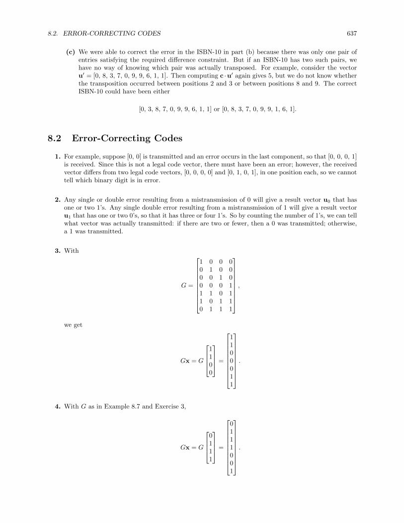
8.2. ERROR-CORRECTING CODES 637
(c) We were able to correct the error in the ISBN-10 in part (b) because there was only one pair ofentries satisfying the required difference constraint. But if an ISBN-10 has two such pairs, wehave no way of knowing which pair was actually transposed. For example, consider the vectoru′ = [0, 8, 3, 7, 0, 9, 9, 6, 1, 1]. Then computing c ·u′ again gives 5, but we do not know whetherthe transposition occurred between positions 2 and 3 or between positions 8 and 9. The correctISBN-10 could have been either
[0, 3, 8, 7, 0, 9, 9, 6, 1, 1] or [0, 8, 3, 7, 0, 9, 9, 1, 6, 1].
8.2 Error-Correcting Codes
1. For example, suppose [0, 0] is transmitted and an error occurs in the last component, so that [0, 0, 0, 1]is received. Since this is not a legal code vector, there must have been an error; however, the receivedvector differs from two legal code vectors, [0, 0, 0, 0] and [0, 1, 0, 1], in one position each, so we cannottell which binary digit is in error.
2. Any single or double error resulting from a mistransmission of 0 will give a result vector u0 that hasone or two 1’s. Any single double error resulting from a mistransmission of 1 will give a result vectoru1 that has one or two 0’s, so that it has three or four 1’s. So by counting the number of 1’s, we can tellwhat vector was actually transmitted: if there are two or fewer, then a 0 was transmitted; otherwise,a 1 was transmitted.
3. With
G =
1 0 0 00 1 0 00 0 1 00 0 0 11 1 0 11 0 1 10 1 1 1
,
we get
Gx = G
1100
=
1100011
.
4. With G as in Example 8.7 and Exercise 3,
Gx = G
0111
=
0111001
.
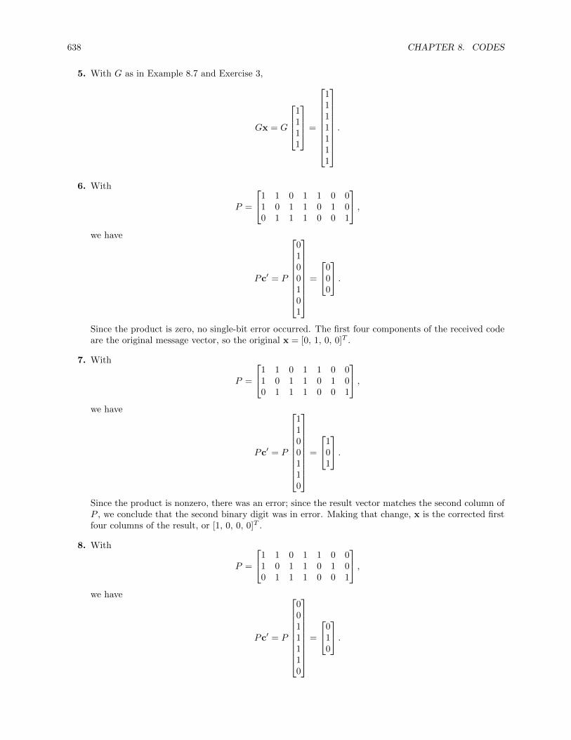
638 CHAPTER 8. CODES
5. With G as in Example 8.7 and Exercise 3,
Gx = G
1111
=
1111111
.
6. With
P =
1 1 0 1 1 0 01 0 1 1 0 1 00 1 1 1 0 0 1
,we have
Pc′ = P
0100101
=
000
.
Since the product is zero, no single-bit error occurred. The first four components of the received codeare the original message vector, so the original x = [0, 1, 0, 0]T .
7. With
P =
1 1 0 1 1 0 01 0 1 1 0 1 00 1 1 1 0 0 1
,we have
Pc′ = P
1100110
=
101
.
Since the product is nonzero, there was an error; since the result vector matches the second column ofP , we conclude that the second binary digit was in error. Making that change, x is the corrected firstfour columns of the result, or [1, 0, 0, 0]T .
8. With
P =
1 1 0 1 1 0 01 0 1 1 0 1 00 1 1 1 0 0 1
,we have
Pc′ = P
0011110
=
010
.

8.2. ERROR-CORRECTING CODES 639
Since the product is nonzero, there was an error; since the result vector matches the sixth column ofP , we conclude that the sixth binary digit was in error. The sixth digit is part of the check code, notof the message, so that the correct message is the first four digits of the result, or x = [0, 0, 1, 1]T .
9. (a) If a = [a1, a2, a3, a4, a5, a6] ∈ Z62 is an arbitrary vector, the encoded vector has a seventh compo-
nent a7 such that∑7i=1 ai = 0 ∈ Z2. This can be encoded using the matrix P = [1, 1, 1, 1, 1, 1, 1],
since
P
a1
a2
a3
a4
a5
a6
a7
=
7∑i=1
ai.
(b) Using the definitions, we have B = [1, 1, 1, 1, 1, 1], n = 7, and k = 6. Then a standard generatormatrix for this code is
[I6B
]=
1 0 0 0 0 00 1 0 0 0 00 0 1 0 0 00 0 0 1 0 00 0 0 0 1 00 0 0 0 0 11 1 1 1 1 1
.
(c) By Theorem 8.1, this is an error-correcting code if and only if the columns of P are nonzero anddistinct. But all the columns of P are the same, so this is not an error-correcting code.
10. (a) The code words are found by multiplying G by each possible input:
[0, 0] → G
[00
]= [0, 0, 0, 0, 0]T
[0, 1] → G
[01
]= [0, 1, 0, 1, 1]T
[1, 0] → G
[10
]= [1, 0, 1, 0, 1]T
[1, 1] → G
[11
]= [1, 1, 1, 1, 0]T .
(b) Here B =
1 00 11 1
, so that the parity check matrix is
P =[B I3
]=
1 0 1 0 00 1 0 1 01 1 0 0 1
.Since the columns of P are nonzero and distinct, this is a single error-correcting code.
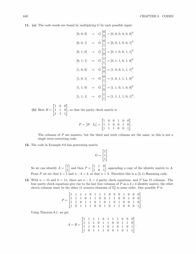
640 CHAPTER 8. CODES
11. (a) The code words are found by multiplying G by each possible input:
[0, 0, 0] → G
[00
]= [0, 0, 0, 0, 0, 0]T
[0, 0, 1] → G
[01
]= [0, 0, 1, 0, 0, 1]T
[0, 1, 0] → G
[10
]= [0, 1, 0, 0, 1, 1]T
[0, 1, 1] → G
[11
]= [0, 1, 1, 0, 1, 0]T
[1, 0, 0] → G
[00
]= [1, 0, 0, 1, 1, 1]T
[1, 0, 1] → G
[01
]= [1, 0, 1, 1, 1, 0]T
[1, 1, 0] → G
[10
]= [1, 1, 0, 1, 0, 0]T
[1, 1, 1] → G
[11
]= [1, 1, 1, 1, 0, 1]T .
(b) Here B =
1 0 01 1 01 1 1
, so that the parity check matrix is
P =[B I3
]=
1 0 0 1 0 01 1 0 0 1 01 1 1 0 0 1
.The columns of P are nonzero, but the third and sixth columns are the same, so this is not asingle error-correcting code.
12. The code in Example 8.6 has generating matrix
G =
111
.So we can identify A =
[11
]and then P =
[1 1 01 0 1
], appending a copy of the identity matrix to A.
From P we see that k = 1 and n− k = 2, so that n = 3. Therefore this is a (3, 1) Hamming code.
13. With n = 15 and k = 11, there are n − k = 4 parity check equations, and P has 15 columns. Thefour parity check equations give rise to the last four columns of P as a 4× 4 identity matrix; the othereleven columns must be the other 11 nonzero elements of Z4
2 in some order. One possible P is
P =
1 1 1 1 0 1 1 1 0 0 0 1 0 0 01 1 1 0 1 1 0 0 1 1 0 0 1 0 01 1 0 1 1 0 1 0 1 0 1 0 0 1 01 0 1 1 1 0 0 1 0 1 1 0 0 0 1
.Using Theorem 8.1, we get
A = B =
1 1 1 1 0 1 1 1 0 0 01 1 1 0 1 1 0 0 1 1 01 1 0 1 1 0 1 0 1 0 11 0 1 1 1 0 0 1 0 1 1
.

8.3. DUAL CODES 641
Therefore the generating matrix for the Hamming (15,11) code is
G =
1 0 0 0 0 0 0 0 0 0 00 1 0 0 0 0 0 0 0 0 00 0 1 0 0 0 0 0 0 0 00 0 0 1 0 0 0 0 0 0 00 0 0 0 1 0 0 0 0 0 00 0 0 0 0 1 0 0 0 0 00 0 0 0 0 0 1 0 0 0 00 0 0 0 0 0 0 1 0 0 00 0 0 0 0 0 0 0 1 0 00 0 0 0 0 0 0 0 0 1 00 0 0 0 0 0 0 0 0 0 11 1 1 1 0 1 1 1 0 0 01 1 1 0 1 1 0 0 1 1 01 1 0 1 1 0 1 0 1 0 11 0 1 1 1 0 0 1 0 1 1
.
14. Suppose that B = A; then
G =
[IkA
], P =
[A In−k
].
Note that A is (n− k)× k. Choose x ∈ Zn2 . Then
PGx =[A In−k
] [IkA
]x = (AIk + In−kA)x = 2Ax.
However, in Z2, 2 = 0, so that 2Ax = 0Ax = 0.
15. Suppose
G =
[IkA
], P =
[A In−k
]are standard generator and parity check matrices for the same code. Choose x ∈ Zk2 , and let c = Gxbe the encoding of x. If there is a transmission error in the ith column of c, receiving c′ instead, thenPc′ = pi. Similarly, if there is a transmission error in the jth column of c, receiving c′′ instead, thenPc′′ = pj . Thus if pi = pj , we cannot tell whether the received vector corresponds to an error in theith or jth column.
8.3 Dual Codes
1. Add column 2 to column 1, giving
G′ =
1 00 11 0
,which is in standard form. Since we did not use R1, this is the same code as C.
2. Perform the following set of column operations:1 0 11 0 00 1 11 1 00 0 1
C1↔C3−−−−−→
1 0 10 0 11 1 00 1 11 0 0
C2↔C3−−−−−→
1 1 00 1 01 0 10 1 11 0 0
.

642 CHAPTER 8. CODES
Continue, adding columns to each other:1 1 00 1 01 0 10 1 11 0 0
C1+C2→C2−−−−−−−−→
1 0 00 1 01 1 10 1 11 1 0
C3+C1→C1−−−−−−−−→
C3+C2→C2−−−−−−−−→
1 0 00 1 00 0 11 0 11 1 0
= G′.
This matrix G′ is in standard form. Since we did not use R1, the code C ′ is the same as the code C.
3. Since the first row of G is zero, we will need to use the operation R1, so the resulting code C ′ will beequivalent to but not equal to C. First exchange the first and fourth rows, then apply the followingcolumn operations:
1 1 11 0 10 1 10 0 0
C1+C2→C2−−−−−−−−→
C1+C3→C3−−−−−−−−→
1 0 01 1 00 1 10 0 0
C3+C2→C2−−−−−−−−→
1 0 01 1 00 0 10 0 0
C2+C1→C1−−−−−−−−→
1 0 00 1 00 0 10 0 0
= G′.
This matrix G′ is in standard form.
4. Since the first and second rows of G are identical, we will need to use the operation R1, so the resultingcode C ′ will be equivalent to but not equal to C. First exchange the first and third rows, then applythe following column operation:
1 01 11 10 01 0
C2+C1→C1−−−−−−−−→
1 00 10 10 01 0
= G′.
This matrix G′ is in standard form.
5. Since there is only one row, and the last entry is not a 1 (the one-dimensional identity matrix), wemust use C1. Interchange the second and third columns, giving
P ′ =[1 0 1
].
This is in standard form; since we used C1, the corresponding code is equivalent to but not equal toC.
6. Perform the following row operations:[1 1 0 11 1 1 1
]R1↔R2−−−−−→
[1 1 1 11 1 0 1
]R2+R1→R1−−−−−−−−→
[0 0 1 01 1 0 1
]= P ′.
This matrix P ′ is in standard form. Since we did not use C1, the corresponding code is equal to C.
7. Since the third and fourth columns of P are identical, we cannot get a 3×3 identity matrix in columnsthree through five without using C1. So the resulting code C ′ will be equivalent to but not equal toC. First exchange columns 1 and 4, and then perform the following row operations:1 1 1 0 0
0 1 0 1 11 0 1 0 1
R1+R3→R3−−−−−−−−→
1 1 1 0 00 1 0 1 10 1 0 0 1
R3+R2→R2−−−−−−−−→
1 1 1 0 00 0 0 1 00 1 0 0 1
= P ′.
This matrix P ′ is in standard form.
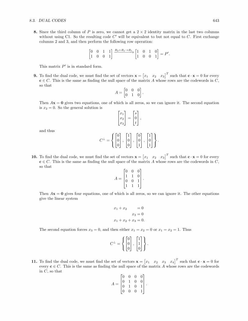
8.3. DUAL CODES 643
8. Since the third column of P is zero, we cannot get a 2 × 2 identity matrix in the last two columnswithout using C1. So the resulting code C ′ will be equivalent to but not equal to C. First exchangecolumns 2 and 3, and then perform the following row operation:[
0 0 1 11 0 0 1
]R2+R1→R1−−−−−−−−→
[1 0 1 01 0 0 1
]= P ′.
This matrix P ′ is in standard form.
9. To find the dual code, we must find the set of vectors x =[x1 x2 x3
]Tsuch that c · x = 0 for every
c ∈ C. This is the same as finding the null space of the matrix A whose rows are the codewords in C,so that
A =
[0 0 00 1 0
].
Then Ax = 0 gives two equations, one of which is all zeros, so we can ignore it. The second equationis x2 = 0. So the general solution is x1
x2
x3
=
s0t
,and thus
C⊥ =
0
00
,1
00
,0
01
,1
01
.
10. To find the dual code, we must find the set of vectors x =[x1 x2 x3
]Tsuch that c · x = 0 for every
c ∈ C. This is the same as finding the null space of the matrix A whose rows are the codewords in C,so that
A =
0 0 01 1 00 0 11 1 1
.Then Ax = 0 gives four equations, one of which is all zeros, so we can ignore it. The other equationsgive the linear system
x1 + x2 = 0
x3 = 0
x1 + x2 + x3 = 0.
The second equation forces x3 = 0, and then either x1 = x2 = 0 or x1 = x2 = 1. Thus
C⊥ =
0
00
,1
10
.
11. To find the dual code, we must find the set of vectors x =[x1 x2 x3 x4
]Tsuch that c · x = 0 for
every c ∈ C. This is the same as finding the null space of the matrix A whose rows are the codewordsin C, so that
A =
0 0 0 00 1 0 00 1 0 10 0 0 1
.

644 CHAPTER 8. CODES
Then Ax = 0 gives four equations, one of which is all zeros, so we can ignore it. The second equationis x2 = 0, and the fourth is x4 = 0. The third is x2 +x4 = 0, which is satisfied by x2 = x4 = 0. Finally,x1 and x3 are arbitrary. Thus
C⊥ =
0000
,
1000
,
0010
,
1010
.
12. To find the dual code, we must find the set of vectors x =[x1 x2 x3 x4 x5
]Tsuch that c · x = 0
for every c ∈ C. This is the same as finding the null space of the matrix A whose rows are thecodewords in C, so that
A =
0 0 0 0 00 1 1 0 11 0 0 1 01 1 1 1 1
.Then Ax = 0 gives four equations, one of which is all zeros, so we can ignore it. The remaining threeequations give the linear system
x2 + x3 + x5 = 0
x1 + x4 = 0
x1 + x2 + x3 + x4 + x5 = 0.
Note that the third equation is the sum of the first two, so we need only consider the first two. Thesecond equation gives x1 = x4, while the first tells us that x2, x3, and x5 must have an even numberof 1’s. Thus
C⊥ =
00000
,
10010
,
01100
,
11110
,
00101
,
10111
,
01001
,
11011
.
13. Let
P⊥ = GT =
[1 1 1 01 1 0 1
].
P⊥ is in standard form, with
A =
[1 11 1
].
Thus
G⊥ =
[IA
]=
1 00 11 11 1
.14. Since
GT =
[1 0 1 1 00 1 0 1 1
]is not in standard form, add the first row to the second; now it is in standard form and
P⊥ =
[1 0 1 1 01 1 1 0 1
].
Then
A =
[1 0 11 1 1
],

8.3. DUAL CODES 645
so that
G⊥ =
[IA
]=
1 0 00 1 00 0 11 0 11 1 1
.15. PT is not in standard form, but adding the second column of PT to the first gives
G⊥ =
1 00 11 01 1
,which is in standard form with
A =
[1 01 1
].
Then
P⊥ =[A I
]=
[1 0 1 01 1 0 1
].
16. PT is not in standard form, but adding the third column of PT to the first gives
G⊥ =
1 0 00 1 00 0 11 0 01 1 1
,which is in standard form with
A =
[1 0 01 1 1
].
Then
P⊥ =[A I
]=
[1 0 0 1 01 1 1 0 1
].
17. By Theorem 8.2,
G⊥ = PT =
1 1 01 0 10 1 11 1 11 0 00 1 00 0 1
, P⊥ = GT =
1 0 0 0 1 1 00 1 0 0 1 0 10 0 1 0 0 1 10 0 0 1 1 1 1
.
18. (a) For E3, the parity check is that the sum of the entries of the codeword is zero, so the parity checkmatrix must be P =
[A I
]=[1 1 1
]. Then A =
[1 1
], so that
G =
[IA
]=
1 00 11 1
.For Rep3, 0 maps to 0 and 1 maps to 1, so the generator matrix must be
G′ =
[IA′
]=
111
, so that A′ =
[11
].

646 CHAPTER 8. CODES
Then
P ′ =[A′ I
]=
[1 1 01 0 1
].
(b) Note that G′ = PT from part (a). While P ′ 6= GT , it can be transformed into GT by adding thesecond row to the first row and then exchanging the first and second rows, so these are paritycheck matrices for the same code.
19. The argument is much the same as in Exercise 18. For En, the parity check is that the sum of theentries of the codeword is zero, so the parity check matrix must be the 1 × n matrix P =
[A I
]=[
1 1 · · · 1]. Then A is the 1× (n− 1) matrix
[1 1 · · · 1
], so that G is the n× (n− 1) matrix
G =
[In−1
A
]=
1 0 0 · · · 00 1 0 · · · 0...
......
. . ....
0 0 0 · · · 11 1 1 · · · 1
.
For Repn, 0 maps to 0 and 1 maps to 1, so the generator matrix must be the n× 1 matrix
G′ =
[IA′
]=
11...1
so that A′ is the (n− 1)× 1 matrix
A′ =
11...1
= AT .
Then P ′ is the (n− 1)× n matrix
P ′ =[A′ In−1
]=
1 1 0 0 · · · 01 0 1 0 · · · 0...
......
.... . .
...1 0 0 0 · · · 1
.We see that G′ = PT and that P ′ can be transformed into GT by adding the last row to each of theother rows and then moving the last row to the first row (this is the same as several row exchanges).Therefore En and Repn are dual codes.
20. We must show that if x ∈ D⊥, then x ∈ C⊥. But x ∈ D⊥ means that d · x = 0 for all d ∈ D. SinceC ⊂ D, certainly also c · x = 0 for all c ∈ C, so that x ∈ C⊥.
21. It suffices to show that if G is a generator matrix for C, then it is also a generator matrix for(C⊥)⊥
.If G is a generator matrix for C, then GT is a parity check matrix for C⊥ by Theorem 8.2(a). Then
by Theorem 8.2(b), we see that(GT)T
= G is a generator matrix for(C⊥)⊥
.
22. Let G and P be generator and parity check matrices for C. We want G⊥ = G. But G⊥ = PT , so wewant G = PT . Since n = 6, it follows from G = PT that n− k = k, so that k = 3. So one such code is
G =
[I3I3
], P =
[I3 I3
].
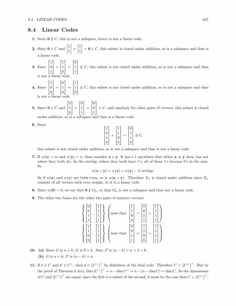
8.4. LINEAR CODES 647
8.4 Linear Codes
1. Since 0 /∈ C, this is not a subspace, hence is not a linear code.
2. Since 0 ∈ C and
[11
]+
[11
]= 0 ∈ C, this subset is closed under addition, so is a subspace and thus is
a linear code.
3. Since
101
+
110
=
011
/∈ C, this subset is not closed under addition, so is not a subspace and thus
is not a linear code.
4. Since
100
+
010
=
110
/∈ C, this subset is not closed under addition, so is not a subspace and thus
is not a linear code.
5. Since 0 ∈ C and
010
+
011
=
001
∈ C, and similarly for other pairs of vectors, this subset is closed
under addition, so is a subspace and thus is a linear code.
6. Since 1010
+
1100
=
0110
/∈ C,
this subset is not closed under addition, so is not a subspace and thus is not a linear code.
7. If w(x) = m and w(y) = n, then consider x + y. It has a 1 anywhere that either x or y does, but notwhere they both do. In the overlap, where they both have 1’s, all of these 1’s become 0’s in the sum.So
w(x + y) = w(x) + w(y)− 2 overlap.
So if w(x) and w(y) are both even, so is w(x + y). Therefore En is closed under addition since Enconsists of all vectors with even weight, so it is a linear code.
8. Since w(0) = 0, we see that 0 /∈ On, so that On is not a subspace and thus not a linear code.
9. The other two bases are the other two pairs of nonzero vectors:
0011
,
1111
note that
1100
=
0011
+
1111
1100
,
1111
note that
0011
=
1100
+
1111
.
10. (a) Since G is n× k, G is 9× 4. Also, P is (n− k)× n = 5× 9.
(b) G is n× k; P is (n− k)× n.
11. If c ∈ C and c′ ∈ C⊥, then c ∈(C⊥)⊥
by definition of the dual code. Therefore C ⊂(C⊥)⊥
. But by
the proof of Theorem 8.4(a), dim(C⊥)⊥
= n−dimC⊥ = n− (n−dimC) = dimC. So the dimensions
of C and(C⊥)⊥
are equal; since the first is a subset of the second, it must be the case that C =(C⊥)⊥
.

648 CHAPTER 8. CODES
12. By Theorem 8.4(b), C has 2k vectors and C⊥ has 2n−k vectors. If C = C⊥, then 2k = 2n−k; multiplythrough by 2k to get 22k = 2n, so that n = 2k is even.
13. Starting with the basis for R2 given in the text,r21 =
1111
, r22 =
0101
, r23 =
0011
,
a basis for R3 is, by the definitions,
{[r21
r21
],
[r22
r22
],
[r23
r23
],
[01
]}=
11111111
,
01010101
,
00110011
,
00001111
.
So the set of vectors in R3 is the subspace generated by this basis, which will have 16 vectors (sincethere are 4 basis elements):
11111111
,
01010101
,
00110011
,
00001111
,
10101010
,
11001100
,
11110000
,
01100110
,
01011010
,
00111100
,
10011001
,
10100101
,
11000011
,
01101001
,
10010110
,
00000000
.
14. (a) Since G0 = 1, we get
G1 =
[G0 0G0 1
]=
[1 01 1
]
G2 =
[G1 0G1 1
]=
1 0 01 1 01 0 11 1 1
G3 =
[G2 0G2 1
]=
1 0 0 01 1 0 01 0 1 01 1 1 01 0 0 11 1 0 11 0 1 11 1 1 1
.
(b) Use induction on n. For n = 1, since the columns of G1 form a basis for R1, we see that G1
generates R1. Now assume Gn−1 generates Rn−1. Then we must show that Gn generates allvectors of the form [
uu
],
[01
],

8.4. LINEAR CODES 649
where u is a basis vector for Rn−1. Let u be a basis vector for Rn−1, and choose x such thatGn−1x = u; such an x exists since Gn−1 generates Rn−1. Then
Gn
[x0
]=
[Gn−1 0Gn−1 1
] [x0
]=
[Gn−1xGn−1x
]=
[uu
]Gn
[01
]=
[Gn−1 0Gn−1 1
] [01
]=
[Gn−10 + 0 · 1Gn−10 + 1 · 1
]=
[01
],
as required.
15. G2 can be put into standard form by the following sequence of column operations:
G2 =
1 0 01 1 01 0 11 1 1
C2+C1→C2−−−−−−−−→
1 1 01 0 01 1 11 0 1
C2+C1→C1−−−−−−−−→
C3+C2→C3−−−−−−−−→
0 1 11 0 00 1 01 0 1
C3+C1→C1−−−−−−−−→
1 1 11 0 00 1 00 0 1
=
[AI
].
This matrix is in standard form, and since we did not use the operation R1, it represents the samecode, namely R2. So A =
[1 1 1
], and thus the associated parity check matrix is
P =[I A
]=[1 1 1 1
].
16. G cannot be put into standard form without using a row operation, since the 4× 4 matrix consistingof the bottom four rows of G has determinant zero. Instead, we use Theorem 8.2: compute a basis
for C⊥ and then a generator matrix G⊥ for C⊥; then(G⊥)T
is a parity check matrix for C, since(C⊥)⊥
= C. Now, C is a four-dimensional subspace of Z72, so its complement is three-dimensional.
Examining the basis of C given in Exercise 13, clearly a basis for C⊥ is
10101010
,
11001100
,
11110000
,
so that G⊥ is the matrix whose columns are these vectors. (Alternatively, if desired one can constructthe matrix whose rows are the entries of the basis for R3 and determine its nullspace, as in the text.)Then
P =(G⊥)T
=
1 0 1 0 1 0 1 01 1 0 0 1 1 0 01 1 1 1 0 0 0 0
.17. Let E ⊆ C be the set of even vectors and O ⊆ C the set of odd vectors. Suppose that O is nonempty,
and choose c0 ∈ O. Consider the map
ψ : E → C : e 7→ c0 + e,
and let O′ = {c0+e : e ∈ E} be the image of this map. Note that ψ is one-to-one, since c0+e1 = c0+e2
implies that e1 = e2.
Claim O′ = O. First, for any e ∈ E,
w(c0 + e) = w(c0) + w(e)− 2 overlap,

650 CHAPTER 8. CODES
from Exercise 7. But w(c0) is odd and w(e) is even, so that w(c0 + e) is odd and therefore c0 + e ∈ O.Thus O′ ⊆ O. Next, choose o ∈ O. Note that c0 + c0 = 0 since we are working in Z2, so that
o = 0 + o = (c0 + c0) + o = c0 + (c0 + o).
But c0 + o ∈ E, since its weight is w(c0) + w(o) − 2 overlap, and all three terms are even. Thuso = c0 + e′ for e′ ∈ E, so that o ∈ O′. Hence O ⊂ O′, so that the O = O′.
Finally, we see that ψ is a one-to-one map from E onto O, so that the two sets have the same numberof elements. Thus exactly have of the code vectors have odd weight.
8.5 The Minimum Distance of a Code
1. Since x− y = x+ y in Z2, we have
dH(x, y) = ‖x− y‖H = ‖x+ y‖H = w(x+ y).
So the distance between two vectors is just the weight of their sum. Denoting by c0, c1, and c2 thevectors in C, we have
w(c0 + c1) = w
010
= 1, w(c0 + c2) = w
110
= 2, w(c1 + c2) = w
100
= 1.
So the minimum distance is d(C) = min(1, 2, 1) = 1.
2. Since x− y = x+ y in Z2, we have
dH(x, y) = ‖x− y‖H = ‖x+ y‖H = w(x+ y).
So the distance between two vectors is just the weight of their sum. Denoting by c0, c1, c2, and c3 thevectors in C, we have
w(c0 + c1) = w
1111
= 4, w(c0 + c2) = w
1001
= 2, w(c0 + c3) = w
0110
= 2,
w(c1 + c2) = w
0110
= 2, w(c1 + c3) = w
1001
= 2, w(c2 + c3) = w
1111
= 4.
So the minimum distance is d(C) = min(2, 4) = 2.
3. Note that
dH
110...0
, 0 = 2,
so that d(C) ≤ 2. Now choose x,y ∈ En, neither of which is the zero vector, with x 6= y. Then sincex + y ∈ En and is nonzero, we know that x + y has at least two ones, so its weight is at least 2.Therefore no pair of nonzero unequal vectors have a distance less than 2, so that d(C) = 2.
4. Since Repn = {0,1}, we see that d(C) = w(0 + 1) = n.

8.5. THE MINIMUM DISTANCE OF A CODE 651
5. The columns of G =
[AI
]form a basis for the code vectors of C. Since no two columns of A are
identical, and the weight of the sum of any two columns of the identity matrix is 2, it follows thatthe weight of the sum of any two columns of G is at least 3. Thus d(C) ≥ 3. But P =
[I A
], and
a1 + a2 + a3 = 0, so by Theorem 8.7, d(C) ≤ 3. Therefore d(C) = 3.
6. It is easy to see that the rows of P are linearly independent (if they were not, the sum of two or threeof them would be zero, and it is not). Therefore rank(P ) = 3, so that the smallest d for which P hasd linearly dependent columns is d = 4, and it follows from Theorem 8.7 that d(C) = 4.
7. Let C = {c1, c2, c3, c4} respectively. Then
dH(c1, c2) = w
01011
= 3, dH(c1, c3) = w
10111
= 4, dH(c1, c4) = w
11100
= 3
dH(c2, c3) = w
11100
= 3, dH(c2, c4) = w
10111
= 4, dH(c3, c4) = w
01011
= 3.
Thus d(C) = 3. Since
dH(c1,u) = w
01010
= 2, dH(c2,u) = w
00001
= 1,
dH(c3,u) = w
11101
= 4, dH(c4,u) = w
10110
= 3,
we conclude that u should decode as c2. Since
dH(c1,v) = w
11010
= 3, dH(c2,v) = w
10001
= 2,
dH(c3,v) = w
01101
= 3, dH(c4,v) = w
00110
= 2,
the identity of v is not determined. It could be decoded as either c2 or c4 using nearest neighbor

652 CHAPTER 8. CODES
decoding. Since
dH(c1,w) = w
10011
= 3, dH(c2,w) = w
11000
= 2,
dH(c3,w) = w
00100
= 1, dH(c4,w) = w
01111
= 4,
we conclude that w should decode as c3.
8. The code generated by (the columns of) G is
C =
0000000
,
1001101
,
0101011
,
0010111
,
1100110
,
1011010
,
0111100
,
1110001
.
Letting the ith element of C be ci, we have:
• min{dH(ci,u)} = 1 only for c5, so that u decodes as c5.
• min{dH(ci,v)} = 1 only for c8, so that v decodes as c8.
• min{dH(ci,w)} = 1 only for c4, so that w decodes as c4.
9. From Exercise 4, d(Repn) = 1, so that Rep8 = {0,1} ⊂ Z82 is such a code.
10. If such a code exists, then its parity check matrix P is (8− 2)× 8 = 6× 8. The rank of such a matrixcan be at most 6, so that the maximum number of linearly independent columns is 6. But that meansthat the minimum number of linearly dependent columns is at most 7. Thus we cannot have d = 8,and such a code cannot exist.
11. If such a code exists, then its parity check matrix P is (8− 5)× 8 = 3× 8. The rank of such a matrixcan be at most 3, so that the maximum number of linearly independent columns is 3. But that meansthat the minimum number of linearly dependent columns is at most 4. Thus we cannot have d = 5,and such a code cannot exist.
12. By Theorem 8.5, R3 is an (8, 4) linear code, and from Example 8.16, it has minimum distance d =23−1 = 4, so it is an (8, 4, 4) linear code.
13. Model the code vectors as four vertices of an octagon. With
c0 =
0000
, c1 =
0101
, c2 =
1010
, c3 =
1111
,we have

8.5. THE MINIMUM DISTANCE OF A CODE 653
c0
c1
c2
c3
14. If c,d ∈ C, then since we are working in Z2, we have c− d = c + d, and then
dH(c,d) = ‖c− d‖H = ‖c + d‖H = w(c + d).
But c + d ∈ C. Thus
dH(C) = min{dH(c,d) : c,d ∈ C} = min{w(c + d) : c,d ∈ C} = min{w(c) : c ∈ C, c 6= 0}.
15. A parity check matrix for any linear (n, k) code is (n − k) × n, so that rank(P ) 6= n − k. Then thenumber of linearly independent columns of P is at most n−k, so that the minimum number of linearlydependent columns is at most n− k + 1. Thus d ≤ n− k + 1, so that d− 1 ≤ n− k.
16. From the previous exercise, we know that d ≤ n − k + 1, so that n − k ≥ d − 1. Now, if every set ofn − k columns of P are linearly independent, then n − k < d. Together, these two inequalities forcen− k = d− 1, or d = n− k + 1. Conversely, if d = n− k + 1, then Theorem 8.7 says that n− k + 1 isthe smallest integer for which P has that many linearly dependent columns. But if this is true, thenit must be the case that every set of n− k columns is linearly independent.