competitive prices and organizational...
TRANSCRIPT

Competitive Prices and Organizational
Choices∗
Patrick Legros† and Andrew F. Newman‡
January 2008
∗Some of the material in this paper circulated in as earlier paper circulated underthe title “ Managerial Firms, Organizational Choice, and Consumer Welfare.” We thankRoland Benabou, Patrick Bolton, Phil Bond, Estelle Cantillon, Jay Pil Choi, MathiasDewatripont, Robert Gibbons, Oliver Hart, Georg Kirchsteiger, Giovanni Maggi, ArminSchmuckler, George Symeonidis for helpful discussion. Legros benefitted from the finan-cial support of the Communaute Francaise de Belgique (projects ARC 98/03-221 andARC00/05-252), and EU TMR Network contract noFMRX-CT98-0203. Newman was theRichard B. Fisher Member of the Institute for Advanced Study, Princeton when some ofthe research for this paper was conducted.†ECARES, Universite Libre de Bruxelles, and CEPR.‡Boston University and CEPR.
1

Abstract
We construct a price-theoretic model of integration decisions and
show that these choices may adversely affect consumers, even in the
absence of monopoly power in supply and product markets. A key
observation is that the price of output helps to determine the orga-
nizational form chosen. At low prices, managers may be resistant
to integration, even if it efficiently coordinates decisions, because it
imposes high privates costs on them. At higher prices, they may
choose integration even if nonintegration would produce more output,
because nonintegration leads to an undesired distribution of private
costs. Moreover, organizational choices affect output and therefore
prices. Since shocks to industries affect product prices, reorganiza-
tions are likely to take place in coordinated fashion and be industry
specific, consistent with the evidence. We show that there are in-
stances in which entry of suppliers can hurt consumers by changing
the terms of trade in the supplier market, thereby inducing harmful
reorganizations. When firms are publicly held, we identify conditions
under which hostile (shareholder initiated) versus friendly (manager
initiated) takeovers are more likely.
2

1 Introduction
Do consumers have an interest in the internal organization of the firms that
make the products they buy? Conventional economic wisdom says no, at
least if product markets are characterized by a reasonable degree of competi-
tion: firms that fail to deliver the goods at the lowest feasible cost, whatever
the reason, including inappropriate organization, will be supplanted by their
more efficient competitors.1
There are, of course, potential interest conflicts between the firm and the
consumer: this is a central concern of the industrial organization literature
and of competition policy. But the predominant view of the firm there is
the classical one of the unitary profit maximizer; as a consequence, the ef-
fects of organizational design on market performance are generally absent
from the analysis, and both the economic literature and policy practice have
focused instead on the adverse effects of market power. In this context,
mergers or other major reorganizations are worthy of concern only insofar
as they increase the firm’s market power. In particular, it would be hard
from this point of view to see how firms might be characterized by too little
integration, something for which there is at least some evidence (Bertrand
and Mullainathan, 2003).
The question is still open whether and how organizational decisions can
affect consumer welfare in ways that do not involve market power. The
key insight is provided by the recent literature on the firm (Grossman and
Hart 1986; Hart and Moore 1990; Hart and Holmstrom 2002), which views
organizational decisions as the purview of managers who trade off the usual
pecuniary costs and benefits, such as profits, with non contractable ones such
as managerial effort, working conditions, corporate culture, or leadership
vision.
The thrust of this literature is that in environments with imperfect or
incomplete contracting, managerial firms may make organizational decisions
that have little to do with profit maximization and/or the interests of share-
holders. In this paper we will show that organizational decisions are influ-
1For instance, as Fama and Jensen (1983) aver, “the form of organization that survives...is the one that delivers the product demanded by customers at the lowest price whilecovering costs.”
3
enced by product prices, and that these decisions in turn determine product
market outcomes. Even in a competitive world, inefficiencies are likely to be
significant: both too much and too little integration are possible outcomes
from the consumer point of view.
To make this point as simply as possible, we rule out market foreclosure
effects altogether by assuming competitive product and supplier markets. In
the model we consider, production of consumer goods requires the combina-
tion of exactly two complementary suppliers, each consisting of a manager
and his collections of assets.2 When the suppliers form a joint enterprise (or
“firm”), the managers operate the assets by taking noncontractable decisions.
As in some recent models of firms, in particular Hart and Holmstrom
(2002), the production technology essentially involves the adoption of stan-
dards. While there is no objectively “right” decision, output is higher on
average the more decisions are in the same direction. The problem is that
managers disagree about which direction they ought to go. Each party will
find it costly to accommodate the other’s approach, but if they don’t agree
on something, the market will be poorly served.
Under nonintegration, managers make their decisions separately, and this
may lead to inefficient production. Integration solves this problem by bring-
ing in an additional party, called HQ, which is motivated by monetary com-
pensation to maximize the enterprise’s output.3 HQ accomplishes this by
enforcing a common standard. But delegating decision rights to HQ does
not come for free, and generates two types of losses. First this solution to
the coordination problem may lead to high private costs for the initial man-
agers. Second, using HQ to enforce coordination may have direct costs in
terms of foregone output. For instance, HQ may not be specialized in all the
tasks carried out by the suppliers, (e.g., Hart and Moore 1999), there may
be additional communication and delay costs (e.g., Radner 1993, Bolton and
Dewatripont 1994), or HQ may have its own moral hazard problems.
Whether to integrate is decided by managers when the firms form; this
2The model is inspired by earlier work (Legros and Newman 1996, forthcoming) thatshows how competitive market conditions determine organizational design such as thedegree of monitoring or the allocation of control. Those papers do not consider the inter-action of organization with the product market or consumer welfare, however.
3Other models that take this view of integration include Alchian and Demsetz (1972),Hart and Holmstrom (2002), Mailath et al. (2002).
4

takes place in a competitive supplier market in which the two types of sup-
pliers “match”. The firms’ output is sold in a competitive product market,
wherein all firms and consumers are price-takers.
At low prices, managers do not value the increase in output brought by
integration since they are not compensated sufficiently for the high costs
they have to bear. At very high prices, managers value output so much
that they are willing to concede in order to achieve coordination. Therefore
integration only emerges for intermediate levels of price. In other words,
there is an inverted U-shaped relationship between product price and the
degree of integration.
One feature of our model is that the derivation of equilibrium organiza-
tional choices and product prices reduces to a standard supply-and-demand
analysis, where the industry supply curve embodies the price dependent or-
ganizational decisions described above. We apply this framework to show
how internal organization, as well as prices and quantities, respond to shocks
such as changes in product demand, entry of additional suppliers. Incorpo-
rating organizational design into this otherwise standard analysis can lead
to surprising results: for instance we identify regimes where product prices
increase and consumer welfare decreases following positive shocks, such as
the entry of low-cost suppliers.
The price mechanism also provides a natural explanation for the tendency
for organizational restructuring to be widespread. There is considerable evi-
dence that firms integrate (or divest) in “waves” and that reorganizations of
this sort are most pronounced at the industry level. Since product price is
common to a whole industry, anything that changes it will not only have the
classical price-theoretic quantity and consumer welfare effects, but will have
organizational effects as well. And as we have suggested, these organizational
effects will in turn feed back to quantity and welfare.
For most of the paper, we are silent about whether the initial units are
publicly owned. If they are, outside shareholders have – in our competitive
world – nearly the same interests as consumers. In particular, at (moder-
ately) low prices, they would also like integration, since from their point of
view there would be an increase in revenue. Thus, the model identifies sit-
uations in which firms are ripe for “takeover”. This begs the question of
whether outside shareholders can discipline managers into taking the profit
5

maximizing organizational decision. Short of imposing such decision directly,
we show that instruments such as variable profit shares or free cash flow will
not eliminate the inefficiencies – and in some cases make things worse.
2 Model
There are two types of supplier, denoted A and B. Production of marketable
output requires the coordinated input of exactly one A and one B provider,
and we call their union a firm. Examples of A and B might include game
consoles and game software, upstream and downstream enterprises, or man-
ufacturing and customer support. For each provider, a decision is rendered
indicating the way in which production is to be carried out. For instance
software can be elegant or user friendly, or a product line and its associ-
ated marketing campaign can be mass- or niche-market oriented. Denote the
decision in an A provider by a ∈ [0, 1], and a B decision by b ∈ [0, 1]. Over-
seeing each provider is a manager, who bears a private cost of the decision
made in his unit. We assume that the A manager’s preferences are increas-
ing in a, while the B manager’s preferences are decreasing in b: formally,
CA(a) = 12(1− a)2 for the manager A and CB(b) = 1
2b2 for manager B.4
It is important that decisions made in each part of the firm do not conflict,
else there is loss of output. More precisely, the enterprise will succeed with a
probability equal to 1− 12(a− b)2, in which case it generates a unit of output;
otherwise it fails, yielding 0. For instance, if A finds Macintosh aesthetically
pleasing while B finds PCs practical, and each adopt large quantities of
their preferred machines, the resulting incompatibilities will reduce expected
output.
Decisions are not contractible, but the right to make them can be reas-
signed by contract. In addition, the output generated by the firm is con-
tractible, which allows monetary incentives to be created. Managers bear
the cost of decisions even if they don’t make them because their primary
function is to implement decisions and to convince their workforces to agree.
Managers can integrate by engaging the service of a headquarters (HQ).
4Although we model the managers disagreement as differences in preferences, we expectvery similar results could be generated by a model in which they differ in “vision” as invan den Steen (2005).
6

HQ can aid in coordinating decisions, but the cost of ceding control from
the managerial point of view is a loss of “quiet life,” that is to say, a higher
private cost. From the consumer point of view, the benefit of integration is
to improve coordination and therefore increase output and decrease prices;
but since they don’t choose organization, they may not enjoy these benefits.
The divergence between consumer and managerial interests is governed
by the efficacy of HQ. Typically, employing an HQ comes at a cost in terms
of foregone output that we model as reduction σ ≥ 0 in the success prob-
ability. As discussed in the Introduction, HQ may reduce potential output
through the direct costs of communication, additional management person-
nel, or losses from delegating decisions from A and B to staff who are not
experts. In this case, HQ could take a share of the (reduced) revenue, leaving
the residual for the managers to share.5
Other costs could be linked to a moral hazard problem: since HQ has
control over both suppliers resources, it also may have opportunities to di-
vert those resources into other activities (including private benefits, other
divisions, or pet projects).6
To summarize, expected output is
Q(a, b) =
1− 12(a− b)2 if there is nonintegration
[1− 12(a− b)2](1− σ) if there is integration.
Before production, B managers match withAmanagers in order to benefit
from the synergies; at the time of matching, they sign contracts indicating
• the share s of managerial revenue accruing to manager A, with 1 − sgoing to B (in case of failure each receives zero); and
5There is an alternative form of integration which does without HQ, instead delegatingfull control to one of the managers, who will subsequently perfectly coordinate the decisionsin his preferred direction. It is straightforward to show (section 2.2) that this form ofintegration is dominated by nonintegration
6For instance, suppose that after output is realized, there is a probability σ that HQhas a chance to divert whatever output there is to an alternative use valued at ν timesits market value, where σ < ν < 1. If output is diverted, it doesn’t reach the market, andthe verifiable information is the same as if the firm had failed. Managers could preventdiversion by offering a share ν to HQ, leaving (1− ν) of the revenue to be shared betweenthe managers, but since ν > σ, it is actually better for them to give HQ a zero share ofmarket revenue and let him divert when he is able, so that successfully produced outputreaches consumers only (1− σ) of the time.
7
• the ownership structure of the relationship.
For now we take the total managerial revenue in case of success to be the
product market price P .
There are only two relevant structures to consider here: nonintegration
(N), where each manager takes the decision on his activity, and integration
(I), where the headquarters HQ takes decisions on each activity. Once a
contract is given, managers (or HQ) make their decisions, output is realized
and shares are distributed.
The demand side of the product market is modelled as a decreasing de-
mand function D(P ), and the market price P is taken as given by all firms
when they make decisions.
In the supplier market, there is a continuum of both types of suppliers.
The A’s are on the long side of the market: their measure is n > 1, while the
B’s have unit measure. All unmatched A managers receive a payoff of zero
(the outside option of B-managers will play little role here and can be taken
to be 0).7
2.1 Integration
With integration, HQ receives an expected surplus proportional to (1− 12(a−
b)2)P and therefore makes decisions for both activities in order to maximize
profits of the integrated firm, that is chooses a = b. When a = b, total cost
is lowest when a = 1/2 and we assume that HQ will choose these decisions
(indeed this is exactly what A and B would want her to do: since it maximizes
the joint payoff, which is perfectly transferable via the sharing rule s, it Pareto
dominates any other choice). The cost to each manager is then 18, and the
payoffs to the A and B managers are
uIA(s, P ) = (1− σ)sP − 1
8
uIB(s, P ) = (1− σ)(1− s)P − 1
8.
Total managerial welfare under integration is W I(P ) = (1− σ)P − 14
and is
fully transferable.
7In fact it is a simple matter to generalize the model to the case of non zero and evenheterogenous outside options, see Section 3.2 and the Appendix.
8

2.2 nonintegration
Since each manager keeps control of his activity, A chooses a ∈ [0, 1] , B
chooses b ∈ [0, 1] in Cournot-Nash fashion. Using the expression for output
under nonintegration yields payoffs
uNA = (1− 1
2(a− b)2)sP − 1
2(1− a)2
uNB = (1− 1
2(a− b)2)(1− s)P − 1
2b2.
The best responses in the (unique) Nash equilibrium are:
aN =1 + (1− s)P
1 + P(1)
bN =(1− s)P
1 + P. (2)
Note that aN > bN and that the coordination loss is
aN − bN =1
1 + P, (3)
which is independent of s. This loss is decreasing in the price P : as P becomes
larger, the revenue motive becomes more important for managers and this
pushes them to better coordinate.
The Nash equilibrium output is
QN(P ) = 1− 1
2(1 + P )2(4)
and the equilibrium payoffs are
uNA (s, P ) = QN(P )sP − 1
2s2
(P
1 + P
)2
(5)
uNB (s, P ) = QN(P )(1− s)P − 1
2(1− s)2
(P
1 + P
)2
.
Varying s, one obtains the Pareto frontier in the case of nonintegra-
tion. We have ∂uA/∂s = QN(P )P − s(
P1+P
)2, ∂uB/∂s = −QN(P )P +
(1 − s)(
P1+P
)2and simple computations show that the Pareto frontier is
decreasing and concave.
9

Total welfare is
WN(s, P ) = QN(P )P − 1
2(s2 + (1− s)2)
(P
1 + P
)2
(6)
The maximum surplus is obtained at s = 1/2 and the minimum surplus
is obtained at s = 0 (or s = 1). Note that when s = 0, a = 1: the A manager
makes no concession, and only the B bears a positive private cost.8
2.3 Choice of Organizational Form
The frontier under integration is a straight line, while the frontier under
nonintegration is concave. The relative positions of these frontiers depend
on the price. Figure 1 below represents a situation where neither integration
nor nonintegration dominates globally, but one form may dominate for some
levels of payoffs. If the frontiers are as in the figure, the organization that
managers choose depend on where they locate along the frontiers, i.e., on the
terms of trade on the supplier market.
As the following proposition establishes, nonintegration may dominate in-
tegration when product price is low or high, but integration never dominates
nonintegration. There is a range of prices where integration is preferred to
nonintegration when B’s share of surplus is large enough. Thus, organiza-
tional form is determined only in the full general equilibrium of the supplier
and product markets.
Contrary to managers, consumers are indifferent between all values of
s given the organization. Hence, conditions in the supplier market affect
consumers only insofar as they affect the choice of organizations.
Proposition 1 When σ is positive, managerial welfare with integration
(i) is smaller than the minimum total welfare with nonintegration if and only
if P does not belong to the interval [π(σ), π(σ)] , where π(σ) and π(σ) are the
two solutions of the equation σ = P−14P (1+P )
.
(ii) is smaller than the maximum welfare with nonintegration.
8Using WN (0, P ) = P(
1− 12(1+P )2
)− 1
2
(P
1+P
)2
, it is now straightforward to showthat giving B full control will be dominated by nonintegration. For under B control,a = b = 0 and even assuming no additional integration cost, the total surplus is P − 1
2which is everywhere less than WN (0, P ).
10

uA
uB
Integration
nonintegration
Figure 1: Frontiers
It is straigthforward to see that [π(σ), π(σ)] is nonempty when σ is smaller
than some upper bound σ, and that π(σ) is increasing and π(σ) is decreasing
in σ.
2.4 Industry Equilibrium and the “Organizationally
Augmented” Supply
Industry equilibrium comprises a general equilibrium of the supplier mar-
ket and product market. In the supplier market, an equilibrium consists of
matches of one upstream firm and one downstream firm, along with a surplus
allocation among all the managers. Such an allocation must be stable in the
sense that no (A,B) pair can form an enterprise that generates payoffs to
each manager that exceed their equilibrium levels. In the product market,
the large number of firms implies that the industry supply is almost surely
equal to its expected value of output given the product price; equilibrium
requires that the the price adjust so that the demand equal the supply.
Since the A agents are in excess supply and would earn zero if unmatched,
their competitive payoff must be equal to zero. Then if frontiers are as in Fig-
11
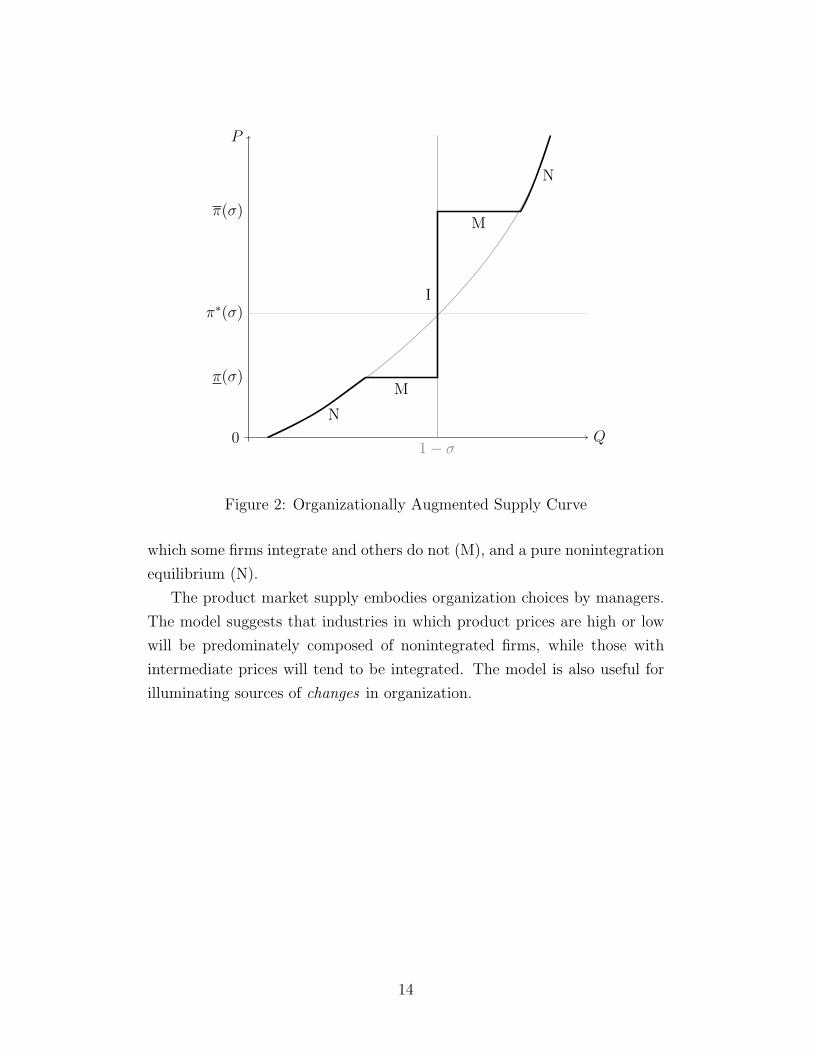
ure 1, integration would be chosen since it maximizes B’s payoff given that
A gets zero. At other product prices, the maximum payoff to B may be gen-
erated through nonintegration. The maximum payoff to B under integration
is equal to the total welfare (1−σ)P− 14
and the maximum payoff to B under
nonintegration obtains when s = 0 in (6), that is (1− 12(1+P )2
)P − 12( P
1+P)2.
From Proposition 1, there are three cases of interest, depending on the
size of σ. When σ = 0, managers (strictly) prefer nonintegration if and only if
P < π(0) = 1. When σ ∈ (0, σ), managers prefer nonintegration if and only
if P /∈ [π(σ), π(σ)] . And when σ > σ, managers never integrate. Integration
will be chosen by managers in equilibrium only when P ∈ [π(σ), π(σ)] .
We note that output supplied to the product market under integration
(1− σ) is smaller than output under nonintegration (1− 12(1+P )2
) if and only
if
σ >1
2(1 + P )2, (7)
that is when
P > π∗(σ) =
√1
2σ− 1. (8)
It is straightforward to see that π∗(σ) ∈ (π(σ), π(σ)) whenever σ < σ.
The reason nonintegration generates higher output as price increases is
simple enough: the higher is P, the more revenue figures in managers’ payoffs.
This leads one to “ concede” to the other’s decision in order to reduce output
losses.
The nonmonotonicity of managers’ organizational preference in price when
σ ∈ (0, σ) is more subtle. At low prices, despite integration’s better output
performance, revenue is still small enough that the managers (in particular
the manager of B) are more concerned with their private benefits, i.e., they
like the quiet life. At high prices, nonintegration performs well enough in
the output dimension that they do not want to incur the cost σ of HQ. Only
for intermediate prices do managers prefer integration. In this range, the B
manager knows that revenue is large enough that he will be induced to bear
a large private cost to match the perfectly self indulgent A manager, who
generates little income from the firm (s = 0) and therefore chooses a = 1. B
prefers the relatively high output and moderate private cost that he incurs
12

under integration.9
As discussed above, the demand side of the product market is represented
by the demand function D(P ). To derive industry supply, suppose that a
fraction α of firms are integrated and a fraction 1 − α are nonintegrated.
Total supply at price P is then
S(P, α) = α(1− σ) + (1− α)
(1− 1
2
(1
1 + P
)2). (9)
For σ < σ, when P < π(σ), α = 0 and total supply is just the output
when all firms choose nonintegration. At P = π(σ), α can vary between 0
and 1 since managers are indifferent between the two forms of organization;
however because π(σ) < π∗(σ), output is greater with integration and as
α increases total supply increases. When α = 1 output is 1 − σ and stays
at this level for all P ∈ (π(σ), π(σ)). At P = π(σ), managers are again
indifferent between the two ownership structures and α can decrease from
1 to 0 continuously; because π∗(σ) < π(σ), output is greater the smaller is
α. Finally for P > π(σ) all firms remain nonintegrated and output increases
with P.
When σ ≥ σ, managers always choose nonintegration and α = 0 for all
prices.
We therefore write S(P, α(P )) to represent the supply correspondence,
where α(P ) is described in the previous paragraph. The supply curve for the
case σ ∈ (0, σ) is represented in Figure 2. The dotted curve corresponds to
the industry supply when no firms are integrated.
An equilibrium in the product market is a price and a quantity that equate
supply and demand: D(P ) ∈ S(P, α(P )). There are three distinct types of
industry equilibria, depending on where along the supply curve the equilib-
rium price occurs: those in which firms integrate (I), the mixed equilibria in
9 For this outcome, it is crucial that the supplier market be ”unbalanced,” i.e., that A orB be accruing the preponderence of the surplus. For as we already noted, the total surplusunder nonintegration when it is equally shared (s = 1
2 ) always exceeds that generated byintegration. Thus if surplus is (nearly) equally shared by A and B,(for instance, if oneside has a nonzero outside option), they never integrate. On the other hand, our specificfunctional forms are not critical to this kind of outcome: similar results obtain if themanagers have a standard partnership problem, where total net revenue is Pf(a, b) andthe non-contractible cost functions CA(a) and CB(b) are increasing in a and b. Details arein the Appendix.
13
0 Q
P
1− σ
π∗(σ)
π(σ)
π(σ)
N
M
I
M
N
Figure 2: Organizationally Augmented Supply Curve
which some firms integrate and others do not (M), and a pure nonintegration
equilibrium (N).
The product market supply embodies organization choices by managers.
The model suggests that industries in which product prices are high or low
will be predominately composed of nonintegrated firms, while those with
intermediate prices will tend to be integrated. The model is also useful for
illuminating sources of changes in organization.
14

3 Comparative Statics
The fact that all firms face the same price means that anything that affects
that price – a demand shift or foreign competition – can lead to widespread
and simultaneous reorganization, e.g., a merger wave or mass divestiture.
An additional channel of coordinated reorganization is the supplier market:
changes in the relative scarcities of the two sides, or to outside opportunities
on one side, will change the way surplus is divided between managers, and
this too will lead to reorganization.10 In some cases these changes in the
supplier market terms of trade will have surprising effects on product market
outcomes.
3.1 Demand and Balanced Supply Shocks
Assume that both sides of the supplier market expand so as to keep the ratio
of A’s to B’s the same, or alternatively assume that the measure of B firms
increases while remaining less than that of A firms. This increase in the
number of A and B firms could come from “globalization”, i.e., a lowering
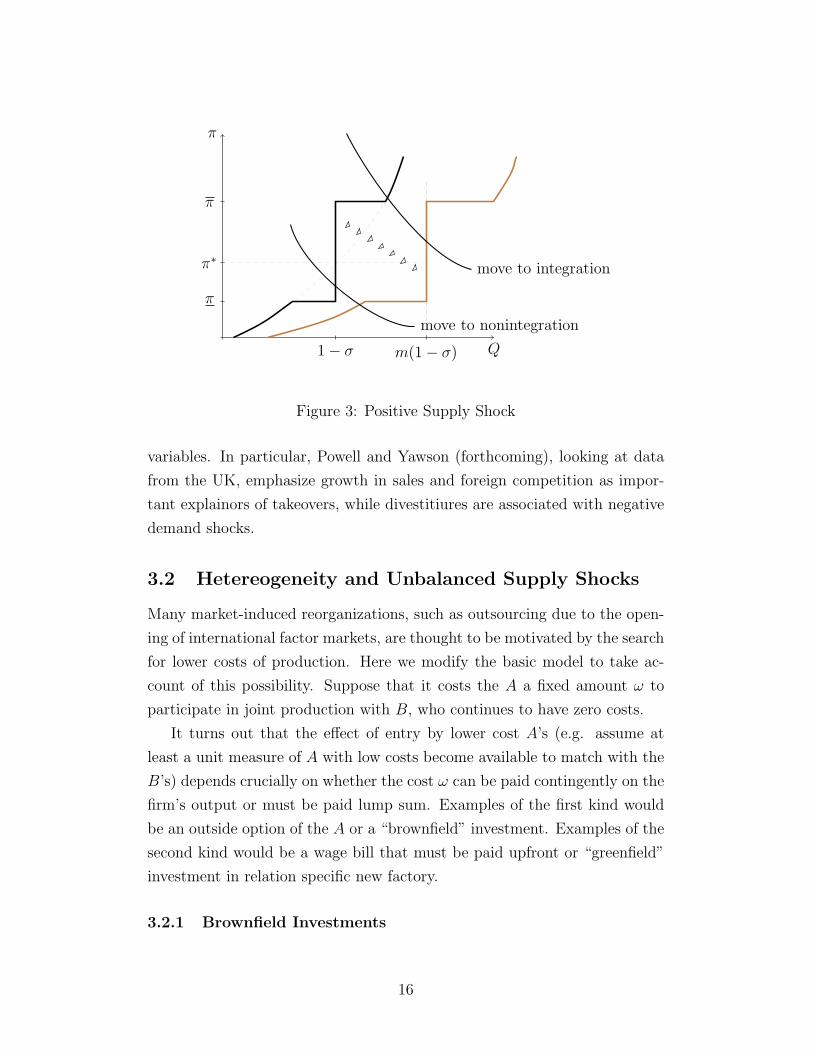
of barriers to international trade and factor movements. See Figure 3. If
demand is high, following the increase in supply, the industry moves from a
nonintegration equilibrium to an integration equilibrium. Hence, in indus-
tries when demand is high and firms are nonintegrated, balanced positive
supply shocks yield merger activity. Hence, globalization can be a force for
the generation of merger activity without further assumption about changes
to technology or regulation. If demand is low however, the opposite is true
and globablization can be a force for divestiture.
Notice that in both cases, though prices fall following entry, they do
not fall as far as they might if somehow the managers were prevented from
integrating when demand is high or forced to stay integrated when demand
is low.
A number of authors have emphasized the empirical regularities surround-
ing “ clustering” of takeovers and divestitures. For instance, Mitchell and
Mulherin (1996) argue that for the US at least, merger waves are best ex-
plained empirically by the joint effects of macroeconomic and industry-level
10See Legros and Newman (forthcoming) for a detailed analysis of this mechanism.
15
Q
π
1− σ m(1− σ)
π∗
π
π
move to integration
move to nonintegration
Figure 3: Positive Supply Shock
variables. In particular, Powell and Yawson (forthcoming), looking at data
from the UK, emphasize growth in sales and foreign competition as impor-
tant explainors of takeovers, while divestitiures are associated with negative
demand shocks.
3.2 Hetereogeneity and Unbalanced Supply Shocks
Many market-induced reorganizations, such as outsourcing due to the open-
ing of international factor markets, are thought to be motivated by the search
for lower costs of production. Here we modify the basic model to take ac-
count of this possibility. Suppose that it costs the A a fixed amount ω to
participate in joint production with B, who continues to have zero costs.
It turns out that the effect of entry by lower cost A’s (e.g. assume at
least a unit measure of A with low costs become available to match with the
B’s) depends crucially on whether the cost ω can be paid contingently on the
firm’s output or must be paid lump sum. Examples of the first kind would
be an outside option of the A or a “brownfield” investment. Examples of the
second kind would be a wage bill that must be paid upfront or “greenfield”
investment in relation specific new factory.
3.2.1 Brownfield Investments
16

Think of contracting with an A manager with a plant that could fetch a
profit of ω in some other use. The contracting problem is very similar to
what we have done before with the caveat that A must now be assured of an
expected payoff of ω.
As is apparent from Figure 1, as the minimum payoff to A decreases, it
becomes possible (and optimal for the B) to choose integration. Formally,
fix the price P and suppose that B’s maximum payoff when A’s cost is ω is
obtained for a sharing rule s, and therefore that the indirect payoffs are
uNA (s, P ) = ω, uNB (s, P ) = WN(s, P )− ω.
Consider now a lower value ω′ < ω. We know that WN(s, P ) and that
uNA (s, P ) are decreasing in s for s < 1/2. Hence, for s′ < s such that
uNA (s′, P ) = ω′, we have WN(s′, P ) < WN(s, ω). Supposing that B is indif-
ferent between nonintegration and integration under ω, we have WN(s, P ) =
(1− σ)P − 1/4, implying that
WN(s′, P )− ω′ < WN(s, P )− ω′
= W I(P )− ω′
and B strictly prefers integration to nonintegration. Hence, whenever P is
such that integration is preferred under ω, it will be also under ω′; because
the preference is strict with ω′ when there is indifference with ω, there are
more prices for which integration is preferred under ω′. Thus, for brownfield
investments, reduced costs are a force toward integration. This is represented
in the Figure 4.
It is then immediate that if the industry demand is high, offshoring brown-
field investments will lead to a lower quantity and higher price with ω′ than
with ω. When demand is low, though, entry of low-cost A’s yields the the
usual comparative static of lower prices and higher quantities.
Note that the payoff of A is adjusted by using the sharing rule only.
Even if the two managers are liquidity constrained, it is possible for them
to borrow ω, transfer ω to A in order to meet the cost of participation and
then commit to repay a debt when output is high. It can be shown, however,
that the payoffs obtained under such debt contracts are Pareto dominated
17
Q
P
Figure 4: Entry of lower cost suppliers: Brownfield investments
by contracts without debt, and will therefore never be used for brownfield
investments (Legros and Newman forthcoming.)
For greenfield investments however, liquidity constrained managers are
forced to borrow ω, since ω must be paid before production takes place.
What is perhaps surprising is that conditional on debt in order to finance the
cost ω, the comparative statics of a lowering of this cost are opposite to the
case of brownfield investment: lower costs are a force toward nonintegration.
3.2.2 Greenfield Investments
If ω must be paid up front, and if the firm has not enough cash for this, the
firm will need to borrow ω from the financial market in exchange for a state
contingent debt repayment D in case of success and 0 in case of failure. The
market for loans is competitive. Under integration, the level of price does
not affect the probability of success and the probability of repayment is one;
the B manager’s surplus is therefore uIB(P, ω) = (1 − σ)P − 1/4 − ω, as in
the brownfield case.
Under nonintegration however, debt distorts incentives to concede and
therefore, if B was indifferent between integration and nonintegration, he will
18
favor nonintegration after a decrease in ω. This is shown in the Appendix.
With greenfield investments, a lower cost faced by the A managers is a
force away from integration. Alternatively the interval [π(σ), π(σ)] over wich
integration is preferred to nonintegration is decreasing in ω (that is the lower
bound increases and the upper bound decreases). This leads to a shift of the
industry supply as in Figure 5.
Q
P
1− σ
Figure 5: Entry of lower cost suppliers: Greenfield investments
As is apparent, it is now in low demand regimes that offshoring of green-
field investments may decrease output and increase price, while decreased
prices and increased quantities occur in high demand regimes. Note that the
debt has the effect of lowering the price perceived by the managers. For this
reason it may be tempting to view the effect of debt as that of a tax: for
a given price P and a level of debt D the organizational choice should be
the same under price P −D and no debt. This reasoning would imply that
both the lower bound π and the upper bound π increase. As we have seen
this intuition is incorrect because it does not take into account the different
incentive effects that debt on different organizations.
19
Proposition 2 Following a decrease in ω, the region of integration expands
with brownfield investment while it shrinks with greenfield investment.
Finally, the results in Section 3.2 indicate that the availability of low
cost suppliers does not necessarily benefit consumers in the presence of the
distortions entailed by organizational design. In the brownfield case, for
instance, the shift in surplus division toward the short side of the supplier
market is acccomplished by integrating more, and when prices are already
high enough, this may lead to a reduction in the quantitiy supplied and
an increase in price, hurting consumers. The effects on consumer welfare
of switching to low-cost suppliers in the various cases is summarized in the
matrix below.
type\demand high low
Greenfield + −Brownfield − +
4 Welfare
Until now we have assumed that the managerial revenue in case of success
is equal to P . This will be the case if the managers fully own the firms.For
publicly held firm, managerial revenue will be a portion of the price.
For a given demand function, we compare the equilibrium welfare to the
welfare that would be generated if the equilibrium form of organization is
not allowed. Hence an equilibrium with integration is second-best efficient
if welfare is greater than in the equilibrium where firms are forced to choose
nonintegration.
If one uses a consumer welfare criterion, second-best inefficiencies arise
whenever the equilibrium output level is not maximal at the equilibrium
price. Hence, in the case of privately held firms, integration with P ∈ (π∗, π)
and nonintegration with P < π are second-best inefficient. For publicly
held firms, if π(P ), the price contingent managerial share, is non-decreasing
in P , then integration with P ∈ (π−1(π∗), π−1(π)) and nonintegration with
P < π−1(π) are second-best inefficient.
However, a consumer welfare criterion puts no emphasis on managerial
costs and this begs the question of whether integration decisions can be
20

second-best inefficient when managerial costs are taken into consideration.
Below, we use a total welfare measure, that is the sum of consumer and firm
(shareholders and managers) welfares.
4.1 Privately Held Firms
Consider nonintegration. Suppose that the firm is fully owned by the man-
agers (that is π(P ) = P ), and that the share going to manager A is s. We
know that the output is independent of s:
Q(P ) = 1− 1
2(1 + P )2
therefore we have
P = 1− 1√2(1−Q)
.
Using the values for a, b at the Nash equilibrium (1), we derive the total
managerial cost:
C(Q, s) = (s2 + (1− s)2)c(Q)
where
c(Q) =1
2
(3− 4Q−
√2(1−Q)
7− 8Q
)2
.
At a given price P an organization is output maximizing if it leads a
larger level of output than with the other type of organization. Clearly, if
an organization maximizes managerial welfare and is output maximizing, it
is also second-best efficient. Hence, at prices P > π and prices P ∈ (P , P ∗]
equilibria are second-best efficient.
For the other cases, it is convenient to consider first the case of zero
outside option of A; we will refer below to Figure 6.
If u = 0, it is optimal for B to choose s = 0. When B decides on how
much to produce given price P , it solves maxPQ−CB(Q; 0) and the supply
curve under nonintegration corresponds to marginal cost pricing P = c′(Q).11
11While this seems efficient from the point of view of competition, it is not. Indeed, thecost minimizing way would be achieved at s(Q) = 1/2 and the supply function would thensatisfy P = c′(Q)/2.
21

0 Q
P
b
1− σ
a
{QN(P ), P}
π∗
π
π
a′ b′
d
x
c
y
a′′ b′′
d′
x′
y′
Figure 6: Welfare, Privately Held Firms
It follows that total managerial cost (when s = 0) is the area under the
supply curve with nonintegration. At π, welfare under integration is the
same as under nonintegration. It follows that the managerial cost 1/4 under
integration is the shaded area a− a′ − b′ − b.Consider first the case P < π and a typical demand function d′. Industry
equilibrium is at x′ and total welfare is the area d′ − x′ − a. If integration
is “forced”, equilibrium will be at point y′: consumer surplus is larger but
since the managerial costs are the same for all prices in this region, the total
welfare is the area d′ − x′ − a minus the area x′ − a′ − b′ − y′. Hence the
equilibrium is second-best efficient. It is simple to verify that this is true for
any demand function for which the equilibrium is at P < π.
Consider now an equilibrium price P ∈ (π∗, π), as in point x in the figure.
Total welfare is the area d− x− b′ − a′ − a. If integration is prevented, the
equilibrium would be at point y and nonintegration will result. Contrary to
22

the previous case, managerial cost is now larger with nonintegration than
with integration. Total welfare is the area d− y − a. The difference in total
welfare between nonintegration and integration is therefore the difference
between the area x−y−c and the area a′−c−b′. If this difference is positive,
the equilibrium is second-best inefficient. Since the relative positions of x and
y depend on the elasticity of demand, for inelastic demand functions, the
area x−y−c is small and the equilibrium is second-best efficient. For elastic
demand functions, a necessary and sufficient condition for the existence of an
equilibrium that is second-best inefficient with P ∈ (π∗, π) is that the area
a′′− b′′− c is larger than the area a′− c− b′. in fact, we can show that these
two areas are equal, and therefore that all equilibria are second-best efficient.
Proposition 3 For privately held firms, equilibria are second-best efficient.
This result does not depend on the fact that managers have a zero outside
option. Details are in the Appendix.
This welfare result should be taken with a grain of salt because we have
used a rather weak concept of efficiency. Indeed, we assume that the out-
side options of the managers are kept constant. However, as we have seen,
the managerial cost with nonintegration is a function of the share going to
manager A: it is maximum when s = 0, that is when manager A has a zero
outside option, and is decreasing in s ≤ 1/2, that is when the outside option
of A increases.
In particular, the minimum cost of production with nonintegration is
attained at s = 1/2 and from Proposition 1, nonintegration dominates in-
tegration (for any value of σ). Therefore, integration necessarily leads to a
lower total welfare than nonintegration with equal sharing.
Hence while consumers are not concerned about the way the profit is
shared within an organization once it is created, they are indirectly affected
by this distribution: the way profit is shared between the managers deter-
mines which organizations are chosen in equilibrium, and therefore affects
the equilibrium product market price.
While privately held firms are of interest, most of the M&A activity,
divestitures, restructuring are made by firms with large capitalization and
characterized by a separation of ownership and control. In these firms, man-
agers get only a fraction of the firm’s revenues but because they still bear
23

the same non-contractible costs, the supply of a firm will be a function of the
revenue share of the managers, and the price will not reflect the “marginal
cost” of production. As we will see, this will make equilibria second-best
inefficient (in our weak sense, that is ignoring distributional considerations
between the managers).
4.2 Publicly Held Firms
To simplify the exposition, we focus on the case of a fixed share λ of the price
going to the managers, and the inability of existing shareholders to impose
an organizational choice. We also focus on the case of a zero outside option
of A.12 We have represented in Figure 7 a typical case, where λ < π/π∗.
The supply curve under nonintegration is now QN(P ) = 1 − 1/[2(1 +
λP ))2]. Hence, in the supply-demand diagram, the total cost is no longer
the area under the supply curve (QN(λP ), P ) with nonintegration but is the
area under the curve (QN(λP, λP ).
Since the managerial cost under integration is the area a− z′− b, moving
from integration to nonintegration will generate a social gain when P ∈(π∗/λ, π/λ) and as long as the demand is sufficiently elastic the equilibrium
will be second-best inefficient. Intuitively, the gain in output is first order
now while the increase in managerial costs is second order.
By the same argument however, an industry equilibrium at P ∈ [0, P/λ]
can now be second-best inefficient. Indeed, in this range of prices, since man-
agerial costs are a smaller part of total welfare than in the case of privately
held firms, the large gain in welfare obtained by consumers and shareholders
when moving from nonintegration to integration in the case P < π/λ may
now dominate the managerial loss. The equilibrium may therefore also be
second-best inefficient for low levels of output. Figure 7 illustrates such a
case.
Point c represents the quantity-price pair (QN(π), π). Since at π man-
agers are indifferent between nonintegration and integration, the cost under
12Nothing depends on these assumptions. As we will show in section 5.1, with nonlinearcompensation rules, there exist cutoffs P0 instead of π/λ and P1 instead of π/λ defining theintegration and nonintegration regimes. As long as π−1(π) is greater than π∗, the industrysupply curve lies above the marginal managerial cost, and our qualitative results apply.The case of positive outside options is treated in a way parallel as that of Proposition 3.
24

0 Q
P
b
1− σ
a
{QN(P ), P}
π∗/λ
π/λ
π/λ
a′ b′d
x
x′
π c′
c′(Q)
e
ce′
Figure 7: Welfare, Publicly Held Firms
integration is the area a− c− c′ − b.For the demand d, equilibrium is at x and welfare is the area d−x−e′−a
since the managerial cost is the triangle a − e′ − e. If integration is forced,
the industry equilibrium would be at x′ with welfare equal to d − x′ − c′ −c − a. There is therefore a deadweight loss equal to the area x − x′ − c −e′. Note that if the demand is more inelastic, the deadweight loss is lower.
Under weak conditions, it is possible to characterize the region of inefficient
nonintegration.
A family of demand functions {Q = d(P ; t), t ∈ R+} is regular if for each
P and t, d(P, t) is strictly increasing in t, strictly decreasing in P , limP→0 d(P, t) =
∞, and for each Q and t there exists P such that d(P, t) = Q. Hence, in
a regular family, demand functions do not intersect the horizontal axis, two
demand functions do not intersect and demand functions are onto R+.
Proposition 4 Suppose λ < π/π∗. There exists a regular family of demand
25
functions such that the following holds. There exist Pm ∈ (0, π/λ] and PM ∈(π∗/λ, π/λ) such that
(i) an equilibrium with integration is second-best efficient only if P ≤ PM ,
and
(ii) an equilibrium with nonintegration is second-best efficient if and only if
P ≤ Pm.
This proposition shows that publicly held firms are characterized by too
little and too much integration. Shareholders like consumers would like to
have organizations that increase output (for a given competitive price P ); it
is therfore reasonable to conjecture if shareholders had more control on man-
agers they would be able to implement organizations that maximize output.
We show that this conjecture is incorrect in the next section. In particular,
while it would be easy for the shareholders to implement the output maximiz-
ing solution, they will not always do this because this would imply too large
a share flowing to the managers. The key feature is the non-contractibility
of decisions a, b under nonintegration.
5 Publicly Held Firms and Manager Control
In publicly held firms, the ablity of shareholders to mitigate their loss of
control is a function of the quality of the corporate governance and the con-
tractual instruments at their disposal. We will consider in turn two instru-
ments: price contingent shares of P going to the managers (with or without
the ability to also impose a price contingent organization on the managers),
and the transfer of cash to managers in order to ease their contracting under
nonintegration.
5.1 Price contingent shares
We assume here that shareholders can choose managerial shares that are not
linear in the market price P . The derivations in the text assume that σ is
small, precisely, that σ < σ. In this case, there exist two share levels π, π
such that managers prefer integration only if π ∈ [π, π]. In addition, there
exists a unique π∗, π < π∗ < π, at which integration and nonintegration
26
expected output are equal. We will focus on this case. 13
Suppose that shareholders want the managers to choose integration: the
cheapest way for them to do so is to give a fixed compensation in case of suc-
cess of π (or ε greater than this to avoid indifference). Hence, the maximum
payoff to shareholders when they want to implement integration is
vI(P ) = (1− σ)(P − π)
Suppose now that the shareholders want to implement nonintegration.
They are constrained in their choice since they need to choose π that is not
in the interval [π, π]. Let us, however, ignore the constraint for the moment.
The value under nonintegration is given by the function vN(P ),
vN(P ) = maxπ≥0
(1− 1
2(1 + π)2
)(P − π) (10)
The objective is strictly concave in π and strictly supermodular in (π, P ) ,
so that the (unique) optimum π(P ) is increasing in P . Consequently, QN(π(P ))
is also increasing, and there exist unique values of prices P , P ∗, and P such
that π = π(P ), π∗ = π (P ∗), and π = π(P ). Since by the envelope theorem
vN ′(P ) = QN(P ), vN(P ) is (strictly) convex. 14
Note that vN(0) = 0 > vI(0). On the other hand, vN(P ∗) < vI(P ∗):
by definition, vN(P ∗) =(
1− 12(1+π∗)2
)(P ∗ − π∗) = (1 − σ)(P ∗ − π∗) <
(1−σ)(P ∗−π), since π < π∗. Moreover, vN ′(P ∗) = vI′(P ∗) = 1−σ; thus for
P > P ∗, vN ′(P ) > vI′(P ), and for P < P ∗, v′N(P ) < v′I(P ) and we conclude
that vN(·) = vI(·) at two prices P0 and P1, with 0 < P0 < P ∗ < P1. Since
QN(π) < 1− σ, vN(P ) < vI(P ). Therefore, P0 < P.
Finally, taking into account the constraint that π /∈ (π, π) if the share-
holders are implementing nonintegration, they will put π = π for P ∈ [P , P ]
and π = π for P ∈ (P , P ] for some P ∈(P , P
). The value vN(P ) of this
13If σ > σ managers always prefer nonintegration, so that a nonlinear sharing rulecannot be used to implement integration any more than a linear one can. Shareholderswill still solve problem (10). Integration would produce more output than nonintegration
for all P < P ∗, where π(P ∗) =√
12σ − 1, so as long as σ < 1
2 , there is a range of prices inwhich integration would have lead to higher output.
14In particular, π(P ) = 0 when P < 1/2: shareholders implement a probability ofsuccess of 1/2 while the probability of success would be larger – equal to QN (P ) – if thefirms were privately held.
27

constrained problem is convex (it is piecewise linear on [P , P ]) and bounded
above by vN(P ), coinciding with it outside [P , P ]. Thus vN(·) = vI(·) at two
prices P0 and P1 with P1 ≥ P1, where the inequality is strict if and only if
P1 < P, in which case P1 < P as well.15
The analysis therefore shows that when shareholder optimize, they will
decide to keep the organizational form that is not output maximizing because
it is too costly to provide incentives when P < P0 and when P ∈ [P ∗, P1).
Note that the industry supply curve is similar to the case dealt with in section
5 (with π/λ replaced by P0 and π/λ replaced by P1) and that ranges of both
inefficient nonintegration and inefficient integration persist.
Proposition 5 Suppose σ < σ. There exist a range of prices [P0, P1], P0 <
P1 such that shareholders give a fixed compensation to managers equal to π
in order to implement integration. For other prices, they prefer to implement
nonintegration.
Remark 6 Because P0 is likely to be larger than π when a firm has a large
capitalization, integration arises at higher product market prices than when
there is no separation of ownership and control.
Providing more instruments to the shareholders will not modify the qual-
itative result. For instance, if shareholders can also choose the organization
as a function of the price, they can dissociate the choice of compensation
from the organization choice. Hence, assuming a zero outside option for the
managers, if shareholders choose integration, they have to compensate the
managers for their costs of 1/4 and their total profit is
vI(P ) = (1− σ)P − 1/4, (11)
with vI(P ) > vI(P ) for all P . If the sharelaholders impose nonintegration,
they can control the probability of success by choosing a compensation π, and
their profit is given by the vN(P ) in (10). We still have vI(0) < vN(0), and
therefore shareholders prefer to choose integration when P is in an P0, P1,
where P0 < P0 and P1 > P1.
15The necessary and sufficient condition for having P1 < P is P < QN (π)π−(1−σ)πQN (π)−(1−σ)
sinceunder this condition, shareholders would strictly prefer to implement nonintegration witha share of π than to implement integration with a share of π.
28

Corollary 7 Suppose σ < σ and that shareholders can impose the organiza-
tion. Integration is chosen if, and only if, P belongs to the interval [P0, P1],
P0 < P0, P1 > P1.
Note that when P ∈ (P0, P0), managers will choose nonintegration by
Proposition 5 while shareholders prefer integration. If corporate governance
does not allow existing shareholders to impose organizational changes, a price
in this interval may trigger an hostile takeover whereby the ridder puts in
place an integrated structure. For other prices however, nonintegration de-
cisions are immune to takeovers, even if they are second-best inefficient.
Bertrand and Mullainathan (2003) provide evidence that managers prefer
a “quiet life”at the possible expense of productivity-enhancing integration.
The corollary shows that even if shareholders can make organizational deci-
sions, managers may enjoy a quiet life – with a second-best inefficient orga-
nization – because it is too costly for shareholders to implement integration.
5.2 Free Cash Flow
One important difference between integration and nonintegration is the de-
gree of transferability in managerial surplus: while managerial welfare can
be transferred 1 to 1 with integration (that is one more unit of surplus given
to B costs one unit of surplus to A), this is no longer true with noninte-
gration. This explains why the organizational choice will not necessarily
coincide with that maximizes the total managerial welfare. This is no longer
true if the managers have access to cash, or other free cash flow,16 that can
be transferred without loss to the B manager before production takes place.
Cash is a more efficient instrument for surplus allocation than the sharing
rule s only when firms do not integrate. Indeed, under nonintegration, a
change of s affects total costs. By contrast, when firms are integrated, a
change in s has no effect on output or on costs and therefore surplus is
perfectly transferable by using s. Hence, the introduction of cash favors
16Jensen (1986) showed how free cash flow can lead managers to choose projects witha low rate of return, in particular how they will value firm growth beyond the “optimal”size. Interestingly, here we point out a distorsion in the other direction, that managersare willing to use their cash to avoid growth, and how this is detrimental to shareholderswhen price is low. Legros and Newman (1996) and (forthcoming) discuss the role of cashin equilibrium models of organizations.
29

nonintegration and we should observe in equilibrium a smaller number of
firms that are integrated.
To simplify, assume that the shareholders are forced to use linear com-
pensation rules with managers, that is that for each price P , the managers
receive λP , where λ < 1. The range of market prices for which managers
choose integration is therefore [π/λ, π/λ]
Consider a distribution of cash F (l) among theAmanagers, where∫dF (l) =
n > 1, and let lF be the marginal cash, that is there is a measure n of A
managers with cash greater than lF
F (lF ) = n− 1.
There is no loss of generality in assuming that only A firms with cash greater
than lF will be active on the matching market.
Since there is a measure n − 1 of A units that will not be matched, A
managers will try to offer the maximum payoff consistent with being matched
with a B unit while getting a nonnegative payoff. Fix the product price at
P . The maximum surplus that a B manager can obtain via integration is
(1 − σ)P − 1/4. The maximum he can obtain when the sharing rule is s is
WN(s, P ); however this can be achieved only if the A manager has cash at
least equal to πNA (s, P ) that can be transfered ex ante to B.
We have three regimes. First, when λP ≤ π, or when λP ≥ π, integration
is dominated by nonintegration (Lemma 1) and therefore cash has no effect
on the supply curve: each firm produces QN(λP ) = 1− 12(1+λP )2
and the role
of cash is to increase managerial surplus since the transfer of cash enables
firms to choose s closer to 1/2.
When λP ∈ (π, π), as in Figure 1, there exists a sharing rule s0 for which
WN(s0(λP ), λP ) = W I(λP ).
Then, assuming that the A managers have a zero outside option, manager B
is indifferent between using integration with a share of s = 0 to A or using
nonintegration with a share s0(P ) to A and getting an ex ante transfer of
L(P ) = πNA (s0(λP ), λP ).
30

If l < L(P ), the maximum payoff to a B manager is less with nonintegration
and an ex ante transfer of l than with integration. Hence, all A firms with
l ≤ L(P ) will still offer integration contracts in order to be matched; however,
firms with l > L will offer nonintegration contracts.
The measure of firms that integrate is the measure of A managers with
cash greater than L(P ). Hence, there is a measure F (L(P )) − F (lF ) =
F (L(P )) − n + 1 of firms that integrate and a measure of n − F (L(P )) of
firms that do not integrate. With cash there is a smaller measure of firms
that integrate, and because the output with integration is larger than with
nonintegration when P < π∗/λ we conclude that the supply curve rotates at
π∗/λ, as illustrated in Figure 8 and the next proposition
Q
P
π/λ
π/λ
π∗/λ
Figure 8: The effect of cash
Proposition 8 With cash, the supply curve coincides with the no cash case
when P /∈ (π/λ, π/λ). When P ∈ (π/λ, π∗/λ) the supply curve is shifting in
and when P ∈ (π∗/λ, π/λ) the supply curve is shifting up.
Going back to the characterization of the conflict between managers and
the other stakeholders we note two opposite effects of cash. First, there is
less often inefficient integration in the region P ∈ (π∗/λ, π/λ) and therefore
output is larger and prices lower. Second, there is more inefficient nonintegra-
tion since firms stay non integrated in the price region (π/λ, π∗/λ) while they
31

were integrated before; since integration is output maximizing in this region,
inefficiencies increase from the point of view of consumers and shareholders.
This result is squarely in the second-best tradition: giving the managers an
instrument of allocation that is more efficient for them may induce them to
minimize their costs of transacting, but this may exacerbate the inefficiency
of the equilibrium contract. Here while cash reduces the over-internalization
of the benefits of coordination, it increases the over-internalization of the
benefits of specialization. This role of cash seems new to the literature.
6 Conclusion
In many models of organization, managers trade off pecuniary benefits de-
rived from firm revenue against private costs of implementing decisions. In
our model, two key variables affect the terms of this trade-off: product prices,
over which managers have no control, and the choice whether to integrate,
over which they do. In particular, nonintegration performs well from the
managerial point of view under both high and low prices, while integration
is chosen at middling prices.
At the same time, organizational choices also affect production: nonin-
tegration produces relatively little output compared to integration at low
prices, as managers prefer a “quiet life”; at certain higher prices, integra-
tion can be less productive than nonintegration, despite being preferred by
managers. Thus, organizational decisions rendered by managers acting in
their own interests can lead to lower output levels and higher prices than
would occur if they were forced to act in consumers’ interests. This result is
obtained even with a competitive product market, i.e., firms or managers do
not take into account the effect of reorganization or vertical integration on
product prices.
We believe that these effects can be identified in practice. For instance,
the model can identify conditions under which “waves” of integration are
likely to occur – e.g., growing demand in an initially nonintegrated indus-
try – or when opening borders to low cost suppliers might lead to increased
product prices. More generally, as prices, quantities, and integration deci-
sions are easily measured, we are hopeful that models such as the present
32

one will encourage empirical investigations that will quantify the real-world
significance of the effects of prices on organization and vice versa.
Our analysis raises the issue of what policy remedies might be indicated
to improve consumer welfare. It is likely that these policies may be uncon-
ventional. For instance, in the case of inefficient integration (where output
would be higher under nonintegration), standard merger policy implemented
by an antitrust authority that blocks a potentially harmful merger may be
effective in increasing output and lowering market prices. But the policy
is surely unconventional, in the sense that it does nothing to enhance com-
petition, which by assumption is perfect both before and after a proposed
merger – thus it is unlikely that the antitrust authority would be called upon
to act. In the range of prices in which managers inefficiently opt not to in-
tegrate, conventional merger policy is rather ineffective – there is no merger
to prevent.
Instead, the model suggests a novel benefit of corporate governance reg-
ulation: in competitive markets, strengthening shareholders’ ability to force
appropriate integration decisions may improve consumer welfare as well as
shareholder interests. In our competitive world, shareholder and consumer
interests are (nearly) aligned since they both would value higher levels of
output. However, as we have shown, even if shareholders control organi-
zational choice, their interests will typically diverge somewhat from those
of consumers, particulary at higher product prices, where they will tend to
favor integration more than consumers would.
Notice in particular that governance matters at low prices (and profitabil-
ity levels) in this model, when there is inefficiently little integration, as well
as at medium-high ones, where there is inefficient integration. This is in
contrast to much literature on corporate governance, which emphasizes high
profit regimes as most conducive to managerial cheating. Presumably, this is
because high profit regimes are most conducive to “profit taking”, diversion
of revenues to private managerial benefits or investments in pet projects.
Our analysis underscores that governance also matters for“profit making”:
proper organizational design affects managers’ production decisions, and is
particularly important when low profitability provides weak incentives for
them to invest in an profit or output maximizing way.
Though the effects we have identified can occur absent market power,
33
this is not to say that market power is irrelevant to the effects of – or its
effects on – major organizational decisions. When firms have market power,
incentives to integrate may be also linked to efficiency enhancements, such
as the desire to eliminate double markups. However firms may also recognize
that by reducing output they will raise prices, and some of the effects we
describe happen all the more strongly.
Moreover, the impact of “effective” corporate governance may be quite
different in this case. In a noncompetitive world, shareholders and consumers
interests are no longer aligned, and as we have already noted, managerial dis-
cretion may be a way for shareholders to commit to low output and therefore
high profits. The relative effects of corporate governance regulation and com-
petition policy may therefore depend non trivially on the intensity of product
market competition.17 These points warrant further investigation.
17Indeed, one can show that in the monopoly case, the welfare loss due to inefficientorganization leads to what can be dubbed a “Leibenstein trapezoid,” loss that can dwarfthe usual “Harberger triangle” welfare loss (Legros and Newman 2006). In this case,strengthening shareholder control may be counterproductive.
34

7 Appendix
7.1 Proof of the Claim in Footnote 9
Consider a specification Pf(a, b) and increasing costs CA(a), CB(b). Assume
that CB(0) = 0 and that f(a, b) is strictly increasing in a, b and has an upper
bound of y. We prove the claim that there is nonintegration at low and high
prices and that if integration is used, it must be for intermediate values of
price.
Assume that the long side managers have a zero outside option and there-
fore that the payoff to the short side managers (B) is the total welfare.
We show that either nonintegration is always preferred to integration for
low values of P and for large values of P .
With integration, HQ chooses a, b to maximize f(a, b). Assume that HQ
chooses the cost mimizing solution (aI , bI) if there is more than one optimum
solution. Payoff to the B manager is uIB(P ) = Py(1− σ)−CA(aI)−CB(bI),
where y is the maximum output.
With nonintegration, the short side chooses s to maximize (1−s)Pf(a, b)−CB(b) where (a, b) is a Nash equilibrium of the game induced by s. Let uNB (P )
be the optimal value for B. If uNB (P ) > uIB(P ) for all P , there is nothing to
prove. If however there exists P such that integration is prefered to nonin-
tegration we show that necessarily nonintegration is prefered to integration
for large values of P .
As P = 0, the Nash equilibrium is a = b = 0 and B has a zero
payoff; therefore for low prices nonintegration is prefered to integration.
For P > 0, the payoff uNB (P ) is greater than what B can achieve with
s = 0. If s = 0, for any P a Nash equilibrium requires a = 0. Let b(P )
be the solution of maxa Pf(0, b) − CB(b). The payoff to B when s = 0
is then vB(P ) = Pf(0, b(P )) − CB(0, b(P )) and by the envelop theorem,
v′B(P ) = f(0, b(P )). Note that b(P ) is strictly increasing in P , and therefore
that v′′(P ) = b′(P )f2(0, b(P )) > 0. Hence vB(P ) is convex increasing in P .
Because dvIB(P )/dP = y(1 − σ), there exists b∗ such that f(0, b∗) = y, and
therefore there exists P ∗ such that b(P ∗) = b∗ and v′B(P ) > y(1− σ), for all
P > P ∗. This shows that for P large enough uNB (P ) ≥ vB(P ) > uIB(P ), as
claimed.
35

7.2 Proof of Proposition 1
(i) Managerial welfare under integration is smaller than the minimum man-
agerial welfare under nonintegration when
(1− σ)P − 1
4< (1− 1
2(1 + P )2)P − 1
2(
P
1 + P)2,
⇐⇒ σ >P − 1
4P (1 + P )(12)
⇐⇒ 4σP 2 + (4σ − 1)P + 1 > 0, (13)
which holds whenever P is outside the interval [π(σ), π(σ)] , where π(σ) and
π(σ) are the two solutions of the equation σ = P−14P (1+P )
.
(ii) Managerial welfare under integration is always smaller than the maximum
nonintegration welfare. From (6), maximum welfare under nonintegration
is obtained at s = 1/2, and welfare with integration is smaller than this
maximum welfare when
(1− σ)P − 1
4<
(1− 1
2(1 + P )2
)P − 1
4
(P
1 + P
)2
which simplifies to
σ > − 1
4P (1 + P )2,
which is true for all nonnegative σ.
7.3 Proof of Proposition 2
Under nonintegration, A gets an ex-ante payment of ω and the two managers
commit to pay D if there is success. The payoffs to the two managers given
a sharing rule s are then,
πNA (s, P,D) = s(P −D)(1− (a− b)2)− 1
2(1− a)2 + ω
πNB (s, P,D) = (1− s)(P −D)(1− (a− b)2)− 1
2b2.
Formally, from (4), the equilibrium under nonintegration is Qno = 1 −1/(2(1 + P −D)2). Since the creditor makes zero profits when QD = ω, the
level of debt D(ω) when the cost is ω is obtained by solving the equation
36

ω
D= 1− 1
2(1 + P −D)2. (14)
There can be multiple solutions but the lowest repayment is also the
preferred equilibrium by the managers and is increasing in ω.
Since uA = ω, we can choose s = 0 and πNA (0, P −D(ω)) = 0 and πB =
WN(0, P−D(ω)). If B is indifferent between integration and nonintegration,
we have
WN(0, P −D(ω)) = W I(P )− ω (15)
Observe that
WN(0, P −D(ω)) + ω = PQN(P −D(ω))− C(P −D(ω))
where C(P ) = 12P 2/(1 + P )2. For P ′ < P, the function PQN(P ′)) − C(P ′)
is increasing in P ′.18 Hence, for ω′ < ω, P −D(ω′) > P −D(ω), and
WN(0, P −D(ω′)) + ω′ > WN(0, P −D(ω)) + ω
= W I(P )
Thus B manager strictly prefers nonintegration to integration when the
cost is ω′.19
7.4 Proof of Proposition 3
We show here that the area a′′ − b′′ − c is equal to the area a′ − c − b′ and
that the result is still true for positive outside options.
Let G be the area a′′ − b′′ − c and L the area a′ − c− b′. We have
G =
∫ π
π∗[QN(P )− (1− σ)]dP
L =
∫ π∗
π
[(1− σ)−QN(P )]dP
18Derivation with respect to P ′ yields the expression (P−P ′)((1+P ′)3) which is positivebecause P ′ < P .
19The same reasoning holds for any initial share s ∈ (0, 1/2). Because uA(s, ω′, P ) =πNA (s, P −D(ω′)) + ω′ and πNA is increasing in P −D(ω), we have uA(s, ω′, P ) > ω′. Theoptimal value of s under ω′ will therefore be s′ < s, which will further increase the payoffto B under nonintegration while the payoff under integration is the same.
37
Hence,
G− L =
∫ π
π
QN(P )dP − (1− σ)(π − π)
By definition of π, π, we have
QN(π)π − C(QN(π)) = (1− σ)π − 1
4
QN(π)π − C(QN(π)) = (1− σ)π − 1
4
Note that for any π, we have C(QN(π)) = QN(π)π−∫ π
0QN(x)dx. Operating
this substitution in the two left hand sides of the previous equalities and
subtracting the second inequality from the first we obtain∫ π
π
QN(π)dπ = (1− σ)(π − π)
proving that G− L = 0.
Note that the reasoning has been made for any cost C(Q), that is allows
for positive s. Consider now the case of a positive outside option of A.
First, note that the departure of the rule P equal marginal cost is even
more apparent if A has a nonzero outside option u > 0, B chooses for each
output Q the share s such that PQs − CA(Q; s) = u. Contrary to the
previous situation this share will typically vary with Q. Let s(Q, u) be the
share schedule when A gets her outside option.20 B wants to maximize
PQ(1−s(Q, u))−CB(Q; s(Q, u)), or – using the fact that PQs−CA(Q; s) = u,
PQ− u− (s(Q, u)2 + (1− s(Q, u))2)c(Q)
and the first order condition is
P = 2s′(Q)(2s(Q, u)− 1)c(Q)︸ ︷︷ ︸rent extraction effect
+ (s(Q, u)2 + (1− s(Q, u))2)c′(Q)︸ ︷︷ ︸marginal cost effect
.
Note that contrary to the zero outside option case, the area under the supply
curve with nonintegration is not anymore the total managerial cost.
20This value solves the quadratic s2c(Q) − PQs + u = 0; this has two solutions but Bprefers the smallest value; precisely, s(Q, u) =
(PQ−
√(PQ)2 − 4uc(Q)
)/2c(Q)
38

Nevertheless, consider points on the supply curve with nonintegration, for
instance point x′ in Figure 6. The share accruing to A is s∗ = s(QN(P ), u).
Keeping this share constant, and ignoring the fact that the level of utility
of A will change when Q changes, the equilibrium solves indeed maxQ PQ−(s∗2+(1−s∗)2)c(Q), and the area under the supply curve up to x′ is equal to
the managerial cost given the share s∗. With integration, since total welfare
is transferable, the managerial cost of 1/4 is still the area a− a′− b′− b. We
can therefore proceed as in the case of zero outside option.
7.5 Proof of Proposition 4
Proof. For (i) assume that the demand function going through It is enough
to consider equilibrium prices less than π/λ since we know that nonintegra-
tion equilibria with P > π/λ are second-best efficient. Because the family
of demand functions is regular, if one starts from an equilibrium such as x
in Figure 7 which is not second-best efficient, any other equilibrium with
nonintegration above x will also be second-best inefficient. By going down
the supply curve, the welfare loss continuously decrease: by regularity, if x
goes down the demand curve, y will go down the vertical line corresponding
to the integration supply. Therefore there exists at most one Pm such that
the welfare loss is zero, proving the result.
7.6 Outside Options
Let F (uA) and G(uB) be the distributions of outside options for A and B
respectively, with supports [0,∞). We assume that F and G have continuous
and positive densities.
Let u be a payoff to A and φno(u;P ) and φint(u;P ) be the frontiers of
the nonintegration and integration cases when the price is P . The overall
frontier is φ(u;P ) = max{φno(u;P ), φint(u;P )}.
Lemma 9 Fix a price P . There exists a unique value α(P ) such that F (α) =
G(β) and β = φ(α;P ). Moreover, this solution is increasing in P .
Proof. The function h(α) = G−1(F (α)) is well defined since the densities
are positive. Moreover, as α increases, h(α) strictly increases. Now φ(α;P )
39

is strictly decreasing in α. It follows that there exists a unique value solving
h(α) = φ(α;P ); this solution is increasing in P because φ(α;P ) is increasing
in P .
We will write that a firm improves on outside options whenever uB ≤φ(uA;P ).
Proposition 10 In a supplier market equilibrium, firms that can improve
on outside options consist of A-managers with outside options uA ≤ α(P )
and B-managers with outside options uB ≤ h(α(P )). All A managers have
payoff α(P ) and all B-managers have payoff h(α(P )).
Proof. Consider an equilibrium in the supplier market with sets IA and IB
of managers, where we identify (wlog) a manager with an outside option.
Consider a firm (uA, uB) that improves on outside options and let (πA, πB)
be the equilibrium payoffs. Suppose that manager u′A < uA is not in a
firm. Then this manager gets her outside option. Because the frontiers are
strictly decreasing and firms improve on outside options, πB = φ(πA;P ) ≤φ(uA;P ) < φ(u′A;P ). Hence, there exist π′B > πB and π′A > u′A satisfying
π′B = φ(π′A;P ), contradicting stability. A similar argument shows that all
managers with outside options u′B < uB must be in equilibrium firms.
Let [0, α) be the set A-managers in firms. By measure consistency, the
set of B-managers is [0, h(α)]. We claim that all A-managers get the same
payoff and all the B-managers get the same payoff. If, for instance, there
are two A-managers have different payoffs πi < πj, consider the B-manager
k who is in a firm with j. Since firms improve on outside options, k gets
her ouside option by matching with j: hence k will obtain a strictly higher
payoff by matching with the A-manager i and offering a payoff in the interval
(πi, πj). Hence all A-managers get the same payoff πA. A similar argument
shows that all B-managers get the same payoff πB. Because firms improve
on outside options, it must be the case that πA ≥ α and that πB ≥ h(α).
If α < α(P ), then πA+πB > α+h(α). Without loss of generality, assume
that πB > h(α), then there exists ε > 0 such that πB > h(α) + ε. But then
there exists δ > 0 such that a B-manager with outside option h(α) + ε can
offer a A-manager πA + δ while getting for herself strictly more than her
outside option, contradicting the assumption that this manager is not in a
40

firm. Hence α = α(P ) as claimed, proving the proposition.
This proposition is useful because it suggests that the way the surplus is
shared in equilibrium depends on the slope of the curve h(α). In particular
we have the following.
Corollary 11 Suppose that F = G, then for any price P and any σ nonin-
tegration is chosen.
Indeed, if the two sides have the same distributions of outside options,
h(α) = α and in equilibrium, the payoffs are πA = πB = α(P ). Because
nonintegration dominates integration when A and B get the same payoff,
nonintegration will be the equilibrium organization for any value of P , even
if σ = 0.
We illustrate below this corollary construction for a price P in the interval
[P , P ]. The steeper curve h(πA) corresponds, to a situation where the outside
option of the B-managers ‘raises faster’ than that of the A-managers (e.g., if
G(mα) = F (α) with m being “large”.)
πA
πB
h(πA)
choose I
case F = G
choose N
Figure 9: Equilibrium for different F and G
41
References
[1] Alchian, Armen A and Harold Demsetz (1972), “Production, Informa-
tion Costs, and Economic Organization,” American Economic Review,
62: 777-795.
[2] Bolton, Patrick, and Mathias Dewatripont (1994), “ The Firm as a
Communication Network,” Quarterly Journal of Economics 109: 809-
839.
[3] Bertrand, Marianne and Sendhil Mullainathan (2003), “ Enjoying the
Quiet Life? Corporate Governance and Managerial Preferences,” Jour-
nal of Political Economy, 111(5): 1043-1075.
[4] Fama, Eugene F., and Michael C. Jensen (1983), “ Separation of Own-
ership and Control,” Journal of Law and Economics, 26: 301-325.
[5] Ghemawat, Pankaj (2001), “ Global vs. Local Products: A Case Study
and A Model,” mimeo, Harvard Business School.
[6] Grossman, Sanford and Oliver Hart (1986), “ The Costs and Benefits of
Ownership: A Theory of Vertical and Lateral integration,” Journal of
Political Economy, 94:4 691-719.
[7] Grossman, Gene and Elhanan Helpman (2002), “ Outsourcing Versus
FDI in Industry Equilibrium,” CEPR DP 3647.
[8] Hart, Oliver (1983), “The Market Mechanism as an Incentive Scheme”
Bell Journal of Economics 14(2): 366-382.
[9] Hart, Oliver, and Bengt Holmstrom (2002), “ A Theory of Firm Scope,”
mimeo Harvard University.
[10] Hart, Oliver and John Moore (1999), “ On the Design of Hierarchies:
Coordination versus Specialization,” National Bureau of Economic Re-
search Working Paper: 7388.
[11] Jensen, Michael C. (1986), “Agency Cost of Free Cash Flow, Corporate
Finance, and Takeovers,” American Economic Review, 76(2):323–329,
1986.
42

[12] Jensen, Michael C. and William H. Meckling (1976), “Theory of the
Firm: Managerial Behavior, Agency Costs, and Ownership,” Journal of
Financial Economics, 3:305-60.
[13] Legros, Patrick and Andrew F. Newman (1996), “Wealth Effects, Distri-
bution, and the Theory of Organization” Journal of Economic Theory,
70(2): 312-41.
[14] (2006), “Managerial Firms, Organizational Choices and Con-
sumer Surplus” mimeo.
[15] (forthcoming), “ Competing for Ownership,” Journal of the Eu-
ropean Economic Association.
[16] Leibenstein, Harvey (1966), “ Allocative Efficiency vs. ‘X-Efficiency’,”
American Economic Review 56(3): 392-415.
[17] Mailath, George, Volker Nocke and Andrew Postlewaite (2002), “ The
Disincentive Effects of Internalizing Externalities,” mimeo University of
Pennsylvania.
[18] Mitchell, Mark L., and J. Harold Mulherin (1996), “ The Impact of
Industry Shocks on Takeover and Restructuring Activity,” Journal of
Financial Economics, 41:193-229.
[19] Powell, Ronan G., and Alfred Yawson (forthcoming), “ Industry Aspects
of Takeovers and Divestitures: Evidence from the U.K.,” Journal of
Banking and Finance.
[20] Radner, Roy (1993), “ The Organization of Decentralized information
Processing,” Econometrica, 62, 1109-1146.
[21] van den Steen, Eric (2005), “ Organizational beliefs and managerial
vision,” Journal of Law, Economics, and Organization, 21, pp. 256283.
[22] White, Lawrence (2002), “ Trends in Aggregate Concentration in the
United States,” Journal of Economic Perspectives, 16(4): 137-160.
[23] Williamson, Oliver E. (1986), “ Hierarchical Control and Optimum Firm
Size,” in Oliver Williamson Economic Organization: Firms, markets
43

and policy control, New York: New York University Press 1986; 32-53.
Previously published: 1967.
44