competition of high-frequency market makers and market quality

Competition between High-Frequency Market Makers,

and Market Quality ∗

H.-Johannes Breckenfelder†

Stockholm School of Economics, SHoF & SIFR

Version 1.3: May 6, 2013

First Online: March 25, 2013

Abstract

High-frequency trading has been the subject of controversial discussions among legislators,

regulators and investors alike, leading to calls for legislative and regulative intervention. The

first entries of large international high-frequency traders into the Swedish equity market in

2009, using NASDAQ OMXS tick data, offers a unique chance to empirically examine how

competition affects market quality. Competition among high-frequency market makers coin-

cides (i) with an increase in intraday volatility of about 25%, but interestingly (ii) with no

effect on interday volatility, (iii) with a decrease in order-execution time (length of time be-

tween an incoming market order or marketable limit order and the standing limit order against

which the trade is executed) by about 20%, and (iv) with an increase in market share for high-

frequency traders, but (v) with no significant effect on overall volume. We provide results for

both entries and exits, and offer several potential explanations for this first empirical evidence

on competition.

Keywords: competition, high-frequency trading, market maker, entry, exit

JEL Classification: G12, G14, G15, G18, G23, D4, D61

∗I am grateful for valuable continous support by Per Stromberg, Michael Halling and Pete Kyle. I thank seminar par-ticipants at the SHOF Finance Workshop, Stockholm School of Economics, and the brown bag seminar at Robert H. SmithSchool of Business, University of Maryland. I also thank Anders Anderson, Patrick Augustin, Laurent Bach, Marieke Bos,Hamid Boustanifar, Laurent Fresard, Montasser Ghachem, Jungsuk Han, Dalida Kadyrzhanova, Su Li, Jan Schnitzler, Ulfvon Lilienfeld-Toal and Yajun Wang for respected suggestions. I am indebted to NASDAQ OMX for providing the data aswell as to Petter Dahlstrom and Henrik Talborn for fruitful discussions. The views expressed in this paper are my own anddo not constitute an official position of NASDAQ OMX or its staff. All mistakes remain my own.†Swedish House of Finance, Drottninggatan 98, 111 60 Stockholm, Sweden. Email: [email protected].

1 INTRODUCTION

High-frequency traders (HFTs)1 are market participants that are distinguished by the high speed

with which they react to incoming news, the low inventory on their books, and the large number

of trades they execute.2 The sheer size of their share in today’s daily volume in the equity markets

(about 50% to 85%) demonstrates their importance in academic research and public discussion,

in particular with the rise in calls for legislative and regulatory intervention.34 While empirical

research has focused on important concerns such as liquidity, price discovery or volatility effects

of HFT, a clear identification of HFTs, enabling the study of the impact of high-frequency com-

petition, has not been possible to date due to data limitations. This key concern of the potential

effects of competition between HFTs has neither been approached empirically nor compared to

existing empirical merits. Competition, however, potentially causes or influences the effects of

HFT on markets, considering for instance that HFTs compete for the same trades. Does compe-

tition ultimately improve market quality and dynamics, and therefore benefit investors who use

and rely upon financial markets? A comprehensive understanding of HFT competition is relevant

to the efficient functioning of financial markets and appropriate regulatory action.

In this paper, we examine the effect of competition between HFTs, so as to assess its impact

on market quality, using trade ticker-level NASDAQ OMXS data. The first entries of large

international HFTs into the Swedish stock market in 2009 offers a unique chance to investigate

changing intertemporal competition, as HFT competition varies among stocks and time. In

particular, we conduct a difference-in-differences study (see section 3) to exploit the differences

between monopolistic and duopolistic HFT within individual stocks in the NASDAQ OMXS 30,

which is composed of Sweden’s thirty largest companies. All HFTs are large international well-

1Henceforth, the abbreviation HFT will be used for ”high-frequency trading” and ”high-frequency trader”, whileHFTs will stand for ”high-frequency traders”.

2The SEC (2010) report defines HFTs as market participants that end the day with close to zero inventories,frequently submit and cancel limit orders, use co-location facilities and highly efficient algorithms, and have shortholding periods.

3Through highly competitive and quick market platforms, the advantage of technologies such as co-location,and/or the use of ultra-quick algorithms, HFTs have changed and influenced financial markets substantially (Jain(2005)). The TABB Group, a leading financial market research and advisory company, finds the HFT share to be73%, whereas Brogaard, Hendershott, and Riordan (2012) estimate it to be about 85% (see Table 1).

4These controversial views span topics such as price manipulation, speed of trading, systemic risk due to a highcorrelation of algorithmic strategies, price discovery and liquidity. The quality of liquidity that HFTs potentiallyprovide is of particular concern, as HFTs have replaced traditional market makers.

1

established banks or hedge funds that are also significant players in the American equity market.

We observe 228 entries and exits, measured by actual trades, for each individual stock and trader.5

Contrary to previous literature, we can observe trader identities and therefore distinguish between

different HFTs.6 Our findings suggest unequivocally mixed results regarding market quality. First,

intraday hourly volatility increases severely by an average of over 25%, five-minute volatility 15%

and maximum intraday volatility about 15%. Interday volatility, both measured from opening to

closing and closing to closing price, however, shows no sign of a significant increase or decrease.

These results hold for both entries and exits, noting that, for the latter, the intraday volatility

decreases. Second, order-execution time, defined as the length of time (in seconds) between an

incoming market order or marketable limit order and the standing limit order against which the

trade is executed, decreases in its median by about 20%, which is also reflected in a significant

reduction of its standard deviation. Finally, even though the HFTs’ proportion of total volume

increases and decreases significantly after entries and exits respectively, there is, unexpectedly, no

significant effect on total volume and the turnover of stocks.

Granting these findings about competition and market quality, there are several plausible

interpretations. First, competition increases intraday volatility since HFTs compete for the same

trades. We find that HFTs in competition trade on the same side of the market in two-thirds

of the cases (Figure 8) and have a correlation of 0.35 between their inventories. Second, HFTs

trade more quickly and therefore significantly reduce the time for which limit orders wait to be

executed. Third, there is no effect of competition on overall volume. While HFT volume indeed

increases, as suggested by theory (Li (2013)), from an average of about 10% to 20%, there is likely

to be a crowding out of other investors such as non-high-frequency market makers. Our findings of

decreased order-execution time and the increased HFT volume could be related to a crowding out

story of slow investors such as traditional market makers. These slower traders that are crowded

out are likely to leave the market eventually.7 Since HFT market making can respond more quickly

5Throughout the rest of the paper, when referring to entry or exit, we will use the terminology in the followingsense: entry represents the change from HFT monopoly to HFT duopoly within a specific stock, and exit the changefrom HFT duopoly to HFT monopoly within a specific stock.

6See, for example, Brogaard, Hendershott, and Riordan (2012) or Hasbrouck and Saar (2012), who work with aNASDAQ dataset that flags messages from 26 HFTs and has been the most comprehensive HFT database availableto researchers in recent years.

7A famous example is LaBranche Specialist, a long-time specialist on the NYSE, that exited the market in 2010as new rules and technology made profitability difficult.

2

and potentially follow more sophisticated strategies, non-high-frequency market makers are likely

to be less successful in placing their orders. While, in the monopoly case, HFTs can be very

selective in the trades undertaken, possibly still leaving some room for slow traders, competition

will decrease still further the chance of slow market makers being profitable. This will lead to less

trading by these traders in the stock in question. Furthermore, while there are quite large effects

on intraday volatility, there does not seem to be any on interday volatility. Both for opening

to closing volatility and closing to closing volatility, there is no effect from competition. This

is not ultimately surprising, however, considering the zero daily inventories of HFTs and their

short investment horizons. Therefore, we can confirm the theory-based empirical prediction of

increased volatility within a day, but not interdaily.8

Interpreting these results as evidence of the causal effect of competition on market dynamics

is only valid if competition can be treated as exogenous to the dependent variables examined.

Therefore, it is crucial to raise the issue of what drives the cross-stock variation in HFTs’ market

participation. There are several possible reasons why HFTs might enter and exit trading in a

particular stock more than once (Table 1) over the sample period. The first could be that HFTs

take down their trading algorithms to update them, to fix bugs, or to replace unprofitable codes.

HFTs generally do their first trade within the first few minutes of each trading day, but might be

absent for days at a time, or stop trading completely. Therefore, the second reason could be that

HFTs start or stop participating in a specific stock because of a new trading strategy. Clearly,

there are several possible alternatives that show that competition is not necessarily exogenous.

It could be that the variables examined, namely volatility, market speed and volume, or some

omitted variables in a particular stock, drive competition directly. We address this issue in

several ways. To rule out time trends and cross-stock differences, we control for day-fixed effects

and stock-fixed effects in all regressions. Controlling for the lags and leads of the variable in

question ensures that no increase or decrease in prior or past competition is a driving factor in

competition in the present. Also, other controls that might trigger competition are subsequently

included in the regressions, but we find that they have no statistically significant effects on changes

in the volatility, market speed or volume triggered through HFT competition. The relative evenly

8See, for example, Martinez and Rosu (2013) or Li (2013) for theoretical explanations of increased volatility.

3

distributed entries and exits over the sample period also suggest that there is no particular market

reason for the HFTs’ entries and exits regarding specific stocks. A placebo regression, where

entries and exits are randomly within the sample period finds no effect on any of the variables

of interest, giving us additional comfort that the effects of competition on market dynamics are

non-spurious. Furthermore, the results do not seem to suffer from a selection issue as entries

and exits seem to be fairly well distributed among stocks. The two exceptions do not drive or

change any of the results. Excluding Scania AB, which accounts for about 10% for all entries

and exits, only improves significance. Dropping Nokia Corporation and Lundin Petroleum AB,

which serve exclusively as controls, has no statistically significant effect on the results. Another

potential concern could be that the dependent variables of interest are significantly different across

stocks before the first trade of the day. This, however, is not the case (Table 3). As there are no

differences prior to the first trade, looking at daily measures would only underestimate the effects

of competition. A final supporting argument for the validity of our identification is that HFTs

cannot observe their opponents’ identities.

There are a number of objections and limitations regarding our findings, some of which do

curtail the validity of our conclusions. First, we only consider stock trades undertaken on the

NASDAQ OMXS, which is the largest trading platform in Sweden and accounts for about 80%

of total trading volume. Thus, we may be inaccurately assuming that there are no other active

HFTs in the market.9 Given the advanced access for algorithmic traders, this seems unlikely,

but would, if anything, change the interpretation of our results in favor of increased competition.

Second, we do not look at the orderbook in our investigation, and cannot draw any conclusions on

other market microstructure measures, such as latency, cancelation rate, market depth etc. Even

though these measures are important, we are interested in the actual realized market effect, for

which the trade ticker database provides an excellent basis. Third, the Swedish stock market is

efficient and mature, but by no means as large and liquid as the US market, which raises potential

concerns about the importance of our findings. However, the HFTs in our sample are large

international HFTs with a big market share in the American market.10 Additionally, stocks listed

9Please see Appendix A for detailed information on this.10HFTs list their activities and sometimes their market shares on their web pages. Due to a confidentiality

agreement with NASDAQ OMXS, we unfortunately cannot reveal their names or exact number given that thereare less than ten individual HFTs.

4

on the Swedish stock market and the OMX30 are comparable to liquid US stocks (comfortably

comparable to the lower 50th percentile of the S&P 500.), but not to super-liquid stocks, which

is where most HFT takes place in the American market. If anything, competition will lead to an

underestimation of the effect of competition, as HFT activity increases with increased liquidity.

There is a developing theoretical literature that argues ambiguously about the benefits or

disadvantages of HFT. While empirical work commonly provides evidence to support the view of

increased market efficiency, or to show that it is not actually harmful, theoretical work suggests

that there might be some other market impacts as well. In today’s markets, HFTs both provide

and take liquidity. Theoretical models, however, differ in their views. While Jovanovic and

Menkveld (2012) and Gerig and Michayluk (2010) think of HFTs as liquidity providers, Martinez

and Rosu (2013) and Foucault, Moinas, and Biais (2011) model HFTs as liquidity takers. Cvitanic

and Kirilenko (2010) provide loosely related theoretical evidence by showing that markets with

HFTs have thinner tails and more mass around the center of the distribution of transaction prices.

Finally, Li (2013) emanates from Chau and Vayanos (2008) who model a monopolistic informed

trader, and shows that HFT competition increases trading aggressiveness, efficiency and market

depth, and contributes substantially to volume and variance. Empirical evidence is also scarce.

Jovanovic and Menkveld (2012) show that HFTs react more quickly to new hard information,

and are therefore less subject to adverse selection. Hendershott, Jones, and Menkveld (2011)

investigate algorithmic trading, a broader classification than HFT, using the automation of quotes

on the NYSE as an exogenous event, and find a positive effect on liquidity. Boehmer and Wu

(2013) find similar evidence by exploiting co-location services across different countries. Brogaard,

Hendershott, and Riordan (2012) and Hendershott and Riordan (2013) find that HFT benefits

price discovery and efficiency. There is, however, less consensus about the impact on volatility, as

Boehmer and Wu (2013) point out. Hasbrouck and Saar (2012) discover an amplified volatility

effect due to runs on linked messages in the orderbook, while Kirilenko, Kyle, and Tuzun (2011)

mention that HFTs may have exacerbated the flash crash in May 2010, but did not cause it.11

Our findings are also closely related to Boehmer and Wu (2013), who document an increased

short-term volatility as a result of algorithmic trading. Hirschey (2011) uncovers differences

11The work of Kirilenko, Kyle, and Tuzun (2011) is unique in the sense that it makes use of the first adequatelyidentified data made available to researchers by the U.S. Commodity Futures Trading Commission.

5

among HFTs based on a study of anticipatory trading (NASDAQ equity data). Baron, Brogaard,

and Kirilenko (2012) find that HFTs earn large and stable profits, while Clark-Joseph (2012)

examines the profitability of HFTs’ aggressive orders using the same data. Huh (2013) argues

that in markets where HFTs are liquidity providers and takers, the ability to use machine-readable

public information is crucial for HFTs. An attempt to distinguish between liquidity providers (or

HFT market makers), and liquidity takers (or aggressive HFTs) is made by Hagstrmer and Norden

(2012). While Biais and Woolley (2011) provide a comprehensive overview of the good and bad

effects of HFT, the crucial question of how competition among HFTs affects market quality has

been left untouched, empirically.

The rest of the paper proceeds as follows. In section 2 we depict strategies and provide

descriptive findings on high-frequency market making. Section 3 describes our methodology, used

to exploit cross-sectional variations between stocks. Section 4 describes our NASDAQ OMXS

data, before we give a comprehensive overview of our findings in section 5. We conclude in

section 6.

2 High-Frequency Traders

In this section we present and discuss some statistics on high-frequency market makers.

2.1 Market Making

Market makers traditionally provide required amounts of liquidity to the securities market after

price pressure or other non-fundamental trading activity has moved the market, bringing short-

term buy- and sell-side imbalances back into equilibrium. In return, these market makers are

granted various trade execution advantages. The old structure, in which stock exchanges em-

ployed several competing official market makers, who were required to place orders on both sides

of the market and obligated to buy and sell at their displayed bids and offers, has changed dra-

matically in recent years. Through highly competitive and quick market platforms, the advantage

of technologies such as co-location, and/or the use of ultra-quick algorithms, there have emerged

new market makers, HFTs, that are making it increasingly difficult for traditional market makers

to stay profitable. In 2010, one of the oldest market makers at the NYSE, LaBranche Specialist,

exited the market. The new HFTs, however, are not easily categorized or regulated.

6

This issue has come to the attention of the Securities Exchange Commission (SEC), which

views its mandate as acting on behalf of companies trying to raise capital for long-term projects,

and investors with long horizons. Market makers or day traders only have legitimacy if they

contribute to long-term investors’ interests. In the SEC 2010 Concept Release, high-frequency

market makers are categorized into four types with four different strategies: passive, arbitrage,

structural and directional market making.

The first HFTs to enter the Swedish market are difficult to categorize in a strict sense. We

believe that all have a directional market-making component, but differ in their aggressiveness.

Figure 7 depicts the average intraday inventory over all stocks and days for five minute bins.

Inventory is defined as the cumulative turnover divided by total turnover within each five-minute

bucket. While the left-hand graph views average inventory over all days and stocks with a mo-

nopolistic HFT, the right-hand graph shows inventories under a situation of competition, for both

the incumbent and the entrant. Trading takes place from 9am to 5:30pm.

[Insert Figure 7 about here!]

Figure 8 shows the average intraday fractions of trades that were executed on the same side of

the market (over all stocks and days), for five-minute and sixty-minute bins under competition.

Trades are executed on the same side of the market if, within each bin, both the entrant and the

incumbent buy, or both sell. The measure is constructed by assigning the value one if both HFTs

trade on the same side of the market, and zero otherwise. The average ratio of trading on the

same side of the market as one’s competitor is 2/3. The darkly shaded bars are hourly averages.


From the above graphs, we can conclude that, in the pre-closing period, HFTs seem to trade

exclusively on the same side of the market. Figure 9 depicts pre-closing trading activity. Pre-

closing takes place from 5:20 to 5:30 and determines the closing price by maximizing the tradable

volume. Timestamps within the closing period reflect the order time and not the actual transaction

time. Average turnover per trade, average total stock turnover and average HFT turnover are

7

shown.


Figure ?? shows the average percentage realized trading cost per share. We calculate the real-

ized cost for each trade asRealizedCost = 100∗Pt−MtPt

for marketable buy orders, andRealizedCost =

100 ∗ Mt−PtPt

for marketable sell orders, with Pt the transaction price and Mt the prevailing mid-

point for 1sec, 2sec, . . . , 300sec. The plot shows realized costs for both non-high-frequency trades

and high-frequency trades.

[Insert Figure ?? about here!]

3 METHODOLOGY

We aim to compare measures of market quality such as intraday and interday volatility, vol-

ume and liquidity under situations of HFT monopoly and HFT duopoly.12 The first entries of

large international HFTs into the Swedish equity market offer us a unique chance to empirically

examine how competition affects market qualityby exploiting cross-sectional differences among

stocks. Entries into and exits from trading in one specific stock (Table 1) are consistent with

the difference-in-differences tests outlined by Bertrand, Duflo, and Mullainathan (2004). This

approach permits us to interpret our findings as evidence of the causal effect of competition

on market dynamics. Having in mind the limitations outlined earlier, we treat competition as

exogenous to the dependent variables examined.

This difference-in-differences test setting allows for multiple time periods and multiple treat-

ment groups, and is summarized in the following equation:

yist = β1dis +XistΓ + pt +ms + uist, (1)

with i indexing entry (the change from HFT monopoly to HFT duopoly or vice versa, or both),

s being the security and t the time. dis is an indicator of whether an HFT entry affected security

s at time t. pt are daily time-fixed effects and mg are security-fixed effects. Xist is the vector of

12For a detailed description of our data, see section 4.

8

covariates and uist is the error term. The dependent variable is yist.

In all of the above tests, we rely on the use of entries and exits by HFTs relating to a specific

stock, as the measure of competition. We denote entry as the case where there is one additional

HFT trading in a specific stock at a specific time (change from monopoly to duopoly) and exit

as the case where one HFT trading in a specific stock at a specific time stops trading (a change

from duopoly to monopoly). Note that there can be multiple entries and exits over time by the

same HFT for the same stock (HFT-fixed effects are included in our analysis). For this changing

intertemporal competition across stocks and time, we provide results for both entries and exits,

but also entry and exit together. However, these difference-in-differences estimations, with entries

and exits summed to a single event (standardized on the entry, i.e. exits were relabeled; one could

think of this as reverse entries), do not allow for controls such as lags and leads. If there was an

entry into one stock and an exit from another around the same date, it would not be clear to

which event we should assign the control group, and would therefore only create spurious effects.

We also use an alternative way of measuring competition, the Herfindahl index, which shows

very similar but more significant results (will be available in the online appendix).

4 DATA

The tick trading data comes from NASDAQ OMX Nordic and incorporates all trading infor-

mation for all trades executed on the Stockholm stock exchange (NASDAQ OMXS). We focus

on the OMXS30 index, which hosts the thirty biggest public companies in Sweden, because we

observe that HFTs trade solely in liquid stocks, and restrict their trading activity to Sweden’s

major securities. As a second data source for our daily measures such as volatility, we rely on

COMPUSTAT GLOBAL. As a final source, we use daily relative time-weighted order execution

spreads, provided by NASDAQ.

The key distinction of this database is that it allows us to identify proprietary traders that are

members of the stock exchange, down to a level showing the channels through which they execute

their trades. Large HFTs will naturally execute their trades taking advantage of the cheapest and

fastest means of access, the algorithmic trading accounts. For non-proprietary trading, identities

are not precise and might be aggregated. The numbers of identities observed for these traders

9

should therefore be understood as the minimum number of traders; there are about 500 algorithmic

trader identities, but the actual number is assumed to be much larger. While the large HFTs,

which we label to be high-frequency market makers, are few (less than ten)13, with all having

about a 10% market share both with and without competition, other traders that execute through

algorithmic accounts are many and small (the next biggest trader accounts for, at most, 0.5% of

trading volume).

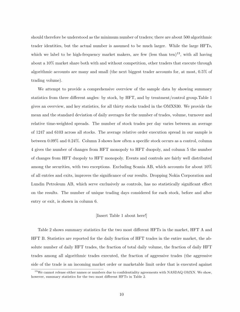
We attempt to provide a comprehensive overview of the sample data by showing summary

statistics from three different angles: by stock, by HFT, and by treatment/control group.Table 1

gives an overview, and key statistics, for all thirty stocks traded in the OMXS30. We provide the

mean and the standard deviation of daily averages for the number of trades, volume, turnover and

relative time-weighted spreads. The number of stock trades per day varies between an average

of 1247 and 6103 across all stocks. The average relative order execution spread in our sample is

between 0.09% and 0.24%. Column 3 shows how often a specific stock occurs as a control, column

4 gives the number of changes from HFT monopoly to HFT duopoly, and column 5 the number

of changes from HFT duopoly to HFT monopoly. Events and controls are fairly well distributed

among the securities, with two exceptions. Excluding Scania AB, which accounts for about 10%

of all entries and exits, improves the significance of our results. Dropping Nokia Corporation and

Lundin Petroleum AB, which serve exclusively as controls, has no statistically significant effect

on the results. The number of unique trading days considered for each stock, before and after

entry or exit, is shown in column 6.

[Insert Table 1 about here!]

Table 2 shows summary statistics for the two most different HFTs in the market, HFT A and

HFT B. Statistics are reported for the daily fraction of HFT trades in the entire market, the ab-

solute number of daily HFT trades, the fraction of total daily volume, the fraction of daily HFT

trades among all algorithmic trades executed, the fraction of aggressive trades (the aggressive

side of the trade is an incoming market order or marketable limit order that is executed against

13We cannot release either names or numbers due to confidentiality agreements with NASDAQ OMXN. We show,however, summary statistics for the two most different HFTs in Table 2.

10

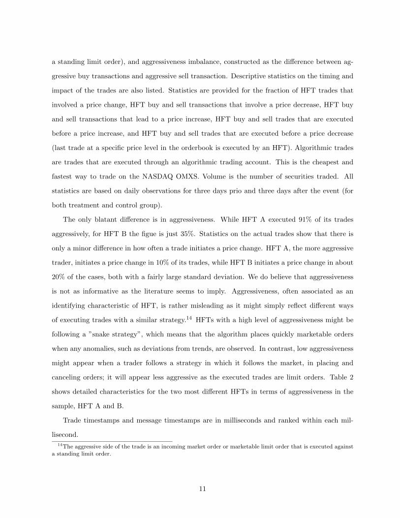
a standing limit order), and aggressiveness imbalance, constructed as the difference between ag-

gressive buy transactions and aggressive sell transaction. Descriptive statistics on the timing and

impact of the trades are also listed. Statistics are provided for the fraction of HFT trades that

involved a price change, HFT buy and sell transactions that involve a price decrease, HFT buy

and sell transactions that lead to a price increase, HFT buy and sell trades that are executed

before a price increase, and HFT buy and sell trades that are executed before a price decrease

(last trade at a specific price level in the orderbook is executed by an HFT). Algorithmic trades

are trades that are executed through an algorithmic trading account. This is the cheapest and

fastest way to trade on the NASDAQ OMXS. Volume is the number of securities traded. All

statistics are based on daily observations for three days prio and three days after the event (for

both treatment and control group).

The only blatant difference is in aggressiveness. While HFT A executed 91% of its trades

aggressively, for HFT B the figue is just 35%. Statistics on the actual trades show that there is

only a minor difference in how often a trade initiates a price change. HFT A, the more aggressive

trader, initiates a price change in 10% of its trades, while HFT B initiates a price change in about

20% of the cases, both with a fairly large standard deviation. We do believe that aggressiveness

is not as informative as the literature seems to imply. Aggressiveness, often associated as an

identifying characteristic of HFT, is rather misleading as it might simply reflect different ways

of executing trades with a similar strategy.14 HFTs with a high level of aggressiveness might be

following a ”snake strategy”, which means that the algorithm places quickly marketable orders

when any anomalies, such as deviations from trends, are observed. In contrast, low aggressiveness

might appear when a trader follows a strategy in which it follows the market, in placing and

canceling orders; it will appear less aggressive as the executed trades are limit orders. Table 2

shows detailed characteristics for the two most different HFTs in terms of aggressiveness in the

sample, HFT A and B.

Trade timestamps and message timestamps are in milliseconds and ranked within each mil-

lisecond.

14The aggressive side of the trade is an incoming market order or marketable limit order that is executed againsta standing limit order.

11


Table 3 lists descriptive statistics for all stocks and days that serve as the control group

and for all stocks and days in the treatment group. Panel A shows statistics for entries (the

change from HFT monopoly to HFT duopoly) and Panel B for exits (the change from HFT

duopoly to HFT monopoly). Order-execution time is the amount of time (in seconds) between

an incoming market order or marketable limit order and the standing limit order against which

the trade is executed. The hourly and five-minute volatilities are calculated from hourly and

five-minute intraday returns (given in squared percentages). Max-Min, Open-Close and Close-

Close volatilities are calculated as squared percentages, that is, the percentage difference squared.

Max-Min is the squared difference between the maximum price in a day and the minimum price.

Open-Close is the squared difference between the opening price and the closing price on a given

day. Close-Close is the inter-day volatility and is calculated as the squared difference between

the previous day’s closing price and today’s closing price. Further, the table shows the number

of securities traded (volume), the absolute number of daily HFT trades, the fraction of daily

HFT trades out of all algorithmic trades executed, and the daily relative time-weighted spread.

There is no significant difference between the control and treatment groups, which should not

come as a surprise given that the same stocks serve as observations in both the control and the

treatment group in relation to different stocks and different days. We isolate quite visible effects

on order-execution time and volatility after entry or exit in descriptive statistics the regressions.


5 EMPIRICAL RESULTS

Table 4 displays the estimated coefficients from our entry difference-in-differences tests of hourly

volatility computed from hourly intraday returns (column 1-4), five-minute volatility based on

five-minute intraday returns (column 5), Max-Min (column 6), Open-Close volatility (column

7) and Close-Close volatility (column 8). Besides the level variables (indicator for the treated

security and time-fixed effects), we use stock-fixed effect, volume, order execution time and lagged

12

variables as additional controls. Standard errors are clustered at the stock level and reported in

parentheses. Our findings suggest unequivocally ambiguous results on market quality. Intraday

hourly volatility increases severely by an average of over 20% and five-minute volatility by an

average of nearly 20%. Interdaily (both Open-Close and Close-Close), however, shows no sign of

any increase or decrease. These results hold for both entries and exits, noting that, for the latter,

the intraday volatility decreases (Table 5). We also provide results considering both entries and

exits as one event (one can think of exits as reverse entries) in Table 6.

[Insert Tables 4, 5, 6 about here!]

Table 7 displays the estimated coefficients from our entry difference-in-differences tests of order

execution time (columns 1-4) and the order-execution time’s daily standard deviation (column

5). Besides the level variables (indicator for the treated security and time-fixed effects), we

use stock-fixed effect, volume, volatility (computed as intraday volatility of hourly returns) and

lagged variables as controls. Standard errors are clustered at the stock level and reported in

parentheses. The order-execution time decreases on average by about 20%, which is also reflected

in a significant reduction in its standard deviation. Surprisingly, there is no significant positive

effect for exits (Table 8), only a marginally significant increase in its standard deviation. Table 9

combines entries and exits and shows marginally significant estimates.


Table 10 displays the estimated coefficients from our entry difference-in-differences tests of

volume, measured as the number of securities traded (column 1-4), and the fraction of daily

HFT volume (column 5). Besides the level variables (indicator for the treated security and time-

fixed effects), we use the stock-fixed effect, order execution time, volatility (computed as intraday

volatility of hourly returns) and lagged variables as controls. Standard errors are clustered at

the stock level and reported in parentheses. Even though the HFTs’ proportion of total volume

increases or decreases significantly after entries or exits respectively, there is, unexpectedly, no

effect on total volume. We treat this as an indication that there is a crowding-out effect, as we

13

outlined earlier in the paper.


6 CONCLUSION

High-frequency traders (HFTs) play a role of critical importance for the financial markets. We

find that competition among HFTs coincides with a stark increase in intraday volatility, but

interestingly has no effect on interday volatility. We also find a decrease in order-execution time

(the difference between an incoming market order or marketable limit order and the standing limit

order against which the trade is executed) and an increase in the market share of HFTs, although

with no effect on overall volume. We make an attempt to draw causal conclusions by exploiting

the cross-sectional variations in stocks and conducting difference-in-differences tests. This paper

provides results for both entries and exits (understood as (daily) changes from monopoly to

duopoly and vice versa), and offers several explanations in favor of our findings. To briefly sum

up the discussion, HFT competition has a stark impact on short-term volatility, as HFTs compete

for the same prices. Their investment horizon, however, is short and therefore there is no effect on

long-term volatility. There is a decrease in order-execution time, which reflects that HFT market

making responds more quickly and potentially follows a more sophisticated strategy, thereby

increasing market quality. The decrease in order-execution time, increase in the HFT market

ratio, and the seemingly steady volume suggest a crowding out of slower investors, potentially

other market makers, which become unsuccessful in placing their orders.

Through highly competitive and quick market platforms, the advantages of technologies such

as co-location and/or the use of ultra-quick algorithms, HFTs have changed and influenced finan-

cial markets substantially, taking up to 85% of today’s equity market volume. HFTs tend to end

the day with inventories that are close to zero, frequently submit and cancel limit orders and have

short holding periods. These changes have provoked intensive discussion by legislators, regulators

and investors, leading to controversial views that span topics from price manipulation, speed of

trading, and systemic risk due to a high correlation of algorithmic strategies, to price discovery

and liquidity. The quality of liquidity that HFTs potentially provide is of particular concern as

14

HFTs have replaced traditional market makers. Our findings contribute to this discussion and

give new insights into how HFTs affect markets.

Calls for more regulatory action in the HFT industry may merit a new perspective given these

new findings about the effects of competition between HFTs.

15

References

Baron, M., J. Brogaard, and A. A. Kirilenko (2012): “The Trading Profits of High Fre-

quency Traders,” Bank of Canada working paper.

Bertrand, M., E. Duflo, and S. Mullainathan (2004): “How Much Should We Trust

Differences-In-Differences Estimates?,” The Quarterly Journal of Economics, 119(1), 249–275.

Biais, B., and P. Woolley (2011): “High Frequency Trading,” .

Boehmer, Ekkehart, F. K. Y. L., and J. J. Wu (2013): “International Evidence on Algo-

rithmic Trading,” AFA 2013 San Diego Meetings Paper.

Brogaard, J., T. Hendershott, and R. Riordan (2012): “High Frequency Trading and

Price Discovery,” SSRN eLibrary.

Chau, M., and D. Vayanos (2008): “Strong-Form Efficiency with Monopolistic Insiders,” Re-

view of Financial Studies, 21(5), 2275–2306.

Clark-Joseph, A. (2012): “Exploratory Trading,” .

Cvitanic, J., and A. A. Kirilenko (2010): “High Frequency Traders and Asset Prices,” SSRN

eLibrary.

Foucault, T., S. Moinas, and B. Biais (2011): “Equilibrium High Frequency Trading,” .

Gerig, A., and D. Michayluk (2010): “Automated Liquidity Provision and the Demise of

Traditional Market Making,” .

Hagstrmer, B., and L. L. Norden (2012): “The Diversity of High Frequency Traders,” SSRN

eLibrary.

Hasbrouck, J., and G. Saar (2012): “Low-Latency Trading,” AFA 2012 Chicago Meetings

Paper.

Hendershott, T., C. M. Jones, and A. J. Menkveld (2011): “Does Algorithmic Trading

Improve Liquidity?,” The Journal of Finance, 66(1), 1–33.

16

Hendershott, T., and R. Riordan (2013): “Algorithmic Trading and the Market for Liquid-

ity,” Journal of Financial and Quantitative Analysis, forthcoming.

Hirschey, N. H. (2011): “Do High-Frequency Traders Anticipate Buying and Selling Pressure?,”

.

Huh, Y. (2013): “Machines vs. Machines: High Frequency Trading and Hard Information,” .

Jain, P. K. (2005): “Financial Market Design and the Equity Premium: Electronic versus Floor

Trading,” The Journal of Finance, 60(6), 2955–2985.

Jovanovic, B., and A. J. Menkveld (2012): “Middlemen in Limit-Order Markets,” SSRN

eLibrary.

Kirilenko, A. A., S. M. Kyle, Albert S., and T. Tuzun (2011): “The Flash Crash: The

Impact of High Frequency Trading on an Electronic Market,” SSRN eLibrary.

Li, S. (2013): “Imperfect Competition, Long Lived Private Information, and the Implications for

the Competition of High Frequency Trading,” SSRN eLibrary.

Martinez, V. H., and I. Rosu (2013): “High Frequency Traders, News and Volatility,” .

SEC, U. (2010): “Concept release on equity market structure,” concept release, 34-61358, FileNo,

17 CFR Part 242 RIN 3235–AK47.

17

A INSTITUIONAL AND MARKET BACKGROUND

The NASDAQ OMXS (Stockholm) had about an 80% market share in 2009 with the majority of

the trading volume in NASDAQ OMXS 30, listing Sweden’s largest public companies. The closest

competitor was BATS Chi-X Europe with about 10% to 15% of market share in 2009, followed

by Burgundy and Turquoise with less 5%.

The limit order book market is open Monday to Friday from 9am to 5:30pm, CET, except

red days. There is one exception though, trading closes at 1pm if the following day is a public

holiday. Both opening and closing prices are set by call auctions. Priority rank of an order during

the trading day is price, time and visibility.

To access the market, financial intermediaries have four different possibilities. (i) A broker

account, which is mostly used by institutional investors or non-automated trading. (ii) An order

routing account that allows customers of the exchange member intermediary to rout their orders

directly to the market. This is mostly used by direct banks such as internet banks. (iii) A

programmed account is typically used to execute orders through an algorithm such as a big

sequential sell or buy order. (iv) Finally, there is algorithmic trading account which is the quickest

and the cheapest in terms of transaction costs and thus a natural choice for high-frequency traders.

There are about one hundred financial firms (members) registered at NASDAQ OMXS.

An important detail about NASDAQ OMXS is that members cannot place small hidden orders.

The rule for being able to hide orders depends on the average daily turnover of a specific stock,

but must be at least 50,000EUR. This, however, increases with turnover and reaches for example

for one million euro a minimum order size of 250,000EUR. As a result, HFTs have no incentive

to hide their orders.

18

Table 1: Summary Statistics of Sample Stocks

This table presents summary statistics for the NASDAQ OMXS30 three days prior and after an entry or exit of a high-frequency market maker. It lists the ISINcode, the company’s name, number of daily trades, daily volume (in 1000 units), daily turnover (in 1000 SEK) and the relative time-weighted bid-ask spread. Column threeshows how often a specific stock occurs as a control, column four gives the number of changes from high-frequency trading (HFT) monopoly to HFT duopoly and column fivethe changes from HFT duopoly to HFT monopoly. The number of unique trading days for each stock is shown in column six (Note that a stock may serve as a control for morethan one event per day.).

ISIN Code Secuity Name Control Entry ExitCH0012221716 ABB Ltd 32 3 2FI0009000681 Nokia Corporation 48 0 0GB0009895292 AstraZeneca PLC 29 5 4SE0000101032 Atlas Copco AB A 57 2 1SE0000103814 Electrolux, AB B 79 1 1SE0000106270 Hennes & Mauritz AB, H & M B 57 4 4SE0000107419 Investor AB B 59 0 1SE0000108227 SKF, AB B 52 2 3SE0000108656 Ericsson, Telefonab. L M B 62 5 5SE0000112724 Svenska Cellulosa AB SCA B 55 1 2SE0000113250 Skanska AB B 57 2 3SE0000115446 Volvo, AB B 21 2 3SE0000122467 Atlas Copco AB B 49 2 5SE0000148884 Skandinaviska Enskilda Banken A 57 4 4SE0000163594 Securitas AB B 64 4 4SE0000171100 SSAB AB A 56 2 3SE0000193120 Svenska Handelsbanken A 46 5 5SE0000202624 Getinge AB B 60 2 3SE0000242455 Swedbank AB A 41 5 5SE0000255648 ASSA ABLOY AB B 53 3 4SE0000308280 SCANIA AB B 8 14 13SE0000310336 Swedish Match AB 32 9 8SE0000314312 Tele2 AB ser. B 54 2 2SE0000412371 Modern Times Group MTG AB B 67 5 4SE0000427361 Nordea Bank AB 47 7 6SE0000667891 Sandvik AB 50 6 5SE0000667925 TeliaSonera AB 33 5 4SE0000695876 Alfa Laval AB 35 7 7SE0000825820 Lundin Petroleum AB 74 0 0SE0000869646 Boliden AB 60 1 0

Total/Mean 1494 128 100

Trades

No Days Mean SD54 2316 107749 1545 57055 2455 86372 3331 94789 3142 131182 4236 167773 1805 51675 2798 101679 5986 201972 2266 81883 2109 81137 4171 94375 1250 46077 4651 167979 1659 78279 2746 91777 2255 96370 1535 51871 5454 207676 2270 89774 1351 63666 1446 49972 2216 85483 1485 53774 3577 138971 3406 95558 2688 139067 2215 67483 1790 51573 4241 1485

2145 2749 1648

Volume (1000)

Mean SD2829 13381205 5021321 4525224 16052701 13722060 7741924 7023082 1432

17108 87532154 8621965 9146984 21831163 510

11070 47341940 10632820 10491786 641887 473

11386 53552070 1009906 387

1012 3862001 1111355 154

9194 34475497 17689271 51832225 9621436 4815188 2019

3922 4722

Turnover (1000SEK)

Mean SD388568 176143110902 47003418987 143539488603 150242439715 223536831174 313182247540 90601350031 168788

1197412 617496208511 84315213179 99676472870 14971297269 43480

513746 211720131865 73863306488 109205338677 117238113873 58061765288 376062249035 12083582726 35999

148239 55642198433 107238110940 47783672128 260518431676 138283440023 259887193898 7989286773 28329

423193 167698

357223 324766

Bid-Ask Spread

Mean SD0.173 0.0500.112 0.0130.132 0.0580.140 0.0540.139 0.0510.093 0.0440.177 0.0530.124 0.0360.109 0.0340.118 0.0370.139 0.0450.103 0.0490.186 0.0640.169 0.0940.156 0.0500.198 0.0690.189 0.1010.169 0.0600.226 0.1400.130 0.0430.239 0.0960.143 0.0500.131 0.0160.182 0.0490.145 0.0360.133 0.0540.167 0.0750.114 0.0350.174 0.0380.156 0.071

0.153 0.070

19

Table 2: Summary Statistics of High-Frequency Traders

This table shows summary statistics for the two most different high-frequency traders in the market, high-frequencytrader A and high-frequency trader B. Statistics are reported for the daily fraction of HFT trades in the entire market,the absolute number of daily HFT trades, the fraction of total daily volume, the fraction of daily HFT trades among allalgorithmic trades executed, the fraction of aggressive trades (the aggressive side of the trade is an incoming market orderor marketable limit order that is executed against a standing limit order), and aggressiveness imbalance, constructed asthe difference between aggressive buy transactions and aggressive sell transaction. Descriptive statistics on the timing andimpact of the trades are also listed. Statistics are provided for the fraction of HFT trades that involve a price change, HFTbuy and sell transactions that involve a price decrease, HFT by and sell transactions that lead to a price increase, HFTbuy and sell trades that are executed before a price increase, and HFT buy and sell trades that are executed before a pricedecrease (last trade on a specific price level in the orderbook is executed by an HFT). Algorithmic trades are trades that areexecuted through an algorithmic trading account. This is the cheapest and fastest way to trade on the NASDAQ OMX.Volume is the number of securities traded. All statistics are based on daily observations for three days prior and after theevent (for both treatment and control group).

High-Frequency Trader AMean Median SD

HFT Trades / Total Trades 0.1001 0.0832 0.0639HFT Trades (per Day and Stock) 279 193 258HFT Volume / Total Volume 0.1033 0.0829 0.0729Closing Inventory (fraction) 0.0019 0.0000 0.0910HFT Trades / Algorithmic Trades 0.3020 0.2799 0.1528Aggressive Trades (fraction) 0.9106 0.9836 0.2345Aggressiveness Imbalance -0.0271 -0.0243 0.1538Trades Initiate a Price Changes (fraction) 0.0956 0.0710 0.0815Buy Trades Initiate a Price Decrease (fraction) 0.0117 0.0085 0.0139Sell Trades Initiate a Price Decrease (fraction) 0.0337 0.0226 0.0350Sell Trades Initiate a Price Increase (fraction) 0.0127 0.0096 0.0143Buy Trades Initiate a Price Increase (fraction) 0.0305 0.0201 0.0320Buy Trades Before a Price Decrease (fraction) 0.0402 0.0361 0.0267Sell Trades Before a Price Decrease (fraction) 0.0634 0.0584 0.0365Sell Trades Before a Price Increase (fraction) 0.0450 0.0403 0.0300Buy Trades Before a Price Increase (fraction) 0.0631 0.0588 0.0353

High-Frequency Trader BMean Median SD

0.0956 0.0757 0.0749266 190 229

0.0549 0.0379 0.04940.0024 0.0000 0.10900.2592 0.2349 0.15750.3459 0.2672 0.2123

-0.0036 0.0000 0.12950.2169 0.2018 0.16870.0625 0.0455 0.08460.0427 0.0308 0.03790.0697 0.0485 0.08970.0380 0.0291 0.03430.0471 0.0394 0.03200.0558 0.0510 0.03360.0506 0.0432 0.03510.0525 0.0460 0.0330

20

Table 3: Summary Statistics of the Control and Treatment Group

This table lists descriptive statistics for all stocks and days that serve as the control group and for all stocks andays in the treatment group. Panel A shows statistics for entries (the change from HFT monopoly to HFT duopoly) andPanel B for exits (the change from HFT duopoly to HFT monopoly). Order-execution time is the amount of time (inseconds) between an incoming market order or marketable limit order and the standing limit order against which that thetrade is executed. The hourly and five-minute volatilities are calculated from hourly and five-minute intraday returns. TheMax-Min, Open-Close and Close-Close volatilities are calculated as the sum of squared percentage changes. Max-Min is thesquared change between the maximum price within a day and the minimum price. Open-Close shows the squared changebetween the opening price and the closing price of the day. Close-Close is the inter-day volatility and calculated from thesquared change between the previous day’s closing price and today’s closing price. Further, the table shows the number ofsecurities traded (volume), the absolute number of daily HFT trades, the fraction of daily HFT trades out of algorithmictrades executed, and the daily relative time-weighted bid-ask spread. Algorithmic trades are trades that are executedthrough an algorithmic trading account. This is the cheapest and fastest way to trade on the NASDAQ OMX. All statisticsare based on daily observations.

Panel A: Entry Control GroupObs Mean Median SD

Order-Execution Time (sec) 1408 73.401 57.259 60.5555min Vola 1408 0.050 0.042 0.03360min Vola 1408 0.389 0.224 0.521Max-Min Change Squared 1358 7.302 5.206 7.208Open-Close Change Squared 1408 2.614 0.941 4.780Close-Close Change Squared 1359 3.479 1.254 7.204Volume (in 1000) 1408 3821 2182 4344HFT Volume (%) 1408 0.100 0.082 0.069Trades (#) 1408 2635 2264 1488Algorithmic Trades (#) 1408 813 698 475HFT of Algorithmic (%) 1408 0.323 0.302 0.162Bid-Ask Spread (SEK) 1408 0.161 0.143 0.066

Treatment Group Before EntryObs Mean Median SD251 60.549 53.000 58.165251 0.042 0.031 0.033249 0.281 0.196 0.311251 7.017 4.751 6.558251 3.245 1.118 4.887251 3.946 1.756 6.209251 4395 2046 6262251 0.085 0.061 0.072251 3104 2625 2041251 1021 866 639251 0.327 0.312 0.137251 0.127 0.101 0.074

Panel B: Exit Control GroupObs Mean Median SD

Order-Execution Time (sec) 1274 65.778 52.254 54.4095min Vola 1274 0.049 0.043 0.03260min Vola 1264 0.376 0.224 0.479Max-Min Change Squared 1225 7.552 5.285 7.084Open-Close Change Squared 1274 2.682 1.003 4.451Close-Close Change Squared 1225 3.306 1.208 5.675Volume (in 1000) 1274 3856 2209 4561HFT Volume (%) 1274 0.104 0.084 0.073Trades (#) 1274 2694 2309 1499Algorithmic Trades (#) 1274 858 748 465HFT of Algorithmic (%) 1274 0.325 0.310 0.152Bid-Ask Spread (SEK) 1274 0.153 0.140 0.063

Treatment Group After ExitObs Mean Median SD187 52.104 42.000 57.016187 0.037 0.029 0.031186 0.296 0.185 0.310187 6.220 3.974 6.194187 2.760 0.813 4.518187 3.884 1.625 6.679187 4669 2185 5789187 0.090 0.067 0.068187 3301 2766 2151187 1119 929 763187 0.351 0.337 0.137187 0.109 0.096 0.059

21

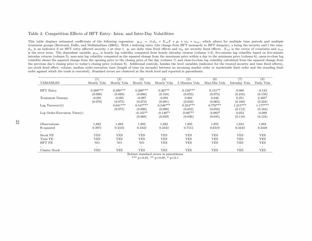
Table 4: Competition Effects of HFT Entry: Intra- and Inter-Day Volatilities

This table displays estimated coefficients of the following regression: yist = β1dis + XistΓ + pt + ms + uist, which allows for multiple time periods and multipletreatment groups (Bertrand, Duflo, and Mullainathan (2004)). With i indexing entry (the change from HFT monopoly to HFT duopoly), s being the security and t the time.dis is an indicator if an HFT entry affected security s at time t. pt are daily time fixed effects and mg are security fixed effects. Xist is the vector of covariates and uistis the error term. The dependent variable, yist, is hourly log volatility computed from hourly intraday returns (column 1-4), five-minute log volatility based on five-minuteintraday returns (column 5), max-min log volatility computed as the squared change from the maximum price within a day to the minimum price (column 6), open-to-close logvolatility shows the squared change from the opening price to the closing price of the day (column 7) and close-to-close log volatility calculated from the squared change fromthe previous day’s closing price to today’s closing price (column 8). Additional controls, besides the level variables (indicator for the treated security and time fixed effects),are stock fixed effect, volume, median order-execution time (length of time (in seconds) between an incoming market order or marketable limit order and the standing limitorder against which the trade is executed). Standard errors are clustered at the stock level and reported in parentheses.

(1) (2) (3) (4) (5) (6) (7) (8)VARIABLES Hourly Vola Hourly Vola Hourly Vola Hourly Vola 5 Minutes Vola Max-Min Vola Intraday Vola Daily Vola

HFT Entry 0.289*** 0.290*** 0.280*** 0.267** 0.150*** 0.151** 0.088 -0.123(0.090) (0.089) (0.086) (0.104) (0.053) (0.073) (0.216) (0.150)

Treatment Dummy -0.091 -0.095 -0.087 -0.091 0.004 0.046 0.251 0.405*(0.078) (0.075) (0.073) (0.081) (0.033) (0.063) (0.169) (0.224)

Log Turnover(t) 0.641*** 0.547*** 0.546*** 0.254*** 0.770*** 1.215*** 1.177***(0.075) (0.090) (0.090) (0.052) (0.059) (0.112) (0.164)

Log Order-Execution Time(t) -0.145** -0.146** 0.087** -0.082* 0.053 -0.099(0.060) (0.059) (0.036) (0.045) (0.118) (0.124)

Observations 1,882 1,882 1,882 1,882 1,905 1,855 1,834 1,804R-squared 0.3971 0.4316 0.4343 0.4343 0.7515 0.6319 0.3443 0.3448- - - - - - - - -Stock FE YES YES YES YES YES YES YES YESTime FE YES YES YES YES YES YES YES YESHFT FE NO NO NO YES YES YES YES YES- - - - - - - - -Cluster Stock YES YES YES YES YES YES YES YES

Robust standard errors in parentheses*** p<0.01, ** p<0.05, * p<0.1

22

Table 5: Competition Effects of HFT Exit: Intra- and Inter-Day Volatilities


(1) (2) (3) (4) (5) (6) (7) (8)VARIABLES Hourly Vola Hourly Vola Hourly Vola Hourly Vola 5 Minutes Vola Max-Min Vola Intraday Vola Daily Vola

HFT Exit -0.239** -0.273** -0.269** -0.254** -0.149** -0.139** -0.091 -0.002(0.114) (0.104) (0.103) (0.112) (0.070) (0.059) (0.242) (0.170)

Treatment Dummy 0.298*** 0.300*** 0.276*** 0.270*** 0.124 0.156** -0.042 0.294*(0.102) (0.092) (0.089) (0.092) (0.077) (0.073) (0.207) (0.171)

Log Turnover(t) 0.577*** 0.473*** 0.475*** 0.227*** 0.743*** 1.230*** 1.211***(0.070) (0.090) (0.090) (0.054) (0.052) (0.115) (0.155)

Log Order-Execution Time(t) -0.166** -0.164** 0.062 -0.092* -0.011 -0.114(0.062) (0.062) (0.038) (0.045) (0.106) (0.122)



23

Table 6: Competition Effects of HFT Entry and Exit: Intra- and Inter-Day Volatilities


(1) (2) (3) (4) (5) (6) (7) (8)VARIABLES Hourly Vola Hourly Vola Hourly Vola Hourly Vola 5 Minutes Vola Max-Min Vola Open-Close Vola Close-Close Vola

HFT Entry or Exit x Date (Dummy) 0.246*** 0.256*** 0.250*** 0.275*** 0.142** 0.149** 0.095 -0.030(0.082) (0.075) (0.073) (0.091) (0.053) (0.060) (0.204) (0.130)

Treatment (Dummy) -0.111 -0.144** -0.140** -0.134* 0.016 0.043 0.200 0.373(0.082) (0.069) (0.067) (0.070) (0.034) (0.063) (0.176) (0.227)

Entry or Exit 0.148* 0.160** 0.147* 0.150* -0.018 -0.023 -0.248*** 0.006(0.082) (0.076) (0.075) (0.075) (0.034) (0.064) (0.082) (0.137)

Log Turnover(t) 0.621*** 0.544*** 0.544*** 0.247*** 0.771*** 1.260*** 1.201***(0.068) (0.085) (0.085) (0.052) (0.055) (0.104) (0.160)

Log Order-Execution Time(t) -0.124** -0.122** 0.094** -0.068 0.095 -0.030(0.058) (0.057) (0.038) (0.044) (0.096) (0.119)

Passive Traders (. 50%) -0.036 -0.106* -0.111 -0.209 -0.206(0.083) (0.059) (0.079) (0.220) (0.189)



24

Table 7: Competition Effects of HFT Entry: Order-execution Time

This table displays estimated coefficients of the following regression: yist = β1dis + XistΓ + pt + ms + uist, which allows for multiple time periods and multipletreatment groups (Bertrand, Duflo, and Mullainathan (2004)). With i indexing entry (the change from HFT monopoly to HFT duopoly), s being the security and t the time.dis is an indicator if an HFT entry affected security s at time t. pt are daily time fixed effects and mg are security fixed effects. Xist is the vector of covariates and uist isthe error term. The dependent variable, yist, is log order-execution time measured by the median length of time (in seconds) between an incoming market order or marketablelimit order and the standing limit order against which the trade is executed (column 1-4) and the log order-execution time daily standard deviation (column 5). Additionalcontrols, besides the level variables (indicator for the treated security and daily time fixed effects), are stock fixed effect, volume, volatility (computed as intraday volatility ofhourly returns). Standard errors are clustered at the stock level and reported in parentheses.

(1) (2) (3) (4) (5)VARIABLES Order-Execution Time Order-Execution Time Order-Execution Time Order-Execution Time Order-Execution Time (SD)

HFT Entry -0.128** -0.124*** -0.102** -0.188*** -0.075(0.049) (0.042) (0.041) (0.056) (0.048)

Treatment Dummy 0.082 0.087 0.084 0.047 0.043(0.061) (0.056) (0.055) (0.061) (0.032)

Log Turnover(t) -0.677*** -0.642*** -0.643*** -0.161***(0.041) (0.042) (0.042) (0.026)

Log Volatility(t) -0.049*** -0.049*** 0.040***(0.010) (0.009) (0.010)

Observations 1,905 1,905 1,882 1,882 1,882R-squared 0.5938 0.6939 0.6956 0.6968 0.3637- - - - - -Stock FE YES YES YES YES YESTime FE YES YES YES YES YESHFT FE NO NO NO YES YES- - - - - -Cluster Stock YES YES YES YES YES


25

Table 8: Competition Effects of HFT Exit: Order-execution Time


(1) (2) (3) (4) (5)VARIABLES Order-Execution Time Order-Execution Time Order-Execution Time Order-Execution Time Order-Execution Time (SD)

HFT Exit 0.022 0.062 0.040 0.202*** 0.060(0.048) (0.043) (0.043) (0.054) (0.040)

Treatment Dummy -0.185** -0.196** -0.174** -0.395*** -0.068**(0.088) (0.074) (0.075) (0.082) (0.030)

Log Turnover(t) -0.668*** -0.634*** -0.635*** -0.158***(0.047) (0.047) (0.046) (0.026)

Log Volatility(t) -0.050*** -0.049*** 0.018*(0.011) (0.011) (0.009)

Observations 1,650 1,650 1,630 1,630 1,630R-squared 0.5830 0.6826 0.6844 0.6891 0.4727- - - - - -Stock FE YES YES YES YES YESTime FE YES YES YES YES YESHFT FE NO NO NO YES YES- - - - - -Cluster Stock YES YES YES YES YES


26

Table 9: Competition Effects of HFT Entry and Exit: Order-execution Time


(1) (2) (3) (4)VARIABLES Order-Execution Time Order-Execution Time Order-Execution Time Order-Execution Time

HFT Entry or Exit x Date (Dummy) -0.098* -0.102** -0.085* -0.200**(0.049) (0.043) (0.043) (0.076)

Treatment (Dummy) 0.041 0.086 0.083 -0.008(0.066) (0.060) (0.060) (0.061)

Entry or Exit -0.126* -0.155*** -0.153*** -0.116**(0.065) (0.054) (0.053) (0.052)

Log Turnover(t) -0.675*** -0.643*** -0.609***(0.041) (0.042) (0.048)

Log Volatility(t) -0.042*** -0.028**(0.010) (0.011)

Passive Traders (. 50%) 0.232**(0.106)

Observations 2,145 2,145 2,119 2,119R-squared 0.5835 0.6815 0.6825 0.7269- - - - -Stock FE YES YES YES YESTime FE YES YES YES YESHFT FE NO NO NO YES- - - - -Cluster Stock YES YES YES YES


27

Table 10: Competition Effects of HFT Entry: Trading Volume

This table displays estimated coefficients of the following regression: yist = β1dis + XistΓ + pt + ms + uist, whichallows for multiple time periods and multiple treatment groups (Bertrand, Duflo, and Mullainathan (2004)). With i indexingentry (the change from HFT monopoly to HFT duopoly), s being the security and t the time. dis is an indicator if an HFTentry affected security s at time t. pt are daily time fixed effects and mg are security fixed effects. Xist is the vector ofcovariates and uist is the error term. The dependent variable, yist, is log volume measured as daily turnover (column 1-4)and the fraction of daily HFT volume (column 5). Additional controls, besides the level variables (indicator for the treatedsecurity and time fixed effects), are stock fixed effect, order-execution time (length of time (in seconds) between an incomingmarket order or marketable limit order and the standing limit order against which the trade is executed) volatility (computedas intraday volatility of hourly returns). Standard errors are clustered at the stock level and reported in parentheses.

(1) (2) (3) (4)VARIABLES Daily Volume Daily Volume Daily Volume Daily HFT Volume

HFT Entry -0.005 -0.040 -0.012 0.078***(0.034) (0.029) (0.034) (0.011)

Treatment Dummy 0.007 0.028 0.012 0.002(0.038) (0.034) (0.033) (0.006)

Log Order-Execution Time(t) -0.319*** -0.321*** -0.026***(0.031) (0.032) (0.004)

Log Volatility(t) 0.061*** 0.061*** -0.004***(0.012) (0.012) (0.001)

Observations 1,905 1,882 1,882 1,882R-squared 0.8420 0.8803 0.8805 0.6438- - - - -Stock FE YES YES YES YESTime FE YES YES YES YESHFT FE NO NO YES YES- - - - -Cluster Stock YES YES YES YES


Table 11: Competition Effects of HFT Exit: Trading Volume


(1) (2) (3) (4)VARIABLES Daily Volume Daily Volume Daily Volume Daily HFT Volume

HFT Exit 0.068* 0.069** 0.033 -0.078***(0.038) (0.032) (0.045) (0.012)

Treatment Dummy -0.012 -0.067 -0.053 0.081***(0.052) (0.040) (0.043) (0.015)

Log Order-Execution Time(t) -0.319*** -0.324*** -0.025***(0.038) (0.039) (0.004)

Log Volatility(t) 0.056*** 0.056*** -0.004**(0.013) (0.013) (0.001)

Observations 1,650 1,630 1,630 1,630R-squared 0.8455 0.8810 0.8815 0.6567- - - - -Stock FE YES YES YES YESTime FE YES YES YES YESHFT FE NO NO YES YES- - - - -Cluster Stock YES YES YES YES


28

Table 12: Competition Effects of HFT Entry and Exit: Trading Volume


(1) (2) (3)VARIABLES Daily Volume Daily Volume Daily HFT Volume

HFT Entry or Exit x Date (Dummy) -0.023 -0.020 0.077***(0.034) (0.038) (0.011)

Treatment (Dummy) 0.059 0.048 0.000(0.043) (0.037) (0.005)

Entry or Exit -0.029 -0.063** -0.001(0.036) (0.027) (0.005)

Log Order-Execution Time(t) -0.305*** -0.027***(0.031) (0.004)

Log Volatility(t) 0.063*** -0.005***(0.012) (0.001)

Passive Traders (. 50%) -0.043***(0.014)

Observations 2,145 2,119 2,119R-squared 0.8442 0.8796 0.6470- - - -Stock FE YES YES YESTime FE YES YES YESHFT FE NO YES YES- - - -Cluster Stock YES YES YES


29

Figure 1: Stylized Motivating Example: Participation

This figure presents a motivating example how entry (the change from monopoly to duopoly) of a high-frequencymarket maker typically affects trading participation within an average stock. It shows the incumbent high-frequency trader(HFT) and the entering HFT. Daily ratios of both HFTs’ trading participation and total stock turnover are plotted.

050

010

0015

0020

0025

00T

urno

ver

(mill

ion

SE

K)

05

1015

2025

Dai

ly T

rade

Par

ticip

atio

n (%

)

t t+30 t+60 t+90 t+120 t+150 t+180Date (Days)

Incumbent HFT Entering HFT

Daily Total Turnover

30

Figure 2: Stylized Motivating Example: Inventory

This figure shows a motivating example of an entering high-frequency market maker. It present high-frequencytrading inventory over a period of 20 days. Each vertical line represents the beginning of a new trading day. The gray areais one entry event that enters the analysis. While the lighter gray area are trading days of the incumbent alone, the darkergray area are days facing competition.

-50

510

Inve

ntor

y (m

illio

n S

EK

)

t t+2 t+4 t+6 t+8 t+10 t+12 t+14 t+16 t+18 t+20Trading Days

Figure 3: Entries and Exits over Time

All entries and exits that occur during the transition period from a single high-frequency market maker to competi-tion are pictured in this figure. Each tick on the y-axis is one of the 30 individual stocks.

05

1015

2025

30In

divi

dual

Sto

cks

(OM

XS

30)

t t+30 t+60 t+90 t+120 t+150 t+180 t+210Date (Days)

HFT Entry HFT Exit

31

Figure 4: Summary Statistics of High-Frequency Trading Participation

This figure shows graphically average deviations from average trading participations of individual stocks for both the control and the treatment group. Average trad-ing participation under no competition is about 10%. The left-hand-side of the graph shows average effects of entries and the right-hand-side average effects of exits three daysprior and three days after the event.

-.2

0.2

.4.6

.8H

FT

Par

ticip

atio

n (%

)

-3 -2 -1 0 1 2Distance to Event (Days)

Treatment Control

Entry

-.2

0.2

.4.6

.8H

FT

Par

ticip

atio

n (%

)


Treatment Control

Exit

32

Figure 5: Summary Statistics of Short-Term Volatility

This figure illustrates average deviations from average short-term volatilities (60 minute volatilities) of individual stocks for both the control and the treatmentgroup. The left-hand-side of the graph shows average effects of entries and the right-hand-side average effects of exits three days prior and three days after the event.

-.2

0.2

.4V

olat

ility

(%

)


Treatment Control

Entry

-.2

0.2

.4V

olat

ility

(%

)


Treatment Control

Exit

33

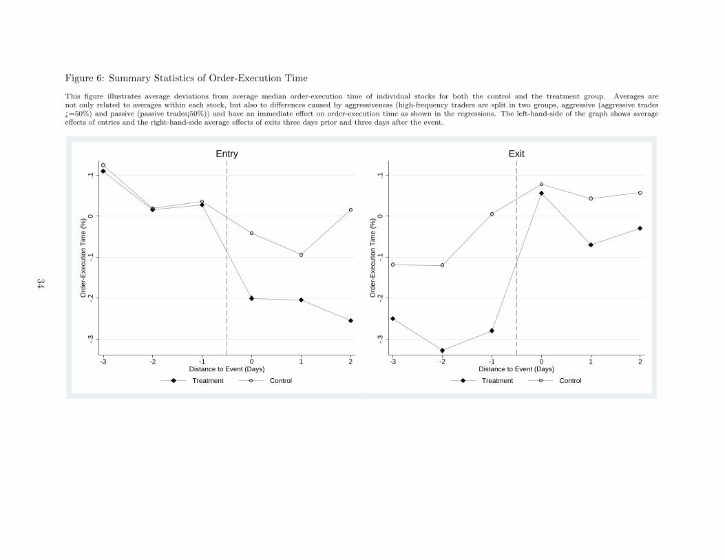
Figure 6: Summary Statistics of Order-Execution Time

This figure illustrates average deviations from average median order-execution time of individual stocks for both the control and the treatment group. Averages arenot only related to averages within each stock, but also to differences caused by aggressiveness (high-frequency traders are split in two groups, aggressive (aggressive trades¿=50%) and passive (passive trades¡50%)) and have an immediate effect on order-execution time as shown in the regressions. The left-hand-side of the graph shows averageeffects of entries and the right-hand-side average effects of exits three days prior and three days after the event.

-.3

-.2

-.1

0.1

Ord

er-E

xecu

tion

Tim

e (%

)


Treatment Control

Entry

-.3

-.2

-.1

0.1

Ord

er-E

xecu

tion

Tim

e (%

)


Treatment Control

Exit

34

Figure 7: Intraday Average Inventory of High-Frequency Traders

This figure pictures the average intraday inventory over all stocks and days for five minute bins. Inventory is de-fined as the cumulative turnover divided by total turnover within each five minute bucket. While the left graph views averageinventory over all days and stocks with a monopolistic high-frequency trader, the right hand graph shows inventories undercompetition for both the incumbent and entrant. Trading takes place from 9am to 5:30pm.

-1-.

50

.51

Inve

ntor

y (f

ract

ion)

9:00 10:30 12:00 1:30 3:00 4:30 5:30Time (5 minute steps)

Monopolist (Median) Monopolist (Mean)

-1-.

50

.51

Inve

ntor

y (f

ract

ion)

9:00 10:30 12:00 1:30 3:00 4:30 5:30Time (5 minute steps)

Incumbent (Median) Entrant (Median)

Entrant (Mean) Incumbent (Mean)

35

Figure 8: Competition over the Same Trades

This figure images the average intraday fraction of trades that were executed on the same side of the market (overall stocks and days) for five minute and sixty minute bins under competition. Trades are executed on the same side of themarket if within each bin both the entrant and the incumbent buy or sell. The measure is constructed by assigning one ifboth high-frequency traders trade on the same side of the market and zero if not. The average ratio of trading on the sameside of the market as their competitor is 2/3. The dark shaded bars are hourly averages. The market is open from 9am to5:30pm.

.5.6

.7.8

.9F

ract

ion

of B

eing

on

the

Buy

/Sel

l Sid

e

9:00 10:30 12:00 1:30 3:00 4:30 5:30Time

36

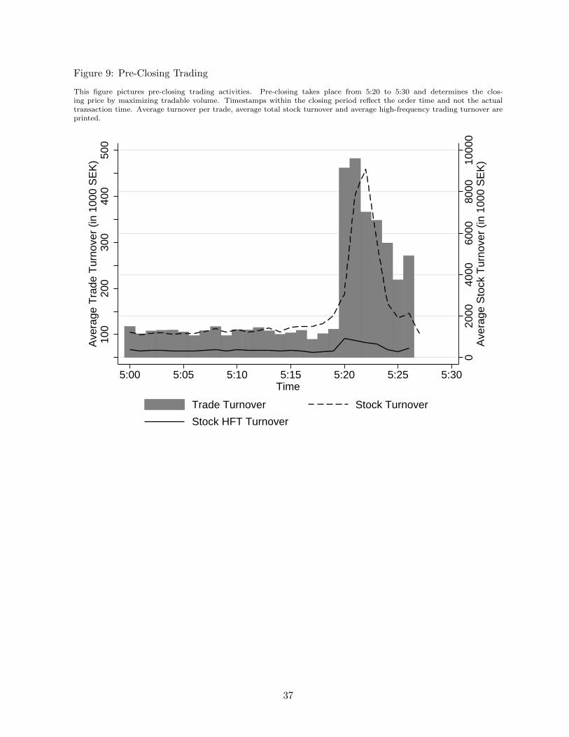
Figure 9: Pre-Closing Trading

This figure pictures pre-closing trading activities. Pre-closing takes place from 5:20 to 5:30 and determines the clos-ing price by maximizing tradable volume. Timestamps within the closing period reflect the order time and not the actualtransaction time. Average turnover per trade, average total stock turnover and average high-frequency trading turnover areprinted.

020

0040

0060

0080

0010

000

Ave

rage

Sto

ck T

urno

ver

(in 1

000

SE

K)

100

200

300

400

500

Ave

rage

Tra

de T

urno

ver

(in 1

000

SE

K)

5:00 5:05 5:10 5:15 5:20 5:25 5:30Time

Trade Turnover Stock Turnover

Stock HFT Turnover

37

Figure 10: Dynamic Impact of Entry and Exit on Volatility

This figure shows point estimates for three days before and three days after the event from the difference-in-differences estimation. We consider five days before andfive days after the event. The plotted coefficients originate from following regression:

yist = β1d−5is + β2d

−4is + · · ·+ β10d

5is +XistΓ + pt +ms + uist,

which allows for multiple time periods and multiple treatment groups (Bertrand, Duflo, and Mullainathan (2004)). With i indexing entry (the change from HFT monopoly to

HFT duopoly and vice versa), s being the security and t the time. djis is an indicator for the distance, j, if an HFT entry or exit affected security s at time t. pt are daily timefixed effects and mg are security fixed effects. Xist is the vector of covariates and uist is the error term. The dependent variable, yist, is hourly volatility computed from hourlyintraday returns. On the left, we show the volatility increase after entry and on the right we show the volatility decrease after exit.

-.4

-.2

0.2

.4.6

Vol

atili

ty (

%)


Entry

-.4

-.2

0.2

.4.6

Vol

atili

ty (

%)


Exit

38

Figure 11: Dynamic Impact of Entry and Exit on Order-execution Time

This figure shows point estimates for three days before and three days after the event from the difference-in-differences estimation. We consider five days before andfive days after the event. The plotted coefficients originate from following regression:

yist = β1d−5is + β2d

−4is + · · ·+ β10d

5is +XistΓ + pt +ms + uist,

which allows for multiple time periods and multiple treatment groups (Bertrand, Duflo, and Mullainathan (2004)). With i indexing entry (the change from HFT monopoly to

HFT duopoly and vice versa), s being the security and t the time. djis is an indicator for the distance, j, if an HFT entry or exit affected security s at time t. pt are daily timefixed effects and mg are security fixed effects. Xist is the vector of covariates and uist is the error term. The dependent variable, yist, is hourly volatility computed from hourlyintraday returns. On the left, we show the median order-execution time decrease after entry and on the right we show the median order-execution time increase after exit.

-.6

-.4

-.2

0.2

Ord

er-E

xecu

tion

Tim

e(%

)


Entry

-.6

-.4

-.2

0.2

Ord

er E

xecu

tion

Tim

e (%

)


Exit

39

competition of high-frequency market makers and market quality

Documents