Competition in Corruptible Markets

Shubhranshu Singh∗

September 2012

Preliminary

Abstract

Emerging markets offer significant business opportunities. However, local and foreign

firms selling in these markets are often faced with corrupt agents. This paper investigates

the marketing strategy implications for firms competing for business in a corruptible mar-

ket. I consider a setting in which a buyer (a firm or government) seeks to purchase a good

through a corruptible agent. Supplier firms, that may or may not be a good fit, compete to

be selected by the agent. Only the agent observes whether or not a firm is a good fit. Cor-

ruption arises due to incentive of the agent to select a non-deserving firm in exchange for

bribes. Intuitively and as expected, a sufficiently large monitoring of the agent eradicates

corruption. But the interesting point is that increasing the monitoring from an initial low

level can backfire, making the agent more likely to select a non-deserving firm. As firms

become reluctant to offer bribes in response to higher monitoring, it now becomes likely

that the agent receives a bribe offer, in equilibrium, only from a non-deserving firm. This

non-monotonic agent behavior makes it difficult to reduce corruption. The implication is

that the buyer should choose either to be ignorant or to take drastic measures to limit

corruption. Further, I show that unilateral anti-corruption controls, such as the Foreign

Corrupt Practices Act of 1977, on a U.S. firm seeking business in a corrupt foreign market

can actually increase the profits of the U.S. firm. This is because such a control on the U.S.

firm puts pressure on the buyer to set monitoring at higher levels and reduces corruption.∗I am indebted to Pedro Gardete, Ganesh Iyer, Przemyslaw Jeziorski, Shachar Kariv, Zsolt Katona, Minjung

Park and Miguel Villas-Boas for their guidance and comments. Any errors are my own. This is a preliminarydraft; comments are appreciated. Correspondence: Walter A. Haas School of Business, University of Californiaat Berkeley, Berkeley, CA 94720, USA. Email: shubhranshu_singh@haas.berkeley.edu.

1 Introduction

1.1 Overview

While the GDP growth in the more developed countries remains sluggish emerging economiesare forecasted to continue growing at rates over 6%, as per IMF estimates. Increased purchasing-power of the sizable middle class consumers and public investments in infrastructure and defensein emerging markets has created significant business opportunities for domestic as well as foreignfirms. U.S. firms, facing saturation in domestic markets, are increasingly counting on consumers,firms and governments in emerging markets as a source of future growth.1 One of the biggestchallenges faced by U.S. firms competing for business in emerging markets is corruption.2 Briberyin the emerging economies is considered a norm. Although more prevalent, corruption is by nomeans limited to emerging economies. We study competition in corruptible markets. Thefollowing examples illustrate the general framework that we have in mind.

DaimlerChrysler AG, between 1998 and 2008, paid at least $56 million in improper paymentsto government officials in China, Russia, Indonesia and other countries. The company earned$1.9 billion in revenue and at least $90 million in illegal profits through these tainted sales trans-actions. Daimler paid $185 million in fines to settle charges with the Securities and ExchangeCommission (SEC) and the U.S. Department of Justice.3

BP, like other large oil companies, charters oil tankers from shipping firms (such as Maerskand Frontline). Tanker chartering is an area that requires specialized skills and knowledge. LarsDencker Nielsen, a senior executive in BP’s tanker chartering division, allegedly received cashpayments from a shipping magnate in return for giving multimillion pound contracts over aperiod of five years.4 Bribery of private sector employees is illegal according to the Bribery Act2010 in the UK.

Bofors AB of Sweden was selected by Indian government to supply over 400 Howitzer fieldguns in a $285 million procurement decision in March 1986. It is speculated that Bofors paid

1Foreign profits as a share of global profits for U.S. firms has increased from 21% in 2000 to 46% in 2010.(Sources: S&P 500: 2010 Global Sales report and U.S. Bureau of economic analysis)

2Transparency International’s Perception of Corruption Index (2011) for major developing economies: Brazil3.8, China 3.6, India 3.1, Mexico 3.0, Indonesia 3.0 and Russia 2.4.

3http://www.sec.gov/news/press/2010/2010-51.htm; Accessed 07/31/124http://www.telegraph.co.uk/finance/newsbysector/energy/oilandgas/9144236/BP-alerted-to-bribery-at-its-

tanker-division.html; Accessed 06/15/12

2

$11.5 million in kickbacks to top Indian politicians and key defense officials to beat its competitorSofma, France and secure the deal.5 The guns were used extensively in the Kargil War betweenIndia and Pakistan in 1999 at elevations of 16000-18000 ft. The Indian army pushed the gunsbeyond their prescribed limits and used them in ways never before employed by the SwedishArmy or Bofors. The guns gave India ‘an edge’ over Pakistan according to Indian Army officersin the field.6

There are some features, in the above examples, that we would like to highlight. The decisionto select one firm over another is usually not straightforward. The selection of a firm that is bestsuited for a particular project requires expertise in the subject matter and information about theenvironment in which the product is to be used. The suppliers themselves may not know if theyare best suited. The buyers, firms or governments, rely on agents such as experts or bureaucratsto make the selection decision on their behalf. This creates the scope of corruption. The agents,sometimes but not always, select a non-deserving firm in exchange for bribes. Buyers understandan agent’s incentives to select a non-deserving firm. Corrupt agents sometimes get caught andpunished. We capture these features in our model.

We analyze the firm’s incentives for bribing an agent who selects, on the behalf of the buyer,a deserving firm from two firms that are competing for a project. Only the agent knows if aparticular firm is deserving or not. The agent is willing to select a non-deserving firm in theexchange for a bribe. We refer to the selection of a non-deserving firm as a dishonest agentbehavior. A dishonest agent behavior hurts the buyer. The buyer understands an agent’sincentives and randomly monitors the agent. Monitoring the agent is costly. Upon monitoring,the buyer learns if a non-deserving firm was selected. A dishonest agent, if caught, is punished.Firms compete in bribes to get selected by the agent. A sufficiently large monitoring eradicatescorruption as firms find it unprofitable to offer large bribes that must be offered to compensatethe agent’s higher expected penalty. For any smaller monitoring corruption prevails. The bribeoffer equilibrium is in mixed strategies. The profits of firms increase in the monitoring. Thishappens because when firms are required to pay higher bribes to be selected with certainty theybecome less willing to do so. The equilibrium bribes decrease and result in higher profits for thefirms.

5http://indiatoday.intoday.in/story/Key+players+in+Bofors+scandal/1/39264.html; Accessed 06/15/126http://www.ndtv.com/article/india/why-the-army-loves-the-bofors-gun-5580; Accessed 09/05/12

3

We also find that an increase in monitoring does not always result in more honest agentbehavior. Interestingly, if bribery is prevalent, a small increase in the monitoring can makethe agent more dishonest. The intuition is the following. If monitoring is small both firmsoffer bribes with probability one. The agent in this case often accepts the bribe offer of thedeserving firm. If monitoring is increased firms become less likely to offer bribes. The agent isnow faced with situations in which she receives a bribe offer only from a non-deserving firm. Thisforces the agent to select a bribe-offering, non-deserving firm more often. The agent becomesmore dishonest as a result of higher monitoring. If the monitoring is sufficiently large theagent always selects the deserving firm. Various scholars have discussed this non-monotonicrelationship between monitoring, or expected penalty, and honest behavior (see Akerlof andDickens (1982) and Bénabou and Tirole (2006)). However, they draw upon the classic work onintrinsic motivation in psychology (see Deci (1972)). We present a rational agent model withno behavioral assumptions and show that an increase in monitoring can make the agent moredishonest. In our model, endogenous firm response to an increase in the monitoring makes theagent more dishonest.

The non-monotonic effect of the monitoring on the agent behavior makes it difficult for thebuyer to reduce corruption. We find that, the buyer should either choose to be ignorant aboutcorruption or commit to take drastic measures to limit it. A small monitoring only hurts thebuyer.

Bribery of foreign government officials by U.S. firms competing in overseas markets wascommonplace. During an investigation by the U.S. Securities and Exchange Commission, inmid-1970s, more than 400 U.S. companies admitted to having made questionable payments toforeign government officials. Congress enacted the Foreign Corrupt Practices Act (FCPA) of1977 to bring a halt to the bribery of foreign officials and to restore public confidence in theintegrity of the American business system.7 This unilateral control on the U.S. firms seekingbusiness in foreign markets has been a topic of debate. In the business community it is believedthat the Act puts American businesses at a competitive disadvantage in international business(see Kaikati and Label (1980) for a discussion). The evidence from a majority of empiricalstudies suggests that there is little or no disadvantage posed by the FCPA (see Graham (1984),Beck, Maher, and Tschoegl (1991), and Wei (2000)). On the contrary, James R. Hines (1995)

7See www.justice.gov/criminal/fraud/fcpa/ (accessed 6/19/12) for the history and details of the Act.

4

suggests that the FCPA serves to weaken the competitive position of the U.S. firms.We study the effect of a unilateral anti-corruption control, such as the FCPA, on a firm’s

profits. We show that the profits of the controlled U.S. firm can actually increase as a resultof a unilateral anti-corruption control on it. The intuition is the following. A unilateral anti-corruption control on a firm reduces the bribe that the other firm must pay in order to getselected by the agent regardless of whether it is deserving or not. As a result, the agent selectsa non-deserving firm with a higher probability. This hurts the buyer. The buyer may, therefore,strategically, set a higher monitoring to discourage bribery by the firm that is not controlled.Since higher monitoring results in higher profits for both firms, a unilateral control can lead tohigher profits for the controlled firm. There is evidence of higher monitoring in the Middle Eastin the post-FCPA era presented in Gillespie (1987). She also concludes that the potential of theFCPA to hurt U.S. exports remains unproven.

1.2 Related Literature

Corruption has been studied extensively in many different contexts in the literature (See Jain(2001) for a review). Shleifer and Vishny (1993) study the implications of the structure ofthe corruption network on the level of corruption in government agencies. Mookherjee andPng (1995) study the optimal compensation policy for a corruptible inspector, charged withmonitoring pollution from a factory. Hauser, Simester, and Wernerfelt (1997) look at bribery,or side payments, in the context of ratings given by salesforce to internal sales support.

There is relatively smaller literature on competition in the presence of corruption. Rose-Ackerman (1975) initiate this work by presenting a model in which corruption results in alloca-tive inefficiency. The inefficiency in her model arises due to differences in the bribing capacityof competing firms or due to vague preferences of the government. Burguet and Che (2004)allow the agent to manipulate her quality evaluations in exchange for bribes. They find thatif the agent has little manipulation power, corruption does not disrupt allocation efficiencybut makes the efficient firm compete more aggressively. However, if the agent has substantialmanipulation power, corruption facilitates collusion among competing firms and creates alloca-tive inefficiency as bribery makes it costly for the efficient firm to secure a sure win. Compte,Lambert-Mogiliansky, and Verdier (2005) incorporate corruption in procurement auction through

5

the possibility for bid readjustment that an agent may provide in exchange for a bribe. Theyshow that corruption facilitates collusion in price between firms and results in a price increasethat goes beyond the bribe received by the bureaucrat. They also show that a unilateral anti-corruption controls on an efficient firm may restore price competition to some extent. Brancoand Villas-Boas (2012) investigate the effect of the degree of competition on corruption in thecontext of a firm’s investment in behaving according to the rules of the market.

This paper also relates to literature on strategic information transmission in the presenceof a third party. Scharfstein and Stein (1990) examine behavior of an advisor who cares abouthis reputation for accuracy and show that advisor’s incentive to say the expected thing canresult in herd behavior. Durbin and Iyer (2009) study information transmission to a decisionmaker from an advisor that values his reputation for incorruptibility in the presence of a thirdparty who offers unobservable bribes to influence the advice. They show that the advisor maysend an inaccurate message in order to bolster his reputation for incorruptibility. Inderst andOttaviani (2012) present a model of competition in which product providers compete to influenceintermediaries’ advice to consumers through hidden kickbacks or disclosed commissions. Theystudy equilibrium commissions and welfare implications of commonly adopted policies such asmandatory disclosure and caps on commissions.

This work contributes to the literature on competition in the presence of corruption bypresenting a model which captures the roles of corruption. Unlike Rose-Ackerman (1975), weassume firms to be symmetric and the government preference to be well defined. The scope ofcorruption arises as the buyer does not have the expertise or the information needed to makethe purchase decision and delegates the decision to an agent. Compte, Lambert-Mogiliansky,and Verdier (2005) exogenously impose corruption. The buyer does not need an agent in theirsetup. Corruption arises endogenously in our setup, more like Burguet and Che (2004). Theexisting papers do not explicitly model both the agent and the buyer. Our agent is strategic. Sheunderstands the implications of dishonest behavior and does not always accept the higher bribe.The buyer is also strategic. She understands the incentives of the agent and tries to discipline her.By accommodating these features, which have been largely ignored in the existing literature, weare able to gain interesting new insights on competition in the presence of corruption. We showthat an agent can become more dishonest as a result of increased monitoring using a rationalagent model. We also provide a formal explanation for the disconnect between the common

6

perception of the impact of the FCPA on the U.S. firms and the findings of the empirical studies.The findings of our work have important implications for firms doing business in internationalmarkets as well as governments.

The rest of the paper is organized as follows. The next section presents the model wherewe discuss firms’ decisions, agent’s decision and buyer’s decision in order. In Section 3 theanalysis of the unilateral control setup and its comparison to the model discussed in Section 2is presented. Section 4 summarizes our results.

2 Model

Consider a buyer that needs to buy a single, indivisible good. The suppliers of the product canbe one of the two possible types, good fit or bad fit. Utility of the buyer who buys the productat price p is given by V (vf , p) = vf − p, where vf = v if the product is bought from a supplierwith good product fit and vf = 0 if it is bought from a supplier with bad product fit. The buyerdoes not have the expertise or the information needed to evaluate the product fit. Therefore,firms are identical to the buyer. The reservation price of the buyer p̄.

Two firms, i = 1, 2, compete to supply the product to the buyer. One of the two firm’sproduct is a good fit, the other’s product is a bad fit. The probability that firm i’s product isa good fit is 0.5. Firms do not know if their product is a good fit or not. This may happenbecause firms may not be aware of the intended use of the good, previous training received bybuyer’s staff, and the environment in which the good will be used or due to the firm’s own lackof prior experience. Both firms have same cost of production which is assumed to be zero.

An agent, such as a bureaucrat, selects one of the two firms on behalf of the buyer. Theagent, costlessly and privately, learns the fit of the firm. This learning, while informative, is notperfect. The probability that a firm is actually a fit, given the agent’s signal is fit, is ρ > 0.5.The agent is expected to always select the firm for which she receives a fit signal. The agent, inexchange for a bribe bi ≥ 0 (bj ≥ 0) from firm i (firm j 6= i), can change her report and selecta firm that she believes is misfit. Both firms simultaneously and privately submit price bids piand pj, and bribe offers bi and bj to the agent. Price bids are observed by the buyer. From hereonwards, we refer to the firm, for which the agent receives a fit signal, as the deserving firm andthe other firm as the non-deserving firm. The agent receives the bribe conditional on the firm

7

receiving the order to supply the product. The buyer understands that the agent may accept thebribe and select a non-deserving firm. In order to discourage the agent from this behavior, thebuyer monitors the agent with probability λ ∈ [0, 1] after the good is purchased.8 The cost ofthe monitoring c (λ) is assumed to be continuous and strictly convex with c (0) = 0. The buyer,as a result of monitoring, learns the signal that agent received and infers if the agent made adishonest decision in exchange for a bribe. The buyer does not observe the bribe transfer. Thisis because in most cases no official record of the bribe transfer exists.9 In cases where a recorddoes exist the buyer may not have access to those records.10 A penalty P is imposed on thedishonest agent. We assume that P > p̄/2.11 All parties are risk neutral. The expected penaltyimposed on the agent, if she makes a decision inconsistent with her signal, is simply λP . Theminimum bribe needed in order for the agent to select a non-deserving firm, therefore, is λP .

Now we look at the agent’s incentives in the selection process. The agent compares the twobribe offers bi and bj. If | bi − bj |> λP , she selects and accepts the bribe from the firm whichmade the high bribe offer regardless of whether the firm is deserving or not. The agent, in thiscase, pays an expected penalty of λP

2 . If, however, | bi − bj |≤ λP she selects the deservingfirm and receives the bribe offered by that firm, even if it is lower than the bribe offered by theother firm. The agent, acting honestly for buyer, does not pay any penalty in this case. Here,the agent does not accept the non-deserving firm’s bribe offer because the cost of doing so inthe form of expected penalty (λP ) is weakly higher than the benefit (a bribe higher by ≤ λP ).We assume that the agent makes an honest decision if she is indifferent to either selecting thedeserving or the non-deserving firm. The payoff function of the agent can, therefore, be writtenas

πa (bi, bj) =

max(bi, bj)− λP

2 if |bi − bj| > λP

bdes if |bi − bj| ≤ λP

8In our model monitoring captures many different things. It captures the efficiency of the legal system,extent of whistle-blower protection, and extent of control on media apart from the probability with which somedepartment or agency verifies the selection decision of the agent.

9Bribes are typically paid in cash or as non-monetary benefits. Also, they are often transferred to foreignbank accounts of the agent or are received by relatives of the agent.

10Many foreign banks typically do not disclose information about their clients’ accounts to the governments.According to different estimates Indians have $500 billion to $1.5 trillion of illegal money stashed in foreign banks.According to a Global Financial Integrity report China tops the list of highest illicit financial flows (2002-2006)from developing countries accompanied by Russia, India and Indonesia in the top 10 among others.

11This assumption ensures that the buyer can make the agent honest with probability one by making λsufficiently large.

8

where, bdes is the bribe offered by the deserving firm.A particular firm gets selected by the agent with probability one (zero) if its bribe offer is

higher (lower) than the bribe offer of the other firm by more than λP . If the difference in bribesoffered is weakly less than λP the agent selects the firm only with probability 0.5, when it is adeserving firm. The expected profit of the firm i as a function of the bribes offered by firm i andfirm j 6= i can be written as

πi (bi, bj) =

pi − bi if bi > bj + λP

12 (pi − bi) if bj − λP ≤ bi ≤ bj + λP

0 if bi < bj − λP

Figure 1 summarizes the timing of the actions. In the first stage, nature makes a draw ofthe fit, from a distribution that is common knowledge, and assigns it to firms. The buyer thensets the probability with which the agent will be monitored after making the firm selection.Firms then submit simultaneous price and bribe bids to the agent. Next, the agent comparesthe bids and selects one of the two firms. The selected firm receives the accepted price anddelivers the good to the buyer. In the next stage, the buyer randomly monitors the agent andimposes a penalty if a dishonest behavior is inferred. Finally, payoffs are realized. We look forNash equilibrium in pure as well as mixed strategies. The computation of the mixed strategyequilibrium is similar to that of Varian (1980) and Narasimhan (1988).

nature draws fit andassigns it to firms

firms submit price bidsand bribe offers payoffs are realized

buyer setsmonitoringfrequency

agent selects one of the twofirms and buyer randomly

monitorsFigure 1: Timing

The framework described above has two important features that are missing in the existingliterature on competition in presence of corruption. First, our agent is strategic. She doesnot always accept the higher bribe. Also, she does not always change her report when sheaccepts a bribe. There are implications for a dishonest behavior and the agent takes them into

9

account. The buyer is also strategic. She understands the incentives of the agent to cheat.There are, therefore, consequences for dishonest agent behavior. The buyer, in equilibrium, setsa monitoring which maximizes her payoffs.

2.1 Price and Bribe Decisions

In this section the stages of the model that are relevant for the price and the bribe offer decisionsof firms are described. A firm is selected by the agent either because it is deserving or becauseit offers a sufficiently large bribe. The agent can classify a non-deserving firm as a deservingfirm.12 Given this power of the agent, a firm can always benefit by increasing the price bid solong as the price is not rejected by the buyer. Both firms, therefore, submit price p̄ as theirprice bid and compete in bribes to be selected by the agent. This leads us to the following result:

Lemma 1 Both firms submit buyer’s reservation price p̄ as their price bid.

This high price bid is a typical result in the literature and has been interpreted as corruptionfacilitating collusion (see Compte, Lambert-Mogiliansky, and Verdier (2005)).

Firm i, when confronted with a bribe offer bj of the firm j, responds by making a bribe offerthat can have three different implications. First, it can offer a bribe which is higher than bj

by more than λP and be selected with probability one. Second, it can offer a bribe which isdifferent from bj by, at-most, λP and be selected only if it is deserving. Lastly, it can offer abribe which is lower than bj by more than λP and be selected with probability zero. However,we note that:

Lemma 2 Firm i responds to a bribe offer bj of firm j by offering a bribebi ∈ {bj + λP,max (0, bj − λP )}.

The intuition for this result is as follows. Any offer bi > bj + λP is strictly dominated by anoffer bi− ε for small enough ε. Firm i still gets selected with probability one but offers a smallerbribe. Any bribe offer by firm i such that bj + λP ≥ bi > bj − λP is strictly dominated by the

12This is consistent with general observation about the discretionary power of agents in corrupt countries. (Seeanti-corruption profiles for various countries at www.trust.org/trustlaw for detailed information.)

10

offer bj − λP as firm i still gets selected whenever it deserves but pays a smaller bribe. We donot consider negative bribes, as they are never accepted. Firm i, therefore, responds to bribeoffer bj by offering one of the two bribes as specified in Lemma 2.

Now we look at the equilibrium in bribes (proofs are in the Appendix).

Proposition 1 If λ ≥ p̄2P in equilibrium both firms offer no bribes and the agent selects the

firm that is deserving. If λ < p̄2P there is no Nash equilibrium in pure strategies.

The intuition behind this proposition is the following. Higher monitoring leads to higherexpected penalty for the agent. A higher bribe, therefore, must be offered if a firm expects tobe chosen even when it is non-deserving. A deviating firm’s profits decrease with an increase inthe monitoring. For sufficiently large monitoring (λ ≥ p̄

2P ), gains from deviations are completelyerased. In this region, a pure strategy Nash equilibrium exists and firms offer no bribes inequilibrium. Since firms offer no bribes and are selected when they are deserving the equilibriumprofit for both firms is p̄

2 . This profit does not depend on the monitoring chosen by the buyerso long as it is larger than p̄

2P .If the monitoring is lower (λ < p̄

2P ), the equilibrium bribe offers are in mixed strategies.Firms respond to the other firm’s bribe offer either by offering a higher bribe just enough tosecure a sure win or by offering a lower bribe just enough to have the firm selected whenever itis deserving. The best response for a firm changes from a higher bribe offer to a lower bribe offerwhen the bribe offer of the other firm becomes high enough. This switching happens becauseprofits on overbidding reduces faster than profits on underbidding with the increase in the bribeoffer of the other firm. The best response bribe offers start increasing again and the switchinghappens for the other firm. The cycle continues.

We now characterize the equilibrium mixed strategies for λ < p̄2P . If bi > bj + λP , firm i is

selected with probability one. However, if bj − λP ≤ bi ≤ bj + λP then firm i is selected onlywhen it is deserving. If bi < bj − λP the agent does not select firm i. The profit of firm i isgiven by

πi (bi) = prob (bi > bj + λP ) (p̄− bi) + prob (bj − λP ≤ bi ≤ bj + λP ) p̄− bi2

11

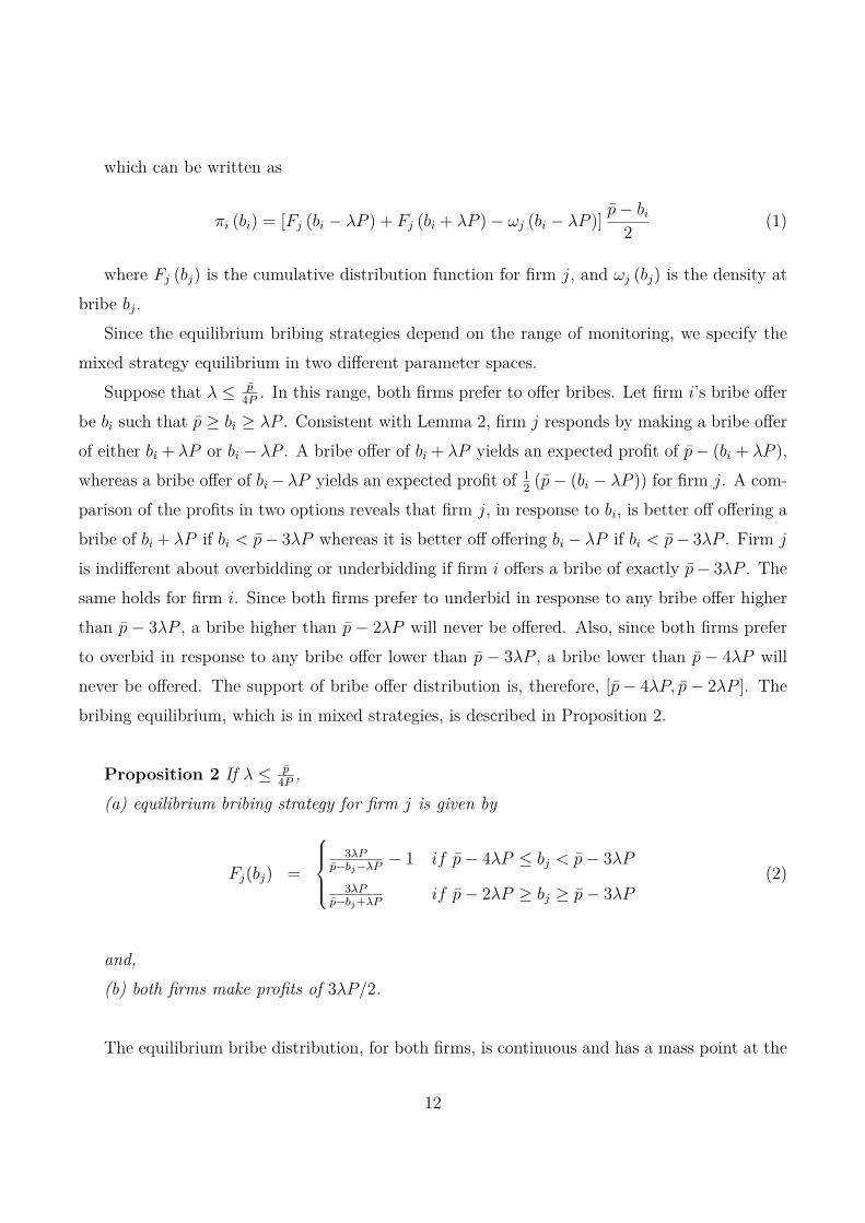
which can be written as

πi (bi) = [Fj (bi − λP ) + Fj (bi + λP )− ωj (bi − λP )] p̄− bi2 (1)

where Fj (bj) is the cumulative distribution function for firm j, and ωj (bj) is the density atbribe bj.

Since the equilibrium bribing strategies depend on the range of monitoring, we specify themixed strategy equilibrium in two different parameter spaces.

Suppose that λ ≤ p̄4P . In this range, both firms prefer to offer bribes. Let firm i’s bribe offer

be bi such that p̄ ≥ bi ≥ λP . Consistent with Lemma 2, firm j responds by making a bribe offerof either bi + λP or bi − λP . A bribe offer of bi + λP yields an expected profit of p̄− (bi + λP ),whereas a bribe offer of bi−λP yields an expected profit of 1

2 (p̄− (bi − λP )) for firm j. A com-parison of the profits in two options reveals that firm j, in response to bi, is better off offering abribe of bi + λP if bi < p̄− 3λP whereas it is better off offering bi − λP if bi < p̄− 3λP . Firm j

is indifferent about overbidding or underbidding if firm i offers a bribe of exactly p̄− 3λP . Thesame holds for firm i. Since both firms prefer to underbid in response to any bribe offer higherthan p̄ − 3λP , a bribe higher than p̄ − 2λP will never be offered. Also, since both firms preferto overbid in response to any bribe offer lower than p̄ − 3λP , a bribe lower than p̄ − 4λP willnever be offered. The support of bribe offer distribution is, therefore, [p̄− 4λP, p̄− 2λP ]. Thebribing equilibrium, which is in mixed strategies, is described in Proposition 2.

Proposition 2 If λ ≤ p̄4P ,

(a) equilibrium bribing strategy for firm j is given by

Fj(bj) =

3λP

p̄−bj−λP − 1 if p̄− 4λP ≤ bj < p̄− 3λP3λP

p̄−bj+λP if p̄− 2λP ≥ bj ≥ p̄− 3λP(2)

and,(b) both firms make profits of 3λP/2.

The equilibrium bribe distribution, for both firms, is continuous and has a mass point at the

12

indifference point. In equilibrium, both firms offer positive bribes with probability one. Theequilibrium is unique by construction. And it is straightforward to show, by contradiction, thatthe bribing strategies specified in Proposition 2 constitute Nash equilibrium.

It is of interest to look at how the equilibrium bribing strategies and profits respond to asmall change in monitoring. An increase in monitoring requires that firms overbid their rivalsby a larger amount if they wish to be selected with certainty. Given that both firms still offerbribes with probability one, it might appear counter-intuitive to see that profits are increasing inmonitoring λ. The intuition for this result is the following. Since firms must overbid by a largeramount to get selected with probability one they become less willing to do so. Firms becomeindifferent to overbidding or underbidding the rival firm at lower bribes. As a consequence,lower bribes are offered in equilibrium which results in higher profits for both firms. We canexpress each point in the support of the distribution in equation (2) in the form p̄− aλP , where2 ≥ a ≥ 4. This implies that the probability at each point in the support of bribe distributionis independent of λ.

We now look at the intermediate range of monitoring p̄4P ≤ λ ≤ p̄

2P . Given λ ≤ p̄2P , both

firms prefer to offer bribes if the other firm is not offering a bribe. Firms prefer to overbidby λP on any rival firm’s bid which is smaller than p̄

2 − λP . Since λ ≥ p̄4P , the alternative

strategy, as per Lemma 2, is to offer no bribes that yields lower profits. Here, firms also preferto underbid on any rival firm’s bid which is larger than λP . Since firms prefer to overbid onlyin response to bribe offers smaller than p̄

2 − λP , a bribe higher than p̄2 is not offered. If a firm

makes a bribe offer b ∈(p̄2 − λP, λP

)it must be in response to a bribe offer higher than p̄

2 . How-ever, since there are no bribe offers larger than p̄

2 there are no bribe offers made in the interval(p̄2 − λP, λP

). The support of the bribe offer distribution therefore is

[0, p̄2 − λP

]∪[λP, p̄2

]. The

equilibrium bribing strategies and profits, in this range of monitoring, are given in Proposition 3.

Proposition 3 If p̄4P ≤ λ ≤ p̄

2P ,(a) equilibrium bribing strategy for firm j is given by

Fj(bj) =

p̄+2λP2(p̄−bj−λP ) − 1 if 0 ≤ bj <

p̄2 − λP

p̄+2λP2p̄ if p̄

2 − λP ≥ bj ≥ λP

p̄+2λP2(p̄−bj+λP ) if λP ≥ bj ≥ p̄

2

13

and,(b) both firms make profits of p̄+2λP

4 .

The distribution is continuous in its support. There are two mass points for each firm, one atb = 0 and the other at b = p̄

2 − λP . This equilibrium is also unique; it can be easily shown thatthe bribing strategies specified in Proposition 3 constitute Nash equilibrium. Firms do not offerbribes with probability one in this range of monitoring. As monitoring is increased, firms offerbribes with smaller probability. This happens in response to the higher amount by which firmsmust overbid their bribe in order to be selected with certainty. The firm profits are increasingin monitoring but at a smaller rate compared to the rate of increase in the λ ≤ p̄

4P case. Thelower bound on bribes, at zero, causes profits to increase at a slower rate. We also note thatthere is no discontinuity in the bribe offer distribution or the firm profits at the boundaries ofthis parameter space.

2.2 Agent’s Selection Decision

Having described the price and bribe offer decisions in the entire range of monitoring, we nowlook at agent behavior. We are interested in an agent’s decision to select a non-deserving firmas it is this decision that hurts the buyer. The agent does not always select a non-deserving firmwhen she accepts a bribe. If the difference of bribes offered by the two firms is smaller thanthe expected loss that the agent incurs upon selecting a non-deserving firm, the agent simplyselects and accepts the bribe from the firm that is deserving. Since firms do not know if they aredeserving or not, they cannot condition their bribe payments on being non-deserving. The agentselects a firm with certainty only when the bribe offers are different by more than λP . However,selecting a firm with certainty does not imply that the agent is selecting a non-deserving firm.Note that the firms are deserving with probability 0.5. We can write the probability Pr withwhich the agent selects a non-deserving firm as

Pr = 12 prob(|bi − bj| > λP ) (3)

The probability Pr is computed using the equilibrium bribe distributions specified above.

14

We obtain the following results.

Proposition 4 The probability with which the agent selects a non-deserving firm(a) is strictly positive and independent of monitoring λ, if λ is sufficiently small (λ ≤ p̄

4P ),(b) first increases and then decreases to zero at λ = p̄

2P , when λ in increased beyond p̄4P , and

(c) is zero ∀ λ ≥ p̄2P .

These results are also presented graphically in Figure 2. We note two observations that werediscussed earlier. First, an increase in monitoring λ increases the cost of selecting a non-deservingfirm to the agent. And firms respond to higher monitoring by offering smaller or no bribes. Yetan increase in monitoring has no effect on an agent’s decision to select a non-deserving firmwhen monitoring is sufficiently small. Even more puzzling is the increase in Pr with monitoringin the intermediate range.

0 10

Pr

p̄4P

p̄2P

9ln(98 )−1

λ

Figure 2: Probability with which the agent selects non-deserving firm as a function of monitoring

The intuition for the above results is the following. If monitoring is sufficiently small (λ ≤ p̄4P )

both firms offer strictly positive bribes with probability one. When both firms offer bribes theagent often selects the deserving firm and accepts the bribe offered by it. Since both firms offerbribes for sure in this range of monitoring the probability with which the agent selects a non-

15

deserving firm does not change. If monitoring probability is increased beyond p̄4P , firms become

less likely to offer bribes. The agent is now faced with situations in which she receives a bribeoffer only from a non-deserving firm. This makes the selection of a non-deserving firm morelikely. As monitoring is further increased, firms become very unlikely to offer bribes. Therefore,the probability with which the agent selects a non-deserving firm also decreases. For a sufficientlylarge monitoring (λ ≥ p̄

2P ), firms do not offer bribes and, therefore, the agent does not select anon-deserving firm.

Insensitivity to or increase in dishonest behavior as a result of increased monitoring, orpenalty, has been widely reported in various contexts. Mazar, Amir, and Ariely (2008) find thedishonesty of test takers insensitive to monitoring. Several studies originating from Deci (1972)show in experiments that an increase in the monitoring can result in more dishonest behavior.Most related to our work is a study reported by Schulze and Frank (2003) where they showthat increase in monitoring can make an agent, making a procurement decision on behalf of aprincipal, more dishonest as a result of monitoring. Akerlof and Dickens (1982) and Bénabouand Tirole (2006) draw on the behavioral literature and present models to derive these results.We present a rational agent model without any behavioral assumptions and show that dishonestycan be insensitive to or can even be increasing in the monitoring. This result has importantimplications for buyers as well as firms in markets where corruption is prevalent.

2.3 Monitoring Decision

If a firm is fit the agent finds it deserving only with probability ρ. Therefore, if the agent makesan honest decision to select the deserving firm she selects a fit firm only with probability ρ. Thepayoff of the buyer is v with probability ρ and zero with probability 1−ρ. Similarly, if the agentselects a non-deserving firm the buyer gets a payoff of v with probability 1 − ρ and a payoff ofzero with probability ρ. The probability Pr with which the agent selects a non-deserving firmis discussed in the previous section. We can write the expected payoff of the buyer as

πG = Pr [(1− ρ) v] + (1− Pr) ρv − p̄− c (λ) (4)

We first look at πG |c(λ)=0. The expressions of Pr as given in the proof of Proposition 4 aresubstituted in equation (4) to get

16

πG |c(λ)=0 =

[3ρ− 1− 9 (2ρ− 1) ln

(98

)]v − p̄ if λ ≤ p̄

4P

(4ρ− 1) v2 + p̄[(2ρ−1)v−4λP ]

4λP − 2(2ρ−1)λPvp̄

if p̄4P ≤ λ ≤ p̄

2P

− (p̄+2λP )2(2ρ−1)v4λ2P 2 ln

((p̄−λP )(p̄+2λP )

p̄2

)ρv − p if λ ≥ p̄

4P

(5)

Note that λ enters πG |c(λ)=0 only through the probability Pr with which the agent selectsa non-deserving firm. It is now straightforward to understand how πG |c(λ)=0 changes withmonitoring λ. For λ ≤ p̄

4P , the probability Pr does not depend on λ, therefore πG |c(λ)=0 alsodoes not depend on λ. For p̄

4P ≤ λ ≤ p̄2P , the probability Pr first increases and then decreases

to zero, therefore πG |c(λ)=0 first decreases and then increases to maximum value at λ = p̄2P . For

λ ≥ p̄4P , it stays at its maximum value which is ρv − p̄. These results are graphically presented

in Figure 3. It is now simple to look at the buyer’s choice of λ under cost of monitoring c (λ).Buyer’s payoff at zero monitoring πG (λ = 0) is ρv− p̄− (2ρ− 1)

[9ln

(98

)− 1

]v. Since c (λ) > 0

for every λ > 0, any monitoring λ 6= 0 for which πG |c(λ)=0≤ πG (λ = 0) is not optimal. Also sincec′ (λ) > 0, optimal λ cannot be larger than p̄

2P . There is no extra benefit of increasing λ beyondp̄

2P to the buyer as the agent behaves as desired at all λ ≥ p̄2P . Therefore, buyer chooses optimal λ

from the set{

0,(λ̃, p̄

2P

]}, where λ̃ ∈

(p̄

4P ,p̄

2P

)is the monitoring at which πG |c(λ)=0= πG (λ = 0).

We see buyer as making one of the two choices. She either accepts corruption with zero anti-corruption enforcement or limits corruption, partially or fully, by setting a λ ∈

(λ̃, p̄

2P

]. The

buyer’s choice to limit the corruption or not depends on 4 which is defined as

4 ≡ (πG − πG (λ = 0)) |c(λ)=0 (6)

17

0 1

πG|c(λ)=0 ↑

p̄4P

p̄2P

ρv−p̄ →

λ̃ λ →

Figure 3: Buyer’s payoff with monitoring (for costless monitoring)

Further examination of the πG |c(λ)=0 function leads us to the following proposition:

Proposition 5 If c (λ) > 4 ∀λ ∈(λ̃, p̄

2P

], the buyer allows corruption with zero anti-

corruption enforcement (λ∗ = 0), else, she limits corruption by selecting a monitoring λ∗ ∈(λ̃, p̄

2P

].

The buyer sets the monitoring at either zero or at a sufficiently large value. A small mon-itoring does not make the buyer any better as the agent selects the non-deserving firm withthe same or higher probability. A buyer selecting a positive λ expects the agent to select thenon-deserving firm with a lower probability than she does when no monitoring is enforced. Thishappens only when λ > λ̃. The buyer setting a non-zero monitoring incurs a cost. If the cost ishigher than the benefit that the buyer enjoys due to more honest agent behavior, the buyer setsmonitoring at zero. If not, the buyer sets monitoring sufficiently large and limits corruption. Inthe case when the buyer allows corruption with zero anti-corruption enforcement the firms makezero profits. All the surplus is transferred to the agent in the form of bribes. However, if thebuyer limits corruption firms make expected profits of p̄+2λ∗P

4 . If the buyer eliminates corruptionby setting monitoring at p̄

2P the firms make expected profits of p̄2 , which is the highest profit that

18

the firms can make in this symmetric set-up.We next look at the role of c

(λ = p̄

2P

), which is relevant to the analysis presented in the next

section. Corruption is eradicated at the monitoring of λ = p̄2P . The buyer eradicates corruption

only if the cost at λ = p̄2P is smaller than the increase in profit the buyer enjoys as a result of

honest agent behavior compared to no monitoring. This gives

c(λ = p̄

2P

)< (2ρ− 1)

[9ln

(98

)− 1

]v (7)

The above equation, while necessary, is not sufficient for corruption eradication. There may be aλ ∈

(λ̃, p̄

2P

)that dominates eradication. While the condition c

(λ = p̄

2P

)> (2ρ− 1)

[9ln

(98

)− 1

]v

implies that corruption is not eradicated, equation (7) implies that the buyer limits the corrup-tion, partially or completely.

Buyers either choose to be ignorant or commit to take drastic measures to limit corruption.It is never optimal for the buyer to set monitoring in the interval

(0, λ̃

). A small anti-corruption

effort does not reduce corruption.13 Singapore and Hong Kong were once corruption infested.However, as they implemented drastic measures to combat corruption, they have almost com-pletely eradicated it. The efforts to limit corruption in many other emerging economies appearhalf-hearted. The impact on prevalence of corruption is therefore little, if any.

3 Unilateral Control

In this section, we consider that one of the firms, say firm i, as required by the law in its homecountry, does not offer bribes to the agent. The structure and timing of the game is exactly asin the previous section. As before both firms make a price bid of p̄. The firm j either does notoffer a bribe or it offers a bribe of λP . We assume that if firm j is indifferent between offeringand not offering a bribe it does not offer a bribe. If firm j does not offer any bribe the agentselects the firm that is deserving. Both firms make an expected profit of p̄2 in this case. However,if firm j offers a bribe of λP the agent selects firm j with probability one. Any lower bribe doesnot make the agent select a non-deserving firm j. Any higher bribe is strictly dominated by λP .If firm j offers a bribe it makes a profit of p̄− λP and firm i makes zero profit.

13Uslaner (2008) talks about some studies indicating evidence of stickiness of corruption and its effects.

19

If λ ≥ p̄2P , in equilibrium both firms offer no bribes. A possible deviation for the firm j is to

offer a bribe of λP and make a profit of p̄ − λP . However, given λ ≥ p̄2P the deviation is not

more profitable than the equilibrium strategy. Similarly, if λ < p̄2P , firm j offers a bribe of λP in

equilibrium. The buyer gets her valuation v with probability ρ if the agent selects the deservingfirm, whereas she gets v only with probability 1

2 if the agent selects firm j with certainty. Thepayoff of the buyer is

πuG =

ρv − p̄− c (λ) if λ ≥ p̄

2P

12v − p̄− c (λ) if λ < p̄

2P

These payoffs, assuming c (λ) = 0, are shown in Figure 4. We can now look at the buyer’sdecision to set monitoring.

0 10

πG|c(λ)=0 ↑

p̄4P

p̄2P

12v−p̄ →

ρv−p̄ →

λ̃ λ →

12 (2ρ− 1)v

l (2ρ− 1)(9ln(98 )− 1)v

Without unilateral controlWith unilateral control

Figure 4: Buyer’s payoff with monitoring with and without unilateral anti-corruption control(for costless monitoring)

The buyer either eliminates corruption by setting monitoring at p̄2P or sets monitoring at

zero. Since c′ (λ) > 0, the buyer does not set any other monitoring. The buyer’s decision to setmonitoring depends only on the cost of monitoring at λ = p̄

2P . If c(λ = p̄

2P

)<(ρ− 1

2

)v, the

20

buyer sets monitoring at p̄2P and eliminates corruption. However, if c

(λ = p̄

2P

)>(ρ− 1

2

)v, the

buyer sets monitoring at zero. We ignore the equality case in which the buyer can mix betweenthe two monitorings. A comparison of firm i’s profits with and without unilateral control leadsus to the following proposition:

Proposition 6 A unilateral control on bribing on a firm in a corrupt but competitive marketmay increase its profits if c

(λ = p̄

2P

)≤(9ln

(98

)− 1

)(2ρ− 1) v, would definitely increase its

profits if(9ln

(98

)− 1

)(2ρ− 1) v < c

(λ = p̄

2P

)< 1

2 (2ρ− 1) v, and may decrease its profits ifc(λ = p̄

2P

)≥ 1

2 (2ρ− 1) v.

One striking result in the above proposition is that a unilateral anti-corruption control canactually benefit the firm that is being restricted from offering a bribe. A unilateral control onone firm eliminates competition in bribes. The firm that is not controlled can offer just λP andbe selected with certainty. This makes the selection of a non-deserving firm by the agent morelikely. The buyer may, strategically, set a higher monitoring to discourage bribery by the firmthat is not controlled. This results in higher profits for a unilaterally controlled firm. A firmunder unilateral control can be worse off as well. This happens if, in the absence of unilateralcontrol, the buyer sets a non-zero monitoring, but with unilateral control the buyer sets zeromonitoring. A steep increase in the cost before p̄

2P can make the elimination of corruptionunattractive for the buyer. If buyer’s decision to set monitoring does not change as unilateralcontrol is introduced, the profits of the controlled firm remain unchanged.

The firm that is not controlled benefits from the unilateral control on the other firm. Forthe controlled firm the benefit comes as a result of the buyer setting higher monitoring. Thefirm that is not controlled also benefits when the buyer sets zero monitoring. Without unilateralcontrol all the surplus was transferred to the agent in the process of competitive bribing. Butwith unilateral control on the other firm, a firm makes higher profits as it offers a bribe of onlyλP . We think that claims about competitive disadvantage faced by the controlled firm originatefrom this comparison where the buyer sets monitoring at zero. If the buyer sets monitoring atzero the firm that is not controlled is selected by the agent and makes higher profits than thecontrolled firm, which makes zero profits. However, what is not taken into consideration is thateven if the unilateral control is not there the firm would still make zero profits.

21

The higher profits for the controlled firm results due to the buyer’s choice of higher moni-toring. There is some evidence of such increased monitoring. Gillespie (1987) finds evidence ofthis in the Middle East after 1977. It comes to us as no surprise that most empirical studiesfind no evidence of competitive disadvantage posed by the FCPA of 1977. We also note that theenforcement of the FCPA has increased drastically in recent years.14 It is interesting to observerecent anti-corruption efforts in BRIC15 countries. Brazil enacted the Freedom of InformationLaw of 2011, which is a step forward in the direction of reducing corruption. Russia signed theOECD’s Anti-Bribery Convention in 2012. An anti-corruption movement started in India inyear 2010 that seeks strong legislation and enforcement against corruption. China implementeda stricter anti-bribery law in 2011. We have no reason to believe that these efforts are only inresponse to the increased FCPA enforcements. However, we believe that this increase in theFCPA enforcements will make the U.S. firms better off as foreign governments take measures tolimit corruption.

4 Conclusion

This paper studies competition in a corrupt market. The buyer lacks the expertise or theinformation needed to evaluate firms. An agent selects the firm for the buyer. This createsscope of corruption. Sometimes, the agent selects a non-deserving firm in exchange for bribes.Both the buyer and the agent are strategic. The competitive bidding behavior of the ex-antesymmetric firms is examined. A pure strategy Nash equilibrium in bribes exists only if themonitoring of the agent is sufficiently large. The expected penalty to the agent is so large thatfirms find it unprofitable to offer such a large bribe. The agent selects the deserving firm.

If monitoring is not sufficiently large the bribe offer equilibrium is in mixed strategies. Theagent selects a non-deserving firm if its bribe offer is sufficiently larger than the bribe offer of thedeserving firm. Otherwise, the agent accepts the bribe offer of the deserving firm and selects it.We find that an increase in the monitoring does not always result in more honest agent behavior.It sometimes backfires. This agent behavior originates due to the endogenous bribe offers madeby firms.

14According to a report published by Shearman & Sterling LLP (2012), the corporate FPCA cases increasedfrom 14 between 2002 and 2006 to 70 between 2007 and 2011.

15Brazil, Russia, India and China, the major emerging economies, are collectively referred to as BRIC.

22

The non-monotonic agent behavior in response to changes in the monitoring, or anti-corruptionefforts, makes it difficult for the buyer to reduce corruption. If bribery is prevalent, a smallchange in the monitoring does not reduce corruption. The buyer must take drastic measures ifshe wishes to curb corruption.

We find that a unilateral anti-corruption control on a firm, such as the FCPA of 1977, canresult in higher profits for the controlled firm. A direct effect of the anti-corruption control isthat it makes the foreign government worse off by making the selection of a non-deserving firmby the agent more likely. The foreign government may strategically set a higher monitoring.Profits of the controlled firm may increase as a result. We resolve the disconnect between theprevailing perception about the FCPA in the business community and findings of the empiricalstudies. Higher monitoring set by the foreign government in response to the FCPA is the keyto higher profits of a controlled firm. There is some evidence of increase in anti-corruptionenforcements by foreign governments in response to the FCPA.

The findings of this work have important implications for firms conducting business in emerg-ing markets, buyers in these markets and the US government. US firms should note that thedebate about the competitive disadvantage posed by the FCPA may be misplaced. Also, whilegovernments in the emerging economies may be disinterested in reducing corruption, it is in theinterest of firms to support the anti-corruption efforts. Buyers should either ignore corruptionor take drastic measures to limit it. Implication for the US government is that the unilateralanti-corruption control should be aggressively enforced as it not only reduces corruption butmay also increase profits of US firms. The model can be applied to various settings where anagent makes a decision, such as awarding certification, issuing permit, law enforcement or pro-curement, on behalf of a principal and the principal lacks the expertise or the information tomake the same decision.

23

Appendix

Proof of Proposition 1

Profit of each firm in equilibrium is p̄2 . The best possible deviation for a firm is to make a bribe

offer of λP and get selected with probability one. Profit of the firm under this deviation isp̄ − λP . However, deviation is not profitable given λ ≥ p̄

2P . The agent also has no profitabledeviations. Hence, no bribes are offered in equilibrium.

Now, we show that there is no pure strategy Nash equilibrium for λ < p̄2P .

Suppose(b∗i , b

∗j

)is a pair of Nash equilibrium strategies. Then there is no other bi (i = 1, 2)

such that πi(bi, b

∗j

)> π∗i

(b∗i , b

∗j

). We show that such a bi exists.

If b∗i = b∗j , any of the firms can strictly benefit by cutting the bribe offer by small ε.If b∗i > b∗j (the proof for b∗i < b∗j is analogous),Case (1) b∗i > b∗j + λP

Since firm i gets selected with probability one, πi(b∗i , b

∗j

)= p̄− b∗i .

∃ ε such than bi = b∗i − ε and bi > bj + λP . Firm i can make larger profits by offering bi.Case (2) b∗i ≤ b∗j + λP

Agent picks firm i only when it is deserving (i.e. with probability 0.5). Equilibrium profitsin this case are π∗i

(b∗i , b

∗j

)= 1

2 (p̄− b∗i ).∃ ε such that bi = b∗i − ε and firm i is selected by agent whenever it is deserving. This

generates strictly higher profits for the firm i.Therefore, there is no Nash equilibrium in pure strategies.

Proof of Proposition 2

We prove Proposition 2 in following steps.Step 1 If firm i offers p̄ − 3λP firm j would be indifferent between overbidding and under-

bidding.Suppose firm i bids b̂i. Firm j can bid b̂i+λP (+ infinitesimally small ε) and get selected with

probability one or bid b̂i − λP and get selected with probability 12 . Firm j would be indifferent

24

if

12[p̄−

(b̂i − λP

)]= p̄−

(b̂i + λP

)b̂i = p̄− 3λP

If bi > p̄− 3λP firm j offers bj = bi− λP , whereas if bi < p̄− 3λP firm j offers bj = bi + λP .Step 2 f (bi) = 0 for bi > p̄− 2λP and for bi < p̄− 4λP .Suppose bi > p̄−2λP . This can happen only if firm i offers bj+λP in response to bj > p̄−3λP .

However, for any bj > p̄ − 3λP , as established in Step 1, firm i responds by offering bj − λP .Now suppose bi < p̄ − 4λP . This implies that firm i must be offering a bribe of bj − λP inresponse to bj < p− 3̄λP . But, following Step 1, firm i should be offering bj + λP . Both caseslead to contradiction.

Step 3 The equilibrium bribing strategy sets S∗i and S∗j are convex.We prove this by contradiction. Suppose there is an interval I =

(bk, bh

), where p̄− 4λP <

bk < bh < p̄− 2λP and firm i offers bi ∈ I with probability zero.Claim 1 Firm j offers bj ∈ (I + λP ) ∪ (I − λP ) with probability zero.(a) If bh ≤ p̄− 3λP , f (bj) = 0 for bj ∈ I − λP (from Step 2)Suppose firm j offers b′ ∈ I + λP with positive probability. Since f (bi) = 0 for bi ∈ I,

firm j can offer inf (I + λP ) and make higher profit than offering any b′ ∈ I + λP . Therefore,f (bj) = 0 for bj ∈ (I + λP ) ∪ (I − λP ).

(b) Now if bk > p̄− 3λP , f (bj) = 0 for bj ∈ I + λP (from Step 2)Suppose firm j offers b′ ∈ I − λP with positive probability. Since f (bi) = 0 for bi ∈ I,

firm j can offer inf (I − λP ) and make higher profit than offering any b′ ∈ I − λP . Therefore,f (bj) = 0 for bj ∈ (I + λP ) ∪ (I − λP ).

(c) Lastly, if bh > p̄ − 3λP > bk, firm j will be better off offering inf (I + λP ) insteadof any bj ∈ (I + λP ). If bj ∈ (I − λP ), since f (bi) = 0 for bj < p̄ − 4λP , it must be thatbj ∈ [p̄− 4λP, bh− λP ). Note that, ∀ bi < bk firm j prefers to make a bribe offer bj = bi + λP >

p̄− 3λP , and ∀ bi > bh firm j prefers to make a bribe offer bj = bi − λP > bh − λP . Therefore,given bi /∈ I and firm j offers bj ∈

[bh − λP, bk + λP

].

Therefore, f (bj) = 0 for bj ∈ (I + λP ) ∪ (I − λP ).Claim 2 Firm i offering bi ∈ I with probability zero and firm j offering bj ∈ (I + λP ) ∪

25

(I − λP ) with probability zero constitutes a contradiction.Let us represent b̃ ≡ inf

(b > bh

).

Using equation (1), we can write

πi(b̃)

=[Fj(b̃+ λP

)+ Fj

(b̃− λP

)− ωj

(b̃− λP

)] p̄− b̃2

πi(bk)

=[Fj(bk + λP

)+ Fj

(bk − λP

)− ωj

(bk − λP

)] p̄− bk2

But since Fj(b̃+ λP

)= Fj

(bk + λP

), Fj

(b̃− λP

)= Fj

(bk − λP

)and ωj

(bk − λP

)= 0,

profit of firm i when offering bk is strictly higher than offering b̃ contradicting the assumption ofan equilibrium.

Step 4 There can be a mass point in the bribe distribution of a firm only at b = p̄− 3λP .Suppose firm j has a mass point at b∗ ∈ [p̄− 4λP, p̄− 3λP ) equal to ω.We can write

πi (b∗ + λP + ε) = [Fj (b∗ + 2λP + ε) + Fj (b∗ + ε)− ωj (b∗ + ε)] p̄− (b∗ + λP + ε)2

πi (b∗ + λP − ε) = [Fj (b∗ + 2λP − ε) + Fj (b∗ − ε)− ωj (b∗ − ε)] p̄− (b∗ + λP − ε)2

Subtracting 2nd equation from 1st we get

πi (b∗ + λP + ε)− πi (b∗ + λP − ε) = p̄− (b∗ + λP )2 [Fj (b∗ + 2λP + ε)− Fj (b∗ + 2λP − ε)

+Fj (b∗ + ε)− Fj (b∗ − ε)− ωj (b∗ + ε) + ωj (b∗ − ε)]

−ε2 [Fj (b∗ + 2λP + ε) + Fj (b∗ + ε)− ωj (b∗ + ε)

+Fj (b∗ + 2λP − ε) + Fj (b∗ − ε)− ωj (b∗ − ε)]

For small enough ε > 0,

πi (b∗ + λP + ε)− πi (b∗ + λP − ε) > 0

and firm i by shifting some density from bottom to top of b∗ + λP can be strictly better off. Sothere can not be a mass point at b∗ ∈ [p̄− 4λP, p̄− 3λP ).

26

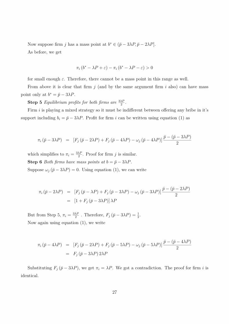
Now suppose firm j has a mass point at b∗ ∈ (p̄− 3λP, p̄− 2λP ].As before, we get

πi (b∗ − λP + ε)− πi (b∗ − λP − ε) > 0

for small enough ε. Therefore, there cannot be a mass point in this range as well.From above it is clear that firm j (and by the same argument firm i also) can have mass

point only at b∗ = p̄− 3λP .Step 5 Equilibrium profits for both firms are 3λP

2 .Firm i is playing a mixed strategy so it must be indifferent between offering any bribe in it’s

support including bi = p̄− 3λP . Profit for firm i can be written using equation (1) as

πi (p̄− 3λP ) = [Fj (p̄− 2λP ) + Fj (p̄− 4λP )− ωj (p̄− 4λP )] p̄− (p̄− 3λP )2

which simplifies to πi = 3λP2 . Proof for firm j is similar.

Step 6 Both firms have mass points at b = p̄− 3λP .Suppose ωj (p̄− 3λP ) = 0. Using equation (1), we can write

πi (p̄− 2λP ) = [Fj (p̄− λP ) + Fj (p̄− 3λP )− ωj (p̄− 3λP )] p̄− (p̄− 2λP )2

= [1 + Fj (p̄− 3λP )]λP

But from Step 5, πi = 3λP2 . Therefore, Fj (p̄− 3λP ) = 1

2 .Now again using equation (1), we write

πi (p̄− 4λP ) = [Fj (p̄− 2λP ) + Fj (p̄− 5λP )− ωj (p̄− 5λP )] p̄− (p̄− 4λP )2

= Fj (p̄− 3λP ) 2λP

Substituting Fj (p̄− 3λP ), we get πi = λP . We got a contradiction. The proof for firm i isidentical.

27

Step 7 Both firms have point mass of 14 at b = p̄− 3λP .

Using equation (1), we can write

πi (p̄− 2λP ) = [1 + Fj (p̄− 3λP )− ωj (p̄− 3λP )] p̄− (p̄− 2λP )2

= [1 + Fj (p̄− 3λP )− ωj (p̄− 3λP )]λP

similarly,

πi (p̄− 4λP ) = Fj (p̄− 3λP ) 2λP

Using the result from Step 5, we solve two equations to get Fj (p̄− 3λP ) = 34 , and ωj (p̄− 3λP ) =

14 . The proof for firm i is identical.

Step 8 Equilibrium bribing strategy for firm j is given by

Fj(bj) =

3λP

p̄−bj−λP − 1 if p̄− 4λP ≤ bj < p̄− 3λP3λP

p̄−bj+λP if p̄− 2λP ≥ bj ≥ p̄− 3λP

Using equation (1) and Step 5, we can write

[Fj (bi − λP ) + Fj (bi + λP )− ωj (bi − λP )] p̄− bi3λP = 1

Using above equation and the results from Step 2 and Step 7, we can write

Fj (bi + λP ) = 3λPp̄−bi

if bi ≤ p̄− 3λP

Fj (bi − λP ) = 3λPp̄−bi− 1 if p̄− 2λP > bi ≥ p̄− 3λP

Fj (bi − λP ) = 34 if bi = p̄− 2λP

Applying appropriate transformations to above three equations proves Step 8.

28

Proof of Proposition 3

Since the proof of Proposition 3 is similar to that of proposition 2, we only provide the stepshere.

Step 1 If a firm makes a bribe offer of p̄2 − λP the other firm will be indifferent between

offering a bribe higher by λP and offering no bribe. It prefers to overbid on smaller offers. Thisholds given λ ≥ p̄

4P .Step 2 If a firm makes a bribe offer b ≥ λP the other firm prefers to offer b− λP . This also

holds given λ ≥ p̄4P .

Step 3 f (b) = 0 for b > p̄2 and for b ∈

(p̄2 − λP, λP

).

Step 4 There are no holes in the interval[0, p̄2 − λP

]and in the interval

[λP, p̄2

].

Step 5 There is no density at b = λP for both firms. Because, if there is firms can strictlybenefit by moving density from b = λP to b = p̄

2 − λP .Step 6 Both firms make profits of p̄+2λP

4 . This is obtained by evaluating equation (1) atb = p̄

2 − λP .Step 7 There is a mass point of 4λP−p̄

2(p̄−λP ) at b = 0 and a mass point of p̄−2λP2p̄ at b = p̄

2 − λPfor both firms.

Step 8 Using equation (1) and Step 6 we can write

[Fj (bi − λP ) + Fj (bi + λP )− ωj (bi − λP )] 2 (p̄− bi)p̄+ 2λP = 1

Using Step 2, Step 7, above equation and applying appropriate transformations we get thecdf given in Proposition 3.

Proof of Proposition 4

(a) λ ≤ p̄4P case

Using equation (3), we can write Pr as

Pr = 12

ˆ p̄−3λP

p̄−4λP[1− Fj (bi + λP )] fi (bi) dbi + 1

2

ˆ p̄−2λP

p̄−3λP[Fj (bi − λP )] fi (bi) dbi

= 12

ˆ p̄−3λP

p̄−4λP

(1− 3λP

p̄− bi

)3λP

(p̄− bi − λP )2dbi + 12

ˆ p̄−2λP

p̄−3λP

(3λPp̄− bi

− 1)

3λP(p̄− bi + λP )2dbi

29

where fi(bi) is the pdf of the bribe offer and is obtained by differentiating the cdf describedin Proposition 2. Simplifying the above equation we get Pr = 9 ln

(98

)− 1.

(b) p̄4P ≤ λ ≤ p̄

2P caseUsing equation (3), we can write Pr as

Pr = 12

ωi (0) [1− Fj (λP )] +ˆ p̄

2−λP

0[1− Fj (bi + λP )] fi (bi) dbi

+ˆ p̄

2

λP

[Fj (bi − λP )] fi (bi) dbi

= 1

2

4λP − p̄2 (p̄− λP )

(1− p̄+ 2λP

2p̄

)+ˆ p̄

2−λP

0

(1− p̄+ 2λP

2 (p̄− bi)

)p̄+ 2λP

2 (p̄− bi − λP )2dbi

+ˆ p̄

2

λP

(p̄+ 2λP2 (p̄− bi)

− 1)

p̄+ 2λP2 (p̄− bi + λP )2dbi

where pdf is obtained by differentiating the cdf described in Proposition 3. Simplifying the

above expression gives

Pr = −(p̄− 2λP ) (p̄+ 4λP )2p̄λP + (p̄+ 2λP )2

2λ2P 2 ln

((p̄+ 2λP ) (p̄− λP )

p̄2

)(8)

It is straightforward to check that

Pr(λ = p̄

4P

)= 9 ln

(98

)− 1 ; Pr

(λ = p̄

2P

)= 0

and,

∂Pr

∂λ|λ= p̄

4P> 0 ; ∂Pr

∂λ|λ= p̄

2P< 0

The maxima of the Pr function is numerically calculated. It is found to be at λ ' p̄3P .

(c) λ ≥ p̄2P case

Firms do not offer bribes if monitoring is sufficiently large (λ ≥ p̄2P ). The agent, therefore,

30

does not select a non-deserving firm. The probability Pr is zero in this range.

Proof of Proposition 5

From equation (5), 4 is zero for λ ≤ p̄4P . If p̄

4P ≤ λ ≤ p̄2P , substituting the expressions of

πG |c(λ)=0 and πG (λ = 0) |c(λ)=0 from equation (5) to equation (6) we get

4 =[ [p̄2−8λ2P 2+2p̄λP(18ln( 9

8)−1)]4p̄λP − (p̄+2λP )2

4λ2P 2 ln(

(p−λP )(p̄+2λP )p̄2

)](2ρ− 1) v

The difference 4 is negative for all λ ∈(p̄

4P , λ̃). It is zero at λ = λ̃ and increases to(

9ln(

98

)− 1

)(2ρ− 1) v at λ = p̄

2P .In the range λ ≥ p̄

2P , it can be shown using equation (5) that4 stays at(9ln

(98

)− 1

)(2ρ− 1) v.

The buyer would, therefore, set a λ only from the set{

0,(λ̃, p̄

2P

]}. Since 4 the extra benefit

of setting a non-zero λ, a cost of monitoring higher than 4 would discourage the buyer fromsetting that λ. If it is the case for all λ ∈

(λ̃, p̄

2P

]the buyer sets the monitoring at zero. If

c (λ) < 4 for some λ 6= 0, the buyer sets a non-zero λ which maximizes her payoff.

Proof of Proposition 6

Note that the difference in buyer’s payoff, when setting λ = p̄2P and when setting λ = 0, is given

by(9ln

(98

)− 1

)(2ρ− 1) v if there no unilateral control on firm i. It is given by 1

2 (2ρ− 1) v ifthe firm i is unilaterally controlled. We now look at the three cases.

(a) c(λ = p̄

2P

)≤(9ln

(98

)− 1

)(2ρ− 1) v case

The profits of firm i under unilateral control is p̄2 . In the absence of the unilateral control

firm i’s profit is p̄+2λ∗P4 , where λ∗ ∈

(λ̃, p̄

2P

]. The maximum profit of firm i in absence of uni-

lateral control could be p̄2 if λ∗ = p̄

2P . Therefore, in this range of cost curves the profit for firmi as a result of unilateral control on bribes will either not change or increase. It can not decrease.

(b)(9ln

(98

)− 1

)(2ρ− 1) v < c

(λ = p̄

2P

)< 1

2 (2ρ− 1) v caseThe firm i still makes p̄

2 under unilateral control since buyer eliminates corruption. However,if there is no unilateral control in this range of cost curves the buyer does not find it optimal to

31

completely eliminate corruption resulting in profits of strictly lower than p̄2 . Here, the controlled

firm strictly benefits as a result of unilateral control.

(c) c(λ = p̄

2P

)≥ 1

2 (2ρ− 1) v caseThe firm i makes zero profits under unilateral control. In the absence of the unilateral

control the buyer does not find it optimal to completely eliminate corruption. However, for costcurve that become very steep as they approach λ = p̄

2P the buyer might find it optimal to set aλ ∈

(λ̃, p̄

2P

). Therefore, in this case the controlled firm will either make the same or lower but

not higher profits compared to if it was not controlled.

32

References

Akerlof, G. A., and W. T. Dickens (1982): “The Economic Consequences of CognitiveDissonance,” The American Economic Review, 72(3), pp. 307–319.

Beck, P. J., M. W. Maher, and A. E. Tschoegl (1991): “The Impact of the ForeignCorrupt Practices Act on US Exports,” Managerial and Decision Economics, 12(4), pp. 295–303.

Bénabou, R., and J. Tirole (2006): “Incentives and Prosocial Behavior,” American Eco-nomic Review, 96(5), 1652–1678.

Branco, F., and J. M. Villas-Boas (2012): “Competitive Vices,” working paper.

Burguet, R., and Y.-K. Che (2004): “Competitive Procurement with Corruption,” TheRAND Journal of Economics, 35(1), pp. 50–68.

Compte, O., A. Lambert-Mogiliansky, and T. Verdier (2005): “Corruption and Com-petition in Procurement Auctions,” The RAND Journal of Economics, 36(1), pp. 1–15.

Deci, E. L. (1972): “Intrinsic Motivation, Extrinsic Reinforcement, and Inequity,” Journal ofPersonality and Social Psychology, 22(1), 113–120.

Durbin, E., and G. Iyer (2009): “Corruptible Advice,” American Economic Journal: Mi-croeconomics, 1(2), 220–242.

Gillespie, K. (1987): “The Middle East Response to the U.S. Foreign Corrupt Practices Act,”California Management Review, 29, 4.

Graham, J. L. (1984): “The Foreign Corrupt Practices Act: A New Perspective,” Journal ofInternational Business Studies, 15(3), pp. 107–121.

Hauser, J. R., D. I. Simester, and B. Wernerfelt (1997): “Side Payments in Marketing,”Marketing Science, 16(3), pp. 246–255.

Inderst, R., and M. Ottaviani (2012): “Competition through Commissions and Kickbacks,”American Economic Review, 102(2), 780–809.

33

Jain, A. K. (2001): “Corruption: A Review,” Journal of Economic Surveys, 15(1), 71–121.

James R. Hines, J. (1995): “Forbidden Payment: Foreign Bribery and American BusinessAfter 1977,” NBER Working Paper No. 5266.

Kaikati, J. G., and W. A. Label (1980): “American Bribery Legislation: An Obstacle toInternational Marketing,” Journal of Marketing, 44(4), pp. 38–43.

Mazar, N., O. Amir, and D. Ariely (2008): “The Dishonesty of Honest People: A Theoryof Self-Concept Maintenance,” Journal of Marketing Research, 45(6), 633–644.

Mookherjee, D., and I. P. L. Png (1995): “Corruptible Law Enforcers: How Should TheyBe Compensated?,” The Economic Journal, 105(428), pp. 145–159.

Narasimhan, C. (1988): “Competitive Promotional Strategies,” The Journal of Business,61(4), pp. 427–449.

Rose-Ackerman, S. (1975): “The economics of corruption,” Journal of Public Economics, 4,187–203.

Scharfstein, D. S., and J. C. Stein (1990): “Herd Behavior and Investment,” The AmericanEconomic Review, 80(3), pp. 465–479.

Schulze, G. G., and B. Frank (2003): “Deterrence versus intrinsic motivation: Experimen-tal evidence on the determinants of corruptibility,” Economics of Governance, 4, 143–160,10.1007/s101010200059.

Shleifer, A., and R. W. Vishny (1993): “Corruption,” The Quarterly Journal of Economics,108, 599–617.

Uslaner, E. M. (2008): Corruption, Inequality, and the Rule of Law. Cambridge UniversityPress.

Varian, H. R. (1980): “A Model of Sales,” The American Economic Review, 70(4), pp. 651–659.

Wei, S.-J. (2000): “How Taxing is Corruption on International Investors?,” Review of Eco-nomics and Statistics, 82, 1–11.

34