competition in cloud computing
TRANSCRIPT

Competition in Cloud Computing
Juan Camilo Castillo Assistant Professor of Economics
University of Pennsylvania
Amit Gandhi
Professor of Economics University of Pennsylvania
Economics of Digital Services (EODS) is an initiative of the University of Pennsylvania’s Center for
Technology, Innovation and Competition (CTIC) and The Warren Center for Network & Data Sciences. Its
aim is to generate independent research on the economics of digital services and the role of data and
algorithms in the business strategies of digital platforms. The initiative was funded by a major grant from the
John S. and James L. Knight Foundation to support scholarly inquiry and novel approaches in the evolving
digital age.
To learn more about the initiative, visit www.law.upenn.edu/digitaleconomics/.
Center for Technology, Innovation and Competition (CTIC)
CTIC is an interdisciplinary academic center at the University of Pennsylvania Carey Law School that
bridges law and technology for academia and students. Focusing on intellectual property, antitrust, internet
law, and privacy law and policy. CTIC delivers foundational research that shapes the way legislators,
regulatory authorities, and scholars develop policy and regulatory frameworks. CTIC also produces
programming that explores the full range of scholarly perspectives, engages with industry experts, and
prepares the next generation of technology scholars, lawyers, and policymakers.
www.pennCTIC.org
The Warren Center for Network & Data Sciences
The University of Pennsylvania’s Warren Center fosters research and innovation in interconnected social,
economic, and technological systems. Collaborating with Penn affiliates, it focuses on the role of data and
algorithms to understand networked systems and how they can improve lives. The center also produces
events that connect researchers, students, and entrepreneurs across the spectrum of network science.
www.warrencneter.upenn.edu
Competition in Cloud Computing∗
Juan Camilo Castillo† Amit Gandhi‡
September 1, 2021
Abstract
In this paper we investigate whether cloud computing markets are com-
petitive. We assemble a dataset of the historic prices of Infrastructure as a
Service products from the three largest cloud computing providers. We find
that prices are surprisingly sticky, with most products experiencing zero price
changes over a six year period. Newer generations of products are introduced
at lower price levels, but prices go down much more slowly than semiconduc-
tor prices. These patterns differ from what one would expect in a competitive
environment. We set up a model of the cloud computing market that we will
estimate in future versions in order to quantify the welfare losses from lack of
competition.
Preliminary and incomplete. Please do not cite or distributewithout permission of the authors.
1 Introduction
Cloud computing is a paradigm shift in the way companies use information technol-
ogy (IT) to satisfy their computing and data storage needs. Traditionally, they had
∗We are grateful to Aarón Mora and Caleb Shack for excellent research assitance. This researchwas supported by the University of Pennsylvania Center for Technology, Innovation, and Competi-tion and by The Warren Center for Network and Data Sciences.†Economics Department, University of Pennsylvania. E-mail: [email protected]‡Economics Department and The Wharton School, University of Pennsylvania. E-mail: ak-
1

to install their own computing infrastructure and pay upfront for expensive soft-
ware licenses, which required costly capital expenditures with high lead times. A
new possibility emerged around 2005 with cloud computing providers like Amazon
Web Services (AWS), Microsoft Azure, and Google Cloud Platform (GCP), which
sell data storage, computing power, and software on-demand. Cloud providers
transform IT into a variable cost, giving companies a large degree of flexibility and
allowing them to scale up quickly and experiment with new technologies at a low
cost. Businesses ranging from technology startups to well-established blue chip
companies have thus been avid adopters of cloud computing, which is already a
$270 billion market—accounting for over 10% of global IT spending—and has been
growing over 20% per year (Gartner, 2021).
One open question that has important social consequences is whether cloud
computing markets are competitive. The basic infrastructure products offered by
cloud providers—computing power and data storage—are essentially commodities,
suggesting a highly competitive environment with low switching costs. However,
there are reasons to think the market is not that competitive. It is highly concen-
trated: one dominant player (AWS) has around 48% market share, and a few sec-
ondary players have 16%, 8%, and 4% market shares (Azure, Alibaba Cloud, and
GCP, respectively; Su, 2021). Concentration might be a result of providers’ strategy
of offering bundles of services that include infrastructure products as well as more
differentiated services like software and customer support that is tailored to specific
clients, which often leads to customer lock-in.
The goal of this project is to quantify the degree of competitiveness in the cloud
computing market and to measure the welfare losses due to any lack of competi-
tiveness. We collect a dataset of historic prices over the last six years of computing
infrastructure products from the three main players (AWS, Azure, and GCP), and
complement it with a dataset of usage by Azure customers. We present a descriptive
analysis that documents the main patterns in these companies’ pricing schemes. In
future versions of this project, we will also present a structural analysis of the cloud
computing market that will allow us to measure the degree of competition and to
quantify welfare.
We first document all dimensions over which prices vary for cloud services. We
2

focus on the prices charged by AWS for virtual machines (VMs), fully-functioning
computers that are hosted in the cloud.1 We find that prices are linear in the size of
the machine: doubling the number of cores and the amount of RAM memory leads
to a price that is higher by a factor of two. Other than the size of the machine, the
drivers of price variation from most important to least important are pre-installed
software (such as SQL), the type of VM (the type of processor, the memory per core,
whether it has GPUs, etc.), the operating system, and the physical location of the
virtual machine.
We then focus on price variation over time. Our first main finding is that price
changes are extremely rare. 90% of the products we observe experience no price
changes over the whole period of our data. Those products that do have price
changes exhibit only a couple of price reductions, none of which is larger than 10%.
This is striking given that this is a market that rents out semiconductors, a product
whose prices fall drastically over time (Byrne et al., 2018b).
We also analyze the price levels at which new products are introduced. Over
time, cloud providers introduce newer VMs with more advanced processors. We
find that each newer generation is introduced at a lower prices that the previous
generation. However, the fall in the prices of new products is on the order of 10%
per year, which is not nearly as large as the yearly fall in semiconductor prices,
which is on the order of 40% (Byrne et al., 2018b).2
These pricing patterns do not correspond to what one would expect in a per-
fectly competitive market, in which prices would fall in line with the drop in prices
of semiconductors. This suggests a lack of competitiveness in the market despite the
fact that the product that is transacted is in many ways like a commodity. There are
several reasons why the market might not be competitive. First of all, consumers
might be locked in to certain types of VMs and might therefore be unwilling to
upgrade to newer generations. They might also be locked in to certain providers
due to the services they offer along with simple compute infrastructure.
In order to understand what happens in the market and in order to quantify the
1We also show similar results for disks and storage, the other two basic infrastructure productsthat are offered in the cloud.
2This pattern still holds if one accounts for the fact that newer generations are somewhat morepowerful than previous generations.
3
welfare impact of this lack of competitiveness, we introduce a model of the cloud
computing market. On the demand side, we have a model with random coefficients
along the lines of Berry et al. (1995) in which consumers’ demand not only depend
on VM characteristics but also on switching costs they incur if they change VM type
or if they change providers. On the supply side, we assume that providers choose
prices in order to maximize profits. We assume that the set of products they offer
is exogenous. This is a reasonable assumption given that all providers offer newer
generation VMs soon after new processors start to be sold in the market.
The next steps in these project will be to estimate the main parameters of our
model, and then to run counterfactuals to measure the welfare effects of different
market structures. One goal is to understand how more competitiveness, in the
form of more providers, might increase the welfare in the market. And we would
also like to understand how mergers between providers might result in larger wel-
fare losses.
Related work A few economics papers analyze different aspects of cloud comput-
ing. Byrne et al. (2018a) collects a dataset similar to our price data for AWS for the
period 2009-2016 and documents price drops on the order of 12% per year. Wang et
al. (2020) focus on VM clients’ preferences over distance to data centers. They esti-
mate demand across providers and across different data centers using data similar
to ours (rich for one particular provider—Azure—and less so for other providers).
Kilcioglu et al. (2017) highlight that, although one might think that cloud com-
puting is a natural industry for peak-load pricing, cloud providers do not price
dynamically. They then suggest a solution to this puzzle by showing that users’ de-
mand patterns are mostly uncorrelated, which means that aggregate demand only
has small fluctuations.3 Although these works relate to ours since they focus on
demand and pricing in cloud computing, they do not touch on the central issue of
our work—competition between providers.
A few other papers about cloud computing analyze issues that are somewhat
less closely related to what we do. Kannan et al. (2021) characterize which coun-
tries have been more avid adopters of cloud computing. Other works highlight the
3Kilcioglu et al. (2017) also find much larger variation in cloud use intensity, which suggests thesepatterns might change in the future as users learn to optimize their usage.
4

impact of the cloud industry on other parts of the economy such as young manu-
facturing firms (Jin and McElheran, 2017) and the economy as a whole (Byrne and
Corrado, 2017). These works also relate to a broader literature on the effects of IT
on productivity (Bresnahan and Yin, 2017; Brynjolfsson et al., 2019; Bloom et al.,
2021).
Our work also relates to the literature about prices in the closely-related semi-
conductor industry, which might drive prices in the cloud market. Some papers
document a drop in prices of the order of 40% per year (Byrne et al., 2018b; Gorod-
nichenko et al., 2021). This trend is part of the more general pattern predicted by
Moore’s law (Flamm, 2018). Nosko (2010) sets up a structural model to analyze
competition, pricing, and product choice in the semiconductor industry.
Finally, an interdisciplinary literature with contributions from legal, communica-
tions, and policy backgrounds analyzes how the cloud industry should be regulated
across several dimensions (see Yoo and Blanchette, eds, 2015, for a broad overview).
Some aspects such works focus on include security (Blumenthal, 2011), copyright
(Determann and Nimmer, 2015), privacy (Renda, 2012), and health records (Seddon
and Currie, 2013).
2 Setting and data
Setting We analyze the Infrastructure as a Service (IaaS) segment of the cloud
computing market, where customers can rent hardware. We focus on three types of
products, which account for the needs of most cloud customers: virtual machines,
disks, and storage. Our description of these products will follow the conventions
followed by AWS. Other providers offer essentially the same menu of products, but
they use somewhat different terminology.
A virtual machine (VM), or instance, as AWS calls it, is a bundle that includes
a processor and a certain amount of RAM memory and that customers rent for
some hourly rate. Providers only charge for the time that the VM is on, although
customers can reserve instances for a longer period (a month or a year, for instance)
in order to obtain a lower price. In order to have a fully functioning computer,
customers must also rent a disk—a hard disk drive or a solid state drive—for a
5

certain rate per GB-month and attach it to a VM so that it serves as the main place to
store the files the VM needs to operate, including the operating system. Consumers
can also use storage, a service to which they simply upload files and download
them whenever they want in the future. This service can be thought of as a more
powerful (but less user-friendly) Dropbox that allows for greater customization.
Providers charge a certain rate per GB-month.
We now describe all the dimensions along which VMs vary. The first dimension
is the geographic location of the data center where the VM is physically located.
AWS has 25 regions around the world, which are broad geographic areas such as
US West-Oregon, US East-North Virginia, or Asia Pacific-Tokyo. Some VMs are
also located in local zones. These are smaller geographic areas that tend to be lo-
cated close to large urban centers, which is useful in order to reduce latency. Some
examples of local zones are Boston, Houston, and Philadelphia. Recently, customers
have also been able to choose VMs that are located in wavelength zones, which are
even closer to urban regions to provide the lowest latency, and which are currently
available only in the US, England, South Korea, and Japan.
VMs also vary by the VM type, which describe the processor, number of cores,
and RAM memory type and size. AWS give VM types names such as m3.small,
c5.xlarge, or r5.x4large. The initial letter refers to the broad category—general pur-
pose (m), compute optimized (c), memory optimized (r), storage optimized (i), and
accelerated computing (p)—which describes the purpose the hardware is optimized
for. Memory optimized VMs, for instance, have a large memory-to-core ratio, and
accelerated computing VMs have specific features such as GPUs that can be used
for machine learning. The number after the category refers to the generation. m5
VMs, for example, have more advanced components than m2 VMs. Finally, the
text after the dot refers to the size of the VM, which typically increase in powers of
two. For example, an m5.medium VM has twice as many cores and twice as much
memory as an m5.small VM, and a c4.8xlarge has twice as many cores and twice as
much memory as a c4.4xlarge VM.
Customers also choose the VM’s operative system—Linux, Windows, SUSE, or
Red Hat Linux—and the VM can include preinstalled software such as Microsoft
SQL Server for an extra fee.
6
Disks and storage are much simpler products that vary along fewer dimensions.
They both vary depending on the location of the data center where the product is
physically located. Disks also come in different types depending on the technology
of the disk, such hard disk drives and solid state drivers with different throughputs.
Storage products vary by classes, which determine the degree of availability of the
data. Apart from high availability products in which the data is always readily
available, customers can also pay a lower price for a lower availability level, in
which case they can only access data with a lag after requesting it. This product is
useful for backups and for data that companies believe they are unlikely to access
in the future, such as record keeping.
Data Our main dataset is composed of prices from AWS products. We first collect
a dataset at a daily frequency. We set up a script that collects the prices that are
quoted in the AWS website every day. We collect VM prices for all regions, operative
systems, preinstalled software and all VM types. For disks, we collect prices for all
volume types in all regions, and, for storage, we collect prices for all storage classes
on all regions. A typical daily snapshot for VM products contains over 70,000
price records and over 30 variables describing the features of each VM. We started
running this procedure in May 2021 and will keep on collecting data for at least one
year.
We also obtained historic price data from AWS at a monthly frequency. AWS
offers an API that provides roughly monthly snapshots of all prices and characteris-
tics at the SKU level for all AWS products, including both on-demand and reserved
prices. Our data includes prices for VMs, disks, and storage between December
2015 until the present. The earliest snapshot contains price records for about 8,800
SKUs. The size of snapshots increased as AWS started offering more products. The
latest snapshot includes 511,000 SKUs.
Apart from the AWS data we focus on this draft, we will obtain two historic
datasets from Azure that will allow us to greatly extend the scope of our analysis.
First, we will obtain a dataset including all price changes that took place between
2016 and the present. Second, we will obtain transaction-level data that will allow
us to measure customers’ consumption patterns. Finally, we also started scraping
7
daily data from GCP in July 2021.
3 Descriptive analysis
In this section we present a descriptive analysis of pricing by AWS. We first analyze
how prices look at any given point in time, and then we analyze how prices evolve
over time.
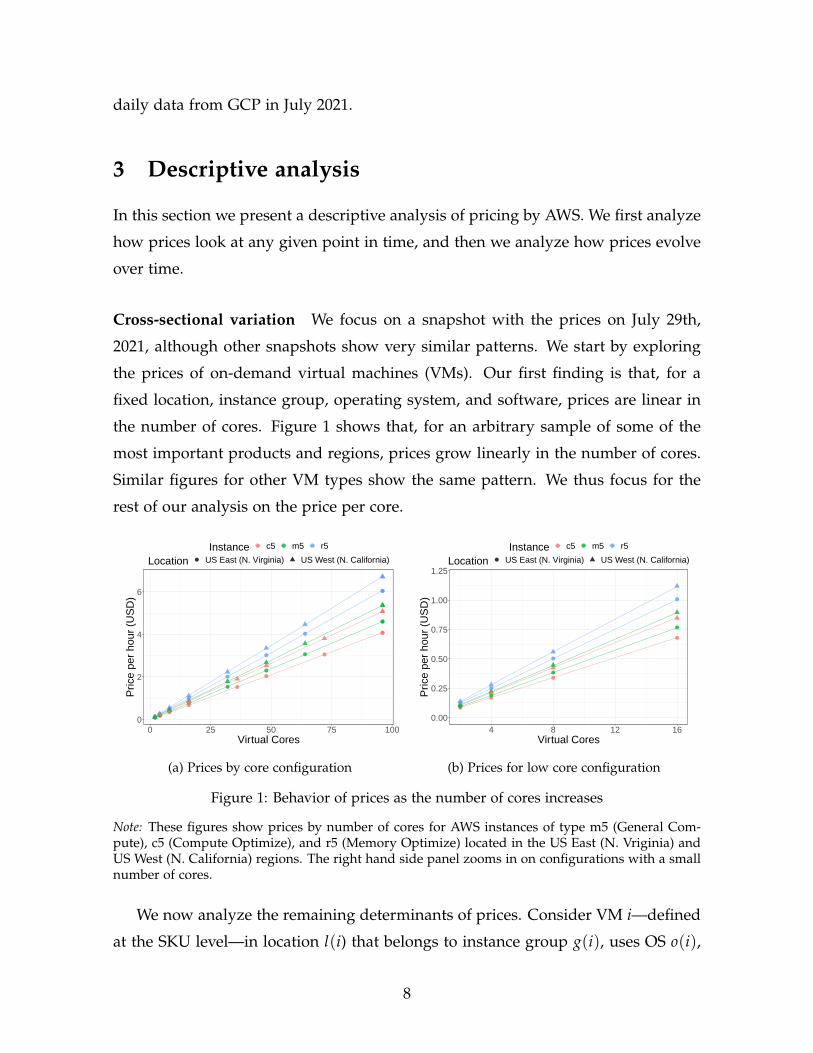
Cross-sectional variation We focus on a snapshot with the prices on July 29th,
2021, although other snapshots show very similar patterns. We start by exploring
the prices of on-demand virtual machines (VMs). Our first finding is that, for a
fixed location, instance group, operating system, and software, prices are linear in
the number of cores. Figure 1 shows that, for an arbitrary sample of some of the
most important products and regions, prices grow linearly in the number of cores.
Similar figures for other VM types show the same pattern. We thus focus for the
rest of our analysis on the price per core.
0
2
4
6
0 25 50 75 100Virtual Cores
Pric
e pe
r ho
ur (
US
D)
Instance c5 m5 r5
Location US East (N. Virginia) US West (N. California)
(a) Prices by core configuration
0.00
0.25
0.50
0.75
1.00
1.25
4 8 12 16Virtual Cores
Pric
e pe
r ho
ur (
US
D)
Instance c5 m5 r5
Location US East (N. Virginia) US West (N. California)
(b) Prices for low core configuration
Figure 1: Behavior of prices as the number of cores increases
Note: These figures show prices by number of cores for AWS instances of type m5 (General Com-pute), c5 (Compute Optimize), and r5 (Memory Optimize) located in the US East (N. Vriginia) andUS West (N. California) regions. The right hand side panel zooms in on configurations with a smallnumber of cores.
We now analyze the remaining determinants of prices. Consider VM i—defined
at the SKU level—in location l(i) that belongs to instance group g(i), uses OS o(i),
8
is of tenancy τ(i) (whether the VM is in a fixed pysical server or AWS has the
flexibility to choose it), and uses software s(i). These five dimensions account for
essentially all the remaining variation in prices. A regression of log price per core
on the interaction of fixed effects for these five dimensions has an R2 of 0.953, and
of 0.970 if we focus on the most important products. We then decompose price
variation across these four dimensions by running a regression of the form
log(pi) = αl(i) + βg(i) + γo(i) + δs(i) + ητ(i) + εi, (1)
where pi is the price per core and the first five terms represent fixed effects at the
location, instance group, OS, software and tenancy level.
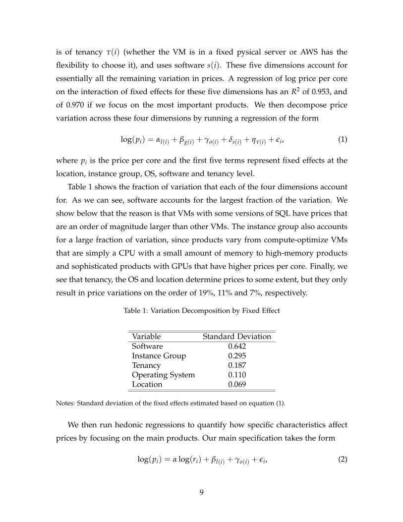
Table 1 shows the fraction of variation that each of the four dimensions account
for. As we can see, software accounts for the largest fraction of the variation. We
show below that the reason is that VMs with some versions of SQL have prices that
are an order of magnitude larger than other VMs. The instance group also accounts
for a large fraction of variation, since products vary from compute-optimize VMs
that are simply a CPU with a small amount of memory to high-memory products
and sophisticated products with GPUs that have higher prices per core. Finally, we
see that tenancy, the OS and location determine prices to some extent, but they only
result in price variations on the order of 19%, 11% and 7%, respectively.
Table 1: Variation Decomposition by Fixed Effect
Variable Standard DeviationSoftware 0.642Instance Group 0.295Tenancy 0.187Operating System 0.110Location 0.069
Notes: Standard deviation of the fixed effects estimated based on equation (1).
We then run hedonic regressions to quantify how specific characteristics affect
prices by focusing on the main products. Our main specification takes the form
log(pi) = α log(ri) + βl(i) + γo(i) + εi, (2)
9
0.0
0.2
0.4
0.6
Fix
ed E
ffect
Asia Europe N. America Rest of World
AWS Local Zone AWS Region AWS Wavelength Zone
(a) Location
0.0
0.1
0.2
0.3
0.4
Linux RHEL RHEL w/ HA SUSE Windows
Fix
ed E
ffect
(b) Operative System
Figure 2: Estimate Fixed Effects by VM dimension
Note: These figures show estimated fixed effects according to equation (1). All estimated coefficientshave a p-value lower than 10−4. The reference category for location is the Asia Pacific (Mumbai)region. The "Rest of the world" category in subfigure (a) is composed of the Cape Town and SaoPaulo AWS regions.
where ri represents the RAM memory per core. We obtain an estimate α̂ = 0.249
(s.e.=0.003), which implies that increasing the RAM memory by 10% leads to a
price increase of 2.5%. Figure 2 plots the values of the fixed effects coefficients. We
can see how certain versions of SQL lead to prices that are an order of magnitude
higher than VMs without specialized software. VMs with Windows, SUSE, and Red
Hat Linux (RHEL) are more expensive by 15%-45% than VMs that use free Linux
distributions. Finally, we observe that locations defined at the local-zone level are
more expensive than those that are defined at the region level (typically by 38%),
and wavelength-zone locations are more expensive by 44%.
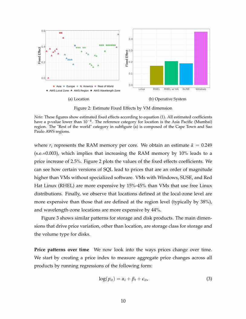
Figure 3 shows similar patterns for storage and disk products. The main dimen-
sions that drive price variation, other than location, are storage class for storage and
the volume type for disks.
Price patterns over time We now look into the ways prices change over time.
We start by creating a price index to measure aggregate price changes across all
products by running regressions of the following form:
log(pit) = αi + βt + εit, (3)
10
0.0
0.5
1.0
1.5
2.0
Cold HDD Gen. Purpose Magnetic Prov. IOPS St1−HDD
Fix
ed E
ffect
(a) Disks Volume Type
0.0
0.5
1.0
1.5
Archive Gen. Purpose Infreq. Access Non−Critical
Fix
ed E
ffect
(b) Storage Class
Figure 3: Estimated Fixed Effects for AWS storage and disks
Note: These figures show estimated fixed effects for AWS disks and storage. All estimated coeffi-cients have a p-value lower than 10−4. Subfigure (a) shows the volume type fixed effects. GeneralPurpose and Provisioned IOPS are Solid State Drives; Cold HDD, Magnetic and Throughtput Opti-mized HDD (st1-HDD) are Hard Disk Drives. The storage class Archive in subfigure (b) correspondto AWS Glacier, a low-availability product.
where pit is the price per core at time t for product i (again, defined at the SKU
level), αi is a fixed effect at the SKU level, and βt is a time period fixed effect. We
then use our estimate for βt as a measure of overall price levels.
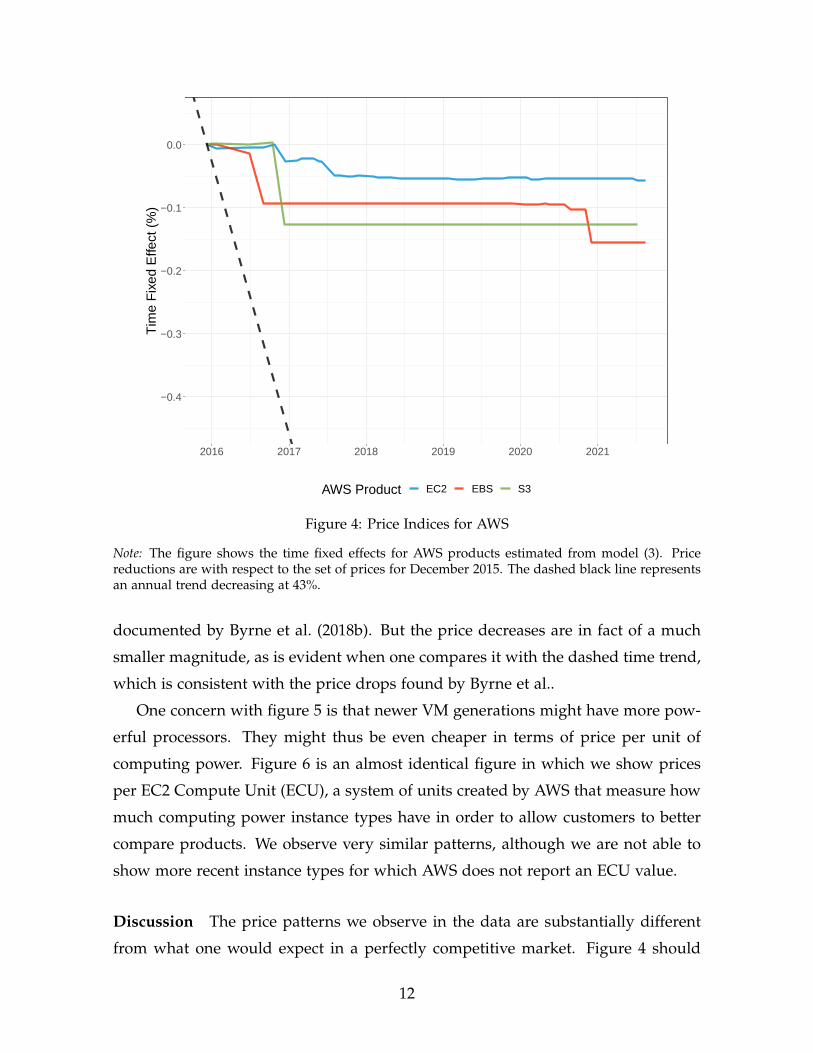
Figure (4) plots the price indices we construct for virtual machines, storage, and
disk, using the first period as the base level. We see that prices mostly remain
constant, except for a few periods during which prices go down. For comparison,
the dashed line shows how prices would have behaved if they followed the price
trend for semiconductors measured by Byrne et al. (2018b) for 2008-2013—i.e., a
price drop of 43% per year. The aggregate price decrease is nowhere near what
one would expect if prices followed the same trend as CPU prices—which roughly
follow Moore’s law.
In order to get a better understanding of the price changes shown by this figure,
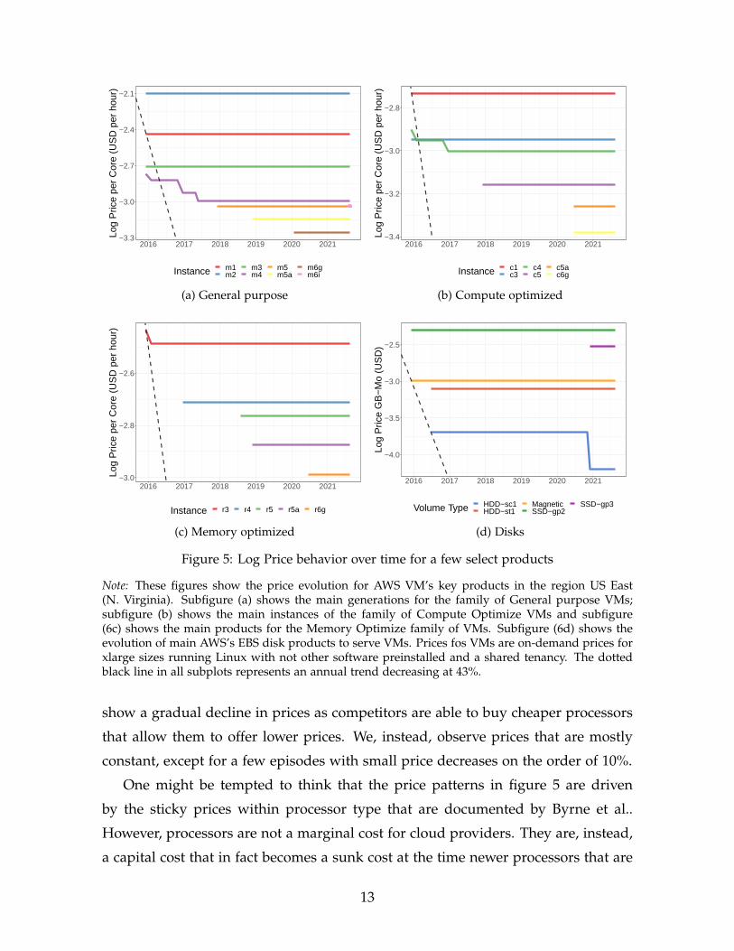
we now focus on the behavior of the prices of a few key products. Figure 5 plots
the log prices of general-purpose, compute optimized, and memory optimized VMs
located in North Virginia.4 Prices almost never change. The most important pattern
is that new generations are introduced at a lower price than the previous generation.
This pattern is consistent with the pricing scheme followed by Intel since 2010, as
4Figures for other locations are almost identical.
11
−0.4
−0.3
−0.2
−0.1
0.0
2016 2017 2018 2019 2020 2021
Tim
e F
ixed
Effe
ct (
%)
AWS Product EC2 EBS S3
Figure 4: Price Indices for AWS
Note: The figure shows the time fixed effects for AWS products estimated from model (3). Pricereductions are with respect to the set of prices for December 2015. The dashed black line representsan annual trend decreasing at 43%.
documented by Byrne et al. (2018b). But the price decreases are in fact of a much
smaller magnitude, as is evident when one compares it with the dashed time trend,
which is consistent with the price drops found by Byrne et al..
One concern with figure 5 is that newer VM generations might have more pow-
erful processors. They might thus be even cheaper in terms of price per unit of
computing power. Figure 6 is an almost identical figure in which we show prices
per EC2 Compute Unit (ECU), a system of units created by AWS that measure how
much computing power instance types have in order to allow customers to better
compare products. We observe very similar patterns, although we are not able to
show more recent instance types for which AWS does not report an ECU value.
Discussion The price patterns we observe in the data are substantially different
from what one would expect in a perfectly competitive market. Figure 4 should
12
−3.3
−3.0
−2.7
−2.4
−2.1
2016 2017 2018 2019 2020 2021
Log
Pric
e pe
r C
ore
(US
D p
er h
our)
Instance m1m2
m3m4
m5m5a
m6gm6i
(a) General purpose
−3.4
−3.2
−3.0
−2.8
2016 2017 2018 2019 2020 2021
Log
Pric
e pe
r C
ore
(US
D p
er h
our)
Instance c1c3
c4c5
c5ac6g
(b) Compute optimized
−3.0
−2.8
−2.6
2016 2017 2018 2019 2020 2021
Log
Pric
e pe
r C
ore
(US
D p
er h
our)
Instance r3 r4 r5 r5a r6g
(c) Memory optimized
−4.0
−3.5
−3.0
−2.5
2016 2017 2018 2019 2020 2021
Log
Pric
e G
B−
Mo
(US
D)
Volume Type HDD−sc1HDD−st1
MagneticSSD−gp2
SSD−gp3
(d) Disks
Figure 5: Log Price behavior over time for a few select products
Note: These figures show the price evolution for AWS VM’s key products in the region US East(N. Virginia). Subfigure (a) shows the main generations for the family of General purpose VMs;subfigure (b) shows the main instances of the family of Compute Optimize VMs and subfigure(6c) shows the main products for the Memory Optimize family of VMs. Subfigure (6d) shows theevolution of main AWS’s EBS disk products to serve VMs. Prices fos VMs are on-demand prices forxlarge sizes running Linux with not other software preinstalled and a shared tenancy. The dottedblack line in all subplots represents an annual trend decreasing at 43%.
show a gradual decline in prices as competitors are able to buy cheaper processors
that allow them to offer lower prices. We, instead, observe prices that are mostly
constant, except for a few episodes with small price decreases on the order of 10%.
One might be tempted to think that the price patterns in figure 5 are driven
by the sticky prices within processor type that are documented by Byrne et al..
However, processors are not a marginal cost for cloud providers. They are, instead,
a capital cost that in fact becomes a sunk cost at the time newer processors that are
13

−1.6
−1.4
−1.2
2016 2017 2018 2019 2020 2021
Log
Pric
e pe
r E
CU
(U
SD
per
hou
r)
Instance m1 m2 m3 m4 m5
(a) General purpose
−1.8
−1.5
−1.2
−0.9
−0.6
2016 2017 2018 2019 2020 2021
Log
Pric
e pe
r E
CU
(U
SD
per
hou
r)
Instance c1 c3 c4 c5
(b) Compute optimized
−1.3
−1.2
−1.1
2016 2017 2018 2019 2020 2021
Log
Pric
e pe
r E
CU
(U
SD
per
hou
r)
Instance r3 r4 r5
(c) Memory optimized
−4.0
−3.5
−3.0
−2.5
2016 2017 2018 2019 2020 2021
Log
Pric
e G
B−
Mo
(US
D)
Volume Type HDD−sc1HDD−st1
MagneticSSD−gp2
SSD−gp3
(d) Disks
Figure 6: Price per ECU behavior over time for a few select products
Note: These figures show the price per ECU evolution for AWS VM’s key products in the regionUS East (N. Virginia). Subfigure (a) shows the main generations for the family of General purposeVMs; subfigure (b) shows the main instances of the family of Compute Optimize VMs and subfigure(6c) shows the main products for the Memory Optimize family of VMs. Subfigure (6d) shows theevolution of main AWS’s EBS disk products to serve VMs. Prices fos VMs are on-demand prices forxlarge sizes running Linux with not other software preinstalled and a shared tenancy. The dottedblack line in all subplots represents an annual trend decreasing at 43%.
both cheaper and more powerful are introduced. Thus, the fact that processor prices
do not change should not have an impact on the prices of old instance generations.
The question that remains is then: what kind of environment might induce
prices like those we observe in the data? One possibility is a setting in which
customers are locked in to a certain type of instance. That might occur if companies
design their systems in a way that only works with a very specific type of instance.
Another possibility is that customers are inattentive and therefore do not respond
14

as they should when new instance generations are introduced.
4 Model
We now present a model of the cloud market in order to formalize the ideas dis-
cussed in previous sections.
Demand Consider customer i, who wants to satisfy one unit of computing needs
at time t in location l. If he chooses product j from provider k, he obtains utility
ultikj = αpltkj + βixltkj − γ1(yl,t−1,i 6= kj)− λ1(yl,t−1,i /∈ Jk) + ξltkj + εltikj, (4)
where pltj is the price of product j at time t in location l and xltj is a vector of product
characteristics (including the type of processor, the amount and type of memory,
and any additional features such as GPUs or higher disk throughput). The variable
ylti represents the product chosen by consumer i during the previous period, and Jk
represents the set of all VMs offered by provider k. The term γ1(yl,t−1,i 6= kj) thus
represents a cost of switching VM types and δ1(yl,t−1,i /∈ Jk) represents a cost of
switching providers. Finally, ξltj represents a product-market unobservable term.
In reality, corporate customers do not demand single units of computation. A
large company that relies on cloud computing, such as Airbnb, demands a large
number of computation units. In practice, we treat such companies as a large num-
ber of customers that use computing services on behalf of the company, each one
of which has different tastes.
With this specification for utility, and if we assume the error term εltij is dis-
tributed iid extreme value type I, the market share for product jk in market lt is
given by
σltkj =exp(δltkj)
∑k′ j′ exp(δltk′ j′), (5)
where δltkj = αpltkj + βixltkj − γ1(yl,t−1,i 6= kj)− λ1(yl,t−1,i /∈ Jk) + ξltkj. If we define
Qlt to be the total market size in location l at time t, then the demand for product
jk in market lt is given by qltkj = σltkjQlt.
15
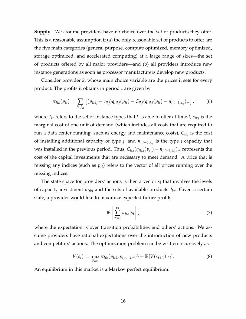
Supply We assume providers have no choice over the set of products they offer.
This is a reasonable assumption if (a) the only reasonable set of products to offer are
the five main categories (general purpose, compute optimized, memory optimized,
storage optimized, and accelerated computing) at a large range of sizes—the set
of products offered by all major providers—and (b) all providers introduce new
instance generations as soon as processor manufacturers develop new products.
Consider provider k, whose main choice variable are the prices it sets for every
product. The profits it obtains in period t are given by
πltk(plt) = ∑j∈Jkt
[(pltkj − clkj)qltkj(plt)− Clkj(qltkj(plt)− nl,t−1,k,j)+
], (6)
where Jkt refers to the set of instance types that k is able to offer at time t, clkj is the
marginal cost of one unit of demand (which includes all costs that are required to
run a data center running, such as energy and maintenance costs), Clkj is the cost
of installing additional capacity of type j, and nl,t−1,k,j is the type j capacity that
was installed in the previous period. Thus, Clkj(qltkj(plt)− nl,t−1,k,j)+ represents the
cost of the capital investments that are necessary to meet demand. A price that is
missing any indices (such as plt) refers to the vector of all prices running over the
missing indices.
The state space for providers’ actions is then a vector st that involves the levels
of capacity investment nltkj and the sets of available products Jkt. Given a certain
state, a provider would like to maximize expected future profits
E
[∞
∑τ=t
πltk
∣∣∣st
], (7)
where the expectation is over transition probabilities and others’ actions. We as-
sume providers have rational expectations over the introduction of new products
and competitors’ actions. The optimization problem can be written recursively as
V(st) = maxpltk
πltk(pltk, pl,t,−k; st) + E[V(st+1)|st]. (8)
An equilibrium in this market is a Markov perfect equilibrium.
16

Future steps The next step will be to use our data to estimate the main model
parameters. The main variation we will use in order to estimate demand is the
introduction of new products. We will use various sources of data in order to back
out the marginal and capital costs of cloud providers.
After having estimated the model, we can then measure welfare across different
counterfactuals. The first counterfactual is an approximation of a perfectly compet-
itive market where we introduce a large number of competitors. By comparing this
counterfactual to the status quo we can quantity the welfare losses due to a lack
of competition in this market. We can also simulate intermediate counterfactuals
in which a limited number of competitors enter in order to asses how large are
the barriers to entry. Finally, we can also run counterfactuals in which the current
cloud providers merge in order to assess how large are the potential welfare losses
if regulators allowed the market to turn into a monopoly.
5 Conclusions
With the goal of measuring the degree of competitiveness in the cloud industry,
we collected a dataset with historic prices of AWS, the largest cloud provider. A
descriptive analysis reveals many patterns that one would not observe in a perfectly
competitive market, suggesting a low degree of competition in this market. We will
complement our data with prices from the other two major cloud providers, as well
as a dataset with transactions for Microsoft Azure. We will use that data to estimate
a structural model of the cloud computing market, which will allow us to quantify
the welfare effects of a lack of competition.
References
Berry, Steven, James Levinsohn, and Ariel Pakes, “Automobile Prices in Market
Equilibrium,” Econometrica, 1995, 63 (4), 841–890.
Bloom, Nicholas, Tarek Alexander Hassan, Aakash Kalyani, Josh Lerner, and
Ahmed Tahoun, “The Diffusion of Disruptive Technologies,” Working paper, 2021.
17
Blumenthal, Marjory S, “Is security lost in the clouds?,” Communications and Strate-
gies, 2011, (81), 69–86.
Bresnahan, Timothy and Pai-Ling Yin, “Adoption of new information and commu-
nications technologies in the workplace today,” Innovation policy and the economy,
2017, 17 (1), 95–124.
Brynjolfsson, Erik, Daniel Rock, and Chad Syverson, Artificial Intelligence and the
Modern Productivity Paradox: A Clash of Expectations and Statistics, University of
Chicago Press, 2019.
Byrne, D and C Corrado, “ICT Prices and ICT Services: What do they tell us about
Productivity and Technology? Washington. Board of Governors of the Federal
Reserve System,” Working Paper, 2017.
Byrne, David, Carol Corrado, and Daniel E Sichel, “The rise of cloud computing:
minding your P’s, Q’s and K’s,” Working paper, 2018.
Byrne, David M, Stephen D Oliner, and Daniel E Sichel, “How fast are semicon-
ductor prices falling?,” Review of Income and Wealth, 2018, 64 (3), 679–702.
Determann, Lothar and David Nimmer, “Software Copyright’s Oracle from the
Cloud,” Berkeley Tech. LJ, 2015, 30, 161.
Flamm, Kenneth, “Measuring Moore’s law: evidence from price, cost, and quality
indexes,” Working paper, 2018.
Gartner, “Gartner Forecasts Worldwide Public Cloud End-User Spending to Grow
23% in 2021,” [Press release] 2021. Click here to open URL.
Gorodnichenko, Yuriy, Oleksandr Talavera, and Nam Vu, “Quality and price set-
ting of high-tech goods,” Economic Modelling, 2021, 98, 69–85.
Jin, Wang and Kristina McElheran, “Economies before scale: survival and perfor-
mance of young plants in the age of cloud computing,” Working paper, 2017.
Kannan, Aadharsh, Jacob LaRiviere, and R Preston McAfee, “Characterizing the
Usage Intensity of Public Cloud,” ACM Transactions on Economics and Computation
(TEAC), 2021, 9 (3), 1–18.
Kilcioglu, Cinar, Justin M Rao, Aadharsh Kannan, and R Preston McAfee, “Usage
patterns and the economics of the public cloud,” in “Proceedings of the 26th
International Conference on World Wide Web” 2017, pp. 83–91.
Nosko, Chris, “Competition and quality choice in the cpu market,” Working paper,
18
2010.
Renda, Andrea, “Competition, neutrality and diversity in the cloud,” Communica-
tions & Strategies, 2012, (85), 23–44.
Seddon, Jonathan J.M. and Wendy L. Currie, “Cloud computing and trans-border
health data: Unpacking U.S. and EU healthcare regulation and compliance,”
Health Policy and Technology, 2013, 2 (4), 229–241.
Su, Jeb, “Amazon Owns Nearly Half Of The Public-Cloud Infrastructure Market
Worth Over $32 Billion: Report,” Forbes, 2021. Click here to open URL.
Wang, Shuang, Jacob LaRiviere, and Aadharsh Kannan, “Spatial competition and
missing data: An application to cloud computing,” Working paper, 2020.
Yoo, Christopher S. and Jean-Francois Blanchette, eds, Regulating the cloud: Policy
for computing infrastructure, MIT Press, 2015.
19