competing mechanisms in strongly correlated systems …people.sissa.it/~becca/theses/ferrero.pdf ·...
TRANSCRIPT

SISSA Scu
ola
Inter
nazionale Superiore di Studi Avanzati
- ma per seguir virtute e conoscenza
-
ISAS
INTERNATIONAL SCHOOL FOR ADVANCED STUDIESCondensed Matter Sector
Competing Mechanisms in Strongly
Correlated Systems Close to a
Mott Insulator
Thesis submitted for the degree of
Doctor Philosophiæ
Candidate
Michel Ferrero
Supervisors
Prof. Michele Fabrizio
Dr Federico Becca
October 2006


Contents
Contents i
Acknowledgments iii
1 Introduction 1
2 The Mott Transition: Models and Methods 9
2.1 The Hubbard Model . . . . . . . . . . . . . . . . . . . . . . . 9
2.2 Gutzwiller Wave Functions . . . . . . . . . . . . . . . . . . . 10
2.2.1 Original Formulation . . . . . . . . . . . . . . . . . . 11
2.2.2 A Word About the d →∞ Limit . . . . . . . . . . . . 132.2.3 Generalized Multi-Band Gutzwiller Wave Functions . . 14
2.2.4 Example: The Single-Band Hubbard Model . . . . . . 18
2.3 Dynamical Mean-Field Theory . . . . . . . . . . . . . . . . . 19
2.3.1 Mapping to a Single-Site Model . . . . . . . . . . . . 20
2.3.2 The d →∞ Limit . . . . . . . . . . . . . . . . . . . 222.3.3 The Bethe Lattice . . . . . . . . . . . . . . . . . . . 24
2.3.4 Implementation by Iteration . . . . . . . . . . . . . . 25
2.4 The Anderson Impurity Model . . . . . . . . . . . . . . . . . 26
2.5 The Kondo Model . . . . . . . . . . . . . . . . . . . . . . . . 30
2.6 Wilson’s Numerical Renormalization Group . . . . . . . . . . 32
2.6.1 One-Dimensional Formulation of the Model . . . . . . 33
2.6.2 Logarithmic Discretization . . . . . . . . . . . . . . . 34
2.6.3 Iterative Diagonalization . . . . . . . . . . . . . . . . 36
2.6.4 Implementation . . . . . . . . . . . . . . . . . . . . . 37
2.6.5 Fixed Points . . . . . . . . . . . . . . . . . . . . . . . 37
2.6.6 Spectral Function . . . . . . . . . . . . . . . . . . . . 38
2.7 Conformal Field Theory . . . . . . . . . . . . . . . . . . . . . 39
2.7.1 Boundary Conformal Field Theory . . . . . . . . . . . 40
2.7.2 Ground-State Degeneracy . . . . . . . . . . . . . . . 44
2.7.3 Scattering Matrix . . . . . . . . . . . . . . . . . . . . 44
i

ii Contents
3 Different Bandwidths in the Two-Band Hubbard Model 47
3.1 Introduction . . . . . . . . . . . . . . . . . . . . . . . . . . . 47
3.2 The Model . . . . . . . . . . . . . . . . . . . . . . . . . . . . 49
3.3 Gutzwiller Variational Technique . . . . . . . . . . . . . . . . 50
3.3.1 Results for J = 0 . . . . . . . . . . . . . . . . . . . . 52
3.3.2 Results for J 6= 0 . . . . . . . . . . . . . . . . . . . . 553.4 Dynamical Mean-Field Theory . . . . . . . . . . . . . . . . . 57
3.5 Single Impurity Spectral Properties . . . . . . . . . . . . . . . 63
3.6 Projective Self-Consistent Technique . . . . . . . . . . . . . . 65
3.7 Discussion and Conclusions . . . . . . . . . . . . . . . . . . . 69
4 Critical Behavior in Impurity Trimers and Tetramers 73
4.1 Introduction . . . . . . . . . . . . . . . . . . . . . . . . . . . 73
4.2 The Impurity Dimer . . . . . . . . . . . . . . . . . . . . . . . 77
4.3 The Impurity Trimer . . . . . . . . . . . . . . . . . . . . . . 80
4.3.1 CFT Preliminaries for the Trimer . . . . . . . . . . . 81
4.3.2 Fixed Points in the Trimer Phase Diagram . . . . . . 82
4.3.3 Concluding Remarks About the Trimer . . . . . . . . 90
4.4 The Impurity Tetramer . . . . . . . . . . . . . . . . . . . . . 91
4.4.1 CFT Preliminaries for the Tetramer . . . . . . . . . . 92
4.4.2 Fixed Points in the Tetramer Phase Diagram . . . . . 93
4.5 Conclusions . . . . . . . . . . . . . . . . . . . . . . . . . . . 99
A Character Decompositions 101
A.1 The Impurity Trimer . . . . . . . . . . . . . . . . . . . . . . 101
A.2 The Impurity Tetramer . . . . . . . . . . . . . . . . . . . . . 102
B Modular S-Matrices 105
B.1 Modular S-Matrix for the Ising Model . . . . . . . . . . . . . 105B.2 Modular S-Matrix for the TIM . . . . . . . . . . . . . . . . . 105
B.3 Modular S-Matrix for the c = 1 CFT . . . . . . . . . . . . . 106
Bibliography 107

Acknowledgments
I would like to express my gratitude to Michele Fabrizio for proposing the
challenging and exciting subjects of my thesis and for sharing his enthusiasm,
understanding and profound knowledge of the theory of strongly correlated
systems. My sincere thanks also to Federico Becca for helping and assisting
me with great expertise, for his encouragements and availability. The close
cooperation and numerous discussions with Michele and Federico have been a
continuous motivation as well as a most rewarding experience for me.
Many thanks also to Frederic Mila for introducing me to the field of con-
densed matter physics at the EPFL in Lausanne and for remaining available
and open to communication during my years in Trieste. It has been a fantastic
opportunity to be able to continue working together with him and with Arnaud
Ralko, Federico Becca and Dmitri Ivanov on the project of quantum dimers.
I am grateful to my friends of the condensed matter group at the EPFL for
their hospitality and the many fruitful exchanges, especially with Arnaud Ralko
and Cedric Weber.
The work related to the orbital-selective Mott transition has been enhanced
by many instructive debates with Massimo Capone, Luca de’ Medici, Antoine
Georges, Akihisa Koga, Ansgar Liebsch, Nicola Manini, and Manfred Sigrist. I
am obliged to all of them. I am also indebted to Lorenzo de Leo and Giuseppe
Santoro for introducing me to Wilson’s numerical renormalization group.
It has been a pleasure to spend these fascinating years at SISSA together
with many new friends, sharing our scientific and other interests. In this re-
spect, I wish to acknowledge the captivating conversations with Walter van
Suijlekom, Guido Fratesi, Adriano Mosca Conte, Manuela Capello, Tommaso
Caneva and Nicola Lanata. I would also like to thank Giuliano Niccoli for our
lasting friendship and for the help he gave me in understanding certain aspects
of conformal field theory.
Finally, I would like to thank my family for the support they provided me
and for their continuous encouragements and trust as well as Petra for the
wonderful time we have spent together in Trieste.
iii


Chapter 1
Introduction
Strongly Correlated Systems
One of the greatest successes of the quantum mechanical description of solids
certainly was the development of band structure theory and the classification
of crystalline solids into conductors and insulators. Roughly speaking, within
this approach every electron is assumed to feel an effective periodic potential
produced by the positive ions and the other electrons, and any other electron-
electron correlation is neglected. The eigenstates of the one-particle prob-
lem are classified according to their crystal momentum and the corresponding
eigenvalues form dispersing bands. If the number of electrons in the crystal is
such that there is a finite energy gap between the last occupied state and the
lowest unoccupied one, the crystal is an insulator, otherwise it is a metal.
Even if this treatment seems oversimplified, it has been very successful,
especially to describe solids with very wide bands. However, soon after the
introduction of band theory, examples were shown that could not be under-
stood within this framework. In 1934, de Boer and Verwey [19] reported that
many properties of some transition-metal oxides were in disagreement with
band-structure calculations. These materials are insulators whereas they are
expected to be conductors because of their partially filled d-band. Mott and
Peierls [92, 93] suggested that the reason for the failure of conventional band
structure theory might be its poor mean-field-like treatment of the repulsive
electron-electron Coulomb interaction. Indeed, if the electrons were moving
slowly, they would be spending more time on every atomic site and hence expe-
rience a strong interaction with the other electrons present on the same atom.
If the energy cost of this interaction is too big, it might become favorable for
the electrons to stop moving at all and form what is now universally called a
Mott insulator.
With these considerations, the solids can be further classified. In those with
large conduction bands, the electrons are delocalized and move fast over the
whole crystal. They do not interact strongly and are well described by Bloch
1

2 Introduction
waves. Other solids, instead, have narrower bands with the consequence that
the electrons move slower and remain for a longer time at a given lattice site.
Typical candidates are transition metal oxides where the hopping between the
partially filled d-shells of the transition metal ions is bridged by the oxygen cage
and can hence become comparable with the d-shell Coulomb repulsion or the
metal-oxygen charge transfer gap. Other candidates are for instance molecular
conductors, where the large separation between neighboring molecules makes
the inter-molecular hopping very small. As a result, the energy scale coming
from the electronic interaction becomes of the same order as the band energy
gain. These systems are said to be strongly correlated and the rather localized
electrons are not anymore well characterized by the purely Bloch wave-like
picture provided by band theory. In some cases, correlations are so strong to
stabilize a Mott insulator where a description in terms of localized Wannier
orbitals is the most appropriate. In less extreme situations, the correlated
material is still metallic but the competition between the two energy scales,
and hence between a wave-like against a particle-like behavior, leads to very
interesting physical phenomena.
Over the past decades, many novel materials displaying unusual behaviors
that are poorly described by conventional techniques have been discovered
and together with these, new theoretical methods have been developed. The
behavior of magnetic impurities diluted in a metallic host and the subsequent
introduction of the Kondo and Anderson impurity models are just one example
of these phenomena. It is however surely the discovery of high-temperature
superconductivity [16] in doped Mott insulator cuprates that triggered today’s
great interest in strongly correlated materials.
Experimental Results
Let us consider some particular examples where strong electronic correlations
play a relevant role. A very interesting experimental opportunity arises when
it is possible to control the bandwidth by varying external parameters, like the
pressure, that modify the structure of the crystal and increase or decrease the
overlap between neighboring orbitals. For some materials, it is then possible
to induce a Mott transition from a metal to a Mott insulator, or vice versa,
as a function of external parameters. This is the case for (V1−xCrx)2O3 [83]
whose phase diagram is shown in the left panel of Fig. 1.1. At temperatures
above ∼ 200 K a Mott transition between a paramagnetic insulator and ametal is observed. It is interesting to note that, at low temperatures, the
insulator develops an antiferromagnetic ordering, signaling that other energy
scales besides the Coulomb repulsion/charge transfer gap and the band energy
gain, come into play: in this example, the Coulomb exchange, the super-
exchange and the coupling to the lattice.
Another example is the organic compound κ-(BEDT-TTF)2Cu[N(CN)2]Cl

Introduction 3
Figure 1.1: Left: Phase diagram for the metal-insulator transi-
tion in (V1−xCrx)2O3 as a function of doping with Cr or Ti and
as a function of pressure [83]. Right: Phase diagram of κ-(BEDT-
TTF)2Cu[N(CN)2]Cl as a function of pressure [76].
showing unconventional superconductivity at low temperatures. Its phase di-
agram [76] is shown in the right panel of Fig. 1.1. An observation strikes
the eye: There are many similarities between this phase diagram and that
of (V1−xCrx)2O3 although the energy scales are very different. This sug-
gests that the mechanisms behind the Mott transition have a universal char-
acter. Here too, the paramagnetic insulator becomes magnetically ordered
below ∼ 20 K.Signals of strong correlations are also found in the spectroscopic properties
of many compounds. In Fig. 1.2 (left panel) we show the photoemission
spectra for several d1 transition metal oxides. In these systems, the lattice
distortion changes the overlap between neighboring d-orbitals such that the
compounds range from a Mott insulator to a paramagnetic metal [39]. It is
clear from the data that the lower band seen at ∼ −1.5 eV (called the lowerHubbard band) in the insulating YTiO3 is already preformed in the metallic
phase, e.g. of SrVO3. Such a feature is not at all captured by standard band-
structure calculations. In the metallic phase there is also a visible separation
between a quasiparticle peak and the Hubbard band as one gets closer to the
Mott transition. Although in this early data the the quasiparticle peak is not
very visible, later experiments allowed to have a higher definition, as shown in
the right panel of Fig. 1.2. In this experiment [89], the photoemission spectra is
shown for different photon energies. When the latter increases, thus sampling
the solid deeper in the bulk, the quasiparticle peak gets higher and sharper.

4 Introduction
Inte
nsity
(arb
. uni
t)
-3.0 -2.5 -2.0 -1.5 -1.0 -0.5 0.0 0.5
E-EF(eV)
ab
c
d
e
a: hν=700eVb: hν=500eVc: k-averagedd: hν=310eVe: Schramme et al. hν=60eV
Figure 1.2: Left: Photoemission spectra of different perovskite-type
transition metal oxides in the d-band region [39]. Right: Photoemis-
sion spectra of V2O3 taken with various photon energies hν [89].
Let us finally show some experimental results about the single-layered
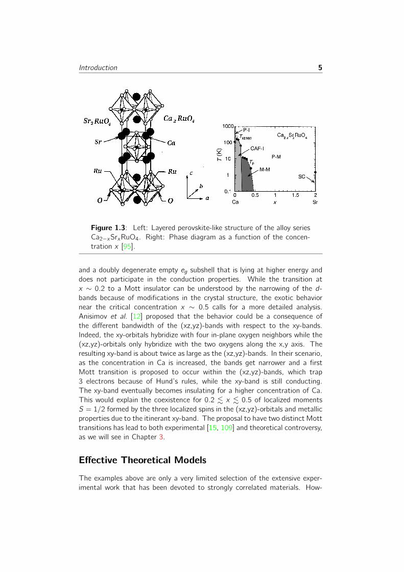
ruthenates Ca2−xSrxRuO4 that are pertinent to the study of Chapter 3. The
basic crystal structure of this compound is shown in the left panel of Fig. 1.3.
The ruthenates have lately attracted a lot of interest because of the uncon-
ventional spin-triplet superconductivity observed in Sr2RuO4 [80]. Curiously,
while Sr2RuO4 is a well-defined Fermi liquid, the substitution of Ca2+ for Sr2+
produces a Mott insulator, Ca2RuO4, with a staggered moment S = 1. Be-
tween these two extremes [95], a series of correlated metallic states are found,
see the phase diagram in Fig. 1.3 (right panel). At low temperature, for dop-
ings 0.5 . x < 2, the system is a paramagnetic metal. As x → 0.5, thecharacteristic Curie-Weiss temperature approaches zero. The most unusual
properties are found at the critical concentration x = 0.5, where the magnetic
susceptibility shows a free Curie form with a spin S = 1/2, coexisting with
metallic transport properties. The region 0.2 . x . 0.5 is characterized byantiferromagnetic correlations, still coexisting with metallic properties. Finally,
for Ca concentrations x . 0.2, an insulating behavior is stabilized.
In these ruthenate alloys, the relevant 4d-orbitals are split by the crystal
field into an essentially threefold degenerate t2g subshell that hosts 4 electrons
Introduction 5
Figure 1.3: Left: Layered perovskite-like structure of the alloy series
Ca2−xSrxRuO4. Right: Phase diagram as a function of the concen-
tration x [95].
and a doubly degenerate empty eg subshell that is lying at higher energy and
does not participate in the conduction properties. While the transition at
x ∼ 0.2 to a Mott insulator can be understood by the narrowing of the d-bands because of modifications in the crystal structure, the exotic behavior
near the critical concentration x ∼ 0.5 calls for a more detailed analysis.Anisimov et al. [12] proposed that the behavior could be a consequence of
the different bandwidth of the (xz,yz)-bands with respect to the xy-bands.
Indeed, the xy-orbitals hybridize with four in-plane oxygen neighbors while the
(xz,yz)-orbitals only hybridize with the two oxygens along the x,y axis. The
resulting xy-band is about twice as large as the (xz,yz)-bands. In their scenario,
as the concentration in Ca is increased, the bands get narrower and a first
Mott transition is proposed to occur within the (xz,yz)-bands, which trap
3 electrons because of Hund’s rules, while the xy-band is still conducting.
The xy-band eventually becomes insulating for a higher concentration of Ca.
This would explain the coexistence for 0.2 . x . 0.5 of localized momentsS = 1/2 formed by the three localized spins in the (xz,yz)-orbitals and metallic
properties due to the itinerant xy-band. The proposal to have two distinct Mott
transitions has lead to both experimental [15, 109] and theoretical controversy,
as we will see in Chapter 3.
Effective Theoretical Models
The examples above are only a very limited selection of the extensive exper-
imental work that has been devoted to strongly correlated materials. How-

6 Introduction
ever, they show features, like the coexistence of delocalized quasiparticles and
localized atomic-like excitations, or the presence of anomalous phases close
to a Mott transition, that are common to many other compounds. From a
theoretical standpoint, these similarities motivated the introduction of simple
and quite universal models designed such as to contain the minimum number
of ingredients able to uncover the physics of strong correlation. The most
known example is the single-band Hubbard model, which is believed to be rep-
resentative of many materials, including cuprates and the organic quasi-two
dimensional compounds of Fig. 1.1. In this model, a single valence orbital
per site is assumed. An electron on this orbital feels a Coulomb repulsion
from another electron sitting the same orbital. In addition, electrons can hop
from one lattice site to another. Even if very simplified, the Hubbard model
contains the main ingredient of strong correlation, namely the competition
between localization induced by the electronic repulsion and itineracy favored
by the hopping term. Since this competition arises when both the Coulomb
repulsion and the band-energy gain are comparable in magnitude, it lacks any
small expansion parameter and it is very difficult to study, even in the simple
case of the single-band Hubbard model. In spite of that, a lot of progresses
have been achieved thanks to the development of the so-called dynamical
mean-field theory [42]. Within this theory, a lattice model is mapped onto an
effective single-site problem, which amounts to assume that spatial fluctua-
tions are frozen, while full time dynamics is retained. This mapping is exact
in infinite coordination lattices, but yet, it is assumed to remain a sensible
approximation even beyond that limit. The resulting single-site model is easier
to study and intense analytical and numerical studies over the past 15 years
have shown that it captures many of the features observed experimentally. For
instance, this method allowed to show that the coexistence of delocalized and
localized single-particle excitations on well separated energy scales, as seen
in photoemission spectroscopy, is a generic feature of the above-mentioned
competition between the short-range Coulomb repulsion and the hopping en-
ergy. In other words, if one neglects all complications like magnetism or other
symmetry breakings that may intervene at very low temperature and only con-
siders the transition from a non-symmetry-breaking metal into an ideal non-
symmetry-breaking Mott insulator, this transition is indeed characterized by
the disappearance of a quasi-particle peak within well preformed Hubbard-side
bands, which are almost insensitive to the transition.
However, on the insulating side of the transition, new energy scales come
into play at low temperature, whose role is to rid the ideal non-symmetry-
breaking Mott insulator of its residual entropy. As a result, a realistic in-
sulating phase is eventually established, which is usually accompanied by a
phase transition into some symmetry-broken phase, for instance a magnetic-
ordered phase. These additional energy scales include, for instance, the on-site
Coulomb exchange, responsible for the Hund’s rules, the inter-site direct- or

Introduction 7
super-exchange, the coupling to the lattice or the crystal field. Obviously, these
processes do exist also in the metallic side of the transition, hence one may
wonder what is going to happen when the characteristic energy scale of the
quasiparticles becomes comparable with them. We are going to argue that this
situation uncovers a new type of competition which emerges before a metal-
to-insulator Mott transition and which is as generic as the main competition
between the Coulomb repulsion and the hopping energy.
The Thesis
In order to have further insight, let us assume that, among all these additional
low-energy scales, a single one dominates, denoted as J. It can be regarded
as the temperature at which the entropy of the residual degrees of freedom
of the ideal Mott insulator start to be quenched. This is in contrast to re-
cent research activities that focus on the possibility that different symmetry
broken phases may compete in the insulating phases, leading to exotic phe-
nomena [88]. We will discard this event and concentrate on the metallic phase
adjacent the Mott insulator. Here, the quenching of the entropy is due to the
formation of a Fermi sea of quasiparticles and takes place below the quasipar-
ticle effective Fermi temperature, T ∗F , which might be much smaller than the
bare TF due to strong correlations. Since Landau quasiparticles carry the same
quantum numbers as the electrons, the entropy quenching involves all degrees
of freedom at the same time, including the charge. However, the presence of
J provides the metallic phase with an alternative mechanism to freeze spin and
eventually orbital degrees of freedom, independently of the charge ones, and
becomes competitive with the onset of a degenerate quasiparticle gas when
T ∗F ' J. Unlike the competition between different symmetry-broken Mott-
insulating phases, which requires fine tuning of the Hamiltonian parameters
and may only accidentally occur in real materials, this new type of competition
should be accessible whenever it is possible to move gradually from a Mott
insulator into a metallic phase, for instance by doping or applying pressure.
Clearly, a single-site, single-band model is not suited to study this issue.
However, over the past years a large effort has been devoted to account for
these extra ingredients like the exchange-splitting, the crystal-field splitting,
the inter-site magnetic exchange and so on. They have for example lead to
multi-band generalizations or to extensions of the dynamical mean-field theory
that account for short-range spatial interactions by mapping the lattice model
onto a small cluster of sites. Nevertheless, most of these efforts have not
put much emphasis on the competition induced by these additional ingredi-
ents which, we believe, may be the key to understand the emergence of the
anomalous phases observed in many strongly-correlated materials close to a
Mott transition.
In this thesis, we intend to investigate the effects of this competition in

8 Introduction
two different generalizations of a single-band model. Let us briefly outline our
work:
In Chapter 2, we present some of the theoretical methods and models
that have been developed to study the physics of strongly correlated materials
and that will be used in the thesis. We follow the example of the single-
band Hubbard model for which the formalism is easiest to write, introducing
generalizations for some techniques when it proves necessary.
This will provide all the necessary background to investigate, in Chapter 3,
the role of the bandwidth difference in a two-band Hubbard model in infi-
nite dimensions. Such a model could be relevant to understand the physics
of compounds like the ruthenates described above. In particular, we explore
the possibility to have a so-called orbital-selective Mott transition, for which
distinct Mott transitions appear in the two bands at different values of the
on-site Coulomb repulsion. We show that for a ratio small enough between
the bandwidths, two distinct transitions can occur and that particular features
appear in the low-energy properties of the system.
In the second part of the thesis, presented in Chapter 4, we focus on the
properties of two clusters made of three and four impurities. These clusters
appear in extensions of the dynamical mean-field theory and we discuss them
in this context. We show that the competition between conventional Kondo
screening and inter-impurity couplings reveals a very interesting physics and
that the presence of anomalous bulk phases close to the Mott transition might
be traced back to instabilities that are already present at the impurity level.

Chapter 2
The Mott Transition: Modelsand Methods
We expose the main techniques that we use in Chapters 3 and 4. Even though
we will be investigating more complicated models, we consider the prototypical
example of the single-band Hubbard model and show the connection between
different methods that have been developed to understand its physics. The
first approach we introduce is the Gutzwiller variational technique and the so-
called Gutzwiller approximation to evaluate average values over the variational
wave function. We then present the dynamical mean-field theory, in which the
original Hubbard model is mapped onto a single-site problem, and emphasize
the important role played by impurity models to describe the Mott transition.
In particular, the Kondo and the Anderson impurity models are introduced as
well as Wilson’s numerical renormalization group that enables to study impurity
models in detail. We conclude the chapter with an overview of conformal
field theory, a powerful tool to analyze and classify the fixed points of the
renormalization group applied to impurity models.
2.1 The Hubbard Model
From a theoretical perspective, the search for an understanding of strongly
correlated systems has lead to the introduction of simplified models that cap-
ture the main features of strongly correlated electrons. Essentially simultane-
ously, Hubbard [54], Gutzwiller [45] and Kanamori [63] proposed a very simple
model that contains the minimum ingredients to account for both band-like
and localized behavior. Their model is obtained by neglecting fully-occupied
and unoccupied bands. It is more careful to say that the degrees of freedom
provided by these bands have been “integrated out”, leading to renormalized
parameters in the Hamiltonian. The remaining Wannier orbitals are those close
to the Fermi level (the valence bands) and, in the most elementary form of
the model, there is just one such orbital. This could represent materials in
9

10 The Mott Transition: Models and Methods
which the orbital degeneracy has been lifted completely by a crystal field. The
resulting Hamiltonian reads
H = H0 +Hint = −∑i jσ
ti j f†i ,σfj,σ +H.c.+ U
∑i
ni↑ni↓, (2.1)
where f †i ,σ creates an electron in the Wannier orbital with spin σ and niσ = f†iσfiσ
is the occupation number. The first part of the Hamiltonian H0 expresses,through ti j , the possibility of an electron hopping between neighboring sites i
and j . Another approximation is to neglect the long-range tail of the Coulomb
interaction which is assumed to be local. This is encoded in Hint and U is theenergy cost for having two electrons on the same orbital. Changing the ratio
U/t emulates the effect of varying external parameters like the pressure.
What makes the Hubbard model so interesting is that it combines two
drastically different behaviors: On one hand, H0 is a tight-binding Hamiltonianleading to the formation of bands that are delocalized and on the other hand,
Hint is a purely local term that tends to form atomic states. In other words, ifU = 0 the Hamiltonian describes a metal and if ti j = 0 it describes an insulator.
The basic question of what the behavior between these two limits might be
has given the physics community a real challenge, and many techniques and
approximation schemes have been developed. Despite its apparently simple
form, the Hubbard model has an exact solution only in 1 dimension so far.
The scenario for the Mott transition proposed by Hubbard assumes that
the density of states in the Mott insulator is concentrated in two subbands: a
lower and an upper Hubbard band, representing states with empty and doubly
occupied sites. As U is decreased, the two bands move towards the chemical
potential to finally get back to the non-interacting density of states for U = 0,
see Fig. 2.1. In this picture, which is close to the original ideas of Mott [92],
the transition is driven by the closing of a gap between the Hubbard bands in
the density of states and should occur for a U of the order of the bandwidth
of the conduction band. This interpretation is clearly based on the atomic
limit and gives a rather good description of the case of large U. For that limit,
effective models that describe the low-energy physics of the Hubbard model
have been developed and gave birth to the Heisenberg and t − J model.Brinkman and Rice [20], building on previous works by Gutzwiller, gave a
description of the Mott transition starting from the non-interacting limit. The
idea is to start from the solution of the non-interacting Hamiltonian H0 andconstruct a variational wave function that accounts for electronic correlations.
Let us describe this technique that will be used in Chapter 3.
2.2 Gutzwiller Wave Functions
Originally interested in the possibility of a ferromagnetic transition in narrow-
band conductors, Gutzwiller [45, 46, 47] developed a variational approach

2.2 Gutzwiller Wave Functions 11
ρ(ε) ρ(ε)
εεµµ
Figure 2.1: The Mott transition as seen by Hubbard. The two sub-
bands merge into each other as the Coulomb repulsion U is decreased.
to include electronic correlations in an otherwise uncorrelated wave function.
Gutzwiller’s technique has later received a lot of interest, mostly for its success
to describe the phenomenology of normal 3He.
2.2.1 Original Formulation
Let us consider the ground state of H0 in the Hubbard model (2.1). In thisFermi-sea state, the occupation of an orbital by an up-spin electron is inde-
pendent of its occupation by a down-spin electron. In the half-filled case, the
probability to have an up-spin is the same as for a down-spin electron and is
given by 1/2. This means that the probability to have a doubly occupied site
is 1/4, which reflects the presence of important charge fluctuations. Clearly,
as we start to give U a non-zero value, these doubly occupied states have a
high energy cost. To be specific, the average value of the energy in the Fermi
sea goes like U/4 and would eventually grow larger than that of a wave func-
tion corresponding to disconnected sites with one electron sitting on them. In
order to avoid a too large energy as U is increased, it is necessary to reduce
the number of double occupancies.
Gutzwiller’s idea was to construct a trial wave function starting from |Ψ0〉,the uncorrelated ground state ofH0, and applying a projector on it that reducesthe number of doubly occupied sites. In practice, the variational wave function
|Ψ〉 is written as
|Ψ〉 = PG |Ψ0〉 =∏i
[1− (1− g)ni↑ni↓]|Ψ0〉,
where PG is the Gutzwiller projector and g a variational parameter. If g = 1the projector has no effect and we obtain the original uncorrelated state for
U = 0. When g 6= 1, the effect of PG is to lower the contributions of thosestates that have two electrons on the same site. In the extreme case g = 0,
these states are completely removed and we have a good ground state for
U →∞. Note that, in going from |Ψ0〉 to |Ψ〉, only the absolute value of the

12 The Mott Transition: Models and Methods
coefficients of the real space configurations with doubly occupied sites have
been diminished. The relative phases of the configurations are still the same
and insure that even after the projection there is still a sharp Fermi surface, so
that |Ψ〉 describes a metal for any g 6= 0. In order to have the best approximateground state for a given value of U, the parameter g has to be tuned such as
to minimize the ground-state energy
E(g) =〈Ψ|H|Ψ〉〈Ψ|Ψ〉 .
Unfortunately, computing E(g) is still a very complicated task and, to make
progress, Gutzwiller introduced an approximation (now called the Gutzwiller
approximation) to evaluate the variational energy. Let us define
d =1
L〈Ψ|
∑i
ni↑ni↓|Ψ〉,
which is the average number of doubly occupied sites in the correlated state.
d is some function of g and we can use it as variational parameter instead of
g. The average value of the local interaction in terms of d is trivial
1
L〈Ψ|Hint|Ψ〉 = Ud.
The evaluation of the average value of the kinetic term is a lot more diffi-
cult and involves computing a sum of configuration-dependent determinants.
In the Gutzwiller approximation, these determinants lose their configuration
dependence and the computation of the kinetic term boils down to mere com-
binatorics. Skipping all the details of this derivation, we just state the result.
The variational ground-state energy is
E/L = Z↑ε↑ + Z↓ε↓ + Ud, (2.2)
where the reduction factors Zσ are the height of the discontinuities in the
momentum distribution at the Fermi energy. Their expression reads
Zσ =
(√(nσ − d)(1− nσ − n−σ + d) +
√(n−σ − d)d
)2nσ(1− nσ)
.
Here, nσ is the average number of σ-electrons in the uncorrelated Fermi sea
and εσ their average kinetic energy
εσ =1
L〈Ψ0| −
(∑i j
ti j f†i ,σfj,σ +H.c.
)|Ψ0〉.
The variational problem is solved by minimizing the ground-state energy (2.2)
with respect to d .

2.2 Gutzwiller Wave Functions 13
Brinkman and Rice [20] realized that such an approximate solution could
describe a metal-insulator transition in the case of half-filled bands, preventing
any kind of symmetry breaking. In this case, by SU(2) spin symmetry, n↑ =
n↓ = 1/2, Z = 8d(1− 2d) and the ground-state energy is minimized by
d =1
4
(1−
U
8ε
),
which yields
Z = 1−( U8ε
)2.
Therefore, the Gutzwiller approximation predicts a transition to an insulator
when U = Uc = 8ε. Above this value, Z is pinned to 0. The existence of a
Mott transition in the Gutzwiller approximation is rather surprising because if
a numerical evaluation of the Gutzwiller variational wave function is performed
for a finite-dimensional lattice, it describes a metallic state for any value of U
and the Mott transition does not exist [113]. It is the Gutzwiller approximation
that induces the presence of a Mott transition for a finite U. Another important
point is that the insulator described by the Gutzwiller approximation is not
realistic: It is completely featureless, with zero energy for any U > Uc .
It is interesting to note that in the previous expressions the lattice enters
only through ε, which is also defined in continuous systems. It turns out that
using the Gutzwiller approximation to compute the parameters of Landau’s
Fermi-liquid theory leads to results that are in surprisingly good agreement with
experiments on 3He [108]. This agreement was initially the only justification for
what seemed to be a very crude approximation. The question of the reliability
of the Gutzwiller approximation was finally settled in the late ’80s by Metzner
and Vollhardt [85, 86] who devised a method for carrying out the Gutzwiller
variational procedure exactly. In their treatment, closed-form results can be
obtained for spatial dimension d = 1 and d → ∞. It was shown that theGutzwiller approximation is actually exact when d →∞ and this ensured thatthe approximation itself is indeed a sensible one.
The limit of infinite dimensionality brought a lot of excitement. It allowed
to bring systematic corrections in 1/d in the Gutzwiller approximation [40],
but more importantly set a firm ground on which more general Gutzwiller
wave functions could be constructed. As we will be interested in multi-band
systems, the Gutzwiller projector needs to be modified to account for these
additional degrees of freedom.
2.2.2 A Word About the d →∞ Limit
What is so special about the limit d → ∞? Let us consider the example ofthe Hubbard model (2.1) on an hybercubic lattice in d dimensions. In that
case, every site has 2d neighbors. When the dimensionality goes to infinity
the number of these neighbors grows and the possible hopping events grow.

14 The Mott Transition: Models and Methods
i j
Figure 2.2: A term in a typical diagrammatic expansion. The operator
Ai is represented by the left vertex and Bj by the right one. Becausethree independent fermionic lines connect the vertices, this diagram
gives a vanishing contribution unless i = j .
If the prefactors ti j do not scale correctly, the kinetic term would grow huge
leading to a trivial physics. It was shown [112] that a finite density of states
is recovered only if ti j = t/√2d|i−j |. The local Coulomb repulsion, on the
contrary, is not aware of the increasing number of neighbors and does not
need any special treatment. As a consequence of the scaling of the ti j , the
hopping matrix elements also behave like
〈Ψ0|c†i cj |Ψ0〉 ∼ 1/√2d|i−j |
, (2.3)
where |Ψ0〉 is the ground state of H0 and local indices that do not matterhere are neglected. This property brings in very important simplifications in
the diagrammatic evaluation of average values. Generally, in a perturbation
expansion one is lead to compute quantities of the form
〈Ψ0|Ai∑j
Bj |Ψ0〉,
where Ai and Bj are generic operators on the lattice sites i and j . In thediagrammatic computation of this quantity, the operators can be represented
as vertices connected by a certain number of fermionic lines given by (2.3).
The simplifications [87, 94] arise when there are three or more independent
lines that connect i and j , see Fig. 2.2. In that case, for a given Manhattan
distance R between the sites, the fermionic lines bring a factor scaling at
most as 1/(2d)3R/2. The eventual summation over j , instead, brings a factor
(2d)R. As d →∞ the overall factor (2d)−R/2 goes to zero except when i = j(because then R = 0). In conclusion, any two vertices that are connected by
three or more independent paths must correspond to the same site. This will
be very useful in constructing multi-band Gutzwiller wave functions and within
the dynamical mean-field theory.
2.2.3 Generalized Multi-Band Gutzwiller Wave Functions
The goal is to construct a variational wave function for models that have more
than a single band and to find an approximation to evaluate average values

2.2 Gutzwiller Wave Functions 15
in this variational state. There are, in principle, many ways to do this and it
is not easy to figure out which ones provide a sensible physics. The works
by Metzner and Vollhardt [85, 86] have shown that part of the success of
the Gutzwiller approximation lies in the fact that there is a limit in which it
is exact, that of infinite dimensionality. Therefore, it seems natural to follow
the route d → ∞ in order to have a controlled approximation and we followRef. [13, 22, 23] to show how this can be done. Let us consider a general
k-orbital Hamiltonian H = H0 +Hint that contains, beside the hopping term
H0 = −∑i jσσ′
k∑a,b=1
tσσ′
i j,ab f†i ,aσfj,bσ′ +H.c., (2.4)
an on-site interaction of the general form
Hint =∑i
∑n,Γ
U(n, Γ )Pi(n, Γ ), (2.5)
where Pi(n, Γ ) = |i ; n, Γ 〉〈i ; n, Γ | is the projector onto the site-i state Γ withn electrons. Clearly, the |i ; n, Γ 〉 are eigenvectors of the interaction Hamil-tonian. Hereafter, we use Greek letters to label the eigenvectors of (2.5)
whereas Roman letters denote the natural basis of the Hilbert space of atomic
configurations: |i ; n, I〉 = f †i ,aσ . . . f†i ,bσ′ |0〉. In terms of these, the eigenvectors
are
|i ; n, Γ 〉 =∑I
AΓ I |i ; n, I〉,
so that the interaction Hamiltonian in the natural basis is written as
Hint =∑i
∑n,Γ,I,J
U(n, Γ )AΓ IA∗ΓJ Pi(n, I, J), (2.6)
where Pi(n, I, J) = |i ; n, I〉〈i ; n, J| is a generic off-diagonal projector. Thenatural generalization for the Gutzwiller wave function |Ψ〉 is obtained from theFermi-sea Slater determinant of the non-interacting Hamiltonian |Ψ0〉 through
|Ψ〉 = PG |Ψ0〉 =∏i
Pi G |Ψ0〉,
where the operator Pi G acts on site i and is given by a sum over the projectorsthat appear in (2.6)
Pi G =∑n,I,J
λnIJ Pi(n, I, J).
Here, the λnIJ are the variational parameters that need to be optimized such
as to minimize the variational energy E = 〈Ψ|H|Ψ〉/〈Ψ|Ψ〉. Unfortunately,

16 The Mott Transition: Models and Methods
exactly computing E analytically is a very difficult problem and we want to de-
rive an approximation scheme that would become exact in infinite dimensions.
Let us consider the average value of a local operator Oi on site i
〈Ψ|Oi |Ψ〉〈Ψ|Ψ〉 =
〈Ψ0|P†i G Oi Pi G∏j 6=i P
†j GPj G |Ψ0〉
〈Ψ0|∏i P†i GPi G |Ψ0〉
. (2.7)
To take advantage of the d →∞ limit, it is necessary to derive a diagrammaticexpansion of this quantity. When all the λnIJ = δIJ the projector is just the
identity, so in order to construct a perturbation expansion we write
P†i GPi G = 1 +∑n,I,J
(∑K
λnIKλ∗nJK − δIJ
)Pi(n, I, J) = 1 + Pi ,
where Pi is the perturbation around the identity and the prefactors of Pi(n, I, J)are the small parameters of the expansion. We can now write the product in
the numerator of (2.7) as
∏j 6=iP†j GPj G = 1 +
∞∑k=1
1
k!
∑′
i1,...,ik
ik∏j=i1
Pj ,
where the prime on the sum indicates that i 6= i1 6= . . . 6= ik . The generic formof a term in the numerator of (2.7) is therefore 〈Ψ0|P†i G Oi Pi G
∏j Pj |Ψ0〉.
The diagram for this contribution has an external vertex i that represents the
operator P†i GOiPi G and a set of internal vertices j that embody the effectof Pj . These vertices are connected by fermionic lines 〈Ψ0|f †i ,aσfj,bσ′ |Ψ0〉. Atypical diagram is shown in Fig. 2.3. An important simplification would arise
if in any diagram there were vertices connected by at least three independent
paths. As we have seen earlier, this would imply that the contribution from
the diagram vanishes unless the vertices are on the same site. Given that
i 6= i1 6= . . . 6= ik , this means that any such diagram would vanish and only thetrivial order would participate in the average value, i.e. 〈Ψ0|P†i G Oi Pi G |Ψ0〉.However, without imposing further restrictions on the structure of Pi the
diagrams do not satisfy this property. It is easy to see that the vertices of a
diagram are connected by three independent paths whenever there are at least
three fermionic lines coming out of every vertex. The non-vanishing diagrams
are those that display vertices Pi that have less than three fermionic lines. It is
therefore necessary to require that these vertices cancel. This can be enforced
by imposing
〈Ψ0|P†i GPi G |Ψ0〉 = 〈Ψ0|Ψ0〉 = 1, (2.8)
〈Ψ0|f †i ,aσfi ,bσ′ P†i GPi G |Ψ0〉 = 〈Ψ0|f
†i ,aσfi ,bσ′ |Ψ0〉. (2.9)
The first equation is equivalent to imposing 〈Ψ0|Pi |Ψ0〉 = 0. In the diagram-matic language this means that an isolated vertex Pi cancels, see panel (A)

2.2 Gutzwiller Wave Functions 17
ii1
i2
Figure 2.3: Typical diagram appearing in the computation of the
numerator of (2.7). The vertex i represents P†i GOiPi G whereas thevertices i1 and i2 correspond to Pi1 and Pi2 .
k k
A B
= 0 = 0
i
j
Figure 2.4: Diagrammatic illustration of the restrictions (2.8)
and (2.9). (A) An isolated vertex Pk vanishes. (B) When the ver-
tex Pk is connected to any two operators f†i ,aσ and fj,bσ′ it cancels.
in Fig. 2.4. The second equation reads 〈Ψ0|f †i ,aσfi ,bσ′ Pi |Ψ0〉 = 0. In eval-uating the left-hand side, there is a first term in which f †i ,aσ and fi ,bσ′ are
contracted and multiply 〈Ψ0|Pi |Ψ0〉. By equation (2.8) this term vanishes.The other contribution comes from the diagram in which the two operators
are connected to the vertex Pi . Therefore, the restriction (2.9) requires that
whenever a vertex Pi is connected to two operators f†i ,aσ and fi ,bσ′ it vanishes.
Note that the two operators connect to the different terms in the Hartree-
Fock decomposition of Pi . There are (2k)2 such terms corresponding to the
possible pairs of fermionic operators. Given that (2.9) is also imposing (2k)2
conditions, we expect that all the terms in the Hartree-Fock decomposition
of Pi cancel. In other words, Pi vanishes when it is connected to any two
operators, see panel (B) in Fig. 2.4.
We have shown that in infinite dimensions, imposing specific constraints
on the Gutzwiller projector, the average value of a local operator Oi is simplygiven by
〈Ψ|Oi |Ψ〉〈Ψ|Ψ〉 = 〈Ψ0|P
†i G Oi Pi G |Ψ0〉.

18 The Mott Transition: Models and Methods
Indeed, with the considerations made above, it is clear that the denominator
on the left-hand side is 1. Similar arguments show that the average value of
the kinetic term is reduced to
〈Ψ|f †i ,aσfj,bσ′ |Ψ〉〈Ψ|Ψ〉 = 〈Ψ0|P†i G f
†i ,aσ Pi GP
†j G fj,bσ′ Pj G |Ψ0〉
=∑αα′uv
√Zuαaσ Z
vα′bσ′ 〈Ψ0|f
†i ,uαfj,vα′ |Ψ0〉,
where the reduction factors are given by√Zuαaσ = 〈Ψ0|P
†i G f
†i ,aσ Pi G fi ,uα|Ψ0〉 − 〈Ψ0|fi ,uα P
†i G f
†i ,aσ Pi G |Ψ0〉.
One can always express the original variational parameters λnIJ through P (n, I, J),
the correlated probabilities of the on-site projector
P (n, I, J) = 〈Ψ|Pi(n, I, J)|Ψ〉.
Putting everything together, the Gutzwiller variational energy is given by
E =〈Ψ|H0 +Hint|Ψ〉
〈Ψ|Ψ〉
= −∑i jσσ′
k∑a,b=1
∑αα′uv
tσσ′
i j,ab
√Zuαaσ Z
vα′bσ′ 〈Ψ0|f
†i ,uαfj,vα′ +H.c.|Ψ0〉
+∑i
∑n,Γ,I,J
U(n, Γ )AΓ IA∗ΓJ P (n, I, J).
(2.10)
Here E is understood as being a function of the correlated probabilities P (n, I, J)
and one needs to minimize it with respect to these parameters.
2.2.4 Example: The Single-Band Hubbard Model
Let us review here the single-band Hubbard model (2.1) using the general
formalism presented above and show that one indeed recovers the result (2.2)
obtained by Gutzwiller.
There are four atomic states, an empty site, two states with one spin and
a doubly occupied state. These states are all eigenvectors of the interaction
Hamiltonian and therefore the Gutzwiller projector is a sum over diagonal
projectors only
PG =∏i
Pi G =∏i
∑n,I
λnI Pi(n, I, I).
Instead of using the variational parameters λnI , we use P (n, I) = 〈Ψ|Pi(n, I, I)|Ψ〉.They are related through
λ2nI =P (n, I)
P (0)(n, I),

2.3 Dynamical Mean-Field Theory 19
where P (0)(n, I) = 〈Ψ0|Pi(n, I, I)|Ψ0〉 is the uncorrelated probability of theconfiguration I. In this example, we will denote the correlated probabilities of
the four atomic configurations by P (0), P (↑), P (↓), and P (2). Clearly, thevariational energy for the on-site interaction is simply given by UP (2). The
restrictions (2.8) and (2.9) read
P (0) + P (↑) + P (↓) + P (2) = 1
P (↑) + P (2) = n(0)↑P (↓) + P (2) = n(0)↓ .
A simple calculation shows that the reduction factors are given by√Zσ
′σ = δσσ′
1
n(0)σ
(√P (0)P (σ)
√P (0)(σ)
P (0)(0)
+√P (−σ)P (2)
√P (0)(2)
P (0)(−σ)
)
= δσσ′
(√P (0)P (σ) +
√P (−σ)P (2)
)√n(0)σ (1− n(0)σ )
,
which, upon using the restrictions above and defining d = P (2), can be written
as
Zσ′σ = δσσ′
(√(1− n(0)σ − n(0)−σ + d)(n
(0)σ − d) +
√(n(0)−σ − d)d
)2n(0)σ (1− n(0)σ )
.
This is the same result as the the variational energy (2.2).
In conclusion, average values on the Gutzwiller wave function can be com-
puted analytically in d → ∞ and the results coincide with the Gutzwillerapproximation. However, as we previously mentioned, the Gutzwiller wave
function leads to an unrealistic structureless insulator. Hence, it is not at all
clear to what extent it is a faithful representation of the actual ground state.
Novel techniques are therefore needed to have a more complete picture. In
that respect, the development of dynamical mean-field theory over the past
15 years has brought important insights.
2.3 Dynamical Mean-Field Theory
As we have seen above, the difficulty that one faces in trying to understand
the physics of the Mott transition is that it occurs in a region where U ∼ t.Most of the techniques that had been developed before the ’90s were, in one
way or another, designed around U/t � 1 or U/t � 1. The introduction of

20 The Mott Transition: Models and Methods
dynamical mean-field theory (DMFT) provided a new approach to the Mott
transition that overcame part of these difficulties. The theory was born in
the beginning of the ’90s, when there was a growing interest in the limit
of infinite dimensionality (see [42] for a review). We will describe DMFT in
more detail in this section, but let us briefly summarize some of its important
aspects that have allowed significant advances in understanding the physics
of strongly correlated materials. The theory can be thought of as a quantum
version of classical mean-field theory. It maps a lattice model onto a single-
site problem and, whereas the spatial degrees of freedom are frozen and lead
to a simplified treatment of the lattice model, dynamical fluctuations instead
are fully retained. In the limit d → ∞, this mapping is exact. Yet, DMFT isassumed to be a sensible approximation for any finite-dimensional systems. A
central aspect is that, within DMFT, quasiparticle excitations and high-energy
incoherent excitations are treated on equal footing.
2.3.1 Mapping to a Single-Site Model
DMFT can in principle be used on a variety of models but we will focus here
on the simple example of the single-band Hubbard model. Generalizations to
more complicated models, like the multi-band Hubbard model of Chapter 3,
are usually straightforward. Let us consider the Hubbard Hamiltonian (2.1)
H = −∑i ,j,σ
ti j (c†iσcjσ +H.c.) + U
∑i
ni↑ni↓,
where we recall that U implements the local Coulomb repulsion of two elec-
trons sitting on the same site and ti j describe the hopping of nearest-neighbor
sites. As we will be interested in the limit of infinite dimensions d (which is
equivalent to the limit of infinite coordination number z), it is important that
the hopping coefficients scale like ti j ∼ (1/√d)|i−j | in order to give a finite
kinetic energy [87]. The partition function for this model can be written as a
path integral
Z = Tr e−βH =
∫ ∏i ,σ
Dc†iσDciσe
−S,
where β = 1/kBT and with
S =
∫ β0
dτ
[∑i ,σ
c†iσ(τ)(
∂
∂τ− µ)ciσ(τ) +H(c
†iσ, ciσ)
].
Following up on the idea of a classical mean-field theory, one would like to
reduce this to a single-site problem (see Fig. 2.5) with an effective action Seffdefined by
1
Zeffe−Seff(c
†0,c0) =
1
Z
∫ ∏i 6=0,σ
Dc†iσDciσe
−S.

2.3 Dynamical Mean-Field Theory 21
Therefore we want to integrate out the contribution from all sites i 6= 0 andkeep the full dynamics for the site 0. In order to achieve this, let us rewrite
the action as the sum of three terms S = S0 + ∆S + S(0), where
S0 =
∫ β0
dτ
[∑σ
c†0σ(τ)(
∂
∂τ− µ)c0σ + Un0↑(τ)n0↓(τ)
]
∆S = −∫ β0
dτ
[∑i ,σ
ti0c†iσ(τ)c0σ(τ) + t0ic
†0σ(τ)ciσ(τ)
]
S(0) =
∫ β0
dτ
∑i 6=0,σ
c†iσ(τ)(
∂
∂τ− µ)ciσ(τ)−
∑i 6=0,j 6=0,σ
ti jc†iσ(τ)cjσ(τ) +
∑i 6=0
Uni↑(τ)ni↓(τ)
.
S0 is the action of the site 0, decoupled from the rest of the lattice. S(0) is
the action of the lattice with the site 0 removed. Finally, ∆S is the action
connecting the site 0 with the lattice. With these definitions, the partition
function can be rewritten as
Z =
∫Dc†0σDc0σe
−S0∫ ∏i 6=0
Dc†iσDciσe
−S(0)−∆S
=
∫Dc†0σDc0σe
−S0Z(0)〈exp∫ β0
dτ∑i ,σ
(c†iσ(τ)ηiσ + η
+iσciσ(τ)
)〉(0),
where 〈•〉(0) denotes a thermal average over the action S(0), Z(0) is the par-tition function of the lattice without the site 0, and the sources ηiσ = ti0c0σ.
The last term in the thermal average is recognized as the generating functional
of the cavity Green’s function G(0). It follows that
A = 〈exp∫ β0
dτ∑i ,σ
(c†iσ(τ)ηiσ + η
+iσciσ(τ)
)〉(0)
=
∞∑n=1
∑i1,...,jn,σ
∫ β0
dτi1 · · · dτjn η†i1σ(τi1) · · · η
†inσ(τin)
G(0)i1...jn(τi1 . . . τin , τj1 . . . τjn) ηj1σ(τj1) · · · ηjnσ(τjn),
(2.11)

22 The Mott Transition: Models and Methods
Figure 2.5: Mapping from the lattice model to a single-site problem.
where the G(0)i1...jn
are 2n-point Green’s functions of the lattice with the site 0
removed. We now have an expression for the effective action Seff
Seff = S0 − lnA+ const
= S0 −∞∑n=1
∑i1,...,jn,σ
∫ β0
dτi1 · · · dτjn ti10 · · · t0jn c†0σ(τi1) · · · c
†0σ(τin)
G(0)i1...jn(τi1 . . . τin , τj1 . . . τjn) c0σ(τj1) · · · c0σ(τjn) + const,
(2.12)
where, by the linked cluster theorem, G(0)i1...jn
are the connected Green’s func-
tions of the lattice with a missing site. So far, we have obtained a single-site
formulation of the problem, where the dynamics is described by the above
effective action.
2.3.2 The d →∞ Limit
We can now use the simplifications generated by the d → ∞ limit. As wehave seen earlier, the ti j scale like (1/
√d)|i−j |, and so does the 2-point Green’s
function G(0)i j . Therefore, the contribution from n = 1 in (2.12) is of order
1. When one considers the contributions from n ≥ 2, it turns out that theybring in a contribution of order at least 1/d . Hence, in the limit d → ∞ allcontributions from n > 1 vanish and we are left with the following expression
for Seff
Seff =
∫ β0
dτ1
∫ β0
dτ2∑σ
c†0σ(τ1)G
−10 (τ1 − τ2) c0σ(τ2)
+
∫ β0
dτ U n0↑(τ) n0↓(τ) + const,
(2.13)
where the Fourier transform of G−10 is given by
G−10 (iωn) = iωn + µ−∑i j
ti0t0jG(0)i j (iωn).

2.3 Dynamical Mean-Field Theory 23
The action (2.13) describes a single site with a local Coulomb repulsion U. The
site can exchange electrons with the external environment. This hybridization
is encoded in G0, that plays the role of the effective Weiss field of classicalmean-field theory. G0 is defined by the properties of the lattice with a missingsite. In order to have a closed set of equations, it is necessary to relate these
properties to those of the single site. In infinite dimensions, and for a general
lattice, one can show that
G(0)i j = G
latti j −
G latti0 Glatt0j
G latt00,
where G latti j is the Green’s function of the full lattice. Using this expression
and taking a Fourier transform, one obtains
G−10 (iωn) = Σlatt(iωn) +
(∑k
G latt(k, iωn)
)−1,
where the lattice Green’s function in k-space is given by
G latt(k, iωn) =1
iωn + µ− εk −Σlatt(iωn), (2.14)
with the non-interacting dispersion relation
εk =∑j
ti jeik(Ri−Rj ).
A crucial point in deriving the above equations is that in the expression of the
lattice Green’s function (2.14), the self-energy Σlatt(iωn) of the lattice has no
k-dependence. This can be proven to be true in the d →∞ limit [87, 94]. Itis also possible to relate Σlatt to G latt via (2.14)∑
k
G latt(k, iωn) =
∫ρ(ε)
iωn + µ− ε−Σlatt(iωn),
where ρ(ε) is the non-interacting density of states, so that Σlatt is given by
Σlatt(iωn) = iωn + µ−R
[∑k
G latt(k, iωn)
],
where R denotes the inverse Hilbert transform. In order to get a closed setof equations, one needs to impose a self-consistency which relates the lattice
Green’s function to the single-site. Given the translational invariance of the
lattice, this is clearly obtained by imposing
G(iωn) =∑k
G latt(k, iωn),

24 The Mott Transition: Models and Methods
. . . . . .
Figure 2.6: Illustration of the Bethe lattice for z = 3.
where G(iωn) is the Green’s function of the single site. Putting everything
together one gets the following self-consistency equation
G−10 (iωn) = iωn + µ−R [G(iωn)] + G−1(iωn). (2.15)
In this equation, the lattice structure is encoded in the reciprocal Hilbert
transform R. Before going any further, we describe a particular lattice forwhich (2.15) takes an easy form and that will be used in Chapter 3.
2.3.3 The Bethe Lattice
In the above formulation of DMFT, the structure of the lattice enters only in
the reciprocal Hilbert transform, through the non-interacting density of states
ρ(ε). In general, ρ(ε) around the chemical potential is a smooth function.
We exclude particular cases where the chemical potential is right at a van
Hove singularity or in a dip where the density of states vanishes. Therefore,
when one is interested in the generic mechanisms of the paramagnetic Mott
transition, it is enough to consider any regular density of states extending over a
finite interval of energy. A possible choice, that proves useful, is a semi-circular
density of states which is obtained on the Bethe lattice (or Cayley tree). In this
case, the Hilbert transform, and hence the self-consistency equation (2.15),
takes a particularly simple form.
The Bethe lattice with connectivity z is a lattice on which every site is
coupled to z neighbors and for which there is only one path to go from one
site to another on the lattice, see Fig. 2.6. We consider the model for which
there is only nearest-neighbor hopping ti j = t/√z . In this case, and when

2.3 Dynamical Mean-Field Theory 25
z →∞, the non-interacting density of states can be shown to be semi-circular
ρ(ε) =1
2πt2
√4t2 − ε2.
Using this expression, the reciprocal Hilbert transform is given by
R [G(iωn)] = t2G(iωn) + G−1(iωn),
and when inserted in (2.15), it yields the following simple form of the self-
consistency equation
G−10 (iωn) = iωn + µ− t2G(iωn). (2.16)
Hereafter, we will only consider the Bethe lattice and this form for the self-
consistency equation. The physical quantities will be given in units of the
half-bandwidth D = 2t.
The original problem has been mapped onto one of a single site living
in an effective bath, described by G0, which can exchange particles. Usingthe limit of infinite dimensions, it was possible to find (2.16) which relates
G0 to the Green’s function of the site. In this limit, the original problemand the single-site problem are equivalent and the mapping is exact. It is
however important to realize that one can also consider this mapping to be
an approximation for a finite-dimensional problem. The approximation is then
that of freezing the spatial fluctuations, neglecting the k-dependence of the
lattice self-energy. The lattice Green’s function can be recovered using (2.14)
and the dispersion relation of the lattice (obtained by some other technique).
In this way, more quantitative calculations can be realized, and this is for
example the aim of LDA+DMFT. From this standpoint, the limit of infinite
dimensions insures that DMFT provides a consistent set of equations. Finally,
note that whereas the spatial fluctuations are frozen, the full time-dependence
is taken into account and therefore quantum fluctuations are well described.
2.3.4 Implementation by Iteration
In an actual implementation, one usually starts with a guess for G0. Thisfully defines the action (2.13) and one can, in principle, solve the problem for
the single site, extracting its Green’s function. Inserting this Green’s func-
tion in (2.16), one gets a new G0, in general different from the one used inthe beginning. This new G0 defines a new action and a new problem to besolved. This procedure is repeated until convergence, see Fig. 2.7, and is
usually achieved after a few iterations.
The practical difficulty is to extract the physical properties of the single-
site, knowing its effective action. Although there are no spatial fluctuations,
this is still a complicated many-body problem. Thankfully, various techniques
are available to study the single-site problem, both numerical and analytical.

26 The Mott Transition: Models and Methods
Figure 2.7: Schematic implementation of DMFT.
We choose to use mainly exact diagonalization with a Lanczos [73] procedure.
Contrary to other techniques, like quantum Monte Carlo [42, 53] that can
directly work with a time-discretized version of the effective action Seff , an
exact diagonalization method requires that the problem be brought to a matrix
form. Hence, it proves very useful to find a Hamiltonian formulation of DMFT
so that exact diagonalization techniques can be used.
Actually, a Hamiltonian formulation of DMFT not only provides a tool to
make practical calculations, but also permits to gain considerable physical in-
sight. What Hamiltonian should then be used to model the influence of the
effective action? DMFT describes the physics of a site embedded in an effec-
tive bath, which strongly resembles that of an impurity embedded in a metal
and exchanging electrons with its conduction electrons. The Hamiltonian that
should therefore naturally arise is that of the Anderson impurity model [41].
2.4 The Anderson Impurity Model
The Anderson Impurity Model [10] appeared in the study of transition metal
magnetic impurities with unfilled 3d shells diluted in a host metal (like Fe in
Cu). In isolation, the ions have a magnetic moment given by the Hund’s rules,
but it is not clear if they retain a fraction of this moment, or none at all, when
placed in a metallic environment. Indeed, experiments have shown that under
certain conditions the impurities do keep a magnetic moment, and in other
cases do not [52]. In order to have insight into this problem, Anderson sug-
gested a very simple model that was able to explain these experimental results.
His idea was that the resonance induced by the scattering off the impurity was

2.4 The Anderson Impurity Model 27
roughly behaving like an atomic level (hybridized to the conduction electrons).
As such, it would accommodate a certain equilibrium number of electrons and
there would be a cost U for adding or removing an electron on that level. A
difficulty arises because the occupation number in the resonance is a compli-
cated object to deal with. Anderson’s idea was to overcome it by replacing
the resonance by an additional electronic level lying in the conduction band.
The resulting Hamiltonian is
HAM =∑kσ
εkc†kσckσ + εdnd +
∑kσ
(Vkc
†kσdσ +H.c.
)+ Und↑nd↓, (2.17)
where ndσ = d†σdσ and nd = nd↑+nd↓. The conduction electrons are described
by the creation operators c†kσ and have a dispersion relation εk. The operators
d†σ create an electron on the additional electronic level sitting at an energy εd .
The exchange of electrons between the conduction bands and the level is made
possible through a hybridization term. In this context, Vk is the probability
amplitude to have a transition from a conduction state with momentum k
to the level. Finally, the energy cost coming from the Coulomb interaction
between two electrons being on the electronic level is given by U.
Let us first of all make the connection with DMFT. It is necessary to bring
the problem to a single-site one by integrating out the conduction electron
degrees of freedom in (2.17). The resulting action on the electronic level is
Seff =
∫ β0
dτ1
∫ β0
dτ2∑σ
d†σ(τ1)G−10 (τ1 − τ2) dσ(τ2)
+
∫ β0
dτ U nd↑(τ) nd↓(τ).
(2.18)
Here, G0 is the non-interacting (U = 0) Green’s function of the Andersonmodel and its Fourier transform is given by
G−10 (iωn) = iωn − εd −∫ ∞−∞
dε
π
∆(ε)
iωn − ε,
where ∆(ε) = π∑k |Vk|
2 δ(ε−εk). The action (2.18) is exactly the same as theaction (2.13) provided that εd = −µ and that the parameters Vk, εk are tunedsuch as to give G0 the shape required by DMFT. In other words, the effectivesingle-site problem which the original Hubbard model is mapped onto can be
seen as a particular Anderson impurity model. The self-consistency (2.16) now
reads
t2G(iωn) =∑k
|Vk|2
iωn − εk, (2.19)
and relates the parameters of the Anderson model to the Green’s function of
the impurity. Such a Hamiltonian description of the impurity problem allows

28 The Mott Transition: Models and Methods
for a straightforward numerical iterative implementation [24]. One starts with
a set of parameters Vk, εk that fully define the Hamiltonian (2.17). The
Hamiltonian is diagonalized using a Lanczos procedure and the properties of
the impurity can be computed. In particular, the Green’s function is extracted.
Then the self-consistency equation (2.19) is used to determine a new set
of parameters for the next iteration. Ideally, there would be an infinite set
of parameters such as to perfectly satisfy the self-consistency. However, a
numerical implementation can only be carried out with a finite number of
orbitals (and therefore a finite number of parameters) and the parameters for
the next iteration are found by a fitting procedure along the imaginary axis.
The reformulation of the single-site problem as an Anderson impurity model
is very useful as it allows to perform practical calculations, but more impor-
tantly this alternative approach provides a bridge between lattice and impurity
models. At the time when DMFT was developed, a lot of work had already
been done on impurity models, that were 40 years older, and many techniques
had been developed. The knowledge about the Anderson model could therefore
be used to know more about the Hubbard model.
When he introduced his impurity model, Anderson studied its properties
within a Hartree-Fock approximation. He could conclude that there was a
transition between a non-magnetic impurity regime and a magnetic one when
Uρ(0)(εd) > 1 (here ρ(0)(ε) is the non-interaction density of states). It was
later shown that this transition was really a crossover [103] and that the low-
frequency behavior of the Anderson model satisfied Fermi-liquid theory [74] as
well as the Friedel sum rule. In the case of the symmetric Anderson model
(εd = −U/2), the spectral density ρ(ε) for small U has a large Abrikosov-Suhlresonance. As U is increased, the resonance gets narrower (its width is of
the order of the Kondo temperature TK) and coexists with two high-energy
structures.
These studies have important consequences on the properties of the infinite-
dimensional Hubbard model. With the assumption that ImΣ(i0+) = 0 and
that ReΣ(i0+) is finite, they imply [41] that the paramagnetic phase has a
Fermi-liquid nature, so that the self-energy is expected to have the low-energy
behavior
ReΣ(ω + i0+) = µ+ (1− 1/Z)ω + . . .ImΣ(ω + i0+) = −Γω2 + . . . ,
where Z−1 = 1 − [∂ReΣ(ω)/∂ω]|ω→0 is the quasiparticle residue, related tothe effective mass by m∗/m = 1/Z. Also, the single-particle spectral density
ρ(ε) is expected to have the same regimes as those that were found in the
Anderson model. In the case of the half-filled Hubbard model the density
of states for very small U has a shape close to the non-interacting one with
some of the spectral weight transferred to the tails. For larger U, ρ(ε) has a
three peak structure made of two bands (recognized as the Hubbard bands)

2.4 The Anderson Impurity Model 29
Figure 2.8: Local spectral density at T = 0, for increasing values of
U/D. The results were obtained by iterated perturbation theory [114],
on the infinite dimensional Bethe lattice.
at energies of order U and a narrow quasiparticle peak, the counterpart of the
Abrikosov-Suhl resonance. There is therefore a transfer of spectral weight to
the Hubbard bands as U is increased.
Those Fermi-liquid properties are found in a regime for which ∆(0) 6= 0.This does not need to be true. In particular, the self-consistency within DMFT
provides a mechanism to make ∆(0) vanish after some critical Uc , or in other
words, to bring TK → 0. In the half-filled Hubbard model, it was shown [43, 59,100] that, assuming ∆(0) = 0, an insulating solution is stabilized. In this case,
the Kondo model (see Section 2.5), obtained from the Anderson model with
∆(0) = 0, scales to weak coupling [111], and the insulator has frozen charge
degrees of freedom and spins that are free to fluctuate. The transition from
the Fermi-liquid to the Mott insulator, obtained by increasing U, is described by
the vanishing of the quasiparticle peak, transferring its weight to the Hubbard
bands, that are already present in the metallic phase.
This picture for the Mott transition in the infinite-dimensional Hubbard
model has later been confirmed by iterated perturbation theory [114], see
Fig 2.8. As is clear from the figure, when U is large but still in the metallic
phase, the quasiparticle peak is well separated from the Hubbard bands and
the low-energy dynamics consists of spin fluctuations between | ↑〉 and | ↓〉,while the empty and doubly occupied states are decoupled. The physics of the

30 The Mott Transition: Models and Methods
Figure 2.9: Double occupancy as a function of U/D. The data
corresponds to QMC simulations (dots), exact diagonalization (bold
line), iterated perturbation theory at T = 0 (dotted line) and the
Gutzwiller approximation (thin line) [42].
resonance is therefore that of a single spin connected to the conduction bath.
We will see that this is described by a particular limit of the Anderson model,
the so-called s-d exchange model.
It is important to note that the insulator obtained by DMFT is not a trivial
one. As can be seen from Fig. 2.9, the double occupancy does not vanish
in the insulator because of the presence of small virtual hoppings. This is in
contrast with the Gutzwiller approximation where the insulator is completely
featureless. Nevertheless, the double occupancy appears to be the sum of
two contributions: a smooth contribution across the Mott transition coming
from the virtual hoppings and a contribution from the quasiparticle Fermi sea
that vanishes at the critical Uc . The latter is actually captured well by the
Gutzwiller approximation. Therefore, the results of the Gutzwiller approxima-
tion can still be very useful, especially in determining the properties related to
the quasiparticle excitations.
2.5 The Kondo Model
The studies on the Anderson model made it clear that a sufficiently large
Coulomb repulsion U with respect to the width of the resonance could induce
a localized moment on the diluted impurities inside a metal. An important

2.5 The Kondo Model 31
question that arises is how they might affect the conduction electrons of the
host metal? Experimentally, it is observed that such impurities give anomalous
contributions to many metallic properties, particularly to the transport prop-
erties such as resistivity and thermopower. One notable consequence is the
observation of a resistance minimum occurring at low temperature. This is
a surprising feature as in the case of non-magnetic impurities, with T → 0,phonon scattering induces a monotonically decreasing resistivity going to a
residual value at T = 0. The resistance minimum is observed at low temper-
atures, where the local moments are believed to be well established.
The model that allowed to explain these features is the s-d model, or Kondo
model, in which the local magnetic moment is already formed and has a spin
S. It is coupled via an exchange interaction JK with the conduction electrons:
H =∑kσ
εkc†kσckσ + JK s · S,
where s = 12V
∑kk′ c
†kασαβck′β, V is the volume and S denotes the spin of
the impurity. For S = 1/2, this model can be shown to be obtained from the
Anderson model (2.17) in the limit U → ∞. This is much in the same spiritas the connection between the Hubbard model and the t − J model. Formally,the Kondo model is obtained by a Schrieffer-Wolff [104] transformation and
the parameters of both models are related by
JK =−|Vk|2 U Vεd(εd + U)
.
Note that JK is positive and therefore induces an antiferromagnetic coupling.
By treating this model to third order perturbation theory in the coupling J,
Kondo [68] was able to show that the magnetic interaction leads to singular
scattering of the conduction electrons near the Fermi level and a lnT contri-
bution to the resistivity
R(T ) ∼ S(S + 1)J2Kcimp[1 + 2ρ0JK ln
(T
D
)]−2,
where cimp is the concentration of impurities, ρ0 the density of states at the
Fermi level and D the bandwidth of the conduction band. Because of the
logarithmic terms, the perturbative approach of Kondo fails at very low tem-
perature and one defines the Kondo temperature
TK = D exp
(−1
2ρ0JK
),
below which the perturbative results are no longer valid. Indeed for T →TK , R(T ) → ∞. Kondo’s treatment allowed to understand the resistanceminimum but a different theory was needed to explain the physics of T → 0.

32 The Mott Transition: Models and Methods
This turned out to be a very involved issue, known as the Kondo problem,
and it is only in the late ’60s that the key notion of scaling, put forward
by Anderson [11], provided the theoretical framework to understand the low-
energy behavior of the Kondo model.
The idea was that if the higher order excitations were eliminated to give an
effective model valid on a lower energy scale, the effective coupling between
the local moment and the conduction electrons increased. In other words, at
temperatures below TK , the conduction electrons feel a coupling JK to the
impurity spin that flows to infinity, suggesting that the impurity effectively binds
into a singlet with the conduction electrons. The screened impurity behaves
like a non-magnetic impurity which explains the results found experimentally.
Note that the same analysis can be carried by considering a ferromagnetic
coupling (JK < 0) and shows that the effective coupling flows to zero as
T → 0. Shortly later, building on the scaling ideas of Anderson, Wilson
confirmed these results using the numerical renormalization group. This non-
perturbative approach provided definitive results for the spin S = 1/2 model
and can be easily generalized to different impurity models. We will describe
Wilson’s technique more in detail in Section 2.6 and use it in the following
chapters.
Let us relate these findings to the Hubbard model. We have seen earlier
that for U slightly below the critical Uc , the quasiparticle peak is essentially
separated from the Hubbard bands. This represents a regime for which the
Anderson impurity model maps on the Kondo model. The quasiparticle peak
is therefore understood as being the lattice version of the resonance induced
by the screening of the impurity by the conduction electrons. Its width is
roughly given by the Kondo temperature TK . Therefore, getting closer to the
critical value of U of the Mott transition translates into a vanishing Kondo
temperature in the corresponding Kondo model.
Impurity models, together with the techniques that were developed to study
them, provide an important tool in understanding the Mott transition in infinite
dimensions. Above, we focused on the single-band Hubbard model and the
corresponding single-band Anderson and Kondo models. As we will see in
the next chapters, more involved Hubbard models lead to different impurity
models that can include several orbitals or in which the impurities are arranged
in clusters. A careful analysis of these impurity models helps to come to grips
with the underlying physics. An especially important tool that we will use is
Wilson’s numerical renormalization group that allows to have precise results
about the low-energy properties of impurity models.
2.6 Wilson’s Numerical Renormalization Group
The numerical renormalization group (NRG) method has been developed by
Wilson [110] in the ’70s to investigate the Kondo problem. The need for a

2.6 Wilson’s Numerical Renormalization Group 33
renormalization technique came from the failure of perturbative approaches to
describe the zero-temperature limit of the Kondo model. Indeed, the Kondo
effect depends crucially on the presence of fermionic excitations down to ar-
bitrarily small energy scales and the NRG proved to be a very powerful tool.
Since then, NRG has been used to study a variety of impurity models and to
derive their static and dynamical properties.
2.6.1 One-Dimensional Formulation of the Model
If originally formulated for the Kondo problem, the NRG methods can be
equally well applied on the Anderson model and we present it for this model [70,
71]. In order to keep the notation simple, we will focus on the simplest An-
derson impurity model, defined by the Hamiltonian
H =∑kσ
εkc†kσckσ + εdnd +
∑kσ
(Vkc
†kσdσ +H.c.
)+ Und↑nd↓, (2.20)
where c†kσ creates a conduction bath electron with spin σ and momentum
k, d†σ creates a σ-spin on the impurity, ndσ = c†dσcdσ and nd =
∑σ ndσ
are occupation operators. In this Hamiltonian, U implements the Coulomb
repulsion of two electrons sitting on the impurity and Vk the hybridization of
the impurity with the conduction bath. Let us separate the Hamiltonian (2.20)
in two parts, H = Hc+Himp, where Hc is the Hamiltonian for the conductionband and Himp involves the impurity. The impurity is only connected to onespecific linear combination of conduction bath operators
f0σ =1√∑k |Vk|2
∑k
Vkckσ,
where we have properly normalized f0σ. With this definition, Himp is writtenas
Himp = εdnd + Und↑nd↓ +√∑
k
|Vk|2 f †0σdσ +H.c.
It is then possible to transform the conduction-band part of the Hamiltonian
to a tight-binding Hamiltonian, using a Lanczos procedure. Basically, one
constructs a basis for the Hilbert space starting from f†0σ|0〉 and successively
applying the conduction-band Hamiltonian on these states. Expressed in this
new basis, Hc is tridiagonal and defined on a semi-infinite chain
Hc =∞∑n=0
[εnf†n,σfn,σ + tn(f
†n,σfn−1,σ +H.c.)
], (2.21)

34 The Mott Transition: Models and Methods
Figure 2.10: Logarithmic discretization of the energy interval
[−1,+1].
where t0 = 0, and where the εn and tn are defined by the recursion relations
εn = 〈fn,σ|Hc|fn,σ〉tn+1 |fn+1,σ〉 = (Hc − εn) |fn,σ〉 − tn |fn−1,σ〉〈fn+1,σ|fn+1,σ〉 = 1. (2.22)
We used the notation |fn,σ〉 = f†n,σ|0〉. Although the discretized problem is
easily implemented numerically, it has the important drawback that the coef-
ficients tn go to a constant value with increasing n. For this reason, there is
little hope to converge by considering a finite-length chain. The solution to
this problem lies in a logarithmic discretization of the conduction band.
2.6.2 Logarithmic Discretization
The conduction band Hamiltonian (2.21) is defined on a one-dimensional semi-
infinite chain. If we diagonalized it, we would obtain a Hamiltonian Hc =∫∞−∞ ε c
†εσcεσ, where c
†εσ creates a conduction-band electron with energy ε. In
terms of these, f0σ has the expression
f0σ =1√∑k |Vk|2
∫ ∞−∞
√∆(ε)/π cεσ.
This defines the hybridization function ∆(ε) which is a function of the conduction-
band density of states and the parameters Vk. The knowledge of ∆(ε) fully
determines the Anderson model. We will assume that ∆(ε) is a smooth func-
tion around the chemical potential. As we are interested in the low-energy
properties of the system, we model ∆(ε) by a constant ∆0 over the energy in-
terval [−D,D]. The bandwidth is given by 2D and hereafter we use D as ourunit energy. Neglecting the energy-dependence of ∆(ε) around the chemical
potential is not a crucial approximation in the study of the fixed points of an
impurity model. Indeed, small changes in the structure of ∆(ε) will not affect
universal properties at the fixed point. Note, however, that this is no longer
true if the density of states vanishes at the Fermi level, like in pseudo-gap
systems. Also, if one is interested in more quantitative quantities, the details
of ∆(ε) might be important. This is for example the case when NRG is used

2.6 Wilson’s Numerical Renormalization Group 35
as an impurity solver for DMFT. The self-consistency sets the shape of the
conduction bath density of states and thus the energy dependence of ∆(ε)
is relevant. Note, that NRG can also be written for a general hybridization
function [44].
We then introduce a parameter Λ > 1 and divide up the energy domain
[−1,+1] into a sequence of intervals In = [Λ−(n+1),Λ−n] as shown in Fig. 2.10.Within a positive (negative) interval In, we define a complete set of annihilation
operators a(p)nσ (b
(p)nσ ), with p = 0,±1,±2, . . . . The associated wave functions
Ψ±np(ε) form an orthonormal set for the functions defined in the interval In
Ψ±np(ε) =
{Λn/2
(1−Λ−1)1/2 e±iωnpε if ±ε ∈ In
0 if ±ε /∈ In,
and
ωn =2πΛn
1− Λ−1 .
The original operators cεσ can be expanded in this basis
cεσ =∑np
[a(p)nσ Ψ
+np(ε) + b
(p)nσ Ψ
−np(ε)
].
Using these new operators, one sees that the impurity is only connected to
a(0)nσ and b
(0)nσ . Neglecting terms that have p 6= 0 one replaces all the operators
cεσ in a positive energy interval In by a single operator
anσ =Λn/2
(1− Λ−1)1/2
∫In
cεσdε,
and similarly in a negative energy interval by bnσ. Now the conduction-band
Hamiltonian reads
Hc/D =1
2(1 + Λ−1)
∑n
Λ−n(a†nσanσ − b†nσbnσ
),
and
f0σ =
[1
2(1− Λ−1)
]1/2∑n
Λ−n/2(anσ + bnσ).
These new expressions can now be inserted in the recursion relations (2.22).
When particle-hole symmetry holds, εn = 0 and one finds, for the tn,
tn+1 =1
2(1 + Λ−1)Λ−n/2ξn,
with
ξn = (1− Λ−n−1)(1− Λ−2n−1)−1/2(1− Λ−2n−3)−1/2.

36 The Mott Transition: Models and Methods
We see that using the logarithmic discretization the tn decay like Λ−n/2 with
increasing n. This is the consequence of separating the electronic energies
into different orders of magnitude that contribute equally to the logarithmic
divergences found at low-temperature in a perturbative approach to the Kondo
model. We also see that the discretization has a bigger effect at high energies.
Instead, energies close to the Fermi level are well sampled. The discretization
ceases to be an approximation when Λ→ 1. On the other hand, the bigger Λ,the faster the decay of the hopping coefficients tn. This demonstrates that one
has to make a compromise between choosing a small Λ, that does not induce
many discretization errors but requires the use of longer chains, or a large Λ,
for which small chains can be used but discretization errors will become more
important. Typical values for Λ range between 1.5 and 3.0. Putting everything
together, the Hamiltonian (2.20) can be written as
H = D1
2(1 + Λ−1)
∞∑n=0
Λ−n/2ξn
[f †n,σfn+1,σ +H.c.
]+ εdnd + Und↑nd↓ +
√2D∆0π
(f†0σdσ +H.c.
).
(2.23)
2.6.3 Iterative Diagonalization
The Hamiltonian (2.23) represents a chain with an impurity sitting at the first
site. The rest of the chain is made of sites from and on which the electrons can
hop with coefficients that decay with increasing distance from the impurity. It
then seems natural to construct the chain by iteratively adding sites at its end.
Let us therefore define the following Hamiltonian
HN = Λ(N−1)/2[N−1∑n=0
Λ−n/2ξn
(f †n,σfn+1,σ +H.c.
)+ εdnd + Und↑nd↓ + ∆
1/20
(f†0σdσ +H.c.
)],
(2.24)
where we have defined
εd =
(2
1 + Λ−1
)εdD
U =
(2
1 + Λ−1
)U
D
∆0 =
(2
1 + Λ−1
)2 2∆0πD
.
The original Hamiltonian is recovered as
H = limN→∞
1
2(1 + Λ−1)DΛ−(N−1)/2HN .

2.6 Wilson’s Numerical Renormalization Group 37
The prefactor Λ(N−1)/2 in the expression for HN in (2.24) has been introducedso that the smallest hopping is of order 1. Using the recursion relation
HN+1 = Λ1/2HN + ξN(f†N,σfN+1,σ +H.c.
), (2.25)
one can build up the chain by adding one site at a time. Such a procedure
can be justified because the energy scales that are brought in by the new site
are of order Λ1/2 smaller than the smallest energy scales of the previous chain.
The addition is therefore understood as a perturbation and one hopes to be
able to follow the low-energy physics using such a procedure.
2.6.4 Implementation
In a practical implementation, one starts by computing the eigenvalues and
eigenvectors of H0 as well as the matrix elements of the operators f †0,σ. TheHilbert space is then increased by adding the states of an additional site. The
Hamiltonian H1 is diagonalized using the recursion (2.25) and the operatorsf†1,σ are computed. This is repeated until the desired length of the chain is
reached. However, one quickly faces a technical difficulty. The Hilbert space
grows as 4N and it becomes rapidly impossible to diagonalize the Hamiltonian.
The solution, proposed by Wilson, is to keep, at every step, only the Nk lowest
energy states. Nk has to be determined such as to have an affordable com-
putational time. The success of this truncation scheme lies in the exponential
falling down of the matrix elements. Finally, it is very important to use all
the available symmetries of the problem in order to reduce the computational
effort. Typically, spin and isospin symmetries can be implemented.
One of the outcomes of an NRG run, are the eigenvalues of Hn at eachstep n. As we have seen earlier, the smallest hopping term in the Hamiltonian
is of order 1, for every n. Therefore the eigenvalues at every step are of the
same order of magnitude and one can show a plot of these eigenvalues as a
function of n. This plot is called a flow diagram and we show a typical example
in Fig. 2.11.
2.6.5 Fixed Points
The recursion relation (2.25) defines a renormalization group transformation
HN+1 = T [HN ].
As can be seen from Fig. 2.11, there are regions were the spectrum does not
change with increasing steps. This indicates the proximity to a fixed point,
described by a Hamiltonian satisfying
H∗ = T 2[H∗],

38 The Mott Transition: Models and Methods
0 20 40 60 80n
0
0.5
1
En
Figure 2.11: Typical flow diagram for an NRG run.
where the square comes from the distinction between odd and even chains. A
fixed point has therefore two associated Hamiltonians, one corresponding to an
even chain, and one corresponding to an odd chain. An important property of
the fixed points is that they describe a theory which is scale invariant. Indeed,
the low-energy spectrum is invariant and depends only on one scale that can
be thought of as the length of the chain. The renormalization transformation
T adds in new degrees of freedom, keeping the length of the chain fixed.Further applying T , one reaches the continuous limit (corresponding to Λ = 1).Hence, there is a continuous field theory which describes the physics of the
fixed point. Actually, the corresponding field theory has more than just scale
invariance, it is conformally invariant. This important property will prove very
useful in understanding the fixed point properties as it allows to use the tools
of conformal field theory (see Section 2.7).
2.6.6 Spectral Function
The early applications of the NRG approach were restricted to the calculation
of static properties, like the specific heat or the magnetic susceptibility. The
increase of computational resources made it possible to compute dynamical
quantities as well. In particular, we will be interested in the single-particle
spectral function of the impurity. As the calculations are made with a discrete
version of the conduction band, the spectral function is given by a set of
δ-peaks. For a chain made of N sites it is given by
A(ω) =1
ZN
∑nm
∣∣〈n|d†σ|m〉∣∣2 δ(ω − (En − Em)) (e−βEn + e−βEm) ,

2.7 Conformal Field Theory 39
where ZN is the grand canonical partition function. Ideally, one should do
this computation for a large N where the low-energy fixed point has been
reached. However, because of the truncation procedure, at that iteration, the
information about the high-energy spectrum is completely lost. In order to get
the spectral information at all energy scales, one must compute the spectral
function at every iteration and combine [21, 33, 38, 101] it together. The
continuous version of this discrete set is finally obtained by broadening the
δ-peaks with Gaussians on a logarithmic scale
δ(ω − ω)→e−b
2/4
b ω√πexp
[−(lnω − ln ω)2
b2
],
where b is the broadening parameter and takes a typical value of 0.5.
2.7 Conformal Field Theory
Over the past 20 years, the methods of conformal field theory have received
significant interest in statistical and condensed matter physics [17, 35]. In
statistical physics, they have allowed to study critical points in the phase di-
agram of two-dimensional classical models like the Ising or the three-state
Potts model. Quantum mechanical models for which conformal field theory
can be used are one-dimensional critical systems, like the spin-1/2 Heisenberg
chain. A common feature of all these models is that they have a diverging
correlation length so that there is no microscopic characteristic length entering
their low-energy description. For statistical systems this means that the lattice
spacing does not enter the low-energy physics. In critical quantum systems,
instead, this is directly related to the presence of gapless excitations. Indeed,
a gap would introduce a microscopic length given by the associated Comp-
ton wavelength. The absence of microscopic length endows these systems
with scale invariance, but they actually often possess a larger symmetry: They
are conformally invariant. As a result, they can be described by an effective
(1 + 1)-dimensional quantum field theory which is invariant under conformal
transformations.
In the beginning of the ’90s, Affleck and Ludwig [1] have shown that the
techniques of conformal field theory can also be applied to impurity problems.
As we have seen in Section 2.6 for the Anderson model, these problems can be
mapped onto a semi-infinite chain. Their corresponding field theory is therefore
defined on part of a (1 + 1)-dimensional space-time plane. The impurity is
sitting at the space coordinate x = 0 and the problem is formulated for x ≥ 0.Far from the impurity, the theory must be that of free fermions and should
be scale invariant. Indeed, the impurity can not open a bulk gap so that
the theory remains gapless. In fact, the theory should be invariant under
the conformal transformations that leave the x = 0 line fixed. Affleck and
Ludwig argued that it is then natural to assume that the critical properties are

40 The Mott Transition: Models and Methods
described by the free bulk theory with some scale-invariant boundary condition
replacing the dynamical impurity. The different regimes (or fixed-points) of
the impurity model correspond to different boundary conditions. Note that in
some particular cases, like in the Kondo model of a spin-1/2 connected to a
single conduction band, these boundaries are equivalent to imposing specific
boundary conditions on the fermionic fields, but this is not true in general.
The extension of conformal field theory to account for the presence of a
boundary has been developed by Cardy [27, 30] and has provided important
results that can used for the study of impurity models. Let us briefly review
them here.
2.7.1 Boundary Conformal Field Theory
When boundaries are absent, conformal transformations correspond to trans-
formations z → w(z), where z = t + ix is the space-time coordinate on the
complex plane and w is any analytical function. Expanded about the origin,
w(z) =
∞∑n=0
an zn,
so that there is an infinite number of generators of conformal transformations.
This is actually why conformal invariance is so powerful in two dimensions (in
dimension bigger than two, the group of conformal transformations is isomor-
phic to SL(2,C) and therefore finite dimensional). With a boundary along thereal axis, the requirement that the transformations leave the boundary fixed
yields w(t) = w∗(t), or equivalently an = a∗n. The number of generators
is reduced by two but is still infinite, though, and the boundary conformal
symmetry remains very powerful.
Let us consider a problem defined on a cylinder of length L in the space
direction x and of circumference β in the imaginary-time t direction. This
would correspond to a quantum mechanical system at temperature 1/β. The
ends of the cylinder have a boundary A at x = 0 and B at x = L, see left
panel of Fig. 2.12. We assume that at the boundaries the holomorphic and
the anti-holomorphic part of the energy-momentum tensor are equal
T (t − ix) = T (t + ix), x = 0, L (2.26)
expressing the fact that there is no current flowing through the boundaries. It
is then possible to regard T as the analytical continuation of T to the negative
axis and x = ±L are identified. The resulting theory is now defined on atorus of length 2L. It is chiral and has only the symmetry of one of the two
Virasoro algebras of the original theory with no boundaries. We note that T
is not aware of the boundary condition and the conformal towers of T are not
affected. Actually, the boundaries only modify which conformal towers occur.

2.7 Conformal Field Theory 41
x t
B |B>LL
0 A |A>0t x
Figure 2.12: Two possible geometries to compute the partition func-
tion ZAB. The left geometry has a modular parameter τ = iβ/2L
whereas on the right τ = i2L/β. They are related by a modular trans-
formation τ → −1/τ . The dashed lines indicate the direction of thetime propagation.
To be more specific, the partition function for this theory is
ZAB =∑a
naAB
∑m
e−βEam(2L),
where naAB are non-negative integers giving the multiplicity with which the
various conformal towers appear. Only these integers depend on the bound-
ary conditions. The eigenenergy Eam(2L) corresponding to the field m with
dimension xam in the conformal tower a is given by
Eam(2L) =π
Lxam −
πc
24L,
where c is the central charge of the theory. Using the definition of the char-
acters
χa(q) = q−c/24
∑m
qxm ,
where q = e2πiτ and τ is the modular parameter, it is possible to write the
partition function as
ZAB =∑a
naAB χa(e−πβ/L). (2.27)
This partition function corresponds to τ = iβ/2L. We emphasize again that
the characters do not depend on the boundary conditions, only the naAB do.
The problem is now to find the multiplicities naAB corresponding to all the
42 The Mott Transition: Models and Methods
possible boundary conditions A and B. To make progress, it is useful to
compute the partition function in a different way by performing a modular
transformation x ↔ t (i.e. τ → −1/τ). Now the original problem thatwas formulated on a cylinder of time circumference β and space length L is
transformed into a cylinder of time length L with antiperiodic conditions along
the space direction x , as shown in the right panel of Fig. 2.12. The boundary
conditions can be seen as boundary states |A〉 and |B〉 that are connected bythe evolution operator of a Hamiltonian that we denote by H. In this case,the partition function is
ZAB = 〈A|e−LH|B〉. (2.28)
Equating this with equation (2.27) will give powerful constraints to determine
the possible conformally invariant boundary conditions. The restriction (2.26)
implies that the boundary states satisfy[T (x)− T (x)
]|A〉 = 0.
The most general solution to these constraints is written as
|A〉 =∑a
〈a|A〉(∑m
|a,m〉 ⊗ |a,m〉),
where the sum is over so-called Ishibashi [56, 57] states, and |a,m〉 form abasis for the conformal tower a. The prefactors 〈a|A〉 are defined by thisformula. The partition function (2.28) now reads
ZAB =∑a
〈A|a〉〈a|B〉∑m
e−2LEam(β) =
∑a
〈A|a〉〈a|B〉χa(e−4Lπ/β).
This expression is very close to (2.27) but the characters are not the same.
Here, they correspond to a modular parameter τ = i2L/β. They are re-
lated [29] through the modular transformation τ → −1/τ so that
χa(e−πβ/L) =
∑b
Sba χb(e−4Lπ/β),
where S is the modular S-matrix. Since the two partition functions have tobe the same for all β/L we find Cardy’s formula∑
b
nbAB Sab = 〈A|a〉〈a|B〉. (2.29)
This formula relates the occurrence of the conformal towers with the boundary
states A and B. In general, it is possible to identify some trivial boundaries
and new boundary states can then be obtained by fusion. Imagine we fuse all
the conformal towers of the theory with boundaries A,B with a tower c and

2.7 Conformal Field Theory 43
let us show that the resulting theory can be described by new boundaries A,C.
In other words, the fusion with c replaces the boundary B by C. Clearly, the
new towers appear according to
naAC =∑d
NadcndAB, (2.30)
where Nadc are the fusion coefficients. The boundary state |C〉 then needs tohave the following coefficients in its expansion in Ishibashi states
〈a|C〉 =SacSa0〈a|B〉. (2.31)
Indeed, with this definition, we have that the boundary state |C〉 and naACsatisfy Cardy’s relation (2.29)∑
b
nbAC Sab =∑b,d
NbdcSabndAB =∑d
SadSacSa0
ndAB
=SacSa0〈A|a〉〈a|B〉 = 〈A|a〉〈a|C〉,
where we used the Verlinde formula [107] in the second equality. This is
the main result of this section. It shows that the fusion hypothesis originally
proposed by Affleck and Ludwig finds a very natural interpretation within the
framework of boundary conformal field theory. The fusion with a conformal
tower c reshuffles the towers according to (2.30) and the new boundary state
has coefficients given by (2.31). Starting from appropriate known boundaries,
it is believed that a complete set of boundary states will be generated.
Let us also mention that it is possible to find the allowed boundary opera-
tors that are compatible with a boundary C. Indeed, there is a correspondence
between the scaling dimensions of the boundary operators and the conformal
towers that appear in the spectrum on a strip with two identical boundaries
C [28, 29]. In order to obtain the operator content it is therefore enough to
do a double fusion with the tower generating the boundary C. Let us assume
we have identified some trivial boundary A and know naAA. A first fusion with
the tower c produces a boundary C and
naAC =∑d
NadcndAA.
A second fusion then allows to get the boundary operator content for the
boundary C. We get
naCC =∑d,b
NabcNbdcn
dAA,
which tells if there are operators with scaling dimensions corresponding to the
conformal tower a.

44 The Mott Transition: Models and Methods
2.7.2 Ground-State Degeneracy
One-dimensional quantum systems have a universal ground-state degeneracy
g which only depends on the boundary conditions [4]. Let us consider a system
with boundaries A,B. In general, the logarithm of the partition function for
L� β reads
lnZAB =πLc
6β+ ln g + . . . ,
where the first term depends on L/β and represents the bulk contribution.
Instead, the second term does not scale with the system size and depends on
the boundaries: g = gAgB. If we consider the limit L � β in the partition
function (2.28) we see that only the trivial conformal tower with lowest energy
survives
lnZAB =πLc
6β+ ln〈A|0〉〈0|B〉+ . . . .
Using Cardy’s formula (2.29) the ground-state degeneracy is found to be
g = gAgB = 〈A|0〉〈0|B〉 =∑b
nbAB S0b . (2.32)
Starting from free boundary conditions F for which gF = 1, we can find how g
is modified by the introduction of a boundary A after fusion with a conformal
tower a
g = gAgF =∑b
nbAF S0b =∑b,d
NbdandFFS0b =
∑d
S0dS0aS00
ndFF =S0aS00.
We used (2.32) in the first and last identity, the Verlinde formula in the third
equality and (2.30) in the second identity. From this equation it is easy to find
the residual entropy of the impurity
S(0) = lnS0aS00.
2.7.3 Scattering Matrix
In Chapter 4, we will use the one-particle components of the scattering matrix
to characterize the different fixed points of the theory. The fermionic fields ψ
that describe the electrons on the chain can be expressed as a product of a
left-moving part ψL (proportional to the holomorphic part of a primary field)
and a right-moving part ψR (proportional to the anti-holomorphic part of a
primary field). In the bulk, we have that the Green’s function
〈ψ†L(z1)ψR(z2)〉 = 0.

2.7 Conformal Field Theory 45
However, as z1 and z2 get close to the boundary, the two fermionic fields are
no longer independent, like the energy-momentum tensor in Section 2.7.1, and
they can acquire a non-zero average value
〈ψ†L(z1)ψR(z2)〉 = 〈ψ†L(z1)ψL(z
∗2 )〉 =
S1z1 − z∗2
,
where S1 is a one-particle S-matrix element [6]. For a simple periodic boundary
condition S1 = 1, whereas for an antiperiodic condition S1 = −1. In general,if |S1| = 1, the boundary conserves the Fermi-liquid properties. Indeed, in thiscase, there is no multi-particle scattering occurring at the Fermi surface. The
boundary corresponds to imposing ψR(z) = e2iδψL(z) on the fermionic fields
and δ is the phase shift. However, it is also possible to have |S1| < 1 whichmeans that there is inelastic scattering at the Fermi surface and Fermi-liquid
behavior is lost. Therefore, S1 indicates if the introduction of the boundary
destroys Fermi-liquid behavior.
The actual computation of S1 can be done using a result by Cardy and
Lewellen [31]. If the boundary of the system is A, then the expectation value
of two primary fields is given by
〈φ(z1) φ(z2)〉 =〈a|A〉〈0|A〉
1
(z1 − z∗2 )2xa,
where φ are primary fields of dimension xa and |a〉 and |0〉 correspond tothe conformal tower a and the identity, respectively. Applying this result to
compute the above Green’s function, we have
S1 =〈f |A〉〈0|A〉 ,
where we used f to label the conformal tower corresponding the the fermionic
operators ψ. Starting from some reference boundary F , for which S1 = Sfreeis known, we can find the new scattering matrix element for a boundary A,
obtained by fusion with a tower a, using (2.31)
S1 = SfreeS fa /S f0S0a/S00
.


Chapter 3
Different Bandwidths in theTwo-Band Hubbard Model
We investigate the role of the bandwidth difference in the Mott metal-insulator
transition of a two-band Hubbard model in the limit of infinite dimensions, by
means of a Gutzwiller variational wave function as well as by dynamical mean-
field theory. The variational calculation predicts a two-stage quenching of the
charge degrees of freedom, in which the narrower band undergoes a Mott
transition before the wider one, both in the presence and in the absence of
a Hund’s exchange coupling. However, this scenario is not fully confirmed
by the dynamical mean-field theory calculation, which shows that, although
the quasiparticle residue of the narrower band is zero within our numerical
accuracy, low-energy spectral weight still exists inside the Mott-Hubbard gap,
concentrated into two peaks symmetric around the chemical potential. This
spectral weight vanishes only when the wider band ceases to conduct too.
Although our results are compatible with several scenarios, e.g., a narrow gap
semiconductor or a semimetal, we argue that the most plausible one is that the
two peaks coexist with a narrow resonance tied at the chemical potential, with
a spectral weight below our numerical accuracy. This quasiparticle resonance
is expected to vanish when the wider band undergoes the Mott transition. The
work of this chapter has been done in collaboration with M. Fabrizio, F. Becca
and M. Capone and is published in Ref. [37].
3.1 Introduction
Unlike in single-band models, the Mott metal-insulator transition (MIT) in
multi-orbital strongly correlated systems generically involves other energy scales
besides the short-range Coulomb repulsion U and the bare electron bandwidth.
They include, for instance, the Coulomb exchange J which produces the Hund’s
rules, any crystal field or Jahn-Teller effect splitting the orbital degeneracy, and
possibly bandwidth differences between the orbitals. There are many theoret-
47

48 Different Bandwidths in the Two-Band Hubbard Model
ical works making use of dynamical mean-field theory which analyze the role
of the exchange J [50, 64, 96, 99], the crystal field splitting [82], and the
Jahn-Teller effect [25, 26, 48, 49, 51]. All these analyses suggest that these
perturbations, which have the common feature of splitting multiplets at fixed
charge, are amplified near the MIT, leading for instance to an appreciable shift
of the transition towards lower U’s [50, 64, 96, 99] or to the appearance of
anomalous phases just before the MIT [25, 26]. This behavior is not surprising,
since the more the electronic motion is slowed down, i.e., the longer the time
electrons stay localized around a site, the larger the chance to get advantage
of multiplet-splitting mechanisms.
On the contrary, the role of different bandwidths for nearly degenerate
orbitals is less predictable, since the Coulomb charge repulsion only depends
on the total number of electrons at a given site, while it is not concerned with
the orbital they sit in. Recently, this issue has been addressed in a two-band
Hubbard model by DMFT, yet leading to controversial results.
Liebsch has argued, on the basis of a DMFT calculation using quantum
Monte Carlo at finite temperature and iterated perturbation theory as impu-
rity solvers, that for not too different bandwidths (he used a ratio 2 between
the bandwidths) the two orbitals undergo a common MIT at zero tempera-
ture [78, 79]. Other recent developments by Koga and coworkers [67], have
shown, using exact diagonalization instead of quantum Monte Carlo, that if
one considers the full Hund’s coupling there are two distinct MITs: There is
a first transition at which the orbital with smaller bandwidth becomes insulat-
ing, followed at larger values of the interaction by a second transition at which
the other orbital ceases to conduct as well. This two-stage quenching of the
charge degrees of freedom has been named orbital-selective Mott transition
(OSMT) by those authors. Further calculations by Koga and coworkers [66]
also indicate that an Ising-like anisotropy (without pair hopping and exchange
term) in the Coulomb exchange tends to favor a single transition. This might
explain the apparent contradiction between their T = 0 exact diagonalization
results and Liebsch’s quantum Monte Carlo results extrapolated at T = 0.
Indeed, Liebsch used an Ising-like Hund’s coupling to avoid sign problems at
low temperatures in the quantum Monte Carlo algorithm.
Although the coexistence of localized f -electrons and itinerant d-electrons
is not unusual in rare-earth compounds, the conclusions of Ref. [67] are some-
what surprising in the case of degenerate orbitals. Indeed, the Coulomb
exchange-splitting, rather than favoring an OSMT, should naıvely oppose to
it, since J competes against the angular momentum quenching due to the
different bandwidths.
In this work, we attempt to clarify this issue by means of a variational
analysis based on Gutzwiller wave functions, by standard DMFT calculations
as well as by an approximate DMFT projective technique. This chapter is
organized as follows: In Section 3.2, we introduce the two-band model and

3.2 The Model 49
discuss general properties. In Section 3.3, we apply a variational technique
based on Gutzwiller-type trial wave functions to analyze the ground state of
the Hamiltonian. A full DMFT analysis is presented in Section 3.4. As a
guide to interpret the DMFT spectral functions, in Section 3.5, we show the
density of state obtained by Wilson’s numerical renormalization group of the
Anderson impurity model onto which the lattice model maps within DMFT. In
Section 3.6, we present an approximate DMFT solution obtained by projecting
out self-consistently high-energy degrees of freedom, which allow a better low-
energy description. Conclusions are drawn in Section 3.7.
3.2 The Model
We consider a two-band Hubbard model at half-filling described by the Hamil-
tonian
H = −∑〈i ,j〉,σ
2∑a=1
ta f†i ,aσfj,aσ +H.c.
+(U2+J
3
)∑i
(ni − 2)2 +Hexch,(3.1)
where f †i ,aσ creates an electron at site i in orbital a = 1, 2 with spin σ, ni a =∑σ f†i ,aσfi ,aσ is the occupation number at site i in orbital a, and ni = ni 1+ni 2 is
the total occupation number. The explicit expression of the Coulomb exchange
Hexch is
Hexch =J
2
∑i
(ni 1 − ni 2)2
+J
2
∑i
∑σ,σ′
f†i ,1σf
†i ,1σ′fi ,2σ′fi ,2σ +H.c.
+J
2
∑σ,σ′
f†i ,1σfi ,2σf
†i ,2σ′fi ,1σ′ + (1↔ 2) (3.2)
≡ 2J∑i
(T 2i x + T
2i z
),
where
Ti α =1
2
∑a,b
∑σ
f†i ,aσ τ
αab fi ,bσ (3.3)
are pseudo-spin-1/2 operators, with τα the Pauli matrices, α = x, y , z . Note
that the term J∑i(ni −2)2/3 in (3.1) has been introduced so that the center
of gravity of the electronic configurations at fixed charge ni does not depend
on J and is simply U∑i(ni − 2)2/2. Hereafter, we always take 0 < t2 ≤ t1.
Let us start by discussing some general properties of this Hamiltonian.

50 Different Bandwidths in the Two-Band Hubbard Model
If U � t1, the model describes a Mott insulator in which two electrons
localize on each site. For J > 0, the atomic two-electron ground state is the
spin triplet, followed at energy 2J by the two degenerate singlets (we drop the
site index) √1
2
(f†1↑f†2↓ − f
†1↓f†2↑
)|0〉,
√1
2
(f†1↑f†1↓ − f
†2↑f†2↓
)|0〉,
and finally at energy 4J by the singlet√1
2
(f†1↑f†1↓ + f
†2↑f†2↓
)|0〉.
Here |0〉 is the vacuum state. Hence, the Mott insulator for very large U,specifically t21/U � J, is effectively a spin-1 Heisenberg model where, at any
site, each orbital is occupied by one electron, the two electrons being bound
into a spin-triplet configuration. Within the OSMT scenario, below some criti-
cal repulsion, defined in the following as U1, electrons in orbital 1 start moving,
while one electron per site remains localized in orbital 2. Only below a lower
U2 < U1, electrons in orbital 2 delocalize too. In this particular example with
a half-filled shell, the Coulomb exchange does not conflict with the OSMT,
since Hexch favors single occupancy of each orbital. Yet, one may wonderabout the role of the exchange term (3.2) which can transfer electrons from
the delocalized orbital to the localized one.
3.3 Gutzwiller Variational Technique
Let us start by a variational analysis of the ground state of the Hamilto-
nian (3.1). In particular, we are going to use the Gutzwiller variational ap-
proach described in Section 2.2, which is one of the simplest ways to include
electronic correlations into a many-body wave function. We label the different
atomic configurations for the model (3.1) by
|1,+〉σ = f †2σ |0〉 |2,+〉 = f †2↑f†2↓ |0〉
|1,−〉σ = f †1σ |0〉 |2,−〉 = f †1↑f†1↓ |0〉
|2, 0〉 =√1
2(f †1↑f
†2↓ − f
†1↓f†2↑) |0〉 |3,+〉σ = f †1σf
†2↑f†2↓ |0〉
|2, 1〉+1 = f †1↑f†2↑ |0〉 |3,−〉σ = f †1↑f
†1↓f†2σ |0〉
|2, 1〉0 =√1
2(f †1↑f
†2↓ + f
†1↓f†2↑) |0〉 |4〉 = f †1↑f
†1↓f†2↑f†2↓ |0〉
|2, 1〉−1 = f †1↓f†2↓ |0〉,

3.3 Gutzwiller Variational Technique 51
where |0〉 is the vacuum state. Together with these states, we define theassociated projectors
P(0) = |0〉〈0| P(2,+) = |2+〉〈2 + |
P(1,+) =∑σ
|1+〉σσ〈1 + | P(2,−) = |2−〉〈2− |
P(1,−) =∑σ
|1−〉σσ〈1− | P(2, 0) = |2 0〉〈2 0|
P(3,−) =∑σ
|3−〉σσ〈3− | P(2, 1) =∑s
|2 1〉s s〈2 1|
P(3,+) =∑σ
|3+〉σσ〈3 + | A(2,±) = |2+〉〈2− |
P(4) = |4〉〈4| A(2,∓) = |2−〉〈2 + |. (3.4)
It is now possible to rewrite the Hamiltonian (3.1) in terms of these projectors
so that it is brought under the form (2.6) that we used in Section 2.2
H = −∑〈i ,j〉,σ
2∑a=1
ta f†i ,aσfj,aσ +H.c.+ 2U
[P(0) + P(4)
]+U
2
[P(1,+) + P(1,−) + P(3,+) + P(3,−)
]+ J[A(2,±) +A(2,∓)
]+2J
3P(2, 0)−
4J
3P(2, 1) +
5J
3
[P(2,−) + P(2,+)
].
(3.5)
The solution of the uncorrelated problem (U = J = 0) is the Fermi-sea Slater
determinant |Ψ0〉. The correlated variational wave function |Ψ〉 will be con-structed from the uncorrelated one by applying a Gutzwiller projector on it.
The explicit form of this projector will be shown in the following sections.
The kinetic term is diagonal in orbital and spin index which brings in some
simplifications. The Fermi sea |Ψ0〉 satisfies
〈Ψ0|f †i ,aσfj,bσ′ |Ψ0〉 = 0 if (a, σ) 6= (b, σ′)
〈Ψ0|f †i ,aσfi ,bσ′ |Ψ0〉 = δσσ′ δabN
2k,
where N is the average occupation per site. Let us denote by roman let-
ters the correlated probabilities P (n, Γ ) = 〈Ψ|P(n, Γ )|Ψ〉 and A(n, Γ ) =〈Ψ|A(n, Γ )|Ψ〉. These variables will be used as the variational parameters thathave to be tuned to minimize the Gutzwiller energy. Given the particle-hole
symmetry of the model, we can identify
P (0) = P (4) P (1,+) = P (3,−)P (1,−) = P (3,+) P (2,+) = P (2,−)A(2,±) = A(2,∓).

52 Different Bandwidths in the Two-Band Hubbard Model
Considering these properties, the variational ground-state energy (2.10) per
site takes a simpler form
E = −1
V
∑〈i ,j〉,σσ′
2∑a,b=1
ta Zbσ′aσ 〈Ψ0|f
†i ,bσ′fj,bσ′ +H.c.|Ψ0〉+ 4U P (0)
+ U[P (1,+) + P (1,−)
]+ 2J A(2,±)
+2J
3P (2, 0)−
4J
3P (2, 1) +
10J
3P (2,+),
and the reduction factors Zbσ′
aσ are evaluated through√Zbσ
′aσ =
2k
N〈Ψ0|P†i G f
†i ,aσ Pi G fi ,bσ′ |Ψ0〉. (3.6)
3.3.1 Results for J = 0
Let start with the simpler case where J = 0. The Hamiltonian is written
in terms of diagonal projectors only. We may therefore write the Gutzwiller
projector using the P(n, Γ ) given in (3.4)
P =∏i
Pi G =∏i
∑n,Γ
λnΓPi(n, Γ ). (3.7)
The states within a spin multiplet are expected to appear with the same prob-
ability. This is the motivation for defining projectors like P(2, 1) as a sum ofprojectors over the different states of the multiplet. Any of these 3 states
will have a correlated probability 13P (2, 1). In the limit d →∞ and when theGutzwiller projector has only diagonal components it is easy to relate the λnΓto the correlated probabilities P (n, Γ )
λ2nΓ =P (n, Γ )
P (0)(n, Γ ),
where P (0)(n, Γ ) is the uncorrelated probability 〈Ψ0|Pi(n, Γ )|Ψ0〉. Clearlyevery correlated quantity can now be expressed as a function of the P (n, Γ ).
The restriction (2.8) reads ∑nΓ
P (n, Γ ) = 1
and, because of particle-hole and spin symmetry, all the restrictions (2.9) are
diagonal and equivalent and impose that∑nΓ
n P (n, Γ ) = N.

3.3 Gutzwiller Variational Technique 53
We will be interested in the half-filled case N = 2. After some simple, but
lengthy algebra, we find that the hopping energy reduction factors (3.6) are
given by Zbσ′
aσ = δabδσσ′Za with√Z1 = 2
√2√P (0)P (1,−) + 2
√2√P (1,−)P (2,+)
+√2√P (1,+)P (2, 0) +
√6√P (1,+)P (2, 1),√
Z2 = 2√2√P (0)P (1,+) + 2
√2√P (1,+)P (2,+)
+√2√P (1,−)P (2, 0) +
√6√P (1,−)P (2, 1).
Since J = 0, the two-electron configurations with one electron in each orbital
are equally probable, namely P (2, 1) = 3P (2, 0). Therefore, one can use the
following parametrization
P (1,+) = P (1) cos2 φ,
P (1,−) = P (1) sin2 φ,
P (2, 1) = P (2)3
4cos2 θ,
P (2, 0) = P (2)1
4cos2 θ,
P (2,+) = P (2)1
2sin2 θ.
The normalization conditions (2.8) and (2.9) now both read
2P (0) + 2P (1) + P (2) = 1, (3.8)
and the Z-reduction factors can be written as√Z1 = 2
√2 sinφ
√P (0)P (1)
+√P (1)P (2)
[2 sinφ sin θ +
√8 cosφ cos θ
],√
Z2 = 2√2 cosφ
√P (0)P (1)
+√P (1)P (2)
[2 cosφ sin θ +
√8 sinφ cos θ
].
If we define
T =1
V〈Ψ0|
∑〈i ,j〉,σ
f†i ,1σfj,1σ +H.c.|Ψ0〉
=1
V〈Ψ0|
∑〈i ,j〉,σ
f†i ,2σfj,2σ +H.c.|Ψ0〉,
the average value per site of the hopping operator in the Fermi sea, then the
variational energy of the Gutzwiller wave function in infinite dimensions is
E = −t1 T Z1 − t2 T Z2 + U P (1) + 4U P (0). (3.9)

54 Different Bandwidths in the Two-Band Hubbard Model
Here, the Zi are functionals of the probability distribution P (n), n = 0, 1, 2,
with the normalization (3.8), as well as of the two angles φ, θ ∈ [0, π/2].One can proceed analytically a bit further. It is known [13] that near a
Mott transition and within the Gutzwiller wave function approach, one can
safely neglect P (0) = P (4). Within this approximation, P (2) = 1 − 2P (1)and √
Z1 =√P (1)P (2)
[2 sinφ sin θ +
√8 cosφ cos θ
],√
Z2 =√P (1)P (2)
[2 cosφ sin θ +
√8 sinφ cos θ
].
We denote P (1) = d/2, hence P (2) = 1 − d , so that the variational en-ergy (3.9) becomes
E = −Td (1− d)2
f (φ, θ) +U
2d
where
f (φ, θ) = t1
[2 sinφ sin θ +
√8 cosφ cos θ
]2+ t2
[2 cosφ sin θ +
√8 sinφ cos θ
]2.
The optimal value for d is
d∗ =T f (φ, θ)− U2T f (φ, θ)
,
and the variational energy becomes:
E[φ, θ] = −[T f (φ, θ)− U]2
8T f (φ, θ).
At given φ and θ, the Mott transition at which both orbitals localize occurs
when d∗ = 0, namely when
Uc(φ, θ) = T f (φ, θ).
The most stable solution is the one which maximizes f . An OSMT corresponds
to a situation in which the Mott transition occurs with orbital 2 being already
strictly singly-occupied, namely with φ = θ = 0. This solution is an extremum
of f . Yet, one has to check whether it is also a maximum. We find that this
is indeed the case whenever
t2 ≤1
5t1. (3.10)
Therefore, within the Gutzwiller variational technique, an OSMT can occur
even in the absence of Coulomb exchange, provided (3.10) is satisfied.

3.3 Gutzwiller Variational Technique 55
0
0.2
0.4
0.6
0.8
1
Za
0 1 2 3 4 5U/D1
0
0.2
0.4
0.6
0.8
1
Za
0 1 2 3 4 5U/D1
D2/D1 = 0.25D2/D1 = 0.30
D2/D1 = 0.20 D2/D1 = 0.15
Figure 3.1: Reduction factors Za for the wide band (dashed line) and
for the narrow band (continuous line) obtained with the Gutzwiller
wave function for different ratios of the bandwidth D2/D1 and J = 0.
We optimized (3.9) numerically, considering an infinite coordination Bethe
lattice at half-filling. The free density of state is given by
ρa(ε) =
√4t2a − ε22πt2a
, (3.11)
and, in this case, T = 8/(3π). The half-bandwidth of each band is Da = 2ta,
and our unit of energy is D1. The reduction factors Z1 and Z2 are shown in
Fig. 3.1, for different ratios D2/D1. The results indeed confirm the analytical
calculation (3.10), displaying two distinct transitions when D2/D1 < 0.20.
Moreover, the transitions are of second order both if an OSMT occurs or not.
3.3.2 Results for J 6= 0
Let us now move to the more complicated case of J 6= 0. As can be seenfrom (3.5), the Hund’s rule coupling acts only within the two-electron config-
urations and is not diagonal in the representation which we have used so far.
As a consequence, we generalize the Gutzwiller correlator (3.7) into
Pi G → Pi G + λ2⊥ (A(2,±) +A(2,∓)) .

56 Different Bandwidths in the Two-Band Hubbard Model
We can still relate the λnΓ to the correlated probabilities using
P (2,+) = λ22+ P(0)(2,+) + λ22⊥ P
(0)(2,−),P (2,−) = λ22− P (0)(2,−) + λ22⊥ P (0)(2,+).
Since by particle-hole symmetry P (2,+) = P (2,−), as well as P (0)(2,+) =P (0)(2,−), then λ2+ = λ2− ≡ λ2± and hence
λ22± + λ22⊥ =
P (2,+)
P (0)(2,+).
In addition,
A(2,±) = 2λ2⊥ λ2± P (0)(2,+),
so that
λ2± =1
2√P (0)(2,+)
[√P (2,+) + A(2,±) +
√P (2,+)− A(2,±)
],
λ2⊥ =1
2√P (0)(2,+)
[√P (2,+) + A(2,±)−
√P (2,+)− A(2,±)
].
We notice that |A(2,±)| ≤ P (2,+). The hopping reduction factors (3.6) arenow modified into Zbσ
′aσ = δabδσσ′Za with√
Z1 = 2√2√P (0)P (1,−)
+√2√P (1,−)
[√P (2,+) + A(2,±) +
√P (2,+)− A(2,±)
]+√2√P (1,+)P (2, 0) +
√6√P (1,+)P (2, 1),√
Z2 = 2√2√P (0)P (1,+)
+√2√P (1,+)
[√P (2,+) + A(2,±) +
√P (2,+)− A(2,±)
]+√2√P (1,−)P (2, 0) +
√6√P (1,−)P (2, 1).
The average value of the Hund’s coupling is
EJ = 2J A(2,±) +2J
3P (2, 0)−
4J
3P (2, 1) +
10J
3P (2,+),
and that of the Hubbard repulsion
EU = 4U P (0) + U[P (1,+) + P (1,−)
].
Thus, the variational energy to be minimized is
E = −t1 T Z1 − t2 T Z2 + EJ + EU . (3.12)

3.4 Dynamical Mean-Field Theory 57
0 1 2 3U/D1
0
0.2
0.40.6
0.81
Za
0 1 2 3U/D1
D2/D1 = 0.40D2/D1 = 0.80
Figure 3.2: Reduction factors Za for the wide band (dashed line) and
the narrow band (continuous line) obtained with the Gutzwiller wave
function for different ratios of the bandwidth D2/D1 and J/U = 0.10.
With the modified Gutzwiller projector, the restrictions (2.8) and (2.9) still
read
2P (0) + 2P (1) + P (2) = 1,
where P (n) =∑Γ P (n, Γ ). By the numerical minimization of the variational
energy, we find that the critical ratio D2/D1 for an OSMT increases when
J 6= 0 from the value 0.2 found for J = 0. In Fig. 3.2, we show Z1 and
Z2 as obtained by numerical minimization of (3.12), for two ratios of D2/D1and J/U = 0.10. Additional calculations allowed to draw the phase diagram
within the Gutzwiller variational approach, see the left panel of Fig. 3.3. As is
apparent from the inset, the introduction of the Hund’s coupling increases the
value of the critical ratio D2/D1. The right panel of Fig. 3.3 shows how the
phase diagram is modified as J/U is increased. It is clear that both U2, after
which the OSMT is observed, and U1 where the complete Mott transition
takes place, decrease with increasing J, going to zero as J goes to infinity.
We also notice that the Mott transition at which only one band localizes is
second order while the the transition to the complete insulator is first order.
This is different from the case J = 0 where both transitions are second order
and might be a pathology of the Gutzwiller wave function [13].
In conclusion, we find that the Gutzwiller variational technique predicts an
OSMT both for J = 0 and J 6= 0, provided that D1/D2 is smaller than acritical value which increases with J.
3.4 Dynamical Mean-Field Theory
To have further insights into the quality of the Gutzwiller wave function in
infinite dimensions, we have performed an extensive DMFT calculation (see
Section 2.3) for the same Hamiltonian. For simplicity, we consider an infinite

58 Different Bandwidths in the Two-Band Hubbard Model
0 0.2 0.4 0.6 0.8D2/D1
0
1
2
3
4
5U
/D1
0 0.2 0.4J/U
00.20.40.60.8
1D
2/D1
0 0.2 0.4 0.6 0.8 1D2/D1
INSULATING
METALLIC
1 B
AN
D M
ETA
LLIC
1 B
AN
D IN
SULA
TIN
G
NO OSMT
OSMT PRESENT
J = 0
J/U = 0.1
Figure 3.3: Left: Phase diagram obtained within the Gutzwiller ap-
proximation in the absence of the Hund’s coupling. Inset: the critical
ratio D2/D1 below which an OSMT is observed as a function of J/U.
Right: Modification of the phase diagram as J/U is increased. The
dashed line shows when the OSMT starts appearing.
coordination Bethe lattice, as in the Gutzwiller variational approach, with a
bare density of states given by (3.11). Again, Da = 2ta is the half-bandwidth
of band a. The Anderson impurity model onto which the lattice model maps
within DMFT is
HAM =∑k,a,σ
εkac†kaσckaσ +
∑k,a,σ
Vka
(f †aσckaσ +H.c.
)+
(U2+J
3
)(nf − 2)2 + 2J
(T 2x + T
2z
), (3.13)
where Tα, α = x, y , z , are the pseudo-spin operators (3.3) for the impurity.
The self-consistency condition relates the impurity Green’s function for orbital
a, Ga, to the parameters εka and Vka through
t2aGa(iωn) =∑k
V 2kaiωn − εka
. (3.14)
We solve the Anderson impurity model using an exact diagonalization
method [24] at zero temperature. The continuous conduction-electron bath
is modeled by a finite number of parameters εka and Vka (k = 1, . . . , ns − 1).In our calculations, we considered ns = 6 and 4 (not shown). The self-
consistency (3.14) is implemented through a fitting procedure along the imag-
inary axis. To this end, we discretize the axis into Matsubara frequencies
ωn = (2n + 1)π/β, where β is a fictitious temperature that we have set to

3.4 Dynamical Mean-Field Theory 59
0
0.2
0.4
0.6
0.8
1
Za
0 1 2 3 4U/D1
0
0.2
0.4
0.6
0.8
1
Za
0 1 2 3 4U/D1
D2/D1 = 0.25D2/D1 = 0.30
D2/D1 = 0.20 D2/D1 = 0.15
Figure 3.4: Quasiparticle residues Za for the wide band (squares)
and for the narrow band (circles) obtained by the DMFT calculation
for different ratios of the bandwidth D2/D1 and J = 0.
β = 500/D1. Moreover, the smallest frequency ωmin has been determined
by the smallest pole in the continued fraction expansion of the Green’s func-
tion [90]. Frequencies below ωmin are not taken into account in the fitting.
Note that this procedure sometimes leads to different minimum cutoff fre-
quencies for the two bands. In the following, we will work in units of D1.
First, we treat the J = 0 case in which there is no Hund’s coupling. The
metallic or insulating nature of each band is characterized by its quasiparticle
residue Z−1a = 1 − (∂ImΣa(iω)/∂iω) |ω→0. In Fig. 3.4, we show Za as a
function of the Coulomb repulsion U for different bandwidth ratios D2/D1.
When the ratio of the bandwidth D2/D1 ≥ 0.20, the quasiparticle weightsdecrease as the Coulomb interaction gets bigger. Even though there is a
stronger initial reduction for the narrow band, the weights eventually vanish
for the same critical value of Uc/D1 ' 3.6. The situation changes whenwe further decrease the bandwidth ratio (i.e., D2/D1 = 0.15). In this case,
we find that the weights of the bands vanish for different values of U, in
agreement with the results of the Gutzwiller wave function. Moreover, the
critical ratio D2/D1 = 0.20 that we found earlier seems consistent with the
DMFT calculation.
Let us turn now to the model in the presence of a finite Hund’s coupling,
J/U = 0.10, and perform the same calculations for the following ratios of

60 Different Bandwidths in the Two-Band Hubbard Model
0 1 2 3U/D1
0
0.2
0.40.6
0.81
Za
0 1 2 3U/D1
D2/D1 = 0.40D2/D1 = 0.80
Figure 3.5: Quasiparticle residues Za for the wide band (squares)
and the narrow band (circles) obtained by the DMFT calculation for
different ratios of the bandwidth D2/D1 and J/U = 0.10.
0 1 2 3U/D1
0
0.2
0.40.6
0.81
Za
0 1 2 3U/D1
DMFTGutzwiller
Figure 3.6: Quasiparticle residues Za obtained with the Gutzwiller
wave function (wide band: dashed line, narrow band: continuous line)
and by DMFT (wide band: squares, narrow band: circles) for the
critical ratio of the bandwidth D2/D1 = 0.66 and J/U = 0.10.
the bandwidths: D2/D1 = 0.80 and 0.40. The results are shown in Fig. 3.5.
We still find evidences for an OSMT, this time, however, below a larger ratio
of the bandwidths. Further calculations show that the critical ratio of the
bandwidth for J/U = 0.10 is D2/D1 ∼ 0.66. That is also what one finds withinthe Gutzwiller approximation. In Fig. 3.6, we plot the outcome obtained by
Gutzwiller and DMFT for D2/D1 = 0.66. Again, the two results agree rather
well and display a similar critical U ∼ 2D1.If we were to confine our analysis to the behavior of the quasiparticle
residues Za, we should conclude that, both in the absence and in the presence
of a Hund’s coupling, the OSMT scenario does occur for a sufficiently small
ratio of the bandwidths, in qualitative and also quantitative agreement with
the variational results of the Gutzwiller wave function. The only difference

3.4 Dynamical Mean-Field Theory 61
A1 A2
-1 0 1ω/D1
-1 0 1ω/D1
U/D1 = 1.2 U/D1 = 1.2
U/D1 = 2.0
U/D1 = 2.8 U/D1 = 2.8
U/D1 = 2.0
Figure 3.7: Density of states for the wide band (left panels) and the
narrow band (right panels) as obtained by DMFT for different values of
the Coulomb interaction. The ratio of the bandwidth is D2/D1 = 0.15
and J = 0.
may lie in the order of the transition. Even if it is difficult to settle precisely
the order of the transition with exact diagonalization calculations, our results
seem to point towards a second-order phase transition at the MIT U1 with
finite J, contrary to the first-order transition predicted by the Gutzwiller wave
function.
A deeper insight into the above scenario can be gained by analyzing the
spectral properties of the more correlated band, and not just its quasiparticle
residue. Indeed, such an inspection leads to a less clear-cut picture, revealing
features which are not captured by the Gutzwiller wave function. In Fig. 3.7,
we show the density of states (DOS) of both orbitals for various Hubbard U’s
and D2/D1 = 0.15. We notice that, although the DOS of the narrow band
right at the chemical potential becomes zero within our numerical accuracy
above U2, there is still low-energy spectral weight inside the Mott-Hubbard
gap. Due to our discretization procedure, this weight is concentrated in two
peaks located symmetrically with respect to the chemical potential. These
peaks are also present at J = 0, and move linearly away from the chemical
potential when J 6= 0, roughly as 2J, see Fig. 3.8. Their total spectral weightscales approximately like the quasiparticle residue of the wider band, Z1, both
vanishing at the second MIT, U1. In addition, if J = 0, the distance between
the peaks also scales like Z1, see Fig. 3.7. If we, reasonably, assume that

62 Different Bandwidths in the Two-Band Hubbard Model
A2
0 0.02 0.04 0.06J/D1
0
0.2
ωpe
ak/D
1A2
-0.2 0 0.2ω/D1
-0.2 0 0.2ω/D1
J/D1 = 0.00
J/D1 = 0.01
J/D1 = 0.02
J/D1 = 0.03
J/D1 = 0.04
J/D1 = 0.05
Figure 3.8: Upper panels: low-energy part of the density of states of
the narrow band as obtained by DMFT for different values of J/D1.
The ratio of the bandwidths is D2/D1 = 0.15, and the Coulomb re-
pulsion is set to U/D1 = 2. Lower panel: position of the low-energy
peaks as a function of J/D1.
these two peaks mimic two resonances, one below and the other above the
chemical potential, it becomes much less obvious what might be the actual
value of the DOS right at the chemical potential if we were not constrained
to a small number of levels. Moreover, even if the DOS were strictly zero at
the chemical potential, still we should determine whether band 2 behaves like
a small-gap semiconductor or a semimetal for U2 ≤ U ≤ U1. In other words,the energy discretization inherent in the exact diagonalization technique might
play a more critical role in this case than in the simplest single-band Hubbard
model.
Therefore, although the numerical evidences we have presented so far point
in favor of the existence of an OSMT with zero or finite J below a critical
bandwidth ratio, there are several aspects which still need to be clarified. We
will consider a deeper investigation of such aspects in the following sections.

3.5 Single Impurity Spectral Properties 63
3.5 Single Impurity Spectral Properties
The first issue we want to address concerns the origin of the two peaks in the
orbital 2 spectral function inside the Mott-Hubbard gap. The self-consistency
condition (3.14) of the effective Anderson impurity model (3.13) plays a very
crucial role, for instance it determines a critical value of U above which the
Kondo effect does not take place anymore. Yet, useful information can be
obtained by studying (3.13) without imposing (3.14), which is what we are
going to do in this section by means of Wilson’s numerical renormalization
group (see Section 2.6).
The Anderson impurity model (3.13) is controlled by several energy scales,
the Hubbard U, the Hund’s coupling J and the so-called hybridization widths
Γa =∑k
V 2ka δ (εka) .
For simplicity, we will assume that the two conduction baths are degenerate
with half-bandwidth D, which will be our unit of energy. In Fig. 3.9, we show
the impurity spectral function of the orbital 2, A2(ω), as obtained by NRG
for J = 0, U = 2D, Γ1 = D/(2π), and for several values of Γ2/Γ1 < 1.
Since we do not impose any self-consistency, the DOS for any Γ2 6= 0 shows aKondo resonance at the chemical potential, which narrows as Γ2 decreases. In
addition, there are two more peaks which move slightly away from the chemical
potential as Γ2 is reduced. These peaks actually resemble those we find in the
DMFT calculation. Indeed, they move linearly as we switch on J, see Fig. 3.10,
just like we observe within DMFT.
The origin of these peaks is easy to identify when Γ2 = 0. When the orbital
2 is not hybridized with its bath, its occupation number n2 is a conserved
quantity. The ground state is expected to belong to the subspace with n2 =
1, because, in this case, 〈n1〉 = 1 and the Kondo-screening energy gain ismaximum. This state is twofold degenerate reflecting the free spin-1/2 of the
electron localized in orbital 2. The energy gap to the lowest energy states
for n2 = 0, 2, 〈n1〉 = 2, 0, respectively, is therefore of the order of the Kondotemperature of orbital 1, TK 1. The DOS of the impurity orbital 2 is analogous
to the core-hole spectral function in X-ray absorption, so it should start above
a finite threshold proportional to TK 1. In other words, the DOS has a small
but finite gap of order TK 1, similar to what we observe within DMFT.
However, as soon as Γ2 is non zero, this gap is filled and, in addition, a
Kondo-resonance appears. Even if we move the peaks away from the chemical
potential by increasing J, see Fig. 3.10, the region between them and the
narrow (practically invisible in the figure) Kondo-resonance is still covered by
spectral weight. In the light of this dynamical behavior, it is not at all obvious
what the self-consistency requirement (3.14) may lead to when band-1 is still
conducting. In other words, either a true narrow gap, as if Γ2 = 0, or a
pseudo-gap with a power-law vanishing DOS, or two-peaks plus the narrow

64 Different Bandwidths in the Two-Band Hubbard Model
-0.1 -0.05 0 0.05 0.1ω/D
0
0.5
1
1.5
2
A2 -3 -2 -1 0 1 2 30
0.5
Figure 3.9: Spectral function A2(ω) of the narrow band for J =
0, U/D = 2, Γ1 = D/2π, and Γ2/Γ1 =12 ,14 ,16 ,18 , 0 (from top to
bottom). Inset: the same spectral function on a wider scale.
-0.1 -0.05 0 0.05 0.1ω/D
0
0.25
0.5
0.75
1
1.25
A2 -3 -2 -1 0 1 2 30
0.25
0.5
0.75
Figure 3.10: Spectral function A2(ω) of the narrow band for J/D =
0, 0.004, 0.008, 0.012 (from top to bottom), U/D = 2, Γ1 = D/2π,
and Γ2/Γ1 = 1/8. Inset: the same spectral function on a wider scale.

3.6 Projective Self-Consistent Technique 65
mH
HH
H L
0
−U/2
+U/2
ε ε
W
Figure 3.11: Schematic picture of the projective self-consistent tech-
nique. The Hubbard bands of the impurity density of states are found
from the high-energy solutions of HH. The quasiparticle peak is con-structed from the hybridization Hamiltonian Hm that couples the low-energy eigenvectors of HL and HH.
resonance are equally compatible with the self-consistency condition. However,
the event in which most of the spectral weight is concentrated in the two
symmetric peaks, leaving only negligible weight within the narrow resonance,
is extremely hard to identify with a limited number of levels. As an attempt
to discriminate among the aforementioned possible scenarios, in the following
section, we implement a projective self-consistency technique which allows a
more detailed low-energy description within DMFT.
3.6 Projective Self-Consistent Technique
A remarkable feature uncovered by DMFT nearby a MIT is the clear separa-
tion of energy scales between well preformed high-energy Hubbard bands and
lingering low-energy itinerant quasiparticles. It has been shown [90] that this
partition of energy scales allows to reformulate the problem into a new one, in
which the high-energy part is projected out. Essentially, the original Anderson
impurity model, which involves both high-energy side-bands and low-energy
quasiparticles, is reduced to a Kondo-like model which can be attacked more
easily by a numerical procedure. In this section, we apply a projective technique
to our model, which is similar to Ref. [90], with the only difference that the
resulting effective problem is still an Anderson impurity model with rescaled
parameters.
As we have shown, the occurrence of an OSMT does not seem to require

66 Different Bandwidths in the Two-Band Hubbard Model
a finite exchange, but rather a sufficiently small bandwidth ratio. Therefore,
we prefer to present the projective technique in the simpler case where J = 0.
Following Ref. [90], we start by rewriting the Anderson impurity model (3.13)
explicitly separating low- (L) and high- (H) energy scales
HAM = HH +HL +Hm, (3.15)
where
HH =U
2(nf − 2)2 +
∑H
k,a,σ
εHkac†kaσckaσ +
∑H
k,a,σ
V Hka(f†aσckaσ + h.c.), (3.16)
describes the impurity coupled to the high-energy levels,
HL =∑L
k,a,σ
εLkac†kaσckaσ, (3.17)
is the low-energy bath Hamiltonian, and finally
Hm =∑L
k,a,σ
V Lka(f†aσckaσ + h.c.), (3.18)
mixes low- and high-energy sectors (see Fig. 3.11). The impurity Green’s
function, also written as sum of a low- and a high-energy part, Ga(iω) =
GLa (iω) + GHa (iω), should satisfy the self-consistency requirement (3.14). If
we assume that the low-energy spectral weight isWa � 1, the self-consistencycondition for the integrated low- and high-energy spectral functions, ρLa (ε) and
ρHa (ε), respectively, implies the following sum-rules∑L
k
(V Lka)2= t2a Wa, (3.19)
∑H
k
(V Hka)2= t2a (1−Wa) , (3.20)
showing that the impurity is strongly hybridized with the high-energy levels
and very weakly with the low-energy ones. Let us for the moment neglect the
coupling to the latter. The ground state of (3.16) is the adiabatic evolution of
the states in which all negative-energy bath levels are doubly occupied and two
electrons sit on the impurity, giving rise to a six-fold degenerate ground state.
Other states with the same number of electrons lie above the ground state at
least by an energy U. The lowest-energy states with one more (less) electron
are more degenerate, since they emerge adiabatically from the states obtained
by adding (removing) an electron either in the impurity levels or in the positive
(negative)-energy baths. This large degeneracy is, however, split linearly by
V Hka, which implies the broadening of the Hubbard bands around their centers
of gravity ±U/2. The main effect of the mixing term (3.18) is to provide a

3.6 Projective Self-Consistent Technique 67
Kondo exchange coupling between the six-fold degenerate ground state of HHand the low-energy baths, which can be obtained by degenerate second-order
perturbation theory in Hm or, more formally, by a Schrieffer-Wolff canonicaltransformation [90, 104]. Once the effective Kondo model is obtained, we
could for instance follow Ref. [90], namely solve that model and impose the
self-consistency condition to the impurity Green’s function, calculated through
the Schrieffer-Wolff canonically transformed faσ. To be consistent, one should
in principle expand the transformed faσ up to second order in VL/U and impose
the self-consistency requirement in the whole energy range, including low and
high energies. In practice, even if the self-consistency is imposed only to the
low-energy spectrum, one still gets a faithful description of the critical behavior
near the MIT [90]. An equivalent procedure, that we have instead decided
to follow, is to identify a new two-orbital Anderson impurity model, coupled
only to the low-energy levels, which maps to the same Kondo model and next
impose the self-consistency only to the low-energy part of the impurity Green’s
function:
t2a GLa (iωn) =
∑k
(V Lka)2
iωn − εLka. (3.21)
Regarding the high-energy part of the self-consistency, since we always model
the high-energy levels with just four levels at energies εHa± = ±U/2, we needto impose an additional requirement besides (3.21), which, through (3.20), is
simply
V Ha± = ta
√1−Wa2
, (3.22)
whereWa is the low-energy spectral weight obtained self-consistently from (3.21).
The advantage of the projective method is that we can now model the low-
energy spectrum with more levels, the cost being the additional self-consistency
condition (3.22).
When we apply this projective technique to our two-orbital model with
J = 0 and t1 ≥ t2, we end up with an effective Anderson impurity model
Heff =U12(n1 − 1)2 +
U22(n2 − 1)2 + U12(n1 − 1)(n2 − 1)
+∑L
k,a,σ
εLkac†kaσckaσ +
∑L
k,a,σ
√γa V
Lka(f
†aσckaσ + h.c.). (3.23)
Here U1 (U2) is found from the solution of the high-energy problem (3.16)
by looking at the energy difference of the states with one more or one less
particle in orbital 1 (2) and we set U12 = (U1 + U2)/2 which assures the six-
fold degeneracy of the isolated doubly-occupied impurity. In other words, if
we denote by E0 the energy of the six-fold degenerate ground-state and by
E±a the energy of the ground-state in the sector with one more (less) particle
on orbitals a, then Ua = E+a − 2E0 + E−a and we have that U1 ≤ U2 with

68 Different Bandwidths in the Two-Band Hubbard Model
-4
-3
-2
-1
0
Im[G]
0 0.1 0.2 0.3 0.4 0.5ω/D1
-4
-3
-2
-1
0
Im[G]
Narrow band
Wide band
Figure 3.12: Imaginary part of the Green’s function for D2/D1 =
0.18, U/D1 = 2.00, and J = 0 as obtained by DMFT (circles) and
with the PSCT (squares).
U2 − U1 ∼ t1 − t2. Finally,√γa gives the reduction of the overlap between
states that are connected by f †aσ, due to the introduction of the hybridization
through V Hka:√γa = 〈+a|f †aσ|0〉, where |+a〉 is the ground state with one more
particle in orbitals a and |0〉 is the relevant1 state in the ground-state multiplet.In this effective model, the high-energy levels provide a partial screening of the
Hubbard repulsion, more efficient within orbital 1, which is more hybridized with
the bath. Therefore, the difference of bandwidths acquires quite a transparent
role in our projective method: while the bare Coulomb repulsion does not care
about the orbitals in which electrons sit, this indifference is lost once the high-
energy screening is taken into account. In Fig. 3.12, we compare the imaginary
part of the Green’s functions in Matsubara frequencies ωn as function of ωn as
obtained by full DMFT or using the above projective self-consistent technique
(PSCT), at J = 0. Note that within the PSCT, we model the low-energy
conduction bath through five discrete levels. The agreement is satisfying,
and the additional levels clearly allow for a more accurate description of the
low-energy Green’s function.
In Fig. 3.13, we plot the PSCT values of the quasiparticle residues Z1 and
Z2 as function of U at J = 0 for D2/D1 = 0.18, as well as of the full spectral
weights,W1 andW2, inside the Mott Hubbard gap. In agreement with standard
1This state is selected by fixing its quantum numbers.

3.7 Discussion and Conclusions 69
2.2 2.4 2.6 2.8 3 3.2U/D1
0
0.05
0.1
0.15
0.2
0.25Z
a, Wa
D2/D1 = 0.18
Figure 3.13: Quasiparticle residues Za (triangles) and low-energy
spectral weights Wa (circles) as obtained by the PSCT with J = 0.
Dashed lines refer to the wide band, and continuous lines to the narrow
one.
DMFT, we find a region where Z2 is zero within our numerical accuracy, while
Z1 is still finite. Yet, the total spectral weights are both non zero. In Fig. 3.14,
we draw the DOS for the two bands and various U’s. Note that the scale is
different from the one in Fig. 3.7 and the position of the largest peaks found
with the PSCT are in good agreement with the low-energy peaks obtained
by DMFT. Moreover, even though the PSCT allows for two additional levels
to model the low-energy part of the spectrum, after the self-consistency, no
additional structure appears around the chemical potential. Actually, the two
supplementary levels merge into the central or the lateral structures.
3.7 Discussion and Conclusions
In this chapter, we have studied by several techniques the properties of the
Mott transition in an infinite-dimensional Hubbard model with two bands hav-
ing the same center of gravity but different bandwidths, both in the presence
and in the absence of the Hund’s exchange splitting J. We have shown that
a variational calculation based on a Gutzwiller wave function predicts that the
two bands may undergo different metal-insulator transitions both for J = 0
and J 6= 0: By increasing U, the narrower band ceases to conduct before thewider one. The necessary condition for this orbital-selective Mott transition is
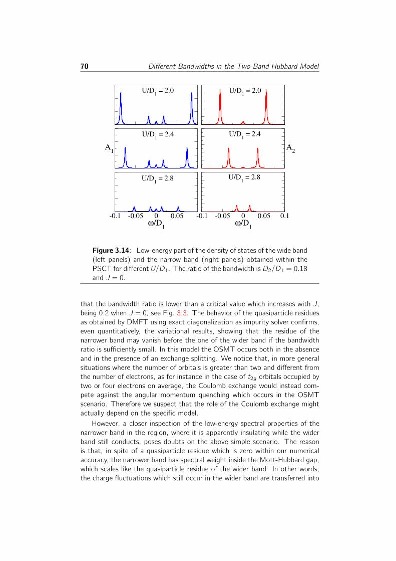
70 Different Bandwidths in the Two-Band Hubbard Model
A1 A2
-0.1 -0.05 0 0.05ω/D1
-0.1 -0.05 0 0.05 0.1ω/D1
U/D1 = 2.0 U/D1 = 2.0
U/D1 = 2.4
U/D1 = 2.8 U/D1 = 2.8
U/D1 = 2.4
Figure 3.14: Low-energy part of the density of states of the wide band
(left panels) and the narrow band (right panels) obtained within the
PSCT for different U/D1. The ratio of the bandwidth isD2/D1 = 0.18
and J = 0.
that the bandwidth ratio is lower than a critical value which increases with J,
being 0.2 when J = 0, see Fig. 3.3. The behavior of the quasiparticle residues
as obtained by DMFT using exact diagonalization as impurity solver confirms,
even quantitatively, the variational results, showing that the residue of the
narrower band may vanish before the one of the wider band if the bandwidth
ratio is sufficiently small. In this model the OSMT occurs both in the absence
and in the presence of an exchange splitting. We notice that, in more general
situations where the number of orbitals is greater than two and different from
the number of electrons, as for instance in the case of t2g orbitals occupied by
two or four electrons on average, the Coulomb exchange would instead com-
pete against the angular momentum quenching which occurs in the OSMT
scenario. Therefore we suspect that the role of the Coulomb exchange might
actually depend on the specific model.
However, a closer inspection of the low-energy spectral properties of the
narrower band in the region, where it is apparently insulating while the wider
band still conducts, poses doubts on the above simple scenario. The reason
is that, in spite of a quasiparticle residue which is zero within our numerical
accuracy, the narrower band has spectral weight inside the Mott-Hubbard gap,
which scales like the quasiparticle residue of the wider band. In other words,
the charge fluctuations which still occur in the wider band are transferred into

3.7 Discussion and Conclusions 71
the narrower one, as one can expect. This low-energy spectral weight is con-
centrated in two peaks symmetrically located around the chemical potential.
Roughly speaking, the distance of each peak from the chemical potential is 2J
plus a quantity of the order of the quasiparticle resonance width of the wider
band. Due to our limited numerical resolution, we can not establish rigorously
whether these two peaks (a) signal a narrow-gap semiconducting behavior, (b)
signal a semimetallic behavior, with a power-law vanishing density of states,
(c) or coexist with an extremely narrow resonance at the chemical potential,
with a spectral weight well below our numerical accuracy, just like the single
impurity does. Although the elements at our disposal do not definitely allow
to discriminate among these three scenarios, one can recognize that some of
them are more plausible than the others.
The first possibility (a) of a narrow-gap semiconductor seems very unlikely.
Indeed, in this case, the gap between the two low-energy peaks would open
large and then diminish as the quasiparticle resonance width of the wider band,
by further increasing the repulsion U. Therefore, the insulating character of
the narrower band would weaken by increasing U, which seems a bit unlikely.
Let us consider instead the scenario (b) of a semimetal. If taken literally,
it would imply a vanishingly small local magnetic susceptibility, while we ac-
tually find a very large one, much larger than the local susceptibility of the
wider band. However, a semimetallic behavior would imply, in our particle-hole
symmetric case, a breakdown of Fermi-liquid theory2. Therefore, a power-law
vanishing single-particle DOS might not necessarily conflict with almost free-
spin excitations in a scenario in which Fermi-liquid theory breaks down and
for instance spin-charge separation emerges. Although it might represent a
quite interesting circumstance, yet we could not find any physical arguments
justifying such a non-Fermi liquid behavior. Therefore, we are tempted to dis-
card it in favor of the more conservative scenario (c) in which the two peaks
coexist with a narrow resonance which remains tied at the chemical potential,
its spectral weight being smaller than our numerical accuracy. This resonance
should disappear right at the same U where the wider band ceases to conduct.
Finally, we note that, whatever the correct zero-temperature scenario, either
(b) or (c), there should exist a finite-temperature interval where the narrower
band loses its coherence unlike the wider one, which might display unusual
properties.
We terminate by mentioning that a parallel work by de’ Medici et al. [84]
studied the same problem using DMFT and a slave-spin mean-field approach
and reached similar conclusions. Moreover, in Ref. [18], the zero-temperature
properties of the self-energy of the wide band were investigated in detail and
2In the presence of particle-hole symmetry, the chemical potential is strictly zero whatever
is the interaction. On the other hand, if Fermi-liquid theory holds, then ImΣ(ω) ∼ ω2. In thiscase, it turns out that the value of the DOS at the chemical potential should not be affected
by U and J. Therefore, if one finds a different DOS from the bare one, that necessarily
implies a breakdown of Fermi-liquid theory.

72 Different Bandwidths in the Two-Band Hubbard Model
point in favor of scenario (b). Indeed, in their calculation, the low-energy
behavior of the self-energy displays non-Fermi liquid behavior. Finally, the
problem of the OSMT has continued to attract a lot of interest after the
completion of this work and an overview of the related activity can be found
in Ref. [65].

Chapter 4
Critical Behavior in ImpurityTrimers and Tetramers
We study two clusters of three and four Kondo impurities by means of Wilson’s
numerical renormalization group and conformal field theory. In both clusters,
the spin-1/2 magnetic moments are connected between them through a di-
rect exchange and each one is coupled to a conduction bath. The competition
between the Kondo effect, that is favored by a degenerate ground-state, and
the direct exchange, that tends to split this degeneracy, leads to rich phase
diagrams displaying stable phases separated by quantum critical lines. We pre-
cisely analyze these different phases by identifying the correct theory for every
fixed point of the renormalization group. We finally discuss their properties in
connection with the Mott transition as described by cluster dynamical mean-
field theory. Indeed, an impurity trimer and tetramer represent the simplest
clusters to simulate a Hubbard model on a triangular and square lattice. In
this context, we show that exotic behaviors that are found close to the Mott
transition in lattice models might well be traced back to instabilities, like an-
tiferromagnetism or Cooper pairing, that are already present at the impurity
level. The project presented in this chapter has been realized in collaboration
with M. Fabrizio, L. De Leo and P. Lecheminant.
4.1 Introduction
More than fifty years after its proposal [91], the Mott transition remains an
issue of current and broad interest, continually revived by the discovery of
strongly correlated materials which display anomalous phenomena in the vicin-
ity of a Mott insulating phase. The interaction-driven metal-to-insulator tran-
sition emerges out of the competition between the tendency of the electrons
to delocalize throughout the crystal, so as to maximize the band-energy gain,
and the Coulomb repulsion among the same electrons which, on the contrary,
tends to suppress valence fluctuations by localizing the carriers. Yet, as we
73

74 Critical Behavior in Impurity Trimers and Tetramers
have discussed in Chapter 1, realistic systems generally involve other energy
scales besides the Coulomb repulsion and the band-energy gain. Let us collec-
tively denote them by J. Approaching the Mott insulating phase, the entropy
is first reduced by the onset of a quasiparticle Fermi sea below a temperature
T ∗F , which gradually decreases because of strong correlations. At some point,
T ∗F will become of the same order as J and the new energy scales compete
with the formation of a degenerate quasiparticle gas. Indeed, the presence of
J provides new mechanisms to quench the entropy by freezing spin and or-
bital degrees of freedom, independently from the charge degrees of freedom.
This situation is actually realized in heavy fermion materials, where the Kondo
effect, favoring the formation of a coherent band of heavy quasiparticles, com-
petes with the RKKY interaction. Here, this competition is supposedly the key
to understand the anomalies which appear at the transition between the heavy
fermion paramagnet and the magnetically ordered phase [32, 106].
Competing Screening Mechanisms in Anderson Impurity Models
The heavy-fermion example is particularly pertinent for introducing the subject
of this chapter. Indeed, the competition between Kondo effect and RKKY
coupling has interesting consequences not only in the periodic Anderson model
but already at the level of Anderson impurity models. For instance, the phase
diagram of two spin-1/2 impurities coupled to a conduction bath but also
by a direct antiferromagnetic exchange has two limiting regimes: one where
each impurity is independently Kondo screened by the conduction electrons
and another where the direct exchange takes care of locking the impurity spins
into a singlet state, which is transparent to the conduction electrons. Under
particular circumstances, these two regimes are separated by a quantum critical
point, at which non-Fermi-liquid behavior emerges [5, 7, 60, 61, 62]. The
phase diagram grows richer when one considers three antiferromagnetically
coupled spin-1/2 impurities [55, 97]. In this case, besides a Kondo screened
regime, there are other phases where the direct exchange prevails even if it
is unable to fully quench the impurity degrees of freedom. This leads to
stable non-Fermi-liquid phases analogous to overscreened multi-channel Kondo
models [2, 3]. These clusters of impurity models are not only interesting
as simple attempts towards understanding the fully periodic Anderson model.
For instance, compact clusters of impurities are achievable experimentally by
adsorbing atoms on metallic surfaces. Indeed, trimers of Cr atoms have already
been realized on gold surfaces [58], which has actually motivated the most
recent theoretical activity on impurity trimers [55, 72, 75, 102]. In this context,
the major task is to identify those phases that are stable towards perturbations
which are generally allowed on metallic surfaces. Therefore, the quantum
critical points which separate stable phases are of minor interest, as they are
extremely unlikely to occur.

4.1 Introduction 75
Impurity Models and Dynamical Mean-Field Theory
The unstable critical points arise when the competition between Kondo screen-
ing and RKKY coupling is maximum. This is nothing but the impurity counter-
part of the situation when T ∗F ' J that we previously met in connection withthe Mott transition. This weak analogy turns into an actual equivalence within
the dynamical mean-field theory (DMFT) [42], which is the quantum analogue
of classical mean-field theory and, like the latter, becomes exact for infinite
coordination lattices (see Section 2.3). Within this limit, the single-particle
self-energy becomes fully local but maintains a non-trivial time-dependence.
In order to determine the frequency-dependent self-energy, within DMFT, one
solves an auxiliary single-impurity Anderson model, designed to have an impu-
rity self-energy that coincides with the local self-energy of the lattice model.
This requirement translates into an impurity model which is identified by the
same local interaction as the lattice model and by a coupling to a conduc-
tion bath which has to be self-consistently determined. As an approximation,
which is not exact in any limiting case, DMFT can be extended to include
short-range spatial components of the self-energy [69, 77, 81, 98, 105]. In
these novel versions, the lattice model is mapped onto a cluster of Anderson
impurities, subject to a self-consistency condition which is however no longer
uniquely determined by the requirement that the approximation becomes exact
in particular limits.
In the original single-site formulation of DMFT, the physics of the Anderson
impurity turned out to be a precious guideline to interpret the DMFT results.
This was possible mainly because a lot was already known about single-impurity
models. On the contrary, apart from few exceptions [60, 97], little is known
about impurity clusters. This is likely the reason why, in the cluster versions
of DMFT, not much attention has been paid so far to the impurity-cluster
models per se. In addition, since impurity clusters involve many energy scales,
including inter-impurity processes, it is not a priori evident whether there is
a common interpreting scheme like the Kondo physics in the single-impurity
case.
In order to clarify this issue, let us start by recalling some basic facts about
the single-site DMFT mapping onto impurity models. Within this mapping,
the quasiparticle effective Fermi temperature T ∗F translates into the Kondo
temperature TK of the impurity model. The self-consistency condition causes
TK to vanish at a finite value of U, which signals, in the lattice counterpart,
the onset of the Mott transition. This also implies that the metallic phase
just prior to the Mott transition translates into an Anderson impurity model
deep inside the Kondo regime, with a very narrow Kondo resonance and well
formed Hubbard side-bands [42]. The same behavior should remain even when
dealing with a cluster of impurities, which should translate into a cluster of
Kondo impurities that can effectively be regarded as a single impurity with
many internal degrees of freedom. The novelty stems from the other energy

76 Critical Behavior in Impurity Trimers and Tetramers
J
U/W
T = T
J
δ
T = TK FK F* *
Figure 4.1: Behavior versus U and the doping of the quasiparticle
Fermi temperature T ∗F , which translates within DMFT into the Kondo
temperature TK of the effective impurity model.
scales, which we denoted as J, that take care of quenching, in the Mott
insulator, the degrees of freedom other than the charge. Indeed, near the
Mott transition, J translates into additional processes, like for instance an
inter-impurity exchange, which tends to remove, completely or partially, the
degeneracy of the cluster. Consequently, J competes with the Kondo effect,
which takes better advantage the more degenerate the impurity cluster.
We note that this competition is always active in impurity clusters while
it is commonly absent in single-impurity models except in particular multi-
orbital cases [25, 26]. We believe that it is this additional ingredient, the
common denominator of all impurity-cluster models, which endows them with
the capability to provide a more faithful description of a realistic Mott transition
within DMFT.
Indeed, in the presence of J, the approach to the Mott transition displays,
as qualitatively shown in Fig. 4.1, a Kondo temperature smoothly decreasing
from its initial value W as U/W increases. Just before the transition, TKbecomes of order J. Analogously, (see Fig. 4.1) if one starts from the Mott
insulator and dopes it, TK will smoothly increase from its value TK = 0 at zero
doping, until it crosses a value of order J. This is the location of the, possibly
quantum critical, point which separates the Kondo screened phase, TK � J,
from the regime in which the internal screening mechanism prevails, J � TK .
Therefore, these critical points are always crossed in impurity models onto
which lattice models approaching a Mott transition are mapped within cluster
DMFT. The question is whether and how they may influence the behavior of
the lattice model after the DMFT self-consistency is carried out.
It has been argued [34, 36] that these impurity critical points do play an
important role in determining the phase diagram of the corresponding lattice
models. Indeed, near these unstable critical points, the impurity models dis-
play strongly enhanced local susceptibilities (or, equivalently, enhanced local

4.2 The Impurity Dimer 77
J KJ K
bath 1
J 21 bath 2
Figure 4.2: The impurity dimer with the Hamiltonian (4.1).
irreducible four-leg vertices) in several instability channels. Moreover, within
DMFT the irreducible four-leg vertices, which enter the Bethe-Salpeter equa-
tions, coincide with the local ones [42]. Therefore, it is reasonable to argue
that, after the full DMFT self-consistency is carried out, these local instabil-
ities may turn into full bulk instabilities, leading to symmetry broken phases
that partially hide what would have been the quantum critical regions around
the impurity unstable fixed points. This hypothesis, which has been tested
with success by a full DMFT calculation in a two-orbital Hubbard model [26],
suggests that the analysis of impurity-cluster models, even without any DMFT
self-consistency, may be very helpful in interpreting and even anticipating the
phase diagrams of strongly-correlated lattice models as uncovered by cluster
DMFT.
Following this speculation, we will, in this chapter, study the phase diagram
of the simplest Anderson impurity clusters, namely a trimer and a tetramer of
impurities, which can be used to implement a cluster DMFT calculation for
the Hubbard model on a square lattice. Needless to say, the interest in impu-
rity clusters goes beyond its possible relevance to Hubbard models on a square
lattice. As we previously mentioned, these clusters may be experimentally re-
alized on metallic surfaces or, eventually, by arranging quantum dots in proper
geometries. Moreover, as will emerge from our analysis, these models repre-
sent a theoretical challenge by themselves which requires the full machinery of
Wilson’s numerical renormalization group (NRG) and conformal field theory
(CFT) in order to have a detailed understanding (see Sections 2.6 and 2.7).
4.2 The Impurity Dimer
Before starting a systematic study of three and four impurity clusters, let us
briefly review the simplest example of an impurity dimer. This model was
originally studied by Jones and Varma [60, 61, 62] using NRG and the results
were later interpreted by Affleck and Ludwig [5, 7] within CFT. For simplicity,
we consider the impurity dimer drawn in Fig. 4.2 with the following Hamiltonian

78 Critical Behavior in Impurity Trimers and Tetramers
H =2∑a=1
[∑kσ
εk c†a kσca kσ +
JK2V
∑kk′αβ
Sa · c†a kα σαβ ca k′β
]
+ J S1 · S2 ≡2∑a=1
HKa + J S1 · S2,
(4.1)
which describes two spin-1/2 impurities, coupled together by an antiferro-
magnetic J, and both Kondo coupled to their own conduction bath by an
antiferromagnetic JK . The operators c†a kσ and ca kσ create and annihilate,
respectively, a conduction electron with spin σ and momentum k in the bath
a, and σ are the Pauli matrices. The two conduction baths are assumed to
be degenerate and particle-hole invariant. Furthermore, we assume that the
conduction-bath density of state is finite and smooth around the chemical po-
tential on a scale larger than the Kondo temperature. As a consequence, the
two baths, in the absence of the impurities, can be described [1] by a CFT
which includes independent spin SU(2)1 and charge isospin SU(2)1 symmetry
for each bath, namely an overall(SU(2)
(1)1 × SU(2)
(2)1
)charge
×(SU(2)
(1)1 × SU(2)
(2)1
)spin.
The subscript in SU(2)(a)k can be regarded here as the number of copies of
spin-1/2 electrons participating to the SU(2) algebra, while the superscript
refers to the bath.
The hypothesis behind the use of CFT is that, once the coupling to the
impurities is switched on, conformal invariance is not lost. The effect of the
impurities is then merely to change the conduction-bath boundary conditions
(BCs) among the conformally invariant ones. An important step in deter-
mining the allowed BCs is the conformal embedding [35], which amounts to
identifying the conformal field theories corresponding to the symmetry groups
under which the Hamiltonian of the bath plus the impurity remains invariant.
In the most favorable cases, the BCs that actually emerge correspond to con-
formally invariant BCs only within one of the different CFTs of the embedding.
The next useful information is that the conformally invariant BCs within each
sectors can be obtained by the so-called fusion hypothesis, according to which,
starting from the spectrum of a known BC, one can obtain all the others upon
fusion with the proper primary fields of the CFT (see Section 2.7).
In the model of Fig. 4.2, the isospin generators commute with the Hamil-
tonian even when JK and J are finite, and the charge sector can still be repre-
sented by two independent isospin SU(2)1. On the other hand, only the overall
spin SU(2) transformations leave the Hamiltonian invariant, which translates
into an SU(2)2 (two copies of electrons) CFT. As a result, the proper embed-
ding in the spin sector is [5]
SU(2)1 × SU(2)1 → SU(2)2 × Z2,

4.2 The Impurity Dimer 79
0 00Kondo screened Unscreened
J / J J / J* K K
Figure 4.3: Renormalization group flow diagram of the impurity
dimer.
where Z2 denotes an Ising CFT reflecting the symmetry under permutation of
the two baths.
The NRG phase diagram of the model [60, 61, 62] is sketched in Fig. 4.3
and includes, as we previously mentioned, two stable phases: a Kondo screened
and an unscreened phase, separated by an unstable critical point when J =
J∗ ' TK . Affleck and Ludwig [5, 7] realized that these different fixed points aredescribed by the three different BCs of the Ising CFT. The two stable phases
correspond to fixed BCs, where one Ising spin orientation is prohibited at the
boundary, and the unstable fixed point to a free BC, where both orientations
are allowed. Starting from the unscreened phase, the Kondo screened phase
is obtained by fusion with the Ising primary field ε of dimension 1/2, while the
unstable fixed point is obtained by fusion with the primary field σ of dimension
1/16.
As shown in Section 2.7, CFT also allows, by double-fusion, to deter-
mine the scaling dimensions of the relevant operators. It turns out that there
are three equally relevant (i.e. with dimension smaller than one) symmetry-
breaking perturbations which can destabilize the unstable fixed point. They
all have the same dimension 1/2 as the invariant operator which moves away
from the fixed point and corresponds to a deviation of J from its fixed point
value J∗ at fixed TK . The first perturbation is an opposite spin magnetization
for the two baths. The second is a BCS term in the inter-bath Cooper singlet
channel. The last perturbation corresponds to a direct hybridization between
the two baths breaking the independent conservation of charge.
The latter is very important. Indeed, let us suppose that, instead of two
spin-1/2 impurities, we have two single-orbital Anderson impurities with the
Hamiltonian
H =2∑a=1
[∑kσ
εk c†a kσca kσ −
tK√V
∑kσ
c†a kσda σ +H.c.
]− t⊥
∑σ
d†1σd2σ +H.c.+
U
2
2∑a=1
(na − 1)2,
(4.2)
where da σ are the annihilation operators for the impurity and na =∑σ d
†a σda σ.
It is actually the model (4.2) rather than (4.1) that has to be used to simulate,
80 Critical Behavior in Impurity Trimers and Tetramers
with a single dimer, a Hubbard model within cluster DMFT. As we previously
mentioned, the approach to the Mott transition corresponds to an impurity
model deep inside the Kondo regime, namely with U � tK , t⊥. Within this
limit, the model (4.2) can be mapped by a Schrieffer-Wolff transformation
onto (4.1), with J = 4t2⊥/U and JK = 4t2K/U. However, at next order in 1/U,
a local direct hybridization V among the baths is generated, with V ∼ JK t⊥/U.Although small, V is a relevant perturbation which makes the unstable fixed
point of the model (4.1) inaccessible in the model (4.2). Yet, since J � V ,
a quantum critical region, instead of a true quantum critical point, is still well
visible as was shown in Ref. [34]. In other words, the quantum phase transition
which occurs in model (4.1) turns into a very sharp crossover in (4.2). This
suggests that the unstable fixed point of the spin-dimer may still influence the
approach to the Mott transition in lattice models which map within DMFT
onto the impurity model (4.2). In particular, if the latter is used to mimic,
within cluster DMFT, a Hubbard model on a square lattice, we would spec-
ulate that near the Mott transition the inter-site singlet Cooper pairing and
the tendency to antiferromagnetic ordering are strongly enhanced, since both
are instability channels of the dimer fixed point (note that the hybridization
among the baths is explicitly present in the Hamiltonian). Most likely, antifer-
romagnetism prevails at half-filling, but upon doping, superconductivity might
still emerge [34].
4.3 The Impurity Trimer
Let us move now to our actual work and start considering the impurity trimer
drawn in Fig. 4.4 with the Hamiltonian
H =3∑a=1
HKa + J (S1 + S3) · S2 + J ′ S1 · S3, (4.3)
where HKa has been defined in (4.1). This model describes three spin-1/2 im-purities coupled together by antiferromagnetic J and J ′ and to their own con-
duction bath by JK > 0. As before, we assume that the baths are degenerate
and particle-hole invariant. When J ′ = 0 the trimer is the next simple cluster
beyond the dimer to represent a Hubbard model on a square lattice within clus-
ter DMFT. This would really be true only if we considered three single-orbital
Anderson impurities coupled by a single-particle hopping t⊥ rather than three
spin-1/2 moments coupled by an exchange J. However, in view of what we
discussed in the case of the dimer, the model (4.3) is more suitable to identify
unstable fixed points which might transform into sharp crossover regions in
the case of Anderson impurities because of the weak hybridization among the
baths generated by t⊥. For this reason, we will consider, both here for the
trimer and later for the tetramer, spin-1/2 Kondo impurities and treat the
hybridization among the baths as a perturbation.

4.3 The Impurity Trimer 81
bath 1
bath 2
bath 3
J K
J K
J K
1
2
3
J
J
J’
Figure 4.4: The impurity trimer with the Hamiltonian (4.3).
4.3.1 CFT Preliminaries for the Trimer
As in the dimer example, the trimer model (4.3) exhibits charge degrees of
freedom described by three independent isospin SU(2)(a)1 CFTs, a = 1, 2, 3.
The expression of the inter-impurity exchange naturally suggests how the spin
symmetry should be reduced. First, we have to couple the spin sectors of
baths 1 and 3 into an overall SU(2)2 via the embedding
SU(2)(1)1 × SU(2)
(3)1 → SU(2)
(1−3)2 × Z2,
where Z2 denotes the Ising CFT. Then, the SU(2)2 is coupled to the bath 2
into an overall SU(2)3 according to embedding
SU(2)(1−3)2 × SU(2)(2)1 → SU(2)3 × (TIM) ,
where TIM stands for the tricritical Ising model CFT. Combining everything
together, we see that the original symmetry of the three independent spin
SU(2)(a)1 is reduced to
SU(2)3 × Z2 × (TIM) .
This conformal embedding can be rigorously justified by the character decom-
position [35], namely by the formal identification of the free energies in the
original and in the decomposed theory (see Appendix A).

82 Critical Behavior in Impurity Trimers and Tetramers
× I ε t ε′′
σ σ′
I I ε t ε′′
σ σ′
ε ε I + t ε+ ε′′
t σ + σ′
σ
t t ε+ ε′′
I + t ε σ + σ′
σ
ε′′
ε′′
t ε I σ σ′
σ σ σ + σ′σ + σ
′σ I + ε+ t + ε
′′ε+ t
σ′
σ′
σ σ σ′
ε+ t I + ε′′
Table 4.1: Fusion rules of the tricritical Ising model.
The SU(2)k CFT has central charge c = 3k/(2+k). Its primary fields φ(k)2j
are labeled by a spin quantum number j = 0, . . . , k/2 and have the following
scaling dimensions and fusion rules:
∆(k)j = j(j + 1)/(2 + k)
j × j ′ = |j − j ′|+ (|j − j ′|+ 1) + · · ·+min(j + j ′, k − j − j ′).
The Ising CFT, with central charge c = 1/2, has three primary fields,
the identity I, the thermal energy εI and the order parameter σI [35]. Their
dimension and fusion rules [35, p. 221] are given by
∆I = 0, ∆εI = 1/2, ∆σI = 1/16
σI × σI = I + εI , σI × εI = σI , εI × εI = I.
Finally, the TIM has central charge c = 7/10 and six primary fields [35]:
the identity I, ε, t, ε′′, σ and σ
′. Their dimension are
∆I = 0, ∆ε = 1/10, ∆t = 3/5,
∆ε′′ = 3/2, ∆σ = 3/80, ∆σ′ = 7/16,
and the fusion rules [35, p. 224] between these fields are shown in Table 4.1.
As we previously mentioned, the possible conformally invariant boundary
conditions can be classified by means of the fusion hypothesis [2, 3, 7]. Starting
from the spectrum of a simple BC, for instance corresponding to JK = 0, one
can obtain the spectra of other allowed BCs upon fusion with the primary
fields of the CFTs. By comparing the low-energy spectra determined in this
way with those obtained by NRG, one can identify and characterize all fixed
points of the model.
4.3.2 Fixed Points in the Trimer Phase Diagram
In Fig. 4.5, we sketch the phase diagram of the impurity trimer as obtained
by NRG (see Section 2.6). The calculations were performed with Λ = 3.
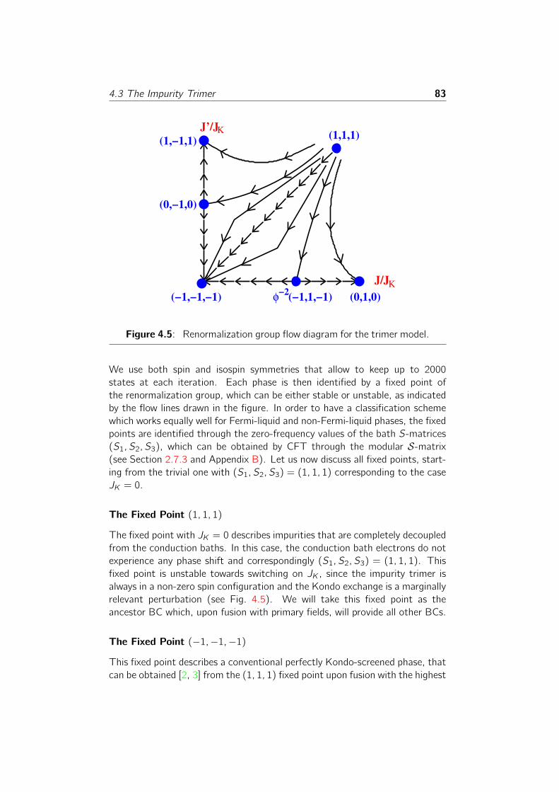
4.3 The Impurity Trimer 83
J’/J
J/J
(1,−1,1)
(0,−1,0)
φ−2(−1,−1,−1) (−1,1,−1) (0,1,0)
(1,1,1)K
K
Figure 4.5: Renormalization group flow diagram for the trimer model.
We use both spin and isospin symmetries that allow to keep up to 2000
states at each iteration. Each phase is then identified by a fixed point of
the renormalization group, which can be either stable or unstable, as indicated
by the flow lines drawn in the figure. In order to have a classification scheme
which works equally well for Fermi-liquid and non-Fermi-liquid phases, the fixed
points are identified through the zero-frequency values of the bath S-matrices
(S1, S2, S3), which can be obtained by CFT through the modular S-matrix(see Section 2.7.3 and Appendix B). Let us now discuss all fixed points, start-
ing from the trivial one with (S1, S2, S3) = (1, 1, 1) corresponding to the case
JK = 0.
The Fixed Point (1, 1, 1)
The fixed point with JK = 0 describes impurities that are completely decoupled
from the conduction baths. In this case, the conduction bath electrons do not
experience any phase shift and correspondingly (S1, S2, S3) = (1, 1, 1). This
fixed point is unstable towards switching on JK , since the impurity trimer is
always in a non-zero spin configuration and the Kondo exchange is a marginally
relevant perturbation (see Fig. 4.5). We will take this fixed point as the
ancestor BC which, upon fusion with primary fields, will provide all other BCs.
The Fixed Point (−1,−1,−1)
This fixed point describes a conventional perfectly Kondo-screened phase, that
can be obtained [2, 3] from the (1, 1, 1) fixed point upon fusion with the highest

84 Critical Behavior in Impurity Trimers and Tetramers
weight representation of the SU(2)3 CFT with j = 3/2. It is clear that this
phase extends in a whole region around the origin J = J ′ = 0 in Fig. 4.5.
Indeed, when J = J ′ = 0, each impurity is independently Kondo screened by
its own conduction bath and this perfect screening can not be affected by finite
J and J ′ much smaller than the Kondo temperature. It is far less obvious that
this fixed point remains stable for large J ' J ′. When J ′ = J � TK , the
impurity locks into two degenerate S=1/2 configurations. In the first, sites 1
and 3 are coupled into a triplet which in turn is coupled with site 2 into an
overall spin-1/2 configuration. Since this is even by interchanging 1 with 3,
we denote it as |e〉. The other configuration, which we denote as |o〉, is oddunder 1↔ 3 and corresponds to coupling sites 1 and 3 into a singlet, leavingbehind the free spin-1/2 moment of site 2. The Kondo exchange projected
onto this subspace reads
JK3|e〉〈e| S ·
(2J1(0)− J2(0) + 2J3(0)
)+ JK |o〉〈o| S · J2(0)
−JK√3
(|e〉〈o|+ |o〉〈e|
)S ·(J1(0)− J3(0)
),
(4.4)
where S describes the effective S=1/2 of the trimer, while Ja(0) is the spin
density of bath a = 1, 2, 3 at the impurity site, assumed to be the origin. All the
above screening channels flows to strong coupling within a one-loop calcula-
tion. Since it is readily shown that the impurity can be perfectly screened,
both in the spin and in the e-o channels, one has to conclude that the
whole line J = J ′ at finite JK corresponds to the Kondo screened fixed point
(−1,−1,−1), as shown in Fig. 4.5. A small deviation from J = J ′ splits
the degeneracy between |e〉 and |o〉 and would eventually destabilize this fixedpoint, the faster the smaller JK .
The Fixed Point (0, 1, 0)
This fixed point occurs for J � TK , J′ (see Fig. 4.5). The NRG spectrum is
shown at the far right of Fig. 4.6 and the energies are reported in Table 4.2.
This spectrum is compatible with that obtained by first fusing the (1, 1, 1)
fixed point with the j = 3/2 primary field of the SU(2)3 CFT and then with
the field σ′of the TIM. It is not difficult to realize that this fixed point is
equivalent to the non-Fermi-liquid phase of the S=1/2 two-channel Kondo
model [2, 3]. Indeed, if J ′ = 0 and J is very large, the trimer is locked into the
S=1/2 configuration which we previously denoted as |e〉, to indicate the evenparity upon 1 ↔ 3. According to (4.4), the Kondo exchange projected ontothis configuration is
S ·3∑a=1
J(a)K Ja(0) =
JK3S ·(2J1(0)− J2(0) + 2J3(0)
). (4.5)

4.3 The Impurity Trimer 85
-80 -40 0 40 800
0.2
0.4
0.6
0.8
1
Figure 4.6: Flow diagrams for J ′ = 0 and J slightly smaller (left) and
slightly larger (right) than the critical J∗. The intermediate, unstable
fixed point is clearly visible. The arrows mark the CFT predictions for
the location of the energy levels.
2I 2S Q Z2 TIM x − 3/16 ENRG
0 1 0 0 3/80 0 0.000000
1 0 1/4 1/16 0 1/8 0.126716
1 0 1/4 1/16 0 1/8 0.128870
1 2 1/4 0 3/80 1/2 0.498068
1 0 1/4 0 7/16 1/2 0.498105
0 1 1/2 0 3/80 1/2 0.499241
2 1 1/2 0 3/80 1/2 0.499241
0 1 0 1/2 3/80 1/2 0.500586
0 1 1/2 1/16 1/10 5/8 0.624506
2 1 1/2 1/16 1/10 5/8 0.624506
0 1 1/2 1/16 1/10 5/8 0.625623
2 1 1/2 1/16 1/10 5/8 0.625623
1 2 1/4 1/16 1/10 5/8 0.628025
1 2 1/4 1/16 1/10 5/8 0.628167
Table 4.2: Lowest energy states as obtained by CFT and NRG for
the fixed point (S1, S2, S3) = (0, 1, 0). The states are given with their
total isospin I and spin S. The columns Q, Z2 and TIM indicate the
contributions from the charge, the Ising and the TIM CFT respectively.

86 Critical Behavior in Impurity Trimers and Tetramers
Hence, while bath 1 and 3 are still antiferromagnetically coupled, the cou-
pling with bath 2 turns effectively ferromagnetic. The ordinary one-loop
renormalization group calculation would predict that the Kondo exchanges
J(1)K = J
(3)K > 0 flow towards strong coupling, while J
(2)K < 0 flows towards
zero. This suggests that a model with J(1)K = J
(3)K � −J
(2)K > 0 should behave
asymptotically as (4.5). If J(2)K = 0 this is just the two-channel spin-1/2 impu-
rity model [2, 3, 6], which is non Fermi-liquid with S-matrices S1 = S3 = 0. It
is easy to realize that the small ferromagnetic J(2)K transforms into an antifer-
romagnetic exchange with the spin-density operators of baths 1 and 3, which
is irrelevant. Indeed, the operator (J1+J2+J3) ·(J1−2J2+J3) has dimension3/2. Consequently, we expect that this phase should be non-Fermi-liquid and
identified by the S-matrices (S1, S2, S3) = (0, 1, 0), as is indeed confirmed by
CFT. In addition, through the modular S-matrix (see Section 2.7.2 and Ap-pendix B), one can show that the zero-temperature entropy S(0) = 1/2 ln 2 is
finite and coincides with that of the S=1/2 two-channel Kondo model. Since
σ′ × σ′ = I + ε′′ and the dimension of ε′′ is 3/2 > 1, this fixed point is stableto symmetry-preserving perturbations. However, there are several symmetry-
breaking relevant perturbations of dimension 1/2. One of them corresponds
to the staggered magnetization
J1 − 2J2 + J3. (4.6)
All the other relevant operators break the degeneracy between bath 1 and 3
as well. This is for instance the case for the spin-singlet operator
J2 ·(J1 − J3
), (4.7)
which is indeed known to be a relevant perturbation at the overscreened non-
Fermi-liquid fixed point [8]. This phase extends at finite J ′ because a small J ′
does not generate any symmetry-breaking relevant perturbation.
The approach to the fixed point is controlled by two leading irrelevant
operators of dimension 3/2: ε′′and the scalar product of the staggered mag-
netization (4.6) with the first spin descendant. Similarly to the overscreened
two-channel Kondo model [2, 3], these operators produce logarithmic singu-
larities in the impurity contribution to the specific heat coefficient and to the
magnetic susceptibility, Cimp/T ∼ χimp ∼ ln(1/T ).
The Fixed Point φ−2 (−1, 1,−1)
Since the Kondo screened phase (−1,−1,−1) and the non-Fermi liquid phase(0, 1, 0) are essentially different, an unstable critical line separates them (see
Fig. 4.5). The NRG spectrum for this line is shown in the central part of
Fig. 4.6 and the corresponding energy levels are reported in Table 4.3. We
find that the NRG spectrum can be reproduced by fusing the (1, 1, 1) fixed
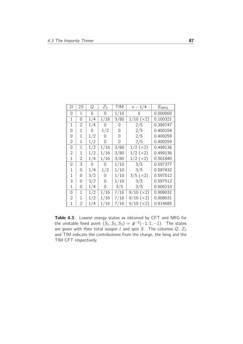
4.3 The Impurity Trimer 87
2I 2S Q Z2 TIM x − 1/4 ENRG
0 1 0 0 1/10 0 0.000000
1 0 1/4 1/16 3/80 1/10 (×2) 0.100321
1 2 1/4 0 0 2/5 0.396747
0 1 0 1/2 0 2/5 0.400154
0 1 1/2 0 0 2/5 0.400259
2 1 1/2 0 0 2/5 0.400259
0 1 1/2 1/16 3/80 1/2 (×2) 0.499136
2 1 1/2 1/16 3/80 1/2 (×2) 0.499136
1 2 1/4 1/16 3/80 1/2 (×2) 0.501840
0 3 0 0 1/10 3/5 0.597377
1 0 1/4 1/2 1/10 3/5 0.597432
1 0 3/2 0 1/10 3/5 (×2) 0.597512
3 0 3/2 0 1/10 3/5 0.597512
1 0 1/4 0 3/5 3/5 0.606210
0 1 1/2 1/16 7/16 9/10 (×2) 0.908031
2 1 1/2 1/16 7/16 9/10 (×2) 0.908031
1 2 1/4 1/16 7/16 9/10 (×2) 0.914685
Table 4.3: Lowest energy states as obtained by CFT and NRG for
the unstable fixed point (S1, S2, S3) = φ−2(−1, 1,−1). The statesare given with their total isospin I and spin S. The columns Q, Z2and TIM indicate the contributions from the charge, the Ising and the
TIM CFT respectively.

88 Critical Behavior in Impurity Trimers and Tetramers
-80 -40 0 40 800
0.2
0.4
0.6
0.8
1
Figure 4.7: Flow diagrams for J = 0.01 and J ′ slightly smaller (left)
and slightly larger (right) than the critical J ′∗. The intermediate, unsta-
ble fixed point is clearly visible. The arrows mark the CFT predictions
for the location of the energy levels.
point with the j = 3/2 primary field of the SU(2)3 CFT and with the field
ε of the TIM. The S-matrices are φ−2 (−1, 1,−1) and the residual entropyis S(0) = lnφ, where φ = (1 +
√5)/2 is the golden ratio. Since ε × ε =
I + t, the operator which moves away from the critical line has dimension
3/5. In other words, a small deviation δ from the line introduces a cross-over
energy scale δ5/2. The most relevant symmetry-breaking operator is still the
staggered magnetization (4.6), which now has dimension 2/5. Once more, the
approach to this fixed point is controlled by the scalar product of the staggered
magnetization with the first Kac-Moody descendant of the SU(2)3 CFT, which
has dimension 1 + 2/5. Analogously to the multichannel Kondo [2, 3], this
operator produces impurity contributions to the specific-heat coefficient and
magnetic susceptibility that diverge like T−1/5.
The spin-singlet operator (4.7) is also relevant, although with a smaller
dimension 3/5. In addition, there is a new class of dimension-3/5 operators
which correspond to coupling into a spin-singlet two particles, or one hole and
one particle, belonging to bath 2 and either bath 1 or 3. This implies two
important features: (i) This fixed point, like the dimer one, is destabilized
by a single-particle hybridization between the baths, hence it would never be
reachable in a model of coupled Anderson impurities, as we expected; (ii) The
inter-bath Cooper pairing instability is again enhanced, like in the dimer model.

4.3 The Impurity Trimer 89
2I 2S Q Z2 TIM x − 5/16 ENRG
1 0 1/4 1/16 0 0 0.00000
0 1 0 1/16 1/10 0 0.00001
0 1 1/2 0 3/80 3/8 (×2) 0.37234
2 1 1/2 0 3/80 3/8 (×2) 0.37234
1 0 1/4 0 7/16 3/8 (×2) 0.37245
1 2 1/4 0 3/80 3/8 (×2) 0.37245
0 1 0 1/16 3/5 1/2 0.49748
0 3 0 1/16 0 1/2 0.49748
1 2 1/4 1/16 1/10 1/2 0.49765
0 1 1/2 1/16 1/10 1/2 0.49797
2 1 1/2 1/16 1/10 1/2 0.49797
1 0 3/4 1/16 0 1/2 (×2) 0.49813
3 0 3/4 1/16 0 1/2 0.49813
0 1 1/2 1/2 3/80 7/8 (×2) 0.88039
2 1 1/2 1/2 3/80 7/8 (×2) 0.88039
1 0 1/4 1/2 7/16 7/8 (×2) 0.88048
1 2 1/4 1/2 3/80 7/8 (×2) 0.88048
Table 4.4: Lowest energy states as obtained by CFT and NRG for the
fixed point (S1, S2, S3) = (0,−1, 0). The states are given with theirtotal isospin I and spin S. The columns Q, Z2 and TIM indicate the
contributions from the charge, the Ising and the TIM CFT respectively.
The Fixed Points (1,−1, 1) and (0,−1, 0)
These two fixed points occur when J ′ > J is larger or comparable to the Kondo
temperature. They have a simple explanation. Indeed, when J = 0, site 2 is
only coupled to bath 2 with a Kondo exchange, leading to a full screening,
i.e. S2 = −1. Sites 1 and 3 plus their own baths realize once more a two-impurity Kondo model which, as discussed before, has two stable regimes. One
regime, for J ′ � TK , is Kondo screened and has S1 = S3 = −1 so that it isdescribed by the fixed point (S1, S2, S3) = (−1,−1,−1) (see Fig. 4.5). Theother regime, J ′ � TK , has (S1, S2, S3) = (1,−1, 1) in Fig. 4.5. These tworegimes are clearly stable towards switching on a small J � J ′. When J = 0,
we also know that an unstable fixed point at J ′ = J ′∗ ∼ TK separates these
two stable phases and is identified by S1 = S3 = 0, hence the label (0,−1, 0)in Fig. 4.5. Since site 2 is tightly bound into a singlet state with bath 2,
a finite but small J � TK will simply generate a ferromagnetic exchange of
order −J2/TK by virtually exciting the singlet state. The net effect is that theunstable fixed point at J = 0 is just the endpoint of another critical line which,
for J � TK , moves to larger values of J′. This has been checked by the NRG

90 Critical Behavior in Impurity Trimers and Tetramers
calculations, and we show the flow diagram around this line in Fig. 4.7. From
the CFT viewpoint, the (1,−1, 1) or (0,−1, 0) fixed points can be obtainedby fusing with the j = 3/2 primary field of the SU(2)3 and with ε
′′of the TIM
or σI of the Ising CFT, respectively. For comparison, we report the energies
obtained by NRG at the fixed point (0,−1, 0) in Table 4.4. The properties ofthe unstable (0,−1, 0) critical line are the same as those of the dimer criticalpoint. In particular, there is a relevant operator in the singlet Cooper channel
that now involves pairing among baths 1 and 3, as well as an equally relevant
operator which corresponds to an opposite magnetization of bath 1 and 3, i.e.
J1 − J3.
4.3.3 Concluding Remarks About the Trimer
We have shown that the trimer model (4.3) has quite a rich phase diagram,
drawn in Fig. 4.5. Besides the three different stable phases, we have found
two unstable critical lines with some notable features:
(1) Both critical lines turn into crossover regions, which we believe should
be sharp, if instead of three coupled spin-1/2 Kondo impurities we had
considered three Anderson impurities, with an on-site Hubbard U, cou-
pled by a hopping t between sites 2 and 1 and 2 and 3, and a hopping
t ′ between sites 1 and 3.
(2) Both lines are unstable towards a magnetic symmetry breaking deter-
mined by the largest among J and J ′, namely J1 − 2J2 + J3 for J > J ′
and J1 − J3 for J ′ > J.
(3) Both lines are also unstable in a singlet Cooper channel. In particular,
for J > J ′ along the critical line φ−2 (−1, 1,−1), the instability channelcorresponds to an inter-site pairing along bonds 1-2 and 2-3. On the
contrary, along the line (0,−1, 0) for J ′ > J, it is the inter-site pairing
along bond 1-3 which is singular.
The Trimer with C3 Symmetry and the Hubbard Model on a Triangular
Lattice
Let us conclude by noting that, for J = J ′, the trimer is actually the simplest
cluster to simulate, within DMFT, a Hubbard model on a triangular lattice.
Yet, as we mentioned several times, the trimer representative of a Hubbard
model very close to a Mott transition, necessarily includes, besides the inter-
impurity exchange J = J ′, a weak inter-bath hybridization, generally invariant
only under global U(1) gauge-symmetry, SU(2) spin-rotations as well as under
C3 symmetry.
A trimer coupled to three baths with C3 symmetry was studied by NRG
by Paul and Ingersent [97], who found a phase diagram which contains three

4.4 The Impurity Tetramer 91
stable phases: the perfectly Kondo screened phase, our (−1,−1,−1) fixedpoint, and two non-Fermi-liquid regimes, which they denoted as Isospin-Kondo
and Frustrated-Kondo. In other words, the (−1,−1,−1) fixed point at J = J ′is destabilized by an hybridization among the baths that preserves the C3symmetry, provided it is large compared with the Kondo temperature. Trans-
lated within DMFT language, this should imply that the instability of the
(−1,−1,−1) fixed point is very likely to be encountered by the trimer, repre-sentative of a Hubbard model on a triangular lattice, on the way to the Mott
insulating phase, TK → 0. Which of the two non-Fermi-liquid regimes mayoccur depends on the density of states at the Fermi energy projected onto the
three helicity states, h = 0,±1, of the cluster
ρh =1
V
∑k
δ (εk − εF )∣∣∣1 + eih2π/3 eik·a + e−ih2π/3 eik·b∣∣∣2 ,
where εk is the band energy of the triangular lattice, while a = (1, 0) and
b = (1/2,√3/2) are the unit lattice vectors. For the standard Hubbard model
with real nearest-neighbor hopping, ρ±1 > ρ0. This suggests that the non-
Fermi-liquid phase pertinent to this case is likely the Isospin-Kondo regime.
The Frustrated-Kondo regime, which requires ρ0 > ρ±1, might occur for in-
stance on a triangular lattice with purely imaginary nearest-neighbor hopping.
Incidentally, this is quite a peculiar model in which, although parity and time
reversal are broken, but not their product, particle-hole symmetry is preserved.
In both cases, the approach to the Mott transition should be influenced
by the critical point which separates the Fermi-liquid phase from the non-
Fermi-liquid one. However, the conformal embedding we have adopted so far
is no longer appropriate to describe both these critical points as well as the
Isospin-Kondo and the Frustrated-Kondo regimes, since it assumes indepen-
dent charge conservation in each bath. The correct embedding has recently
been found by Ingersent et al. [55], although it has been used only to discuss
the Isospin- and Frustrated-Kondo regimes and not the two unstable fixed
points, which would be of interest in connection with cluster DMFT.
4.4 The Impurity Tetramer
The other cluster that we consider is an impurity tetramer, as drawn in
Fig. 4.8. The properties of this cluster are still under current investigation
and we present hereunder the preliminary results that we have obtained. The
Hamiltonian is given by
H =4∑a=1
HKa + J (S1 + S3) · (S2 + S4) + J ′ (S1 · S3 + S2 · S4) . (4.8)
This model describes four spin-1/2 impurities, coupled together by a nearest
J, and next-nearest neighbor J ′, antiferromagnetic exchanges. In addition,

92 Critical Behavior in Impurity Trimers and Tetramers
bath 2
bath
1bath 3
J K
J KJ K
J K
bath 4
J’
J J
JJ
J’31
2
4x
y
Figure 4.8: The impurity tetramer with the Hamiltonian 4.8.
each spin is Kondo coupled to its conduction bath by JK > 0. The four baths
are degenerate and particle-hole invariant. Clearly, the tetramer can be used
to represent the Hubbard model on a square lattice within the framework of
cluster DMFT. Again, one should in principle consider Anderson impurities,
but in order to facilitate the identification of fixed points, we prefer to use
Kondo impurities and discuss the effect of the hybridization between the baths
by treating it as a perturbation.
4.4.1 CFT Preliminaries for the Tetramer
As usual, given our choice of the model (4.8), the charge degrees of freedom
can be described by four independent SU(2)1 CFTs, one for each bath. For
the spin symmetry, the way the impurities are coupled by the direct exchange
naturally leads to the following conformal embedding scheme: First, we couple
the spin sectors of baths 1 and 3 into an overall SU(2)2 × Z2 as in the caseof the impurity trimer. The same procedure is applied to the baths 2 and 4
and we get (SU(2)
(1)1 × SU(2)
(3)1
)×(SU(2)
(2)1 × SU(2)
(4)1
)→(SU(2)
(1−3)2 × Z(1)2
)×(SU(2)
(2−4)2 × Z(2)2
).

4.4 The Impurity Tetramer 93
Field Dimension
I 0 x2 + y2
θ 1 xy(x2 − y2)φ3/2 3/2 x(x2 − y2); y(x2 − y2)φ1/24 1/24
φ1/6 1/6 x ; y
φ3/8 3/8
φ2/3 2/3 x2 − y2; xyφ25/24 25/24
σ(i=1,2) 1/16
τ (i=1,2) 9/16
Table 4.5: Primary fields of the c = 1 CFT with their dimensions.
Some fields transform according to irreducible representations of C4vand the corresponding functions of coordinates are shown in the last
column.
The two SU(2)2 are then coupled together into an SU(2)4 and leave behind
a CFT with central charge c = 1. The resulting embedding is
SU(2)4 × Z(1)2 × Z(2)2 ×
[c = 1 (CFT)
],
where c = 1 CFT stands for the Z2 orbifold of a free bosonic CFT [9, 35]
with compactification radius R =√12. This embedding can again be proven
rigorously through the character decomposition, as shown in Appendix A.
The c = 1 CFT contains 13 primary fields, some of them being twice
degenerate. We list them with their dimension in Table 4.5. Some of the
primary fields transform like irreducible representations of the C4v symmetry
group and we indicate, in Table 4.5, the functions of coordinates that transform
in the same way. The fusion rules between the primary fields can be found in
Ref. [35, p. 784].
4.4.2 Fixed Points in the Tetramer Phase Diagram
In Fig. 4.9, we sketch the phase diagram of (4.8) as obtained by NRG. The
calculations were performed with Λ = 10. We use the spin symmetry and the
conservation of charge in all four channels. At every NRG iteration, ∼ 2000states are kept. As before, each fixed point of the renormalization group
is identified by the S-matrices (S1, S2, S3, S4)(n), where the superscript (n)
is introduced to distinguish between different fixed points with the same S-
matrices. Let us describe the different fixed points that we find.
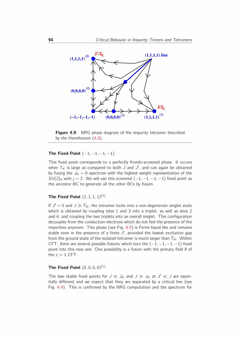
94 Critical Behavior in Impurity Trimers and Tetramers
(0,0,0,0) (1,1,1,1)
J/J
(0,0,0,0)
(1,1,1,1)J’/J
(1) (1)
(2)
(2) (1,1,1,1) line
(−1,−1,−1,−1)
K
K
Figure 4.9: NRG phase diagram of the impurity tetramer described
by the Hamiltonian (4.8).
The Fixed Point (−1,−1,−1,−1)
This fixed point corresponds to a perfectly Kondo-screened phase. It occurs
when TK is large as compared to both J and J′, and can again be obtained
by fusing the JK = 0 spectrum with the highest weight representation of the
SU(2)4 with j = 2. We will use this screened (−1,−1,−1,−1) fixed point asthe ancestor BC to generate all the other BCs by fusion.
The Fixed Point (1, 1, 1, 1)(1)
If J ′ = 0 and J � TK , the tetramer locks into a non-degenerate singlet state
which is obtained by coupling sites 1 and 3 into a triplet, as well as sites 2
and 4, and coupling the two triplets into an overall singlet. This configuration
decouples from the conduction electrons which do not feel the presence of the
impurities anymore. This phase (see Fig. 4.9) is Fermi-liquid like and remains
stable even in the presence of a finite J ′, provided the lowest excitation gap
from the ground state of the isolated tetramer is much larger than TK . Within
CFT, there are several possible fusions which turn the (−1,−1,−1,−1) fixedpoint into this new one. One possibility is a fusion with the primary field θ of
the c = 1 CFT.
The Fixed Point (0, 0, 0, 0)(1)
The two stable fixed points for J � JK and J � JK at J′ � J are essen-
tially different and we expect that they are separated by a critical line (see
Fig. 4.9). This is confirmed by the NRG computation and the spectrum for

4.4 The Impurity Tetramer 95
2I 2S Q Z(1)2 Z
(2)2 c = 1 x − 1/6 ENRG
0 0 0 0 0 1/6 0 0.00000
0 2 0 0 0 1/6 1/3 0.33123
1 1 1/4 1/16 0 1/16 1/3 (×2) 0.33898
1 1 1/4 0 1/16 1/16 1/3 (×2) 0.33898
0 0 1/2 1/16 1/16 1/24 1/2 (×4) 0.49602
2 0 1/2 1/16 1/16 1/24 1/2 (×4) 0.49602
0 2 0 1/2 0 0 2/3 0.67050
0 2 0 0 1/2 0 2/3 0.67050
0 2 1/2 0 0 0 2/3 (×2) 0.67050
2 2 1/2 0 0 0 2/3 (×2) 0.67050
1 1 1/4 1/16 0 9/16 5/6 (×2) 0.81649
1 1 1/4 0 1/16 9/16 5/6 (×2) 0.81649
1 1 3/4 0 1/16 1/16 5/6 (×4) 0.81649
3 1 3/4 0 1/16 1/16 5/6 (×2) 0.81649
1 1 3/4 1/16 0 1/16 5/6 (×4) 0.81649
3 1 3/4 1/16 0 1/16 5/6 (×2) 0.81649
1 3 1/4 1/16 0 1/16 5/6 (×2) 0.82156
1 3 1/4 0 1/16 1/16 5/6 (×2) 0.82156
0 2 1/2 1/16 1/16 1/24 5/6 (×4) 0.84007
2 2 1/2 1/16 1/16 1/24 5/6 (×4) 0.84007
1 1 1/4 1/16 1/2 1/16 5/6 (×2) 1.01981
1 1 1/4 1/2 1/16 1/16 5/6 (×2) 1.01981
Table 4.6: Lowest energy states as obtained by CFT and NRG for
the unstable fixed point (S1, S2, S3, S4) = (0, 0, 0, 0)(1). The states
are given with their total isospin I and spin S. The columns Q, Z(a)2
and c = 1 indicate the contributions from the charge, the Ising and
the c = 1 CFT respectively.
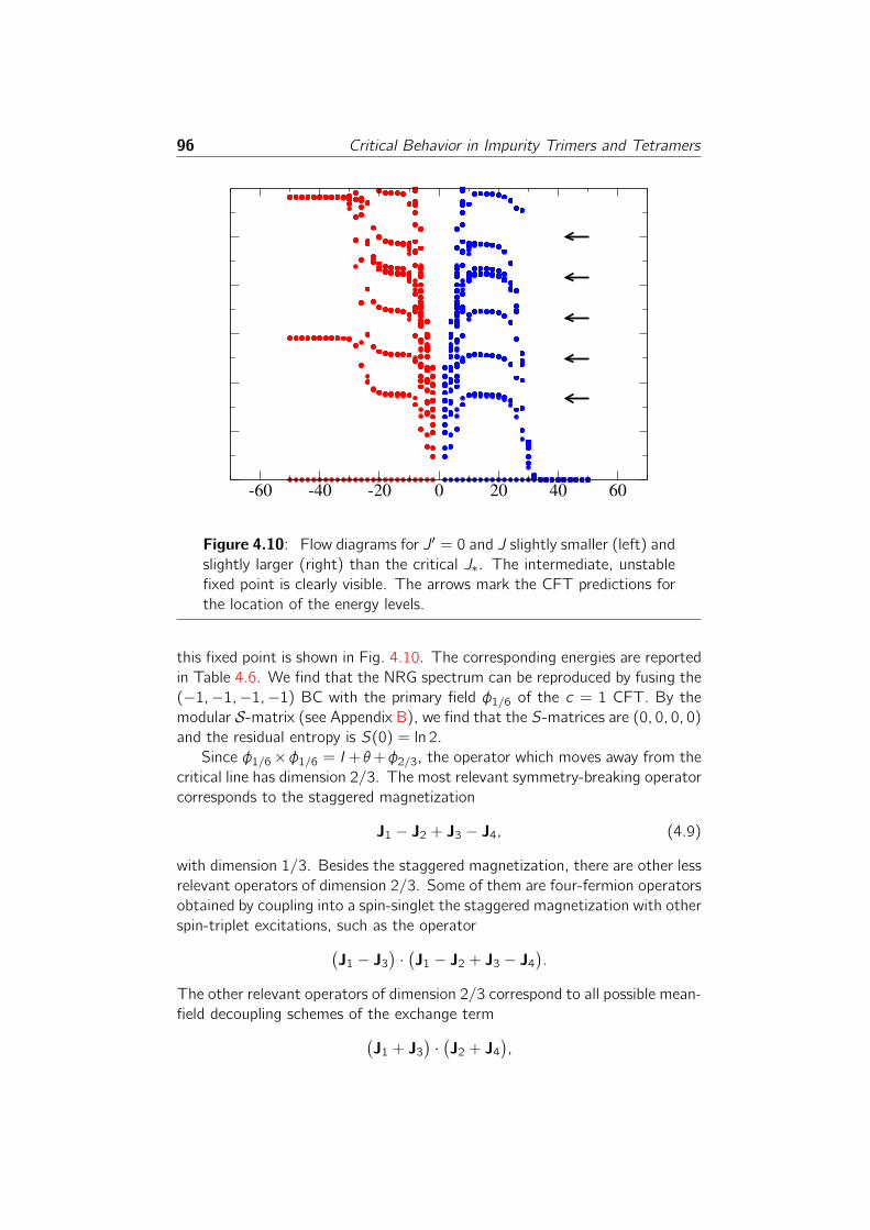
96 Critical Behavior in Impurity Trimers and Tetramers
-60 -40 -20 0 20 40 60
Figure 4.10: Flow diagrams for J ′ = 0 and J slightly smaller (left) and
slightly larger (right) than the critical J∗. The intermediate, unstable
fixed point is clearly visible. The arrows mark the CFT predictions for
the location of the energy levels.
this fixed point is shown in Fig. 4.10. The corresponding energies are reported
in Table 4.6. We find that the NRG spectrum can be reproduced by fusing the
(−1,−1,−1,−1) BC with the primary field φ1/6 of the c = 1 CFT. By themodular S-matrix (see Appendix B), we find that the S-matrices are (0, 0, 0, 0)and the residual entropy is S(0) = ln 2.
Since φ1/6×φ1/6 = I+ θ+φ2/3, the operator which moves away from thecritical line has dimension 2/3. The most relevant symmetry-breaking operator
corresponds to the staggered magnetization
J1 − J2 + J3 − J4, (4.9)
with dimension 1/3. Besides the staggered magnetization, there are other less
relevant operators of dimension 2/3. Some of them are four-fermion operators
obtained by coupling into a spin-singlet the staggered magnetization with other
spin-triplet excitations, such as the operator(J1 − J3
)·(J1 − J2 + J3 − J4
).
The other relevant operators of dimension 2/3 correspond to all possible mean-
field decoupling schemes of the exchange term(J1 + J3
)·(J2 + J4
),

4.4 The Impurity Tetramer 97
2I 2S Q Z(1)2 Z
(2)2 c = 1 x − 1/8 ENRG
0 0 0 1/16 1/16 0 0 0.00000
1 1 1/4 1/16 0 1/16 3/8 (×2) 0.37800
1 1 1/4 0 1/16 1/16 3/8 (×2) 0.37800
0 2 0 1/16 1/16 1/6 1/2 (×2) 0.46976
0 0 1/2 1/16 1/16 0 1/2 (×2) 0.47207
2 0 1/2 1/16 1/16 0 1/2 (×2) 0.47207
0 0 1/2 0 0 3/8 3/4 (×4) 0.78136
2 0 1/2 0 0 3/8 3/4 (×4) 0.78136
0 2 1/2 0 0 1/24 3/4 (×4) 0.78137
2 2 1/2 0 0 1/24 3/4 (×4) 0.78137
1 1 1/4 0 1/16 9/16 7/8 (×2) 0.88754
1 1 1/4 1/16 0 9/16 7/8 (×2) 0.88754
1 3 1/4 0 1/16 1/16 7/8 (×2) 0.88755
1 3 1/4 1/16 0 1/16 7/8 (×2) 0.88755
1 1 3/4 0 1/16 1/16 7/8 (×4) 0.89000
3 1 3/4 0 1/16 1/16 7/8 (×2) 0.89000
1 1 3/4 1/16 0 1/16 7/8 (×4) 0.89000
3 1 3/4 1/16 0 1/16 7/8 (×2) 0.89000
1 1 1/4 1/16 1/2 1/16 7/8 (×2) 1.09484
1 1 1/4 1/2 1/16 1/16 7/8 (×2) 1.09484
Table 4.7: Lowest energy states as obtained by CFT and NRG for
the unstable fixed point (S1, S2, S3, S4) = (0, 0, 0, 0)(2). The states
are given with their total isospin I and spin S. The columns Q, Z(a)2
and c = 1 indicate the contributions from the charge, the Ising and
the c = 1 CFT respectively.
into inter-bath bilinear operators. Among them, we just mention the inter-bath
hopping ∑σ
(c†1σ + c
†3σ
)(c2σ + c4σ
)+H.c.,
as well as the d-wave Cooper pairing1
(c†1↑ − c
†3↑)(c†2↓ − c
†4↓)−(↑↔↓
).
1In the reference frame of Fig. 4.8 this corresponds to a Cooper pair of dxy symmetry.
However, in the reference frame conventionally used for square lattices, which is rotated by
90 degrees, it corresponds to dx2−y2 .

98 Critical Behavior in Impurity Trimers and Tetramers
The Fixed Points (1, 1, 1, 1)(2) and (0, 0, 0, 0)(2)
If J = 0, sites 1 and 3 are decoupled from sites 2 and 4, hence the tetramer
reduces to two independent Kondo dimers. If J ′ � TK each pair of impurities,
1 and 3 or 2 and 4, is strongly bound into a singlet which decouples from
the conduction electrons. This fixed point is clearly stable to switching on
a small J. Hence, in analogy with the dimer, one should obtain it from the
(−1,−1,−1,−1) fixed point upon fusion with ε(1)I ε(2)I , where ε
(a)I , a = 1, 2,
are the energy operators of the two Ising CFTs. The NRG spectrum agrees
with this prediction, not only for small J, but for the whole region J ′ > J with
J ′ � TK , see Fig. 4.9. Once again, this unscreened regime is separated from
the Kondo regime by a critical line which is the same as in the impurity dimer.
It is therefore obtained [5] from the (−1,−1,−1,−1) fixed point upon fusionwith σ
(1)I σ
(2)I and it is identified by zero scattering matrices (0, 0, 0, 0)
(2) (see
Fig. 4.9), and by a residual entropy S(0) = ln 2. The energies obtained by
NRG for this fixed point are shown in Table 4.7 and agree well with the CFT
prediction. Besides the dimension-1/2 operator which moves away from this
critical point, there are several symmetry-breaking perturbations with the same
dimension: the direct hybridization among baths 1 and 3, as well as among 2
and 4; the spin magnetization J1− J3 and J2− J4; the 1-3 and 2-4 inter-bathsinglet Cooper pairing.
The (1, 1, 1, 1) Line
If J = J ′ � TK , the tetramer locks into a doubly degenerate spin-singlet state.
One state in the doublet is the singlet formed by two triplets, one between
sites 1 and 3, the other between sites 2 and 4. In our reference frame, (see
Fig. 4.8) this state has x2−y2 symmetry. The second state is instead the prod-uct of two singlets, between sites 1 and 3 and between 2 and 4. It transforms
like the product x y . The Kondo exchange provides a coupling between these
two configurations only at second order in JK , which is an irrelevant quartic
conduction-electron operator. Therefore, the tetramer decouples asymptoti-
cally from the conduction baths, and its degeneracy remains unchanged. This
is confirmed by the NRG calculation, which shows the same Fermi-liquid spec-
trum as in the absence of the impurity-cluster except that every state is doubly
degenerate. This phase is the analogous of a first-order line, hence the label
“(1, 1, 1, 1) line” in Fig. 4.8, and the splitting of the double degeneracy of the
tetramer is described by a relevant operator of dimension 0.
The Intermediate Fixed Point
The NRG calculations show that the two critical lines corresponding to the
fixed points (0, 0, 0, 0)(1,2) merge together at an unstable fixed point which
is the ending point of the (1, 1, 1, 1) line. This fixed point is unstable in all

4.5 Conclusions 99
directions and it has so far been impossible to find compatible BCs and low-
energy spectrum. A more precise identification of this fixed point is under
current investigation.
4.5 Conclusions
In this chapter, we have studied two clusters of impurities by means of Wilson’s
numerical renormalization group and conformal field theory. Even if the two
clusters are different, the phase diagrams of the impurity trimer and tetramer
share striking similarities. In both cases, stable phases are separated by critical
lines that show non-Fermi liquid behavior. The unstable fixed points emerge
from the competition between the Kondo effect that gains energy if the ground
state is degenerate and the RKKY interaction that splits this degeneracy. As
a result, these fixed points have many instabilities, but magnetism always
appears as being the most relevant one. Actually, going from the trimer to
the tetramer, the magnetic instability becomes even more relevant. Besides
magnetization, Cooper-pair instabilities are also present.
Let us discuss what might be the effects of these instabilities if these
clusters were used to emulate a Hubbard model on a square lattice within
cluster DMFT. Clearly, such a discussion is quite speculative at this point,
but, as we have discussed in Section 4.1, even neglecting the self-consistency
found in DMFT, the local instabilities of the cluster might still transform into
bulk instabilities of the lattice model. Another aspect comes from consider-
ing Kondo impurities, whereas the appropriate model would display Anderson
impurities. In this case, we believe that the true critical lines would turn into
sharp crossover regions that are stable against particle-hole symmetry break-
ing, as was observed in Ref. [34]. As the lattice model approaches the Mott
transition, its effective Fermi temperature T ∗F goes to zero, as does the cor-
responding Kondo temperature TK of the impurity model. At some point, the
Kondo temperature and the energy scales of the RKKY interactions become
of the same order and the system enters into the crossover regions of the
impurity model. Note that while finding these critical regions requires a fine
tuning of the parameters in the impurity model, they are always crossed if it
is possible to continuously approach the Mott transition. In the lattice model,
these regions are translated into pseudo-gap phases that are controlled by sev-
eral energy scales [34] and occur before the Mott transition. It is reasonable
to think that, if the system is free to break symmetries, it would react to these
unstable phases by developing some order corresponding to the most relevant
instabilities of the impurity model. From our study, it is clear that developing
antiferromagnetism is the most natural way to break the symmetry, at least
at half-filling. However, if the model is not at half-filling, as when it is doped,
other symmetry breakings might occur, like the formation of Cooper pairs [26],
that we found to always be relevant perturbations at the unstable fixed points.

100 Critical Behavior in Impurity Trimers and Tetramers
Actually, in the mechanisms behind the Kondo effect, there is always some sort
of singlet formation, either between the conduction bath and the impurities,
or between the impurities themselves. Therefore, the pairing mechanism is
always present and it is not surprising that it can appear in the lattice model.
In conclusion, we expect that the competition between the Kondo effect
and other local interactions is a very generic feature that is found in all impurity-
cluster models. The consequences of this competition can be seen whenever
it is possible to drive a system smoothly to its Mott transition. Therefore, we
believe that it plays a key role in understanding the rich physics observed in
materials on the verge of a Mott transition.

Appendix A
Character Decompositions
The conformal embeddings of Chapter 4 can be justified by the Goddard-Kent-
Olive construction [35], in which a coset conformal field theory is built from a
Wess-Zumino-Witten (WZW) model with Lie group symmetry g by stripping
off the part of the model corresponding to a subalgebra p of g. The cosets
we are interested in have the form
SU(2)N × SU(2)LSU(2)N+L
,
and describe a rational conformal field theory. The central charge of the coset
is the difference of the two WZW components and, if it is smaller than 1, it
has to correspond to a minimal model. Decomposing the representations of
SU(2)N × SU(2)L with respect to
SU(2)N+L ×SU(2)N × SU(2)L
SU(2)N+L,
it is possible [14] to express the characters of the coset and SU(2)N+L as a
function of the characters of SU(2)N and SU(2)L.
A.1 The Impurity Trimer
When the impurities are disconnected (JK = 0) in the trimer, the partition
function for an even chain reads
Z =∑jn=0,1
(χ(1)j1χ(1)j2χ(1)j3
)charge
(χ(1)j1χ(1)j2χ(1)j3
)spin
, (A.1)
where χ(1)j is the character of the conformal tower with highest weight state
of spin 2j in SU(2)1 and both the charge and spin sectors are described by a
CFT with symmetry
SU(2)(1)1 × SU(2)
(2)1 × SU(2)
(3)1 .
101

102 Character Decompositions
The character decomposition allows to identify the free energy of this original
theory and the one in which the symmetry has been decomposed. In the case
of the impurity trimer, a first decomposition is obtained by
SU(2)1 × SU(2)1 ∼ SU(2)2 ×SU(2)1 × SU(2)1
SU(2)2.
Here the coset has central charge c = 1/2 and corresponds to the Ising model
Z2. In the second decomposition
SU(2)2 × SU(2)1 ∼ SU(2)3 ×SU(2)2 × SU(2)1
SU(2)3,
the coset has central charge c = 7/10 which is recognized as the tricritical
Ising model (TIM). The character decomposition for the embedding
SU(2)1 × SU(2)1 × SU(2)1 ∼ SU(2)3 × (TIM)× Z2
is given by
χ(1)0 χ
(1)0 χ
(1)0 = χ
(3)0
(χI0χ
TIM0 + χI1/2χ
TIM3/2
)+ χ
(3)2
(χI0χ
TIM3/5 + χ
I1/2χ
TIM1/10
)χ(1)1 χ
(1)1 χ
(1)1 = χ
(3)1
(χI1/2χ
TIM1/10 + χ
I0χTIM3/5
)+ χ
(3)3
(χI0χ
TIM0 + χI1/2χ
TIM3/2
)χ(1)1 χ
(1)0 χ
(1)0 = χ
(1)0 χ
(1)0 χ
(1)1 = χ
(3)1 χI1/16χ
TIM3/80 + χ
(3)3 χI1/16χ
TIM7/16
χ(1)1 χ
(1)1 χ
(1)0 = χ
(1)0 χ
(1)1 χ
(1)1 = χ
(3)0 χI1/16χ
TIM7/16 + χ
(3)2 χI1/16χ
TIM3/80
χ(1)1 χ
(1)0 χ
(1)1 = χ
(3)0
(χI1/2χ
TIM0 + χI0χ
TIM3/2
)+ χ
(3)2
(χI1/2χ
TIM3/5 + χ
I0χTIM1/10
)χ(1)0 χ
(1)1 χ
(1)0 = χ
(3)1
(χI0χ
TIM1/10 + χ
I1/2χ
TIM3/5
)+ χ
(3)3
(χI0χ
TIM3/2 + χ
I1/2χ
TIM0
).
Here, χ(k)j is the character of the conformal tower with highest weight state
of spin 2j in SU(2)k . The other characters have a superscript indicating the
corresponding minimal model (I for the Ising model and TIM for tricritical
Ising model) and a subscript giving their dimension. This formula expresses
how the partition function (A.1) is written in terms of the characters of the
decomposed theory.
A.2 The Impurity Tetramer
The partition function for the tetramer with disconnected impurities is given
by
Z =∑jn=0,1
(χ(1)j1χ(1)j2χ(1)j3χ(1)j4
)charge
(χ(1)j1χ(1)j2χ(1)j3χ(1)j4
)spin
. (A.2)

A.2 The Impurity Tetramer 103
The symmetry of the theory is first decomposed by coupling two pairs of
SU(2)1 together and it involves a coset with the central charge of the Ising
model, as in the impurity trimer. The remaining SU(2)2 are then coupled
according to
SU(2)2 × SU(2)2 ∼ SU(2)4 ×SU(2)2 × SU(2)2
SU(2)4.
In this case, the coset has central charge c = 1 and we find that the NRG
results are recovered by considering an orbifold Gaussian model with compact-
ification radius R =√12. The resulting embedding
SU(2)1 × SU(2)1 × SU(2)1 × SU(2)1 ∼ SU(2)4 × Z2 × Z2 ×[c = 1 CFT
],
has the following character decomposition:
χ(1)0 χ
(1)0 χ
(1)0 χ
(1)0 =
χ(4)0
[χI10 χ
I20 χI + χ
I11/2χI21/2χθ + χ
I10 χI21/2χ[1]3/2+ χI1
1/2χI20 χ
[2]3/2
]+ χ
(4)2
[(χI10 χ
I20 + χ
I11/2χI21/2
)χ2/3 +
(χI10 χ
I21/2+ χI1
1/2χI20
)χ1/6
]+ χ
(4)4
[χI10 χ
I20 χθ + χ
I11/2χI21/2χI + χ
I10 χI21/2χ[2]3/2+ χI1
1/2χI20 χ
[1]3/2
];
χ(1)1 χ
(1)0 χ
(1)0 χ
(1)0 = χ
(1)0 χ
(1)1 χ
(1)0 χ
(1)0 =
χ(4)1
[χI11/16
χI20 χ[1]1/16+ χI1
1/16χI21/2χ[1]9/16
]+ χ
(4)3
[χI11/16
χI20 χ[1]9/16+ χI1
1/16χI21/2χ[1]1/16
];
χ(1)0 χ
(1)0 χ
(1)1 χ
(1)0 = χ
(1)0 χ
(1)0 χ
(1)0 χ
(1)1 =
χ(4)1
[χI10 χ
I21/16
χ[2]1/16+ χI1
1/2χI21/16
χ[2]9/16
]+ χ
(4)3
[χI10 χ
I21/16
χ[2]9/16+ χI1
1/2χI21/16
χ[2]1/16
];
χ(1)1 χ
(1)1 χ
(1)0 χ
(1)0 =
χ(4)0
[χI11/2χI20 χI + χ
I10 χI21/2χθ + χ
I10 χI20 χ[2]3/2+ χI1
1/2χI21/2χ[1]3/2
]+ χ
(4)2
[(χI11/2χI20 + χ
I10 χI21/2
)χ2/3 +
(χI11/2χI21/2+ χI10 χ
I20
)χ1/6
]+ χ
(4)4
[χI11/2χI20 χθ + χ
I10 χI21/2χI + χ
I10 χI20 χ[1]3/2+ χI1
1/2χI21/2χ[2]3/2
];
χ(1)0 χ
(1)0 χ
(1)1 χ
(1)1 =
χ(4)0
[χI10 χ
I21/2χI + χ
I11/2χI20 χθ + χ
I10 χI20 χ[1]3/2+ χI1
1/2χI21/2χ[2]3/2
]+ χ
(4)2
[(χI11/2χI20 + χ
I10 χI21/2
)χ2/3 +
(χI11/2χI21/2+ χI10 χ
I20
)χ1/6
]+ χ
(4)4
[χI10 χ
I21/2χθ + χ
I11/2χI20 χI + χ
I10 χI20 χ[2]3/2+ χI1
1/2χI21/2χ[1]3/2
];

104 Character Decompositions
χ(1)1 χ
(1)0 χ
(1)1 χ
(1)0 = χ
(1)0 χ
(1)1 χ
(1)0 χ
(1)1 =
χ(1)1 χ
(1)0 χ
(1)0 χ
(1)1 = χ
(1)0 χ
(1)1 χ
(1)1 χ
(1)0 =
χ(4)0 χI1
1/16χI21/16
χ3/8
+ χ(4)2 χI1
1/16χI21/16
(χ1/24 + χ25/24
)+ χ
(4)4 χI1
1/16χI21/16
χ3/8;
χ(1)1 χ
(1)1 χ
(1)1 χ
(1)0 = χ
(1)1 χ
(1)1 χ
(1)0 χ
(1)1 =
χ(4)1
[χI11/2χI21/16
χ[2]1/16+ χI10 χ
I21/16
χ[2]9/16
]+ χ
(4)3
[χI11/2χI21/16
χ[2]9/16+ χI10 χ
I21/16
χ[2]1/16
];
χ(1)0 χ
(1)1 χ
(1)1 χ
(1)1 = χ
(1)1 χ
(1)0 χ
(1)1 χ
(1)1 =
χ(4)1
[χI11/16
χI21/2χ[1]1/16+ χI1
1/16χI20 χ
[1]9/16
]+ χ
(4)3
[χI11/16
χI21/2χ[1]9/16+ χI1
1/16χI20 χ
[1]1/16
];
χ(1)1 χ
(1)1 χ
(1)1 χ
(1)1 =
χ(4)0
[χI11/2χI21/2χI + χ
I10 χI20 χθ + χ
I10 χI21/2χ[2]3/2+ χI1
1/2χI20 χ
[1]3/2
]+ χ
(4)2
[(χI10 χ
I20 + χ
I11/2χI21/2
)χ2/3 +
(χI10 χ
I21/2+ χI1
1/2χI20
)χ1/6
]+ χ
(4)4
[χI11/2χI21/2χθ + χ
I10 χI20 χI + χ
I10 χI21/2χ[1]3/2+ χI1
1/2χI20 χ
[2]3/2
].
We use the same notation as earlier, where I1 and I2 refer to the Ising model
and the remaining characters are those of the c = 1 CFT. This formula allows
to express the partition (A.2) in terms of the characters of the decomposed
theory.

Appendix B
Modular S-Matrices
We write the modular S-matrices for the different models that appear in Chap-ter 4. These matrices are useful to compute the fusion rules and physical
properties like the entropy or the scattering S-matrices.
B.1 Modular S-Matrix for the Ising Model
In the basis (I, ε, σ) of the Ising model, the modular S-matrix reads
S =1
2
1 1√2
1 1 −√2√
2 −√2 0
.
B.2 Modular S-Matrix for the TIM
For the tricritical Ising model, in the basis (I, ε, t, ε′′, σ, σ
′), the modular S-
matrix is given by
S =√1
5
s2 s1 s1 s2√2 s1
√2 s2
s1 −s2 −s2 s1√2 s2 −
√2 s1
s1 −s2 −s2 s1 −√2 s2
√2 s1
s2 s1 s1 s2 −√2 s1 −
√2 s2√
2 s1√2 s2 −
√2 s2 −
√2 s1 0 0√
2 s2 −√2 s1
√2 s1 −
√2 s2 0 0
,
where
s1 = sin
(2π
5
), s2 = sin
(4π
5
).
105

106 Modular S-Matrices
B.3 Modular S-Matrix for the c = 1 CFT
Let us consider a c=1 Z2 orbifold Gaussian model with R =√2p′ and the
extended basis(I, θ, φ
(i)p′ , φλ, σ
(i ′), τ (i′′))versus
(I, θ, φ
(j)p′ , φµ, σ
(j ′), τ (j′′)).
In this basis, the modular S-matrix1 reads
1√8p′
1 1 1 2√p′
√p′
1 1 1 2 −√p′ −
√p′
1 1 1 2(−1)µ (−1)i−j ′√p′ (−1)i−j ′′
√p′
2 2 2(−1)λ 4 cosπ λµp′ 0 0√p′ −
√p′ (−1)i ′−j
√p′ 0 δi ′j ′
√2p′ −δi ′j ′′
√2p′√
p′ −√p′ (−1)i ′′−j
√p′ 0 −δi ′′j ′
√2p′ δi ′′j ′′
√2p′
.
1The expression of the modular S-matrix in Ref. [9], Eq. (2.84), contains a misprint. Thelast element in the third row of the matrix has actually the opposite sign.

Bibliography
[1] Affleck, I., 1995, Acta Phys. Pol. B 26, 1869. 39, 78
[2] Affleck, I., and A. W. W. Ludwig, 1991, Nucl. Phys. B 360(2–3), 641.
74, 82, 83, 84, 86, 88
[3] Affleck, I., and A. W. W. Ludwig, 1991, Nucl. Phys. B 352(3), 849.
74, 82, 83, 84, 86, 88
[4] Affleck, I., and A. W. W. Ludwig, 1991, Phys. Rev. Lett. 67(2), 161.
44
[5] Affleck, I., and A. W. W. Ludwig, 1992, Phys. Rev. Lett. 68(7), 1046.
74, 77, 78, 79, 98
[6] Affleck, I., and A. W. W. Ludwig, 1993, Phys. Rev. B 48(10), 7297.
45, 86
[7] Affleck, I., A. W. W. Ludwig, and B. A. Jones, 1995, Phys. Rev. B
52(13), 9528. 74, 77, 79, 82
[8] Affleck, I., A. W. W. Ludwig, H.-B. Pang, and D. L. Cox, 1992, Phys.
Rev. B 45(14), 7918. 86
[9] Affleck, I., M. Oshikawa, and H. Saleur, 2001, Nucl. Phys. B 594(3),
535. 93, 106
[10] Anderson, P. W., 1961, Phys. Rev. 124(1), 41. 26
[11] Anderson, P. W., 1970, J. Phys. C 3(12), 2436. 32
[12] Anisimov, V. I., I. A. Nekrasov, D. E. Kondakov, T. M. Rice, and
M. Sigrist, 2002, Eur. Phys. J. B 25, 191. 5
[13] Attaccalite, C., and M. Fabrizio, 2003, Phys. Rev. B 68(15), 155117.
15, 54, 57
[14] Bagger, J., D. Nemeschansky, and S. Yankielowicz, 1988, Phys. Rev.
Lett. 60(5), 389. 101
107

108 Bibliography
[15] Balicas, L., S. Nakatsuji, D. Hall, T. Ohnishi, Z. Fisk, Y. Maeno, and
D. J. Singh, 2005, Phys. Rev. Lett. 95(19), 196407. 5
[16] Bednorz, J. G., and K. A. Muller, 1986, Z. Phys. B 64(2), 189. 2
[17] Belavin, A. A., A. M. Polyakov, and A. B. Zamolodchikov, 1984, Nucl.
Phys. B 241(2), 333. 39
[18] Biermann, S., L. de’ Medici, and A. Georges, 2005, Phys. Rev. Lett.
95(20), 206401. 71
[19] de Boer, J. H., and E. J. W. Verwey, 1937, Proc. Phys. Soc. 49(4S),
59. 1
[20] Brinkman, W. F., and T. M. Rice, 1970, Phys. Rev. B 2(10), 4302.
10, 13
[21] Bulla, R., T. A. Costi, and D. Vollhardt, 2001, Phys. Rev. B 64(4),
45103. 39
[22] Bunemann, J., F. Gebhard, and W. Weber, 1997, J. Phys.: Condens.
Matter 9(35), 7343. 15
[23] Bunemann, J., W. Weber, and F. Gebhard, 1998, Phys. Rev. B 57(12),
6896. 15
[24] Caffarel, M., and W. Krauth, 1994, Phys. Rev. Lett. 72(10), 1545. 28,
58
[25] Capone, M., M. Fabrizio, C. Castellani, and E. Tosatti, 2002, Science
296(5577), 2364. 48, 76
[26] Capone, M., M. Fabrizio, C. Castellani, and E. Tosatti, 2004, Phys.
Rev. Lett. 93(4), 47001. 48, 76, 77, 99
[27] Cardy, J. L., 1984, Nucl. Phys. B 240(4), 514. 40
[28] Cardy, J. L., 1986, Nucl. Phys. B 275(2), 200. 43
[29] Cardy, J. L., 1986, Nucl. Phys. B 270, 186. 42, 43
[30] Cardy, J. L., 1989, Nucl. Phys. B 324(3), 581. 40
[31] Cardy, J. L., and D. C. Lewellen, 1991, Phys. Lett. B 259(3), 274. 45
[32] Coleman, P., C. Pepin, Q. Si, and R. Ramazashvili, 2001, J. Phys.:
Condens. Matter 13(35), R723. 74
[33] Costi, T. A., A. C. Hewson, and V. Zlatic, 1994, J. Phys.: Condens.
Matter 6(13), 2519. 39
Bibliography 109
[34] De Leo, L., and M. Fabrizio, 2004, Phys. Rev. B 69(24), 245114. 76,
80, 99
[35] Di Francesco, P., P. Mathieu, and D. Senechal, 1996, Conformal Field
Theory (Springer, New York). 39, 78, 81, 82, 93, 101
[36] Fabrizio, M., A. F. Ho, L. De Leo, and G. E. Santoro, 2003, Phys. Rev.
Lett. 91(24), 246402. 76
[37] Ferrero, M., F. Becca, M. Fabrizio, and M. Capone, 2005, Phys. Rev.
B 72(20), 205126. 47
[38] Frota, H. O., and L. N. Oliveira, 1986, Phys. Rev. B 33(11), 7871. 39
[39] Fujimori, A., I. Hase, H. Namatame, Y. Fujishima, Y. Tokura, H. Eisaki,
S. Uchida, K. Takegahara, and F. M. F. de Groot, 1992, Phys. Rev. Lett.
69(12), 1796. 3, 4
[40] Gebhard, F., 1990, Phys. Rev. B 41(13), 9452. 13
[41] Georges, A., and G. Kotliar, 1992, Phys. Rev. B 45(12), 6479. 26, 28
[42] Georges, A., G. Kotliar, W. Krauth, and M. J. Rozenberg, 1996, Rev.
Mod. Phys. 68(1), 13. 6, 20, 26, 30, 75, 77
[43] Georges, A., and W. Krauth, 1992, Phys. Rev. Lett. 69(8), 1240. 29
[44] Gonzalez-Buxton, C., and K. Ingersent, 1998, Phys. Rev. B 57(22),
14254. 35
[45] Gutzwiller, M. C., 1963, Phys. Rev. Lett. 10(5), 159. 9, 10
[46] Gutzwiller, M. C., 1964, Phys. Rev. 134(4A), A923. 10
[47] Gutzwiller, M. C., 1965, Phys. Rev. 137(6A), A1726. 10
[48] Han, J. E., 2004, Phys. Rev. B 70(5), 54513. 48
[49] Han, J. E., O. Gunnarsson, and V. H. Crespi, 2003, Phys. Rev. Lett.
90(16), 167006. 48
[50] Han, J. E., M. Jarrell, and D. L. Cox, 1998, Phys. Rev. B 58(8), R4199.
48
[51] Han, J. E., E. Koch, and O. Gunnarsson, 2000, Phys. Rev. Lett. 84(6),
1276. 48
[52] Hewson, A. C., 1997, The Kondo Problem to Heavy Fermions (Cam-
bridge University Press, Cambridge). 26

110 Bibliography
[53] Hirsch, J. E., and R. M. Fye, 1986, Phys. Rev. Lett. 56(23), 2521. 26
[54] Hubbard, J., 1963, Proc. Roy. Soc. 276(1365), 238. 9
[55] Ingersent, K., A. W. W. Ludwig, and I. Affleck, 2005, Phys. Rev. Lett.
95(25), 257204. 74, 91
[56] Ishibashi, N., 1989, Mod. Phys. Lett. A 4(3), 251. 42
[57] Ishibashi, N., and T. Onogi, 1989, Nucl. Phys. B 318(1), 239. 42
[58] Jamneala, T., V. Madhavan, and M. F. Crommie, 2001, Phys. Rev.
Lett. 87(25), 256804. 74
[59] Jarrell, M., 1992, Phys. Rev. Lett. 69(1), 168. 29
[60] Jones, B. A., and C. M. Varma, 1987, Phys. Rev. Lett. 58(9), 843. 74,
75, 77, 79
[61] Jones, B. A., and C. M. Varma, 1989, Phys. Rev. B 40(1), 324. 74,
77, 79
[62] Jones, B. A., C. M. Varma, and J. W. Wilkins, 1988, Phys. Rev. Lett.
61(1), 125. 74, 77, 79
[63] Kanamori, J., 1963, Prog. Theor. Phys. 30(3), 275. 9
[64] Koga, A., Y. Imai, and N. Kawakami, 2002, Phys. Rev. B 66(16),
165107. 48
[65] Koga, A., K. Inaba, and N. Kawakami, 2005, Prog. Theor. Phys. Suppl.
160, 253, and references therein. 72
[66] Koga, A., N. Kawakami, T. M. Rice, and M. Sigrist, 2004, Mott
transitions in the multi-orbital systems, URL arXiv.org:cond-mat/
0406457. 48
[67] Koga, A., N. Kawakami, T. M. Rice, and M. Sigrist, 2004, Phys. Rev.
Lett. 92(21), 216402. 48
[68] Kondo, J., 1964, Prog. Theor. Phys. 32(1), 37. 31
[69] Kotliar, G., S. Y. Savrasov, G. Palsson, and G. Biroli, 2001, Phys. Rev.
Lett. 87(18), 186401. 75
[70] Krishna-murthy, H. R., J. W. Wilkins, and K. G. Wilson, 1980, Phys.
Rev. B 21(3), 1003. 33
[71] Krishna-murthy, H. R., J. W. Wilkins, and K. G. Wilson, 1980, Phys.
Rev. B 21(3), 1044. 33

Bibliography 111
[72] Kudasov, Y. B., and V. M. Uzdin, 2002, Phys. Rev. Lett. 89(27),
276802. 74
[73] Lanczos, C., 1950, J. Res. Nat. But. Standards 45, 255. 26
[74] Langreth, D. C., 1966, Phys. Rev. 150(2), 516. 28
[75] Lazarovits, B., P. Simon, G. Zarand, and L. Szunyogh, 2005, Phys. Rev.
Lett. 95(7), 77202. 74
[76] Lefebvre, S., P. Wzietek, S. Brown, C. Bourbonnais, D. Jerome,
C. Meziere, M. Fourmigue, and P. Batail, 2000, Phys. Rev. Lett. 85(25),
5420. 3
[77] Lichtenstein, A. I., and M. I. Katsnelson, 2000, Phys. Rev. B 62(14),
R9283. 75
[78] Liebsch, A., 2003, Phys. Rev. Lett. 91(22), 226401. 48
[79] Liebsch, A., 2004, Phys. Rev. B 70(16), 165103. 48
[80] Maeno, Y., H. Hashimoto, K. Yoshida, S. Nishizaki, T. Fujita, J. G.
Bednorz, and F. Lichtenberg, 1994, Nature 372(6506), 532. 4
[81] Maier, T., M. Jarrell, T. Pruschke, and M. H. Hettler, 2005, Rev. Mod.
Phys. 77(3), 1027. 75
[82] Manini, N., G. E. Santoro, A. Dal Corso, and E. Tosatti, 2002, Phys.
Rev. B 66(11), 115107. 48
[83] McWhan, D. B., A. Menth, J. P. Remeika, W. F. Brinkman, and T. M.
Rice, 1973, Phys. Rev. B 7(5), 1920. 2, 3
[84] de’ Medici, L., A. Georges, and S. Biermann, 2005, Phys. Rev. B
72(20), 205124. 71
[85] Metzner, W., and D. Vollhardt, 1987, Phys. Rev. Lett. 59(1), 121. 13,
15
[86] Metzner, W., and D. Vollhardt, 1988, Phys. Rev. B 37(13), 7382. 13,
15
[87] Metzner, W., and D. Vollhardt, 1989, Phys. Rev. Lett. 62(3), 324. 14,
20, 23
[88] Misguich, G., and C. Lhuillier, 2005, in Frustrated Spin Systems, edited
by H. T. Diep (World-Scientific, Singapore), p. 981, and references
therein. 7

112 Bibliography
[89] Mo, S.-K., J. D. Denlinger, H.-D. Kim, J.-H. Park, J. W. Allen,
A. Sekiyama, A. Yamasaki, K. Kadono, S. Suga, Y. Saitoh, T. Muro,
P. Metcalf, et al., 2003, Phys. Rev. Lett. 90(18), 186403. 3, 4
[90] Moeller, G., Q. Si, G. Kotliar, M. Rozenberg, and D. S. Fisher, 1995,
Phys. Rev. Lett. 74(11), 2082. 59, 65, 66, 67
[91] Mott, N., 1990, Metal Insulator Transition (Taylor and Francis, Lon-
don). 73
[92] Mott, N. F., 1949, Proc. Phys. Soc. A 62(7), 416. 1, 10
[93] Mott, N. F., and R. Peierls, 1937, Proc. Phys. Soc. 49(4S), 72. 1
[94] Muller-Hartmann, E., 1989, Z. Phys. B 74(4), 507. 14, 23
[95] Nakatsuji, S., and Y. Maeno, 2000, Phys. Rev. Lett. 84(12), 2666. 4,
5
[96] Ono, Y., M. Potthoff, and R. Bulla, 2003, Phys. Rev. B 67(3), 35119.
48
[97] Paul, B. C., and K. Ingersent, 1996, Frustration-induced non-fermi-
liquid behavior in a three-impurity kondo model, URL arXiv.org:
cond-mat/9607190. 74, 75, 90
[98] Potthoff, M., M. Aichhorn, and C. Dahnken, 2003, Phys. Rev. Lett.
91(20), 206402. 75
[99] Pruschke, T., and R. Bulla, 2005, Eur. Phys. J. B 44(2), 217. 48
[100] Rozenberg, M. J., X. Y. Zhang, and G. Kotliar, 1992, Phys. Rev. Lett.
69(8), 1236. 29
[101] Sakai, O., Y. Shimizu, and T. Kasuya, 1989, J. Phys. Soc. Jap. 58(10),
3666. 39
[102] Savkin, V. V., A. N. Rubtsov, M. I. Katsnelson, and A. I. Lichtenstein,
2005, Phys. Rev. Lett. 94(2), 26402. 74
[103] Schrieffer, J. R., and D. C. Mattis, 1965, Phys. Rev. 140(4A), A1412.
28
[104] Schrieffer, J. R., and P. A. Wolff, 1966, Phys. Rev. 149(2), 491. 31,
67
[105] Senechal, D., D. Perez, and M. Pioro-Ladriere, 2000, Phys. Rev. Lett.
84(3), 522. 75
[106] Si, Q., 2004, Adv. Sol. St. Phys. 44, 253. 74

Bibliography 113
[107] Verlinde, E., 1988, Nucl. Phys. B 300, 360. 43
[108] Vollhardt, D., 1984, Rev. Mod. Phys. 56(1), 99. 13
[109] Wang, S.-C., H.-B. Yang, A. K. P. Sekharan, S. Souma, H. Matsui,
T. Sato, T. Takahashi, C. Lu, J. Zhang, R. Jin, D. Mandrus, E. W.
Plummer, et al., 2004, Phys. Rev. Lett. 93(17), 177007. 5
[110] Wilson, K. G., 1975, Rev. Mod. Phys. 47(4), 773. 32
[111] Withoff, D., and E. Fradkin, 1990, Phys. Rev. Lett. 64(15), 1835. 29
[112] Wolff, U., 1983, Nucl. Phys. B 225(3), 391. 14
[113] Yokoyama, H., and H. Shiba, 1987, J. Phys. Soc. Jap. 56(4), 1490. 13
[114] Zhang, X. Y., M. J. Rozenberg, and G. Kotliar, 1993, Phys. Rev. Lett.
70(11), 1666. 29