comparisons among various educational assessment … · white paper comparisons among various...

WHITE PAPER

Comparisons Among Various Educational Assessment Value-added Models

William L. Sanders SAS Institute, Inc. Presented at The Power of Two—National Value-Added Conference Hosted by Battelle for Kids Columbus, Ohio October 16, 2006

ii

iii

CoMpArisons AMong VArious EduCAtionAl AssEssMEnt VAluE-AddEd ModEls

Table of Contents

Introduction ....................................................................................................1Models ...........................................................................................................1

Results from Fitting Various Models to the Same Data Structure from Two Districts ......................................................................................................7

Summary .......................................................................................................11References ....................................................................................................11


1

Introduction

During the past several years there has been a growing interest nationally in using standardized test data to provide a measure of the impact of various educational entities on the rate of student progress. Unlike other uses of standardized test data, the intent of various value-added models is to use student achievement test data longitudinally so that many of the influences on student achievement can be negated by following the progress of individual students. I was one of the first to invoke the label “value-added assessment” to the comprehensive analytical process which we developed for Tennessee in the early 90’s. However in recent years, many have begun to attach the “value-added assessment” label to a broad range of analytical procedures; these procedures range from being very analytically simplistic to very sophisticated. Often policy makers are being mislead into believing that these procedures give nearly identical results.

The purpose of this presentation is to characterize the differences among several different classroom-level “value-added” modeling efforts each having been applied to the same data structure from two different rather large school districts. An attempt will be made to show the advantages and disadvantages of each, with special attention given to the egregious risks of misclassification when some of these models are applied to provide classroom teaching effects estimates.

Models

Class Average Score. This does not measure value added since it does not consider any of a student’s previous scores. It has been included for comparison with value-added models and because, unfortunately, it is still too commonly used to compare teachers (or schools or districts).

Class Average Gain. With this approach each student’s previous score for a subject is subtracted from the current score to obtain a gain, and then a simple average gain for the class is calculated. This is the simplest possible “value-added” model. The calculations are simple and easily understood. However, this is one of the least desirable of all of the “value-added” approaches for a number of reasons.

First, not every student will have a gain since last year’s score (and sometimes this year’s score!) may be unavailable. For the two districts analyzed for this presentation, 11% to 12% of the students did not have a gain. One consequence of this is that the value-added measure tends to be unstable (and its standard error is even more unstable). In addition, the students whose gains are missing are generally not a random selection from the class with the result that the value-added measure (mean gain) is a biased estimate of actual value added.


2

Second, for appropriate interpretation of the results, the tests have to be scaled in such a manner that the differences between scores (the gains) are meaningful and consistent for all students. One way to accomplish this is to use vertically linked tests in which the test scores are scaled continuously across multiple grades. A number of testing companies supply such tests. However, vertical linking across grades is not, by itself, sufficient. For example, one popular nationally distributed achievement test is scaled in such a way that a 75-th percentile student must make more scale score gain in order to remain at the 75-th percentile than a 25-th percentile students needs to remain at the 25th percentile. That is, the meaning of “one unit of gain” is not consistent for all students. To visualize this, consider the following graph (Figure 1).

The points A, B, C, and D represent four classrooms in which the teaching was equally effective in producing academic growth of students. The students in the different classrooms varied considerably in their average level of prior achievement (on the horizontal axis ), and they continue to differ in their average current level of achievement (on the vertical axis), but the average gain for each class (vertical minus horizontal coordinate) is the same, 50 points in this case. The result is that the points fall along a line with a slope of one.

Class Average Gains

Figure 1


3

A second way to obtain meaningful score differences (gains) is to standardize the scores in an appropriate way. NCE (normal curve equivalent) scores provide one popular standardization procedure that is applicable in many situations. Since NCEs are a one-to-one mapping of percentile ranks, students who maintain their position within the population of students from one grade to the next will have the same NCE score in both grades resulting in an NCE difference of zero. The key to effective use of NCEs is the choice of the “population of students” in each grade. NCEs supplied by testing companies are based on their “norming” sample. In the current environment of statewide testing of each student each year, the statewide distributions of scale scores, from some particular reference year or years, may serve as a useful basis for calculating NCEs. The conversion to state NCEs avoids many of the important scaling issues.

Class Average Gains: Slope Not Equal to One

Now consider this graph (Figure 2) of four equally effective teachers in which the slope is not equal to one. In this case, the test is scaled in such a way that, for the same academic growth, higher achieving students must make less “gain” than lower achieving students. Thus, if one had calculated class average gains without realizing the lack of a one to one relationship, then classrooms with higher achieving students would have been disadvantaged and the results would be very biased.

Figure 2


4

A third issue which affects all assessments that use standardized tests is the impact of measurement error in the test scores. It will be seen that measurement error can severely bias the results from some models, such as the ANCOVA model discussed below. This is not a problem for the Class Average Gain; in this approach, measurement error in each of the test scores simply adds “noise” to the calculated gains. However, this does make the gains, which are already unstable (compared to effects from other value-added models) even more unstable.

Other “Gain as Response” Models. An alternative to the Class Average Gain approach as described above is to fit an analysis of variance (ANOVA) model with gain as the response variable and classrooms as the discrete explanatory variable. This makes the additional assumption, not made in the Class Average Gain approach, of homogeneous variances; and this would result in more stable standard errors. Classrooms could be considered as fixed effects or as random effects. Both of these “Gain as Response” models are included in the comparisons below.

Analysis of Covariance (ANCOVA) with only the previous score as a covariate. With this approach, the current score is regressed on the previous score and the classroom is entered into the model as a discrete classification variable. Since this model uses the same data as in the Class Average Gain approach (current score and previous score), it suffers from the same problems due to missing test scores. In this approach, the scaling of the tests is no longer an issue. In effect, the slope of the line along which teachers are considered to be equally effective is determined empirically from the data. In one sense, this is an advantage over the Class Average Gain approach. A disadvantage is that teachers are compared against each other rather than against some fixed reference, so that there will always be “winners” and “losers.” With the Class Average Gain approach, it is theoretically possible for every teacher to be a “winner.”

There is also another major problem with this approach that has to be considered so that severe bias in the results will not give rise to very faulty interpretations. That is the problem due to errors of measurement in the predictor variable (i.e. the previous test score). When any one student takes a specific test each year, there is a large error of measurement in that test score. If any one of these scores is used as a predictor, the resulting regression coefficient will be severely biased downward, resulting in the class variables (classroom/teacher effects) also being severely biased. This can be seen with the following graph (Figure 3).


5

Analysis of Covariance (ANCOVA) using many previous scores as predictor variables. To dampen the errors of measurement problem to the point that it is no longer of concern, there need to be at least three previous scores available for each student. (Note: this conclusion has been reached by using both simulation and empirical real data results.) However, this creates another analytical challenge. Most commercially available statistical software will only use the data for each student who has complete data over the span of grades and subjects to be used in the model. Thus, one problem is solved but another is created. For the two districts in this study, six previous scores were used: the math, reading/language, and science test scores from the previous year and from two years previous. As a consequence, from 21% to 24% of the students were discarded due to missing data!

SAS® EVAAS® Univariate Response Model (URM). Conceptually, this model is the same as the previous one – an ANCOVA with multiple previous scores as predictors. However, this analytical approach does not discard students who do not have all six predictors. Rather it includes any student who has at least three prior tests scores (three scores being the minimum required to mitigate the measurement error problem). This is accomplished by creating pseudo-classification groups based upon the pattern of prior test scores. For example, those students with no missing data

ANCOVA, Slope Not Equal to One, One Predictor

Again, classrooms A, B, C, and D are equally effective, falling along the line labeled “True Relationship” (with slope not necessarily equal to one). But because of the measurement error, the “Estimated Relationship” line differs from the true relationship. The arrows denote the direction of biases. Classrooms with entering higher achieving students will appear to be better than they really are and conversely classrooms with lower achieving student will appear to be worse than they are. This bias is non-trivial and is often overlooked leading to some analysts erroneously concluding that there needs to be adjustment at the student level for various SES factors.

Figure 3


6

would be in one group; those students who missed the tests one year ago would be in another group, etc. By so doing, the classroom effects can then be estimated without a substantial loss of information and without omitting those students who are prone to miss more and move more. As will be seen below, for the two districts in this study, only about 8% to 10% of the students are omitted due missing data.

SAS EVAAS Multivariate Response Model (MRM). This is the “layered” multivariate, longitudinal, linear mixed model described in Sanders, et al. (1997). The cross-classified model of Raudenbush and Bryk (2002, chapter 12) is similar. For the districts in this study, the model included five years of test scores (spring 2001 through spring 2005) from grades 3 through 8 on four academic subjects (math, reading/language, science, social studies).

This analytical approach has advantages over all of the other approaches. Some of the advantages, particularly in comparison to the Class Average Gain approach, have been demonstrated via simulation by Wright (2004). First, regarding missing test scores, all data from each student are used no matter how sparse or complete. Since the entire observational vector is utilized, past, present and future student test data are included in the estimation process. For example, when students are 6th graders their test data will help improve the classroom effect for the previous year. Second, the model mitigates the impact of measurement error in much the same way as in the multiple-predictor ANCOVA and URM models but with the possibility of using even more data for each student. Third, since data from all students are represented in this analytical procedure, the concern about student selection bias is greatly reduced. (Student selection bias refers to the situation where data from certain students are excluded in the modeling effort because of missing data elements.)

Fourth, due to the layering (layering refers to the fact that each student’s score is linked not only to the current classroom but to all previous classrooms), this model offers protection against known or unknown pulses that could provide influences on student achievement not attributable to educational intent ( e.g., tornado alert, an individual failing to follow the testing rules, etc.)

Additionally, this model was designed from the beginning to accommodate team teaching and departmentalized instruction. Subsequently, the URM model was enhanced to accommodate this as well. The ANCOVA and “Gain as Response” models could also be modified to handle this, but specialized computer programming would be required; commercially available software is not equipped for this.

Finally, it should be noted that this model, like the models that use gain as a response variable, requires appropriately scaled scores (the one-to-one relationship discussed earlier). For the districts in this study, this was accomplished by using NCE scores based on a statewide distribution.


7

Results from Fitting Various Models to the Same Data Structure from Two Districts

Each of the models discussed above was applied to data from two different large, mostly urban, school districts with comparable demographics. All analyses were completed separately for the two districts. Results shown below are for 5-th grade mathematics. Results for other grades support the same conclusions. In District A there were 152 classroom teachers, and in District B there were 120 classroom teachers. Aspects of the modeling results that receive particular emphasis below are: (1) the impact of missing test scores, (2) the stability/instability of classroom effect estimates, and (3) the residual correlation of the classroom effect estimates with two socioeconomic status (SES) indicators. Currently, the SES correlations are a topic of much debate, so it seemed appropriate to devote attention to this topic.

Loss of information. Table 1 shows, for each district, the number and percentage of students used in each model. It can be observed that all of these models do not use the same amount of test data from the student populations. The models which utilize the current and one past score (the Gain and 1-predictor ANCOVA models), in districts with test missing rates like those in these two districts, will exclude the data from about 11-15% of its students. However, if more prior test data is included in the model in at attempt to dampen the error of measurement in the predictor variable problem, then the loss of information can be much greater when using traditional software that omits any student having missing data on any variable. For instance, the percentages of students whose test data would not be included when 6 prior test scores were included in the model were 24.2 and 21.4 percent, respectively, for the two districts. The EVAAS URM model, using the same 6 prior test scores but accommodating students with up to 3 missing scores, lost 11.5 and 8.1 percent, respectively for these two districts. Consequently, the selection bias in the EVAAS URM model is considerably less than for all of the other models except for the EVAAS MRM model. The EVAAS MRM model uses all data for each student with no loss of data and thus is not subject to the student selection biases that other models have.

Residual correlations with SES indicators. Table 2 contains, for the two districts, the simple correlations of the estimated classroom effects from each of the models with the percentage of free/reduced price lunch students (pFRPL) and the percentage of non-white students (pNW) within each classroom. Figures 4 to 7 display the scatterplots of the relationships with pFRPL for four of the models: the Class Average Score model, the Class Average Gain model, the One-Predictor Fixed Effects ANCOVA model, and the EVAAS MRM.

First notice the huge negative correlation between the Class Average Score effects and the SES indicators (Table 1 and Figure 4). The Class Average Score effects shown in Figure 1 are Class Average Scores that have been centered around zero within each district for comparison with effects from other models. Of course, these are not value-added effects. They have been included to provide a reference for comparison with the value-added effects and to emphasize the widely recognized fact that status-based assessments (such as NCLB) are highly correlated with SES indicators.

8


The negative relationship between Class Average Scores and SES indicators is widely recognized and provides a strong motivation for value-added modeling. The existence of such correlations between classroom performance indicators (including value-added effects) and SES variables has been used by some analysts to motivate and justify the inclusion in the model of a group adjustment for SES factors. More will be said about this later.

In contrast, note that the magnitudes of the correlation coefficients involving models with gain as a dependent variable are smaller than for all of the other models, except for the MRM relationship for District B. This lack of correlation (along with the simplicity of the model) makes this approach attractive, but one must keep in mind the instability of these estimates. As noted earlier, the effect on the gains of having measurement error in the tests is to add noise or instability to the estimation process. This additional noise in the estimates contributes to the lack of correlation. Thus, lack of correlation, by itself, is not a suitable criterion for judging the appropriateness of a model.

Notice that within the ANCOVA models the residual correlations are negative. But also notice that the magnitude of this negative relationship decreases as more prior test data are included in the models. In fact, the largest negative relationship is observed in the fixed-effects model when only one prior test score is used as a predictor. Figure 6 shows the scatterplot for this ANCOVA model. The negative relationship is obvious; more so for District A than District B. As previously noted, measurement error in the predictor biases the regression slope toward zero resulting in effects that are incompletely adjusted for prior achievement. These partially adjusted effects therefore show similarities to the completely unadjusted affects of Figure 4, namely a strong negative correlation with SES indicators.

From inspection of these plots only, it is impossible to discern if the negative relationship is primarily due to the errors in the predictor variable, or if the negative relationship is due to curricular emphasis, teacher assignment patterns or other educational influences. This is an excellent example of why ANCOVA models with one prior test score should never be used because of the uncertainty of interpretation until the problem with the errors of the predictor variable have been muted. Unfortunately, in the past, when some analysts have seen a similar relationship, the argument has often been made that value-added models without group adjustment for SES factors will yield results that are to the disadvantage of educators working in schools with high concentrations of poor and minority students. This conclusion is not justifiable until the problems associated with the errors in predictor variables have been addressed and corrected.

The EVAAS Univariate Response Model (URM) addresses the measurement error problem by using multiple predictors (at least three and as many as six in these analyses). The result is less residual correlation with the SES variables. Indeed, in District B, the correlations are not significantly different from zero. (The 6-predictor ANCOVA model shows similar correlations, but the omission of over 20% of the students in this model makes it unacceptable due to the potential selection bias.)


9

The residual SES-variable correlations with the EVAAS Multiple Response Model (MRM) estimates are comparable in magnitude to those from the URM. Figure 7 displays a scatterplot plot of the relationship with pFRPL. In District A there is a very small negative relationship while in District B the relationship is near zero. These differences are worth noting. In both districts, the same tests were given and the same analytical procedures were used. In both districts there was a very high negative correlation between the Class Average Score and pFRPL (-0.710 and -0.773, respectively) indicating a comparable relationship between achievement level and pFRPL. Thus the differences in the residual correlations with the MRM estimates are an indication of differences due to educational practice. In this instance, District B has made a concerted effort to place some of the known highly effective teachers (partly based upon their previous value-added effect scores) within schools with high concentrations of free/reduced price lunch students. This is an example of how analysts with the data from just one district can often be mislead as to what should be included in value-added models, especially regarding group SES measures.

Instability of estimates. Notice in Figures 5 through 7 the ranges of magnitudes of the classroom effects. For the Class Average Gain model, the effects (the gains centered around zero for each district) range mostly from about −15 to +15. For the ANCOVA model, the range is only slightly smaller. For the MRM model the range is noticeably smaller. (The non-value-added effects in the Class Average Gain model in Figure 4 are, as expected, considerably larger.)

The estimates from the Class Average Gain model can be unstable, especially when the number of students who have gains is small; and the standard errors of these estimates are even more unstable since standard errors are more severely affected by extreme observations than are means. The result could be many false negatives and positives. Some classrooms could be lucky and for the current year and could incorrectly get the signal that the instruction provided was having the desired positive effects. Conversely, some classrooms could incorrectly get an estimate which could indicate that the effort extended was not producing satisfactory results. This is one of the larger risks associated with this simplistic measure. Using a “Gain as Response” ANOVA will stabilize somewhat the standard errors by pooling variances across classrooms reducing the risk. Also, making classrooms random in the ANOVA will stabilize the effects themselves, further reducing the risk, also by pooling over classrooms (in effect, that is what shrinkage estimation does). Another risk with this model is that associated with the relationship not being one to one. In these examples by using data from these districts, this risk has been dampened because all of the test data were converted to state NCEs prior to all of these analyses. This would not necessarily be the case if data structures were utilized without the necessary precautions employed.

10


The estimates from the One-Predictor Fixed-Effects ANCOVA use a pooled estimate of residual variance which should make them less unstable than the Class Average Gains. However, they suffer from a different type of instability—the effect of measurement error in the covariate which biases the regression slope toward zero, producing effects that are inadequately adjusted for prior achievement. These partially adjusted effects therefore show similarities to the completely unadjusted affects of Figure 4: relatively large magnitudes along with the strong correlation with SES indicators that was noted earlier.

The estimates from the EVAAS MRM are smaller in magnitude than those from other models. Remember that with this model all data for each student is utilized, over multiple grades and subjects, allowing for the entire covariance structure of the test data to be exploited increasing the reliability of the estimates, thus providing for the theoretically best prediction of the true classroom effects.

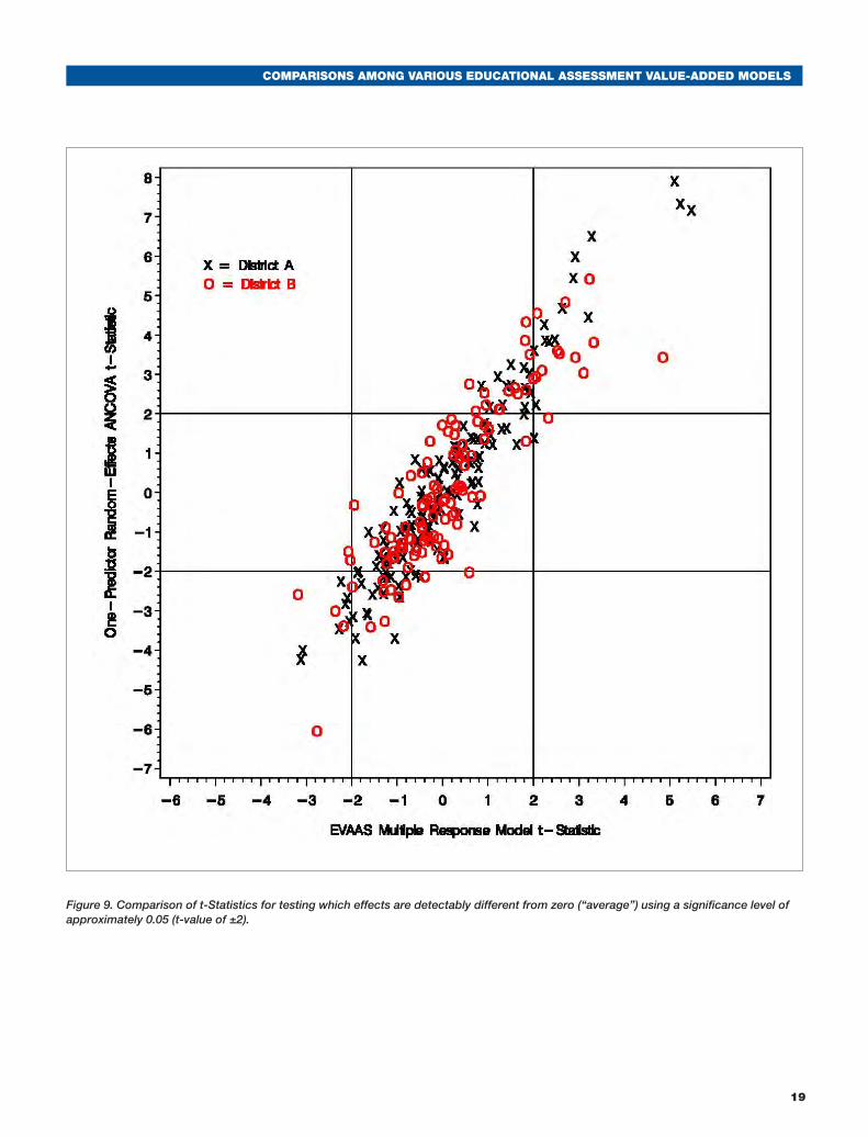
Relationship between estimates from different models. Figures 8 and 9 display the relationship between estimates from different models. These figures show values of t-statistics that test whether an effect is significantly different from zero (zero being the “average” effect for the district). Figure 5 plots the t-statistics from the Class Average Gain model versus those from the EVAAS MRM. The reference lines at plus and minus 2 correspond to commonly used decision points for identifying effects which are detectably above or below average from those that are not detectably different, corresponding to a statistical significance level of approximately 0.05.

While the estimates from different models are positive and highly correlated, there are serious differences that must be noted, which indicate that having a rather high correlation between estimates from different value-added models is totally insufficient to judge their relative equivalence. Notice in Figure 8 that the Class Average Gain model identifies many more classrooms as detectably different from average than does the MRM. Many of these are almost certainly false signals caused by the instability in the Class Average Gain estimation process. But also notice that there are indeed classrooms that are detectably Above from the MRM model that were not with the more simplistic approach. Increased reliability certainly improves the likelihood of appropriate identification.

Figure 9 shows the t-statistics from the One-Predictor Random-Effects ANCOVA versus the MRM model. There is stronger agreement here than in Figure 8, probably due to the fact that both models benefit from the stability inherent in using random effects. Nevertheless, there are still quite a few classrooms that are detectably different according to the ANCOVA but not according to the MRM model. In this case, the disagreement stems largely from the bias in the ANCOVA estimates resulting from the problem of measurement error in the predictor variable. The MRM approach yields the most conservative estimates of all of the value-added models presented herein.


11

Summary

In Table 3, the advantages and disadvantages of each of the models is summarized. Clearly, the Class Average Gain model and any of the analysis of covariance (ANCOVA) models with one score as the predictor should never be used because of the great likelihood of providing severely misleading information. Based upon our work for the past 24 years, the multivariate response model is the best that has been developed to date. It has been found to be robust under trying simulated data conditions, as well as having been used successfully in real-world applications. It gives conservative results minimizing the likelihood of both false positives and negatives.

If however, the opportunity does not exist to use this model, the second best is the univariate response model (URM). This model has many of the desirable features of the MRM but does not allow future test data to be incorporated. Thus, it does not offer the same level of protection from exogenous pulses that could affect student achievement which are outside of the control of responsible educators as does the MRM.

References

Raudenbush, S. W., and Bryk, A. S. (2002). Hierarchical Linear Models: Applications and Data Analysis Methods. Thousands Oaks, CA: Sage Publications.

Sanders, W. L., Saxton, A. M., and Horn, S. P. (1997). The Tennessee Value-Added Assessment System: A Quantitative Outcomes-Based Approach to Educational Assessment. In J. Millman (Ed.), Grading Teachers, Grading Schools: Is Student Achievement a Valid Educational Measure? pp. 137-162. Thousand Oaks, CA: Corwin Press.

Wright, S. P. (2004). Advantages of a Multivariate Longitudinal Approach to Educational Value-Added Assessment Without Imputation. Paper presented at the National Evaluation Institute, Colorado Springs, CO, July 8-10, 2004. Available at http://www.nationalevaluationinstitute.org/nei/2004/Wright-NEI04.pdf

12


District A (152 classrooms)

District B(120 classrooms)

Model No. of Students

% of Students Used

No. of Students

% of Students Used

Class Avg. Score 3,784 100.00% 2,651 100.0%

Class Avg. Gain 3,318 87.68% 2,367 89.3%

Gain as Dep. Variable, Classrooms Fixed 3,318 87.68% 2,367 89.3%

Gain Dep. Variable, Classrooms Random 3,318 87.68% 2,367 89.3%

ANCOVA, One Prev. Score, Classrooms Fixed 3,318 87.68% 2,367 89.3%

ANCOVA, One Prev. Score, Classrooms Random 3,318 87.68% 2,367 89.3%

ANCOVA, Students with 6 Previous Scores 2,869 75.82% 2,085 78.6%

EVAAS URM, ANCOVA, Nested Predictors 3,390 89.59% 2,436 91.9%

EVAAS MRM, Multivariate Longitudinal Layered Model, Uses All Student Data 3,784 100.00% 2,651 100.0%

Table 1: Number and Percentage of Students’ Scores Used with Each Model


13

Table 2. Simple Correlations Between SES Indicators and Classroom Estimates

District A (152 classrooms)

District B(120 classrooms)

Model pFRPL pNW pFRPL pNW

Class Avg. Score -0.710 -0.647 -0.773 -0.699

Class Avg. Gain -0.069 -0.125 0.133 0.138

Gain as Dep. Variable, Classrooms. Fixed -0.069 -0.125 0.133 0.138

Gain as Dep. Variable, Classrooms. Random -0.052 -0.119 0.137 0.142

ANCOVA, One Prev. Score,

Classrooms Fixed -0.540 -0.533 -0.327 -0.284

ANCOVA, One Prev. Score, Classrooms Random -0.515 -0.515 -0.306 -0.264

ANCOVA, Students with 6 Previous Scores -0.304 -0.335 -0.088 -0.043

EVAAS URM, ANCOVA, Nested Predictors -0.342 -0.370 -0.102 -0.049

EVAAS MRM, Multivariate Longitudinal Layered Model -0.368 -0.379 -0.005 0.005

14


Figure 4. Relationship between Class Average Score effects and %FRPL


15

Figure 5. Relationship between Class Average Gain effects and %FRPL

16


Figure 6. Relationship between One-Predictor Fixed-Effects ANCOVA and %FRPL


17

Figure 7. Relationship between EVAAS Multiple Response Model and %FRPL

18


Figure 8. Comparison of t-Statistics for testing which effects are detectably different from zero (“average”) using a significance level of approximately 0.05 (t-value of ±2). MRM is the EVAAS Multiple Response Model; CAG is the Class Average Gain model. NDD means “not detectably different.”


19

Figure 9. Comparison of t-Statistics for testing which effects are detectably different from zero (“average”) using a significance level of approximately 0.05 (t-value of ±2).

20


Model Advantages Disadvantages

Class Avg. Score 1. Simple to calculate. 2. All present student scores are used in

the calculation.

1. Is not a value-added measure. 2. No way to partition prior schooling

influences from the current influence.3. Severely confounded with SES effects.

Class Avg. Gain 1. Simple to calculate. 1. Only students with previous and current scores contribute to the calculations.

2. Test scales between adjacent grades must have a slope of one.

3. Standard errors of the estimates are very unstable resulting in large numbers of both false positive and negative effects.

4. No protection from spurious estimates due to the accumulation of random errors.

Gain as Dep. Variable, Class. Fixed

1. Simple model to fit with most commercially available software.

1. Only students with previous and current scores contribute to the calculations.


3. No protection from spurious estimates due to the accumulation of random errors.

Gain as Dep. Variable, Class. Random

1. Simple model to fit if software with mixed model capability is available.

2. Some protection from spurious estimates due to the accumulation of random errors.



Table 3. Summary of Comparisons Among Models


21


ANCOVA, One Prev. Score, Class. Fixed

1. Simple model to fit with most commercially available software.

2. Does not require the previous test scores to be on the same scale as the current score.

3. Relationship between the current and previous score does not have to have a slope equal to one.


2. Severe biases resulting from the errors in predictor variable problem.

3. No protection from spurious estimates due to the accumulation of random errors

ANCOVA, One Prev. Score, Class. Random






2. Severe biases resulting from the errors in predictor variable problem..

ANCOVA, for Students with 6 Previous Scores




4. Dampens the error of measurement in the predictor variable problem.


1. Severe loss of information due to the fact that many students will not have a complete resting history, raising a legitimate concern about student selection bias.

22



EVAAS URM, ANCOVA, Nested Predictors, Class. Random



3. Uses all data for each student if at least 3 prior test scores are available.

4. Minimizes the concern about student selection bias.

5. For classroom level analysis accommodates team teaching, departmentalized instruction and self contained classrooms.

1. Most commercially available software with mixed model capability can be used, but extensive programming is necessary to set the pseudo classification variables.

2. Computer resources necessary for computations are not trivial.

EVAAS MRM, Multivariate Longitudinal Layered Model

1. Uses all data for each student. 2. Eliminates the concern about student

selection bias because data from all students are included in the analysis no matter how sparse of complete.

3. Uses past, present and future data for each student.

4. Provides protection against known or unknown pulses that could provide influences on student achievement not attributable to educational intent (i.e. tornado alert, an individual failing to follow the testing rules, etc.)

5. Provides the most conservative estimates of the classroom effects.

6. For classroom level analysis accommodates team teaching, departmentalized instruction and self contained classrooms.

1. Even though the statistical methodology and theory on which this approach is based is published, at the present time commercially available software is not available to accommodate the calculations. These services are available to districts from the SAS EVAAS group.

2. Does require that the test data within a grade and subject meet a requirement that the expected amount of progress be consistent over the entire range of student achievement. If this condition is not meet with the scale scores coming directly from a test supplier, then data transformation are necessary to ensure this condition.

SAS Institute Inc. World Headquarters +1 919 677 8000To contact your local SAS office, please visit: www.sas.com/offices

SAS and all other SAS Institute Inc. product or service names are registered trademarks or trademarks of SAS Institute Inc. in the USA and other countries. ® indicates USA registration. Other brand and product names are trademarks of their respective companies. Copyright © 2010, SAS Institute Inc. All rights reserved. S56937_0510e

comparisons among various educational assessment … · white paper comparisons among various...

Documents