i

COMPARISON OF THE TWO MICRO-

SIMULATION SOFTWARE

AIMSUN & SUMO

FOR HIGHWAY TRAFFIC MODELLING

AJI RONALDO (aliro229)

TAUFIQ ISMAIL (tauis485)

2012

Linköping University

Department of Science and Technology

Intelligent Transport System

ii

iii

COPYRIGHT

The publishers will keep this document online on the Internet – or its possible replacement –from

the date of publication barring exceptional circumstances.

The online availability of the document implies permanent permission for anyone to read, to

download, or to print out single copies for his/hers own use and to use it unchanged for non-

commercial research and educational purpose. Subsequent transfers of copyright cannot revoke this

permission. All other uses of the document are conditional upon the consent of the copyright owner.

The publisher has taken technical and administrative measures to assure authenticity, security and

accessibility.

According to intellectual property law the author has the right to be mentioned when his/her work is

accessed as described above and to be protected against infringement.

For additional information about the Linköping University Electronic Press and its procedures for

publication and for assurance of document integrity, please refer to its www home page:

http://www.ep.liu.se/.

iv

ABSTRACT In order to make good decisions in transportation, decision-makers need some references to support the decision. One source for such reference is to perform a micro-simulation; a model for representing real-world conditions including the behavior of travelers, vehicles and the infrastructure. This study will examine and present a comparison between AIMSUN (a commercial micro-simulation software) and SUMO (a non-commercial micro-simulation software), identifying advantages and disadvantages of these applications in relation to the study object Södra länken, that is E266 and E75, in south part of Stockholm, Sweden.

A calibration process is conducted in order to find the best value of a set of parameters in each software. The best set of parameters will be selected based on the lowest value of a Root Mean Square Error (RMSE) computed based on observed speed data and the model output. The parameters is then validated using evening peak-hour data.

This research gave result that from the given experiments with the SUMO software, the best set of parameters was when the value of Driver Imperfection at 0,3 and Driver’s Reaction Time at 1,7. For AIMSUN , the best set of parameters was when the value of Maximum Desired Speed at 100 km/h and Speed Acceptance at 1,1.

In comparison, AIMSUN has advantages in terms of the simplicity for the user in creating network, setting the parameters and creating animation over SUMO. The complexity of the SUMO software stimulate the user to carefully build the model.

Key Word : AIMSUN, micro-simulation, software, traffic, modelling

v

vi

ACKNOWLEDGEMENT

Firstly we would like to thank to Allah The Almighty God who gives His grace and mercy so that this Master Thesis can be completed. For our supervisors Prof. Jan Lundgren and Clas Rydergren, Ph.D, we also would like to say thank you for their precious supports, guidance and advices all this time.

To our beloved family in Indonesia, who never stops giving their spirits, motivations, love and pray so that we can finishing our thesis.

Credits also given to our friends from Indonesia Catur Yudo Leksono and Tina Andriyana for their assistances in the making of our thesis as a teacher and also as a discussion partner. Special thanks for Amalia Defiani which give us extra power to finish this thesis.

The last but not the least, our gratitude is also given to MSTT UGM and Transportation Ministry of

Indonesia for the support and everything so that the education at Linköping University

accomplished.

Norrköping, June 2012

Aji Ronaldo and Muhammad Taufiq Ismail

vii

TABLE OF CONTENTS

COPYRIGHT .............................................................................................................................................. ii

ABSTRACT ............................................................................................................................................... iv

TABLE OF CONTENTS ............................................................................................................................. vii

LIST OF TABLES ........................................................................................................................................ x

LIST OF FIGURES ..................................................................................................................................... xi

LIST OF ABBREVIATION ........................................................................................................................ xiii

CHAPTER 1. INTRODUCTION .................................................................................................................. 1

1.1. BACKGROUND ......................................................................................................................... 1

1.2. AIM AND PURPOSE ................................................................................................................. 1

1.3. SIGNIFICANCE .......................................................................................................................... 1

1.4. DELIMINATION ........................................................................................................................ 1

1.5. AREA OF RESEARCH................................................................................................................. 1

1.6. STRUCTURE OF THE REPORT ................................................................................................... 3

CHAPTER 2 LITERATURE REVIEW ............................................................................................................ 5

2.1. Traffic Simulation .................................................................................................................... 5

2.2. AIMSUN ................................................................................................................................... 5

2.3. SUMO (Simulation of Urban MObility) ................................................................................... 6

2.4. MODEL CALIBRATION .............................................................................................................. 9

2.5. Previous Research ................................................................................................................. 10

2.2.1. iTetris ............................................................................................................................ 10

2.2.2. VABENE ......................................................................................................................... 10

2.2.3. CityMobil ....................................................................................................................... 11

2.2.4. VTI Comparison ............................................................................................................. 11

CHAPTER 3 INPUT DATA FOR THE SIMULATION ................................................................................... 13

3.1. Detector ................................................................................................................................ 13

3.2. Data ....................................................................................................................................... 15

3.3. Parameters of the models..................................................................................................... 19

3.3.1. Parameter in AIMSUN ................................................................................................... 19

3.3.2. Parameter of the SUMO................................................................................................ 21

CHAPTER 4 MODEL CONSTRUCTION .................................................................................................... 25

4.1. DEVELOPMENT IN AIMSUN & SUMO .................................................................................... 25

viii

4.1.1. AIMSUN ......................................................................................................................... 25

4.1.2. SUMO ............................................................................................................................ 31

4.2. CALIBRATION AND VALIDATION ........................................................................................... 35

4.2.1. CALIBRATION IN AIMSUN .............................................................................................. 35

4.2.2. Calibration of the SUMO ............................................................................................... 36

4.2.3. VALIDATION IN AIMSUN ............................................................................................... 37

4.2.4. Validation of the SUMO ................................................................................................ 37

Model Output ....................................................................................................................................... 38

CHAPTER 5 RESULT ............................................................................................................................... 39

5.1. AIMSUN ................................................................................................................................. 39

5.2. SUMO .................................................................................................................................... 46

5.3. COMPARISON AIMSUN AND SUMO ...................................................................................... 51

5.3.1. Result on Speed and Flow ............................................................................................. 51

5.3.2. Network ........................................................................................................................ 53

5.3.3. Demand ......................................................................................................................... 53

5.3.4. Control .......................................................................................................................... 53

5.3.5. Output ........................................................................................................................... 54

5.3.6. Guidance ....................................................................................................................... 54

5.3.7. Technical support .......................................................................................................... 54

CHAPTER 6 CONCLUSIONS .................................................................................................................... 56

REFERENCES .......................................................................................................................................... 58

APPENDIXES ............................................................................................................................................ a

A. SUPPLIED DEMAND DATA ........................................................................................................... a

1) Morning Demand (entrance Detectors) ................................................................................. a

2) Morning Demand (Exit Detectors) .......................................................................................... b

3) Matrix of Morning Demand (5 minutes interval).................................................................... c

Matrix of Morning Demand (5 minutes interval)............................................................................ d

4) Evening Demand (entrance Detectors) ................................................................................... e

5) Evening Demand (Exit Detectors) ............................................................................................ f

6) Matrix of Evening Demand (5 minutes interval) ..................................................................... g

Matrix of Evening Demand (5 minutes interval) ............................................................................. h

B. AIMSUN CALIBRATION ................................................................................................................. i

1) Calibration Process Entrance Detectors .................................................................................. i

ix

2) Calibration process in Exit-Detectors ....................................................................................... j

3) Comparison of Model Output and observation Speed in all detectors .................................. k

4) Validation AIMSUN Using Evening Flow Data ......................................................................... o

C. SUMO CALIBRATION ................................................................................................................... s

1) Detector 1,845 ........................................................................................................................ s

2) Detector 23,205 ....................................................................................................................... t

3) Detector 3,270 ........................................................................................................................ u

x

LIST OF TABLES Table 1. Detector inventory .................................................................................................................. 14

Table 2. OD-Matrix for morning peak-hour .......................................................................................... 15

Table 3. OD-matrix for evening peak-hour ........................................................................................... 15

Table 4. Flow number and average speed in morning peak-hour ........................................................ 16

Table 5. Flow number and average speed in evening peak-hour ......................................................... 17

Table 6. Flow number and average speed in morning peak-hour ........................................................ 18

Table 7. Flow number and average speed in evening peak-hour ......................................................... 19

Table 8. The Car-following models implemented in SUMO (9) ............................................................ 22

Table 9. Demand matrix for the first 5-minutes demand in morning .................................................. 27

Table 10. Error checking item ............................................................................................................... 31

Table 11. Parameters set in SUMO network ......................................................................................... 32

Table 12. Vehicle properties parameter value ..................................................................................... 33

Table 13. The Krauβcar-following model parameter value .................................................................. 33

Table 14. The calibration process in Detector 23, 205 ......................................................................... 36

Table 15. t-Test as validation process in detector 23.220 .................................................................... 37

Table 16. Validation process on 1.885 detector ................................................................................... 38

Table 17. RMSE matrix against morning speed data ............................................................................ 39

Table 18. Vehicle parameters ............................................................................................................... 40

Table 19. Behavior Parameter .............................................................................................................. 41

Table 20. t-Test Validation on exit detectors ........................................................................................ 42

Table 21. t-Test validation on entrance detectors ................................................................................ 42

Table 22. The Morning Calibration RMSE matrix .................................................................................. 46

Table 23. t-Test Validation against speed data ..................................................................................... 47

Table 24. t-Test Validation against flow data ....................................................................................... 47

Table 25. Comparison of validation on SUMO and AIMSUN by using evening flow data .................... 52

Table 26. Comparison of validation on SUMO and AIMSUN by using evening speed data ................. 53

xi

LIST OF FIGURES Figure 1. Area of research. (2) ................................................................................................................ 2

Figure 2.Detailed picture of research area (2) ........................................................................................ 2

Figure 3. Detailed picture (3) .................................................................................................................. 3

Figure 4. Building a network (11) ............................................................................................................ 7

Figure 5. Building trips from the OD-matrix (11,11) ............................................................................... 8

Figure 6. Detectors location .................................................................................................................. 13

Figure 7. Location of detector ............................................................................................................... 14

Figure 8.Time-series diagram ................................................................................................................ 15

Figure 9. Flow diagram (morning peak-hour) ....................................................................................... 17

Figure 10. Flow diagram (evening peak-hour) ...................................................................................... 18

Figure 11. Link-Node Diagram .............................................................................................................. 25

Figure 12. Number of lanes and the detectors ..................................................................................... 26

Figure 13. Lane Width ........................................................................................................................... 26

Figure 14. Flow fluctuation in 5-minutes interval in the morning for detector 23,205 ........................ 27

Figure 15. Speed fluctuation in 5-minutes interval in the morning for detector 23,205 ..................... 27

Figure 17. 24 morning matrixes and 24 evening matrixes.................................................................... 28

Figure 18. Traffic Demand control for Morning Demand data ............................................................. 29

Figure 19. Steps to create database storage in AIMSUN ...................................................................... 29

Figure 20. example of Replications and Average in each experiment .................................................. 30

Figure 21.Warming-up for flow stream ................................................................................................ 30

Figure 22. Behavior parameter ............................................................................................................. 31

Figure 23. Networks displayed in SUMO-GUI ....................................................................................... 32

Figure 24. Detectors placement in west section .................................................................................. 34

Figure 25. The model run in the SUMO-GUI ......................................................................................... 35

Figure 26. Graphic of RMSE in the AIMSUN .......................................................................................... 40

Figure 27. Morning Speed comparison between observation and the model output data at detector

23,205 in the AIMSUN........................................................................................................................... 41

Figure 28. Morning Speed comparison between observation and the model output data at detector

3.215 in the AIMSUN ............................................................................................................................. 42

Figure 29. Evening Flow Comparison between observation and model data at detector 23.220

(South) in the AIMSUN .......................................................................................................................... 43

Figure 30. Evening Flow Comparison between observation and the model output data at detector

1.885 (West) in the AIMSUN ................................................................................................................. 43

Figure 31. Evening Flow Comparison between observation and the model output data at detector

3.215 (East) in the AIMSUN .................................................................................................................. 44

Figure 32 Evening Speed Comparison between observation and model output data at detector

23.220 (south) in the AIMSUN .............................................................................................................. 44

Figure 33. Evening Speed Comparison between observation and the model output data at detector

1.885 (West) in the AIMSUN ................................................................................................................. 45

Figure 34. Evening Speed Comparison between observation and the model output data at detector

3.215 (East) in the AIMSUN .................................................................................................................. 45

Figure 35. Morning calibration RMSE chart of the SUMO .................................................................... 46

Figure 36. Junction no 1445695315 ...................................................................................................... 48

xii

Figure 37. Evening Flow Comparison between observation and the model output data at detector

1.885 (West) in the SUMO .................................................................................................................... 48

Figure 38. Evening Flow Comparison between observation and the model output data at detector

23.220 (South) in the SUMO ................................................................................................................. 49

Figure 39. Evening Flow Comparison between observation and the model output data at detector

3.215 (South) in the SUMO ................................................................................................................... 49

Figure 40. Evening Speed Comparison between observation and the model output data at detector

1.885 (West) in the SUMO .................................................................................................................... 50

Figure 41. Evening Speed Comparison between observation and the model output data at detector

23.220 (South) in the SUMO ................................................................................................................. 50

Figure 42. Evening Speed Comparison between observation and the model output data at detector

3.215 (East) in the SUMO ...................................................................................................................... 51

Figure 43. Comparison between SUMO and AIMSUN in Evening flow data on exit detectors ............ 51

Figure 44. Comparison between SUMO and AIMSUN in Evening speed data on exit detectors ......... 52

xiii

LIST OF ABBREVIATION

AIMSUN Advanced Interactive Micro-Simulation for Urban and Non-urban network

SUMO Simulation of Urban Mobility

PC Personal Computer

MSE Mean Square Error

RMSE Root Mean Square Error

1

CHAPTER 1. INTRODUCTION

1.1. BACKGROUND Transportation decision-making needs references as basis for decision in order to make good decisions. References which can be used include technical theories, literature studies, professional judgment or traffic simulation. Simulation is an important tool since simulation can represent a real condition into a visual model almost perfectly, and also can visually represent the effect of alternatives.

There are several micro-simulation softwares, both commercial or non-commercial, which can be used by academics or decision-makers to analyze transportation related problems. Since the softwares are built based on different theories and assumptions related to the modeling of traffic, each of these softwares have their own advantages and disadvantages and differences in outputs and results.

AIMSUN is one popular commercial micro-simulation applications which has been used frequently in the transportation research field. AIMSUN stands out for the exceptionally high speed of its simulations and for fusing static and dynamic traffic assignment with mesoscopic, microscopic and hybrid simulation – all within a single software application (1). One non-commercial micro-simulation application is SUMO (Simulation of Urban MObility) which is developed by the Institute of Transportation Systems at the German Aerospace Center.

1.2. AIM AND PURPOSE The aim of this thesis is to build, calibrate, validate two simulation models and perform experiments on a short stretch of motorway, outside of Stockholm. The purpose of the thesis is to give insights in how traffic simulation models can be used for analyzing real world traffic problems. The analysis will be based on a comparison of pros and cons of the two traffic simulation packages SUMO and AIMSUN for motorway traffic simulation. The study object is the area around E266 and E75 in the south part of Stockholm, Sweden. Input to the simulation study is data from the motorway control system (MCS) in the area.

1.3. SIGNIFICANCE This kind of study is needed in order to find out the advantages and disadvantages of two softwares related to the area of study object. Therefore in the future time, decision makers shall be able to decide which software, of SUMO and AIMSUN, that would more suitable in a situation similar to the one studied in this thesis.

1.4. DELIMINATION The limitations of the study are as follow:

1. The traffic simulation is developed based on provided data from traffic flow and speed detectors in the study area. The peak-hour data is used for building the traffic simulation model.

2. The calibration process in each software will only adjust two main parameters in order to find the best model.

1.5. AREA OF RESEARCH The area of this research is on Underground Street intersection in Stockholm. The area is the one of intersection between E266-Street and E75-Street (Södra länken). The location is a 3-approach

2

intersection which has 2-3 lane streets, as shown in figure 1. A detailed picture of the research area can be seen in figure 2 and figure 3.

Figure 1. Area of research. (2)

Figure 2.Detailed picture of research area (2)

3

Figure 3. Detailed picture (3)

1.6. STRUCTURE OF THE REPORT This report will be conducted in six chapters that represent the all of its contents. The structure is the following.

Chapter 2 describes about the description about traffic simulation classification and steps needed to build a simulation in SUMO and AIMSUN software. This chapter also describes the calibration process as a adjustment tool to find the best model from the experiments. Previous research, related to this thesis, is also included in this chapter. Chapter 3 describes the input data used in each software SUMO and AIMSUN. This chapter presents speed and flow data on morning and evening peak-hour at the detectors. The model parameters available in AIMSUN and SUMO are presented in this chapter in order to give better understanding of the softwares. Chapter 4 describes the model construction in the two softwares SUMO and AIMSUN. The model construction is described in terms of network, traffic demand and control in each software. This chapter also gives more details about how the calibration and validation processes in each software are conducted. Chapter 5 describes the finalized models for each software SUMO and AIMSUN. Root Mean Square Error (RMSE) from the calibration process, and the model output speeds and flows are also described in this chapter. Further, a general comparison of SUMO and AIMSUN in the term of Network, Demand, Control, Output, Guidance, Technical Support is presented. Chapter 6 gives the conclusions of this research including pros and cons of the two softwares SUMO and AIMSUN.

4

5

CHAPTER 2 LITERATURE REVIEW

SUMO and AIMSUN are tools that help their user to present simulation of alternatives in traffic engineering or traffic management. Result of the simulation can be good reference in policy-making of traffic in object area. This section will give better understanding for the reader about traffic simulation and the two softwares , of SUMO and AIMSUN.

2.1. Traffic Simulation In general, simulation is defined as dynamic representation of some part of the real world achieved by building a computer model and moving it through time (4). The use of computer simulation started when D.L.Gerlough published his dissertation titled “Simulation of freeway traffic on a general-purpose discrete variable computer” at the University of California, Los Angeles, in 1955 (5). In traffic research, there are four classes of the traffic models, but usually people dividing it into three, such as: a. Macroscopic simulation model

The macroscopic simulation model are based on the deterministic relationship of the flow, speed, and density of the traffic stream. The simulation in a macroscopic model takes place on a section-by-section basis rather than by tracking individual vehicles (6).

b. Meso-scopic simulation model

The mesoscopic simulation models combine the properties of both microscopic and macroscopic simulation models. Traffic flow unit in this type of simulation is individual vehicle but the movement is using the approach of the macroscopic mode. Mesoscopic simulation takes place on an aggregate level and does not consider dynamic speed/volume relationship. (6)

c. Microscopic simulation model

The microscopic model simulate the movement of individual vehicles based on car-following and lane-changing theories. Typically, vehicles enter a transportation network using a statistical distribution of arrivals (6). The microscopic model incorporate sub-models for acceleration, speed adaptation, lane-changing, gap acceptance etc., to describe how vehicles move and interact with each other and with the infrastructure (7).

2.2. AIMSUN AIMSUN is a widely used commercial transport modeling software, developed and marketed by TSS- Transport Simulation Systems based in Barcelona, Spain. Microscopic simulator and Mesoscopic simulator are the components of AIMSUN which allow dynamic simulations. They can deal with different traffic networks: urban networks, freeways, highways, ring roads, arterials and any combination thereof (8). The input data required by AIMSUN Dynamic simulators is a simulation scenario, and a set of simulation parameters that define the experiment. Based on AIMSUN Manual (8), the scenario is composed of four types of data such as: a. Network descriptions

The network is a package of links which connected each other by nodes (intersection) and may have different traffic feature. In order to build the network in AIMSUN, the user needs following data: 1) Map of the area (preferably in .DXF format) 2) Details of the number lanes for each section, reserved and side lanes.

6

3) Possible turning movement for every junction, including details about the lanes from which each turning is allowed and solid lines marked on the road surface.

4) Speed limits for every section and turning speed for allowed turns at every intersection 5) Detectors

The network consists of main and side lanes; lane identification; geometry specification; reserved lanes as part of section in the network. Another elements which might be put on the network are detectors, metering, Variable Message Sign, and pedestrian crossing. The other part that also important is node or intersection on lanes in the network.

b. Traffic control plans There are several type of traffic control taken by AIMSUN which are traffic signals, give-way signs and ramp metering. Traffic signals and give-way signs are used for junction nodes, while ramp metering is for sections that end at join node. The input data required to define the traffic control are (1) : 1) Signalized junction: location of signals, the signal groups into which turning movement are

grouped, the sequence of phases and, for each one the signal groups that have right of way, the offset for the junction and duration of each phase.

2) Un-signalized junctions : definition of priority rules and location of Yield and/or Stop signs 3) Ramp metering: location, type of metering, control parameters (green time, flow or delay

time).

c. Traffic demand data Traffic demand data in AIMSUN can be defined in two different ways, by the traffic flows at the sections or by an O/D matrix. Several O/D matrices or Traffic States will be grouped into a traffic demand. Following data must be provided for those different types of traffic demand data based on AIMSUN User’s Manual: 1) Traffic Flows

a) Vehicle type and the attributes b) Vehicle classes c) Flows at the input sections for each vehicle type d) Turning proportion at all section for each vehicle type

2) O/D Matrix

a) Centroid definition : traffic source and sinks b) Vehicle type and attributes c) Vehicle classes d) Number of trips going from every origin centroid to any destination one.

d. Public transport plans.

In order to define Public Transport, user is required to input following data: 1) Public Transport lines : a set of consecutive sections composing the route of a particular

bus 2) Reserved lanes 3) Bus stops: location, length and type of bus stops in the network. 4) Allocation of Bus Stops to Public Transport Lines 5) Timetable: departures schedule, type of vehicle and stop times.

2.3. SUMO (Simulation of Urban MObility) “Simulation of Urban MObility” is an open source, highly portable, microscopic road traffic simulation package designed to handle large road networks developed by the Institute of

7

Transportation System at the German Aerospace Center (9). SUMO is not only a traffic simulation, but rather a suite of applications which help to prepare and perform the simulation of traffic (10). In order to simulate in a proper format, “SUMO” requires the representation of road networks and traffic demand, both have to be imported or generated using different sources. SUMO allows to generate various outputs for each simulations run. The outputs are ranging from simulated induction loops to single vehicle positions.

In the SUMO, there are 4 steps needed in order to run the simulation such as: a. Building the network

Network file of the SUMO describes the traffic related part of a map. It contains the network of roads/ways, junctions/intersections, and traffic lights in a map. To build the network can be either done by generating an abstract network using NETGEN, setting up an own description in XML and importing it using NETCONVERT or by importing an existing road network using NETCONVERT. The imported existing road network can be found from non-SUMO networks such as: OpenStreetMap, VISUM, Vissim, openDRIVE, MATsim, ArcView (GIS shape-file), Elmar’s GDF and Robocup Simulation League. Although the imported network is representing the real condition of the network, SUMO users still should make some adjustments in order to find the exact condition as wanted.

Figure 4. Building a network (11)

b. Building the demand Once the network has been built, SUMO users can take a look at it using SUMO-GUI, but will not see any traffic inside it yet. Using existing OD-Matrix to fill the traffic flow in the network

8

and then convert it into traffic description is one of the ways. In the SUMO there are some methods to generate routes into the model: 1) Generating explicit routes

To describes own routes there are three possible ways, such as by hand, by using route and vehicle type distributions, and the last is by using trip definitions. By hand method is the simplest way to define own routes, but it only be possible if the number routes is not too high. In the SUMO, a vehicle consists of three parts: the vehicle type which describes the vehicle’s physical properties, a route the vehicle shall take, and the vehicle itself. Some things that should be considered when building on routes, the first thing is all the routes in the network have to be connected; secondly, the routes have to contain at least two edges; thirdly, the starting edge has to be at least as long as the car starting on it; and the last is the route file has to be sorted by starting times.

2) Using flow definitions and turning ratios

This method can be used by dynamic user assignment and alternatives route as an application for building demand by using flow definitions. This method can also be used to import demand data given by trips and flows.

3) Importing OD-matrices

To generate routes into the model, the OD-matrices cannot imported independently. So, the OD-matrix should imported along with the network. The OD-matrix/ matrices can be converted as amounts of vehicles that drive from one district to another within a certain time period. The imported routes only use data saved in VISUM/VISION/VISSIM formats. If the imported routes are not saved in these formats, there still a way to convert those (OD-matrix/matrices) into one of the supported formats, write our own reader for OD2TRIPS, or convert them into flow definitions and then give the OD-matrix/matrices DUAROUTER (dynamic user assignment and alternatives route application). How to importing OD-matrices so that it can be used to generate routes to the model is shown in figure 5.

Figure 5. Building trips from the OD-matrix (11,11)

4) Using random routes It is said that the random routes are the easiest, but also the most inaccurate way to feed the network with vehicle movements.

9

c. Computing the dynamic user assignment (if needed)

In order to know which routes taken by the driver in the simulation, dynamic assignment is used. There are also some others use of dynamic user assignment, to detect how is the mean speed of the lane, how much flow over the network, to solve the congestion problem, etc.

d. Performing the simulation The network file, the information of routes that will be used in the simulation and the period of time that will be used in the model are essential to run the model. If one of them is not applied in the model, the model will not be run properly.

2.4. MODEL CALIBRATION The calibration is become most important tool in finding the best model from the two softwares. Result from the calibration will determine the best value of the model parameters. The model simulation using those value of parameters will generate output which then will be used in validation process. Comparison between the model result and the real data which are taken from the field by comparison test will use 95% probability. Calculated prediction output from both AIMSUN and SUMO are used to test observed real word data. This thesis is using Excel to conduct all of statistical calculation in order to find whether the simulation will be considered as good-representing simulation or not. CALIBRATION This research using Mean Square Error (MSE) analysis to calibrate data between the model output and observation data to find optimal value of parameters in the model development. Based on “Traffic Analysis Toolbox Volume III” (12)the formula for the calibration is :

(1.1)

Where: MSE = Mean Square Error = 5-minutes interval = Detector = Model estimate of speed at detector and -th time = Observation data of speed at detector and -th time = Number of ime intervals D = Number of detector In the AIMSUN and SUMO calibration, speed data is used to find optimal value of parameters. Since the research decide to develop the model for 2-hours peak period and also use 5 minutes time interval to measure the average speed, so 24 5-minutes time-interval for 2 hours observation data is made. The lowest number MSE will take from several experiments on each set of parameters value. Based on the equation, since the calibration will use speed data then the result from this equation will have km2/h2 as unit (quadratic function). In order to make it back to the single function, RMSE (Root Mean Square Error) (13)has been used as shown on equation 2 .

(1.2)

10

The value of RMSE then will become the main criteria from choose the best set of parameter from experiments on each set of parameter.

VALIDATION In order to compare the data of scenario which is defined as (µx) with the mean of the existing validated model data (µy), following hypothesis need to be checked

Where:

= average of observed data = average of model output

will be rejected if

Where :

(1.3)

(1.4)

When rejected, its mean that the model output cannot representing the observed data. When accepted, its mean that the model output can represent the observed data.

2.5. Previous Research There are several previous research about the two softwares SUMO and AIMSUN. Those researches will give the reader better understanding and information about another usefulness of those software to solve the problems.

2.2.1. iTetris V2X communication is a technology invented to be applied in cars so that the cars can communicate with the traffic network. These days, the use of V2X communication is increasing in many countries. However, the price and the risk is too high to implement such system. Therefore a simulation is needed in order to measure the benefits of a system before it is deployed into the real world. The aim of iTETRIS project was to develop such framework and to couple the communication simulator ns3 and SUMO using an open source system called “iCS” – ITETRIS Control System which was developed within the project (14). The iCS is responsible for starting the named simulators and additional programs which simulate the V2X applications. It is also responsible for synchronizing the participating simulators, and for the message exchange. Using this simulation framework it was possible to investigate the impacts on V2X communication strategies.

Within the project several traffic management strategies were simulated e.g. prioritization of emergency vehicles at controlled intersections (15)and rerouting vehicles over bus lanes using V2X communication (16).

2.2.2. VABENE For every big city, the need of good traffic condition is essential. When a big event or a disaster happens, traffic jams will occur and it will have a great impact to the transport systems and may jeopardize the people who live in the city. The institutions responsible for the traffic should take proper actions to overcome the worst case. The objective of VABENE is to implement a system which supports the public authority to decide which action should be taken (14).

11

This project is focusing on simulating the traffic condition of large cities. In order to simulate Munich city traffic, the mesoscopic traffic model was implemented into SUMO which is available for internal proposes only. This system was used during pope’s visit in Germany in 2005 and during the FIFA World Cup in 2006.

2.2.3. CityMobil To evaluate the changes in vehicle or driver behavior of large scale effects, microscopic traffic simulations can be used. In past time, that condition was examined with the help of SUMO in the EU project CityMobil where different scenarios of (partly) automated cars or personal rapid transit were set up on different scales, from a parking area up to whole cities (14).

In this study, the evaluation of the benefits of an autonomous bus system was performed. Furthermore, scenario being applied in this study is the information of passengers waiting and route adaption to the demand given to the busses. The investigation regarding the influence of platooning vehicles on a large scale also implemented, where a middle-sized city with 100.000 inhabitants were used as the model. Those two simulations were showing good result of the transport automation.

2.2.4. VTI Comparison Swedish National Road Administration perform a research that comparing the Car-following models from traffic simulation softwares which are AIMSUN, MITSIM, VISSIM, and Fritzsche. The diiferences between the Car-following model used in these versions and the Fritzsche car-following model is however unknown (17). The Fritzsche and VISSIM have similar approach, but AIMSUN and MITSIM have different approaches. Results from those models are show similarities even though have different car-following approaches.

12

13

CHAPTER 3 INPUT DATA FOR THE SIMULATION Flow as input data is extracted from detectors on study area. Each detector in this area have its own flow data in 1-minute interval. These detectors also contain the speed average of vehicles in 1-minute intervals. The location of each detector, the speed and flow data from these detectors will be described in this chapter.

3.1. Detector There are several detectors placed around the area, figure 6 show the detector spots of the intersection street E75 and E266. The numbers shown in figure 6 represent the stationary location of the detector, each stationary location have 1-4 detectors depends on the number of lanes.

E75

E75

Yellow and purple circle in figure 6 represent the detector that be used in this research. Those detector have different role in the micro-simulation model development depends on the direction of traffic movement. By considering the detector which been marked by yellow circle as the border, the total number of detectors is 85. In order to develop the micro-simulation in this research, this research using data from 29 detectors within this area as input and validation data.

Based on the needs of data input, it was decided to choose several detectors data as input and validation data for the micro-simulation model that would be created by using AIMSUN and SUMO. The detector number that will be used in this research are shown in table 1 and to ease for understanding the situation about research area, a simple picture of detector location/point in figure 7 is created. The data taken from 00.00 to 18.24 (GMT+1) at 16th of March 2010.

The number inside the box represents stationary point associated with the table 1 below. The yellow boxes represent the detectors whose data will be used as input for this micro-simulation development. Figure 7 describe about the position of each detectors according to table 1.

Figure 6. Detectors location

14

Table 1. Detector inventory

No Stationary point Quantity Detector Numbering Role

1 1.845 3 49,50,51 Main Input

2 23.205 2 49,50 Main Input

3 3.270 4 49,50,51,52 Main Input

4 2.300e 1 49 Proportion Input for 1.845

5 23.495 1 49 Proportion Input for 23.205

6 3.015h 1 49 Proportion Input for 3.270

7 23.49 1 49 Proportion Input for 23.205

8 1.885 3 49,50,51 Validation point

9 3.215 4 49,50,51,52 Validation point

10 23.220 2 49,50 Validation point

11 2.170 4 49,50,51,52 Proportion input for 1.885

12 2.750e 1 49 Proportion input for 23.220

13 2.370h 1 49 Proportion Input for 23.220

14 23.865r 1 49 Proportion Input for 3.215

Those detectors have different role in data extraction. Table 1 shows the different role of those detectors. Main input means that the flow extracted from related points will become the basic of the calculation for determine the O/D matrix. Proportion input means that the flow extracted from related points became the tool to know the flow proportion in other direction. For example, In order to get the number of flow for West-to-East direction, the flow is taken from the flow in detector 1.845 minus the flow in detector 2.300e. Similar role as main input is given to the validation point, the difference is on the purpose of data. The flow extracted from validation point would be used for validation process while main input will be used for the calibration process.

23.220

3.215

1.885 3.270

23.205

1.845

23,490

2.370h

3.015h

2.300e

2.750e 23.495r

23.865

2.170

South

East West

Figure 7. Location of detector

15

3.2. Data Based on the supplied data, the research chooses 2 peak hour in this micro-simulation as morning and evening peak hour. For the peak hour in the morning 06.30 - 08.30 was chosen and for the evening peak hour is between 13.30 - 15.30. This duration was chosen based on the flow profile in this location as shown on figure 8.

Figure 8.Time-series diagram

Based on this characteristic, data from all selected detectors during the peak hour (06.30 - 08.30 and 13.30 - 15.30) was taken as main data for this micro-simulation development. Data in detector number 2.305; 1.845 and 3.270 are used as demand input in micro-simulation program. Detector number 2.300e; 23.495; 23.490 and 3.015h (in figure 7) is used to determine the proportion of flow in each direction. As a result from this extraction, the OD-matrix is found for both peak hour morning and evening for each direction in following table 2 and 3. Table 2 and 3 represent the traffic flow condition on peak-hour in the area for 2 hours duration.

Table 2. OD-Matrix for morning peak-hour

OD East South West

East - 1402 4096

South 1924 - 1813

West 5540 275 -

Table 3. OD-matrix for evening peak-hour

OD East South West

East - 1327 4474

South 1194 - 867

West 5665 545 -

0

1000

2000

3000

4000

5000

6000

7000

1

9

17

25

33

41

49

57

65

73

81

89

97

10

5

11

3

12

1

12

9

13

7

14

5

15

3

16

1

16

9

17

7

18

5

19

3

Nu

mb

er

of

veh

icle

s (u

nit

)

Set of time series

Flow Diagram (time series)

Flow

16

It should be noted that the data in table 2 and table 3 will not used as input in the two softwares SUMO and AIMSUN. The data in table 2 and 3 will be divided into 5-minutes interval O/D matrix and will be used as demand input which represents the traffic movement within the intersection. Further, based on this number of demand and the parameter, the traffic model will be created to represent the real condition of traffic.

Table 4. Flow number and average speed in morning peak-hour

Time

Detector

23.205 1.845 3.270

Flow Speed Flow Speed Flow Speed

6:30:00 - 6:35:00 130 67.36 320 72.94 314 65.25

6:36:00 - 6:40:00 153 64.4 255 73.53 296 67.5

6:41:00 - 6:45:00 156 64.1 291 71.93 293 56.65

6:46:00 - 6:50:00 172 61 300 73.60 292 37.3

6:51:00 - 6:55:00 162 64.3 262 73.53 291 36

6:56:00 - 7:00:00 170 63.3 261 72.33 292 36.9

7:01:00 - 6:05:00 175 62.4 267 70.33 309 37.7

7:06:00 - 7:10:00 152 60.4 239 72.13 252 33.05

7:11:00 - 7:15:00 139 61.7 240 71.47 212 27.55

7:16:00 - 7:20:00 174 60.7 254 70.67 198 29.1

7:21:00 - 7:25:00 166 59.6 257 70.40 199 29.65

7:26:00 - 7:30:00 143 60.4 269 67.80 249 28.7

7:31:00 - 7:35:00 139 64.3 272 69.47 212 28.65

7:36:00 - 7:40:00 170 61 262 71.13 213 30.9

7:41:00 - 7:45:00 138 62.9 275 70.67 175 25.35

7:46:00 - 7:50:00 152 61.3 287 67.73 167 28.1

7:51:00 - 7:55:00 142 61.9 242 71.67 261 28.15

7:56:00 - 8:00:00 160 60.6 247 70.13 180 25.65

8:01:00 - 8:05:00 152 60.3 243 71.93 168 29.45

8:06:00 - 8:10:00 152 61.7 222 50.40 165 37.2

8:11:00 - 8:15:00 149 61.5 147 20.60 240 30.7

8:16:00 - 8:20:00 137 63.5 144 20.40 133 23.15

8:21:00 - 8:25:00 141 62.9 135 18.33 214 31.25

8:26:00 - 8:30:00 119 63.4 124 18.80 173 29.9

Total 3643 5815 5498

The OD-matrix in table 2 is created based on the total number of flow in table 4 and table 6. It is implied from table 2 that 25.5% flow from East-section go to the south-section and rest of them go to the west. It also can be implied that 95.3% traffic flow from the west go to the east and 51.5% traffic flow from the south-section go to the East-section. Similar with the table 2, table 3 is created based on the flow number in table 5 and table 7. In the evening peak-hour there are no significant different. Flow percentage of traffic flow from East-to-West section and South-to-East section are bigger that morning peak-hour, but for the West-to-East section traffic flow is smaller that morning (91.2%).

17

Figure 9. Flow diagram (morning peak-hour)

Table 5. Flow number and average speed in evening peak-hour

Time

Detector

23.205 1.845 3.27

Flow Speed Flow Speed Flow Speed

13:30:00 - 13:35:00 74 64.5 311 68.22 260 67.5

13:36:00 - 13:40:00 69 64 235 70.53 230 69.65

13:41:00 - 13:45:00 71 63.1 259 67.53 243 67.8

13:46:00 - 13:50:00 75 66.2 245 69.40 236 68

13:51:00 - 13:55:00 98 64.3 243 68.47 228 76.7

13:56:00 - 14:00:00 84 65.6 250 69.07 235 76.45

14:01:00 - 14:05:00 78 65.1 228 70.93 229 68.05

14:06:00 - 14:10:00 71 65.7 247 68.07 231 67.6

14:11:00 - 14:15:00 85 65 268 68.80 257 76

14:16:00 - 14:20:00 99 64 249 71.60 253 77.15

14:21:00 - 14:25:00 87 65.1 243 70.40 237 67.55

14:26:00 - 14:30:00 85 65.3 258 69.13 248 68.45

14:31:00 - 14:35:00 74 65.3 260 68.53 241 67.4

14:36:00 - 14:40:00 105 64.3 254 69.20 240 65.95

14:41:00 - 14:45:00 88 62.5 260 67.67 277 67.45

14:46:00 - 14:50:00 110 62 248 68.73 224 77.65

14:51:00 - 14:55:00 88 66 297 66.27 231 69.5

14:56:00 - 15:00:00 63 84.6 279 62.67 254 67.7

15:01:00 - 15:05:00 96 66.9 313 64.27 306 64.5

15:06:00 - 15:10:00 119 65.2 304 57.87 285 65.8

15:11:00 - 15:15:00 100 62.7 311 42.53 264 67.4

15:16:00 - 15:20:00 90 63.8 292 34.13 286 65.2

15:21:00 - 15:25:00 109 65 291 36.60 306 65.05

15:26:00 - 15:30:00 65 43.33

2018 6210 5801

0 50

100 150 200 250 300 350

Flo

w (

un

it)

flow diagram (morning peak-hour)

Detector 2,305 Flow

Detector 1,845 Flow

Detector 3,270 Flow

18

Figure 10. Flow diagram (evening peak-hour)

Table 6. Flow number and average speed in morning peak-hour

Time

Detector

2300e 23.495 3.015h 23.49

Flow Speed Flow Speed Flow Speed Flow Speed

6:30:00 - 6:35:00 11 72.00 76 67.5 51 76.33 65 68.2

6:36:00 - 6:40:00 9 66.00 72 67.8 40 76.6 90 65.8

6:41:00 - 6:45:00 11 70.00 71 66.2 48 73.4 77 66

6:46:00 - 6:50:00 4 73.00 98 63.6 63 73.2 76 66.2

6:51:00 - 6:55:00 14 74.00 93 64 52 71.2 84 64.4

6:56:00 - 7:00:00 25 71.00 98 63.2 57 72.6 68 67.2

7:01:00 - 6:05:00 23 68.50 93 65.2 56 73.4 81 64.4

7:06:00 - 7:10:00 11 74.00 83 65.4 66 69.2 75 64.2

7:11:00 - 7:15:00 11 70.00 74 62.2 65 63.4 70 61.6

7:16:00 - 7:20:00 8 73.00 88 63 62 68.8 81 63

7:21:00 - 7:25:00 0 0.00 73 64.6 67 67.6 91 60.4

7:26:00 - 7:30:00 0 0.00 91 62.6 67 65.4 75 62.2

7:31:00 - 7:35:00 22 67.33 71 68.4 63 62.2 70 66

7:36:00 - 7:40:00 11 75.00 88 60.2 65 66.2 78 63.8

7:41:00 - 7:45:00 14 69.50 75 65.4 66 62.2 73 63.8

7:46:00 - 7:50:00 5 68.00 90 63 69 63.8 67 64.2

7:51:00 - 7:55:00 4 74.00 69 64.6 63 64.2 77 63

7:56:00 - 8:00:00 15 69.00 64 64.2 60 63 92 61.8

8:01:00 - 8:05:00 7 74.50 95 60 54 66.2 71 62.2

8:06:00 - 8:10:00 12 62.00 81 63 59 61.8 72 63.8

8:11:00 - 8:15:00 10 59.50 81 62.4 58 65.8 66 62.8

8:16:00 - 8:20:00 23 58.25 65 63.4 55 63.4 81 62.4

8:21:00 - 8:25:00 17 63.50 71 63.4 52 67 74 60.2

8:26:00 - 8:30:00 8 62.50 64 64.2 44 66 59 63.4

Total 275 1924 1402 1813

0 50

100 150 200 250 300 350

Flo

w (

un

it)

Flow diagram (evening peak-hour)

Detector 2,305 Flow

Detector 1,845 Flow

Detector 3,27 Flow

19

Table 7. Flow number and average speed in evening peak-hour

Time

Detector

2300e 23.495 3.015 23.49

Flow Speed Flow Speed Flow Speed Flow Speed

13:30:00 - 13:35:00 25 66.20 47 66 49 71.2 38 71.1

13:36:00 - 13:40:00 25 69.25 45 65.6 44 72.4 30 67.6

13:41:00 - 13:45:00 28 66.50 44 65.4 66 71.4 39 69.8

13:46:00 - 13:50:00 10 68.50 45 67.8 53 71.8 31 69.6

13:51:00 - 13:55:00 13 70.50 53 65 60 71.4 44 67.4

13:56:00 - 14:00:00 7 66.00 50 66.8 53 73.4 33 70

14:01:00 - 14:05:00 12 66.00 53 66 44 75.8 25 68.2

14:06:00 - 14:10:00 11 68.00 40 65.2 42 76.2 36 68.2

14:11:00 - 14:15:00 23 72.33 61 64.4 63 72 23 67.8

14:16:00 - 14:20:00 18 70.33 51 65 63 74.2 48 65.8

14:21:00 - 14:25:00 28 70.25 53 66 57 72.8 36 69.4

14:26:00 - 14:30:00 30 68.00 61 64.6 65 75 28 68.6

14:31:00 - 14:35:00 12 66.50 36 67 50 73.4 44 69.2

14:36:00 - 14:40:00 20 71.25 56 64.2 62 69.6 46 67.4

14:41:00 - 14:45:00 23 68.00 54 64.2 66 73.6 39 66.6

14:46:00 - 14:50:00 19 69.67 60 63 54 72 47 66,4

14:51:00 - 14:55:00 35 69.25 36 69.8 60 71.8 38 66.8

14:56:00 - 15:00:00 29 70.00 49 64.6 62 70.8 26 69

15:01:00 - 15:05:00 18 69.50 48 67 63 71.4 44 71.2

15:06:00 - 15:10:00 31 68.25 63 63.6 67 74 61 67.6

15:11:00 - 15:15:00 59 63.50 69 63.8 61 75.6 36 69

15:16:00 - 15:20:00 23 69.00 49 66.6 57 71.2 41 68.6

15:21:00 - 15:25:00 46 63.25 71 63.2 66 72.2 34 67.4

Total 545 1194 1327 867

3.3. Parameters of the models The model contains several parameters that will influence the output of the model. This section will describe about what kind of parameters that will be used in the two softwares SUMO and AIMSUN.

3.3.1. Parameter in AIMSUN Vehicle Parameters Vehicle characteristic of vehicle are include length, power ratio and it width. Higher power ratio on a car can be used in the special condition such as overtaking condition, in which car driver tend to give bigger power ration or acceleration. Based on AIMSUN Manual (1) Vehicle parameters are included:

a) Width (meters) This parameter is only for graphical purpose and does not have a direct influence on the modeling of traffic.

20

b) Maximum desired speed (km/h) Maximum speed of the type of vehicle can travel at any point in the network.

c) Maximum acceleration (m/s2) Maximum acceleration that can achieved by vehicle at any circumstance

d) Normal deceleration (m/s2) Maximum deceleration of vehicle under normal circumstances (as used in the Gipps’ car-following model).

e) Maximum deceleration (m/s2) It can be considered as most severe breaking that can apply under special circumstances.

f) Speed acceptance This parameter (θ>0) can be interpreted as the “level of goodness” of the drivers or the degree of acceptance of speed limits. θ > 1 means that the vehicle will take as maximum speed for a section a value greater than the speed limit, while θ< 1 means that the vehicle will use a lower speed limit. See the next section for details on how maximum desired speed for a vehicle is calculated for different parts of the network (1).

g) Minimum distance between vehicles (meters) A vehicle will keep this distance between itself and preceding vehicle when stopped.

h) Maximum give-way time This parameter applies either the normal gap-acceptance model or the lane-changing model in order to cross or merges with traffic.

i) Guidance acceptance, This parameter (0 ≤ λ ≤ 1) gives the level of compliance of related vehicle type with the guidance indication.

Driver Parameter The model also will use driver behavior to determine which the model is fit to the real condition. Parameters applied for driver parameter are:

a) Driver's reaction time Driver's reaction time is the time that used by the driver to react to speed change in the preceding vehicle. Reaction time can be either Fixed (equal to Simulation Step) or Variable (multiple of Simulation Step). In Fixed type, the values are same for all vehicles. In Variable type, the user can define a discrete probability function for each vehicle type (18).

b) Reaction time at stop Reaction time at stop is the time taken for a stopped vehicle to react to the vehicle acceleration in front or to the light traffic changing to green. This parameter has a strong influence in the queue discharge behavior.

c) Queuing Up Speed This is the threshold of vehicle’s speed value (m/s). If any vehicle’s speed decrease below this threshold, then it will be considered stopped and join the queue.

21

d) Queuing Leaving Speed This is the threshold value of vehicle’s speed (m/s). If any stopped-vehicle speed in a queue increases above this threshold value, then it will be considered left the queue and no longer to be at a standstill.

e) Car-Following model, The car-following model used in AIMSUN is based on the Gipps model which basically consists of two components, which are acceleration and deceleration. Acceleration represent the vehicle intention to reach a certain point of speed (desired speed), and Deceleration represent the limitation imposed by the preceding vehicle when trying to drive on the desired speed (1).

2-lanes Car-Following parameters used in this model are: a) Number of vehicles Maximum number of vehicles in the 2-lane variation of the Car-Following Model, which is used for modeling the influence of adjacent lanes in the Car-Following Model.

b) Maximum Distance, Maximum distance ahead to be considered in the 2-lane Car Following Model.

c) Maximum Speed difference, Maximum speed difference between one lane and the adjacent lane in the 2-lane Car Following Model.

d) Maximum Speed difference On-Ramp Maximum speed difference between the main lane and an on-ramp lane in the 2-lane Car following Model.

Lane Changing Parameters Percent overtake This parameter represents the percentage of the speed from which a vehicle decides to overtake. The value has to be greater than zero and less than or equal to one

Other global parameters Road side of vehicle movement The effect of this parameter on simulation result varies, depending on the geometry and type of the network, but it always affects the behavior of the vehicles.

3.3.2. Parameter of the SUMO Vehicle Parameters a) Vehicle Properties Vehicles used in the model should be defined whether is it a passenger car, truck, or bus. To define what kind of vehicle used in the SUMO, some vehicle properties have to be set first. The vehicle properties were set in the flow file and the parameters to be set on that property are:

a. id – the name of the vehicle type; b. length – the vehicle’s netto-length (m); c. miniGap – empty space after leader (m); d. maxSpeed - the vehicle’s maximum velocity (m/s); e. guiShape – how this vehicle is rendered; f. guiWidth – the vehicle’s width (m).

22

b) Routes The parameters used in route path and flow proportion are:

a. id – the name of route in certain interval; b. from – the name of the edge which is route started; c. to – the name of the edge which is route ended; d. Number - the number of vehicles generated in the model; e. type – the name of vehicle types;

c) Car-Following model The car-following model describes that the speed of following car is influenced by the acceleration of the preceding car , which can be described best by the following equation:

: speed of vehicle n : speed of succeeding vehicle n : driver’s reaction time (s)

The equation above was first proposed by Pipes as cited in Krauss, 1998 (19). In the SUMO, the car-following models implemented:

Table 8. The Car-following models implemented in SUMO (9)

Element Short Name Description

1. carFollowing-Krauss

2. carFollowing-KraussOrig1

3. carFollowing-PWagner2009

4. carFollowing-BKerner

5. carFollowing-IDM

SUMOKrauβ SKOrig PW2009 Kerner IDM

The Krauβ-model with some modifications which is the default model used in SUMO The original Krauβ-model A model by Peter Wagner, using Todosiev’s action points. A model by Boris Kerner Note: currently under work The Intelligent Driver Model by Martin Treiber Note: Problems with lane changing occur

In SUMO, the SUMOKrauβ model is used. This model is a modification of the original Krauβ model. Basically, the Krauβ model can be formulate as follow (19):

Where,

23

The index vn is the notation of vehicle’s position where the leading vehicle always has bigger value than the following. The gap or distance between two vehicles denoted as , desired gap or expresses how long the gap between vehicles can be achieved, vehicle desired speed or shows how large the driver can run the vehicle with maximum speed, time step or is assumed has the same value or equal to the driver’s reaction time, time scale is defined as

where it has the same value with

. Here the random perturbation has been introduced to

allow for deviations from optimal driving. has the same value with εa, where ε is having value between 0 and 1. The maximum acceleration (a), deceleration (b), and jammed spacing (l) are assumed constant.

The parameters used in the SUMO Krauβ model are: a. accel– acceleration ability [m/s2], b. decal – deceleration ability [m/s2], c. sigma – driver imperfection (real value between 0 and 1 inclusive), d. tau – driver’s reaction time *s+, e. minGap – gap between preceding and following cars [m].

Vehicles and Routes a) Repeated vehicles It is possible to define repeated vehicle flows, which have the same parameters as the vehicle except for the departure time. The id of the created vehicles is "flowId.runningNumber" and they are distributed equally in the given interval. The following additional parameters are known:

a. begin – first vehicle departure time [s], b. end – end of departure interval [s], c. vehsPerHour – number of vehicles per hour (not together with period) [h], d. period – repetition period (not together with vehsPerHour) [s], e. number – total number of vehicles [#].

b) Routes Each route has its own class and to differentiate one to others, it colored with different color in the map. As well as in the SUMO, to distinguish one route to another, it gives attributes to the route such as id (the name of the route), color (the route’s color) and edges.

A vehicle’s depart and arrival parameter To control how a vehicle is inserted into the network and how it leaves it, SUMO needs to add some parameters such as:

a. departLane – the lane on which the vehicle shall be inserted. b. departPos – the position at which the vehicle shall enter the network [m], c. departSpeed – the speed with which the vehicle shall enter the network [m/s] d. arrivalLane – the lane at which the vehicle shall leave the network, e. arrivalPos – the position at which the vehicle shall leave the network [m], f. arrivalSpeed– the speed with which the vehicle shall leave the network [m/s].

Stops In some case e.g. at signalized intersections, roundabout, etc. drivers have to stop their car in order to give way to other drivers for a couple of seconds or minutes. As if in the modeling like SUMO, vehicles may be stop for a defined time span or wait for persons by using the stop element either as part of a route or a vehicle.

Lane Changing Parameters In the SUMO version 0.15.1, parameters such as the lane change model, and others, are not directly accessible to a user in configuration files. Therefore, the parameters mentioned before were not

24

considered during the calibration process. For vehicle and driver parameters of the car following model, special attentions is given to:

a. accel – acceleration ability [m/s2] b. decal – deceleration ability [m/s2] c. sigma – driver imperfection (real value between 0 and 1 inclusive), d. length – vehicle length (increased by a typical gap distance between stopped vehicles) [m], e. maxspeed – vehicle maximum velocity [m/s],

25

CHAPTER 4 MODEL CONSTRUCTION

4.1. DEVELOPMENT IN AIMSUN & SUMO There are several elements that needed to construct a model in both software SUMO and AIMSUN. This section will explain about each element included in each software in order to make the model.

4.1.1. AIMSUN

LINK-NODE DIAGRAM Network development can be done by using GUI (Graphical User Interface) which facilitated by AIMSUN itself. Generally, there are 6 links, 4 nodes and 3 centroids in this network as shown in figure 10 below.

Centroid

345

Centroid

346

Centroid

347

Figure 11. Link-Node Diagram

GUI in AIMSUN made user can directly build and modified the network as closely as possible to the real traffic condition. Actually, the network can be considered as 3-approachment intersection but with different stage of lane. The directions are coming from south, east, and west.

LINK GEOMETRY DATA a) Number of Lane There are different numbers of lane within links in this network. For link from west to east (E75), the number of lane change 3 times. At the beginning (from west) the road has 3 lanes, but since there is diverging link the number of lane reduced into 2 lanes. About hundred meters before merging lane, the number of lane of this link increased into 3 lanes and then increased again into 4 lanes after there is merging lane from south direction. All links which directly connected to East-centroid have 4 lanes road. All links which directly connected to the west-centroid are 3-lanes-roads for and 2-lanes-road for all links which directly connected to south-centroid. Figure 11 shows about the number of lane in study area.

26

Figure 12. Number of lanes and the detectors

b) Lane width Most part of the network is in the tunnel. In main tunnel, lane width is 3.75 m and at the ramps 4.5 m. Specific dimension for the road in the main tunnel is 0.75 m for left shoulder; 3.75 m for main lane and 1.75 m for the right shoulder. For the ramp part, the specific dimension is 2.5 m for left shoulder; 4.5 m for main lane and 1 m for right shoulder. The dimension can be seen at figure 12 . Along the network there are no pedestrian crossing facilities, bus stop, or reserved lane for public transport. Detail picture of lane width in “on ramp” and “main tunnel” can be seen in figure 12 below.

2,5 m4 m

1 m

0,75 m

3,75 m 3,75 m

1,75 m

ON RAMP LANE

MAIN TUNNEL LANE

LEFT SHOULDER LANERIGHT

SHOULDER

LEFT SHOULDER LANE LANE RIGHT SHOULDER

Figure 13. Lane Width

= Main detectors

27

TRAFFIC DEMAND DATA Since the supplied data do not mention about the type of the car, every vehicle counted on related detector are considered as private car. 24 demand matrix was used on the morning as traffic demand input in order to get the real fluctuation as the real condition. Each matrix is a 5-minutes flow aggregation for all direction. Table 8 shows about demand matrix for the first 5-minutes from 2 hours demand which become input for the model. Graphic in figure 11 shows about the fluctuation of demand in 5-minutes interval which covered by detector 23,205. It can be implied that O/D-matrix in table 8 give a contribution on the first point in figure 13.

Table 9. Demand matrix for the first 5-minutes demand in morning

O/D West East South

West 0 309 11

East 263 0 51

South 54 76 0

Figure 14. Flow fluctuation in 5-minutes interval in the morning for detector 23.205

The flow data are subtracted from the counting of 14 different detectors. Each detector also count the average spot speed in 1 minute interval. For analysis purpose, those speeds were broke down into 5-minutes average speed. Figure 14 shows speed average in 5-minutes interval on detector 23.205.

Figure 15. Speed fluctuation in 5-minutes interval in the morning for detector 23.205

0

20

40

60

80

100

120

140

0 5 10 15 20 25

Flo

w (

veh

)

Time series (5 minutes)

detector 23.205 (enterance)

Observation

0

20

40

60

80

100

0 5 10 15 20 25

Spe

ed

(km

/h)

Time series (5 minutes)

detector 23,205

Observation

28

SIMULATION CONTROL DATA a) Scenario In order to run the simulation, Dynamic Scenario has to be created. Each Dynamic Scenario contains traffic demand that will be used in every experiment on the same scenario. The user has to determine what kind of traffic demand will be used. In each Dynamic Scenario also determine where the result will be saved as database, and how long the interval of the result will be generated. A Dynamic Scenario can hold 15-19 experiments. Figure 15 shows the user interface in AIMSUN where the user shall select the “traffic demand”.

Figure 16. Scenario control interface in AIMSUM

b) Traffic Demand Control Data Traffic demand as mentioned in previous part has important part in the modeling process. The demand will determine the result of the model in the end. This analysis covered 2 hours demand with 5-minutes interval of flow, which means 24 matrixes of 5-minutes interval flow as seen in table 8 for morning demand control and the other 24 for evening demand control (figure 16).

Figure 17. 24 morning matrixes and 24 evening matrixes

In AIMSUN, all 24 matrixes of morning demand will combine each other in Traffic Demands control as seen in figure 17.

29

Figure 18. Traffic Demand control for Morning Demand data

c) Database Each scenario has to be connected to one database file as data storage. Scenario and database are connected by QODBC driver. Every QODBC driver has several connections and each connection have its own database. In every scenario, the user has to determine the QODBC connection to keep the result of each replication in each experiment. Figure 18 shows steps to create database storage connection in AIMSUN.

Figure 19. Steps to create database storage in AIMSUN

30

d) Experiment Each experiment has different set of parameter value. 10 replications were created on each experiments and 1 average that will be calculates the average of those 10 replications. In order to make it easier to find the data and to remind experiment that have been done, each experiment was renamed based on the number or value of parameters that changed in each experiment. Right part of figure 19 shows an example about “experiment” in AIMSUN.

Figure 20. example of Replications and Average in each experiment

The number of “average” replication has to recorded for each experiment to ease for finding the data in database. In each experiment, value of behavior parameters were set as default (figure 21) and put 15 minutes as warming-up of flow stream (figure 20).

Figure 21.Warming-up for flow stream

31

Figure 22. Behavior parameter

Options such as applying the 2-lane car following model, warm-up time, and reaction time, lane-changing (figure 21) have to be performed in each experiment .

Table 10. Error checking item

No Item Access

1 2 3 4 5 6

Network Demand Data Vehicle Parameter Behavior parameter Database Connesction Number of Replication

GUI Demand option Vehicle option Experiment option Scenario option Experiment Option

When the entire item above checked by user, a proper simulation or experiment can be performed using parameters which decided to be taken at the beginning of each simulation.

4.1.2. SUMO

Network A network is very essential in building a traffic simulation, because it is the core or the foundation of the model itself. Without the existence of a network, the traffic simulation model cannot be run. In the SUMO, there are two ways to build a network such as: a) Writing our own network on XML-descriptions; and b) Importing from non-SUMO networks.

In this thesis, non-SUMO networks was used to create the networks. The non-SUMO networks being used as the base of the networks is coming from OpenStreetMap file. Due to the true nature of the studied location are arterial roads, set some parameters were applied when editing the network in Java OpenStreetMap editor, such as:

32

Table 11. Parameters set in SUMO network

Parameter Value

1. Maximum Speed 2. Lane width (Södra länken Tunnel) 3. Lane width (on ramp & off ramp)

70 km/h 3.75 m 4.5 m

After the networks editing is completed, then it saved in .osm file format. The output from in Java OpenStreetMap editor cannot be directly used in the SUMO, because SUMO cannot read any .osm files. SUMO can only identify networks in .xml format files, therefore the .osm file should be converted into .xml format files by using an application called NETCONVERT run in windows command prompt. Now the networks can be seen in the SUMO-GUI as seen in figure 22.

Figure 23. Networks displayed in SUMO-GUI

Demand Modeling The demand modeling is classified into three section, they are vehicle properties, the Krauβ car-following model and flow. All parameters of vehicle properties, the Krauβ car-following model and flow are set altogether in one file called “flow file”.

a) Vehicle properties Parameters measured as vehicle parameters of the SUMO are including dimension, classes, visualization, speeds, gap, and vehicle emission classes. However, in this thesis, there are some parameters that not included or consider as one type such as vehicle emission classes, vehicle classes, and visualization. For vehicle classes and visualization, due to the existence of the data regarding those parameters are not available, those parameters are considered as one type such as sedan with yellow color.

33

Parameters to be set in vehicle properties:

Table 12. Vehicle properties parameter value

Parameter Value

1. id 2. length 3. miniGap 4. maxSpeed 5. guiShape 6. guiWidth

Car 4.5 m 1 m 100 km/h (27.78 m/s) Passenger/sedan 2 m

b) Krauβ car-following model As mentioned in chapter 3 above, the Krauβmodel is used as the car-following model. This model which has some modifications is the default model used in the SUMO. The parameters to be set in the SUMO Krauβ car-following model can be seen in the following table.

Table 13. The Krauβcar-following model parameter value

Parameter Value

1. accel 2. decel 3. sigma 4. tau

5.5 m/s2

5 m/s2 0 - 1 From 1 - … seconds

c) flow

After vehicles properties and the car-following model have been set, route path and flow proportion of the vehicles should be made to be inserted to the model. The route built should ensure the vehicles travelled from the right origin nodes to the destination nodes as well. In this model, the 5 minutes period aggregated vehicle flow is made for two hours duration.

Those three inputs are written in the format of .xml. After those inputs are saved, the next step is combining the network with the demand modeling by using a SUMO application called duarouter.exe via command prompt windows. The extensions of the combined file should be .rou.xml.

Output To generate an output to analyze, an additional file should be made first. This additional file is saved in .xml format and it contains two sections. The first section is containing detectors data to give mean speed output to validate. In the second section, an edge dump was set in order to have the wanted output. The outputs will be kept in .xml format as well. The parameters being used in additional file are:

Detector

a. id – the name of the detectors; b. type – the type of the detectors (e1, e2 or e3); c. lane – the id of the lane where the detectors shall be laid on; d. pos - the position of the detector in the lane being used (m); e. length – the length of the detectors (m); f. freq – the aggregation of time period (second);

34

g. file – the output file name (.xml format); h. measures – contain the list of measures that will be computed (“all” to compute all measures; i. timeThreshold – time that describe how much time that assumed as vehicle has stopped

(second); j. speedThreshold – speed that describe how speed that assumed this vehicle count as suffered to

the jump (m); k. jamThreshold – minimum distance to the next vehicle that assumed this vehicle count as

suffered to the jump (m); l. keep_for – information how long the memory of the detector has to be (second);

Edge dump a. id – the name of output in certain aggregated time b. freq – aggregated time (second); c. file – the output file name (.xml format)

The detectors are placed in various places as well as the original detectors in real world. 16 detectors were applied on the network to measure the speed and the flow. They are spread on the entry and exit edges of the networks. The placement of detectors on the network can be seen in the figure 24.

Figure 24. Detectors placement in west section

However, the results from the model cannot be use directly for the calibration and validation while still in .xml format. SUMO-users should extract it from .xml format file into excel file first, afterwards output data can be analyzed.

Generating the model After those three files above have been made, it does not mean that the model can be generated. It is because to run a model of the SUMO we still need another file which can call the network file, route file, and additional file altogether or so called the generator file. The file extension should be in .sumo.cfg. In the generator file, time definition should be mention. The time definition shall include the beginning and the end time of the model in seconds. When the generator file has been made, now the model can be run. Next figure is showing the model run in SUMO-GUI.

35

Figure 25. The model run in the SUMO-GUI

4.2. CALIBRATION AND VALIDATION The calibration of the SUMO and AIMSUN in this research used morning-speed data to find optimal value for the set of parameters which used in this model. The model output of morning-speed data will be calibrated against observation morning-speed data. In validation process, AIMSUN and SUMO used evening-flow data to validate the model. The model output of evening-speed data will be validated against observation evening-flow data.

4.2.1. CALIBRATION IN AIMSUN The calibration is an important part in modeling since there are no model that can exactly accurate to the real traffic condition. The calibration is kind of adaptation process for the model to represent the real traffic condition.

Morning speed data is calibrated to get optimal value of the model parameters by changing two parameters which predicted will directly influence to the speed on the network. Those two parameters are speed acceptance and maximum desired speed. Other parameters considered as not significantly influence the speed on the network. 150 experiments has been done for 150 combination set of those two parameters. For Maximum Desired Speed parameter, it has range from 55 km/h to 115 Km/h as shown in table 14. For Speed Acceptance, this research has range from 1 to 1.9 with 0.1 interval. Table 9 contains the calibration process for detector 23,205 (d=1) using formula (2). Same process occurred on the rest of detectors and leads to gain the RMSE total for all detectors. These steps were repeated for each experiment result for each combination set of parameters. The model output speed in table 9 came from set of parameters maximum desired speed = 100 km/h and speed acceptance = 1.1. In the end of this process, this set of parameters resulted RMSE = 113.808. From those 150 experiments resulted 150 value of RMSE (Root Mean Square Error) for each set of parameter value as shown at the next chapter.

36

Table 14. The calibration process in Detector 23, 205

Time 23,205

Speed Observation

Speed Model Output

6:30:00 - 6:35:00 67.36 70.91 12.56

6:36:00 - 6:40:00 64.4 67.90 12.26

6:41:00 - 6:45:00 64.1 64.05 0.002

6:46:00 - 6:50:00 61 66.79 33.52

6:51:00 - 6:55:00 64.3 61.92 5.67

6:56:00 - 7:00:00 63.3 63.59 0.09

7:01:00 - 6:05:00 62.4 63.66 1.59

7:06:00 - 7:10:00 60.4 65.91 30.34

7:11:00 - 7:15:00 61.7 65.21 12.35

7:16:00 - 7:20:00 60.7 63.36 7.07

7:21:00 - 7:25:00 59.6 63.34 13.99

7:26:00 - 7:30:00 60.4 68.13 59.74

7:31:00 - 7:35:00 64.3 67.66 11.31

7:36:00 - 7:40:00 61 64.37 11.37

7:41:00 - 7:45:00 62.9 63.99 1.18

7:46:00 - 7:50:00 61.3 66.43 26.36

7:51:00 - 7:55:00 61.9 66.81 24.11

7:56:00 - 8:00:00 60.6 65.85 27.53

8:01:00 - 8:05:00 60.3 63.78 12.14

8:06:00 - 8:10:00 61.7 65.90 17.66

8:11:00 - 8:15:00 61.5 64.52 9.15

8:16:00 - 8:20:00 63.5 67.76 18.18

8:21:00 - 8:25:00 62.9 67.69 22.96

8:26:00 - 8:30:00 63.4 69.00 31.40

16.77

4.2.2. Calibration of the SUMO In the SUMO, speed parameter is used in the calibration process. The reason was because the observation data only provide speed and flow. The flow data was not being used in the calibration process because the output will be the same flow input as the data given. As mentioned in chapter 2 section 2.1.4, Root Mean Square Error (RMSE) minimizing analysis were used to calibrate data between the model output and observed data to find the optimal value of parameters in the model development. In order to find the optimal value of parameters in the model, some parameters were changed or modified. The changed parameters in the calibration process are those in Krauβ car-following parameters. After having several trial and error experiments, there are only two parameters occurred which can make significant changes in the network. Those parameters are sigma (driver imperfection) and tau (driver’s reaction time). Other parameters value is kept the same as shown in the table 11.

The sigma parameter value is experiencing 9 times modification, because its value is ranging from 0 to 1. Sigma value of 1 was not inserted in modification, because it would be have a great deviation of

37

all value. Furthermore the tau parameter value also experiencing some modifications, total 10 modifications has been set in tau value.

So, from the calculation we can get the RMSE value of detector 3.270-49 by dividing it with time aggregation. After the RMSE value on that detector has been found, the next step is to sum it with other detectors RMSE value so that the network’s RMSE value can be found. Furthermore, the network’s RMSE values, from all 90 experiments, were put in a matrix. From that matrix we can analyze which parameter settings can produce the best network’s RMSE value.

4.2.3. VALIDATION IN AIMSUN Validation process has been done against evening-peak-hour flow data. Re-running the experiment using evening-peak-hour demand data as input is used in the validation process of this research. The set of parameters that will be used in this re-run experiment is taken from the one which have lowest RMSE in the calibration process. From this experiment, the model output flow in each detector is resulted and then will be validated against observation evening-flow-data in related detector using formula (2). Example of result in detector 23.220 for this validation can be seen in table 15. Section 2.4 explained the hypothesis used in validation process.

Table 15. t-Test as validation process in detector 23.220

Observation Model

Mean 86.45 79.63

Variance 231.78 171.89

Observations 22 22

t Stat ( ) 1.59 accept

P(T<=t) one-tail 0.06

t Critical one-tail 1.68

P(T<=t) two-tail 0.12

t Critical two-tail (

) 2.02

Based on the hypothesis, it can be implied that the model output speed in detector 23.220 not significantly different with observation speed data. Similar process was applied to the other detectors. Since the purpose of this research is to compare the softwares, the importance of is

only for knowing about the capability of the model to the real condition of traffic.

4.2.4. Validation of the SUMO As well as in the AIMSUN validation process, evening peak-hour demand data also used as input. To run the evening peak-hour demand data, the parameters where the best morning network’s RMSE value is found were used. The output generated from the model’s detectors then validated with the observation detectors data. The formula being used in this validation process is t-test formula as shown in chapter 2 section 2.1.4 above. Following calculation is a sample calculation of detector 1.885.

38

Table 16. Validation process on 1.885 detector

NO Observation Model Output

1 2 3 4 5 6 7 8 9 10 11 12 13 14 15 16 17 18 19 20 21 22 23 24

19.55 19.48 19.65 19.48 19.74 19.52 19.19 19.50 19.48 18.61 18.85 18.98 19.46 19.33 18.70 19.04 18.24 19.57 19.63 18.33 17.13 18.52 17.37 15.83

0.67 0.60 0.76 0.60 0.86 0.64 0.30 0.62 0.60 -0.27 -0.03 0.10 0.58 0.45 -0.18 0.15 -0.64 0.69 0.75 -0.55 -1.75 -0.36 -1.51 -3.05

0.45 0.36 0.58 0.36 0.74 0.40 0.09 0.38 0.36 0.07 0.00 0.01 0.34 0.20 0.03 0.02 0.41 0.48 0.56 0.30 3.08 0.13 2.29 9.30

12.42 18.58 18.93 18.69 18.71 18.50 18.62 18.51 18.56 18.56 18.43 18.59 18.57 18.60 18.54 18.69 18.49 18.65 18.52 18.43 18.69 18.55 12.48 18.57

-5.66 0.50 0.85 0.62 0.63 0.42 0.54 0.43 0.48 0.48 0.36 0.52 0.49 0.52 0.46 0.62 0.42 0.57 0.44 0.35 0.61 0.47 -5.60 0.49

32.04 0.25 0.72 0.38 0.40 0.18 0.29 0.18 0.23 0.23 0.13 0.27 0.24 0.27 0.21 0.38 0.17 0.32 0.19 0.12 0.38 0.22

31.36 0.24

Σ 453.20 0.00 20.94 433.93 0.00 69.41

39

CHAPTER 5 RESULT

5.1. AIMSUN In the calibration process, this research adjusted to parameters (Speed Acceptance and Max Desired Speed). An experiment for each set of those parameters is performed in this process in order to get its RMSE value. Overall, there are 150 sets of parameters were experimented. RMSE value from those experiments is served in a matrix format as shown on table 17 below.

Table 17. RMSE matrix against morning speed data

SPEED MSE Speed Acceptance

1 1.1 1.2 1.3 1.4 1.5 1.6 1.7 1.8 1.9

Max

De

sire

d S

pe

ed

55 km/h 32.870 32.142 31.694 31.069 30.871 30.830 30.950 30.520 30.940 31.024

60 km/h 31.829 30.541 29.735 29.165 29.331 28.700 27.810 28.200 28.054 28.174

65 km/h 30.627 28.540 27.036 26.519 26.237 25.240 25.131 26.084 25.531 25.418

70 km/h 28.915 25.607 24.604 23.904 22.935 22.902 22.965 22.738 23.391 22.319

75 km/h 26.517 23.192 22.217 21.579 20.911 20.958 20.874 21.108 22.436 20.800

80 km/h 24.125 21.483 20.468 20.464 20.161 20.091 20.398 20.281 20.159 20.488

85 km/h 22.665 20.698 19.847 19.881 19.966 20.101 20.142 20.241 20.360 20.393

90 km/h 21.843 20.105 19.608 19.754 20.104 20.598 20.861 21.156 21.045 21.057

95 km/h 21.247 19.627 19.694 20.192 20.851 21.661 21.992 22.190 22.223 22.511

100 km/h

20.345 19.394 19.979 21.134 22.011 22.799 23.323 23.625 23.753 23.924

105 km/h

20.614 19.550 20.543 21.870 23.172 24.197 24.897 25.101 25.363 25.689

107 km/h

20.138 19.671 20.555 22.225 23.460 24.635 25.439 25.642 26.109 26.393

109 km/h

20.437 19.572 20.869 22.630 24.103 25.208 25.850 26.435 26.774 26.880

111 km/h

19.893 19.681 21.224 23.123 24.625 26.044 26.869 27.603 27.874 28.032

113 km/h

20.348 19.858 21.612 23.602 25.591 27.140 28.253 28.816 29.112 29.195

Source: experiments

From table 17 above it can be implied that the lowest RMSE in those experiments is when Maximum Desired Speed on 100 km/h and Speed Acceptance on 1.1. This set of parameters considered as optimal value of parameter in this model. Figure 25 shows graphical version of table 17 which implied that MSE value will get bigger when Speed Acceptance have a value bigger than 1.1 for Maximum Desired Speed equal to 100 km/h. With the same Speed Acceptance value, RMSE value will go bigger when Maximum Desired Speed greater than 100 km/h.

40

Figure 26. Graphic of RMSE in the AIMSUN

In the calibration process, two parameters were adjusted to find minimum RMSE but for another parameter it has been set to the default value by AIMSUN as mentioned in table below. Table 13 shows the value of vehicle parameters which have minimum RMSE in the calibration process.

Table 18. Vehicle parameters

Vehicle parameter unit Mean Range Min Max

length Meter 4 0.5 3.4 4.6

Width Meter 2 0 2 2

Max Desired Speed Km/h 100 30 10 115

Max Acceleration m/s2 3 0.2 2.6 3.4

Normal Deceleration m/s2 4 0.25 3.5 4.5

Max Deceleration m/s2 6 0.5 5 7

Speed Acceptance 1.1 0.3 0.1 2

Minimum Distance Vehicle

meter 1 0.3 0.5 1.5

Give Away Time sec 10 2.5 5 15

Guidance Acceptance % 75 10 65 90

Sensitivity Factor 1 0 1 1

Minimum Headway Sec 0 0 0 0

For behavioral parameter such as the car-following model, Lane-changing, and reaction time, the default value also being set as shown in table 19.

19

21

23

25

27

29

31

33

35

0,9 1 1,1 1,2 1,3 1,4 1,5 1,6 1,7 1,8 1,9 2

RM

SE

Speed Acceptance

RMSE In Morning Model Calibration

55 km/h

60 km/h

65 km/h

70 km/h

75 km/h

80 km/h

85 km/h

90 km/h

95 km/h

100 km/h

105 km/h

107 km/h

41

Table 19. Behavior Parameter

Parameter Unit Value

2-lanes car following model

Number of vehicles veh 4

Max Distance Meter 100

Max Speed Difference Km/h 50

MaxSpeed Difference on Ramp Km/h 70

Lane Changing

Percent overtake % 90

Percent Recover % 95

On Ramp Model

Queuing Up Speed m/s2 1

Queuing Leaving Speed m/s2 4

Warm-up minutes 15

Reaction Time at stop sec 1.35

Reaction Time at Traffic Light sec 1.35

When the simulation for the calibration against morning-speed-data by using those parameters as appeared in table 18 and 19 was run, result of this simulation shown as figure 27 below. From figure 27 and 28 it can be implied that model output speed for detector 23,205 and detector 3.215 are slightly different from observation speed data in the same detector for morning peak-hours.

Figure 27. Morning Speed comparison between observation and the model output data at detector 23.205 in the AIMSUN

50

52

54

56

58

60

62

64

66

68

70

0 5 10 15 20 25

Spe

ed

(km

/h)

Time series (5 minutes)

detector 23,205 (entrance)

Observation

Model

42

Figure 28. Morning Speed comparison between observation and the model output data at detector 3.215 in the AIMSUN

By using the best set of parameters in the calibration process, the experiment was re-run using this set of parameters with different traffic demand (evening traffic demand). Result of this experiment then will be validated against evening flow observation data. For the following table 20 and 21, the hypothesis were used. The hypothesis was it means that there is no significant

difference between observed data ( and model output ( If

will be

rejected, otherwise will be accepted.

Table 20. t-Test Validation on exit detectors

Detector t Stat

( ) t Critical two-tail

(

Classification

23.220 (South) 1.329 2.018 Accept Ho

1.885 (West) 5.523 2.018 Reject Ho

3.215 (East) -0.713 2.018 Accept Ho

Table 21. t-Test validation on entrance detectors

Detector t Stat

( ) t Critical two-tail

(

Classification

23,205 (South) 0.037 2.018 Accept Ho

1,845 (West) 0.293 2.018 Accept Ho

3,270 (East) 0.079 2.018 Accept Ho

Figure 29, 30 and 31 respectively show about the model output and observation flow data for detector 23.220, 1.885 and 3.215 on the evening peak-hour. Accept Ho Classification means that model output data no significantly different compare to the observation data. In the other side,

50

52

54

56

58

60

62

64

66

68

70

0 5 10 15 20 25

Spe

ed

(km

/h)

Time series (5 minutes)

detector 3,215 (exit)

Observation

Model

43

reject Ho means that model output data has significantly different compare to the observation data. For detector 1.885 (west), there are significant difference between the model output and observation data in this detector. This condition may occurred since there weaving section that influenced by diverging lane outside study area. This condition also may explain about what happen with the result shown in figure 32.

Figure 29. Evening Flow Comparison between observation and model data at detector 23.220 (South) in the AIMSUN

Figure 30. Evening Flow Comparison between observation and the model output data at detector 1.885 (West) in the AIMSUN

50

60

70

80

90

100

110

120

0 5 10 15 20 25

Flo

w (

Ve

h)

Time series (5 minutes)

detector 23,220 (exit)

Observation

Model

150

170

190

210

230

250

270

290

310

330

350

0 5 10 15 20 25

Flo

w (

veh

)

Time series (5 minutes)

detector 1,885 (Exit)

Observation

Model

44

Figure 31. Evening Flow Comparison between observation and the model output data at detector 3.215 (East) in the AIMSUN

Validation result on all exit points in the network shows that the model is valid for all exit detectors except detector 1.885 (West). For all entrance detectors, the model results are valid to observation data using same formula (2).

On entrance detectors, the model output can be validated against observation data as shown on table 21. The model output flow data for all of those detectors is not significantly different with the observation flow data at similar point. Figure 31, 32, and 33 shows about comparison of the model output and evening observation speed data in detector 23.220 , 1.885 and 3.215 respectively.

Figure 32 Evening Speed Comparison between observation and model output data at detector 23.220 (south) in the AIMSUN

200

220

240

260

280

300

320

340

0 5 10 15 20 25

Flo

w (

km/h

)

Time series (5 minutes)

detector 3,270 (exit)

Observation Model

50

55

60

65

70

75

0 5 10 15 20 25

Spe

ed

(K

m/h

)

Time series (5 minutes)

detector 23,220 (exit)

Observation

Model

45

Figure 33. Evening Speed Comparison between observation and the model output data at detector 1.885 (West) in the AIMSUN

Figure 34. Evening Speed Comparison between observation and the model output data at detector 3.215 (East) in the AIMSUN

55

57

59

61

63

65

67

69

71

73

75

0 5 10 15 20 25

Spe

ed

(km

/h)

Time series (5 minutes)

detector 1,885 (Exit)

Observation

Model

58

60

62

64

66

68

70

0 5 10 15 20 25

Spe

ed

(km

/h)

Time series (5 minutes)

detector 3,215 (exit)

Observation

Model

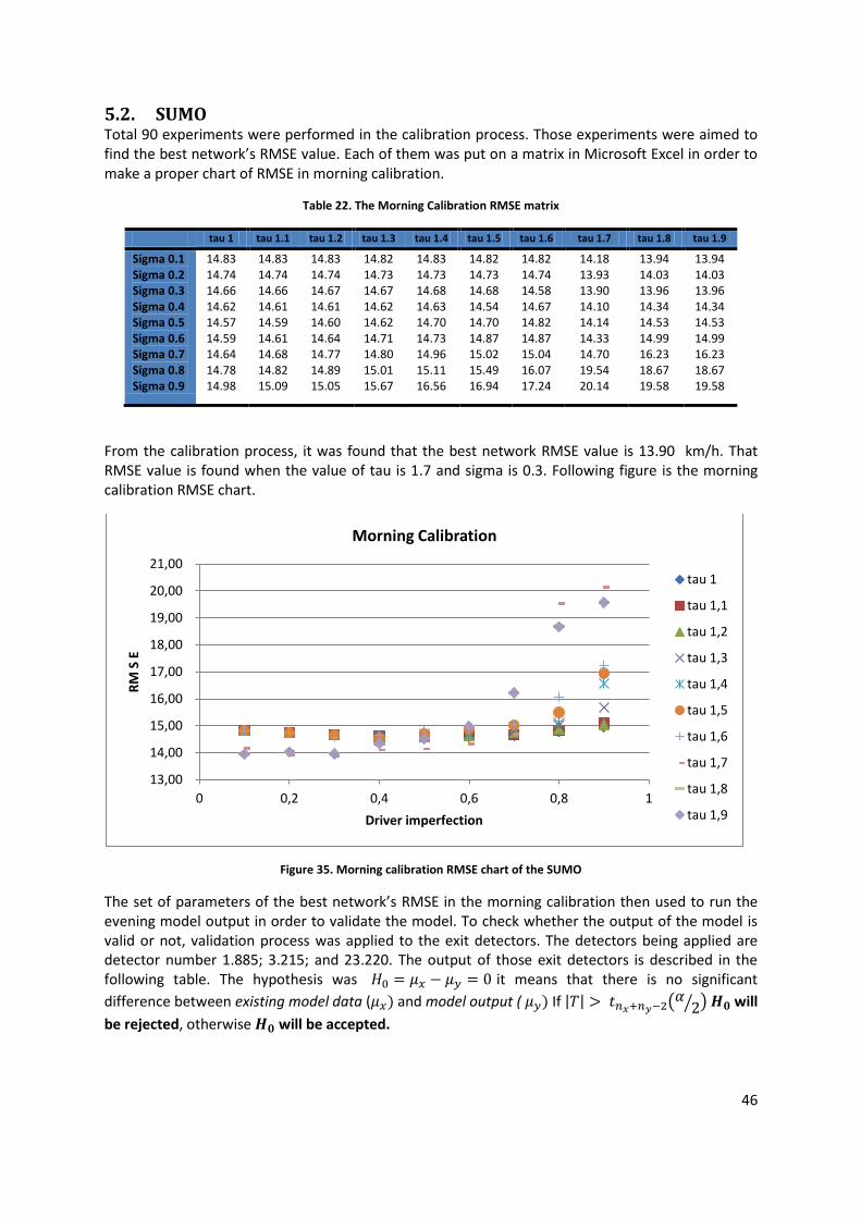
46

5.2. SUMO Total 90 experiments were performed in the calibration process. Those experiments were aimed to find the best network’s RMSE value. Each of them was put on a matrix in Microsoft Excel in order to make a proper chart of RMSE in morning calibration.

Table 22. The Morning Calibration RMSE matrix

tau 1 tau 1.1 tau 1.2 tau 1.3 tau 1.4 tau 1.5 tau 1.6 tau 1.7 tau 1.8 tau 1.9

Sigma 0.1 Sigma 0.2 Sigma 0.3 Sigma 0.4 Sigma 0.5 Sigma 0.6 Sigma 0.7 Sigma 0.8 Sigma 0.9

14.83 14.74 14.66 14.62 14.57 14.59 14.64 14.78 14.98

14.83 14.74 14.66 14.61 14.59 14.61 14.68 14.82 15.09

14.83 14.74 14.67 14.61 14.60 14.64 14.77 14.89 15.05

14.82 14.73 14.67 14.62 14.62 14.71 14.80 15.01 15.67

14.83 14.73 14.68 14.63 14.70 14.73 14.96 15.11 16.56

14.82 14.73 14.68 14.54 14.70 14.87 15.02 15.49 16.94

14.82 14.74 14.58 14.67 14.82 14.87 15.04 16.07 17.24

14.18 13.93 13.90 14.10 14.14 14.33 14.70 19.54 20.14

13.94 14.03 13.96 14.34 14.53 14.99 16.23 18.67 19.58

13.94 14.03 13.96 14.34 14.53 14.99 16.23 18.67 19.58

From the calibration process, it was found that the best network RMSE value is 13.90 km/h. That RMSE value is found when the value of tau is 1.7 and sigma is 0.3. Following figure is the morning calibration RMSE chart.

Figure 35. Morning calibration RMSE chart of the SUMO

The set of parameters of the best network’s RMSE in the morning calibration then used to run the evening model output in order to validate the model. To check whether the output of the model is valid or not, validation process was applied to the exit detectors. The detectors being applied are detector number 1.885; 3.215; and 23.220. The output of those exit detectors is described in the following table. The hypothesis was it means that there is no significant

difference between existing model data ( and model output ( If

will

be rejected, otherwise will be accepted.

13,00

14,00

15,00

16,00

17,00

18,00

19,00

20,00

21,00

0 0,2 0,4 0,6 0,8 1

RM

S E

Driver imperfection

Morning Calibration

tau 1

tau 1,1

tau 1,2

tau 1,3

tau 1,4

tau 1,5

tau 1,6

tau 1,7

tau 1,8

tau 1,9

47

Table 23. t-Test Validation against speed data

1.885 23.220 3.215

Sp2 1.96 0.11 0.67

T (1.98) (3.06) (16.15)

T 2.01 2.01 2.01

Accept Ho Reject Ho Reject Ho

Table 24. t-Test Validation against flow data

1.885 23.220 3.215

Sp2 420.604 228.343 458.55

T -24.555 10.65 -11.674

T 2.013 2.013 2.013

Reject Ho Reject Ho Reject Ho

As seen in table 23 above, two of three detectors are resulting rejected values. On the contrary, table 24 shows us that the flow validation is resulting none of them has accepted values. Rejected value means that |T| or T-count < T-table or t. Based on validation of flow data of the SUMO, the model cannot be used for those three detectors. The chart of validation result can be seen in the following figures.

In figure 37 below, we can see that there is a big gap between observation and the model output chart. The gap exists due to there were several collisions occurred in one of junctions on the northern side of Södra länken Tunnel. The collisions not only made the traffic’s speed around that road decreasing but also affecting the amount of flow passing through it.

Though SUMO is a micro-simulation software using the collision –free model, collisions are still occurred. For this simulation, the collisions occurred in junction no 1445695315(figure 36) where it is a narrowed junction from three lanes to two lanes on the northern side of Södra Länken Tunnel. The collisions were happen when cars from the 2nd and the 1st lane are joining to the first lane on the next edge while cars from the 3rd lane are continuing their travel to the second lane on the next edge. This problem cannot be solved by only shifting the traffic from 2nd lane to join with the 3rd lane to second lane on the next edge, because it just shifting the collisions from the 1st lane to the 2nd lane of the next edge.

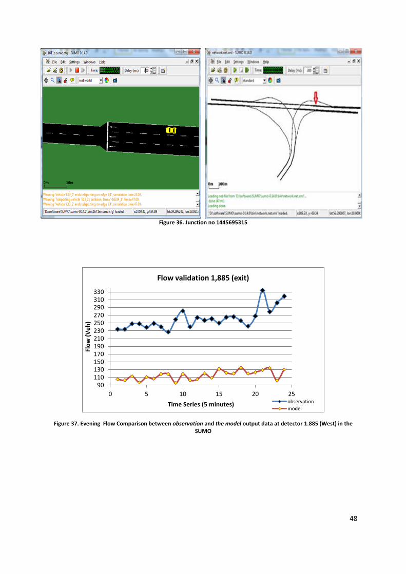
48

Figure 36. Junction no 1445695315

Figure 37. Evening Flow Comparison between observation and the model output data at detector 1.885 (West) in the SUMO

90 110 130 150 170 190 210 230 250 270 290 310 330

0 5 10 15 20 25

Flo

w (

Ve

h)

Time Series (5 minutes)

Flow validation 1,885 (exit)

observation

model

49

Figure 38. Evening Flow Comparison between observation and the model output data at detector 23.220 (South) in the SUMO

Figure 39. Evening Flow Comparison between observation and the model output data at detector 3.215 (South) in the SUMO

Instead of continuing the validation process until all the detectors resulting significant or accepted result, this research was ending up the validation. The reason of why it was stopping the validation process is because the purpose of this thesis is to compare micro-simulation software used in this thesis.

Detector 1.885 has three series of detector in it such as detector no 49, 50 and 51. Detector no 49 is the slowest lane or the most right lane and so on. In figure 40 below, the speed is started at low mean speed value for the first 5 minutes. Afterwards it happens again in the 23th set of 5 minute. Those conditions happened because of there was no vehicles passing through detector 51 of detector number 1.885 on those intervals. The absences of vehicles passing through one of the detector on those intervals made the mean speed chart above shows drastic changes.

50

60

70

80

90

100

110

120

130

140

150

160

0 5 10 15 20 25

Flo

w

Time Series (5 minutes)

Flow validation 23,220 (exit)

observation model

170

190

210

230

250

270

290

310

330

0 5 10 15 20 25

Flo

w

Time Series (5 minutes)

Flow validation 3,215 (exit)

observation

model

50

Figure 40. Evening Speed Comparison between observation and the model output data at detector 1.885 (West) in the SUMO

Figure 41. Evening Speed Comparison between observation and the model output data at detector 23.220 (South) in the SUMO

For the speed validation result, peculiarity occurred. In figure 42, we can see that in the detector number 3.215 at the model chart speed is increasing in last interval. Beforehand, detector 3.215 has 4 set of detectors and the line expressed on the chart is derived from the average speed of those detectors. From the 1st interval to 23rd, only 3 detectors were passed by the vehicles. However, when it came to the 24th interval, all detectors were passed by vehicles. This is the reason why in the last interval of detector 3.215 the model speed suddenly increase.

40

45

50

55

60

65

70

75

1 6 11 16 21

Me

an s

pe

ed

(km

/h)

Time series (5 minutes)

Speed validation 1,885 (exit)

observation

model

64

66

68

70

72

1 5 9 13 17 21

Me

an s

pe

ed

(km

/h)

Time series (5 minutes)

Speed validation 23,220 (exit)

observation

model

51

Figure 42. Evening Speed Comparison between observation and the model output data at detector 3.215 (East) in the SUMO

5.3. COMPARISON AIMSUN AND SUMO 5.3.1. Result on Speed and Flow According to the result from both software, it can be seen that for speed and flow AIMSUN gave closer result to the observation data than SUMO did. Figure 43 shows comparison graphic of flow on three exit points/detectors. This comparison used evening observation flow data compare to the flow resulted from the two softwares SUMO and AIMSUN using evening traffic demand.

Figure 43. Comparison between SUMO and AIMSUN in Evening flow data on exit detectors

45

50

55

60

65

70

1 6 11 16 21

Me

an s

pe

ed

(km

/h)

Time series (5 minutes)

Speed validation 3,215 (exit)

observation model

40

60

80

100

120

140

160

0 5 10 15 20 25

Flo

w (

Ve

h)

Time Series (5 minutes)

23,220 (exit) South

observation SUMOAIMSUN

150

170

190

210

230

250

270

290

310

330

350

0 5 10 15 20 25

Flo

w (

ve

h)

Time Series (5 minutes)

3,215 (exit) East

observation SUMOAIMSUN

50

100

150

200

250

300

350

0 5 10 15 20 25

Flo

w (

Ve

h)

Time series (5 minutes)

1,885 (exit) West

observation SUMOAIMSUN

52

When comparison is made using evening speed data from the two softwares SUMO and AIMSUN, there are differences in the result. On detector 23.220 and 1.885 SUMO give better result than AIMSUN. In figure 44 it can be seen that in both detectors the result form SUMO are closer than AIMSUN to the observation data.

Even though in comparison using speed data SUMO give better result in two exit detectors, AIMSUN still better software since in comparison using flow data AIMSUN give better result in all exit detectors. For flow data, AIMSUN still gives the better result than SUMO. At least there are three reasons causing this fact. The first reason is due to the infrastructure accuracy level of AIMSUN is better than SUMO. For example, AIMSUN can build kerb on it while in the SUMO can’t. The second reason is because of the fact that in the SUMO model occurred several collisions which made the flow became small. The last reason is due to not all vehicles in the model were passing through each detectors set in every time intervals.

Figure 44. Comparison between SUMO and AIMSUN in Evening speed data on exit detectors

Table 25. Comparison of validation on SUMO and AIMSUN by using evening flow data

Detector t Stat AIMSUN

t Stat SUMO

t Critical two-tail

Classification

AIMSUN SUMO

23.220 (South) 1.323 10.65 2.018 Accept Ho Reject Ho

1.885 (West) 5.523 -24.55 2.018 Reject Ho Reject Ho

3.215 (East) -0.713 -11.67 2.018 Accept Ho Reject Ho

55

57

59

61

63

65

67

69

71

73

75

0 5 10 15 20 25

Sp

ee

d (

km

/h

)

Time Series (5 minutes)

23,220 (exit) South

observation SUMOAIMSUN

40

45

50

55

60

65

70

75

0 5 10 15 20 25

Sp

ee

d (

km

/h

)

Time Series (5 minutes)

1,885 (exit) West

observation SUMOAIMSUN

50

55

60

65

70

75

0 5 10 15 20 25

Sp

ee

d (

km

/h

)

Time Series (5 minutes)

3,215 (exit) East

observation SUMOAIMSUN

53

On table 25 shows that by using evening flow data for validation the model from both software AIMSUN and SUMO, AIMSUN give better result. Even though figure 42 shows that SUMO give closer speed to the observation speed data, but in table 26 it can be seen that statistically SUMO did not give better result than AIMSUN.

Table 26. Comparison of validation on SUMO and AIMSUN by using evening speed data

Detector t Stat AIMSUN

t Stat SUMO

t Critical two-tail

Classification

AIMSUN SUMO

23.220 (South) 15.33 -3.06 2.018 Reject Ho Reject Ho

1.885 (West) 4.37 -1.98 2.018 Reject Ho Accept Ho

3.215 (East) -0.69 -16.15 2.018 Accept Ho Reject Ho

5.3.2. Network AIMSUN gives much saving time for user to develop the network rather than SUMO. User interface in AIMSUN make user possible to directly draw the network when operating the software, in the other side SUMO has complicated system for network building. In the SUMO user have to declare the network attributes for all infrastructure. SUMO’s user has to create kind of coding system in XML files to make it sure that the network connected, while AIMSUN facilitate user the option for creating, editing, adding the network.

AIMSUN and SUMO have similarities in order to make their user less difficult in network building. Both of them have option that can make their user importing network file from other software. For SUMO, the network can be imported from OpenStreetMap; VISUM; Vissim; openDRIVE, MATsim; ArcView; Elmar’s; Robocup; Simulation League (20). There should be some adjustments before it can be use or displayed in the SUMO-GUI. However, the imported network should also compared to the network map owned by the authorities i.e. FHWA, Trafikverket, etc. in order to have a good and exact picture of the network. AIMSUN network can be imported from Getram; GIS(Shapefiles); Image File; 3D Studio; Wavefront; DWG/DXF; AutoCAD Drawing File; EMME/2; CONTRAM Network; SATURN Network; Paramics Network; Synchro Control Plan (21).

5.3.3. Demand AIMSUN and SUMO have similarity in demand modification for the model input. Both of this software using O/D matrix as demand input data for develop their model. The different is on the easiness to access the option to O/D Matrix modification. AIMSUN gives access for user to directly modify the O/D Matrix. The modified O/D Matrix then will automatically compile in “traffic demand” file as mentioned in previous part. On SUMO, user has to modify XML file to modify the demand (flow) for each lane or direction. The modification has to be performed in each lane for each time interval.

Demand modification of the SUMO is very vulnerable for error or mistaken because demand data should be modified on its XML file. When the user wants to change the number of demand, they have to change it lane by lane for each direction and for each time interval. For this kind of problem, AIMSUN make it easier by giving the user chance to decrease or increase the demand just by put percentage in each O/D matrix.

5.3.4. Control SUMO has three different files to perform a simulation, one of those file is configuration file that control about network and demand file that will be run on each simulation. In GUI of SUMO, user has to determine or call the configuration file and network before perform the simulation. Every

54

time a modification occurred, SUMO users should make an adjustment. The adjustment can be saved the file, using duarouter application to combine the network, car following and flow data so that the configuration file can recognize the new modification. This step will consume more memory in PC, but this problem can be measured by transfer the output file in XLM format into excel file after each experiment. SUMO processing an experiment within less time since this software does not need high specification of a PC.

AIMSUN have more simple steps for control each experiment. User just needs to determine about behavioral parameter in each experiment. There is no configuration file in AIMSUN for each experiment. User just needs to make sure that value of parameter in each experiment is on the right value. AIMSUN simulation processing consume more time for each experiment, greater the number of replication in each experiment the longer time needed for AIMSUN to process an experiment.

5.3.5. Output AIMSUN and SUMO have different system for output storage. SUMO software generate output file in XML extension which have size 150-200 kB for each experiment output file. The size of files will be larger depends on the network size. XML file from SUMO can be opened on Excel to ease the calculation. In the other side, AIMSUN generates more file size as output file for each experiment performed. Each replication in each experiment has unique number which will be recognized when the user want to find exact data. The output file can be opened using Microsoft Access Database and based on experience in this research the output file size can be up to 500 MB for 15 experiments with 10 replications in each experiment. Output in AIMSUN contains information about performance of the network. Time interval produced in output file is determined by the user when define the scenario.

5.3.6. Guidance AIMSUN provide guidance for their user by User’s Manual on its software. As open source software, SUMO is also providing the guidance for all its users. The user manual can be downloaded from SUMO’s website. The website also contains the guidance about how to build the network and all things needed in the SUMO, including short tutorial. This tutorial was really helpful for user to understanding SUMO. Although do not give any tutorial in the guidance, AIMSUN provide detailed information about software on AIMSUN User Manual which can directly accessed while working on the software. AIMSUN user does not need to open internet browser to find guidance related to the software.

5.3.7. Technical support In the term of graphical interface, AIMSUN provide more advantages to the user by giving option for 2D or 3D display with higher detail of animation than SUMO which just can perform 2D animation display. High detail of animation in AIMSUN needs high-end specification of PC as consequences such as 2GB RAM or 200 MB hard-disk capacity should be provided in PC. SUMO software is really easy to be installed since it comes with small size of software. SUMO platform is compliable using most platforms (22)

55

Table 27. Comparison AIMSUN and SUMO

NO AIMSUN SUMO

1 Model Development

Network Directly created in the software operation through GUI

Have option to import the network from other software

Created in XML file by defining each link and each connection/intersection

Have option to import the network from other software but still have to be converted

Traffic Demand O/D matrix for each time interval

Turning proportion

Manually defined in XML file along with link coding for each time interval

Run Control Need to check the value of parameter for each experiment.

An experiment can contains several replication

Checking XML file of Network, Demand and configuration in each experiment.

Output .dbf file which can be opened by using Microsoft Access Database

.XML file which can be opened by Microsoft Office Excel

2 Technical Aspect

Computer Specification Middle to high end specification

Compatible for windows, Mac OS X and Linux

Low to middle end specification

Compatible in almost all platform

Animation Display 2D 3D Smooth animation

2D Low detail animation

User Skill User friendly for non-programming user

Programming skill is recommended

License Limited Free (Open-Source)

Improvement Rare Relatively often User can fully involved in

improvement Guidance Directly accessed from “Help”

option in the software Internet browser needed

56

CHAPTER 6 CONCLUSIONS

Based on the comparison of the results of the two softwares for the studied area, it can be concluded that AIMSUN model performes better than the SUMO model. Regarding the complexity aspect of using the softwares, SUMO is more complex system to get used to than AIMSUN. For the user, AIMSUN provide easiness by its GUI (Graphical User Interface) for building network, demand and control for each experiment.

The SUMO software outputs speed data in the unit of m/s and AIMSUN outputs speed data in km/h unit. This condition affected the value of RMSE. In order to compare the software, the speed from SUMO is converted into km/h. After converting the speed, SUMO resulted in a RMSE value which is 13.90 lower than the value for AIMSUN. Based on the value of RMSE, SUMO gave better results. But it should be noted that AIMSUN calculate the average of its 10-replications while SUMO only calculate one replication. Each replication in AIMSUN gives different model output, several replications give higher model output than observed data and other replications give lower model output than observed data. When the calibrated-model from the two softwares was applied to the evening demand, AIMSUN result in a better validation than SUMO. The calibrated Sumo model gave result that significantly different from the observed data at all detectors while the calibrated AIMSUN model gave result not significantly different from the observation data on most detectors.

In this thesis, two simulation models have been constructed, one for AIMSUN and one for SUMO. The AIMSUN model is calibrated using theparameters “Speed Acceptance” and “Maximum Desired Speed”. The best set of parameters based on RMSE value is on 1.1 for Speed Acceptance and 100 km/h for Maximum Desired Speed with RMSE value at this level is 19.394. However, when this set of parameter was validated against evening-flow data it turns out that the model is not statistically valid for all detectors. The detector 1.885, in the west section, is the detector that is not valid against evening-flow data. The SUMO model was calibrated using the parameters Driver ImperfectionDriver’s Reaction Time. It was found that the best set of parameters based on its RMSE value is when 0.3 and 1.7, respectively, with a RMSE value of 13.90. When the validation process of the SUMO was performed against evening-speed data, similar conclusions as for the AIMSUN model can be drawn. The result of validation shows that the model is not valid for all detectors. Validation result shows that the model output data on detector 1.885 is significantly different with observation data.

The calibration process in this thesis was limited to adjusts two parameters. More parameters can be adjusted in the calibration process in order to get better results.

In a feature comparison, the AIMSUN and SUMO softwares are relatively similar. AIMSUN, as a commercial micro-simulation software, has more options when building the network. Whereas in SUMO user has to write an XML file to create detectors. This step is very vulnerable for user mistakes. These features of SUMO make it more suitable for academic purposes and the software requires a more deep understanding about the software and micro-simulation in general. The AIMSUN 6.1 version in this research has many advantages. A user can relatively easily build, draw or import the network, setting the parameters, and run the model. A user’s manual is available. The software reuqires a license The software also require a relatively high specification of the PC to handle the simulation and animations. There is no option for user to apply different behavior parameter like lane-changing or the car-following model in different areas within a network.

SUMO 0.14.0 which was used for this thesis is accessible for everyone through the website. The complexity of the software can stimulate the user to more carefully build the model. The

57

complexities also give good basic experience for user in micro-simulation model building. The Free license of this software makes it easy for everyone to use it or maybe give contribution in its improvement. The complexities of SUMO software obviously give several drawbacks. It will be vulnerable for user to make mistakes in network or demand coding in the XML files. A user also will have have to spend significant time for creating infrastructure feature such as detectors, pedestrian crossings, and other infrastructure features.

58

REFERENCES

1. Transport Simulation System. AIMSUN. [Online].; 2010 [cited 2012 February. Available from:

http://www.aimsun.com/wp/?page_id=21.

2. google. maps.google.com. [Online]. [cited 2012 04 15. Available from: http://maps.google.com/.

3. OpenStreetMap. OpenStreetMap. [Online].; 2012 [cited 2012 04. Available from:

http://www.openstreetmap.org/.

4. Drew DR. Traffic Flow Theory and Control New York: McGraw-Hill; 1968.

5. Kallberg H. Traffic Simulation (in Finnish): Helsinki University of Technology, Transportation

Engineering. Espoo; 1971.

6. Alexiadis V, Jeannotte K, Chandra A. Traffic Analysis Toolbox Volume I: Traffic Analysis Tools

Primer Oackland, CA: US. Department of Transportation; 2004.

7. Olstam JJ. A Model for Simulation and Generation of Surrounding Vehicles in Driving Simulators

Norrkoping: UniTryck; 2005.

8. TSS-Transport Simulation Systems. Microsimulator and Mesosimulator Aimsun 6.1 User's

Manual: TSS-Transport Simulation Systems. S.L.; 2010.

9. German Aerospace Center, Instute of Transportation Systems. sourceforge.net. [Online].; 2011

[cited 2012 February 16. Available from:

http://sumo.sourceforge.net/doc/current/docs/userdoc/SUMO_User_Documentation.html.

10. Behrisch M, Bieker L, Erdmann J, Krajzewicz D. SUMO - Simulation of Urban Mobility, An

Overview. In The Third International Conference on Advances in System Simulation; 2011; Berlin:

Institute of Transportation Systems, German Aerospace Center. p. 1.

11. Krajzewicz D, Behrisch M. SUMO - Simulation of Urban MObility - User Documentation.

12. Dowling R, Skabardonis A, Alexiadis V. Traffic Analysis Toolbox Volume III: Guidelines for applying

Traffic Microsimulation Software Washington D.C: U.S. Department of Transportation; 2004.

13. Holmes S. RMS Error. [Online].; 2000 [cited 2012 June 21. Available from: http://www-

stat.stanford.edu/~susan/courses/s60/split/node60.html.

14. Behrisch M, Bieker L, Erdmann J, Krajzweicz D. SUMO - Simulation of Urban MObility An

Overview. Berilin, Germany: Institute of Transportation Systems German Aerospace Center;

2011. Report No.: ISBN: 978-1-61208-169-4.

59

15. Bieker L. Emergency Vehicle prioritization using Vehicle to-Infrastructure Communication. In

Young Researchers Seminar 2011 (YRS2011); 2011; Vienna, Austria.

16. Bieker L, Krajzewicz D. Evaluation of opening Bus Lanes for private Traffic triggered via V2X

Communication; 2011.

17. Olstam JJ, Tapani A. Comparison of Car-following models. Sweden: Swedish National Road and

Transport Research Institute; 2004.

18. TSS-Transport Simulation System. Aimsun 6.1 User's Manual. June 2010..

19. Krausszlig S. sourceforge.net. [Online].; 1998 [cited 2012 April 19. Available from:

http://sumo.sourceforge.net/pdf/KraussDiss.pdf.

20. German Aerospace Center. sumo.sourceforge.net. [Online].; 2011 [cited 2012 05. Available from:

http://sumo.sourceforge.net/doc/current/docs/userdoc/Networks/SUMO_Road_Networks.html

.

21. TSS-Transport Simulation System. Aimsun 6.1 Users Manual TSS-Transport Simulation Systems

SL, editor.: TSS-Transport Simulation Systems, S.L; 2010.

22. Krajzewicz D, Hertkorn G, Wagner P. SUMO (Simulation of Urban MObility) An open-source

traffic simulation. Berlin: German Aerospace Centre.

23. Lansdowne A. Traffic Simulation using Agent-Based Modelling England: University of the West of

England; 2006.

24. System IoT. SUMO - Simulation of Urban MObility. [Online].; 2012 [cited 2012 April 19. Available

from: http://sumo.sourceforge.net/doc/current/docs/userdoc/index.html.

25. Fox K. Introduction to Micro-simulation. [Online]. [cited 2012 January 9. Available from:

http://www.microsimulation.drfox.org.uk/intro.html.

26. Barceló J, Ferrer J, García D, Grau R, Forian M, Chabini I, et al. Microscopic Traffic Simulation for

ATT Systems Analysis A Parallel Computing Version France: Centre de Recherche sur les

Transports; 1998.

27. Krauss S. Microscopic Modeling of Traffic Flow: Investigation of Collision Free Vehicle Dynamics

Koln: Universitat zu Koln; 1998.

a

APPENDIXES

A. SUPPLIED DEMAND DATA

1) Morning Demand (entrance Detectors)

Time Detector

2,305 1,845 3,270

Flow Speed Flow Speed Flow Speed

6:30:00 - 6:35:00 130 67,36 320 72,94 314 65,25

6:36:00 - 6:40:00 153 64,4 255 73,53 296 67,5

6:41:00 - 6:45:00 156 64,1 291 71,93 293 56,65

6:46:00 - 6:50:00 172 61 300 73,60 292 37,3

6:51:00 - 6:55:00 162 64,3 262 73,53 291 36

6:56:00 - 7:00:00 170 63,3 261 72,33 292 36,9

7:01:00 - 6:05:00 175 62,4 267 70,33 309 37,7

7:06:00 - 7:10:00 152 60,4 239 72,13 252 33,05

7:11:00 - 7:15:00 139 61,7 240 71,47 212 27,55

7:16:00 - 7:20:00 174 60,7 254 70,67 198 29,1

7:21:00 - 7:25:00 166 59,6 257 70,40 199 29,65

7:26:00 - 7:30:00 143 60,4 269 67,80 249 28,7

7:31:00 - 7:35:00 139 64,3 272 69,47 212 28,65

7:36:00 - 7:40:00 170 61 262 71,13 213 30,9

7:41:00 - 7:45:00 138 62,9 275 70,67 175 25,35

7:46:00 - 7:50:00 152 61,3 287 67,73 167 28,1

7:51:00 - 7:55:00 142 61,9 242 71,67 261 28,15

7:56:00 - 8:00:00 160 60,6 247 70,13 180 25,65

8:01:00 - 8:05:00 152 60,3 243 71,93 168 29,45

8:06:00 - 8:10:00 152 61,7 222 50,40 165 37,2

8:11:00 - 8:15:00 149 61,5 147 20,60 240 30,7

8:16:00 - 8:20:00 137 63,5 144 20,40 133 23,15

8:21:00 - 8:25:00 141 62,9 135 18,33 214 31,25

8:26:00 - 8:30:00 119 63,4 124 18,80 173 29,9

3643 5815 5498

b

2) Morning Demand (Exit Detectors)

Time Detector

2300e 23,495 3,015h 23,49

Flow Speed Flow Speed Flow Speed Flow Speed

6:30:00 - 6:35:00 11 72,00 76 67,5 51 76,33 65 68,2

6:36:00 - 6:40:00 9 66,00 72 67,8 40 76,6 90 65,8

6:41:00 - 6:45:00 11 70,00 71 66,2 48 73,4 77 66

6:46:00 - 6:50:00 4 73,00 98 63,6 63 73,2 76 66,2

6:51:00 - 6:55:00 14 74,00 93 64 52 71,2 84 64,4

6:56:00 - 7:00:00 25 71,00 98 63,2 57 72,6 68 67,2

7:01:00 - 6:05:00 23 68,50 93 65,2 56 73,4 81 64,4

7:06:00 - 7:10:00 11 74,00 83 65,4 66 69,2 75 64,2

7:11:00 - 7:15:00 11 70,00 74 62,2 65 63,4 70 61,6

7:16:00 - 7:20:00 8 73,00 88 63 62 68,8 81 63

7:21:00 - 7:25:00 0 0,00 73 64,6 67 67,6 91 60,4

7:26:00 - 7:30:00 0 0,00 91 62,6 67 65,4 75 62,2

7:31:00 - 7:35:00 22 67,33 71 68,4 63 62,2 70 66

7:36:00 - 7:40:00 11 75,00 88 60,2 65 66,2 78 63,8

7:41:00 - 7:45:00 14 69,50 75 65,4 66 62,2 73 63,8

7:46:00 - 7:50:00 5 68,00 90 63 69 63,8 67 64,2

7:51:00 - 7:55:00 4 74,00 69 64,6 63 64,2 77 63

7:56:00 - 8:00:00 15 69,00 64 64,2 60 63 92 61,8

8:01:00 - 8:05:00 7 74,50 95 60 54 66,2 71 62,2

8:06:00 - 8:10:00 12 62,00 81 63 59 61,8 72 63,8

8:11:00 - 8:15:00 10 59,50 81 62,4 58 65,8 66 62,8

8:16:00 - 8:20:00 23 58,25 65 63,4 55 63,4 81 62,4

8:21:00 - 8:25:00 17 63,50 71 63,4 52 67 74 60,2

8:26:00 - 8:30:00 8 62,50 64 64,2 44 66 59 63,4

Total 275 1924 1402 1813

c

3) Matrix of Morning Demand (5 minutes interval)

1 West East South 7 West East South

West 0 309 11 West 0 244 23

East 263 0 51 East 253 0 56

South 54 76 0 South 82 93 0

2 West East South 8 West East South

West 0 246 9 West 0 228 11

East 256 0 40 East 186 0 66

South 81 72 0 South 69 83 0

3 West East South 9 West East South

West 0 280 11 West 0 229 11

East 245 0 48 East 147 0 65

South 85 71 0 South 65 74 0

4 West East South 10 West East South

West 0 296 4 West 0 246 8

East 229 0 63 East 136 0 62

South 74 98 0 South 86 88 0

5 West East South 11 West East South

West 0 248 14 West 0 257 0

East 239 0 52 East 132 0 67

South 69 93 0 South 93 73 0

6 West East South 12 West East South

West 0 236 25 West 0 269 0

East 235 0 57 East 182 0 67

South 72 98 0 South 52 91 0

d

Matrix of Morning Demand (5 minutes interval)

13 West East South 19 West East South

West 0 250 22 West 0 236 7

East 149 0 63 East 114 0 54

South 68 71 0 South 57 95 0

14 West East South 20 West East South

West 0 251 11 West 0 210 12

East 148 0 65 East 106 0 59

South 82 88 0 South 71 81 0

15 West East South 21 West East South

West 0 261 14 West 0 137 10

East 109 0 66 East 182 0 58

South 63 75 0 South 68 81 0

16 West East South 22 West East South

West 0 282 5 West 0 121 23

East 98 0 69 East 78 0 55

South 62 90 0 South 72 65 0

17 West East South 23 West East South

West 0 238 4 West 0 118 17

East 198 0 63 East 162 0 52

South 73 69 0 South 70 71 0

18 West East South 24 West East South

West 0 232 15 West 0 116 8

East 120 0 60 East 129 0 44

South 96 64 0 South 55 64 0

e

4) Evening Demand (entrance Detectors)

Time Detector

2,305 1,845 3,27

Flow Speed Flow Speed Flow Speed

13:30:00 - 13:35:00 74 64,5 311 68,22 260 67,5

13:36:00 - 13:40:00 69 64 235 70,53 230 69,65

13:41:00 - 13:45:00 71 63,1 259 67,53 243 67,8

13:46:00 - 13:50:00 75 66,2 245 69,40 236 68

13:51:00 - 13:55:00 98 64,3 243 68,47 228 76,7

13:56:00 - 14:00:00 84 65,6 250 69,07 235 76,45

14:01:00 - 14:05:00 78 65,1 228 70,93 229 68,05

14:06:00 - 14:10:00 71 65,7 247 68,07 231 67,6

14:11:00 - 14:15:00 85 65 268 68,80 257 76

14:16:00 - 14:20:00 99 64 249 71,60 253 77,15

14:21:00 - 14:25:00 87 65,1 243 70,40 237 67,55

14:26:00 - 14:30:00 85 65,3 258 69,13 248 68,45

14:31:00 - 14:35:00 74 65,3 260 68,53 241 67,4

14:36:00 - 14:40:00 105 64,3 254 69,20 240 65,95

14:41:00 - 14:45:00 88 62,5 260 67,67 277 67,45

14:46:00 - 14:50:00 110 62 248 68,73 224 77,65

14:51:00 - 14:55:00 88 66 297 66,27 231 69,5

14:56:00 - 15:00:00 63 84,6 279 62,67 254 67,7

15:01:00 - 15:05:00 96 66,9 313 64,27 306 64,5

15:06:00 - 15:10:00 119 65,2 304 57,87 285 65,8

15:11:00 - 15:15:00 100 62,7 311 42,53 264 67,4

15:16:00 - 15:20:00 90 63,8 292 34,13 286 65,2

15:21:00 - 15:25:00 109 65 291 36,60 306 65,05

2018 6210 5801

f

5) Evening Demand (Exit Detectors)

Time Detector

2300e 23,495 3,015 23,49

Flow Speed Flow Speed Flow Speed Flow Speed

13:30:00 - 13:35:00 25 66,20 47 66 49 71,2 38 71,16

13:36:00 - 13:40:00 25 69,25 45 65,6 44 72,4 30 67,6

13:41:00 - 13:45:00 28 66,50 44 65,4 66 71,4 39 69,8

13:46:00 - 13:50:00 10 68,50 45 67,8 53 71,8 31 69,6

13:51:00 - 13:55:00 13 70,50 53 65 60 71,4 44 67,4

13:56:00 - 14:00:00 7 66,00 50 66,8 53 73,4 33 70

14:01:00 - 14:05:00 12 66,00 53 66 44 75,8 25 68,2

14:06:00 - 14:10:00 11 68,00 40 65,2 42 76,2 36 68,2

14:11:00 - 14:15:00 23 72,33 61 64,4 63 72 23 67,8

14:16:00 - 14:20:00 18 70,33 51 65 63 74,2 48 65,8

14:21:00 - 14:25:00 28 70,25 53 66 57 72,8 36 69,4

14:26:00 - 14:30:00 30 68,00 61 64,6 65 75 28 68,6

14:31:00 - 14:35:00 12 66,50 36 67 50 73,4 44 69,2

14:36:00 - 14:40:00 20 71,25 56 64,2 62 69,6 46 67,4

14:41:00 - 14:45:00 23 68,00 54 64,2 66 73,6 39 66,6

14:46:00 - 14:50:00 19 69,67 60 63 54 72 47 66,4

14:51:00 - 14:55:00 35 69,25 36 69,8 60 71,8 38 66,8

14:56:00 - 15:00:00 29 70,00 49 64,6 62 70,8 26 69

15:01:00 - 15:05:00 18 69,50 48 67 63 71,4 44 71,2

15:06:00 - 15:10:00 31 68,25 63 63,6 67 74 61 67,6

15:11:00 - 15:15:00 59 63,50 69 63,8 61 75,6 36 69

15:16:00 - 15:20:00 23 69,00 49 66,6 57 71,2 41 68,6

15:21:00 - 15:25:00 46 63,25 71 63,2 66 72,2 34 67,4

Total 545 1194 1327 867

g

6) Matrix of Evening Demand (5 minutes interval)

1 West East South 7 West East South

West 0 286 25 West 0 216 12

East 211 0 49 East 185 0 44

South 27 47 0 South 25 53 0

2 West East South 8 West East South

West 0 210 25 West 0 236 11

East 186 0 44 East 189 0 42

South 24 45 0 South 31 40 0

3 West East South 9 West East South

West 0 231 28 West 0 245 23

East 177 0 66 East 194 0 63

South 27 44 0 South 24 61 0

4 West East South 10 West East South

West 0 235 10 West 0 231 18

East 183 0 53 East 190 0 63

South 30 45 0 South 48 51 0

5 West East South 11 West East South

West 0 230 13 West 0 215 28

East 168 0 60 East 180 0 57

South 45 53 0 South 34 53 0

6 West East South 12 West East South

West 0 243 7 West 0 228 30

East 182 0 53 East 183 0 65

South 34 50 0 South 24 61 0

h

Matrix of Evening Demand (5 minutes interval)

13 West East South 19 West East South

West 0 248 12 West 0 295 18

East 191 0 50 East 243 0 63

South 38 36 0 South 48 48 0

14 West East South 20 West East South

West 0 234 20 West 0 273 31

East 178 0 62 East 218 0 67

South 49 56 0 South 56 63 0

15 West East South 21 West East South

West 0 237 23 West 0 252 59

East 211 0 66 East 203 0 61

South 34 54 0 South 31 69 0

16 West East South 22 West East South

West 0 229 19 West 0 269 23

East 170 0 54 East 229 0 57

South 50 60 0 South 41 49 0

17 West East South 23 West East South

West 0 262 35 West 0 245 46

East 171 0 60 East 240 0 66

South 52 36 0 South 38 71 0

18 West East South 24 West East South

West 0 250 29 West 0 65 0

East 192 0 62 East 0 0 0

South 14 49 0 South 0 0 0

i

B. AIMSUN CALIBRATION

1) Calibration Process Entrance Detectors

Time Detector

23,205 13920 (Model)

1,845

26431 (Model)

3,270

26432 (Model)

Speed speed Speed speed Speed speed

6:30:00 - 6:35:00 67,36 6,28 64,86 72,94 112,70 62,33 65,25 0,59 66,02

6:36:00 - 6:40:00 64,4 13,59 60,71 73,53 121,53 62,51 67,50 12,18 64,01

6:41:00 - 6:45:00 64,1 15,31 60,19 71,93 133,00 60,40 56,65 60,67 64,44

6:46:00 - 6:50:00 61 13,03 57,39 73,60 184,98 60,00 37,30 759,27 64,85

6:51:00 - 6:55:00 64,3 60,40 56,53 73,53 160,73 60,86 36,00 844,97 65,07

6:56:00 - 7:00:00 63,3 54,46 55,92 72,33 101,04 62,28 36,90 775,81 64,75

7:01:00 - 6:05:00 62,4 41,73 55,94 70,33 66,52 62,18 37,70 742,63 64,95

7:06:00 - 7:10:00 60,4 1,14 59,33 72,13 52,33 64,90 33,05 1072,16 65,79

7:11:00 - 7:15:00 61,7 0,85 60,78 71,47 58,94 63,79 27,55 1564,33 67,10

7:16:00 - 7:20:00 60,7 51,22 53,54 70,67 49,33 63,64 29,10 1570,80 68,73

7:21:00 - 7:25:00 59,6 1,26 58,48 70,40 67,12 62,21 29,65 1381,32 66,82

7:26:00 - 7:30:00 60,4 1,07 59,37 67,80 56,00 60,32 28,70 1443,55 66,69

7:31:00 - 7:35:00 64,3 9,52 61,21 69,47 71,44 61,01 28,65 1529,64 67,76

7:36:00 - 7:40:00 61 7,14 58,33 71,13 86,25 61,85 30,90 1311,66 67,12

7:41:00 - 7:45:00 62,9 2,46 61,33 70,67 72,02 62,18 25,35 1683,09 66,38

7:46:00 - 7:50:00 61,3 5,60 58,93 67,73 45,45 60,99 28,10 1581,03 67,86

7:51:00 - 7:55:00 61,9 5,58 59,54 71,67 74,38 63,04 28,15 1448,47 66,21

7:56:00 - 8:00:00 60,6 0,83 59,69 70,13 56,72 62,60 25,65 1806,25 68,15

8:01:00 - 8:05:00 60,3 0,45 59,63 71,93 78,59 63,07 29,45 1487,52 68,02

8:06:00 - 8:10:00 61,7 11,01 58,38 50,40 230,66 65,59 37,20 919,53 67,52

8:11:00 - 8:15:00 61,5 0,06 61,75 20,60 2140,51 66,87 30,70 1298,70 66,74

8:16:00 - 8:20:00 63,5 9,76 60,38 20,40 2381,86 69,20 23,15 1994,65 67,81

8:21:00 - 8:25:00 62,9 5,85 60,48 18,33 2615,90 69,48 31,25 1375,44 68,34

8:26:00 - 8:30:00 63,4 0,28 63,93 18,80 2524,77 69,05 29,90 1501,67 68,65

3,645 21,931 34,258

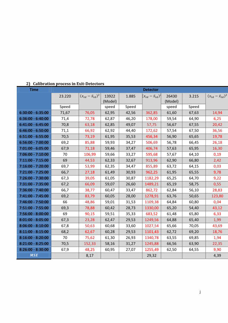
j

2) Calibration process in Exit-Detectors

Time Detector

23.220 13922 (Model)

1.885 26430 (Model)

3.215 26433 (Model)

Speed speed Speed speed Speed speed

6:30:00 - 6:35:00 71,67 76,05 62,95 42,56 362,85 61,60 67,63 14,94 63,76

6:36:00 - 6:40:00 71,4 72,78 62,87 46,20 178,00 59,54 64,90 6,25 62,40

6:41:00 - 6:45:00 70,8 63,18 62,85 49,07 57,75 56,67 67,55 20,42 63,03

6:46:00 - 6:50:00 71,1 66,92 62,92 44,40 172,62 57,54 67,50 36,56 61,45

6:51:00 - 6:55:00 70,5 73,19 61,95 35,53 456,34 56,90 65,65 19,78 61,20

6:56:00 - 7:00:00 69,2 85,88 59,93 34,27 506,69 56,78 66,45 26,18 61,33

7:01:00 - 6:05:00 67,9 71,18 59,46 37,47 406,74 57,63 65,95 16,30 61,91

7:06:00 - 7:10:00 70 106,99 59,66 33,27 595,68 57,67 64,10 0,19 63,67

7:11:00 - 7:15:00 69 44,53 62,33 32,67 913,96 62,90 66,80 2,42 65,25

7:16:00 - 7:20:00 69,7 53,99 62,35 34,47 855,89 63,72 64,15 0,03 63,97

7:21:00 - 7:25:00 66,7 27,18 61,49 30,93 962,25 61,95 65,55 9,78 62,42

7:26:00 - 7:30:00 67,3 39,05 61,05 30,87 1182,29 65,25 64,70 9,22 61,66

7:31:00 - 7:35:00 67,2 66,09 59,07 26,60 1489,21 65,19 58,75 0,55 59,49

7:36:00 - 7:40:00 66,7 38,77 60,47 33,47 862,72 62,84 56,10 28,83 61,47

7:41:00 - 7:45:00 69,2 83,79 60,05 28,00 1278,91 63,76 50,65 123,80 61,78

7:46:00 - 7:50:00 66 48,86 59,01 31,53 1109,38 64,84 60,80 0,04 60,99

7:51:00 - 7:55:00 69,3 78,88 60,42 28,73 1330,00 65,20 54,40 43,12 60,97

7:56:00 - 8:00:00 69 90,15 59,51 35,33 683,52 61,48 65,80 6,33 63,28

8:01:00 - 8:05:00 67,3 23,28 62,47 29,53 1249,56 64,88 65,40 1,99 63,99

8:06:00 - 8:10:00 67,8 50,63 60,68 33,60 1027,54 65,66 70,05 43,69 63,44

8:11:00 - 8:15:00 68,2 62,67 60,28 29,53 1101,43 62,72 69,20 18,76 64,87

8:16:00 - 8:20:00 70 75,62 61,30 26,93 1340,78 63,55 69,85 1,94 68,46

8:21:00 - 8:25:00 70,5 152,33 58,16 31,27 1245,88 66,56 63,90 22,35 68,63

8:26:00 - 8:30:00 67,9 48,25 60,95 27,07 1255,49 62,50 64,55 9,90 67,70

8,17 29,32 4,39

k

3) Comparison of Model Output and observation Speed in all detectors

50

52

54

56

58

60

62

64

66

68

70

0 5 10 15 20 25

Spe

ed

(km

/h)

Time series (5 minutes)

detector 23,205 (enctrance)

Observation

Model

l

10

20

30

40

50

60

70

80

0 5 10 15 20 25

Spe

ed

(km

/h)

Time series (5 minutes)

detector 1,845 (entrance

Observation

Model

0

10

20

30

40

50

60

70

80

0 5 10 15 20 25

Spe

ed

(km

/h)

Time series (5 minutes)

detector 3,270 (entrance)

Observation

Model

m

50

55

60

65

70

75

0 5 10 15 20 25

Spe

ed

(km

/h)

Time series (5 minutes)

detector 23,220 (exit)

Observation

Model

n

20

25

30

35

40

45

50

55

60

65

70

0 5 10 15 20 25

Spe

ed

(km

/h)

Time series (5 minutes)

detector 1,885 (exit)

Observation

Model

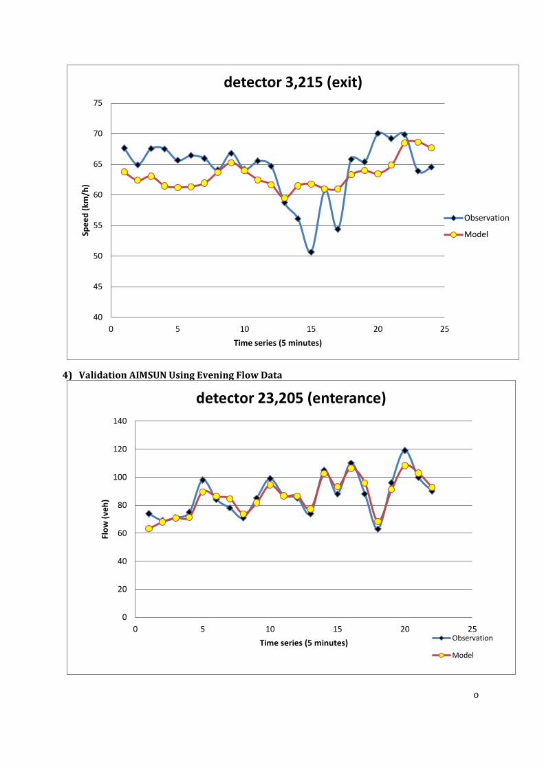
o

4) Validation AIMSUN Using Evening Flow Data

40

45

50

55

60

65

70

75

0 5 10 15 20 25

Spe

ed

(km

/h)

Time series (5 minutes)

detector 3,215 (exit)

Observation

Model

0

20

40

60

80

100

120

140

0 5 10 15 20 25

Flo

w (

veh

)

Time series (5 minutes)

detector 23,205 (enterance)

Observation

Model

p

220

240

260

280

300

320

340

0 5 10 15 20 25

Flo

w (

Ve

h)

Time series (5 minutes)

detector 1,845 (enterance)

Observation

Model

q

200

220

240

260

280

300

320

0 5 10 15 20 25

Flo

w (

Ve

h)

Time series (5 minutes)

detector 3,270 (enterance)

Observation Model

50

60

70

80

90

100

110

120

0 5 10 15 20 25

Flo

w (

Ve

h)

Time series (5 minutes)

detector 23,220 (exit)

Observation

Model

r

190

210

230

250

270

290

310

330

350

0 5 10 15 20 25

Flo

w (

Ve

h)

Time series (5 minutes)

detector 1,885 (exit)

Observation

Model

240

260

280

300

320

340

360

0 5 10 15 20 25

Flo

w (

Ve

h)

Time series (5 minutes)

detector 3,215 (exit)

Observation Model

s

C. SUMO CALIBRATION

1) Detector 1,845 No 1,845 observed 1,845 model (x1- x1')^2 (x2- x2')^2 (x3- x3')^2

x1 x2 x3 x1' x2' x3'

1 17,12 16,21 17,52 21,34259 19,02778 20,41667 17,8302882 7,939871605 8,390677778

2 17,36 16,48 17,9 21,77778 18,88889 20,61111 19,51676049 5,802745679 7,350123457

3 17,27 16,36 17,86 21,83333 18,33333 19,77778 20,82401111 3,894044444 3,677871605

4 14,71 15,32 17,73 21,27778 19,11111 20,94444 43,13570494 14,37252346 10,33265309

5 13,77 15,53 17,06 21,55556 19 20,72222 60,61487531 12,0409 13,4118716

6 14,17 15,82 17,74 21,61111 18,44444 20,22222 55,37013457 6,887708642 6,16142716

7 17,2 16,63 17,86 20,44444 18,05556 20,11111 10,52641975 2,032208642 5,067501235

8 17,34 16,66 17,87 21 18,94444 20,16667 13,3956 5,21868642 5,274677778

9 17,37 16,63 17,85 20,77778 18,27778 20,5 11,61294938 2,715171605 7,0225

10 17,35 16,63 17,83 21,22222 18,22222 19,44444 14,99410494 2,535171605 2,606430864

11 17,26 16,71 17,75 20,55556 18 20,11111 10,86068642 1,6641 5,574845679

12 17,37 16,56 17,85 20,05556 17,5 18,94444 7,212208642 0,8836 1,197808642

13 17,06 16,59 17,86 20,5 17,77778 19,61111 11,8336 1,410816049 3,066390123

14 14,95 16,25 17,76 20,72222 18,27778 20,27778 33,31854938 4,111882716 6,339204938

15 12,78 14,41 17,65 20,66667 18,38889 19,83333 62,19951111 15,83155679 4,766944444

16 13,57 14,37 17,68 19,77778 17,61111 19,05556 38,53650494 10,50480123 1,892153086

17 13,34 15,11 17,85 21 18,5 20,22222 58,6756 11,4921 5,627438272

18 13,78 15,93 17,89 20,38889 18,33333 19,72222 43,67741235 5,776011111 3,357038272

19 13,96 15,89 17,91 21,16667 18,88889 19,88889 51,93604444 8,993334568 3,916001235

20 13,36 14,69 17,6 12,05556 12,38889 17,55556 1,701575309 5,295112346 0,001975309

21 13,96 16,26 17,48 2,166667 2,722222 12,27778 139,0827111 183,2714272 27,06311605

22 13,79 16,21 17,45 2,277778 2,277778 12,44444 132,5312605 194,106816 25,05558642

23 12,53 13,78 17,39 2,277778 2,555556 10,44444 105,1080605 125,9881531 48,24074198

24 13,23 15,81 17,47 1,888889 2,222222 11,55556 128,6208012 184,6277049 34,98065309

Σ3 1093,115375 817,3964481 240,3756321

√Σ/n 6,74881278 5,835939114 3,164751386

t

2) Detector 23,205

No 23,205 observed 23,205 model (x1- x1')^2 (x2- x2')^2

x1 x2 x1' x2'

1 16,84 17,3 18,93519 18,47222 4,38980096 1,374104938

2 16,88 17,32 17,5 18,27778 0,3844 0,917338272

3 16,86 17,3 17,61111 18 0,564167901 0,49

4 16,91 17,32 16,61111 17,27778 0,089334568 0,001782716

5 16,97 17,3 17,33333 18,38889 0,132011111 1,185679012

6 17,02 17,25 17,83333 17,33333 0,661511111 0,006944444

7 16,84 17,33 17,27778 17,38889 0,191649383 0,003467901

8 16,93 17,29 17,16667 16,38889 0,056011111 0,812001235

9 16,91 17,36 16,66667 17,61111 0,059211111 0,06305679

10 16,93 17,28 16,66667 17,05556 0,069344444 0,050375309

11 16,82 17,3 16,16667 16,94444 0,426844444 0,126419753

12 16,9 17,3 16,27778 17,27778 0,387160494 0,000493827

13 16,96 17,29 17,27778 18,44444 0,100982716 1,332741975

14 16,87 17,31 17,05556 16,83333 0,034430864 0,227211111

15 16,94 17,37 17,16667 17,77778 0,051377778 0,166282716

16 16,9 17,27 16,88889 17,16667 0,000123457 0,010677778

17 16,85 17,35 16,72222 17,66667 0,01632716 0,100277778

18 16,83 17,32 16,44444 17,22222 0,148653086 0,009560494

19 16,94 17,32 17,05556 16,44444 0,013353086 0,766597531

20 16,98 17,27 16,94444 17,33333 0,001264198 0,004011111

21 16,91 17,31 16,55556 17,61111 0,125630864 0,090667901

22 16,97 17,3 17,5 17,77778 0,2809 0,228271605

23 16,94 17,3 17,38889 17,55556 0,201501235 0,065308642

24 16,95 17,35 17,44444 17,77778 0,244475309 0,182993827

Σ2 8,630466392 8,216266667

√Σ/n 0,599668881 0,58510208

u

3) Detector 3,270 No 3,270 observed 3,270 model (x1-

x1')^2 (x2-

x2')^2 (x3-

x3')^2 (x4-

x4')^2 x1 x2 x3 x4 x1' x2' x3' x4'

1 - - 18,39 15,28 - - 14,99 16,84 - - 11,55 2,44

2 - - 17,94 12,22 - - 14,85 16,88 - - 9,58 21,69

3 17,22 3,89 15,78 19,72 14,97 15,05 14,93 16,86 5,07 124,57 0,72 8,19

4 5,56 6,39 13,61 27,50 15,01 14,99 14,95 16,91 89,39 73,98 1,79 112,15

5 4,72 3,24 15,28 40,00 15,03 14,90 14,96 16,97 106,25 135,94 0,10 530,38

6 - 4,17 14,22 41,67 - 14,93 14,96 17,02 - 115,85 0,54 607,46

7 - 4,03 14,28 35,00 - 15,06 14,94 16,84 - 121,71 0,44 329,79

8 2,78 2,31 13,89 33,89 15,03 15,01 15,04 16,93 150,12 161,17 1,33 287,60

9 2,22 2,57 11,39 33,89 14,81 14,97 15,02 16,91 158,45 153,77 13,18 288,28

10 2,78 2,56 11,06 31,39 15,02 14,99 14,96 16,93 149,87 154,62 15,24 209,06

11 3,54 2,44 12,11 26,39 15,00 14,90 15,00 16,82 131,29 155,14 8,35 91,56

12 2,87 2,33 12,00 35,28 14,96 14,95 14,96 16,90 146,16 159,18 8,76 337,74

13 2,56 2,85 12,44 36,67 14,99 14,85 15,03 16,96 154,62 144,07 6,69 388,35

14 3,00 2,50 13,39 37,22 14,96 15,00 14,93 16,87 143,04 156,25 2,38 414,21

15 2,06 2,29 10,89 30,28 14,91 14,94 14,97 16,94 165,24 159,98 16,66 177,90

16 2,22 2,17 12,11 30,28 15,09 14,94 14,98 16,90 165,58 163,16 8,23 178,96

17 2,64 2,78 11,06 37,78 14,89 14,92 14,92 16,85 150,09 147,43 14,93 437,97

18 2,43 2,29 10,17 26,39 14,92 15,08 14,98 16,83 155,99 163,54 23,17 91,37

19 2,61 1,94 12,67 24,44 14,90 14,94 15,05 16,94 151,02 168,88 5,68 56,32

20 2,41 2,31 9,78 30,28 15,09 15,06 14,97 16,98 160,85 162,44 26,96 176,83

21 2,36 2,85 12,67 32,50 14,95 14,94 14,92 16,91 158,48 146,24 5,08 243,05

22 2,22 1,39 9,33 22,22 14,93 14,89 14,98 16,97 161,49 182,28 31,88 27,59

23 2,41 3,06 12,11 29,44 14,89 14,93 15,02 16,94 155,82 141,00 8,46 156,36

24 2,78 2,22 11,72 33,33 14,95 15,02 14,97 16,95 148,16 163,78 10,55 268,41

Σ1 2.806,96 3.254,98 232,24 5.443,68

√Σ/n 10,81 11,65 3,11 15,06