comparison of the modified biot-gassmann theory and … of the modified biot-gassmann theory and the...

Comparison of the Modified Biot-Gassmann Theory and the Kuster-Toksöz Theory in Predicting Elastic Velocities of Sediments

Scientific Investigations Report 2008–5196

U.S. Department of the InteriorU.S. Geological Survey

V kp = + 4 3/

EI

kma

ma

ma

2 63

44 34

=−

+

()(

)T F

Fiijj = 3

1

2


By Myung W. Lee

Scientific Investigations Report 2008–5196

U.S. Department of the InteriorU.S. Geological Survey

U.S. Department of the InteriorDIRK KEMPTHORNE, Secretary

U.S. Geological SurveyMark D. Myers, Director

U.S. Geological Survey, Reston, Virginia: 2008

For product and ordering information: World Wide Web: http://www.usgs.gov/pubprod Telephone: 1-888-ASK-USGS

For more information on the USGS—the Federal source for science about the Earth, its natural and living resources, natural hazards, and the environment: World Wide Web: http://www.usgs.gov Telephone: 1-888-ASK-USGS

Any use of trade, product, or firm names is for descriptive purposes only and does not imply endorsement by the U.S. Government.

Although this report is in the public domain, permission must be secured from the individual copyright owners to reproduce any copyrighted materials contained within this report.

Suggested citation:Lee, M.W., 2008, Comparison of the modified Biot-Gassmann theory and the Kuster-Toksöz theory in predicting elastic velocities of sediments: U.S. Geological Survey Scientific Investigations Report 2008–5196, 14 p.

iii

ContentsAbstract ...........................................................................................................................................................1Introduction.....................................................................................................................................................1Theory ............................................................................................................................................................................. 2

Modified Biot-Gassmann Theory ......................................................................................................2Kuster-Toksöz Theory ...........................................................................................................................2Moduli of Dry Frame .............................................................................................................................3

Modeling..........................................................................................................................................................4Modified Biot-Gassmann Theory ............................................................................................................4Kuster and Toksöz Theory .........................................................................................................................4

Discussion .......................................................................................................................................................4Kuster and Toksöz Theory With and Without Gassmann Theory .................................................4Comparison of Kuster and Toksöz-Gassmann Theories and Modified

Biot-Gassmann Theory of Lee ...............................................................................................6Predicting S-Wave Velocity ................................................................................................................8Pore Aspect Ratios ...............................................................................................................................9Parameters of Modified Biot-Gassmann Theory and Pore Aspect Ratio

of Kuster-Toksöz Theory .......................................................................................................11Conclusions...................................................................................................................................................13References Cited..........................................................................................................................................13

Figures 1. P-wave velocities predicted by modified Biot-Gassmann theory

and by Kuster-Toksöz theory .......................................................................................................5 2. Modeled P- and S-wave velocities with respect to pore aspect ratio ................................6 3. Modeled velocities using Kuster-Toksöz theory and Kuster-Toksöz

theory–Gassmann theory ............................................................................................................7 4. Measured P- and S-wave velocities compared with predicted velocities

for semiconsolidated sediments using modified Biot-Gassmann theory and Kuster-Toksöz theory–Gassmann theory ..........................................................................8

5. Measured P- and S-wave velocities compared with predicted velocities for consolidated sandstones using Kuster-Toksöz theory–Gassmann theory ..............................................................................................................................................9

6. Measured P- and S-wave velocities compared with predicted velocities for consolidated sandstones using modified Biot-Gassmann theory ................................10

7. Well log P- and S-wave velocities compared with predicted velocities using modified Biot-Gassmann theory and Kuster-Toksöz theory–Gassmann theory ..........................................................................................................11

8. Measured and predicted S-wave velocities at Alpine–1 well, North Slope of Alaska ...........................................................................................................................12

9. Measured and predicted porosity reduction with respect to effective pressure .......................................................................................................................................12

Table 1. Elastic constants used in velocity models ................................................................................5

iv

Abbreviations Used in This ReportBGT Biot-Gassmann theoryBGTL modified Biot-Gassmann theory of LeeKTT Kuster-Toksöz theoryKTT–GM Kuster-Toksöz theory–Gassmann theoryGPa gigapascal (109 pascal)km/s kilometer per secondMPa megapascal

Conversion Factors

Multiply By To obtainGPa 9,869 atmospherekm/s 0.621 mile per secondMPa 9.869 atmosphere

AbstractElastic velocities of water-saturated sandstones depend

primarily on porosity, effective pressure, and the degree of consolidation. If the dry-frame moduli are known, from either measurements or theoretical calculations, the effect of pore water on velocities can be modeled using the Gassmann theory. Kuster and Toksöz (1974, Geophysics, v. 39, p. 587–606) developed a theory based on wave-scattering theory for a variety of inclusion shapes, which provides a means for calculating dry- or wet-frame moduli. In the Kuster-Toksöz theory, elastic wave velocities through different sediments can be predicted by using different aspect ratios of the sediment’s pore space. Elastic velocities increase as the pore aspect ratio increases (larger pore aspect ratio describes a more spherical pore). On the basis of the velocity ratio, which is assumed to be a function of (1–)n, and the Biot-Gassmann theory, Lee (2002, Geophysics, v. 67, p. 1711–1719) developed a semi-empirical equation for predicting elastic velocities, which is referred to as the modified Biot-Gassmann theory of Lee. In this formulation, the exponent n, which depends on the effective pressure and the degree of consol-idation, controls elastic velocities; as n increases, elastic velocities decrease. Computationally, the role of exponent n in the modified Biot-Gassmann theory by Lee is similar to the role of pore aspect ratios in the Kuster-Toksöz theory. For consolidated sediments, either theory predicts accurate velocities. However, for uncon-solidated sediments, the modified Biot-Gassmann theory by Lee performs better than the Kuster-Toksöz theory, particularly in predicting S-wave velocities.

IntroductionNumerous studies relate physical properties of rock to

geophysical observations. A brief review is provided here, and a more comprehensive discussion is given by Mavko and others (1998), who brought together much of the theory and the data forming the foundation of rock physics.

Biot (1956) developed theoretical formulas for predicting the frequency-dependent elastic velocities of water-saturated rocks in all frequency ranges, and Geertsma and Smit (1961) analyzed the Biot equation for dilatational waves in the low-frequency range.

Gassmann (1951) derived equations for elastic velocities of the fluid-saturated porous media at zero frequency. The Gassmann (1951) theory predicts the bulk modulus of the fluid-saturated porous medium from the known bulk moduli of the frame and the pore fluid, and it assumes that the sediment shear modulus is not affected by fluid saturation. The essential input for the application of the Gassmann equation is the bulk modulus of the dry frame, which is generally measured in the laboratory. These theories are generally applied to consolidated sediments at high effective pressure, and some empirical formulas also have been developed (for example, Wyllie and others, 1956; Raymer and others, 1980; Castagna and others, 1985; Han and others, 1986).

Moduli of dry sediments or water-saturated sediments can be calculated from the Kuster and Toksöz (1974) theory (KTT), which is based on wave scattering theory. On the basis of KTT and differential effective medium theory, Xu and White (1996) proposed a method of calculating elastic velocities using pore aspect ratios to characterize the compli-ance of sand and clay components. In KTT, as the pore aspect ratio increases, elastic velocities increase, so that the effect on velocities of effective pressure and the degree of con-solidation can be modeled using various pore aspect ratios. Because elastic velocities depend on pore aspect ratios, KTT can be used for both consolidated and unconsolidated sedi-ments. Also, KTT predicts that shear modulus varies with fluid saturation, which differs from the prediction of the Biot-Gassmann theory (BGT) (Thomsen, 1985).

Theories for velocities of unconsolidated sediments have been introduced: for example, the effective medium theory by Helgerud and others (1999) and Jakobsen and others (2000), and the modified Biot-Gassmann theory of Lee (herein referred to as BGTL) by Lee (2002, 2003). In BGTL, the shear modulus of water-saturated sediments is derived under the assumption that S-wave velocity (V

s ) is related to the P-wave velocity (V

p )

by G(1 – ) n, where G is a scalar and is porosity. Parameter n is introduced to incorporate the effect of effective pressure and the degree of consolidation on elastic velocities, and parameter G is introduced to compensate for the discrepancy between the observed V

p /V

s ratio of sediment and V

p /V

s ratio of the grains.

In BGTL, as n increases, elastic velocities decrease; the effect on velocities of effective pressure and degree of consolidation is modeled using various values of n.


By Myung W. Lee

2 Comparison of Modified Biot-Gassman Theory and Kuster-Toksöz Theory

Because the pore aspect ratios in KTT and the exponent n in BGTL have a similar effect on predicted velocity, the per-formance of KTT and BGTL is compared in this paper with a variety of measured velocities for consolidated sandstones and unconsolidated sands and with well log velocities at the Alpine–1 well, North Slope of Alaska.

Theory

Modified Biot-Gassmann Theory

Lee (2003) derived a sediment shear modulus based on the assumption that V

s=V

pG(1–)n, where is the V

s /V

p ratio

of the grain and is porosity. G and n are parameters depend-ing on effective pressure, consolidation, and clay content. The shear modulus is given by

=− − + −

+ − −ma ma

nma

n

ma ma

k G MGk G

( ) ( ) ( )[ ( )

1 1 14 1 1

2 2 2 2 2

2 2

nn ]/ 3

, (1)

where

1M k kma fl

=−

+( ) ,

and kma

, µma

, kfl, , and ß are the bulk and shear moduli of the

matrix, the bulk modulus of the fluid, porosity, and the Biot coefficient, respectively.

For the sediment bulk modulus, the Biot-Gassmann theory (BGT) gives

k k Mma= − +( )1 2 . (2)

Elastic velocities in water-saturated sediments can be com-puted from the elastic moduli by the following:

Vk

p =+ 4 3/ and Vs = , (3)

where is density of the formation given by = (1 – )ma

+ fl,

and ma

and fl are the matrix and pore fluid densities, respec-

tively. Lee (2002) referred to the use of equations 1 and 2 for the computation of elastic velocities as the modified Biot-Gassmann theory by Lee.

For modeling soft rocks or unconsolidated sediments, the following Biot coefficient is used (Lee, 2002):

=−

+++

183 051

0 994940 56468 0 10817

..( . ) / .e

. (4)

For modeling hard or consolidated formations, the equation by Raymer and others (1980) is used, as written in the following form by Krief and others (1990):

= 1 – (1 – )3.8. (5)

According to Lee (2003), the exponent n is given by

n = [10(0.426–0.235Log10 p)]/m (6a)

with

m = 1.0 + 4.95e5212/p (6b)

and G is given by

G = 0.9552 + 0.0448e–Cv /0.06714 (7)

where p is effective pressure in megapascals (MPa),

m is a constant related to the degree of consolidation,

and C

v is the clay volume in decimal units.

For a detailed discussion of parameters n and G, consult Lee (2003).

In order to accurately model the degree of consolidation in the framework of BGTL, the following geometric mean of Biot coefficient is used (Lee, 2005), which is appropriate for sediments between consolidated and unconsolidated—that is, those that are semiconsolidated or loosely consolidated as mentioned by Blangy and others (1993):

= 1

21– (8)

where 1 is the Biot coefficient for unconsolidated

sediments (equation 4),

2 is the Biot coefficient for consolidated sediments (equation 5),

and is a weight.

The mean Biot coefficient is just the Biot coefficient for uncon-solidated sediments when = 1, and is the Biot coefficient for consolidated sediments when = 0.

Kuster-Toksöz Theory

The Kuster-Toksöz theory (Kuster and Toksöz, 1974) is based on the long wavelength, first-order scattering phenom-ena of elastic waves in a two-phase medium. The medium is assumed to consist of matrix and inclusions. The effective elastic moduli of a two-phase medium that contains ellipsoidal inclusions can be written as follows:

k k k kkk

Td ma mad ma

ma mal iijj l

l s c

− = −++ =

∑13

3 43 4

( ) ( )*

,

(9)

and

d mad ma ma ma ma ma ma

ma ma ma

k kk

− =− + + +

+6 2 9 8

5 3 4( )( ) ( )

( )

*

l ijij liijj l

l s c

TT

( )( )

.,

−

=∑ 3 (10)

In equations 9 and 10, kd, k

ma, and k* are the bulk

moduli of the dry frame, the grain, and the pore inclusion material, respectively;

d,

ma, and * are the shear

moduli of the dry frame, the grain, and the pore inclusion material, respectively. Porosity () is assumed to consist of

Theory 3

stiff pores (s) with a pore aspect ratio

s in sandstone and

compliant or soft pores (c) with a pore aspect ratio

c in

shale. The pore aspect ratios cannot be measured directly and their estimation relies on the best fit to log or laboratory obser-vations (Xu and White, 1996). T

ijkl is a fourth-order tensor

that relates the uniform strain field to the strain field within an elastic inclusion.

The pore aspect ratio functions Tiijj

and Tijij

are expressed as follows:

TFFiijj =3 1

2

(11)

and

F TT

F FF F F F F F

F Fijijiijj≡ − = + +

+ −( )

( )

32 1

3 4

4 5 6 7 8 9

2 4

(12)

where

F A g Rg

1 132

32

52

43

= + + − + −

( ) ( )

F Ag R g

AA B R g

B R2 1 13

23 52

23 3 4

3 4= + ++

−+

+ − + −

+ −

+

( ) ( )

( ) (

( )

rr g( )− + 2 2

F A R g R3

2

21 21

1= + − ++

−

( )

( )( )

F A g R g4 1 3= + + − −[ ]( ) (13)

F A R g g B R5 4 3 3 4= + − −[ ] + −( / ) ( )

F A g R g B R6 1 1 1 3 4= + + − +[ ] + − −( ) ( )( )

F A g R g B R7 2 9 3 5 3 3 4= + + − +[ ] + −( ) ( )

F A R g R R B R8 1 2 1 2 5 3 2 1 3 4= − + − + −[ ] + − −( ) / ( ) / ( )( )

F A g R R B R9 1 3 4= − −[ ] + −( ) ( )

A Bkk

Rk

g

ma ma

ma

ma ma

= − = −

=+

=−

* * *

, , ,

(

113

33 4

13

2

2

− =−

− −

−21

12 3 21 2),

( )cos ( )/

.

KTT assumes that the pores are isolated and do not interact, which leads to the restriction that the pore concentra-tion is dilute (that is, /<<1). Differential effective medium theory (Cleary and others, 1980) is used to overcome this limitation by incrementally adding the pores in small steps in such a way that the noninteraction criterion is satisfied in each step (Mavko and others, 1998; Keys and Xu, 2002). Beginning with solid rock, KTT is used to compute the effective medium that results from adding a small set of pores to the matrix. The process is repeated, using the effective medium from the previ-ous calculation as the rock matrix for the next calculation until the total pore volume has been added to the rock.

For water-saturated sediments with ellipsoidal pore aspect ratios, KTT shown in equations 9 through 13 can be used in two ways: (1) to calculate the moduli of water-saturated sedi-ments by using the bulk modulus of water for k* in equation 13 (referred to as KTT in this paper), or (2) to calculate the moduli for dry rock with k* = 0 in equation 13 and to use Gassmann theory for water-saturated sediments (referred to as KTT–GM). Because the inclusions are isolated with respect to wave propagation, KTT simulates the behavior of very high frequency saturated rock appropriate to ultrasonic laboratory conditions (Mavko and others, 1998). At low frequencies, KTT–GM is preferred to KTT.

One particularly useful aspect of KTT is that it pre-dicts the S-wave velocity in sediments with differing fluid saturation, which is not consistent with the prediction of the BGT. Equations 10 and 12 indicate that the shear modulus of fluid-saturated sediments is calculated using the function F, which is related to the bulk modulus of the fluid through the constant B shown in equation 13.

Moduli of Dry Frame

In the framework of the BGT, the dry frame bulk modulus (k

d) is given by the following formula by substituting M = 0 in

equation 2:

kd = k

ma(1 – ). (14a)

In the framework of BGTL, the following shear modulus of dry frame (

d) can be derived from equation 1 with M = 0 and

n ≈ 0 under the assumption that the velocity ratio of a dry rock is almost constant irrespective of porosity (Pickett, 1963).

d

ma ma

ma ma

k Gk G

≈−

+ −( )( ) /1

4 1 3

2

2. (14b)

In the clay-free case in which G = 1, equation 14b is identical to the formula derived by Krief and others (1990), which means that the velocity ratio of a dry rock is identical to that of the matrix. It is noted that when G = 1, the ratio of k

d /

d depends

only on the sediment grains (that is, kma

/ ma

). However, when G 1.0, the ratio of k

d /

d also depends on G. It is noted that

even though bulk and shear moduli depend on the Biot coef-ficient and the Biot coefficient depends on porosity, the ratio of k

d /

d is independent of the Biot coefficient or porosity.


In KTT, the bulk and shear moduli of a dry frame with the aspect ratio of 1.0 are given by the following (Toksöz and others, 1976):

kkkd

KTT ma

ma ma

=−

+( )/( )

11 3 4

(15a)

dktt ma

ma ma ma mak k=

−+ + +

( )( ) /( )

11 6 2 9 8

(15b)

In KTT, kdKTT /

dKTT depends explicitly on porosity, which

means that the velocity ratio of dry rock is not a constant. The effect of effective pressure on the velocity ratio can be incor-porated implicitly through the pore aspect ratio.

Modeling

Modified Biot-Gassmann Theory

In the framework of BGTL, the magnitude of elastic velocities in water-saturated sediments depends primarily on the exponent n and the Biot coefficient. The exponent n depends on effective pressure and the rate of porosity reduc-tion with respect to effective pressure. The Biot coefficient depends on porosity, the degree of consolidation, and effective pressure. As shown in equation 8, the geometric average of the end member Biot coefficient can be used for semiconsolidated or loosely consolidated sediments as described by Blangy and others (1993).

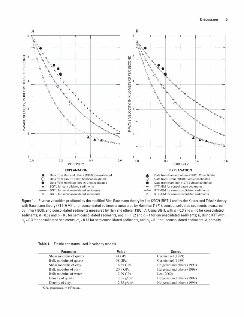
Figure 1A shows three velocity trends with respect to porosities for clean consolidated, unconsolidated, and semi-consolidated sediments. Relevant elastic constants used in all models are shown in table 1. P-wave velocities for the (1) consolidated sediment are derived from BGTL, with n = 0.3, C

v = 0.0, and = 0 (which uses the Biot coefficient

given in equation 5); (2) unconsolidated sediment are derived from BGTL, with n = 1.4, C

v = 0.0, and = 1 (which uses the

Biot coefficient given in equation 4); and (3) semiconsolidated sediment are derived from BGTL, with n = 0.52, C

v = 0.0,

and = 0.5. The three data sets can be readily compared in figure 1A.

For a given Biot coefficient, BGTL contains two adjust-able parameters (n and G). As shown in figure 1A, different Biot coefficients and n are used to model velocities of three sets of sediments having differing degrees of consolidation; the velocity decreases as n increases. Equation 6 indicates that n depends on effective pressure and a constant m, which is related to the porosity change with respect to effective pressure (Lee, 2003). However, in practice the porosity change with respect to effective pressure is rarely known. Therefore, the exponent n or parameter m can be treated as a free parameter to fit the measured velocities in BGTL.

The porosity ranges shown in figure 1A should be inter-preted carefully, because for porosities less than the critical porosity, the mineral grains are load bearing; for porosities greater than the critical porosity, the grains are in suspension (Nur and others, 1998). Therefore, porosities of consolidated or semiconsolidated sediments cannot be greater than the criti-cal porosity, which is about 40 percent.

Kuster and Toksöz Theory

In KTT, the pore aspect ratio controls the velocity. For a given porosity, the velocity increases as the aspect ratio increases. Velocities modeled using KTT–GM are shown in figure 1B. For these plots, velocities are calculated for con-solidated sediments with

s = 0.3, those for semiconsolidated

sediments with s = 0.18, and those for unconsolidated

sediments with s = 0.1. The clay content, C

v, is assumed

to be zero in all cases, and if shaly sandstones are used for the modeling, the pore aspect ratio related to clay should be included.

As in figure 1A, three measured data sets are shown in figure 1B along with the calculated velocities. The predicted velocities closely follow the measured velocities. However, even though the predicted velocities obtained from KTT–GM and BGTL agree well with measured velocities, the predicted velocities from BGTL differ slightly from those predicted by KTT–GM when they are extrapolated to other porosi-ties. For example, for consolidated sediments, BGTL with n = 0.3 predicts V

p = 3.5 km/s at = 0.3, whereas KTT–GM

predicts Vp = 3.8 km/s. As mentioned previously, compari-

sons between BGTL and KTT–GM for consolidated and semiconsolidated sediments are valid for porosities less than about 40 percent.

Discussion

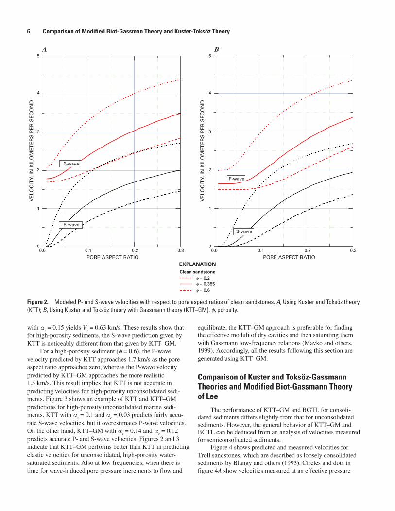
Kuster and Toksöz Theory With and Without Gassmann Theory

For a given porosity, velocities are calculated with respect to the pore aspect ratio. It is shown that for a given porosity and pore aspect ratio, velocities predicted by KTT are higher than those predicted by KTT–GM (fig. 2). Model results indicate that for consolidated sediments, both KTT and KTT–GM can be used to accurately predict P-wave velocities. For example, KTT with

s = 0.2 predicts a P-wave velocity of

4 kilometers per second (km/s) for a sediment with = 0.2, as does KTT–GM if

s = 0.22. Similar results are obtained

for S-wave velocities. For an unconsolidated sediment with = 0.6, KTT with

s = 0.05 predicts V

p = 1.76 km/s, as does

KTT–GM with s = 0.15. However, for S-wave velocities,

KTT with s = 0.05 yields V

s = 0.24 km/s, whereas KTT–GM

Discussion 5

EXPLANATIONData from Han and others (1986): ConsolidatedData from Timur (1968): SemiconsolidatedData from Hamilton (1971): UnconsolidatedBGTL for consolidated sedimentsBGTL for semiconsolidated sedimentsBGTL for semiconsolidated sediments

EXPLANATIONData from Han and others (1986): ConsolidatedData from Timur (1968): SemiconsolidatedData from Hamilton (1971): UnconsolidatedKTT–GM for consolidated sedimentsKTT–GM for semiconsolidated sedimentsKTT–GM for semiconsolidated sediments

P-W

AV

E V

ELO

CIT

Y, IN

KIL

OM

ET

ER

S P

ER

SE

CO

ND

P-W

AV

E V

ELO

CIT

Y, IN

KIL

OM

ET

ER

S P

ER

SE

CO

ND

POROSITY POROSITY

A B6

5

4

3

2

1

6

5

4

3

2

10.0 0.2 0.4 0.6 0.0 0.2 0.4 0.6

Figure 1. P-wave velocities predicted by the modified Biot-Gassmann theory by Lee (2002) (BGTL) and by the Kuster and Toksöz theory with Gassmann theory (KTT–GM) for unconsolidated sediments measured by Hamilton (1971), semiconsolidated sediments measured by Timur (1968), and consolidated sediments measured by Han and others (1986). A, Using BGTL with n = 0.3 and = 0 for consolidated sediments, n = 0.52 and = 0.5 for semiconsolidated sediments, and n = 1.02 and = 1 for unconsolidated sediments; B, Using KTT with s = 0.3 for consolidated sediments, s = 0.18 for semiconsolidated sediments, and s = 0.1 for unconsolidated sediments. , porosity.

Table 1. Elastic constants used in velocity models.

Parameter Value SourceShear modulus of quartz 44 GPa1 Carmichael (1989)Bulk modulus of quartz 38 GPa Carmichael (1989)Shear modulus of clay 6.85 GPa Helgerud and others (1999)Bulk modulus of clay 20.9 GPa Helgerud and others (1999)Bulk modulus of water 2.29 GPa Lee (2002)Density of quartz 2.65 g/cm3 Helgerud and others (1999)Density of clay 2.58 g/cm3 Helgerud and others (1999)

1GPa, gigapascal, = 109 pascal


with s = 0.15 yields V

s = 0.63 km/s. These results show that

for high-porosity sediments, the S-wave prediction given by KTT is noticeably different from that given by KTT–GM.

For a high-porosity sediment ( = 0.6), the P-wave velocity predicted by KTT approaches 1.7 km/s as the pore aspect ratio approaches zero, whereas the P-wave velocity predicted by KTT–GM approaches the more realistic 1.5 km/s. This result implies that KTT is not accurate in predicting velocities for high-porosity unconsolidated sedi-ments. Figure 3 shows an example of KTT and KTT–GM predictions for high-porosity unconsolidated marine sedi-ments. KTT with

s = 0.1 and

c = 0.03 predicts fairly accu-

rate S-wave velocities, but it overestimates P-wave velocities. On the other hand, KTT–GM with

s = 0.14 and

c = 0.12

predicts accurate P- and S-wave velocities. Figures 2 and 3 indicate that KTT–GM performs better than KTT in predicting elastic velocities for unconsolidated, high-porosity water-saturated sediments. Also at low frequencies, when there is time for wave-induced pore pressure increments to flow and

equilibrate, the KTT–GM approach is preferable for finding the effective moduli of dry cavities and then saturating them with Gassmann low-frequency relations (Mavko and others, 1999). Accordingly, all the results following this section are generated using KTT–GM.

Comparison of Kuster and Toksöz-Gassmann Theories and Modified Biot-Gassmann Theory of Lee

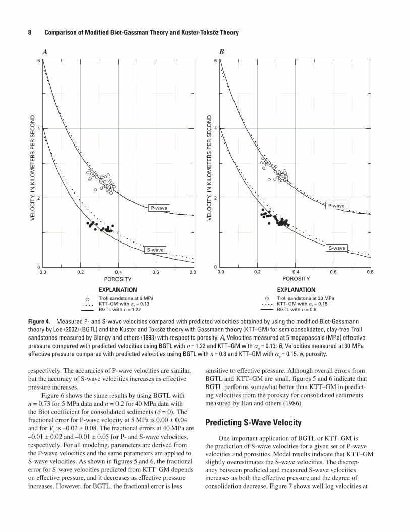
The performance of KTT–GM and BGTL for consoli-dated sediments differs slightly from that for unconsolidated sediments. However, the general behavior of KTT–GM and BGTL can be deduced from an analysis of velocities measured for semiconsolidated sediments.

Figure 4 shows predicted and measured velocities for Troll sandstones, which are described as loosely consolidated sediments by Blangy and others (1993). Circles and dots in figure 4A show velocities measured at an effective pressure

EXPLANATION

= 0.2 = 0.385 = 0.6

Clean sandstone

P-wave

S-wave

P-wave

S-wave

5

4

3

2

1

0

5

4

3

2

1

00.0 0.2 0.30.1 0.0 0.2 0.30.1

VE

LOC

ITY,

IN K

ILO

ME

TE

RS

PE

R S

EC

ON

D

VE

LOC

ITY,

IN K

ILO

ME

TE

RS

PE

R S

EC

ON

D

PORE ASPECT RATIO PORE ASPECT RATIO

A B

Figure 2. Modeled P- and S-wave velocities with respect to pore aspect ratios of clean sandstones. A, Using Kuster and Toksöz theory (KTT); B, Using Kuster and Toksöz theory with Gassmann theory (KTT–GM). , porosity.

Discussion 7

of 5 MPa; solid lines are predicted velocities using BGTL with n = 1.22, = 0.5, and C

v = 0.0; and dotted lines are pre-

dicted velocities using KTT–GM with s = 0.13 and C

v = 0.0.

Predicted P-wave velocities from BGTL and KTT–GM agree well with the measured V

p. However, KTT–GM

overestimates Vs, whereas V

s from BGTL agrees well with

the measured Vs. Figure 4B shows measured and predicted

velocities of Troll sandstones at the effective pressure of 30 MPa—solid lines are predicted velocities using BGTL with n = 0.8, = 0.5, and C

v = 0.0; and dotted lines are

predicted velocities using KTT–GM with s = 0.15 and

Cv = 0.0. The same conclusions can be drawn from model

results regarding measured and predicted velocities at both effective pressures.

Because velocities depend on effective pressure, the parameter n in BGTL changes from n = 1.22 at 5 MPa to n = 0.8 at 30 MPa, whereas the parameter

s in KTT–GM

changes from s = 0.13 at 5 MPa to

s = 0.15 at 30 MPa.

Figure 4 also indicates that the predicted Vs from KTT–GM

is generally greater than the measured Vs, but the difference

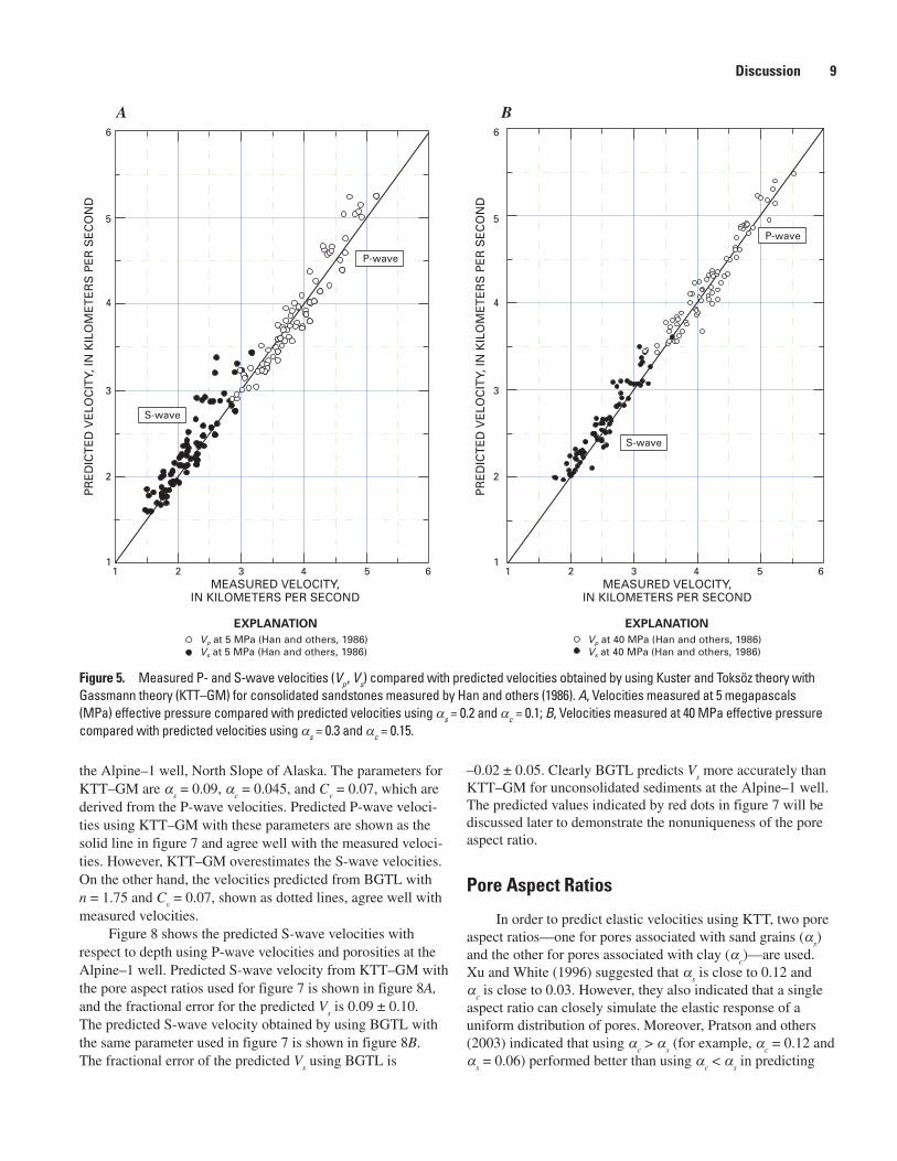
decreases as effective pressure increases.Figures 5 and 6 show velocities of consolidated

sediments measured by Han and others (1986). Figure 5 is a plot of velocities predicted from porosity and clay volume content by using KTT–GM. For data at 5 MPa (fig. 5A), the values of

s = 0.2 and

c = 0.1 are

used. Fractional errors for the predicted Vp are 0.00 ± 0.04

and 0.07 ± 0.08 for Vs, indicating that KTT–GM predicts

P-wave velocities more accurately than S-wave velocities. However, the inaccuracy in the S-wave velocity results from adjusting the pore aspect ratios to fit the P-wave velocities. For 40 MPa data (fig. 5B),

s = 0.3 and

c = 0.15 are used

for KTT–GM. The fractional errors are 0.01 ± 0.04 and 0.04 ± 0.05 for the predicted P-wave and S-wave velocities,

Vp from Hamilton (1971)Vs from Hamilton (1971)KTTBGTL

Vp from Hamilton (1971)Vs from Hamilton (1971)KTT–GMBGTL

POROSITY POROSITY

VE

LOC

ITY,

IN K

ILO

ME

TE

RS

PE

R S

EC

ON

D

VE

LOC

ITY,

IN K

ILO

ME

TE

RS

PE

R S

EC

ON

D

3

2

1

0

3

2

1

00.0 0.2 0.60.4 0.8 1.0 0.0 0.2 0.60.4 0.8 1.0

A B

P-wave

S-wave

P-wave

S-wave

EXPLANATION EXPLANATION

Figure 3. Modeled velocities obtained by using Kuster and Toksöz theory (KTT) and Kuster and Toksöz theory with Gassmann theory (KTT–GM), both compared with modified Biot-Gassmann theory by Lee (BGTL) with n = 0.8 and Cv = 0.3 with respect to porosity for unconsolidated sediment measured by Hamilton (1971). P-wave velocities (Vp) are measured velocities, but S-wave velocities (Vs) are computed velocities. A, Using KTT with s = 0.1, c = 0.03, and Cv = 0.3; B, Using KTT–GM with s = 0.14, c = 0.12, and Cv = 0.3. , porosity.


respectively. The accuracies of P-wave velocities are similar, but the accuracy of S-wave velocities increases as effective pressure increases.

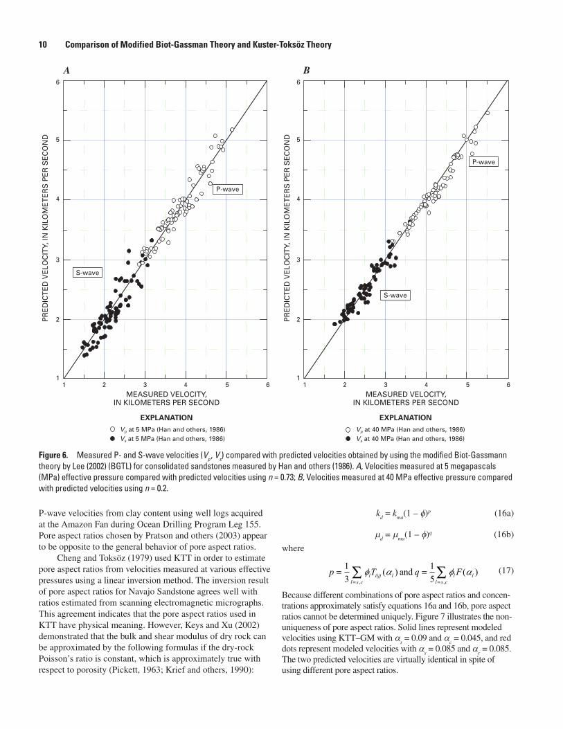
Figure 6 shows the same results by using BGTL with n = 0.73 for 5 MPa data and n = 0.2 for 40 MPa data with the Biot coefficient for consolidated sediments ( = 0). The fractional error for P-wave velocity at 5 MPa is 0.00 ± 0.04 and for V

s is –0.02 ± 0.08. The fractional errors at 40 MPa are

–0.01 ± 0.02 and –0.01 ± 0.05 for P- and S-wave velocities, respectively. For all modeling, parameters are derived from the P-wave velocities and the same parameters are applied to S-wave velocities. As shown in figures 5 and 6, the fractional error for S-wave velocities predicted from KTT–GM depends on effective pressure, and it decreases as effective pressure increases. However, for BGTL, the fractional error is less

sensitive to effective pressure. Although overall errors from BGTL and KTT–GM are small, figures 5 and 6 indicate that BGTL performs somewhat better than KTT–GM in predict-ing velocities from the porosity for consolidated sediments measured by Han and others (1986).

Predicting S-Wave Velocity

One important application of BGTL or KTT–GM is the prediction of S-wave velocities for a given set of P-wave velocities and porosities. Model results indicate that KTT–GM slightly overestimates the S-wave velocities. The discrep-ancy between predicted and measured S-wave velocities increases as both the effective pressure and the degree of consolidation decrease. Figure 7 shows well log velocities at

Figure 4. Measured P- and S-wave velocities compared with predicted velocities obtained by using the modified Biot-Gassmann theory by Lee (2002) (BGTL) and the Kuster and Toksöz theory with Gassmann theory (KTT–GM) for semiconsolidated, clay-free Troll sandstones measured by Blangy and others (1993) with respect to porosity. A, Velocities measured at 5 megapascals (MPa) effective pressure compared with predicted velocities using BGTL with n = 1.22 and KTT–GM with s = 0.13; B, Velocities measured at 30 MPa effective pressure compared with predicted velocities using BGTL with n = 0.8 and KTT–GM with s = 0.15. , porosity.

EXPLANATIONTroll sandstone at 5 MPaKTT–GM with s = 0.13BGTL with n = 1.22

EXPLANATIONTroll sandstone at 30 MPaKTT–GM with s = 0.15BGTL with n = 0.8

POROSITYPOROSITY

VE

LOC

ITY,

IN K

ILO

ME

TE

RS

PE

R S

EC

ON

D

VE

LOC

ITY,

IN K

ILO

ME

TE

RS

PE

R S

EC

ON

D

0.0 0.00.2 0.4 0.6 0.8

6

4

2

00.2 0.4 0.6 0.8

6

4

2

0

P-wave

S-wave

P-wave

S-wave

A B

Discussion 9

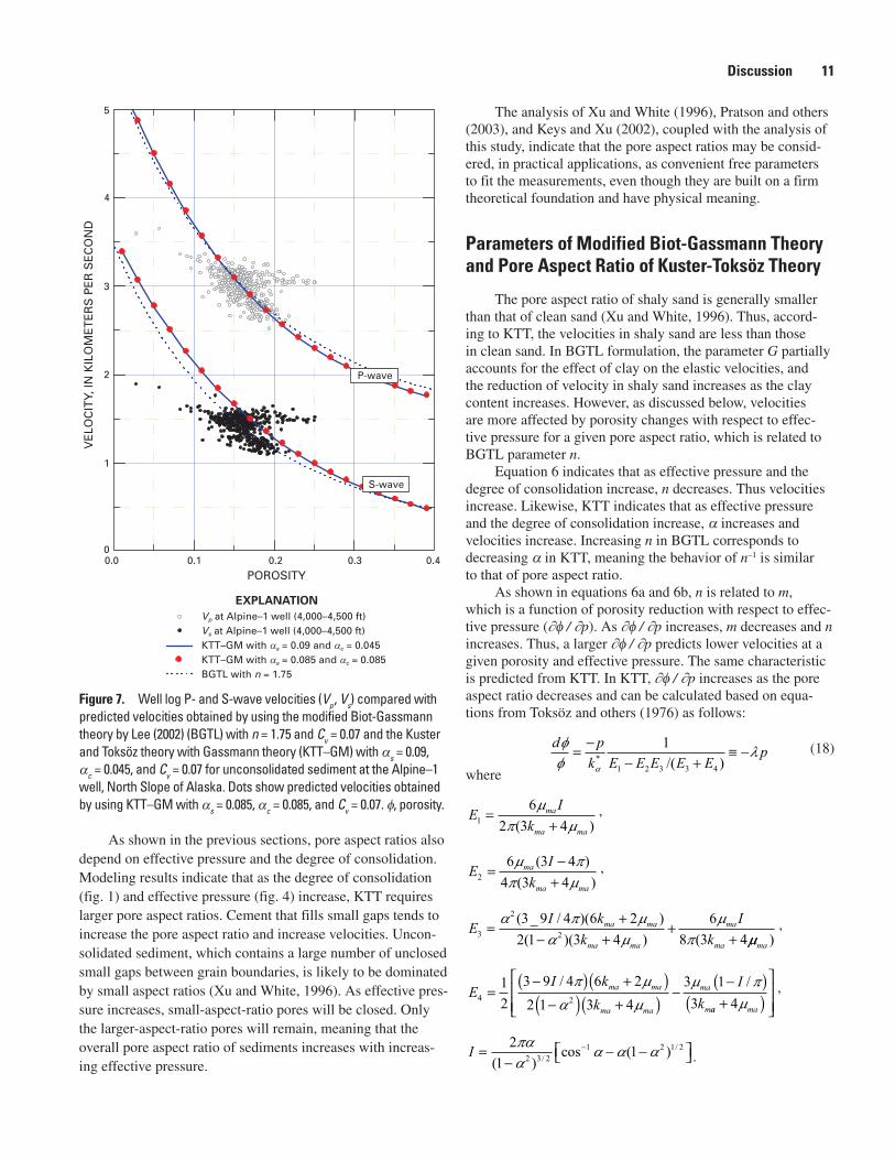
the Alpine–1 well, North Slope of Alaska. The parameters for KTT–GM are

s = 0.09,

c = 0.045, and C

v = 0.07, which are

derived from the P-wave velocities. Predicted P-wave veloci-ties using KTT–GM with these parameters are shown as the solid line in figure 7 and agree well with the measured veloci-ties. However, KTT–GM overestimates the S-wave velocities. On the other hand, the velocities predicted from BGTL with n = 1.75 and C

v = 0.07, shown as dotted lines, agree well with

measured velocities. Figure 8 shows the predicted S-wave velocities with

respect to depth using P-wave velocities and porosities at the Alpine–1 well. Predicted S-wave velocity from KTT–GM with the pore aspect ratios used for figure 7 is shown in figure 8A, and the fractional error for the predicted V

s is 0.09 ± 0.10.

The predicted S-wave velocity obtained by using BGTL with the same parameter used in figure 7 is shown in figure 8B. The fractional error of the predicted V

s using BGTL is

Figure 5. Measured P- and S-wave velocities (Vp , Vs) compared with predicted velocities obtained by using Kuster and Toksöz theory with Gassmann theory (KTT–GM) for consolidated sandstones measured by Han and others (1986). A, Velocities measured at 5 megapascals (MPa) effective pressure compared with predicted velocities using s = 0.2 and c = 0.1; B, Velocities measured at 40 MPa effective pressure compared with predicted velocities using s = 0.3 and c = 0.15.

–0.02 ± 0.05. Clearly BGTL predicts Vs more accurately than

KTT–GM for unconsolidated sediments at the Alpine–1 well. The predicted values indicated by red dots in figure 7 will be discussed later to demonstrate the nonuniqueness of the pore aspect ratio.

Pore Aspect Ratios

In order to predict elastic velocities using KTT, two pore aspect ratios—one for pores associated with sand grains (

s)

and the other for pores associated with clay (c)—are used.

Xu and White (1996) suggested that s is close to 0.12 and

c is close to 0.03. However, they also indicated that a single

aspect ratio can closely simulate the elastic response of a uniform distribution of pores. Moreover, Pratson and others (2003) indicated that using

c >

s (for example,

c = 0.12 and

s = 0.06) performed better than using

c <

s in predicting

Vp at 40 MPa (Han and others, 1986)Vs at 40 MPa (Han and others, 1986)

EXPLANATIONVp at 5 MPa (Han and others, 1986)Vs at 5 MPa (Han and others, 1986)

EXPLANATION

MEASURED VELOCITY,IN KILOMETERS PER SECOND

PR

ED

ICT

ED

VE

LOC

ITY,

IN K

ILO

ME

TE

RS

PE

R S

EC

ON

D

PR

ED

ICT

ED

VE

LOC

ITY,

IN K

ILO

ME

TE

RS

PE

R S

EC

ON

D


6

5

4

3

2

1

6

5

4

3

2

11 2 3 4 5 6 1 2 3 4 5 6

A B

S-wave

P-wave

S-wave

P-wave


P-wave velocities from clay content using well logs acquired at the Amazon Fan during Ocean Drilling Program Leg 155. Pore aspect ratios chosen by Pratson and others (2003) appear to be opposite to the general behavior of pore aspect ratios.

Cheng and Toksöz (1979) used KTT in order to estimate pore aspect ratios from velocities measured at various effective pressures using a linear inversion method. The inversion result of pore aspect ratios for Navajo Sandstone agrees well with ratios estimated from scanning electromagnetic micrographs. This agreement indicates that the pore aspect ratios used in KTT have physical meaning. However, Keys and Xu (2002) demonstrated that the bulk and shear modulus of dry rock can be approximated by the following formulas if the dry-rock Poisson’s ratio is constant, which is approximately true with respect to porosity (Pickett, 1963; Krief and others, 1990):

kd = k

ma(1 – )p (16a)

d =

ma(1 – )q (16b)

where

p T q Fl iijj ll s c

l ll s c

= == =∑ ∑1

315

( ) ( ), ,

and (17)

Because different combinations of pore aspect ratios and concen-trations approximately satisfy equations 16a and 16b, pore aspect ratios cannot be determined uniquely. Figure 7 illustrates the non-uniqueness of pore aspect ratios. Solid lines represent modeled velocities using KTT–GM with

s = 0.09 and

c = 0.045, and red

dots represent modeled velocities with s = 0.085 and

c = 0.085.

The two predicted velocities are virtually identical in spite of using different pore aspect ratios.

Figure 6. Measured P- and S-wave velocities (Vp , Vs) compared with predicted velocities obtained by using the modified Biot-Gassmann theory by Lee (2002) (BGTL) for consolidated sandstones measured by Han and others (1986). A, Velocities measured at 5 megapascals (MPa) effective pressure compared with predicted velocities using n = 0.73; B, Velocities measured at 40 MPa effective pressure compared with predicted velocities using n = 0.2.

EXPLANATION


EXPLANATION


S-wave

P-wave

S-wave

P-wave

PR

ED

ICT

ED

VE

LOC

ITY,

IN K

ILO

ME

TE

RS

PE

R S

EC

ON

D

PR

ED

ICT

ED

VE

LOC

ITY,

IN K

ILO

ME

TE

RS

PE

R S

EC

ON

D



1 2 3 4 5 6 1 2 3 4 5 6

6

5

4

3

2

1

6

5

4

3

2

1

A B

Discussion 11

As shown in the previous sections, pore aspect ratios also depend on effective pressure and the degree of consolidation. Modeling results indicate that as the degree of consolidation (fig. 1) and effective pressure (fig. 4) increase, KTT requires larger pore aspect ratios. Cement that fills small gaps tends to increase the pore aspect ratio and increase velocities. Uncon-solidated sediment, which contains a large number of unclosed small gaps between grain boundaries, is likely to be dominated by small aspect ratios (Xu and White, 1996). As effective pres-sure increases, small-aspect-ratio pores will be closed. Only the larger-aspect-ratio pores will remain, meaning that the overall pore aspect ratio of sediments increases with increas-ing effective pressure.

The analysis of Xu and White (1996), Pratson and others (2003), and Keys and Xu (2002), coupled with the analysis of this study, indicate that the pore aspect ratios may be consid-ered, in practical applications, as convenient free parameters to fit the measurements, even though they are built on a firm theoretical foundation and have physical meaning.

Parameters of Modified Biot-Gassmann Theory and Pore Aspect Ratio of Kuster-Toksöz Theory

The pore aspect ratio of shaly sand is generally smaller than that of clean sand (Xu and White, 1996). Thus, accord-ing to KTT, the velocities in shaly sand are less than those in clean sand. In BGTL formulation, the parameter G partially accounts for the effect of clay on the elastic velocities, and the reduction of velocity in shaly sand increases as the clay content increases. However, as discussed below, velocities are more affected by porosity changes with respect to effec-tive pressure for a given pore aspect ratio, which is related to BGTL parameter n.

Equation 6 indicates that as effective pressure and the degree of consolidation increase, n decreases. Thus velocities increase. Likewise, KTT indicates that as effective pressure and the degree of consolidation increase, increases and velocities increase. Increasing n in BGTL corresponds to decreasing in KTT, meaning the behavior of n–1 is similar to that of pore aspect ratio.

As shown in equations 6a and 6b, n is related to m, which is a function of porosity reduction with respect to effec-tive pressure ( / p). As / p increases, m decreases and n increases. Thus, a larger / p predicts lower velocities at a given porosity and effective pressure. The same characteristic is predicted from KTT. In KTT, / p increases as the pore aspect ratio decreases and can be calculated based on equa-tions from Toksöz and others (1976) as follows:

d pk E E E E E

p= −− +

≡ −* /( )1

1 2 3 3 4

(18)

where

EI

kma

ma ma1

62 3 4

=+( )

,

EI

kma

ma ma2

6 3 44 3 4

=−

+( )

( ),

EI k

kI

kma ma

ma ma

ma

ma3

2

2

3 9 4 6 22 1 3 4

68 3 4

=+

− ++

+( _ / )( )( )( ) ( ma )

,

EI k

k

Ik

ma ma

ma ma

ma

m4 2

12

3 9 4 6 2

2 1 3 4

3 13

=−( ) +( )

−( ) +( )−

−( )/ /

aa ma+( )

4

,

I =−

− − −2

112 3 2

1 2 1 2

( )cos ( )/

/.

Vp at Alpine–1 well (4,000–4,500 ft)Vs at Alpine–1 well (4,000–4,500 ft)KTT–GM with s = 0.09 and c = 0.045KTT–GM with s = 0.085 and c = 0.085BGTL with n = 1.75

POROSITY

VE

LOC

ITY,

IN K

ILO

ME

TE

RS

PE

R S

EC

ON

D

P-wave

S-wave

5

4

3

2

1

00.0 0.1 0.2 0.3 0.4

EXPLANATION

Figure 7. Well log P- and S-wave velocities (Vp , Vs) compared with predicted velocities obtained by using the modified Biot-Gassmann theory by Lee (2002) (BGTL) with n = 1.75 and Cv = 0.07 and the Kuster and Toksöz theory with Gassmann theory (KTT–GM) with s = 0.09, c = 0.045, and Cv = 0.07 for unconsolidated sediment at the Alpine–1 well, North Slope of Alaska. Dots show predicted velocities obtained by using KTT–GM with s = 0.085, c = 0.085, and Cv = 0.07. , porosity.


The term ka* is the static bulk modulus of dry rock, but

because of the lack of such data it is generally taken to be the dynamic bulk modulus of the dry rock (Cheng and Toksöz, 1979), which is k

d in equation 9. By assuming that the porosity

change is small during the unloading, porosity with respect to effective pressure can be written as follows:

≈ +

= −o od

p1 1( ), (19)

Alpine−1 Well

2.4

1.6

1.2

0.8

2.0

2.4

1.6

1.2

0.8

2.0

4,000 4,100 4,200 4,400 4,5004,300

4,000 4,100 4,200 4,400 4,5004,300

Measured S-wave velocityPredicted using KTT−GM

EXPLANATION

DEPTH, IN FEET

B

Alpine−1 WellA

S-W

AV

E V

ELO

CIT

Y, IN

KIL

OM

ET

ER

S P

ER

SE

CO

ND

S-W

AV

E V

ELO

CIT

Y, IN

KIL

OM

ET

ER

S P

ER

SE

CO

ND

DEPTH, IN FEET

EXPLANATIONMeasured S-wave velocityPredicted using BGTL

where

o is the initial porosity at p = 0.

For BGTL, equation 6b yields the following equation for porosity:

=−

+p m

o52121

4 95ln

.. (20)

This form is identical to that derived from KTT, and porosity decreases linearly with effective pressure. However, the rela-tion shown in equation 20 differs from the porosity reduction owing to compaction, which is inversely proportional to effective pressure.

Figure 9 shows the measured porosity with respect to effective pressure along with predicted porosity obtained by using equations 18 and 19 with various pore aspect ratios.

Figure 8. Predicted S-wave velocities compared with well log velocities at the Alpine–1 well, North Slope of Alaska. A, Using Kuster and Toksöz theory with Gassmann theory (KTT–GM) with s = 0.09, c = 0.045, and Cv = 0.07; B, Using modified Biot-Gassmann theory by Lee (2002) (BGTL) with n = 1.75 and Cv = 0.07.

Figure 9. Porosity reduction with respect to effective pressure for measured data by Domenico (1977), Han and others (1986), and Prasad (2002) compared with porosity reduction predicted by Kuster and Toksöz theory with Gassmann Theory (KTT–GM) with various pore aspect ratios and by modified Biot-Gassmann theory by Lee (2002) (BGTL) with m = 1. , porosity.

PO

RO

SIT

Y

0.4

0.3

0.21 10

Domenico (1977) dataPrasad (2002) dataHan and others (1986) dataKTT–GM with = 0.27 and = 0.38KTT–GM with = 0.16 and = 0.38KTT–GM with = 0.4 and = 0.24BGTL with m = 1.0 and = 0.38

EXPLANATION

EFFECTIVE PRESSURE, IN MEGAPASCALS

References Cited 13

For comparison, the result from equation 20 with m = 1 is also shown. Figure 9 indicates that Han and others (1986) using = 0.4, Domenico (1977) using = 0.27, and Prasad (2002) using = 0.16 all agree with predicted porosities. Lee (2003) indicated that m = 5, 1.5, and 1.0 are appropriate for Han and others (1986), Domenico (1977), and Prasad (2002) data, respectively. Figure 9 shows that / p increases as (also m) decreases (calculated values for m = 5 and 1.5 (not shown in fig. 9) are almost identical to those calculated using = 0.4 and = 0.27, respectively).

As effective pressure is applied, the spheroidal pores deform and become thinner, and thin cracks are closed. How-ever, spherical pores retain their shape but decrease in volume (Toksöz and others, 1976). Therefore, as effective pressure increases, porosity decreases and overall pore aspect ratio of sediments increases. This relation suggests that as pressure increases, the rate of porosity reduction with respect to effective pressure will be nonlinear, as opposed to the prediction by equa-tions 18 and 20. The excellent agreement of KTT theory using a constant pore aspect ratio with observed porosity-pressure relation implies that the pore shapes do not change appreciably with pressure for data shown in figure 9. Therefore, the linear approximation of equation 20 would be valid within a limited range of effective pressure and pore shape.

ConclusionsThis paper compares the performance of KTT and BGTL

in predicting elastic velocities of consolidated and unconsoli-dated sandstones, and the following conclusions can be drawn:

For dry rock, KTT predicts that 1. Vp /V

s depends on porosity

as well as the pore aspect ratio, whereas BGTL predicts that V

p /V

s is independent of porosity (as does BGT) and

depends on the parameter G, which is related to the clay content in the sediment.

For velocities in water-saturated unconsolidated sediments 2. with high porosity, KTT–GM works better than KTT, particularly for P-wave velocity.

For consolidated sediments, velocities predicted by 3. KTT–GM are similar to those predicted by BGTL. How-ever, BGTL predicts slightly more accurate velocities for data by Han and others (1986).

Qualitatively, the relation of pore aspect ratios with 4. respect to sand and clay, effective pressure, and the degree of consolidation in KTT–GM are well established. However, in practical applications, pore aspect ratios can be considered as convenient free parameters to fit the observation, because pore aspect ratios are not uniquely determined. The role of pore aspect ratios in KTT–GM is similar to the role of G and n in BGTL.

For unconsolidated sediments at the Alpine–1 well, North 5. Slope of Alaska, BGTL predicts more accurate S-wave velocities from the P-wave velocity and porosity than does

KTT–GM. Generally, KTT–GM overestimates the S-wave velocity for a given porosity and P-wave velocity, and the overestimation decreases as effective pressure increases.

Theoretically, KTT is more appropriate for predicting 6. velocities of sediments having both thin cracks and spherical pores and for analyzing the pore shapes, but the BGTL works better for predicting velocities of sediments having spherical pores.

References Cited

Biot, M.A., 1956, Theory of propagation of elastic waves in a fluid saturated porous solid. I. Low frequency range; II. High-frequency range: Journal of Acoustical Society of America, v. 28, p. 168–191.

Blangy, J.P., Strandenes, S., Moos, D., and Nur, A., 1993, Ultrasonic velocities in sands—Revisited: Geophysics, v. 58, p. 344–356.

Carmichael, R.S., 1989, Practical handbook of physical prop-erties of rocks and minerals, Section VI: Boca Raton, Fla., CRC Press, 741 p.

Castagna, J.P., Batzle, M.L., and Eastwood, R.L., 1985, Relationships between compressional-wave and shear-wave velocities in clastic silicate rocks: Geophysics, v. 50, p. 571–581.

Cheng, C.H., and Toksöz, M.N., 1979, Inversion of seismic velocities for the pore aspect ratio spectrum of a rock: Journal of Geophysical Research, v. 84, p. 7533–7543.

Cleary, M.P., Chen, I.W., and Lee, S.M., 1980, Self-consistent technique for predicting properties of heterogeneous materi-als: Journal of Engineering Mechanics, v. 106, p. 861–887.

Domenico, S.N., 1977, Elastic properties of unconsolidated porous sand reservoirs: Geophysics, v. 42, p. 1339–1368.

Gassmann, F., 1951, Elasticity of porous media: Vierteljahrsschr der Naturforschenden Gesselschaft, v. 96, p. 1–23.

Geertsma, J., and Smit, J.C., 1961, Some aspects of elastic wave propagation in fluid-saturated porous solids: Geophys-ics, v. 26, p. 169–181.

Hamilton, E.L., 1971, Elastic properties of marine sediments: Journal of Geophysical Research, v. 76, p. 579–604.

Han, D.H., Nur, A., and Morgan, D., 1986, Effects of porosity and clay content on wave velocities in sandstone: Geophys-ics, v. 51, p. 2093–2107.

Helgerud, M.B., Dvorkin, J., Nur, A., Sakai, A., and Collett, T., 1999, Elastic-wave velocity in marine sediments with gas hydrates—Effective medium modeling: Geophysical Research Letters, v. 26, p. 2021–2024.


Jakobsen, M., Hudson, J.A., Minshull, T.A., and Singh, S.C., 2000, Elastic properties of hydrate-bearing sediments using effective medium theory: Journal of Geophysical Research, v. 105, p. 561–577.

Keys, R.G., and Xu, S., 2002, An approximation for the Xu-White velocity model: Geophysics, v. 67, p. 1406–1414.

Krief, M., Garta, J., Stellingwerff, J., and Ventre, J., 1990, A petrophysical interpretation using the velocities of P and S waves (full-waveform sonic): The Log Analyst, v. 31, p. 355–369.

Kuster, G.T., and Toksöz, M.N., 1974, Velocity and attenua-tion of seismic waves in two-phase media. Part I. Theoreti-cal formulations: Geophysics, v. 39, p. 587–606.

Lee, M.W., 2002, Biot-Gassmann theory for velocities of gas hydrate-bearing sediments: Geophysics, v. 67, p. 1711–1719.

Lee, M.W., 2003, Elastic properties of overpressured and unconsolidated sediments: U.S. Geological Survey Bulletin 2214, 10 p.

Lee, M.W., 2005, Well log analysis to assist the interpreta-tion of 3-D seismic data at Milne Point, North Slope of Alaska: U.S. Geological Survey Scientific Investigations Report 2005–5048, 18 p.

Mavko, Gary, Mukerji, Tapan, and Dvorkin, Jack, 1998, The rock physics handbook—Tools for seismic analysis in porous media: Cambridge, U.K., Cambridge University Press, 329 p.

Nur, Amos, Mavko, G., Dvorkin, J., and Galmudi, D., 1998, Critical porosity, A key to relating physical properties to porosity in rocks: The Leading Edge, v. 17, p. 357–362.

Pickett, G.R., 1963, Acoustic character logs and their applica-tions in formation evaluation: Journal of Petroleum Tech-nology, v. 15, p. 650–667.

Prasad, Manika, 2002, Acoustic measurements in uncon-solidated sands at low effective pressure and overpressure detection: Geophysics, v. 67, p. 405–412.

Pratson, L.F., Stroujkova, A., Herrick, D., Boadu, F., and Malin, P., 2003, Predicting seismic velocity and other rock properties from clay content only: Geophysics, v. 68, p. 1847–1856

Raymer, L.L., Hunt, E.R., and Gardner, J.S., 1980, An improved sonic transit time to porosity transform: SPWLA Logging Symposium, 21st annual, Transactions, paper P, 12 p.

Thomsen, Leon, 1985, Biot-consistent elastic moduli of porous rock—Low-frequency limit: Geophysics, v. 50, p. 2797–2807.

Timur, A., 1968, Velocity of compressional waves in porous media at permafrost temperatures: Geophysics, v. 33, p. 584–595.

Toksöz, M.N., Cheng, C.H., and Timur, A., 1976, Veloci-ties of seismic waves in porous rocks: Geophysics, v. 41, p. 621–645.

Wyllie, M.R.J., Gregory, A.R., and Gardner, L.W., 1956, Elastic wave velocities in heterogeneous and porous media: Geophysics, v. 21, p. 41–70.

Xu, Shiyu, and White, R.E., 1996, A physical model for shear wave velocity prediction: Geophysical Prospecting, v. 44, p. 487–717.

Publishing support provided by: Denver Publishing Service Center, Denver, Colorado Manuscript approved for publication, October 14, 2008 Edited by Mary-Margaret Coates, Contractor, ATA Services Graphics and layout by Joy Monson

For more information concerning this publication, contact: Team Chief Scientist, USGS Central Energy Resources Box 25046, MS 939 Denver, CO 80225 (303) 236-1647

Or visit the Central Energy Resources Team site at: http://energy.cr.usgs.gov/

This publication is available online at: http://pubs.usgs.gov/sir/2008/5196/

Lee, M.W

.—Com

parison of Modified B

iot-Gassm

ann Theory and Kuster-Toksöz Theory—Scientific Investigations Report 2008–5196

comparison of the modified biot-gassmann theory and … of the modified biot-gassmann theory and the...

Documents