comparison of square-hole and round-hole film cooling: a

University of Central Florida University of Central Florida

STARS STARS

Electronic Theses and Dissertations, 2004-2019

2004

Comparison Of Square-hole And Round-hole Film Cooling: A Comparison Of Square-hole And Round-hole Film Cooling: A

Computational Study Computational Study

Michael Glenn Durham University of Central Florida

Part of the Engineering Commons

Find similar works at: https://stars.library.ucf.edu/etd

University of Central Florida Libraries http://library.ucf.edu

This Masters Thesis (Open Access) is brought to you for free and open access by STARS. It has been accepted for

inclusion in Electronic Theses and Dissertations, 2004-2019 by an authorized administrator of STARS. For more

information, please contact [email protected].

STARS Citation STARS Citation Durham, Michael Glenn, "Comparison Of Square-hole And Round-hole Film Cooling: A Computational Study" (2004). Electronic Theses and Dissertations, 2004-2019. 88. https://stars.library.ucf.edu/etd/88

https://stars.library.ucf.edu/



https://stars.library.ucf.edu/etd

http://network.bepress.com/hgg/discipline/217?utm_source=stars.library.ucf.edu%2Fetd%2F88&utm_medium=PDF&utm_campaign=PDFCoverPages

https://stars.library.ucf.edu/etd

http://library.ucf.edu/

mailto:[email protected]

https://stars.library.ucf.edu/etd/88?utm_source=stars.library.ucf.edu%2Fetd%2F88&utm_medium=PDF&utm_campaign=PDFCoverPages



COMPARISON OF SQUARE-HOLE AND ROUND-HOLE FILM COOLING: A COMPUTATIONAL STUDY

by

MICHAEL GLENN DURHAM B.S.M.E. Florida Atlantic University, 1998

A thesis submitted in partial fulfillment of the requirements for the degree of Master of Science

in the Department of Mechanical, Materials and Aerospace Engineering in the College of Engineering and Computer Science

at the University of Central Florida Orlando, Florida

Spring Term 2004

ABSTRACT

Film cooling is a method used to protect surfaces exposed to high-temperature flows such

as those that exist in gas turbines. It involves the injection of secondary fluid (at a lower

temperature than that of the main flow) that covers the surface to be protected. This injection is

through holes that can have various shapes; simple shapes such as those with a straight circular

(by drilling) or straight square (by EDM) cross-section are relatively easy and inexpensive to

create. Immediately downstream of the exit of a film cooling hole, a so-called horseshoe vortex

structure consisting of a pair of counter-rotating vortices is formed. This vortex formation has an

effect on the distribution of film coolant over the surface being protected. The fluid dynamics of

these vortices is dependent upon the shape of the film cooling holes, and therefore so is the film

coolant coverage which determines the film cooling effectiveness distribution and also has an

effect on the heat transfer coefficient distribution. Differences in horseshoe vortex structures and

in resultant effectiveness distributions are shown for circular and square hole cases for blowing

ratios of 0.33, 0.50, 0.67, 1.00, and 1.33. The film cooling effectiveness values obtained are

compared with experimental and computational data of Yuen and Martinez-Botas (2003a) and

Walters and Leylek (1997).

It was found that in the main flow portion of the domain immediately downstream of the

cooling hole exit, there is greater lateral separation between the vortices in the horseshoe vortex

pair for the case of the square hole. This was found to result in the square hole providing greater

centerline film cooling effectiveness immediately downstream of the hole and better lateral film

coolant coverage far downstream of the hole.

ii

TABLE OF CONTENTS

LIST OF FIGURES ........................................................................................................................ v

LIST OF TABLES.......................................................................................................................... x

LIST OF NOMENCLATURE....................................................................................................... xi

CHAPTER 1 INTRODUCTION AND BACKGROUND INFORMATION ............................ 1

CHAPTER 2 LITERATURE REVIEW AND PROBLEM DEFINITION................................ 5

2.1 Literature review.................................................................................................................. 5

2.1.1 Previous relevant experimental work............................................................................ 5

2.1.2 Previous relevant computational work......................................................................... 11

2.2 Problem definition .............................................................................................................. 13

2.2.1 Geometry...................................................................................................................... 13

2.2.2 Boundary conditions .................................................................................................... 14

CHAPTER 3 SOLUTION METHOD ...................................................................................... 16

3.1 Mesh................................................................................................................................... 16

3.2 Solver .................................................................................................................................. 18

3.3 Turbulence modeling .......................................................................................................... 18

3.3.1 Introduction.................................................................................................................. 18

3.3.2 Overview of turbulence models ................................................................................... 18

3.3.3 Near-wall treatments.................................................................................................... 19

CHAPTER 4 RESULTS AND DISCUSSION......................................................................... 20

CHAPTER 5 CONCLUSIONS AND FUTURE RECOMMENDATIONS ........................... 56

iii

LIST OF REFERENCES.............................................................................................................. 58

iv

LIST OF FIGURES

Figure 2.1. Computational geometry (all dimensions are in mm). .............................................. 13

Figure 3.1. Mesh for circular hole case........................................................................................ 16

Figure 3.2. Mesh for square hole case. ........................................................................................ 17

Figure 4.1. Contours of axial component of vorticity (circular hole case, M=0.33). .................. 22

Figure 4.2. Contours of axial component of vorticity (square hole case, M=0.33). .................... 22








Figure 4.10. Contours of axial component of vorticity (square hole case, M=1.33). .................. 26

Figure 4.11. Velocity vectors (circular hole case, M=0.33). ....................................................... 27

Figure 4.12. Velocity vectors (square hole case, M=0.33). ......................................................... 27






v




Figure 4.21. Centerline effectiveness versus dimensionless axial position for three different grid

densities................................................................................................................................. 32

Figure 4.22. Centerline effectiveness versus dimensionless axial position for three different

turbulence models. ................................................................................................................ 33

Figure 4.23. Centerline effectiveness versus dimensionless axial position for two different wall

treatments.............................................................................................................................. 34

Figure 4.24. Comparison of centerline effectiveness versus nondimensional position between

two CFD geometries and circular hole experimental results (M=0.33)................................ 35









Figure 4.29. Comparison of computationally obtained centerline effectiveness data of Walters

and Leylek (1997) to published experimentally obtained data............................................. 40

vi

Figure 4.30. Velocity contours in vertical plane through centerline (circular hole case, M=0.33).

............................................................................................................................................... 41

Figure 4.31. Velocity contours in vertical plane through centerline (square hole case, M=0.33).

............................................................................................................................................... 41


............................................................................................................................................... 42


............................................................................................................................................... 42


............................................................................................................................................... 43


............................................................................................................................................... 43


............................................................................................................................................... 44


............................................................................................................................................... 44


............................................................................................................................................... 45


............................................................................................................................................... 45

Figure 4.40. Static temperatures on the main flow bottom surface downstream of the film

cooling hole (circular hole case, M=0.33). ........................................................................... 46

vii


cooling hole (square hole case, M=0.33). ............................................................................. 46

















Figure 4.50. Film cooling effectiveness on the main flow bottom surface downstream of the film




viii

Figure 4.52. Film cooling effectivness on the main flow bottom surface downstream of the film
















ix

LIST OF TABLES

Table 2.1. Velocities used in coolant inlet boundary condition specification. ............................ 15

x

LIST OF NOMENCLATURE

D hole diameter

h heat transfer coefficient

L hole length

M blowing ratio

q heat flux

T temperature

Taw adiabatic wall temperature

Tref reference temperature

Tw local wall temperature

T2 secondary flow temperature

T∞ mainstream temperature

um mainstream velocity

u2 secondary flow velocity

x coordinate in streamwise (axial) direction

η film cooling effectiveness

ρm mainstream velocity

ρ2 secondary flow velocity

xi

CHAPTER 1 INTRODUCTION AND BACKGROUND INFORMATION

According to Goldstein (1971), a common problem in heat transfer arises from the need

to protect solid surfaces exposed to a high-temperature environment. One method of providing

this protection is to introduce a secondary fluid into the boundary layer next to the solid surface.

Ways of doing this include ablation, transpiration, and film cooling. Schematics of these three

methods are shown in Figure 1.1.

Hot gas Hot gas Hot gas

Ablation layer

Metal Porous surface Metal

Coolant Coolant (a) Ablation (b) Transpiration (c) Film cooling

Figure 1.1. Schematic diagrams of ablation, transpiration, and film cooling.

Ablation involves the use of a coating or "heat shield" that decomposes to a gas that

enters the boundary layer. A disadvantage of this method is that the coating is non-renewable, so

the method is restricted to high heat fluxes of short duration, such as re-entering space vehicles.

In transpiration, the surface is porous and a secondary fluid enters the boundary layer through the

1

porous wall. A disadvantage to this method is that porous materials lack the high strength

needed for certain applications such as turbine rotors. The difference between film cooling and

the first two methods mentioned above (ablation and transpiration) is that in film cooling, it is

not only the region in the immediate vicinity of injection but also the region downstream of

injection that is being protected.

There are two significant variables in film cooling: geometry and flow field. In two-

dimensional film cooling, the external flow field is two-dimensional and the secondary fluid is

introduced uniformly across the span (the geometry has only a secondary effect). In three-

dimensional film cooling, the geometry has a significant effect. Injection is not uniform across

the span (as a true injection slot is usually impossible for structural reasons) but instead is

through discrete holes at isolated locations. This can result in the secondary fluid being blown

off of the surface as well as the mainstream flow going between the coolant and the wall.

According to Elovic and Koffel (1983), film cooling can be defined as the localized

injection of a cooler fluid into the boundary layer of a warmer fluid to control the wall surface

temperature. The coolant can be considered either a heat sink or an insulating layer. Since the

coolant mixes with the main flow, it is not very effective by itself, but it is effective when

combined with convective cooling.

According to Goldstein (1971), in most film cooling applications heat transfer from the

hot mainstream flow to the surface is not zero. The main problem in film cooling is to find a

relationship between heat transfer and wall temperature for a given geometry, main flow, and

secondary flow. Independence of the velocity field from the temperature field for constant

property flows makes the concept of heat transfer coefficient convenient:

2

( )wref TThThq −=∆=

where Tw is the local wall temperature, Tref is a reference temperature, and q is the heat flux into

the surface. One possibility is to use the adiabatic wall temperature Taw as the datum

temperature, since in the limiting case of a perfectly insulated (adiabatic) wall, the heat flux

would be zero. The heat flux would thus be

( )waw TThThq −=∆= .

Most studies treat heat transfer coefficient and adiabatic wall temperature determination

separately and give emphasis to adiabatic wall temperature determination. Heat transfer

coefficients are dependent primarily on mainstream boundary layer flow and are thus very

similar for the case with secondary flow and the case with no secondary flow. The adiabatic wall

temperature, on the other hand, depends significantly on the presence of secondary flow and is

thus more difficult and important to find. In addition to being a function of the geometry and

main and secondary flows, adiabatic wall temperature is a function of the main and secondary

temperatures. To avoid this dependence on temperature, the non-dimensional parameter film

cooling effectiveness is defined as

2TTTT aw

−−

=∞

∞η

where T∞ is the mainstream temperature and T2 is the secondary flow temperature. According to

this definition, film cooling effectiveness varies from unity at the point of secondary flow

injection to zero far downstream of the injection point due to the dilution of the secondary flow.

In a gas turbine, the vane and blade shroud and airfoil surfaces are exposed to the high

temperature main flow. In order to prevent oxidation and creep, temperatures on these surfaces

3

must not exceed certain maximum values. One of the methods often used to protect the surfaces

is film cooling. This is usually done through discrete holes in the surface having one of various

possible shapes. Since engine performance decreases with increasing use of film coolant, the

shapes, sizes, number, and locations of the holes must be chosen to minimize the amount of

coolant used while still providing the required surface protection.

4

CHAPTER 2 LITERATURE REVIEW AND PROBLEM DEFINITION

2.1 Literature review

2.1.1 Previous relevant experimental work

Yuen and Martinez-Botas (2003a) used liquid-crystal thermography to experimentally

study film cooling effectiveness using a cylindrical hole at an angle of 30°, 60°, and 90°. A hole

length of L/D=4 was used, the free-stream Reynolds number based on the free-stream velocity

and hole diameter was 8563, and the blowing ratio was varied from 0.33 to 2. For a single 30°

hole, in the region immediately downstream of the hole the maximum effectiveness occurred for

a blowing ratio less than 0.5. Downstream of this immediate region, centerline effectiveness and

lateral spread increased up to a blowing ratio of 0.5, then decreased with increasing blowing ratio

due to jet penetration into the free stream. Also, the region with effectiveness greater than 0.2

did not extend beyond an x/D of 13.

Yuen and Martinez-Botas (2003b) also used liquid-crystal thermography to

experimentally measure heat transfer coefficients downstream of a cylindrical hole at an angle of

30°, 60°, and 90°. Again, a hole length of L/D=4 was used, the free-stream Reynolds number

based on the free-stream velocity and the hole diameter was 8563, and the blowing ratio was

varied from 0.33 to 2. For a single 30° hole, the maximum value of heat transfer coefficient was

roughly 1.6 times that without film cooling, occurred immediately downstream of the hole exit,

and decreased with downstream distance. The region in which h/h0 (the ratio of the heat transfer

coefficients with and without film cooling) was greater than 1.1 elongated approximately from

5

x/D=9 to x/D=26 when the blowing ratio was increased from 0.33 to 2. Generally, h/h0 only

varied slightly as the blowing ratio was increased, although larger blowing ratios did produce

greater h/h0 in the immediate region. The maximum value of h/h0 was located off of the

centerline due to the jet being more turbulent at its edges.

Haven and Kurosaka (1997) performed water-tunnel experiments to examine the effects

of hole-exit geometry on the near-field characteristics of cross-flow jets. This was done for

circular, elliptical, square, and rectangular holes of various aspect ratios but equal cross-sectional

areas. It was suggested that a departure from the round hole shape could somehow change the

kidney vortices, improving the adherence of the jet to the wall. It was found that the sidewall

vorticity in the hole developed a lower-deck "steady" pair of kidney vortices downstream of the

hole. In the low-aspect-ratio holes, the lateral separation between vortices was small. Thus the

vortex pair induced a large upward velocity resulting in lift-off. In high-aspect ratio holes, the

lateral separation between vortices was large, resulting in a tendency of the jet to adhere to the

surface. It was also found that (related to the leading and trailing edge vorticity) an upper-deck

pair of kidney vortices was developed above the steady pair. For the low-aspect-ratio holes the

sense of rotation was the same as that of the lower-deck pair. This resulted in a strengthening of

the lower pair and promotion of jet lift-off and entrainment of the cross-flow towards the wall.

For high-aspect-ratio holes the sense of rotation is opposite to that of the lower-deck pair,

canceling out the lower pair. The square hole was found to give greater lift-off than the circular

hole of equal aspect ratio. It was pointed out that unlike "shaped" holes where attachment is

influenced by both change in cross-sectional shape (round or rectangular) and change in cross-

sectional area, here in these experiments the change in lift-off behavior was due only to the

6

change in the two-dimensional geometry of the hole. For the circular hole, it was found that

vortices from the entire circumference of the hole exit contribute to the kidney vortices, and that

the same double-decked structure exists as for a rectangular hole.

Cho et al. (2001) performed napthalene sublimation experiments using a single 90°

square film cooling hole with cross flow below and above the hole. Flow and heat transfer

characteristics were examined. It was found that as the flow enters the hole, vortices are formed

in the corners. As the flow moved upwards through the hole, it separated from the leading edge

side due to the supply cross flow at the entrance and then reattached. Near the exit it separated

from the leading edge side again due to the mainstream crossflow at the exit. The mainstream

crossflow also resulted in the formation of a secondary vortex at the leading edge at the exit.

Haven et al. (1997) experimentally investigated (using an air tunnel and also using flow

visualization in water) three different types of shaped film cooling holes. The observed

differences in effectiveness were explained by the differences in the vortical structures present in

the region immediately downstream of the hole. In one case, the kidney and anti-kidney vortices

cancelled each other, which led to better jet impingement and higher effectiveness at high

blowing ratios. It was noted that an increase in the effectiveness of shaped film cooling holes at

high blowing ratios is due not only to a decrease in the coolant velocity. The interaction between

the jet and the crossflow formed a counter-rotating vortex pair (kidney vortices) which decreased

effectiveness for two reasons: mutual induction causing lift-off and entrainment of hot gas onto

the surface. It was stated that proper shaping of holes can result in two benefits. The first is a

decrease in the induction lift that results from an increase in lateral separation of the vortices.

The second is the cancellation of the kidney pair by an anti-kidney pair existing with certain hole

7

shapes This cancellation has the effect of reducing the lift-off of coolant, but the anti-kidney

pair still entrains hot gas to the surface.

Brown and Saluja (1978) measured film cooling effectiveness on a flat plate in a wind

tunnel. Tests were done using a single cylindrical hole and, in three cases, a row of cylindrical

holes. The holes were inclined at an angle of 30° from the test surface, and pitch-to-diameter

ratios of 8.0, 5.33, and 2.67 were used. It was found that as the pitch was decreased, the

laterally-averaged effectiveness increased. Also, the maximum effectiveness was found to occur

at a blowing ratio of around 0.5 for all cases. Finally, it was found that free-stream turbulence

had the effect of decreasing the film cooling effectiveness.

Licu et al. (2000) performed a single transient test using wide-band Thermochromic

Liquid Crystal (TLC) to measure effectiveness η and heat transfer coefficients hf, based on an

assumption of one-dimensional conduction. The measurements were taken in a wind tunnel on a

flat plate having a single row of five square jets with side length 1/2", angled at 30° to the floor

and 45° to the crossflow. The best film coolant coverage was achieved for the M=0.5 (where M

is the blowing ratio) case, and was progressively worse for the M=1.0 and M=1.5 cases, being

worst at M=1.5. It was also observed that the regions of highest η did not correspond to the

regions of lowest hf, and vice versa. Finally, the results also indicated the validity of the one-

dimensional assumption.

Baldauf et al. (2001) conducted experiments to measure film cooling effectiveness on a

flat plate with a single row of cylindrical film cooling holes in a wind tunnel for different values

of blowing ratio, ejection angle, pitch, density ratio, and turbulence intensity. A correction for

the test plate not being perfectly adiabatic was made using FEA. It was found that the overall

8

effectiveness was optimized for a blowing ratio of 1.0. At steep ejection angles, the coolant jet

separated from the test plate surface earlier. For small pitches, there was more interaction

between the adjacent jets, which caused them to merge earlier. The surface effectiveness was

optimized at lower blowing ratios for lower values of density ratio. Finally, it was observed that

increasing the turbulence also increased the interaction between the coolant and the hot gas,

resulting in less extension of the effect of the coolant in the streamwise direction.

Yu et al. (2003) conducted Transient Liquid Crystal experiments to measure effectiveness

and heat transfer coefficients on a film-cooled flat plate. Three different types of cooling holes

were tested: 30° straight circular (Shape A), 30° circular with 10° forward diffusion (Shape B),

30° circular with 10° forward diffusion and 10° lateral diffusion (Shape C). Blowing ratios of

0.5 and 1.0 were used. The results showed that Shape C gave significant (30-50%) improvement

in effectiveness over Shape A. Shape B also gave improvement, but the results were closer to

those of Shape A than those of Shape C. Flow visualization showed significant lift-off of the

coolant from the wall for Shapes A and B, whereas the coolant out of Shape C flowed much

closer to the wall.

Takahashi et al. (2001) performed experiments in a wind tunnel using a flat plate with a

single row of film cooling holes. Measurements of effectiveness were taken for seven different

types of holes. It was found that since the film cooling jet through the circular hole did not

spread out over the downstream portion of the wall, the effectiveness of the circular holes was

lower than the effectiveness of the rectangular holes having the same width. For rectangular

holes the highest effectiveness was seen for the widest slot. The optimum mass flux ratio (giving

the highest η) increased to 1.0 as the hole geometry approached a "slit." Finally, it was shown

9

that the film cooling jets through the oval holes adhered to the wall better and spread out earlier

than those through rectangular slots and were thus more effective.

Goldstein et al. (1997) conducted napthalene sublimation experiments to investigate the

effects of plenum crossflow on heat transfer near and within the entrances of film cooling holes.

It was found that on the duct wall near the entrance heat transfer was increased due to two

factors: secondary flow induced by flow curvature and thinning of the boundary layer due to

local flow acceleration. The secondary flow caused the heat transfer to vary considerably inside

the hole. For a streamwise-aligned row of multiple holes, the flow at the last hole is like a sink

flow because by that location the duct flow has lost its axial momentum. Due to smaller

separation zones in the down stream holes, heat transfer was seen to be decreased in these holes.

Finally, it was concluded that on a circumferentially-averaged basis, sink flow could be used to

approximate the heat transfer inside the hole.

Rhee et al. (2003) conducted an experimental study to investigate effectiveness for one,

two, and three rows of four different types of film cooling holes: two sizes of circular holes, a

rectangular hole, and a rectangular hole with an expanded exit. For multiple rows of holes,

coolant ejected through upstream rows prevents downstream coolant from lifting off and

prevents entrainment of main flow into the coolant, increasing the effectiveness downstream.

For circular holes, local peak values were observed due to separation and reattachment of the

coolant. Due to the Coanda effect, the coolant flow through the rectangular holes spreads widely

and sticks close to the surface, resulting in higher effectiveness than for the circular hole case.

The rectangular holes with expanded exits result in effectiveness similar to that of slot film

10

cooling. For three rows of holes, the hole type was seen to have less of an effect on the

effectiveness.

Goldstein et al. (1968) performed flat plate experiments in a wind tunnel to measure

effectiveness with a single circular film cooling hole at an angle of 35 and 90 degrees to the main

flow. The maximum effectiveness occurred everywhere for a blowing ratio approximately equal

to 0.5. It was found that the spreading angle for both hole angles (35 and 90 degrees) was about

the same for the lowest blowing ratio. For 90 degree injection, the spreading angle increased

with blowing ratio up to a blowing ratio of 1, then decreased. For 35 degree injection, the

spreading angle decreased with blowing ratio up to 0.75 and then stayed constant. An increase in

the Reynolds number was seen to cause only a slight increase in the film cooling effectiveness.

2.1.2 Previous relevant computational work

Walters and Leylek (2000) performed a computational analysis of film cooling from a

single row of cylindrical holes in a flat plate. The coolant boundary condition was applied using

a supply plenum rather than being applied directly at the highly complex film-hole inlet or exit

regions. The height of the computational model was only 10 times the diameter of the film

holes, which was far enough from the near-field region that a "slip condition" could be applied.

Solutions were obtained using the standard k-epsilon turbulence model. Two types of near-wall

treatments (wall functions and a two-layer approach) were used and the results were compared.

It was found that the coolant jet was moved away from the wall by the counter-rotating vortex

structure (due to induction lift), and that these vortices strengthened as the blowing ratio was

increased. The significance of the hole geometry in vortex generation was also noted, since the

11

geometry affects the distance between vortex centers. It was further noted that turbulence in the

near field (immediately downstream of the cooling hole) has a significant effect on film cooling,

and that whether the turbulence generated in the hole or in the interaction between the coolant

and the main flow was the dominant source depended on the blowing ratio. In addition to

causing the coolant to lift off of the wall, the counter-rotating vortex structure also had the effect

of "pinching" the coolant flow near the wall, that is, preventing the lateral diffusion of coolant in

that region. The use of a two-layer model allowed the resolution of a small reverse flow zone

immediately downstream of the hole exit trailing edge, whereas the use of wall functions did not.

The temperature contours predicted with the wall functions differed significantly from those

predicted with the two-layer model in the near-field region within a few hole diameters

downstream of the hole but not in the far-field region.

Heidmann and Hunter (2001) performed detailed computations of film cooling

effectiveness on a three-dimensional grid with a single row of round holes at various

combinations of blowing ratio and density ratio. The results were used to compute source terms

to be used in two-dimensional calculations of effectiveness that would give the same result as the

three-dimensional calculation. The correct source terms did indeed produce the desired result,

but this method is still impractical since it can only be done by first performing the detailed

calculation. A near-wall correction model overpredicted effectiveness due to underprediction of

vortical flow and hot freestream gas entrainment. A model that distributed the source term over

a thicker layer (on the order of the hole diameter) provided a better prediction of effectiveness

downstream of the film hole. This model performed best for lower blowing ratios at which the

jet did not detach since the detachment of the jet was not explicitly modeled.

12

2.2 Problem definition

2.2.1 Geometry

A schematic of the side view of the computational domain (with dimensions in

millimeters) for the circular-hole case is shown in Figure 2.1. The exact dimensions and

parameters have been chosen so that the results can be compared to those obtained by Yuen and

Martinez-Botas (2003a).

Figure 2.1. Computational geometry (all dimensions are in mm).

13

The hole in the square hole case has a side length of 8.86 mm, giving the cross section an area

equal to that for the circular hole case.

2.2.2 Boundary conditions

At all boundaries except those denoted as “main inlet,” “coolant inlet,” and “outlet” in

Figure 2.1, an adiabatic wall boundary condition was used.

At the “main inlet,” a velocity-inlet boundary condition was specified with x-velocity

equal to 13 m/s and all other components equal to zero. The temperature was given as 293.15 K.

The turbulence intensity and hydraulic diameter (which is used to determine turbulence length

scales) were specified as 2.7% and 0.173165 m, respectively.

At the “coolant inlet,” a velocity-inlet boundary condition was specified with y-velocity

equal to the values given in Table 2.1 and all other components equal to zero. The temperature

was given as 313.15 K. The turbulence intensity and hydraulic diameter were specified as 3%

and 0.15 m, respectively.

14

Table 2.1. Velocities used in coolant inlet boundary condition specification.

Case Number Blowing Ratio Velocity (m/s)

1 0.33 0.01256

2 0.5 0.01903

3 0.67 0.0255

4 1.0 0.0381

5 1.33 0.0506

At the “outlet,” a pressure-outlet boundary condition was specified with gage pressure

equal to 0 (giving an absolute pressure of 101,325 Pa).

15

CHAPTER 3 SOLUTION METHOD

3.1 Mesh

The meshes were created using Gambit version 2.1.2. A picture of the 1,403,448

hexahedral cell mesh for the circular hole case is shown in Figure 3.1, and a picture of the

984,492 mixed cell mesh for the square hole case is shown in Figure 3.2.

Figure 3.1. Mesh for circular hole case.

16

Figure 3.2. Mesh for square hole case.

In both meshes, boundary layer refinement at the top wall of the film coolant supply plenum, the

bottom (measurement) wall of the main flow volume, and the walls of the film cooling hole was

used; the goal of this was to give wall y+ values in these regions that would remove the

requirement of using wall functions with the turbulence model. The circular-hole mesh had

roughly 60,000 cells in the coolant supply chamber, 3000 cells in the cooling hole, 300,000 cells

in the main flow region upstream of the cooling hole exit, and 1,000,000 cells in the main flow

region downstream of the cooling hole exit. The square-hole mesh had roughly 40,000 cells in

the coolant supply chamber, 3000 cells in the cooling hole, 200,000 cells in the main flow region

upstream of the cooling hole exit, and 700,000 cells in the main flow region downstream of the

17

cooling hole exit. Estimates of mean wall y+ values for the circular hole case are 1 for the

coolant supply chamber top wall, 12-20 for the hole wall, and 3-4 for the main flow bottom wall.

Estimates of mean wall y+ values for the square hole case are 1 for the coolant supply chamber

top wall, 12-25 for the hole wall, and 4-5 for the main flow bottom wall. A grid convergence

study was carried out and is reported in the next chapter.

3.2 Solver

The solution was obtained using the 3D segregated solver in FLUENT Release 6.1.22.

3.3 Turbulence modeling

3.3.1 Introduction

Turbulent flows are characterized by velocity fields with small scale, high frequency

fluctuations. These are too computationally expensive to simulate directly, so the continuity,

momentum, and energy equations are averaged or otherwise manipulated to get a modified set of

equations. Use of these equations involves additional unknowns which must be determined

through the use of a turbulence model. There are several turbulence models, and no single one is

universally accepted for all types of problems.

3.3.2 Overview of turbulence models

In this study solutions were obtained using three different types of turbulence models and

compared to experimental results. The three models were k-ε, k-ω, and the Reynolds Stress

18

Model (RSM). RSM involves calculation of the individual Reynolds stresses to close the

Reynolds-averaged momentum equation. RSM is the appropriate choice of turbulence model for

non-isotropic flows, and was therefore expected to give the best comparison to experimental

data. A downside to using the RSM model is the significant increase in computation time

required to get a converged solution.

3.3.3 Near-wall treatments

A comparison of solutions obtained using two different types of near wall treatment

(using RSM) to experimental data was also made. One approach used to model the near wall

region was to not resolve the flow in the region immediately adjacent to the wall where the flow

is affected by molecular viscosity, but rather to use semi-empirical formulas called “wall

functions” to model the flow in that region. In the other approach, known as “enhanced wall

treatment,” the turbulence models were modified in such a way as to allow the flow to be

resolved all the way to the wall, that is, throughout the entire near-wall region.

19

CHAPTER 4 RESULTS AND DISCUSSION

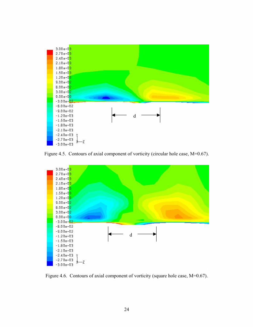
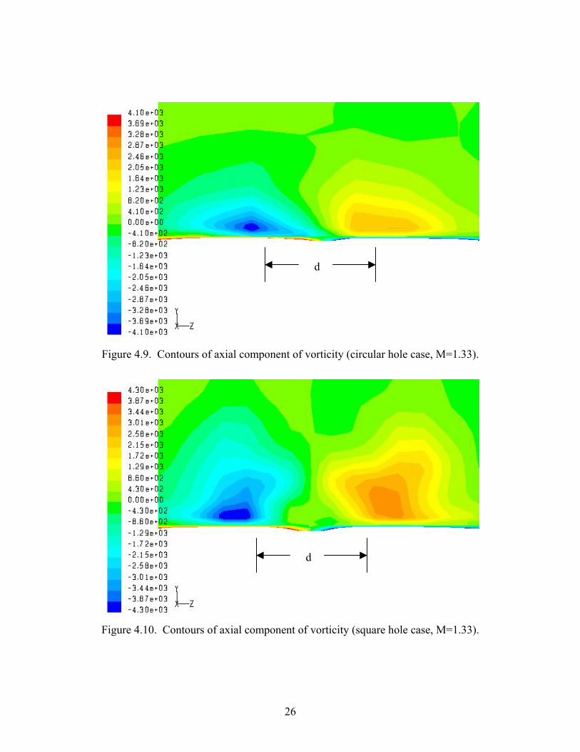
Comparisons of circular and square hole case plots of vorticity contours in a plane at an

axial distance of 2 mm from the leading edge of the hole for blowing ratios of 0.33, 0.5, 0.67,

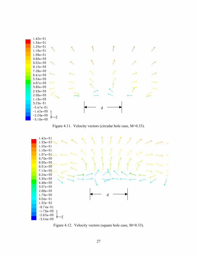
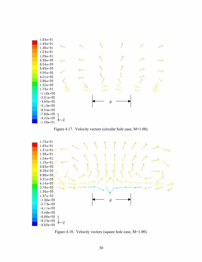
1.0, and 1.33 are made in Figures 4.1-4.10. Comparisons of circular and square hole case plots

of velocity vectors in a plane at an axial distance of 2 mm from the leading edge of the hole for

blowing ratios of 0.33, 0.5, 0.67, 1.0, and 1.33 are made in Figures 4.11-4.20. There is no

significant difference in maximum vorticity magnitude between the two cases (circular and

square), although of course vorticity magnitude does increase with increasing blowing ratio. The

obvious qualitative difference between the two cases at each blowing ratio is the much greater

lateral separation of the vortices in the square-hole case; this can be observed in both the

vorticity contour and velocity vector plots.

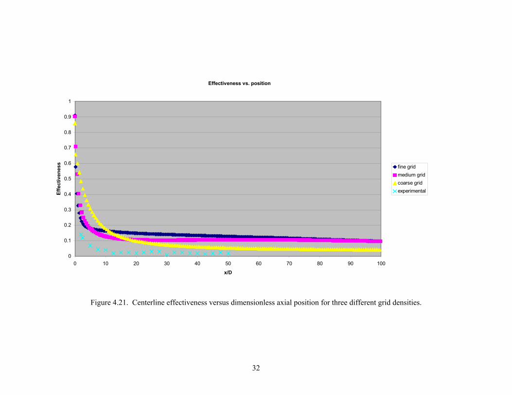
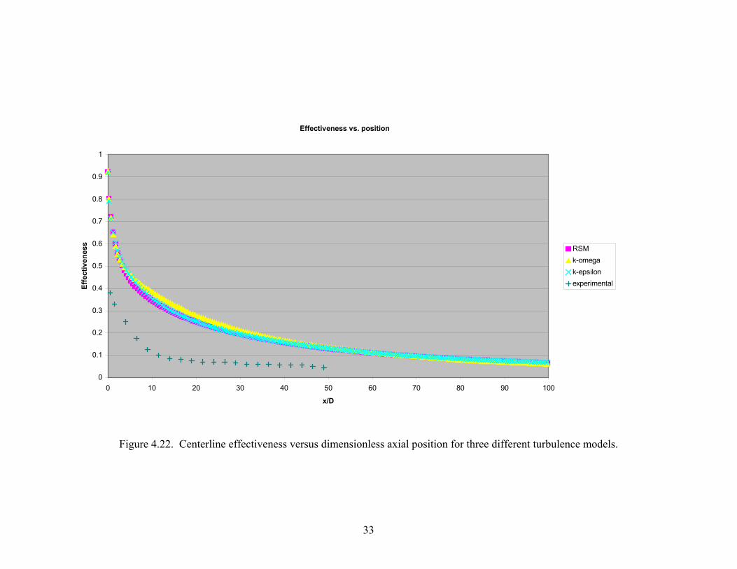
A plot of centerline effectiveness versus dimensionless axial position is shown for three

different grid densities in Figure 4.21, for three different turbulence models (RSM, k-ω, and k-ε)

in Figure 4.22, and for two different wall treatments (wall functions and near-wall treatment) in

Figure 4.23. Following the grid density study, it was thought that the medium grid gave the best

comparison to published experimental results and thus should be used for subsequent

computations. The turbulence model comparison study showed that there was no significant

dependence of results on the turbulence model used; however, it was decided to proceed with

RSM because RSM is the appropriate choice for non-isotropic flows. Finally, the wall treatment

comparison showed that enhanced wall treatment gave the best comparison to published results.

20

This necessitated a change in grid density, since the medium density mesh was not fine enough

for enhanced wall treatment.

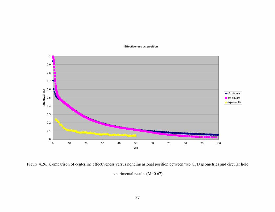
Comparisons of centerline effectiveness versus dimensionless position between the two

CFD geometries and experimental results from Yuen and Martinez-Botas (2003a) for blowing

ratios of 0.33, 0.5, 0.67, 1.0, and 1.33 are shown in Figures 4.24-4.28. This comparison of

computational to experimental data can be compared to a similar comparison by Walters and

Leylek (1997), shown in Figure 4.29. Several trends can be observed in these figures. The

computational results for the circular and square hole cases show that effectiveness is greater for

the square hole immediately downstream of the hole but less for the square hole far downstream

of the hole. It is also observed that the computational results shown in Figures 4.24-4.28 far

over-predict the effectiveness found experimentally; this disagreement was also observed by

Walters and Leylek.

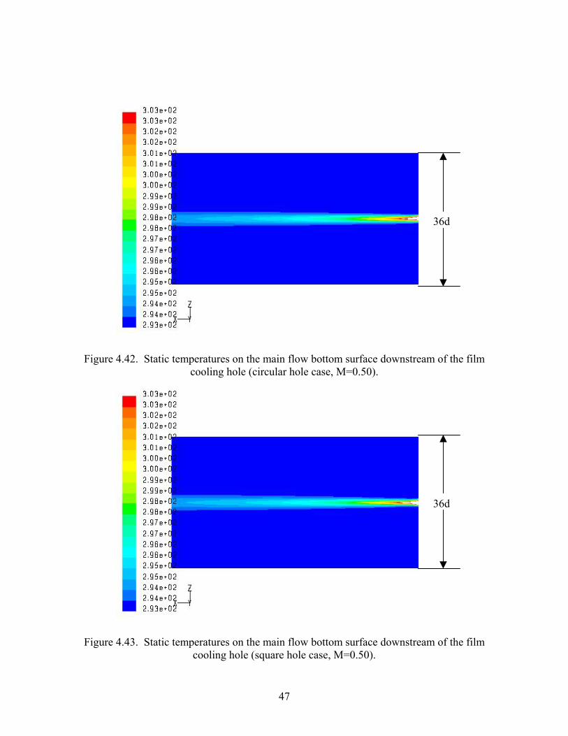
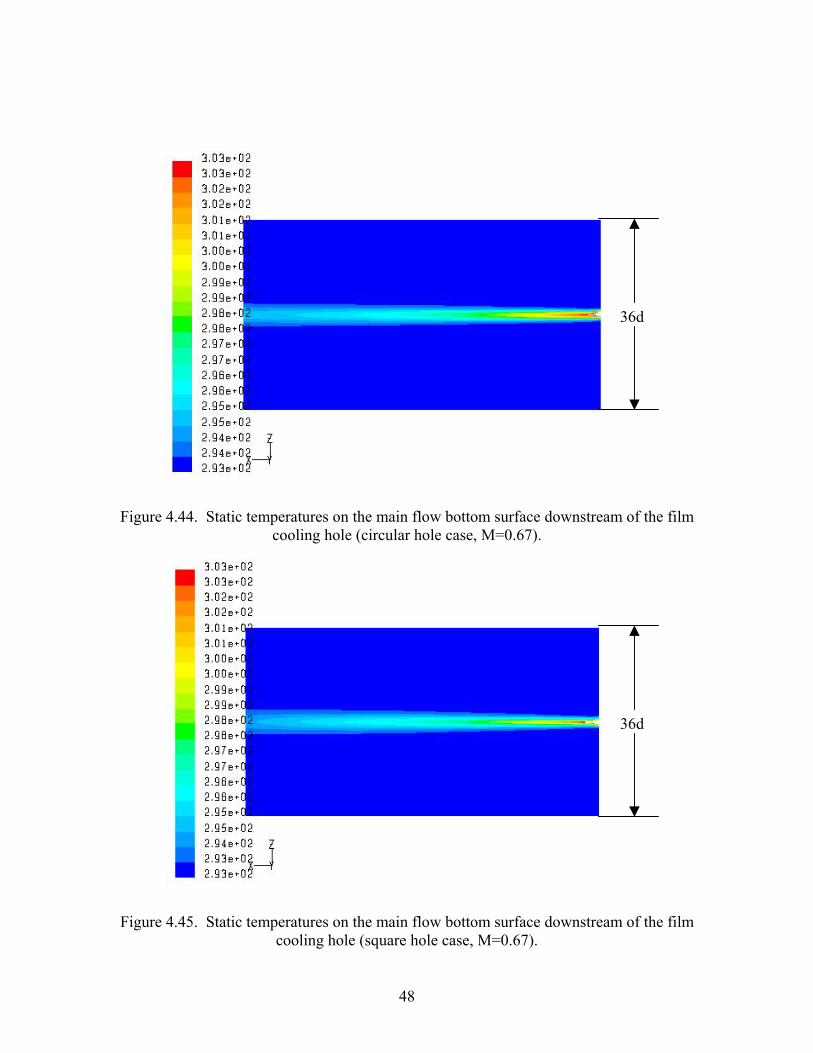
Comparisons of circular and square hole case plots of velocity vectors in a vertical plane

passing through the centerline for blowing ratios of 0.33, 0.5, 0.67, 1.0, and 1.33 are made in

Figures 4.30-4.39. Comparisons of circular and square hole case plots of static temperature on

the bottom main flow surface downstream of the hole for blowing ratios of 0.33, 0.5, 0.67, 1.0,

and 1.33 are made in Figures 4.40-4.49. These figures clearly show that the amount of lateral

spreading of coolant far downstream of the hole is better for square holes, especially at high

blowing ratios. This appears to be the result of the greater lateral separation of vortices in the

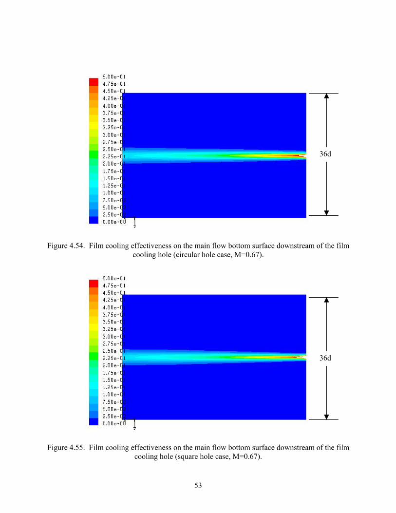
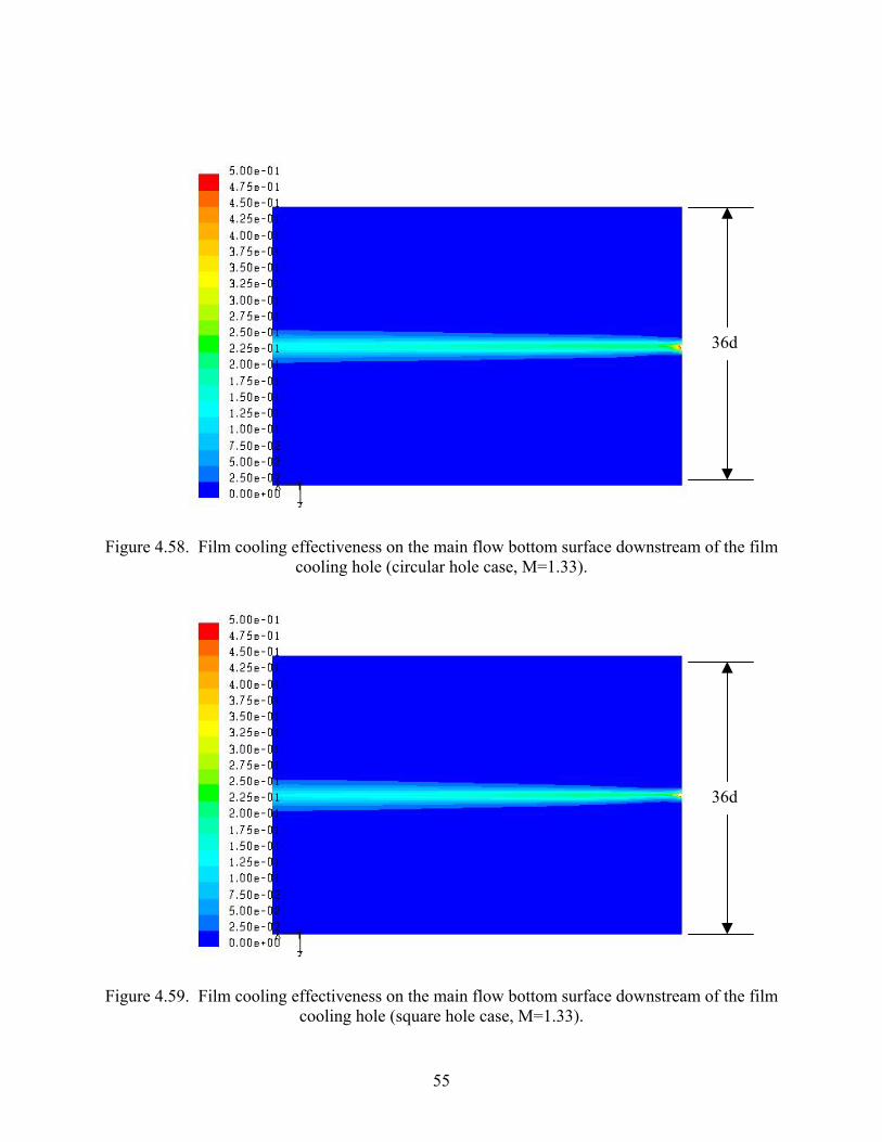
square hole case horseshoe vortex pair. Finally, comparisons of circular and square hole case

plots of effectivness on the bottom main flow surface downstream of the hole for blowing ratios

of 0.33, 0.5, 0.67, 1.0, and 1.33 are made in Figures 4.50-4.59.

21

d

Figure 4.1. Contours of axial component of vorticity (circular hole case, M=0.33).

d

Figure 4.2. Contours of axial component of vorticity (square hole case, M=0.33).

22

d


d


23

d


d


24

d


d


25

d


d


26

d

Figure 4.11. Velocity vectors (circular hole case, M=0.33).

d

Figure 4.12. Velocity vectors (square hole case, M=0.33).

27

d


d


28

d


d


29

d


d


30

d


d


31

Effectiveness vs. position

0

0.1

0.2

0.3

0.4

0.5

0.6

0.7

0.8

0.9

1

0 10 20 30 40 50 60 70 80 90 100

x/D

Effe

ctiv

enes

s fine gridmedium gridcoarse gridexperimental

Figure 4.21. Centerline effectiveness versus dimensionless axial position for three different grid densities.

32


0

0.1

0.2

0.3

0.4

0.5

0.6

0.7

0.8

0.9

1

0 10 20 30 40 50 60 70 80 90 100

x/D

Effe

ctiv

enes

s RSMk-omegak-epsilonexperimental

Figure 4.22. Centerline effectiveness versus dimensionless axial position for three different turbulence models.

33


0

0.1

0.2

0.3

0.4

0.5

0.6

0.7

0.8

0.9

1

0 10 20 30 40 50 60 70 80 90 100

x/D

Effe

ctiv

enes

s

RSM with wall functionsRSM with enhanced wall treatmentexperimental

Figure 4.23. Centerline effectiveness versus dimensionless axial position for two different wall treatments.

34


0

0.1

0.2

0.3

0.4

0.5

0.6

0.7

0.8

0.9

1

0 10 20 30 40 50 60 70 80 90 100

x/D

Effe

ctiv

enes

s

cfd circularcfd squareexp circular

Figure 4.24. Comparison of centerline effectiveness versus nondimensional position between two CFD geometries and circular hole

experimental results (M=0.33).

35


0

0.1

0.2

0.3

0.4

0.5

0.6

0.7

0.8

0.9

1

0 10 20 30 40 50 60 70 80 90 100

x/D

Effe

ctiv

enes

s




36


0

0.1

0.2

0.3

0.4

0.5

0.6

0.7

0.8

0.9

1

0 10 20 30 40 50 60 70 80 90 100

x/D

Effe

ctiv

enes

s




37


0

0.1

0.2

0.3

0.4

0.5

0.6

0.7

0.8

0.9

1

0 10 20 30 40 50 60 70 80 90 100

x/D

Effe

ctiv

enes

s

cfd circular

cfd square

exp circular



38


0

0.1

0.2

0.3

0.4

0.5

0.6

0.7

0.8

0.9

1

0 10 20 30 40 50 60 70 80 90 100

x/D

Effe

ctiv

enes

s




39

Figure 4.29. Comparison of computationally obtained centerline effectiveness data of Walters and Leylek (1997) to published experimentally obtained data.

40



41



42



43



44



45

36d

Figure 4.40. Static temperatures on the main flow bottom surface downstream of the film cooling hole (circular hole case, M=0.33).

36d

Figure 4.41. Static temperatures on the main flow bottom surface downstream of the film cooling hole (square hole case, M=0.33).

46

36d


36d


47

36d


36d


48

36d


36d


49

36d


36d


50

36d

Figure 4.50. Film cooling effectiveness on the main flow bottom surface downstream of the film cooling hole (circular hole case, M=0.33).

36d

Figure 4.51. Film cooling effectiveness on the main flow bottom surface downstream of the film cooling hole (square hole case, M=0.33).

51

36d

Figure 4.52. Film cooling effectivness on the main flow bottom surface downstream of the film cooling hole (circular hole case, M=0.50).

36d


52

36d


36d


53

36d


36d


54

36d


36d


55

CHAPTER 5 CONCLUSIONS AND FUTURE RECOMMENDATIONS

In order to investigate whether or not the distribution of film cooling effectiveness in a

gas turbine can be improved using film cooling holes with simple shapes, a computational study

comparing film cooling effectiveness downstream of a single hole with a square cross section to

film cooling effectiveness downstream of a single hole with a circular cross section was

performed. Since it was thought that any difference in film cooling effectiveness might be the

result of differences in the vortex structures generated within the hole and downstream of the

hole, the kidney vortices immediately downstream of the hole were compared between the two

cases. It was found that the square hole gave greater lateral separation of the kidney vortices

immediately downstream of the hole that resulted in increased film cooling effectiveness

immediately downstream of the hole and improved lateral distribution of coolant far downstream

of the hole.

Before any recommendations can be made to gas turbine manufacturers as a result of the

findings shown in this study, some future work is suggested. To be able to completely resolve

the secondary vortices inside the square hole and to make conclusive qualitative and quantitative

comparisons between the circular and square hole cases, a more thorough grid convergence study

should be carried out; unfortunately, due to the limitations of the computational resources

available, it was not possible to do that for this study. In order to achieve the most valid possible

quantitative results from the computational model, constants in the turbulence model could be

varied until the results of the computational model match those of the experiment. Finally, to

obtain computational results for a cooling hole having a geometry that more realistically

56

represents that of a hole used in an actual turbine, the study could be redone using a hole with a

higher length-to-diameter ratio.

57

LIST OF REFERENCES

Baldauf, S., Schulz, A., and Wittig, S., 2001, “High-Resolution Measurements of Local

Effectiveness From Discrete Hole Film Cooling,” ASME Journal of Turbomachinery,Vol. 123,

pp. 758-765

Brown, A., and Saluja, C.L., 1978, “Film Cooling from a Single Hole and a Row of

Holes of Variable Pitch to Diameter Ratio,” International Journal of Heat and Mass Transfer,

Vol. 22, pp. 525-533.

Cho, H.H., Kang, S.G., Rhee, D.H., 2001, “Heat/Mass Transfer Measurement Within a

Film Cooling Hole of Square and Rectangular Cross Section,” ASME Journal of

Turbomachinery, Vol. 123, pp. 806-814.

Elovic, E., and Koffel, W.K., 1983, “Some Considerations in the Thermal Design of

Turbine Airfoil Cooling Systems,” International Journal of Turbo and Jet-Engines, Vol. 1, pp.

45-65.

Goldstein, R.J., Eckert, E.R.G., Ramsey, J.W., 1968, “Film Cooling With Injection

Through Holes: Adiabatic Wall Temperatures Downstream of a Circular Hole,” ASME Journal

of Engineering for Power, Vol. 90, pp. 384-395.

Goldstein, R.J., 1971, “Film Cooling,” Advances in Heat Transfer, Vol. 7, Academic

Press, New York, pp. 321-371.

Haven, B.A., Yamagata, D.K., Kurosaka, M., Yamawaki, S., and Maya, T., 1997, “Anti-

Kidney Pair of Vortices in Shaped Holes and Their Influence on Film Cooling Effectiveness,”

ASME Paper No. 97-GT-45.

58

Haven, B.A., and Kurosaka, M., 1997, “Kidney and Anti-Kidney Vortices in Crossflow

Jets,” Journal of Fluid Mechanics, Vol. 352, pp. 27-64.

Heidmann, J.D., and Hunter, S.D., 2001, “Coarse Grid Modeling of Turbine Film

Cooling Flows Using Volumetric Source Terms,” ASME Paper No. 2001-GT-0138.

Licu, D.N., Findlay, M.J., Gartshore, I.S., Salcudean, M., 2000, “Transient Heat Transfer

Measurements Using a Single Wide-Band Liquid Crystal Test,” ASME Journal of

Turbomachinery, Vol. 122, pp. 546-552.

Rhee, D.H., Lee, Y.S., Kim, Y.B., and Cho, H.H., 2003, “Film Cooling and Thermal

Field Measurements for Staggered Rows of Rectangular-Shaped Film Cooling Holes,” ASME

Paper No. GT2003-38608, Proceedings of ASME Turbo Expo 2003.

Takahashi, H., Nuntadusit, C., Kimoto, H., Ishida, H., Ukai, T., and Takeishi, K., 2001,

“Characteristics of Various Film Cooling Jets Injected in a Conduit,” Annals New York Academy

of Sciences, pp. 345-352.

Walters, D.K., and Leylek, J.H., 1997, “A Systematic Computational Methodology

Applied to a Three-Dimensional Film-Cooling Flowfield,” ASME Journal of Turbomachinery,

Vol. 119, pp. 777-785.

Walters, D.K., and Leylek, J.H., 2000, “A Detailed Analysis of Film-Cooling Physics:

Part I—Streamwise Injection With Cylindrical Holes,” ASME Journal of Turbomachinery, Vol.

122, pp. 102-112.

Yu, Y., Yen, C.-H., Shih, T.I.-P., Chyu, M.K., Gogineni, S., 2003, “Film Cooling

Effectiveness and Heat Transfer Coefficient Distributions Around Diffusion Shaped Holes,”

ASME Journal of Heat Transfer, Vol. 124, pp. 820-827.

59

Yuen, C.H.N., and Martinez-Botas, R.F., 2003, “Film Cooling Characteristics of a Single

Round Hole at Various Streamwise Angles in a Crossflow: Part I Effectiveness,” International

Journal of Heat and Mass Transfer, Vol. 46, pp. 221-235.

Yuen, C.H.N., and Martinez-Botas, R.F., 2003, “Film Cooling Characteristics of a Single

Round Hole at Various Streamwise Angles in a Crossflow: Part II Heat Transfer Coefficients,”

International Journal of Heat and Mass Transfer, Vol. 46, pp. 237-249.

60

comparison of square-hole and round-hole film cooling: a

Documents