comparison of spectral methods through the adjacency matrix and

Diploma Thesis:

Comparison of Spectral MethodsThrough the Adjacency Matrix and

the Laplacian of a Graph

Philipp Zumstein

submitted 28. February 2005 at ETH Zurich

Prof. Dr. Emo Welzl Dr. Tibor Szabo

Contents

0 Preface 5

1 Preliminaries 71.1 Graph Theory . . . . . . . . . . . . . . . . . . . . . . . . . . . 71.2 Matrix Theory . . . . . . . . . . . . . . . . . . . . . . . . . . 9

1.2.1 Basics about Eigenvalues . . . . . . . . . . . . . . . . . 91.2.2 Symmetric Matrices . . . . . . . . . . . . . . . . . . . 101.2.3 Positive Semidefinite Matrices . . . . . . . . . . . . . . 11

1.3 Asymptotic notations . . . . . . . . . . . . . . . . . . . . . . . 12

2 Spectral graph theory 132.1 Definitions and Basic Facts . . . . . . . . . . . . . . . . . . . . 13

2.1.1 The Adjacency Matrix . . . . . . . . . . . . . . . . . . 132.1.2 The Laplacian . . . . . . . . . . . . . . . . . . . . . . . 162.1.3 The normalized Laplacian . . . . . . . . . . . . . . . . 192.1.4 Relations between the Adjacency and the Laplacian . . 21

2.2 The theory of nonnegative matrices . . . . . . . . . . . . . . . 232.3 Trace of a Matrix . . . . . . . . . . . . . . . . . . . . . . . . . 272.4 Eigenvectors . . . . . . . . . . . . . . . . . . . . . . . . . . . . 322.5 Rayleigh quotient . . . . . . . . . . . . . . . . . . . . . . . . . 362.6 Interlacing . . . . . . . . . . . . . . . . . . . . . . . . . . . . . 39

2.6.1 Interlacing Theorems . . . . . . . . . . . . . . . . . . . 392.6.2 Interlacing for Independent Set . . . . . . . . . . . . . 412.6.3 Interlacing for Hamiltonicity . . . . . . . . . . . . . . . 42

2.7 Gerschgorin’s Theorem . . . . . . . . . . . . . . . . . . . . . . 422.8 Majorization . . . . . . . . . . . . . . . . . . . . . . . . . . . . 442.9 Miscellaneous . . . . . . . . . . . . . . . . . . . . . . . . . . . 45

3 Cauchy-Schwarz and other Inequalities 473.1 Cauchy-Schwarz Inequalitiy . . . . . . . . . . . . . . . . . . . 473.2 An inequality . . . . . . . . . . . . . . . . . . . . . . . . . . . 48

3

3.3 Some Spectral Technique . . . . . . . . . . . . . . . . . . . . . 50

4 Pseudo-random graphs 554.1 Models . . . . . . . . . . . . . . . . . . . . . . . . . . . . . . . 554.2 Basics about Pseudo-random graphs . . . . . . . . . . . . . . 564.3 Edge Connectivity . . . . . . . . . . . . . . . . . . . . . . . . 634.4 Maximum Cut . . . . . . . . . . . . . . . . . . . . . . . . . . . 664.5 Vertex Connectivity . . . . . . . . . . . . . . . . . . . . . . . . 684.6 Independent Set . . . . . . . . . . . . . . . . . . . . . . . . . . 704.7 Colorability . . . . . . . . . . . . . . . . . . . . . . . . . . . . 724.8 Hamiltonicity . . . . . . . . . . . . . . . . . . . . . . . . . . . 734.9 Small subgraphs . . . . . . . . . . . . . . . . . . . . . . . . . . 73

5 Turan’s Theorem 835.1 Classical Turan’s Theorem . . . . . . . . . . . . . . . . . . . . 835.2 Generalization to (n, d, λ)-graphs . . . . . . . . . . . . . . . . 855.3 Comments about Chung’s paper . . . . . . . . . . . . . . . . . 86

5.3.1 Lemmas . . . . . . . . . . . . . . . . . . . . . . . . . . 875.3.2 Negligence of the λ2-term . . . . . . . . . . . . . . . . 89

Appendix 91List of Definitions . . . . . . . . . . . . . . . . . . . . . . . . . . . . 91List of Theorems . . . . . . . . . . . . . . . . . . . . . . . . . . . . 92Maple-Code . . . . . . . . . . . . . . . . . . . . . . . . . . . . . . . 93

Bibliography 96

4

Chapter 0

Preface

Graph theory and linear algebra are two beautiful fields of mathematics andspectral graph theory lies in their intersection. More exactly, spectral graphtheory deals with the properties of a graph in relationship to the eigenvaluesand eigenvectors of some associated matrix.

First, in chapter 1 we will collect the preliminaries of graph and matrix the-ory and introduce the usual asymptotic notations. Then in chapter 2 wewill define the different kinds of matrices of a graph, namely the adjacencymatrix, the Laplacian and the normalized Laplacian. After some basic factswe will describe different methods that exist in spectral graph theory andgive some applications.

In chapter 3 we will state the Cauchy-Schwarz and other inequalities. Wewill also discover spectral techniques using the Cauchy-Schwarz Inequality.After that we are ready to discuss pseudo-random graphs.

Pseudo-random graphs are graphs which behave like random graphs. Inchapter 4 we will define the concept of pseudo-random graphs via eigenval-ues. There are two approaches to do that. One considers the spectrum of theadjacency matrix and the other the spectrum of the normalized Laplacian.The first approach is mostly easier to apply but only adaptable for d-regulargraphs. We will then generalize some statements of the survey paper aboutpseudo-random graphs by Krivelevitch and Sudakov [18] for the normalizedLaplacian.

Finally, in chapter 5 we will discuss Turan’s Theorem and some attempts toextend this theorem for pseudo-random graphs.

5

Acknowledgement. I would like to thank my advisor Dr. Tibor Szabo andProf. Emo Welzl. Also, I would like to thank everyone who read parts ofthis thesis and made suggestions to its improvement.

6

Chapter 1

Preliminaries

1.1 Graph Theory

Most of the material of graph theory is taken from West [30] and Jukna [15].

A (simple) graph is a pair G = (V,E) consisting of a set V , whose elementsare called vertices, and a family E of 2-element subsets of V , whose membersare called edges. A directed graph is pair G = (V,E) consisting of a set V(vertices) and a set E (edges) of ordered pairs of V . The first vertex of theordered pair is the tail of the edge and the second is the head ; together theyare called endpoints. In the following the concept of directed graph is rarelyneeded. We continue now the discussion about (simple) graphs.

A subgraph of G = (V,E) is a pair H = (W,F ) such that W ⊆ V, F ⊆ E.An induced subgraph of G = (V,E) is a set of vertices W and all edges fromG which have both endpoints in W ; the induced subgraph of G spanned bythe vertices is denoted by G[W ].

A vertex v is incident with an edge e if v ∈ e. Two vertices u, v of G areadjacent, or neighbors, if u, v is an edge of G. We denote the set of allneighbors of u by N(u). We will write u ∼ v if u and v are adjacent. Avertex which has no neighbors is called isolated. The number du of neighborsof a vertex u is its degree. A graph is called d-regular if all degrees are d.The maximum degree of a graph G is denoted by ∆(G) (or simply ∆) andthe minimum degree by δ(G) (or simply δ).

7

Lemma 1.1 Let G = (V,E) be a graph. Then

∑

v∈V

dv = 2|E|.

A walk of length k in G is a sequence v0, e1, v1, ..., ek, vk of vertices and edgessuch that ei = vi−1, vi for all i. A walk without repeated vertices is a path.A cycle is a closed path, i.e. a path with an edge from the first vertex tothe last one. A component in a graph is a maximal set of vertices such thatthere is a path between any two of them. A graph is connected if it consistsof one component. Mutatis mutandis: A directed graph is strongly connectedif there exists a directed path between any two of the vertices.

A Hamiltonian cycle of a graph G = (V,E) is cycle of length n = |V |, i.e.the cycle goes through all vertices once. A graph is called Hamiltonian if itconsists a Hamiltonian cycle.

An independent set in a graph is a set of vertices with no edges betweenthem. The greatest integer r such that G contains an independent set of sizer is the independence number of G, and is denoted by α(G).

A complete graph or clique is a graph in which every pair of vertices is ad-jacent. The complete graph on n vertices is denoted by Kn. A graph isbipartite if its vertex set can be partitioned into two independent sets. Thecomplete bipartite graph is denoted by Kn,m where n is the size of one partand m is the size of the other part. The star Sn = K1,n−1 is the completebipartite graph on n vertices in which one part has size 1. More generally,a graph is r-partite if its vertex set can be partitioned into r independent sets.

Lemma 1.2 G is bipartite ⇐⇒ G contains no odd cycle.

Let G be a graph and S a subset of vertices. G − S is the graph obtainedfrom G by deleting the vertices S (and all edges incident to some vertex fromS). The connectivity of G, written κ(G), is the minimum size of a vertex setS such that G − S is disconnected. The connectivity of the complete graphKn is defined as n−1. A graph G is k-connected if its connectivity is at least k

A disconnecting set of edges is a set F ⊆ E(G) such that G−F has more thanone component. A graph is k-edge-connected if every disconnecting set hasat least k edges. The edge-connectivity of G, written κ′(G), is the minimumsize of a disconnecting set.

8

Theorem 1.3 (Whitney) If G is a simple graph, then

κ(G) ≤ κ′(G) ≤ δ(G).

A proper coloring of G is an assignment of colors to each vertex so that adja-cent vertices receive different colors. The minimum number of colors requiredfor that is the chromatic number χ(G) of G.

A perfect matching M in a graph G is a set of disjoint edges such that everyvertex is incident to (exactly) one edge from M . Thus, a necessary conditionfor the existence of a perfect matching is that there is an even number ofvertices.

Theorem 1.4 (Tutte’s 1-Factor Theorem) A graph G has a perfect match-ing if and only if the number of odd components of G − S is at most as bigas |S| for every subset S of vertices.

1.2 Matrix Theory

We assume that the reader is familiar with the concepts of a matrix andvector. One should also be acquainted with the operations on matrices andvectors, such as addition, multiplication, transposition (denoted by T ), trace(denoted by tr(·)), inner product and determinant. Here we will only repeatsome facts about the eigenvalues of a matrix. For a more detailed discussionwe refer to the book “Matrix analysis” by Johnson and Horn [26].

We consider m × n matrices over the real numbers. We are mostly lookingat square matrices, i.e. m = n. The vectors v, w are orthogonal (denoted byv ⊥ w) if their inner product vanishes, i.e. vT w = 0.

1.2.1 Basics about Eigenvalues

Let A be a n × n-matrix. λ ∈ C is called an eigenvalue of A if there existsa (complex) vector v 6= 0 such that Av = λv. This vector v is called aneigenvector of A associated with the eigenvalue λ. The set of all eigenvaluesof A is called the spectrum of A, denoted by spec(A).

Lemma 1.5 Let p(·) be a given polynomial. If λ is an eigenvalue of A, whilex is an associated eigenvector, then p(λ) is an eigenvalue of the matrix p(A)and x is an eigenvector of p(A) associated with p(λ).

9

The characteristic polynomial of A is defined by

χA(t) := det(tI − A).

Facts: The roots of the characteristic polynomial χA are exactly the eigen-values of A. By the Fundamental Theorem of Algebra we know that everypolynomial with degree n has exactly n complex roots (counted with multi-plicities). So every matrix has n (complex) eigenvalues (counted with multi-plicities).

Lemma 1.6 Let A be a n × n-matrix with eigenvalues λ1, ..., λn. Then

tr(A) =n∑

i=1

λi.

1.2.2 Symmetric Matrices

A square matrix A over the real numbers is symmetric if AT = A, i.e. theith column of A is equal to the ith row of A. (For complex matrices there isthe corresponding concept of Hermitian, which we will not use further.)

Lemma 1.7 Let A be a symmetric real matrix. Suppose v and w are eigen-vectors of A associated with the eigenvalues λ and µ respectively. If λ 6= µthen v ⊥ w, i.e. v and w are orthogonal.

Theorem 1.8 (Spectral Theorem) Let A be a n× n symmetric real ma-trix. Then there are n pairwise orthogonal (real) eigenvectors vi of A associ-ated with real eigenvalues of A.

We can order the eigenvalues of a symmetric matrix because all eigenvaluesare real by the Spectral Theorem 1.8. We will denote the eigenvalues of asymmetric matrix A by λ1(A) ≤ . . . ≤ λn(A). Some of these eigenvaluescan be equal; we say that those eigenvalues have multiplicity greater than 1.Thus we will write the spectrum of A also in the form λ

[m1]1 , . . . , λ

[mk]k , where

λi is an eigenvalue with multiplicity mi.

The eigenvalues of symmetric matrices can be expressed as an extremal valueof some term, i.e. they are the maximum, minimum of some function:

10

Theorem 1.9 (Rayleigh-Ritz) Let A be an n× n real symmetric matrix,and let λ1 ≤ λ2 ≤ ... ≤ λn be the eigenvalues of A. Then

λn = maxx6=0

xT Ax

xT x= max

xT x=1xT Ax,

λ1 = minx6=0

xT Ax

xT x= min

xT x=1xT Ax.

The expression R(A; x) := xT Ax/xT x is called the Rayleigh quotient. Thetheorem above gives us an extremal characterization of the largest and small-est eigenvalue of a symmetric matrix. There exists a more general theorem:

Lemma 1.10 Let A be a n × n real symmetric matrix with eigenvaluesλ1 ≤ λ2 ≤ ... ≤ λn and corresponding eigenvectors v1, v2, ..., vn such thatthey are pairwise orthogonal. Then for all integers 1 ≤ k ≤ n − 1:

λk+1 = minx6=0

x⊥v1,...,vk

xT Ax

xT x= min

xT x=1x⊥v1,...,vk

xT Ax,

λn−k = maxx6=0

x⊥vn,...,vn−k+1

xT Ax

xT x= max

xT x=1x⊥vn,...,vn−k+1

xT Ax.

Eigenvectors must be known explicitly to apply this theorem. If one doesnot known the eigenvectors, one can use the following theorem:

Theorem 1.11 (Courant-Fischer) Let A be an n×n real symmetric ma-trix with eigenvalues λ1 ≤ λ2 ≤ ... ≤ λn. Then for a given integer k suchthat 1 ≤ k ≤ n:

λk = minw1,...,wn−k∈Rn

maxx∈R

n−0x⊥w1,...,wn−k

xT Ax

xT x;

λk = maxw1,...,wk−1∈Rn

minx∈R

n−0x⊥w1,...,wk−1

xT Ax

xT x.

1.2.3 Positive Semidefinite Matrices

An n × n symmetric matrix is said to be positive semidefinite if xT Ax ≥ 0for all x ∈ R

n

Theorem 1.12 (positive semidefinite matrices) Let A be a real sym-metric matrix. The following conditions are equivalent:

• The matrix A is positive semidefinite.

• All eigenvalues of A are nonnegative.

11

1.3 Asymptotic notations

Some of the results are asymptotic, and we use the standard asymptotic no-tation: Let f and g be two functions over R. We write f = O(g) if there areconstants C > 0, n0 ∈ R such that |f(n)| ≤ C|g(n)| for all n ≥ n0. We writef = o(g) or equivalently f g if f/g → 0 as n → ∞. We write f = Ω(g) ifg = O(f), i.e. there are constants C > 0, n0 ∈ R such that |f(n)| ≥ C|g(n)|for all n ≥ n0. Finally we write f = Θ(g) if f = O(g) and f = Ω(g).

The variable n will most of the time be the number of vertices of a graph.So we will look at families of graphs with more and more vertices and makethere some asymptotic assertions.

12

Chapter 2

Spectral graph theory

In the following chapter we will first define the different kinds of matricesof a graph, namely the adjacency matrix, the Laplacian and the normalizedLaplacian. These definitions may be found in section 2.1 where we will alsostate and prove some basic facts that follow naturally. Sections 2.2 till 2.8will deal with the different methods that exist in spectral graph theory. Wewill describe these methods, give some applications and show for which kindsof matrices one may use a specific method. In the last section we will mentionsome other stuff about spectral graph theory.

2.1 Definitions and Basic Facts

In the following we will often consider a graph on n vertices. To simplifynotations, we will suggested that these vertices are 1, 2, ..., n.

2.1.1 The Adjacency Matrix

Definiton 2.1 (adjacency matrix) Let G be a simple graph on n vertices.The adjacency matrix A(G) is a matrix of dimension n× n. The ij-th entryof A(G) is 1 if the vertices i and j are connected by an edge, otherwise it is0, i.e.

A(G)ij :=

1, if i ∼ j;0, otherwise.

The adjacency matrix of a graph contains the same information as the graphitself. So it is a possibility to store a graph in a computer.

13

([4], p.164f): Two graphs X and Y are isomorphic if there is a bijection,φ say, from V (X) to V (Y ) such that x ∼ y in X if and only if φ(x) ∼ φ(y)in Y . We say that φ is an isomorphism from X to Y . Thus, an isomorphismcan be viewed as an relabeling of the vertices. It is normally appropriateto treat isomorphic graphs as if they were equal. The adjacency matrixof two isomorphic graphs X,Y is in general not the same, but there is apermutation matrix Φ such that ΦT A(X)Φ = A(Y ). Since permutationmatrices are orthogonal, ΦT = Φ−1, the characteristic polynomial of A(X)and A(Y ) is the same, i.e.

χA(Y )(t) = det(tI − A(Y )) = det(tΦ−1IΦ − Φ−1A(X)Φ)

= det(Φ−1) det(tI − A(X)) det(Φ) = χA(X)(t).

Thus, also the eigenvalues of the adjacency matrix are indifferent under iso-morphic transformations.

Definiton 2.2 (adjacency eigenvalues) The eigenvalues of A(G) are calledthe adjacency eigenvalues of G. The set of all the adjacency eigenvalues arecalled the (adjacency) spectrum of the graph G.

Example 2.3 We look at the graph G = K3:

adjacency matrix:

0 1 11 0 11 1 0

characteristic polynomial:

χ(x) = x3 − 3x − 2

adjacency eigenvalues:

2, 1, 1

We notice that A(G) is a symmetric real-valued matrix. So we know from theSpectral Theorem 1.8 that all the adjacency eigenvalues are real and we haven such eigenvalues (counted with multiplicity). So we can assume that theeigenvalues of a graph G are ordered λ1 ≤ λ2 ≤ . . . ≤ λn. We note that thisis an abbreviated notation for the adjacency eigenvalues, i.e. λi = λi(A(G)).

Next, we determine the range of the adjacency eigenvalues.

Lemma 2.4 ([3] p.51, [29] p.6) Let G be a graph on n vertices.i) The maximum eigenvalue of G lies between the average and the maximumdegree of G, i.e.

d ≤ λn ≤ ∆.

14

ii) The range of all the eigenvalues of a graph is

−∆ ≤ λ1 ≤ λ2 ≤ . . . ≤ λn ≤ ∆.

Proof: i) We will show that the Rayleigh quotient for some special vector isgreater than d. This suffices to get the first inequality, because the maximumof the Rayleigh quotient is λn (cf. Rayleigh-Ritz Theorem 1.9). The otherinequality in i) follows from the second point.Set x = (1, 1, ..., 1)T . The Rayleigh quotient for this vector equals:

R(A; x) =xT Ax

xT x=

∑ni=1

∑nj=1 xiAijxj

∑ni=1 x2

i

=

∑ni=1

∑

j:j∼i 1

n=

∑ni=1 di

n= d.

(1)ii) We have to show that the absolute value of every eigenvalue is less thanor equal to the maximum degree. Let u be an eigenvector corresponding tothe eigenvalue λ, and let uj denote the entry with the largest absolute value.We have

|λ||uj| = |λuj| = |(Au)j| =

∣∣∣∣∣

∑

i∼j

ui

∣∣∣∣∣≤∑

i∼j

|ui| ≤ dj|uj| ≤ ∆|uj|.

Thus we have |λ| ≤ ∆ as required.

Corollary 2.5 ([3], p.14) Let G be a d-regular graph. Then:i) λn = d is the greatest eigenvalue with eigenvector (1, 1, ..., 1)T .ii) For any eigenvalue λi of G, we have |λi| ≤ d.

Proof: We note that the average degree in a d-regular graph is d and alsothe maximum degree is d. So the greatest eigenvalue λn has to be d byLemma 2.4 part i). Moreover, d is an adjacency eigenvalue with associatedeigenvector (1, . . . , 1)T because every row of A(G) contains exactly d ones.The second part follows immediately by Lemma 2.4 part ii).

Remark 2.6 Two graphs which have the same spectrum are called iso-spectra. But the spectra of a graph G does not characterize the graphuniquely. There are non-isomorphic graphs with the same spectra. Lookfor example at the following two graphs:

15

0 1 0 1 01 0 1 0 00 1 0 1 01 0 1 0 00 0 0 0 0

0 0 0 0 10 0 0 0 10 0 0 0 10 0 0 0 11 1 1 1 0

The characteristic polynomial of both of this matrices is equal to

χ(x) = x5 − 4x3

So the adjacency eigenvalues of these two graphs are 0 with multiplicity 3, 2and −2, i.e.

spec = 0[3], 2,−2

We notice that the graph on the left is disconnected while the graph onthe right is connected. So this pair of iso-spectra graphs tells us that theconnectivity (in general) is not deducible from the adjacency spectrum.

2.1.2 The Laplacian

Definiton 2.7 (Laplacian) Let G be a graph. We denote the diagonalmatrix with the degrees as diagonal elements by D(G). The Laplacian matrixor Laplacian L(G) is the difference between D(G) and the adjacency matrixA(G), i.e.

L(G)ij :=

di, if i = j;−1, if i ∼ j;0, otherwise.

There is another view of the Laplacian matrix. We can think of the Laplacianas the sum of some matrices L(u, v) which look like the expansion of theLaplacian of an edge, i.e.

16

L(u, v) :=

. . . . ..

1 · · · −1...

...−1 · · · −1

. .. . . .

where the diagonal elements corresponding to u and v are 1, the (u, v) and(v, u) entries are -1 and the rest is fill up with 0.

Lemma 2.8 ([27]) The Laplacian matrix is equal to the following sum:

L(G) =∑

u,v∈E(G)

L(u, v)

Proof: First, we look at the diagonal elements:

∑

u,v∈E(G)

L(u, v)

ii

=∑

u,v∈E(G)

L(u, v)ii = |N(i)| = di = L(G)ii.

The non-diagonal elements are −1 if there is an edge and 0 otherwise. Thisholds for the Laplacian and for the sum of these matrices.

Lemma 2.9 The Laplacian matrix is positive semidefinite, i.e. xT L(G)x ≥0 for all vectors x.

Proof: Let x be any vector. First, we check that the matrix L(u, v) ispositive semidefinite:

xT L(u, v)x = x2u + x2

v − 2xuxv = (xu − xv)2 ≥ 0.

Now, we will look at the Laplacian matrix:

xT L(G)x = xT

∑

u,v∈E(G)

L(u, v)

x =∑

u,v∈E(G)

xT L(u, v)x

=∑

u,v∈E(G)

(xu − xv)2 ≥ 0. (2)

17

Definiton 2.10 (Laplacian eigenvalues) The eigenvalues of L(G) are calledthe Laplacian eigenvalues. The set of all the Laplacian eigenvalues are calledthe (Laplacian) spectrum of the graph G.


Laplacian matrix:

2 −1 −1−1 2 −1−1 −1 2


χ(x) = x3 − 6x2 + 9x

Laplacian eigenvalues:

0, 3, 3

The vector v = (1, 1, ..., 1)T is always an eigenvector of the eigenvalue 0.We know that all the Laplacian eigenvalues are nonnegative because theLaplacian is positive semidefinite. We will bound the Laplacian eigenvaluesfrom above in the next lemma.

Lemma 2.12 ([27]) Let G be a graph on n vertices with Laplacian eigen-values λ1 = 0 ≤ λ2 ≤ ... ≤ λn and maximum degree ∆. Then

0 ≤ λi ≤ 2∆.

Andλn ≥ ∆.

Proof: All eigenvalues are nonnegative by Theorem 1.12 and Lemma 2.9.

Let u be an eigenvector corresponding to the eigenvalue λ, and let uj denotethe entry with the largest absolute value. We have

|λ||uj| = |λuj| =

∣∣∣∣∣djuj −

∑

i∼j

ui

∣∣∣∣∣≤ dj|uj| +

∑

i∼j

|ui| ≤ 2dj|uj| ≤ 2∆|uj|.

Thus, we have |λ| ≤ 2∆ as required.

Let j be the vertex with maximal degree, i.e. dj = ∆. We define thecharacteristic vector x:

xi :=

1, if i = j;0, otherwise.

18

Now, the desired inequality follows:

λn(Thm. 1.9)

= maxx6=0

xT x

xT x≥ xT Lx

xT x

(2)=

∑

u,v∈E(xu − xv)2

1= ∆.

2.1.3 The normalized Laplacian

The normalized Laplacian matrix is the Laplacian matrix with a normaliza-tion of the degree matrix. This normalization will force the eigenvalues tobe in the interval [0, 2].

Suppose G is a graph with no isolated vertices. Then the diagonal matricesD1/2 and D−1/2 are uniquely determined by taking the square root of eachentry and the (−1/2)-power of each entry, respectively. If G has an isolatedvertex i then D1/2 and D−1/2 are not uniquely determined because di = 0.

Definiton 2.13 (normalized Laplacian) Let G be a graph without iso-lated vertices. The normalized Laplacian of G is the matrix

L(G) = D−1/2LD−1/2

i.e.

L(G)ij :=

1, if i = j and i 6= 0;− 1√

didj, if i ∼ j;

0, otherwise.

Remark 2.14 i) The following equality holds

L(G) = D−1/2LD−1/2 = I − D−1/2AD−1/2. (3)

ii) Let us for a moment look at a graph with isolated vertices. Now we definethe matrix D−1/2 as the diagonal matrix with entries 1√

djif dj 6= 0 and 0

otherwise. We can now extend the definition of the normalized Laplacianto graphs with isolalted vertices, i.e. L(G) = D−1/2LD−1/2. However, theproblem is now that equation (3) is not true in general. To see this, we let ibe an isolated vertex. Then the ith row and ith column of D−1/2 consistingonly zeros. So

L(G)ii = (D−1/2LD−1/2)ii = 0

but(I − D−1/2AD−1/2)ii = 1.

19

This problem occurs in Chung’s book [6] as an oversight. To avoid this dif-ficulty we make the following convention.

Convention: Every graph in the following has no isolated vertices.

Definiton 2.15 (normalized Laplacian eigenvalues) The eigenvalues ofthe normalized Laplacian are called the normalized Laplacian eigenvalues.

Since L is symmetric, its eigenvalues are real and we can assume that theyare ordered, i.e. λ1 ≤ λ2 ≤ . . . ≤ λn. (But we do not know yet if they arenegative or not.) (Note that we count the eigenvalues from 1 to n and notfrom 0 to n − 1 as Chung does.)


norm. Laplacian matrix:

1 −12

−12

−12

1 −12

−12

−12

1


χ(x) = x3 − 3x2 +9

4x

norm. Laplacian eigenval.:

0,3

2,3

2

The vector D1/21 = (√

d1, . . . ,√

dn)T is in general an eigenvector to theeigenvalue 0:

L · D1/21 = D−1/2LD−1/2 · D1/21 = D−1/2L1 = 0.

To get general bounds for the eigenvalues we look at the Rayleigh quotient.Let x be any real vector and y = D(G)−1/2x.

xTLx

xT x=

xT D−1/2LD−1/2x

(D1/2D−1/2x)T (D1/2D−1/2x)=

yT Ly

(D1/2y)T (D1/2y).

Here we have used some tiny facts about linear algebra: Diagonal matricesare symmetric, i.e. (D−1/2)T = D−1/2; matrix multiplication is associativeand (Mz)T = zT MT . Now, we continue the calculation

R(L; x) =xTLx

xT x

(2)=

∑

u,v∈E(yu − yv)2

∑

u∈V duy2u

(4)

Lemma 2.17 The normalized Laplacian L is positive semidefinite.

20

Proof: The Rayleigh quotient is always nonnegative by (4). Then alsoxTLx ≥ 0 for all x, i.e. L is positive semidefinite.

Lemma 2.18 ([6], p.6) Let G be a graph on n vertices with normalizedLaplacian eigenvalues λ1 = 0 ≤ λ2 ≤ ... ≤ λn. Then

0 ≤ λi ≤ 2

Andλn ≥ n

n − 1

Proof: All the eigenvalues are nonnegative by Lemma 2.17 and Theorem1.12. We have seen before that 0 is an eigenvalue with eigenvector D1/21. Forthe upper bound on the eigenvalues we are looking at the Rayleigh quotientas it was derived in (4) and then use Lemma 1.11:

∑

i∼j(xi − xj)2

∑

i dix2i

≤∑

i∼j 2x2i + 2x2

j∑

i dix2i

=2∑

i dix2i

∑

i dix2i

≤ 2.

The trace of the normalized Laplacian is equal to n. Thus, by Lemma 1.6also the sum of all eigenvalues has to be n. The desired inequality followsfrom the following calculation:

n =n∑

i=1

λi = 0 +n∑

i=2

λi ≤ (n − 1)λn.

2.1.4 Relations between the Adjacency and the Lapla-cian

For all three kinds of eigenvalues we know that the spectrum of G is theunion of the spectra of the components of G. This will let us assume in sometheorems without loss of generality (w.l.o.g.) that G is connected.

Lemma 2.19 Let G be a graph with components V1, ..., Vk. Then

spec(A(G)) =k⋃

i=1

spec(A(G[Vi])),

spec(L(G)) =k⋃

i=1

spec(L(G[Vi])),

spec(L(G)) =k⋃

i=1

spec(L(G[Vi])),

where G[Vi] denotes the induced subgraph of G on the vertices Vi.

21

Proof: After a relabeling of the vertices the three matrices A(G), L(G) andL(G) are block matrices with nonzero blocks in the diagonal and all otherblocks are zero-blocks. The non-zero blocks are corresponding to the associ-ated matrices of one of the components of G. By a straightforward calculationone can see that the spectrum of such a (diagonal) block matrix is the unionof the spectra of its blocks.

We will list the three different kinds of eigenvalues in the following table.

matrix eigenvaluesadjacency A −∆ ≤ λi(A)) ≤ ∆Laplacian L = D − A 0 ≤ λi(L) ≤ 2∆normalized Laplacian L = D−1/2LD−1/2 0 ≤ λi(L) ≤ 2

We have now defined three different matrices and three different types ofeigenvalues. There are relations among them. The simplest case is when welook at d-regular graphs. Then the knowledge of any of the three spectrawould provide us the others via linear functions.

Theorem 2.20 (Relations for d-regular graphs) Let G be a d-regulargraph on n vertices. Then

λi(L(G)) = d − λn−i+1(A(G)),

λi(L(G)) = λi(L(G))/d,

λi(I − L(G)) = λi(A(G))/d.

Proof: The degree matrix D(G) is equal to the d-multiple of the identitymatrix. So every eigenvector of the adjacency matrix is an eigenvector of theLaplacian (and also of the normalized Laplacian). The indices are shiftedbecause we have to preserve the order.

Lemma 2.21 Let G be a graph on n vertices with largest degree ∆, adja-cency matrix A, Laplacian L and normalized Laplacian L. Then

∆ − λn(A) ≤ λn(L) ≤ ∆ − λ1(A).

λi(L)δ ≤ λi(L) ≤ λi(L)∆.

Proof: We look at the Rayleigh quotient:

R(L; x) =xT Lx

xT x=

xT Dx

xT x− xT Ax

xT x= R(D; x) − R(A; x).

22

Then we conclude

λn = maxx6=0

R(L; x) ≤ maxx6=0

R(D; x) − minx6=0

R(A; x) = ∆ − λ1(A).

Let x 6= 0 be the eigenvector of D associated with the eigenvalue ∆. Then

λn(L) = maxx6=0

R(L; x) ≥ R(L; x) = R(D; x) − R(A; x) ≥ ∆ − λn(A).

For the second line let us first have a look at the Rayleigh quotient:

R(L; D−1/2x)(4)=

∑

i∼j(xi − xj)2

∑

i dix2i

≥∑

i∼j(xi − xj)2

∆∑

i x2i

(2)=

R(L; x)

∆.

Now, we use the characterization of the eigenvalues given by the Courant-Fisher Theorem.

λk(L) = minw1,...,wn−k∈Rn

maxx∈R

n−0x⊥w1,...,wn−k

R(L; x)

≤ ∆ minw1,...,wn−k∈Rn

maxx∈R

n−0x⊥w1,...,wn−k

R(L; D−1/2x).

We note that:x ⊥ w, x 6= 0 ⇐⇒ x′ ⊥ w′, x′ 6= 0

where x′ = D−1/2x and w′ = D1/2w. Also we know that D1/2 is invertible.So we can continue

λk(L) ≤ ∆ minw′

1,...,w′

n−k∈Rnmax

x′∈Rn−0

x′⊥w′

1,...,w′

n−k

R(L; x′) = ∆λk(L).

In the same way we get λk(L) ≥ δλk(L).

2.2 The theory of nonnegative matrices

Definiton 2.22 (nonnegative, positive matrices) A matrix M is callednonnegative, if all elements are nonnegative. A matrix M is called positive,if all elements are positive.

The adjacency matrix is a nonnegative matrix but it is not positive becausethe diagonal entries are zero. Perron’s classical Theorem (see e.g. Gant-macher [11], p.398, Satz 1) deals with positive matrices. Thus we cannotapply this theorem to the adjacency matrix. There is a generalization of thistheorem which is called Frobenius’s Theorem. It deals with indecomposable(=unzerlegbaren) matrices:

23

Definiton 2.23 (incomposable/decomposable) ([11], p. 395f) A ma-trix M is called decomposable if it has (up to a permutation of the rows andcolumns) the following form

M =

(B 0C D

)

where B and D are square matrices. Otherwise the matrix M is calledindecomposable.

The meaning of this definition is the following: We associate a directedgraph GM to the matrix M such that there is a directed edge from i toj iff Mij > 0. Clearly, the matrix M is indecomposable iff the graph GM isstrongly connected. We note that a symmetric matrix M is indecomposableiff the associated graph GM is connected.

Example 2.24 Look at the following matrix M and the associated directedgraph GM :

1 1 01 0 01 1 1

1

3

2

The matrix M is decomposable because of the the decomposition shownon the left. The graph GM is not strongly connected, because there is no(directed) path from 1 to 3.

Theorem 2.25 (Perron-Frobenius) Suppose M is a real nonnegative in-decomposable matrix. Then:

1. There exists a positive real simple eigenvalue of M and an associatedeigenvector whose entries are all positive. Let λPF be such an eigen-value.

24

2. All eigenvalues λ of M satisfy |λ| ≤ λPF , i.e. λPF is the largest eigen-value (in absolute value). In particular λPF is unique.

3. If θ is an eigenvalue of M and |θ| = λPF , then θ/λPF is an mth root ofunity and e2πir/mλPF is an eigenvalue of M for all r.

Remark 2.26 i) A simple eigenvalue is an eigenvalue with multiplicity 1.

ii) The eigenvalue λPF is called the Perron-Frobenius eigenvalue of M .

iii) Let M be some real nonnegative symmetric indecomposable matrix andassume we have a positive eigenvector v for some eigenvalue λ. We claimthat the eigenvalue λ is equal to the Perron-Frobenius eigenvalue. Otherwiseassume λPF (A(G)) 6= λ. There is a positive eigenvector vPF correspondingto the Perron-Frobenius eigenvalue. Then vT vPF > 0, i.e. they are notorthogonal despite they correspond to different eigenvalues. Contradictionto Lemma 1.7.

We will now look at some applications of Theorem 2.25 to spectral graphtheory. The following lemma contains two statements which we know already.The first statement is one part from Lemma 2.5 and the second statementone part from Lemma 2.12. However, the method used here to derive thestatement is another.

Lemma 2.27 i) For d-regular graphs G on n vertices:

|λi(A(G))| ≤ d, 1 ≤ i ≤ n.

If G is also connected then d is a simple eigenvalue.ii) For graphs G on n vertices:

λi(L(G)) ≤ 2∆, 1 ≤ i ≤ n.

Proof: i) The adjacency matrix is real and nonnegative. W.l.o.g. we canassume that the graph G is connected. Then the adjacency matrix of G isalso indecomposable. We know that the vector (1, 1, ..., 1)T is an eigenvectorto the eigenvalue d. By the remark above, we know that λPF = d. Thesecond part in the theorem gives us the desired inequality.

ii) (Mohar [22], p.10) W.l.o.g. we can assume that the graph G is con-nected. Then the matrix M := ∆I −L(G), where I is the identity matrix, isreal nonnegative and indecomposable. We know that the vector (1, 1, ..., 1)T

is an eigenvector to the eigenvalue ∆ of M . By the remark above we have

25

λPF = ∆. Perron-Frobenius Theorem implies that ∆ is greater or equalthan the absolute value of all the eigenvalues of M , i.e. ∆ ≥ |∆ − λi|. Inparticular, ∆ ≥ λi − ∆ as claimed.

The Perron-Frobenius Theorem 2.25 leads to a very interesting theorem thatcharacterizes bipartite graphs by their adjacency spectrum:

Theorem 2.28 (eigenvalues of bipartite graphs) ([4], p.178) Let G bea connected graph with adjacency matrix A and adjacency eigenvalues λ1 ≤λ2 ≤ ... ≤ λn. Then the following are equivalent:

1. G is bipartite

2. The spectrum of the adjacency is symmetric about the origin, i.e. λi =−λn−i+1, for all 1 ≤ i ≤ n.

3. λ1 = −λn.

Proof: 1 =⇒ 2: Suppose G is bipartite. Then the adjacency matrix lookslike this (perhaps after a permutation of the vertices):

A =

(0 B

BT 0

)

where B is some square matrix. If the partitioned vector (x, y) is an eigenvec-tor of A with eigenvalue θ, then (x,−y) is an eigenvector of A with eigenvalue−θ. This means that the spectrum is symmetric about the origin.2 =⇒ 3: clear.3 =⇒ 1: Suppose we have a graph with adjacency eigenvalues λi such thatλn = −λ1 and let v and w denote an eigenvector to the eigenvalue λn andλ1, respectively. These two eigenvectors are orthogonal by Lemma 1.7. Thelargest eigenvalue of A2 is λ2

1 = λ2n because of Lemma 1.5. If the matrix

A2 has an Perron-Frobenius eigenvalue then it would be λ21 = λ2

n. Thiseigenvalue is not simple because it has two linearly independent eigenvectorsv, w. This would be a contradiction to the first point of the Perron-FrobeniusTheorem. Since A2 is real and nonnegative it has to be decomposable. Sowe can write(

B 0C D

)

= A2 =:

(A1 A2

AT2 A3

)2

=

(A2

1 + A2AT2 A1A2 + A2A3

AT2 A1 + A3A

T2 AT

2 A2 + A23

)

SpeciallyA1A2 + A2A3 = 0.

Since G is connected we conclude that A2 6= 0. All these matrices are non-negative matrices. Thus A1 = 0 and A3 = 0, i.e. G is bipartite.

26

2.3 Trace of a Matrix

In this section we try to connect the trace of the three matrices A(G),L(G),and L(G) of a graph G to some of the properties/paramters of G. Then wecan also relate these properties/parameters to the eigenvalues of G since byLemma 1.6 the trace of a matrix is equal to the sum of its eigenvalues. Firstlet us look at the adjacency:

Lemma 2.29 ([4], p.165) Let G = (V,E) be a graph with adjacency eigen-values λ1, ..., λn. Then

n∑

j=1

λi = tr(A(G)) = 0,

n∑

j=1

λ2i = tr(A2(G)) = 2e,

n∑

j=1

λ3i = tr(A3(G)) = 6t;

where e is the number of edges and t is the number of triangles, formally

t = |a, b, c ∈ V 3; a, b ∈ E, b, c ∈ E, c, a ∈ E|.

There is a more general theorem about the number of walks in a graph whichwe will mention here:

Theorem 2.30 (Number of Walks) ([4], p.165) Let G be a graph withadjacency matrix A(G). The number of walks from u to v in G with lengthr is (Ar)uv.

By using Theorem 2.30 we can reprove some parts of Theorem 2.28:

Theorem 2.31 The following are equivalent statements about a graph Gon n vertices with adjacent eigenvalues λ1 ≤ ... ≤ λn.

1. G is bipartite

2. The adjacency spectrum is symmetric about the origin, i.e. λi =−λn−i+1 for all 1 ≤ i ≤ n.

Proof: ([30], p.455) 1 =⇒ 2: See proof of Lemma 2.28.

27

2 =⇒ 1: If λi = −λn−i+1, then λ2t−1i = −λ2t−1

n−i+1 for every positive integer t.And

n∑

i=1

λ2t−1i =

1

2

n∑

i=1

(λ2t−1

i + λ2t−1n−i+1

)= 0.

Because∑

λki counts the closed walks of length k in the graph (from each

starting vertex), we get from the above equation, that G does not containany closed walk of odd length. So G does not contain an odd cycle, since anodd cycle is an odd closed walk. Hence G is bipartite by Lemma 1.2.

We will now look at the trace of the Laplacian:

Lemma 2.32 Let G be a graph on n vertices with Laplacian L. Then

n∑

i=1

λ(L) = tr(L) = vol1(G)

n∑

i=1

λ2(L) = tr(L2) = vol2(G) + vol1(G)

n∑

i=1

λ3(L) = tr(L3) = vol3(G) + 3 vol2(G) − 6t.

where t is (again) the number of triangles in G and

volk(G) =n∑

i=1

dki .

Proof: The diagonal elements of L are the degrees. Thus

tr(L) =n∑

i=1

di = vol1(G).

We will now calculate the matrix L2.

L2ij =

n∑

k=1

LikLkj = diLij −∑

k:k∼i

Lkj.

By distinguish three different cases, we get:

L2ij =

d2i + di, if i = j;

−di − dj + codeg(i, j), if i ∼ j;codeg(i, j), otherwise.

28

where codeg(i, j) is the codegree of i and j, i.e. the number of commonneighbors. So we get

tr(L2) =n∑

i=1

d2i + di = vol2(G) + vol1(G).

Furthermore, the diagonal elements of L3 are

L3ii =

n∑

k=1

LikL2kj = diL

2ii −

∑

k:k∼i

L2ik

= d3i + d2

i +∑

k∼i

di + dk − codeg(k, i)

= d3i + d2

i + d2i +

∑

k∼i

dk −∑

k∼i

codeg(k, i)

Finally

tr(L3) =n∑

k=1

L3ii = vol3(G) + 2 vol2(G) +

n∑

i=1

∑

k∼i

dk

︸︷︷︸

=vol2(G)

−n∑

i=1

∑

k:k∼i

codeg(i, k)

︸︷︷︸

=6t

.

Lemma 2.33 Let G be a graph on n vertices with with normalized LaplacianL. Then

n∑

i=1

λi(L) = tr(L) = n

n∑

i=1

λ2i (L) = tr(L2) = n + e−1(G,G)

n∑

i=1

(1 − λi(L))2 = tr((I − L)2) = e−1(G,G)

where

e−1(G,G) =n∑

i=1

∑

k:k∼i

1

didk

.

Proof: We calculate

n∑

i=1

λ2i (L) = tr(L2) =

n∑

i=1

n∑

j=1

LijLji =n∑

i=1

(

1 +∑

j∼i

1

didj

)

= n + e−1(G,G).

29

And

n∑

i=1

(1 − λi(L))2 =n∑

i=1

1 − 2n∑

i=1

λi(L) +n∑

i=1

λi(L)2 = e−1(G,G).

Definiton 2.34 (strongly regular graph) A strongly regular graph withparameters (n, d, η, µ) is a d-regular graph on n vertices in which every pairof adjacent vertices has exactly η common neighbors and every pair of non-adjacent vertices has exactly µ common neighbors.

Proposition 2.35 ([18], p.16) Let G be a connected strongly regular graphwith parameters (n, d, η, µ). Then the adjacency eigenvalues of G are: λ1 = dwith multiplicity s1 = 1 and

λ2,3 =1

2

(

η − µ ±√

(η − µ)2 + 4(d − µ))

with multiplicities

s2,3 =1

2

(

n − 1 ± (n − 1)(µ − η) − 2d√

(µ − η)2 + 4(d − µ)

)

.

Proof: We use Theorem 2.30 to compute the matrix A2. The walks oflength 2 from a vertex to itself must go over one of its neighbors. Thus wehave d such walks. A walk of length 2 which connects two different verticesmust go over one of theirs common neighbors. So we have η such walks foradjacent vertices and µ for non-adjacent vertices respectively. Altogether wecan write:

A2 = (d − µ)I + µJ + (η − µ)A,

where J is the n × n all one matrix and I is the (n × n) identity matrix.

We know that the vector w = (1, 1, ..., 1)T is an eigenvector of A associatedwith the eigenvalue d (see Lemma 2.5). Moreover, d is a simple eigenvaluebecause G is connected (see Perron-Frobenius Theorem). All other eigenvec-tors have to be orthogonal to w (see Lemma 1.7). Let v 6= 0 be an eigenvectorwith eigenvalue λ which is orthogonal to w, i.e. Jv = 0. Then

λ2v = A2v = (d − µ)v + (η − µ)λv

Since v 6= 0 we getλ2 − (d − µ) − λ(η − µ) = 0.

30

This equation has two solution λ2 and λ3 as defined in the proposition for-mulation. If we denote by s2 and s3 the respective multiplicities of λ2 andλ3, we get

1 + s2 + s3 = n, tr(A) = d + s2λ2 + s3λ3 = 0.

Solving the above system of linear equations for s2 and s3 we obtain theassertion of the proposition.

Example 2.36 • The 5-cycle C5 is a strongly regular graph with para-meters (5,2,0,1). So the eigenvalues of C5 are

2,

(

−1 +√

5

2

)[2]

,

(

−1 −√

5

2

)[2]

.

• The Petersen graph is a strongly regular graph with paramters (10,3,0,1).So the eigenvalues are

3, 1[5],−2[4].

Lemma 2.37 Let G be a graph on n vertices and normalized Laplacianeigenvalues λ1, ..., λn−2, x, y. Suppose we know all eigenvalues but two x, y.Then we can compute the remaining two eigenvalues in the following manner

x =1

2(α +

√

2β − α2)

y =1

2(α −

√

2β − α2)

where

α = n −n−2∑

i=1

λi

β = n + e−1(G,G) −n−2∑

i=1

λ2i .

Proof: We solve the following system of equations∑

λi + x + y = n∑

λ2i + x2 + y2 = n + e−1(G,G).

31

2.4 Eigenvectors

We will construct in this section some explicit eigenvectors for some specialgraphs. The first time we see a graph we can look for some special structures,e.g. twins, which will help us to determine some of the eigenvalues of thegraph.

Definiton 2.38 (twins) Two vertices i, j are called twins if for all othervertices k

k ∼ i ⇐⇒ k ∼ j.

Lemma 2.39 Let G be a graph and suppose there are two nonadjacent twinvertices i, j, i.e. N(i) = N(j). We define the (Faria) vector v as

vk :=

1, if k = i;−1, if k = j;0, otherwise.

Then

1. λ = 0 is an eigenvalue of the adjacency with eigenvector v;

2. λ = di = dj is an eigenvalue of the Laplacian with eigenvector v;

3. λ = 1 is an eigenvalue of the normalized Laplacian with eigenvector v.

Proof: We get

(Av)k =∑

l∼k

vl, (Lv)k = dkvk −∑

l∼k

vl, (Lv)k = vk −∑

l∼k

vl√dkdl

.

Since any vertex k 6= i, j is either connected to both i and j or to noneof them, we have (Av)k = (Lv)k = 0. We also obtain (Lv)k = 0 becausedi = dj. Clearly (Av)i = (Av)j = 0 since i and j are not adjacent. Thereremains two calculations: (Lv)i = di, (Lv)i = 1 and the same for j.

Lemma 2.40 Let G be a graph and suppose there are two adjacent twinvertices i, j, i.e. N(i) − j = N(j) − i. We define the (Faria) vector v as

vk :=

1, if k = i;−1, if k = j;0, otherwise.

Then

32

1. λ = −1 is an eigenvalue of the adjacency with eigenvector v;

2. λ = di + 1 = dj + 1 is an eigenvalue of the Laplacian with eigenvectorv;

3. λ = di+1di

=dj+1

djis an eigenvalue of the normalized Laplacian with

eigenvector v.

Proof: The proof is the same as in Lemma 2.39.

Example 2.41 We can now easily compute the normalized Laplacian eigen-values of some special graphs:

• The first example will be the complete graph Kn. Every pair of verticesare twins in the complete graph which are adjacent and have degreen−1. By Lemma 2.40 each of these pairs is defining an eigenvector as-sociated to the eigenvalue n/(n−1) but not all of them are linearly inde-pendent. We can chose the eigenvectors of the form (1, 0, ...,−1, ..., 0)T

where the jth entry is -1 for all j from 2 to n. We get n-1 such eigenvec-tors associated to eigenvalue n/(n− 1) which are linearly independent.Also 0 is an eigenvalue with eigenvector (1, 1, ..., 1)T . So we have de-rived the whole normalized Laplacian spectrum of Kn.

spec(L(Kn)) = 0,

(n

n − 1

)[n−1]

.

• Second, we look at the star Sn with n vertices. Every pair of non-centered vertices are non-adjacent twins. By Lemma 2.39 each of thesepairs is defining an eigenvector associated to the eigenvalue 1 but notall of them are linearly independent. We can chose the eigenvectors ofthe same form as above and get n−2 linearly independent eigenvectorsassociated to the eigenvalue 1. Also 0 is an eigenvalue. We receive thelast eigenvalue by looking at the trace (cf. Lemma 2.33). The sum ofall eigenvalues is equal to n. So the last eigenvalue must be 2.

spec(L(Sn)) = 0, 1[n−2], 2.

Example 2.42 We look at some graph G and glue a triangle in some vertex.The resulting graph is shown in the following picture:

33

G

x

y

Now from the Lemma 2.40 we know that this graph has a normalized Lapla-cian eigenvalue 3/2 with an eigenvector which assigns x to 1 and y to -1 andall other vertices to 0. This eigenvalue is determined locally.

Next, we look at a generalization of the Lemma 2.39.

Lemma 2.43 Suppose we have two disjoint subsets U+ and U− of the ver-tices such that

|N(x) ∩ U+| = |N(x) ∩ U−|, ∀x ∈ V.

This means that the number of neighbors of x in U+ is the same as thenumber of neighbors of x in U− for all vertices x (also for vertices in U+ andU−). Then 1 is an eigenvalue of the normalized Laplacian with eigenvector

fx :=

√dx, x ∈ U+;

−√

dx, x ∈ U−;0, otherwise.

Proof: We consider first the following sum for any vertex x:

∑

y:y∼x

fy√

dydx

=∑

y∼x,y∈U+

√dy

√dydx

−∑

y∼x,y∈U−

√dy

√dydx

=|N(x) ∩ U+|√

dx

− |N(x) ∩ U−|√dx

= 0.

34

So

(Lf)x = fx −∑

y:y∼x

fy√

dydx

= fx.

This means that 1 is an eigenvalue of L with eigenvector f .

Question: Are there other eigenvectors for the normalized Laplacian possi-ble associated to the eigenvalue 1? - We don’t know.

Definiton 2.44 (k-blow-up) Let G be a graph on n vertices. The k-blow-up of G, denoted by G(k), is obtained by replacing each vertex of G by anindependent set of size k and connecting two vertices of G(k) by an edge ifand only if the corresponding vertices of G are connected by an edge.

Lemma 2.45 Let G be a graph on n vertices with normalized Laplacianeigenvalues λ1, ..., λn. Then the eigenvalues of the k-blow-up of G are 1 withmultiplicity n(k − 1) and λ1, ..., λn

Proof: We will only sketch a proof. The eigenvalues 1 are derived viaLemma 2.39. There are n(k − 1) linearly independent eigenvectors of theform (. . . , 1, . . . ,−1, . . .). Each eigenvalue of G is also an eigenvalue of G(k)since the eigenvector can be “blown up”. Finally we can check that we haveenough eigenvalues n(k − 1) + n = nk.

Example 2.46 We can now compute the whole spectrum of the completek-partite graph Km,...,m where n = km. We notice that Km,...,m is the m-blow-up of the complete graph Kk. The normalized Laplacian spectrum ofKk is given by

spec(L(Kk)) = 0,k

k − 1

[k−1]

.

By using the Lemma 2.45 we get the normalized Laplacian spectrum ofKm,...,m

spec(L(Km,...,m)) = 0, 1[k(m−1)],k

k − 1

[k−1]

.

We have also seen applications of the eigenvector-method in section 2.1: Thevector (1, 1, ..., 1)T is an eigenvector of the adjacency of a d-regular graphand of the Laplacian of any graph. We can use the eigenvector-method forgraphs with a special appearance as we have seen in this section. But forgeneral graphs we can’t say much.

35

2.5 Rayleigh quotient

The Rayleigh quotients for the adjacency, Laplacian and normalized Lapla-cian of some graph G are

R(A; x) =2∑

i∼j xixj∑n

i=1 x2i

(5)

R(L; x) =

∑

i∼j(xi − xj)2

∑ni=1 x2

i

(6)

R(L; D−1/2x) =

∑

i∼j(xi − xj)2

∑ni=1 dix2

i

. (7)

The Rayleigh-Ritz Theorem and also the Courant-Fisher Theorem give usthe connection between the eigenvalues and the Rayleigh quotient. We canbound the eigenvalues of G by calculating the Rayleigh quotient for somevector x. So almost all of the time we will use the method as described inthe following corollary of the Rayleigh-Ritz Theorem:

Corollary 2.47 Let G be a graph on n vertices with adjacency matrix Aand Laplacian L and normalized Laplacian L.i) If f is any vector then

λn(A) ≥ R(A; f) ≥ λ1(A),

λn(L) ≥ R(L; f) ≥ λ1(L),

λn(L) ≥ R(L; f) ≥ λ1(L).

ii) If G is d-regular and f a vector which is orthogonal to (1, 1, ..., 1)T then

λn−1(A) ≥ R(A; f)

iii) If f is a vector which is orthogonal to (1, 1, ..., 1)T then

R(L; f) ≥ λ2(L);

R(L; f) ≥ λ2(L).

Lemma 2.48 ([22], p.8) Let s, t ∈ V (G) be nonadjacent vertices of a graphG with Laplacian eigenvalues λ1 ≤ λ2 ≤ ... ≤ λn. Then

λ2 ≤1

2(ds + dt).

36

Proof: Let f be the following vector

fv :

1, v = s;−1, v = t;0, otherwise.

Since f ⊥ 1, the Rayleigh-Ritz Theorem yields

λ2 ≤fT Lf

fT f=

∑

u,v∈E(fu − fv)2

∑

v∈V f 2v

=ds + dt

2.

Lemma 2.49 ([6], p. 7) Let G = (V,E) be a connected graph on n vertices.Then the following statements are equivalent:

1. G is bipartite

2. The greatest normalized Laplacian eigenvalue is 2, i.e. λn(L(G)) = 2.

Proof: 1 =⇒ 2: Let A,B be the partite sets. Define the vector

fi =

1, if i ∈ A;−1, if i ∈ B.

Then we have

R(L; D1/2f) =

∑

i∼j(fi − fj)2

∑

i dif 2i

=4e(A,B)

2|E| = 2.

We conclude that this is the maximum of the Rayleigh quotient by Lemma2.18. The Rayleigh-Ritz Theorem give us that λn(L(G)) = 2.

2 =⇒ 1: Let x 6= 0 be the vector where the Rayleigh quotient R(L; ·) takesits maximum which is 2. Then for y = D1/2x

2 = R(L; x) = R(L; D−1/2y) =

∑

i∼j(yi − yj)2

∑

i diy2i

≤∑

i∼j 2y2i + 2y2

j∑

i diy2i

= 2.

We conclude that in the above equation there has to be always equality signs.Thus if i ∼ j then

y2i − 2yiyj + y2

j = (yi − yj)2 = 2y2

i + 2y2j .

37

This is equivalent to yi = −yj whenever i ∼ j. Since G is connected andy 6= 0 none of the coordinate yi is zero. We define now a partition of the ver-tices into a set where yi > 0 and another set where yi < 0. By the conditionyi = −yj there can be no edges within a part, i.e. G is bipartite.

In the beginning we have seen that λn ≥ n/(n − 1) (Lemma 2.18). Since allgraphs are n-colorable this is a special case of the following Lemma.

Lemma 2.50 Let G be a graph on n vertices with normalized Laplacianeigenvalues 0 = λ1 ≤ λ2 ≤ ... ≤ λn. If G is k-colorable, then λn ≥ k

k−1.

Proof: Let us denote the different parts of G by A,B,C1, ..., Ck−2 such thatthe number of edges between A and B, denoted by e(A,B), is maximal, i.e.

e(A,B) = maxe(A,B), ..., e(A,Cj), ..., e(B,Cj), ..., e(Ci, Cj), ....

Look at the vector

fv :=

1, if v ∈ A;−1, if v ∈ B;0, otherwise.

Then

λn ≥ R(L; D1/2f) =

∑

u∼w(fu − fw)2

∑

v f 2v dv

=4e(A,B) +

∑k−2i=1 e(A,Ci) + e(B,Ci)

2e(A,B) +∑k−2

i=1 e(A,Ci) + e(B,Ci)

=k

k − 1

(4k − 4)e(A,B) + (k − 1)∑k−2


2ke(A,B) + k∑k−2


≥ k

k − 1

2ke(A,B) + k∑k−2


2ke(A,B) + k∑k−2

i=1 e(A,Ci) + e(B,Ci)=

k

k − 1.

Remark 2.51 i) The bound in Lemma 2.50 is sharp. Let us look at thek-partite graphs with parts of equal size. In Example 2.46 we have seen thatthe largest normalized Laplacian eigenvalue is k/(k − 1).ii) We note that Lemma 2.50 is a special case of Theorem 6.7 in Chung’sbook [6].

38

2.6 Interlacing

2.6.1 Interlacing Theorems

If M is real symmetric n × n matrix, let λ1(M) ≤ λ2(M) ≤ ... ≤ λn(M)denote the eigenvalues in nondecreasing order. The principal submatricesare obtained from M by deleting some rows and the columns with the sameindices. Choose any subset J ⊆ 1, 2, ..., n, then the principal submatrix ofM indexed by J is the |J | × |J | matrix which can be written as

(Mij)i∈J,j∈J .

Theorem 2.52 (Interlacing) ([4], p.193) Let A be a real symmetric n×nmatrix and let B be a principal submatrix of A with order m×m. Then, fori = 1, ...,m,

λi(A) ≤ λi(B) ≤ λi+n−m(A).

Note: We have the opposite order as in Godsil.

Theorem 2.53 (Interlacing for the adjacency matrix) Let G be a graphon n vertices and let v ∈ V . Denote H = G − v to be the induced subgraphof G without the vertex v. Then

λi(A(G)) ≤ λi(A(H)) ≤ λi+1(A(G)).

Proof: The adjacency matrix of H = G − v is a principal submatrix of theadjacency matrix of G. So by using the Theorem 2.52 we get the desiredinequalities.

Definiton 2.54 (interlace) The sequence µ1, . . . , µn−1 interlace the sequenceλ1, . . . , λn if for 1 ≤ k ≤ n − 1 we have

λk ≤ µk ≤ λk+1.

Example 2.55 We look at the 5-cycle G = C5. By deleting one vertex ofC5 we obtain a path with 3 edges, i.e. H = P3. The adjacency eigenvaluesof C5 are

−1 −√

5

2,−1 −

√5

2,−1 +

√5

2,−1 +

√5

2, 2.

By the Theorem 2.53 we know that the adjacency eigenvalues of P3 (sayλ1 ≤ . . . ≤ λ4) interlace the adjacency eigenvalues of C5, i.e.

−1 −√

5

2≤ λ1 ≤

−1 −√

5

2≤ λ2 ≤

−1 +√

5

2≤ λ3 ≤

−1 +√

5

2≤ λ4 ≤ 2

39

Thus λ1 = −1−√

52

and λ3 = −1+√

52

are eigenvalues of P4. The remaining twoeigenvalues are bounded from above and below.

Indeed the eigenvalues of P3 can be calculated as

−1 −√

5

2,1 −

√5

2,−1 +

√5

2,1 +

√5

2.

Remark 2.56 The same theorem for the Laplacian or the normalized Lapla-cian cannot be true. The point is the following. If we delete a vertex v froma graph then in the adjacency matrix we have to delete a column and a rowbut the other entries will remain the same. However, in the Laplacian therows and columns corresponding to neighbors of v will also change. We canlook at the following example. Let G = Kn. The Laplacian and normalizedLaplacian eigenvalues of Kn are

spec(L(Kn)) = 0, n[n−1]

spec(L(Kn)) = 0,n

n − 1

[n−1]

.

So the Laplacian eigenvalues of Kn do not interlace the Laplacian eigenvaluesof Kn+1. Also the normalized Laplacian eigenvalues of Kn do not interlacethe normalized Laplacian eigenvalues of Kn+1. Nevertheless, we can stateanother interlacing theorem for the Laplacian:

Theorem 2.57 (Interlacing for the Laplacian) ([4], p.291) Let G bea graph on n vertices and let H = G − e be a subgraph of G obtained bydeleting an edge in G. Then the n − 1 smallest Laplacian eigenvalues of Ginterlace the Laplacian eigenvalues of H, i.e. for all 1 ≤ k ≤ n − 1

λk(L(G − e)) ≤ λk(L(G)) ≤ λk+1(L(G − e)).

Furthermoreλn(L(G − e)) ≤ λn(L(G)).

Example 2.58 We look at the 4-cycle, i.e. G = C4, which has Laplacianeigenvalues 0, 2, 2, 4. By deleting an edge we get a path with 3 edges, i.e.H = P3. We denote the Laplacian eigenvalues of H by λ1 ≤ . . . ≤ λ4.Theorem 2.57 give us now

λ1 ≤ 0 ≤ λ2 ≤ 2 ≤ λ3 ≤ 2 ≤ λ4 ≤ 4

Indeed, the Laplacian eigenvalues of P4 are

λ1 = 0, λ2 = 2 −√

2, λ3 = 2, λ4 = 2 +√

2.

Question: Can we state Theorem 2.57 also for the normalized Laplacian?

40

2.6.2 Interlacing for Independent Set

Corollary 2.59 ([16], p.88) Let G be a graph on n vertices with maximaldegree ∆. For a set I, the number of eigenvalues of A(G) that fall inside I(counting multiplicites) is denoted by aG(I). Then the independent numberα(G) satisfies:

α(G) ≤ aG([0, ∆]);

α(G) ≤ aG([−∆, 0]).

Proof: Let B be the principal submatrix of A(G) indexed by the α(G)vertices that belongs to some maximum independent set in G. Clearly, B isthe zero matrix, i.e. all eigenvalues are zero. By the Interlacing Theorem2.52 we conclude

λα(G)(A(G)) ≤ 0 ≤ λn−α(G)+1(A(G))

i.e. there are at least α(G) eigenvalues which are negative or zero and thereare at least α(G) eigenvalues which are positive or zero.

Corollary 2.60 ([12], p.21) Let G be a graph on n vertices. For a set I,the number of eigenvalues of L(G) that fall inside I (counting multiplicites)is denoted by mG(I). Then

α(G) ≤ mG([δ, 2∆]);

α(G) ≤ mG([0, ∆]).

Proof: First we note that all the eigenvalues lie in the interval [0, 2∆](Lemma 2.12). Let B be the principal submatrix of L(G) indexed by theα(G) vertices that belongs to some maximum independent set in G. Clearly,B is a diagonal matrix of whose eigenvalues lie between δ and ∆. By theInterlacing Theorem 2.52 we conclude

λα(G)(L(G)) ≤ λα(G)(B) ≤ ∆

and

λn−α(G)+1(L(G)) ≥ λn−α(G)+1(B) ≥ δ.

So there are at least α(G) eigenvalues in the interval [0, ∆] and there are atleast α(G) eigenvalues in the interval [δ, 2∆].

41

2.6.3 Interlacing for Hamiltonicity

Proposition 2.61 ([4], p.195 and p.291) The Petersen graph P has noHamiltonian cycle.

Proof: We will prove this statement indirect.

Assumption: P contains an Hamiltonian cycle.

So after deleting some edges in P we will get C10. Then by the InterlacingTheorem for the Laplacian 2.57 we get

λk(L(C10)) ≤ λk(L(P )), 1 ≤ k ≤ 10. (8)

The Petersen graph P is strongly regular and has adjacency eigenvalues3, 1[5],−2[4] (Example 2.36). Thus, by using Lemma 2.20 the Laplacian spec-trum of P is:

0, 2[5], 5[4].

The Laplacian spectrum of C10 is

0,

(

2 − 1 +√

5

2

)[2]

,

(

2 +1 −

√5

2

)[2]

,

(

2 − 1 −√

5

2

)[2]

,

(

2 +1 +

√5

2

)[2]

, 4.

We note that

λ6(C10) = 2 − 1 −√

5

2= 2.618... > 2 = λ6(P ).

This is a contradiction to (8). Thus the assumption was wrong and thestatement is proven.

2.7 Gerschgorin’s Theorem

Theorem 2.62 (Gerschgorin) ([11], p.464) Let A = (aij)ij be a complexmatrix. Let λ be an eigenvalue of A. Then

|akk − λ| ≤∑

j:j 6=k

|akj|.

for some k ∈ 1, . . . , n, i.e. the spectrum of the matrix is contained in theunion of these discs.

42

Proof: Since λ is an eigenvalue, there is an eigenvector x 6= 0 such thatAx = λx or equivalent (A − λI)x = 0. Let k be an integer such that|xk| = maxi |xi|. Then

|akk − λ||xk| =

∣∣∣∣∣

∑

j:j 6=k

akjxj

∣∣∣∣∣≤∑

j:j 6=k

|akj||xj| ≤ |xk|∑

j:j 6=k

|akj|.

By dividing through |xk| we get our result.

We apply Gerschgorin’s Theorem to the adjacency matrix. Since all diagonalentries of the adjacency matrix are zero we get

|0 − λ(A(G))| ≤∑

j:j 6=k

|A(G)kj| = dk

for some k. Thus we can conclude that the adjacency eigenvalues take placein the interval [−∆, ∆]. This is one part of Lemma 2.4. Also we can deducethe corresponding parts in Lemma 2.12 and 2.18. But in fact the prove ofthese lemmas is an imitation of the above proof.

Example 2.63 We look at the path of length 2, i.e. G = P2:

L := L(G) =

1 −1 0−1 2 −10 −1 1

We conclude by using Gerschgorin’s Theorem that all the eigenvalues 0 =λ1, λ2, λ3 are in the interval [0,4] but this says nothing more than Lemma 2.12.So we try to get a better statement. For this we “subtract” the eigenvectorv := (1, 1, 1)T which belongs to the eigenvalue λ1 = 0, i.e. we look at

L + vvT =

2 0 10 3 01 0 2

The eigenvector v = (1, 1, 1)T belongs in L to 0 and in L+vvT to 3. All othereigenvectors of L are orthogonal to v, i.e. vT v = 0 (Lemma 1.7 and Perron-Frobenius Theorem). Thus they are also eigenvectors of L + vvT associatedwith the same eigenvalue as in L. Gerschgorin’s Theorem give us now, thatthe λ1 and λ2 are in the interval [1,3].

43

2.8 Majorization

We refer to the book ”Inequalities: Theory of Majorization and Its Applica-tions” [1] for more information about the theory of Majorization and thereespecially chapter 9. Also Johnson [26] contains a section about majorizationbut with small differences in the formulations.

Definiton 2.64 (decreasing rearrangement) For any x = (x1, ..., xn) ∈R

n, let

x[1] ≥ ... ≥ x[n]

denote the components of x in decreasing order. Let (x[1], ..., x[n]) be calledthe decreasing rearrangement of x.

Definiton 2.65 (majorize) The vector x is said to majorize the vector yif the following two conditions hold:

i∑

k=1

x[k] ≥i∑

k=1

y[k], for all 1 ≤ i ≤ n − 1, and

n∑

k=1

x[k] =n∑

k=1

y[k].

Theorem 2.66 (Schur’s Majorization Theorem) Let A be a symmetricmatrix. The vector of eigenvalues of A majorizes the vector of the diagonalentries of A.

Corollary 2.67 Let G be a graph on n vertices with Laplacian eigenvaluesλ1 ≤ λ2 ≤ ... ≤ λn. Suppose the degrees of G are ordered, i.e. δ = d1 ≤ ... ≤dn = ∆. Then

λn ≥ dn = ∆, λ1 + . . . λn−1 ≤ d1 + . . . + dn−1

λn + λn−1 ≥ dn + dn−1 λ1 + . . . λn−2 ≤ d1 + . . . + dn−2

......

λn + . . . + λ2 ≥ dn + . . . d2 λ1 ≤ d1 = δ

And

λn + . . . + λ1 = dn + . . . + d1.

44

Remark 2.68 The last equality which appears in the above corollary is thefact that the trace of a symmetric matrix is equal to the sum of its eigenvalues(see also Lemma 1.6). With this equality you can always change between thetwo equivalent form of the inequalities. The first form is written on the leftand the second form is written on the right.

2.9 Miscellaneous

The determinant of the Laplacian and of the normalized Laplacian is alwayszero because λ = 0 is always an eigenvalue. However the determinant of theadjacency matrix is more interesting. There exists a theorem which connectsthe determinant of the adjacency matrix to some graph properties (see Harary[13], or Biggs [3], p.40f). A very similar definition to the determinant is thepermanent. The permanent of the adjacency matrix of a bipartite graphcounts the number of perfect matchings in it ([14]). The number of spanningtrees is determined by the Laplacian (e.g. [4], p.281).

45

Chapter 3

Cauchy-Schwarz and otherInequalities

3.1 Cauchy-Schwarz Inequalitiy

The following inequality is known as Cauchy’s or Cauchy-Schwarz’s or Cauchy-Bunyakovsky-Schwarz’s inequality:

Theorem 3.1 (Cauchy-Schwarz inequality) ([9]) If a1, ..., an and b1, ..., bn

are sequences of real numbers, then

(n∑

k=1

akbk

)2

≤n∑

k=1

a2k

n∑

k=1

b2k

with equality if and only if the sequences are proportional, i.e. there is anr ∈ R such that ak = rbk for each 1 ≤ k ≤ n.

Proof: We calculate the difference between the left hand side (LHS) and theright hand side (RHS) and use Lagrange’s identity

LHS − RHS =n∑

k=1

a2k

n∑

k=1

b2k −

(n∑

k=1

akbk

)2

=1

2

n∑

i=1

n∑

j=1

(aibj − ajbi)2

Since a sum of squares is always nonnegative we have proved the inequality,i.e. RHS ≥ LHS.

Equality holds iff each of the above summands is zero, i.e.

(aibj − ajbi)2 = 0

47

for any 1 ≤ i, j ≤ n. We have to show now that in this case the sequences areproportional. If all bk = 0 then they are proportional with r = 0. Otherwisewe chose bl 6= 0 and define r = al/bl. Then

ak =ak

bl

bl =al

bl

bk = rbk

Here we have used akbl = albk.

3.2 An inequality

In Chung’s paper ([7], p. 7) there is mentioned an inequality which she calleda general Cauchy-Schwarz Inequality. We will state here this inequality ina more general way and give three different proofs, namely an elementaryproof, a proof by using the Chebychev-inequality and finally a proof by usingsome general Cauchy-Schwarz-inequality.

Lemma 3.2 For positive numbers aj > 0 and for α ≤ β + 1 the followinginequality holds:

k∑

j=1

aαj ·

k∑

j=1

aβj ≤

k∑

j=1

aα−1j ·

k∑

j=1

aβ+1j .

Proof: Let us first calculate the difference between the right hand side (RHS)and the left hand side (LHS):

RHS − LHS =k∑

j=1

aα−1j ·

k∑

j=1

aβ+1j −

k∑

j=1

aαj ·

k∑

j=1

aβj

=k∑

j=1

aα−1j aβ+1

j +∑

j 6=i

aα−1j aβ+1

i −k∑

j=1

aαj aβ

j −∑

j 6=i

aαj aβ

j

=∑

j 6=i

aα−1j aβ+1

i −∑

j 6=i

aαj aβ

j

=∑

1≤i<j≤k

aα−1i aβ+1

j + aα−1j aβ+1

i − aαi aβ

j − aαj aβ

i

=∑

1≤i<j≤k

aα−1i aβ

j (aj − ai) + aβi aα−1

j (ai − aj).

48

Now, it is enough to prove that each of these summands is nonnegative:

Claim:aα−1

i aβj (aj − ai) + aβ

i aα−1j (ai − aj) ≥ 0.

Proof of the Claim: Without loss of generality we can assume that aj ≥ ai

(because the statement is equivalent by interchanging ai with aj). Then thefirst term on the left side is nonnegative and the second term is at most 0.By our assumption and the condition β − α + 1 ≥ 0 we get:

aα−1i aβ

j (aj − ai) = aα−1i aβ−α+1

j aα−1j (aj − ai)

≥ aα−1i aβ−α+1

i aα−1j (aj − ai)

= aβi aα−1

j (aj − ai).

Remark 3.3 We derived the elementary proof for Lemma 3.2 by looking atthe proof of the Cauchy-Schwarz Inequality as shown in the previous section.

Another way to prove Lemma 3.2 is by using the general Chebyshev-inequality:

Theorem 3.4 (Chebyshev-Inequality) ([21])

k∑

j=1

pj

k∑

j=1

pjxjyj ≥k∑

j=1

pjxj

k∑

j=1

pjyj.

which holds for nonnegative pj and the same monotonicity for x1, . . . , xn andy1, . . . , yn, i.e. both are nondecreasing or non-increasing.

Proof: Chebyshev-Inequality implies Lemma 3.2: [8] W.l.o.g. we canassume that the a1, . . . , ak is not decreasing. Then we choose

pj := aβ+1j xj := a−1

j yj := aα−β−1j .

The pj are nonnegative. The xj are not increasing and yj are also not in-creasing for α ≤ β + 1. So the conditions for the Chebyshev-Inequality arefulfilled and we get:

k∑

j=1

aβ+1j ·

k∑

j=1

aα−1j ≥

k∑

j=1

aβj ·

k∑

j=1

aαj .

A third possibility of proving Lemma 3.2 is using the following generalizationof the Cauchy-Schwarz Inequality (see Callebaut [5] and Metcalf [20]):

49

Theorem 3.5 (General Cauchy-Schwarz Inequality) ([20], [5])If cin

i=1 and dini=1 are nonproportional sequences of positive real numbers,

and r is any real number, then the expression

(n∑

i=1

cr+xi dr−x

i

)

·(

n∑

i=1

cr−xi dr+x

i

)

is increasing for |x| increasing. If the sequences are proportional, then thisexpression is independent of x.

Remark 3.6 Indeed, Theorem 3.5 is a generalization of the Cauchy-SchwarzInequality, i.e. for the parameters

ci = ai, di = bi, r = 0, x = 0, 1 respectively

we get the Cauchy-Schwarz Inequality 3.1.

Proof: Theorem 3.5 implies Lemma 3.2: Here we can only prove Lemma3.2 if we have the stronger condition α ≤ β.

We choose

ci := ai di := 1 r :=α + β

2x :=

α − β

2.

By the stronger condition we have that x is negative (or 0). So the absolutevalue of x will increase if we look at x − 1. So the theorem will give us

∑

cr+xi dr−x

i

∑

cr−xi dr+x

i ≤∑

cr+x−1i dr−x+1

i

∑

cr−x+1i dr+x−1

i

i.e. ∑

aαi

∑

aβi ≤

∑

aα−1i

∑

aβ+1i .

3.3 Some Spectral Technique

Definiton 3.7 (spectral norm) The spectral norm of a real square matrixA is

‖A‖2 :=√

max|λ|; λ is eigenvalue of AT A.

The spectral norm fulfills as any matrix norm the following five points:

50

Lemma 3.8 ‖ · ‖2 is a function from the space of all square matrices to thereals and satisfies

‖A‖2 ≥ 0

‖A‖2 = 0 if and only if A = 0

‖cA‖2 = |c|‖A‖2,∀c ∈ R

‖A + B‖2 ≤ ‖A‖2 + ‖B‖2

‖AB‖2 ≤ ‖A‖2‖B‖2.

Furthermore the spectral norm is compatible with the euclidian norm forvectors, i.e.

‖Ax‖2 ≤ ‖A‖2‖x‖2

where the euclidian norm is

‖x‖2 =

√√√√

n∑

i=1

x2i =

√xT x.

Definiton 3.9 (spectral radius) The spectral radius of a square matrix Ais

ρ(A) := max|λ|; λ is eigenvalue of A.

Lemma 3.10 Let A be a symmetric matrix. Then the spectral norm isequal to the spectral radius, i.e.

‖A‖2 = ρ(A).

Proof: We will use that AT = A and Lemma 1.5.

‖A‖2 =√

max|λ|; λ is eigenvalue of AT A(AT =A)

=√

max|λ|; λ is eigenvalue of A2(Lem. 1.5)

=√

max|λ|2; λ is eigenvalue of A= max|λ|; λ is eigenvalue of A= ρ(A).

Proposition 3.11 ([26]) If ‖ ·‖ is any matrix norm and A is a matrix, then

ρ(A) ≤ ‖A‖.

51

The Cauchy-Schwarz inequality 3.1 can be rewritten in the following form:

Theorem 3.12 (Cauchy-Schwarz reformulation) Let x, y ∈ Rn. Then

|xT y| ≤ ‖x‖2‖y‖2.

We will refer to the Cauchy-Schwarz Theorem by “C.S”. for short. Let usnow look at the Rayleigh quotient for a symmetric matrix M and x 6= 0:

∣∣∣∣

xT Mx

xT x

∣∣∣∣

C.S.

≤ ‖x‖2‖Mx‖2

‖x‖22

≤ ‖x‖2‖M‖2‖x‖2

‖x‖22

(Lem. 3.10)= ρ(M).

Furthermore, the spectral radius is the maximum value of the left side.

Lemma 3.13 Let M be a symmetric matrix. Then

ρ(M) = maxx6=0

∣∣∣∣

xT Mx

xT x

∣∣∣∣.

Proof: We denote the largest (in absolute value) eigenvalue by λ. Let v bea eigenvector associated with λ. Then

ρ(M) = |λ| =

∣∣∣∣

vT λv

vT v

∣∣∣∣=

∣∣∣∣

vT Mv

vT v

∣∣∣∣.

This equality and the above calculations proves the whole lemma.

Remark 3.14 The above proof make use of the Cauchy-Schwarz Inequalityand some properties of the spectral norm. Another possebility is to proveLemma 3.13 by using the Rayleigh-Ritz Theorem. We can look at Lemma3.13 as a weaker version of the Rayleigh-Ritz Theorem. Sometimes it is moreadequate and it suffices to use Lemma 3.13.

Suppose we have a symmetric matrix and we know the spectral radius andwe also know the eigenvector v which belongs to this eigenvalue. We are nowinterested in the second largest eigenvalue (in absolute value). What we cando is to “subtracting the eigenvector v from the matrix”.

Theorem 3.15 (subtracting eigenvectors) Let M be a symmetric n×nmatrix with spectral radius ρ(M). Let v be the normalized eigenvector tothe eigenvalue ρ of the spectral radius, i.e.

Mv = ρv, |ρ| = ρ(M), vT v = 1.

Then‖M − ρvvT‖2 = max|λ|; λ is eigenvalue of M,λ 6= ρ.

52

Proof: W.l.o.g. we can assume that we have a basis of eigenvectors includ-ing v such that all eigenvectors different from v are orthogonal to v. (Whycan we do this? First, all eigenvectors which are associated to an eigenvaluedifferent from ρ have to be orthogonal to v by Lemma 1.7. If the multiplicityof ρ is k > 1 then we have k − 1 eigenvectors v1, . . . , vk−1 associated withρ such that v, v1, . . . , vk−1 are linearly independent. These vectors span asubspace U ⊆ R

n such that every u ∈ U is an eigenvector associated with ρ.Now, by the Gram-Schmidt orthonormalization we can choose a orthogonalbasis of U containing v.) Let w 6= v be an eigenvector in this basis.

Then vT w = 0 because they are orthogonal and vT v = 1 because v is nor-malized. Thus

(M − ρvvT )v = Mv − ρvvT v = ρv − ρv = 0,

(M − ρvvT )w = Mw − ρvvT w = Mw.

This means, that the eigenvectors and eigenvalues of M−ρvvT are the same asthe eigenvectors and eigenvalues of M except that M−ρvvT has an eigenvalue0 when M has an eigenvalue ρ. So

‖M − ρvvT‖2(Thm. 3.10)

= ρ(M − ρvvT )

= max|λ|; λ is eigenvalue of M − ρvvT= max|λ|; λ is eigenvalue of M,λ 6= ρ.

We can apply this theorem to the adjacency matrix and to I − L.

Corollary 3.16 i) Let G be d-regular graph on n vertices with adjacencyeigenvalue λ1 ≤ . . . ≤ λn. Then

maxi6=n

|λi| = ‖A − dΦ0ΦT0 ‖2

where

Φ0 =1√n

(1, 1, ..., 1)T .

ii) Let G be a graph on n vertices with normalized Laplacian eigenvalueλ1 ≤ . . . ≤ λn. Then

maxi6=1

|1 − λi| = ‖I − L− Φ0ΦT0 ‖2

where

Φ0 =1

√

vol(G)D1/21 =

1√

vol(G)(√

d1, ...,√

dn)T .

53

Chapter 4

Pseudo-random graphs

Pseudo-random graphs are graphs which behave like random graphs. Firstwe will describe random graphs and an extended random graph model insection 3.1. Then we will define pseudo-random graphs and look at somebasics facts in section 3.2. In the following sections 3.3 to 3.9 we will gener-alize some theorems from the survey paper about pseudo-random graphs byKrivelevitch and Sudakov [18]. They looked at (n, d, λ)-graphs and we willextend some of the statements to the normalized Laplacian eigenvalues. Wewill list each of these statements for (n, d, λ)-graphs as a proposition, thenstate the generalization and the proof. Not all of the theorems here are dis-cussed up to sharpness, because the associated theorems for (n, d, λ)-graphsare “good” (as in [18] described).

4.1 Models

Definiton 4.1 (random graph) A random graph G(n, p) is a probabilityspace of all labeled graphs on n vertices 1, 2, ..., n, where i, j is an edgeof G(n, p) with probability p = p(n), independently of any other edges, for1 ≤ i < j ≤ n.

Equivalently, the probability of a graph G = (V,E) with n vertices and e

edges in G(n, p) is pe(1−p)(n2)−e. We observe that for p = 1/2 the probability

of every graph is the same and for p > 1/2 the probability of a graph G1

with more edges than another graph G2 is higher. (And the probability ofG1 is smaller than the probability of G2 if p < 1/2.)

A lot of properties hold for almost all G ∈ G(n, p). We say that “the randomgraph G(n, p) has property P” and mean that the probability of G ∈ G(n, p)

55

has property P tends to one as n tends to infinity. The following definitionand theorem are concerned about the edge distribution of random graphs.

Definiton 4.2 (e(U, W )) The number of edges between two disjoint sub-sets U,W of vertices is denoted by e(U,W ). More generally, we define

e(U,W ) :=∑

u∈U

∑

v∈V :u∼v

1.

We note, that if we have an edge e with both endpoints in U ∩ W then thisedge is counted twice in e(U,W ).

Theorem 4.3 (random graph: edge distribution) ([18], p.4) Let p =p(n) ≤ 0.9. Then for every two (not necessarily disjoint) subsets U,W ofvertices

|e(U,W ) − p|U ||W || = O(√

|U ||W |np)

for almost all G ∈ G(n, p).

The expected degree of a vertex v in a random graph G(n, p) is the same forall v. We consider in the following an extended random graph model for ageneral degree distribution.

Definiton 4.4 (random graph with given degree distribution) Givenw = (w1, w2, ..., wn) a sequence. A random graph with given degree distribu-tion G(w) is a probability space of all labeled graphs on n vertices 1, 2, ..., n,where i, j is an edge of G(w) with probability wiwjρ, independently of anyother edges, for 1 ≤ i ≤ j ≤ n where ρ plays the role of a normalizationfactor, i.e. ρ = (

∑ni=1 wi)

−1.

The expected degree of the vertex i is wi. The classical random graphG(n, p) can be viewed as a special case of G(w) by taking w to be the vector(pn, pn, ..., pn). Notice that we allow loops in this model but their presencedoes not play any essential role. The above definition of a random graphwith given degree distribution comes from Chung und Lu [10]. There arealso other definitions for random graphs with given degrees (see e.g. [17]).

4.2 Basics about Pseudo-random graphs

What are now pseudo-random graphs? Certainly, we don’t want to say thatthese are graphs which are more probably by the above probability distri-butions on graphs than others. But we want that pseudo-random graphs“behave” like random graphs, i.e. that a pseudo-random graph on n vertices

56

have (almost) the same properties than a random graph G(n, p) for somesuitable p.

Random graphs share a lot of properties. But the most fundamental thingthat a graph consists is its edge distribution. So we define pseudo-randomnessby consulting Theorem 4.3. The more the edge distribution of some graph(or rather of a family of graphs) looks like in Theorem 4.3, the more pseudo-random is this graph for us.

If we know the eigenvalues of a graph G then we can make some statementsabout the edge-distribution of G. This will be our link to spectral graphtheory. In the following we will define the concept of pseudo-random graphsby means of the eigenvalues of a graph.

Definiton 4.5 (second adjacency eigenvalue) The second adjacency eigen-value λ(A(G)) is defined as

λ(A(G)) := max−λ1(A(G)), λn−1(A(G)) = maxi6=n

|λi(A(G))|.

Definiton 4.6 ((n, d, λ)-graph) A (n, d, λ)-graph is a d-regular graph onn vertices with second adjacency eigenvalue at most λ.

Theorem 4.7 ((n, d, λ)-graph: edge distribution) ([23], chapter 9)Let G be a (n, d, λ)-graph. Then for every two subsets B,C of vertices, wehave ∣

∣∣∣e(B,C) − d|B||C|

n

∣∣∣∣≤ λ

√

|B||C|.

If for a graph G the second adjacency eigenvalue λ(A(G)) is small then theedge distribution of G is (almost) the same as for the random graph G(n, d/n)by the above theorem. So in this sense the graph G is pseudo-random. Toprove Theorem 4.7 we will use the following proposition.

Proposition 4.8 ([23], Chapter 9) Let G = (V,E) be a (n, d, λ)-graph.Then for every subset B of V

∑

v∈V

(

|NB(v)| − |B|dn

)2

≤ λ2 |B|(n − |B|)n

where NB(v) denotes the set of all neighbors in B of v.

57

Proof: Define the vector f

fv :=

1 − |B|/n, if v ∈ B;−|B|/n, otherwise.

This vector f is orthogonal to the 1 = (1, 1, ..., 1)T vector. Recall

λ = maxi6=n

|λi(A(G))| (Cor. 3.16)= ‖A − dΦ0Φ

T0 ‖2

where Φ0 = 1√n(1, . . . , 1)T . Therefore

(Af)T · (Af)(f⊥1)= ((A − dΦ0Φ

T0 )f)T · ((A − dΦ0Φ

T0 )f)

(C.S.)

≤ ‖(A − dΦ0ΦT0 )f‖2

≤ ‖A − dΦ0ΦT0 ‖2

2‖f‖2

= λ2‖f‖2.

On one side we get

‖f‖2 = |B|(1 − |B|/n)2 + (n − |B|)(|B|/n)2 =|B|(n − |B|)

n.

On the other side

(Af)T · (Af) =∑

v∈V

((1 − |B|/n)|NB(v)| − |B|/n(d − |NB(v)|))2

=∑

v∈V

(|NB(v)| − |B|d/n)2.

The desired result follows.

Proof: Proposition 4.8 implies Theorem 4.7 By Theorem 4.8,

∑

v∈C

(

|NB(v)| − d|B|n

)2

≤∑

v∈V

(

|NB(v)| − d|B|n

)2

≤ λ2 |B|(n − |B|)n

.

We can write the number of edges between B and C in the following form:

e(B,C) =∑

v∈C

|NB(v)|.

58

Thus, by the triangle inequality and the Cauchy-Schwarz inequality

∣∣∣∣e(B,C) − d|B||C|

n

∣∣∣∣

≤∑

v∈C

1 ·∣∣∣∣|NB(v)| − d|B|

n

∣∣∣∣

(C.S.)

≤

√√√√|C| ·

∑

v∈C

(

|NB(v)| − d|B|n

)2

≤ λ

√

|C| |B|(n − |B|)n

≤ λ√

|B||C|.

There is a generalization of Theorem 4.7 with an improved “error term”.

Theorem 4.9 ((n, d, λ)-graph: edge distribution) ([18], p.11) Let Gbe a (n, d, λ)-graph. Then for every two subsets U,W ⊆ V ,

∣∣∣∣e(U,W ) − d|U ||W |

n

∣∣∣∣≤ λ

√

|U ||W |(

1 − |U |n

)(

1 − |W |n

)

.

So the second adjacency eigenvalue of a graph G is a measure of the pseudo-randomness of G. If a graph has a very small second adjacency eigenvaluethan it is very pseudo-random. How small can λ be? We answer this questionin the following lemma.

Lemma 4.10 (cf. [19], Prop. 2.3) Let G be a d-regular graph on nvertices with adjacency eigenvalues λ1 ≤ . . . ≤ λn. Then

λ := maxi6=n

|λi| ≥√

d(n − d)

n − 1.

In particular, if d ≤ 0.9n then

λ = Ω(√

d) as n → ∞.

Proof: Using Lemma 2.29 and the fact that λn = d (Lemma 2.5) we get:

nd = 2e = tr(A2) =n∑

i=1

λ2i ≤ d2 + (n − 1)λ2.

Solving the above inequality for λ establishes the claim of the lemma.

59

Example 4.11 i) Can we give an example of a pseudo-random graph? - Welook at the complete graph Kn. By using Example 2.41 and Theorem 2.20we get

spec(A(Kn)) = −1[n−1], n − 1.

Thus the second adjacency eigenvalue 1. So Kn is very pseudo-random. Nev-ertheless, we notice that the quotient of the degree and the size of Kn tendsto one, i.e. d(Kn)/n = (n − 1)/n → 1. So, the condition on Lemma 4.10 isnot fulfills.

ii) A famous pseudo-random graph is the Payley Pq graph ([18], p.17f) whichhas q vertices and is (q − 1)/2-regular. In fact, it can be calculated that thePq is a strongly regular graph with parameters (q, q−1

2, q−5

4, q−1

4). By Lemma

2.35 the second adjacency eigenvalue of Pq equals (√

q + 1)/2. So this graph

shows that the bound λ(G) = Ω(√

d) from the Lemma 4.10 is sharp.

So far, we have defined the concept of pseudo-random regular graphs. Wewill extend it for non-regular graphs by looking at the normalized Laplacianeigenvalues. Our proceeding will be analogue to the regular case.

Definiton 4.12 (second Laplacian eigenvalue) The second Laplacian eigen-value is defined as

λ(L(G)) := maxi6=1

|1 − λi(L(G))| = maxλn(L(G)) − 1, 1 − λ2(L(G)).

If all the normalized Laplacian eigenvalues, except λ1 = 0, are near 1, i.e.the second Laplacian eigenvalue is small, then we will see that the graphis a good pseudo-random graph. First, we note that the second Laplacianeigenvalue of a regular graph is the same as the second adjacency eigenvalueup some factor.

Lemma 4.13 Let G be a d-regular graph. Then the second adjacency eigen-value is d times the second Laplacian eigenvalue, i.e.

λ(A(G)) = d · λ(L(G)).

Proof: This is an immediate consequence of Lemma 2.20.

Definiton 4.14 (volume) The volume of a subset U of the vertices is de-fined as

vol(U) :=∑

j∈U

dj.

Note the abbreviated notation vol(G) := vol(V (G)).

60

Theorem 4.15 (second Laplacian eigenvalue: edge-distribution) ([6],p.72) Let G be a graph on n vertices with normalized Laplacian L and secondLaplacian eigenvalue λ. Then for any two subsets X and Y of vertices

∣∣∣∣e(X,Y ) − vol(X) vol(Y )

vol(G)

∣∣∣∣≤ λ

√

vol(X) vol(Y ).

Proof: We define the characteristic vectors Φ(X) and Φ(Y ) by

φ(X)i :=

1, i ∈ X;0, otherwise.

φ(Y )i :=

1, i ∈ Y ;0, otherwise.

We have

e(X,Y ) = φ(X)T Aφ(Y ) = φ(X)T D1/2(I − L)D1/2φ(Y ).

We remember

λ = maxi6=1

|1 − λi(L)| (Cor. 3.16)= ‖I − L− Φ0Φ

T0 ‖2

where Φ0 = D1/21√vol(G)

. Therefore

|e(X,Y ) − vol(X) vol(Y )

vol(G)| = |φ(X)T D1/2 · (I − L− Φ0Φ

T0 )D1/2φ(Y )|

(C.S.)

≤ ‖D1/2φ(X)‖2‖(I − L− Φ0ΦT0 )D1/2φ(Y )‖2

≤ ‖D1/2φ(X)‖2‖I − L− Φ0ΦT0 ‖2‖D1/2φ(Y )‖2

=√

vol(X)λ√

vol(Y ).

There is a slightly stronger result:

Theorem 4.16 (second Laplacian eigenvalue: edge-distribution) ([6],p.73) Let G = (V,E) be a graph on n vertices with second Laplacian eigen-value λ. Suppose X,Y are two subsets of the vertices. Then

∣∣∣∣e(X,Y ) − vol(X) vol(Y )

vol(G)

∣∣∣∣≤ λ

√

vol(X) vol(Y ) vol(X) vol(Y )

vol(G)

where X (Y ) denotes the complement of X (Y ), i.e. X = V \ X.

61

So the second Laplacian eigenvalue of a graph G is a measure of the pseudo-randomness of G. If a graph has a very small second Laplacian eigenvaluethan it is very pseudo-random. How small can λ be? We answer this questionin the following lemma.

Lemma 4.17 Let G be a graph on n vertices with normalized Laplacian Land second Laplacian eigenvalue λ. Then

λ = maxi6=1

|1 − λi(L)| ≥√

e−1(G,G) − 1

n − 1.

where

e−1(G,G) =n∑

i=1

∑

k:k∼i

1

didk

.

In particular, if ∆ ≤ 0.9n then

λ = Ω(1√∆

).

Proof: Using Lemma 2.33 and the fact λ1(L) = 0 we get

e−1(G,G) =n∑

i=1

(1−λi(L))2 = 1+n∑

i=2

(1−λi(L))2 ≤ 1+n∑

i=2

λ2 = 1+(n−1)λ2.

Solving the above inequality for λ establishes the first part of the claim ofthe lemma.

We assume now ∆ ≤ 0.9n. Then

e−1(G,G) =n∑

i=1

∑

k:k∼i

1

didk

≥n∑

i=1

∑

k:k∼i

1

di∆=

n∑

i=1

1

∆=

n

∆.

Thus

λ ≥√

e−1(G,G) − 1

n≥√

n − ∆

∆n≥√

0.1

∆.

This proves the lemma.

Example 4.18 We will look now at some (not regular) graphs and decideif they are pseudo-random or not.

62

• Let Ka be the complete graph on a vertices. We add k new vertices(without any edges) and then we connect each of these new verticesto all vertices of Ka. We denote the so-constructed graph by G. Thenumber of vertices of G is a + k. Two vertices of Ka in G are adjacenttwins with degree a+k−1 and two vertices of the new vertices in G arenon-adjacent twins. By using Lemma 2.39 and Lemma 2.40 we concludethat G has the normalized Laplacian eigenvalues 1 with multiplicityk−1 and a+k

a+k−1with multiplicity a−1. Also 0 is a normalized Laplacian

eigenvalue. Totally, we have found a+k−1 eigenvalues so far. So thereis one eigenvalue left. We calculate this eigenvalue by using the fact thatthe sum of all normalized Laplacian eigenvalues is equal to n (Lemma2.33). Thus the last eigenvalue must be a+2k−1

a+k−1. We summarize this by

spec(L(G)) = 0, 1[k−1],a + k

a + k − 1

[a−1]

,a + 2k − 1

a + k − 1

Thus G (or rather some family of such graphs) is a pseudo-randomgraph. Though, we notice that the maximum degree is in order of thenumber of edges such that we cannot apply Lemma 4.17.

• Let G be any graph and we construct the graph H by gluing a triangleat one vertex of G. In Example 2.42 we have drawn a picture of thisgraph. Also we have seen that H has always an eigenvalue equal to 3/2.This means that the second Laplacian eigenvalue of H is at least 1/2,i.e. H is not at all pseudo-random. So, we can destroy the propertyof pseudo-randomness by this changes. So in this case the pseudo-randomness is determined locally.

4.3 Edge Connectivity

Proposition 4.19 ([18], p.25) Let G be an (n, d, λ)-graph with d−λ ≥ 2.Then G is d-edge-connected. When n is even, it has a perfect matching.

Proof: We will only prove the second statement by using Tutte’s condition(cf. Theorem 1.4). Since n is even, we need to prove that for every nonemptyset S of vertices the induced graph G[V − S] has at most |S| connectedcomponents of odd size. From the first point of the statement, we know thatG is d-edge-connected, so

e(S, S) ≥ γd

where γ is the number of components in G[V − S]. On the other hand thereare at most d|S| edges incident with vertices in S:

e(S, S) ≤ d|S|.

63

Therefore G[V −S] has at most |S| connected components and hence G con-tains a perfect matching.

Definiton 4.20 (dU) Let G = (V,E) be a graph. Then we write

dU :=vol(U)

|U | =

∑

u∈U di

|U | .

for the average degree of some set U ⊆ V . We write d if we mean dV .

Lemma 4.21 Let U be a subset of vertices. Then

δ ≤ dU ≤ ∆.

Proof: We get:

dU =vol(U)

|U | =

∑

u∈U du

|U | ≤∑

u∈U ∆

|U | = ∆.

In fact, ∆ is the maximum of all of the average degrees dU . We bound eachdegree by the minimum degree and get the lower bound.

Clearly, we have vol(U) = |U |dU . Thus we can rewrite the Theorem 4.15 inthe following form

∣∣∣∣e(X,Y ) − dX |X|dY |Y |

dn

∣∣∣∣≤ λ

√

dX |X|dY |Y |

where G = (V,E) is a graph on n vertices with second Laplacian eigenvalueλ and X,Y ⊆ V .

Theorem 4.22 (δ-edge-connected) Let G be a graph on n vertices withsecond Laplacian eigenvalue λ and minimum degree δ such that δ(1−λ) ≥ 2.Then G is δ-edge-connected, even κ′(G) = δ.

Proof: Let U ⊆ V (G) with |U | ≤ n/2. We want to show that there are atleast δ edges between U and U .

Case 1: 1 ≤ |U | ≤ dU = vol(U)|U | .

e(U, U) =∑

v∈U

dv − e(U,U)

≥ |U |dU − |U |(|U | − 1)

= |U |(dU − |U | + 1) ≥ dU ≥ δ.

64

Case 2: dU ≤ |U | ≤ n/2.Here we used the Theorem 4.16.

e(U, U) ≥ dU |U |dU(n − |U |)dn

− λdU |U |dU(n − |U |)

dn

=dU dU

d· |U |(n − |U |)

n· (1 − λ)

≥ dU dU

d(1 − λ) · 1

2· |U |

Now we will look closer at the fraction dU dU

d. Note

d =vol(G)

n=

vol(U) + vol(U)

n=

|U |vol(U)|U | + (n − |U |)vol(U)

n−|U |n

≤ max

vol(U)

|U | ,vol(U)

n − |U |

= maxdU , dU.

Thus

e(U, U) ≥ dU dU

maxdU , dU(1 − λ)

|U |2

≥ δ(1 − λ)|U |2

(cond.)

≥ |U | ≥ dU ≥ δ.

So this shows κ′(G) ≥ δ. To get equality, we take a vertex v such that dv = δand delete all edges from v (see also Whitney’s Theorem 1.3).

Remark 4.23 i) It is not obvious for us how to obtain some theorem aboutperfect matching by using the above theorem.

ii) Actually, we have proved the following stronger statement:

Lemma 4.24 Let G = (V,E) be a graph on n vertices with second Laplacianeigenvalue λ and U ⊆ V . If

|U | ≤ n

2, dU(1 − λ) ≥ 2

then

e(U, U) ≥ dU .

65

Example 4.25 One way to read the above theorem intuitively is the follow-ing: “If a graph is not δ-edge-connected then this graph is not very pseudo-random.” Let a > 2 be an integer. We take two copies of the complete graphKa and connect them by one edge, denote the obtained graph by G.

Ka Ka

Then κ′(G) = 1 but the minimum degree is a − 1. So the edge-connectivityis much smaller than the minimum degree. This tells us that this graph isnot very pseudo-random. More precisely, Theorem 4.22 give us

λ(G) > 1 − 2

a − 1

which will even tend to 1 as a → ∞.

4.4 Maximum Cut

A cut is a partition of the vertices into two (disjoint) sets U, U . We measurethe size of a cut by the number of edges between U and U , i.e. by e(U, U).We define

f(G) := maxU⊆V (G)

e(U, U)

the size of the maximum cut.

We will now connect the size of the maximum cut with the eigenvalues of G.Consequently, we will derive upper bounds on f(G). These upper boundswill depend on the smallest adjacency eigenvalue and the largest (normalized)Laplacian eigenvalue, respectively. Thus, the graphs in this section have notto be pseudo-random.

Proposition 4.26 ([18], p.25f) Let G be a d-regular graph on n verticeswith adjacency eigenvalues λ1 ≤ ... ≤ λn. Then

f(G) ≤ (d + λ1)n

4.

66

Lemma 4.27 ([22], p.13) Let G be a graph on n vertices with Laplacianeigenvalues λ1 ≤ ... ≤ λn. Then

f(G) ≤ λnn

4

Proof: We use the Rayleigh quotient method described in section 2.5. LetV = U ∪ U be an partition of V . Define the vector x by

xv :=

1, if v ∈ U ;−1, if v ∈ U .

We get

λn ≥ R(L; x) =

∑

i∼j(xi − xj)2

∑

i x2i

=4e(U, U)

n.

So the number of edges between U and U is as desired.

Lemma 4.28 Let G be a graph on n vertices with normalized Laplacianeigenvalues λ1 ≤ ... ≤ λn. Then

f(G) ≤ λn vol(G)

4

Proof: Let V = U ∪ U be an partition of V . Define the vector x by

xv :=

1, if v ∈ U ;−1, if v ∈ U .

We get

λn ≥ R(L; D−1/2x) =

∑

i∼j(xi − xj)2

∑

i dix2i

=4e(U, U)

vol(G).

So the number of edges between U and U is as desired.

Remark 4.29 If G is a d-regular graph then all the above statement areequivalent. We see this by using Theorem 2.20. Thus the proposition followsfrom any of the two lemmas.

67

4.5 Vertex Connectivity

We will use in this section also the notation of the average degree of someset U and we will use the Lemma 4.21 from section 4.3 without mention itevery time

Proposition 4.30 ([18], p.23) Let G be an (n, d, λ)-graph with d ≤ n/2.Then the vertex-connectivity of G satisfies

κ(G) ≥ d − 36λ2/d.

Theorem 4.31 (vertex connectivity) Let G be a graph on n verticeswith second Laplacian eigenvalue λ such that ∆ ≤ n/2. Then

κ(G) > δ − 36λ2∆.

Proof: W.l.o.g. we can assume

λ ≤ 1

6

√

δ

∆. (1)

Because otherwise the right hand side would be negative and thus the state-ment is trivially true. We will continue with an indirect proof.

Assumption: ∃S ⊆ V (G) s.t. |S| ≤ δ − 36λ2∆ and G[V − S] disconnected.

Denote by U the smallest component of G[V − S] and W = V − S − U therest. Then

|W | = n − |S| − |U | ≥ n − |S|2

≥ n − δ

2≥ n − ∆

2≥ n

4. (2)

Since all neighbors of a vertex u from U are contained in S ∪ U , we getdu < |N(u) ∪ u| ≤ |S ∪ U | = |S| + |U |. So

|U | + |S| > dU ≥ δass.=⇒ |U | > 36λ2∆ (3)

Theorem 4.15 give us

| e(U,W )︸︷︷︸

=0

− dU |U |dW |W |dn

| ≤ λ√

dU |U |dW |W |

This implies that

|U | ≤ λ2d2n2

dU dW |W | = λ · d

dW

· n

|W | ·λdn

dU

(1),(2)

≤ 1

6

√

δ

∆· ∆

δ· 4 · λdn

dU

<

√∆λdn√δdU

. (4)

68

Now we double count the number of edges between U and S. On the onehand we have:

e(U, S) = dU |U | − e(U,U)(Thm. 4.15)

≥ dU |U | − d2U |U |2dn

− λdU |U |(4)> |U |(dU − 2λdU

√∆√

δ)

(1)

≥ 2

3|U |dU .

On the other hand we have:

e(U, S)(Thm. 4.15)

≤ dU |U |dS|S|dn

+ λ√

dU |U |dS|S|(ass.)

≤ dS

ndU |U | + λ

√

dU |U |dSδ

(∆≤n/2)

≤ dU |U |2

+λdU |U |

√

dSδ√

dU |U |(3)<

dU |U |2

+λdU |U |

6λ·√

dSδ

dU∆︸︷︷︸

≤1

≤ 2

3dU |U |.

This is a contradiction and so the theorem is right.

Remark 4.32 One can improve the condition in the statement. For examplethe statement would be also true if we have that ∆ ≤ (7/6 −

√1.25/3)n ≈

0.79n. Another way is to bound both ∆ and δ, e.g. the statement would betrue if we have that (3δ − 3n)(6∆ − 4n) ≥ n2.

Question: What are the possible values for the second Laplacian eigenvalueof graphs on n vertices with an cut-vertex?

The star Sn has an cut-vertex and is bipartite. Thus by Lemma 2.49 thesecond Laplacian eigenvalue of Sn is 1. This is the maximum value for thesecond Lalacian eigenvalue.

69

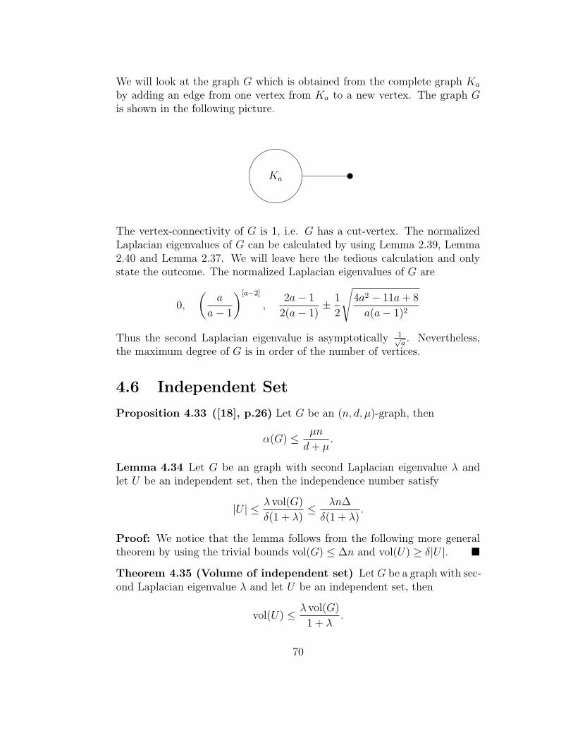
We will look at the graph G which is obtained from the complete graph Ka

by adding an edge from one vertex from Ka to a new vertex. The graph Gis shown in the following picture.

Ka

The vertex-connectivity of G is 1, i.e. G has a cut-vertex. The normalizedLaplacian eigenvalues of G can be calculated by using Lemma 2.39, Lemma2.40 and Lemma 2.37. We will leave here the tedious calculation and onlystate the outcome. The normalized Laplacian eigenvalues of G are

0,

(a

a − 1

)[a−2]

,2a − 1

2(a − 1)± 1

2

√

4a2 − 11a + 8

a(a − 1)2

Thus the second Laplacian eigenvalue is asymptotically 1√a. Nevertheless,

the maximum degree of G is in order of the number of vertices.

4.6 Independent Set

Proposition 4.33 ([18], p.26) Let G be an (n, d, µ)-graph, then

α(G) ≤ µn

d + µ.

Lemma 4.34 Let G be an graph with second Laplacian eigenvalue λ andlet U be an independent set, then the independence number satisfy

|U | ≤ λ vol(G)

δ(1 + λ)≤ λn∆

δ(1 + λ).

Proof: We notice that the lemma follows from the following more generaltheorem by using the trivial bounds vol(G) ≤ ∆n and vol(U) ≥ δ|U |.

Theorem 4.35 (Volume of independent set) Let G be a graph with sec-ond Laplacian eigenvalue λ and let U be an independent set, then

vol(U) ≤ λ vol(G)

1 + λ.

70

Proof: Because U is an independent set in G, it holds that e(U,U) = 0 andby Theorem 4.16 we have that

vol(U)2

vol(G)≤ λ

vol(U) vol(U)

vol(G)= λ

vol(U)(vol(G) − vol(U))

vol(G).

This implies that vol(U) ≤ λ vol(G)1+λ

.

Example 4.36 We look at the star Sn with n vertices. The second Laplacianeigenvalue of Sn is 1 (because Sn is bipartite; use Lemma 2.49). We havealso ∆ = n − 1 and δ = 1. So Lemma 4.34 would give us that the size ofany independent set in Sn is at most n − 1 which is a sharp bound. We canconclude with Theorem 4.35 that the volume of an independent set in Sn isat most n − 1. This bound is also sharp for Sn.

Question: How small can the second Laplacian eigenvalue be for graphs onn vertices with an independent set of size k?

We have seen in Example 4.18 a graph G on n = a + k vertices with anindependent set of size k and with second Laplacian eigenvalue

λ(G) =a + 2k − 1

a + k − 1− 1 =

k

a + k − 1= O(

k

n).

We will claim now that this is best possible. We state the following claim:

Claim: Let G be a connected graph on n vertices with normalized Laplacianeigenvalues λ1, . . . , λn with second Laplacian eigenvalue λ and independencenumber α. Then

λ ≥ α

n

Even

λn ≥ 1 +α

n=

n + α

n.

NOTE: We have no proof for the above claim. For d-regular graphs it fol-lows from Proposition 4.33. For some special cases we can apply Lemma 4.28to derive the claim but for general this seems not to work.

Nevertheless, we have written some procedures in the mathematical softwareMaple 9.0 (see Appendix) and so we checked the claim up to all graphs onat most 6 vertices. We have also calculate some randomly chosen graphs onmore than 6 vertices and the claim remains also for these graphs true. Thus,we have the impression that this claim should be true.

71

4.7 Colorability

Proposition 4.37 ([18], p.28) Let G be an (n, d, λ)-graph. Then the chro-matic number satisfies

χ(G) ≥ 1 + d/λ.

Lemma 4.38 Let G be a graph on n vertices with second Laplacian eigen-value λ. Then the chromatic number satisfies

χ(G) ≥ nδ(1 + λ)

λ vol(G)≥ δ(1 + λ)

λ∆

Proof: Every color class in the proper coloring of G forms an independentset. By using Lemma 4.34 we obtain:

χ(G) ≥ n

α(G)≥ nδ(1 + λ)

λ vol(G)≥ δ(1 + λ)

λ∆.

Question: What are the possible values for the second Laplacian eigenvalueof graphs on n vertices which are k-colorable? - We answer this question inthe following lemma.

Lemma 4.39 i) The minimum value for the second Laplacian eigenvalueover all graphs on n vertices which are k-colorable is 1

k−1(for at least infi-

nitely many n’s).

ii) The maximum value for the second Laplacian eigenvalue over all graphson n vertices which are k-colorable is 1.

Proof: i) Lemma 2.50 give us that every k-colorable graph has an eigenvaluewhich is at least k

k−1So the second Laplacian eigenvalue of a k-colorable graph

is at least 1k−1

. We look at Kk(s), i.e. the s-blow-up of the complete graphKk. Then Lemma 2.45 give us that the second Laplacian eigenvalue of Kk(s)is 1

k−1. So this proves the first the equality.

ii) We distinguish two cases. First assume that k = 1. Then the only1-colorable graphs are union of points and they have second Laplacian eigen-value 1. For k ≥ 2 we can take a bipartite graph which is then k-colorableand has second Laplacian eigenvalue 1.

72

4.8 Hamiltonicity

We will use the following theorem by Chvatal and Erdos

Proposition 4.40 ([28]) Let G be a graph with at least three vertices. If,for some s, G is s-connected and contains no independent set of size morethan s, then G is Hamiltonian.

Now, we can get a condition for the Hamiltonicity of a graph by combiningthis proposition with the Theorems 4.30 and 4.33.

Proposition 4.41 ([18], p.37) Let G be an (n, d, λ)-graph. If

d − 36λ2

d≥ λn

d + λ,

then G is Hamiltonian.

In the same way, by combining Proposition 4.40 with Theorem 4.31 and 4.34we get the following result.

Theorem 4.42 (Hamiltonicity) Let G be a graph on n vertices with sec-ond Laplacian eigenvalue λ. If

δ − 36λ2∆ ≥ nδ(1 + λ)

λ vol(G)

then G is Hamiltonian.

4.9 Small subgraphs

Proposition 4.43 ([24]) Let G be an (n, d, λ)-graph with at most one loopat each vertex. For every integer r ≥ 2 denote

sr =(λ + 1)n

d

(

1 +n

d+ ... +

(n

d

)r−2)

.

Then every set of more than sr vertices of G contains a copy of Kr.

We are not really interested in loops. So we will generalize this theorem forgraphs without loops. But a generalization with loops is also possible.

73

Theorem 4.44 (copy of Kr) Let G be a graph on n vertices with secondLaplacian eigenvalue λ. For every integer r ≥ 2 denote

sr = λ∆

(

∆n

δ2+

(∆n

δ2

)2

+ ... +

(∆n

δ2

)r−1)

.

Then every set of more than sr vertices of G contains a copy of the completegraph Kr

Proof: (induction over r):r=2: Let S ⊆ V (G) with |S| > s2 = λ∆2n

δ2 . With Theorem 4.15 we get

e(S, S) ≥ vol2(S)

vol(G)− λ vol(S) ≥ δ2|S|2

∆n− λ∆|S| >

δ2|S|∆n

· λ∆2n

δ2− λ∆|S| = 0.

So there is at least one edge in S, i.e. that the base case is proven.

r → r+1: Let S ⊆ V (G) with |S| > sr+1.

∑

v∈S

|NS(v)| = e(S, S) ≥ vol2(S)

vol(G)− λ vol(S) ≥ δ2|S|2

∆n− λ∆|S|.

It follows that there is a vertex v ∈ S such that

|NS(v)| ≥ δ2|S|∆n

− λ∆ >δ2sr+1

∆n− λ∆ = sr.

Using the induction hypothesis, we get that NS(v) contains a copy of Kr.Thus S contains a copy of Kr+1.

Proposition 4.45 ([18], p.32f) Let k ≥ 1 be an integer and let G be an(n, d, λ)-graph such that d2k/n λ2k−1. Then G contains a cycle of length2k + 1.

Theorem 4.46 (copy of cycle C2k+1) Let k ≥ 1 be an integer and let Gbe a graph with second Laplacian eigenvalue λ. If

λ2k−1 δ4k−2

n∆4k−3and λ = o

(δ4

∆4

)

(5)

then G contains a cycle of length 2k + 1.

74

Proof: Assumption: Suppose that G contains no cycle of length 2k + 1.For every two vertices u, v of G denote by d(u, v) the length of a shortestpath from u to v. For every i ≥ 1 let Ni(v) := u; d(u, v) = i be the set ofall vertices in G which are at distance exactly i from v. In [25] Erdos et al.proved that if G contains no cycle of length 2k+1 then for any 1 ≤ i ≤ k theinduces graph G[Ni(v)] contains an independent set of size|Ni(v)|/(2k − 1).Let v be a vertex with minimal degree, i.e. dv = δ. The above result togetherwith Theorem 4.34 implies that for every 1 ≤ i ≤ k the following holds

|Ni(v)| ≤ (2k − 1)∆λn

δ. (6)

Therefore by Theorem 4.15

e(Ni(v), Ni(v)) ≤ vol2(Ni(v))

vol(G)+ λ vol(Ni(v)) ≤ ∆2|Ni(v)|2

δn+ λ∆|Ni(v)|

(6)

≤ ∆2(2k − 1)∆λn|Ni(v)|δ2n

+∆2

δ2· λ∆|Ni(v)|

=2kλ|Ni(v)|∆3

δ2

(5)= o(

δ2

∆|Ni(v)|). (7)

Claim: For every 1 ≤ i ≤ k − 1 the following is true

|Ni+1(v)||Ni(v)| ≥ (1 − o(1))

δ4

∆4λ2.

We prove this claim by induction. By the above discussion the number ofedges spanned by N1(v) is o(δ2) and therefore

e(N1(v), N2(v)) = vol(N1(v)) − e(N1(v), N1(v)) − e(N1(v), v)(dv=δ)

≥ δ2 − o(δ2) = (1 − o(1))δ2.

On the other hand, by Theorem 4.15

e(N1(v), N2(v)) ≤ ∆2|N1(v)||N2(v)|δn

+ λ∆√

|N1(v)||N2(v)|

(7)

≤ ∆2

δn· ∆ · (2k − 1)∆λn

δ+ λ∆|N1(v)|

√

|N2(v)||N1(v)|

≤ O(λ∆4

δ2) + λ∆2

√

|N2(v)||N1(v)|

= o(δ2) + λ∆2

√

|N2(v)||N1(v)| .

75

Thus the base case is proven:

|N2(v)||N1(v)| ≥ (1 − o(1))

δ4

∆4λ2.

Now assume that |Ni(v)||Ni−1(v)| ≥ (1 − o(1)) δ4

∆4λ2 . We obtain

e(Ni(v), Ni+1(v)) = vol(Ni(v)) − e(Ni(v), Ni(v)) − e(Ni−1(v), Ni(v))(7)

≥ δ|Ni(v)| − o(δ2

∆|Ni(v)|) − ∆|Ni−1(v)|

(ind.)

≥ (1 − o(1))δ2

∆|Ni(v)| − ∆(1 + o(1))

∆4λ2

δ4|Ni(v)|

(5)= (1 − o(1))

δ2

∆|Ni(v)| − o(

δ4

∆3|Ni(v)|)

≥ (1 − o(1))δ2

∆|Ni(v)|.

On the other hand, by Theorem 4.15

e(Ni(v), Ni+1(v)) ≤ ∆2|Ni(v)||Ni+1(v)|δn

+ λ∆√

|Ni(v)||Ni+1(v)|

(6)

≤ ∆3(2k − 1)λ|Ni(v)|δ2

+ λ∆|Ni(v)|√

|Ni+1(v)||Ni(v)|

= o(δ2

∆|Ni(v)|) + λ∆|Ni(v)|

√

|Ni+1(v)||Ni(v)| .

Therefore |Ni+1(v)||Ni(v)| ≥ (1 − o(1)) δ4

∆4λ2 and we proved the induction step.

Finally note that

|Nk(v)| = δ

k−1∏

i=1

|Ni+1(v)||Ni(v)| ≥ (1 − o(1))δ

(δ4

∆4λ2

)k−1

= (1 − o(1))δ4k−3

λ2k−2∆4k−4

(5) (2k − 1)

∆λn

δ.

This is a contradiction (6).

76

Proposition 4.47 ([18], p.30) Let H be a fixed graph with r edges, svertices and maximum degree ∆, and let G = (V,E) be an (n, d, λ)-graph,

where, say, d ≤ 0.9n. Let m < n satisfy m λ(

nd

)∆. Then, for every subset

V ′ ⊂ V of cardinality m, the number of (not necessarily induced) copies ofH in V ′ is

(1 + o(1))ms

|Aut(H)|

(d

n

)r

.

Remark 4.48 i) Let us denote by copy(H,V ′) the number of not necessar-ily induced unlabeled copies of H in V ′. Let Aut(H) be the automorphismgroup of H. The number of not necessarily induced labeled copies of H inV ′ is equal to copy(H,V ′) · |Aut(H)|.

ii) We will use the notation of probability theory in the following. So wewrite the probability by P and the expectation by E.

Definiton 4.49 (conditional probability)

P[A|B] =P[A,B]

P[B]=

P[A and B]

P[B].

Lemma 4.50 Let X be a random variable and φ a measurable function andA,B some suitable sets. Then∑

k∈B

P[X ∈ A|φ(X) = k] · P[φ(X) = k|φ(X) ∈ B] = P[X ∈ A|φ(X) ∈ B].

Proof: We calculate∑

k∈B

P[X ∈ A|φ(X) = k]P[φ(X) = k|φ(X) ∈ B]

=∑

k∈B

P[X ∈ A, φ(X) = k]P[φ(X) = k, φ(X) ∈ B]

P[φ(X) = k]P[φ(X) ∈ B]

=∑

k∈B

P[X ∈ A, φ(X) = k]P[φ(X) = k

P[φ(X) = k]P[φ(X) ∈ B]

=∑

k∈B

P[X ∈ A, φ(X) = k]

P[φ(X) ∈ B]

=P[X ∈ A, φ(X) ∈ B]

P[φ(X) ∈ B]

= P[X ∈ A|φ(X) ∈ B].

77

Theorem 4.51 (number of copies) Let H be a fixed graph with r edgesand s vertices and maximum degree ∆(H). Let G = (V,E) be a graphon n vertices, maximum degree ∆ ≤ 0.9n, minimum degree δ and secondLaplacian eigenvalue λ. Let m < n satisfy

m λ∆

(∆3

δ3

)r (δn

∆2

)∆(H)

. (8)

Then, for every subset V ′ ⊆ V of cardinality m, the following holds

(1 + o(1))ms

|Aut(H)|

(δ2

∆n

)r

≤ copy(H,V ′) ≤ (1 + o(1))ms

|Aut(H)|

(∆2

δn

)r

.

Proof: We consider a random one-to-one mapping of the set of vertices ofH into the set of vertices V ′, i.e. all one-to-one mappings from V (H) to V ′

have the same probability.

Denote by A(H) the event that every edge of H is mapped on a edge of G.In such a case we say that the mapping is an embedding of H. It holds that

P[A(H)] =copy(H,V ′)

ms|Aut(H)| .

Thus it is enough to show the following claim

Claim:

(1 + o(1))

(δ2

∆n

)r

≤ P[A(H)] ≤ (1 + o(1))

(∆2

δn

)r

Proof of the claim: (induction over r)

r=0: If H has no edges then clearly P[A(H)] = 1, i.e. the claim is true.

r > 0: Suppose that the claim holds for all graphs with less than r edges,and let u, v be two vertices of H such that u ∼ v. Let Huv be the graphobtained from H by removing the edge u, v (and keeping all vertices). LetHu and Hv be the induced subgraphs of H on the sets of vertices V (H)\uand V (H) \ v, respectively. Let H ′ be the induced subgraph of H on theset of vertices V (H) \ u, v. Let r′ be the number of edges of H ′. Sinceu ∼ v we have

r − r′ ≤ 2(∆(H) − 1) + 1 = 2∆(H) − 1. (9)

78

By the definition of the conditional probability we get

P[A(H)] = P[A(H)|A(H ′)]P[A(H ′)]. (10)

Using Lemma 4.50

P[A(H)|A(H ′)] =∑

f ′∈A(H′)

P[A(H)| rest(f) = f ′] · P [rest(f) = f ′|A(H ′)]

= Ef ′ [P [A(H)| rest(f) = f ′]] (11)

where rest(f) denotes the restriction of the function f to the vertex set V (H ′)and Ef ′ [·] takes the expectation according to the induced probability distri-bution on rest(f).

For a fixed embedding f ′ from H ′, let Uf ′ be the vertex set of all possibleextension from f ′ to an embedding of Hu in V ′ and let Wf ′ be the vertexset of all possible extension from f ′ to an embedding of Hv in V ′. Denoteν(u, f ′) = |Uf ′ | and ν(v, f ′) = |Wf ′ |. Since u ∼ v we have e(Uf ′ ,Wf ′)many possibilities to extend f ′ to an embedding of H. Totally there arem1 · m2 := (m − s + 2)(m − s + 1) many possibilities to extend f ′. So

P[A(H)| rest(f) = f ′] =e(Uf ′ ,Wf ′)

(m − s + 2)(m − s + 1)=

e(Uf ′ ,Wf ′)

m1m2

.

By Lemma 4.15 we get

δ2

∆n

ν(u, f ′)ν(v, f ′)

m1m2

− ε ≤ P[A(H)| rest(f) = f ′] ≤ ∆2

δn

ν(u, f ′)ν(v, f ′)

m1m2

+ ε

(12)

where |ε| = λ∆

√ν(u,f ′)ν(v,f ′)

m1m2. We will see later that this “error term” will be

negligible.

How many extensions on an embedding f ′ of H ′ to an embedding of Huv

does exists? W.l.o.g. we can assume that ν(u, f ′) ≤ ν(v, f ′). By extendingstepwise, first to V (H ′) ∪ u and then to V (H) = V (H ′) ∪ u, v we get atleast ν(u, f ′)(ν(v, f ′)− 1) extensions and at most ν(u, f ′)ν(v, f ′) extensions.Thus

ν(u, f ′)ν(v, f ′) − ν(u, f ′)

m1m2

≤ P[A(Huv)| rest(f) = f ′] ≤ ν(u, f ′)ν(v, f ′)

m1m2

.

(13)

We show now that the expectation of the term − ν(u,f ′)m1m2

is negligible. By usingν(u, f ′) ≤ m we get

Ef ′ [ν(u, f ′)

m1m2

] ≤ m

m1m2

Ef ′ [1] = O(1

m).

79

If we show now that m → ∞ then indeed the above term is negligible. Byusing Lemma 4.17 we get λ = Ω( 1√

∆). Thus

m λ∆

(∆3

δ3

)r (δn

∆2

)∆(H)

= λ∆3r+1−2∆(H)n∆(H)

δ3r−∆(H)

≥ ∆3r−∆(H)

δ3r−∆(H)·√

∆n∆(H)

∆∆(H)≥ n∆(H)

∆∆(H)−1/2≥ n1/2

i.e. m → ∞ as n → ∞.

By taking the expectation Ef ′ over (13) and including that some term isnegligible, we become

Ef ′ [ν(u, f ′)ν(v, f ′)

m1m2

] =∑

f ′∈A(H′)

P[A(Huv)| rest(f) = f ′] · P[rest(f) = f ′|A(H ′)]

(Lem. 4.50)= P[A(Huv)|A(H ′)]

=P[A(Huv), A(H ′)]

P[A(H ′)]=

P[A(Huv)]

P[A(H ′)]. (14)

Altogether

P[A(H)](10),(11)

= Ef ′ [P[A(H)| rest(f) = f ′]] · P[A(H ′)](12)

≤ ∆2

δnEf ′ [

ν(u, f ′)ν(v, f ′)

m1m2

]P[A(H ′)] + α

(14)=

∆2

δn

P[A(Huv)]

P[A(H ′)]P[A(H ′)] + α

(ind.)

≤ (1 + o(1))

(∆2

δn

)r

+ α. (15)

where α = Ef ′ [|ε|] · P [A(H ′)]. In the same manner we get

P[A(H)] ≥ (1 + o(1))

(δ2

∆n

)r

− α.

Now, the only thing we have to check, is that the term α is negligible in

respect to the main term. Since(

δ2

∆n

)r

≤(

∆2

δn

)r

it is enough to show

α (

δ2

∆n

)r

.

80

We begin by using Jensen’s Inequality

α = Ef ′ [|ε|]P[A(H ′)]

≤ λ∆

√

Ef ′ [ν(u, f ′)ν(v, f ′)]

m1m2

P[A(H ′)]

(13)

≤ λ∆√m1m2

√

P[A(Huv)]

P[A(H ′)]P[A(H ′)]

(ind.)

≤ λ∆√m1m2

(1 + o(1))

(∆2

δn

)(r−1+r′)/2

Now, we have α (

δ2

∆n

)r

if

m λ∆

(∆2

δn

)(r−1+r′)/2(∆n

δ2

)r

(9)

≥ λ∆

(∆3

δ3

)r (δn

∆2

)∆(H)

which is exactly our assumption (8) on m.

81

Chapter 5

Turan’s Theorem

5.1 Classical Turan’s Theorem

Theorem 5.1 (Turan) ([15], p.42) If a graph G on n vertices has no(t + 1)-clique, t ≥ 2, then

|E(G)| ≤(

1 − 1

t

)n2

2.

Proof: (Induction over n)n=1: There is only one graph with one vertex and this graph has no t-cliquefor t ≥ 2 and has no edges.

n>1: Suppose now the inequality is true for all graphs on at most n − 1vertices, and let G be a graph on n vertices without (t + 1)-cliques and witha maximal number of edges. This graph certainly contains t-cliques, sinceotherwise we could add edges. Let A be a t-clique, and set B = V − A.

G[A] is the complete graph, so A contains e(A,A) = t(t − 1) edges. Byinduction, we have

e(B,B) ≤(

1 − 1

t

)

(n − t)2.

Since G has no (t+1)-clique, every x ∈ B is adjacent to at most t−1 verticesin A, and we obtain

e(A,B) ≤ (t − 1)(n − t).

83

Summing up

|E(G)| =e(A,A)

2+

e(B,B)

2+ e(A,B)

≤ t(t − 1)

2+

(

1 − 1

t

)(n − t)2

2+ (t − 1)(n − t)

=

(

1 − 1

t

)n2

2.

Definiton 5.2 (H-free, ex(G, H)) Let G,H be graphs. If G contains nocopy of H then we say that G is H-free. The Turan number ex(G,H) of Hin G is the largest integer e such that there is an H-free subgraph of G withe edges.

There are different viewpoints of Turan’s Theorem. First, the question arises,how do we construct an Kt+1-free graph with maximal number of edges?Well, we can look at the t-partite graphs which are Kt+1-free. The completet-partite graph on n vertices whose partite sets differs in size at most 1 iscalled Turan’s graph denoted by T (n, r). The size of each part is floor or ceilof n/r. Thus, it has

|E(T (n, t))| =

(

1 − 1

t

)n2

2

edges. (For n = αt this is exactly true and otherwise we have to take thefloor or ceil some numbers.) Turan’s Theorem says that this construction isbest possible.

Theorem 5.3 Among n vertex Kt+1-free graphs Turan graph T (n, r) hasthe most number of edges.

We can also start with the complete graph on n vertices. Then we will askhow many edges do we have to delete such that the remaining graph will beKt+1-free? Turan’s Theorem answer this question: We have to delete at least1t

n2

2edges. We note that the complete graph has n(n−1)

2edges. The difference

between n2

2and n(n−1)

2is very small. So we can also say by neglecting some

error term, that we have to delete at least 1t

of all edges in Kn to obtain anKt+1-free graph. We will state this in an asymptotic way:

Corollary 5.4 The maximum number of edges in an n-vertex Kt+1-freegraph is

ex(Kn, Kt+1) =

(t − 1

t+ o(1)

)n(n − 1)

2.

as n → ∞.

We will now look at generalizations of this result.

84

5.2 Generalization to (n, d, λ)-graphs

We will discuss here the paper of Sudakov, Szabo and Vu [2]. They generalizeTuran’s Theorem for (n, d, λ)-graphs.

Theorem 5.5 (Turan’s Theorem for (n, d, λ)-graphs) ([2]) Let t ≥ 3be an integer and let G be an (n, d, λ)-graph. If

dt−1

nt−2 λ

then

ex(G,Kt) =

(t − 2

t − 1+ o(1)

)

|E(G)|.

Let us check that Theorem 5.5 is indeed a generalization of Corollary 5.4.For that we observe that Kn is a (n−1)-regular graph with second adjacencyeigenvalue equal to 1 (cf. Example 4.18).

Now, we will outline the proof of Theorem 5.5. The idea is to prove the The-orem by induction over t and using the properties of pseudo-random graphssuch as Theorem 4.8 and Corollary 4.7 and also the Cauchy-Schwarz Inequal-ity. The problem with the induction is that a subgraph of a (n, d, λ)-graphhas not to be d-regular any more. For that, they introduce the technicalconcept of graphs which have the (t, p, δ)-property. For these graphs the in-duction works and the (n, d, λ)-graphs have the (t, p, δ)-property as shown in[2].

Definiton 5.6 ((t, p, δ)-property) Let G = (V,E) be a graph on n ver-tices, let t ≥ 2 be an integer and let δ(n) and p(n) be two functions of n suchthat 0 < p = p(n) ≤ 1 and δ(n) tends to zero when n tends to infinity. Wesay that G has the (t, p, δ)-property if it satisfies the following two conditions.

(i) For every two subsets U and W of V (G) of cardinality at least (δp)t−2n∣∣∣e(U,W ) − p|U ||W |

∣∣∣ ≤ δp|U ||W |

(ii) For every subset U of V (G) with cardinality at least (δp)t−3n there areat most (δp)t−1n vertices of G with

∣∣∣|NU(v)| − p|U |

∣∣∣ > δp|U |,

where NU(v) is the set of all neighbors of v in U .

85

5.3 Comments about Chung’s paper

There is an more general paper ([7]) by Chung for a spectral Turan theoremfor general graphs. This paper should appear soon. She uses the normalizedLaplacian instead of the adjacency. We have the impression that somethingis wrong in her paper. We begin with her main theorem.

Theorem 5.7 Let G be a graph on n vertices and second Laplacian eigen-value λ. If

λ = o

(1

vol−2t+3(G) vol(G)t−2

)

(1)

then any subgraph of G containing no Kt+1 has at most(

t − 1

t+ o(1)

)

|E(G)|

edges.

Definiton 5.8 (k-volume) Let U be a subset of the vertices and k a (pos-sibly negative) integer. Then we define the k-volume of U as

volk(U) =∑

u∈U

dku.

There is also used an inductive argument to prove Theorem 5.7. But for thatone has to state the above theorem in a more general way. Let R be any subsetof edges such that every Kt+1 in G contains at least one edge in R. In orderto prove Theorem 5.7, it is enough to show that |R| ≥ (1 + o(1))|E(G)|/t.Look at the following theorem

Theorem 5.9 Suppose a graph G on n vertices has second Laplacian eigen-value λ which satisfies (1). Let X be a subset of vertices in G and 0 < k ≤ tnonnegative integers. If R contains an edge from every complete subgraphon k + 1 vertices, then we have, for all i such that 0 ≤ i ≤ k,

∑

u∈X

∑

v∈X:u,v∈R

1

divd

iu

≥ vol2−i+1(X)

k vol(G)+ O

(

λk−1∑

j=0

vol−2i−2j+1(X) volj(G)

)

.

Remark 5.10 First, let us chose i = 0 and X = V (G) in the above lemma.Then we get

2|R| ≥ vol2(G)

k vol(G)+ ε =

1

k2|E(G)| + ε

where ε is the error term. By some calculation about the error term one canconclude Theorem 5.7 from Theorem 5.9.

86

To prove Theorem 5.9 Chung needs a lot of lemmas. The first three lemmasdescribe the edge distribution of pseudo-random graphs; they look all fine.The next lemmas look not so fine. We will here state these lemmas and showwhy we think that they are wrong. Also we will extract some claims aboutthe negligence of some λ2-terms and look at them.

5.3.1 Lemmas

Lemma 5.11 (Lemma 4 in Chung’s paper [7]) Suppose a graph G on nvertices has second Laplacian eigenvalue less than δ. Suppose X is a subsetof vertices of G. For v a vertex in X, let ΓX(v) denote the neighborhood ofv in X and let R(v) denote a subset of Γ(v). We have

∑

v∈X

|ΓX(v)|2dv

≥ vol3(X)

vol2(G)+ O(δ

vol2(X)

vol(G)) + O(δ2 vol(X)). (2)

and∑

v∈X

|ΓX(v)||R(v)|dv

≤∑

v∈X

|R(v)| vol(X)

vol(G)+ δ

vol2(X)

vol(G). (3)

In this Lemma the second inequality seems to be wrong. Consider the fol-lowing counterexample.

Example 5.12 Let G = Cn be a cycle with n vertices and let δ = 1,say. Since G is 2-regular we have for every subset U of the vertices thatvol(U) = 2|U |.

Let X be any subset of vertices such that for all v ∈ X it holds |ΓX(v)| ≥ 1and let R(v) = uv be a single vertex with v ∼ uv for all v ∈ X. So wehave that every vertex v has at least one neighbor in X and the set R(v)contains exactly one element. Thus, the left hand side (LHS) and right handside (RHS) of (3) are

LHS =∑

v∈X

|ΓX(v)||R(v)|dv

≥∑

v∈X

1

2=

|X|2

.

RHS =∑

v∈X

|R(v)| vol(X)

vol(G)+ δ

vol2(X)

vol(G)

= |X|vol(X)

vol(G)+ δ

vol2(X)

vol(G)

=|X|2n

+2|X|2

n.

87

If |X| = o(n), then the LHS ≥ RHS, contradicting Lemma 5.11.

Lemma 5.13 (Lemma 5 in Chung’s paper [7]) Suppose a graph on nvertices has second Laplacian eigenvalue less than δ. Suppose X is a subsetof vertices of G and i is a nonnegative value. We have

∑

v∈X

1

di+1v

(vol−i(ΓX(v)))2 =vol3−i+1(X)

vol2(G)+ O(δ

vol−i+1(X) vol−2i+1(X)

vol(G)) (4)

and

∑

v∈X

1

di+1v

vol−i(ΓX(v)) vol−i(R(v)) =

=vol−i+1(X)

vol(G)

∑

v∈X

∑

u∈R(v)

1

divd

iu

+ O(δvol−i+1(X) vol−2i+1(X)

vol(G). (5)

The second equation seems to be wrong. We use the same example as above.This gives us:

LHS =∑

v∈X

1

di+1v

vol−i(ΓX(v)) vol−i(R(v))

≥ |X| 1

2i+12−i2−i

= 2−3i−1|X|.

RHS =vol−i+1(X)

vol(G)

∑

v∈X

∑

u∈R(v)

1

divd

iu

+ O

(

δvol−i+1(X) vol−2i+1(X)

vol(G)

)

=|X|2−i+1

2n|X| 1

2i2i+ O

( |X|2−i+1 · |X|2−2i+1

2n

)

= 2−3i |X|2n

+ O

(

2−3i+1 |X|2n

)

.

Again, for some X, with |X| = o(n), the RHS is of smaller order than theLHS, which would contradict the second equation of Lemma 5.13.

Lemma 5.14 (Lemma 6 in Chung’s paper [7]) Suppose that X is asubset of vertices in a graph G and α ≤ β are positive values. Then

vol−α(X) vol−β(X) ≤ vol−α+1(X) vol−β−1(X).

88

Remark 5.15 This lemma should be stated at least for the case 0 ≤ α ≤ β,i.e. α can be zero. Because when Chung needs the lemma on page 12, sheexactly needs the case that α = 0 and β = −2j. We have proved this lemmain a more general case in Chapter 3 (see Lemma 3.2).

5.3.2 Negligence of the λ2-term

We will now analyze some points in the process of the proof of Theorem 5.9from the paper [7]. For that we assume that we have a graph G on n verticesand second Laplacian eigenvalue λ such that (1) holds.

On page 11 in the second paragraph there is mentioned, that the termsinvolving λ2 are of lower order than the terms involving λ by using theassumption (1) on λ. So Chung claims the following:

λ2

k−2∑

j=0

√

vol−1(X) vol−4j−1(X) volj(G) = o

(

λk−2∑

j=0

|X| vol−2j(X) volj(G)

vol(G)

)

This claim seems to be wrong. Consider the following example:

Example 5.16 Let G be the Payley-graph Pq which has n = q vertices andis d-regular with d = n−1

2≈ n

2. By Example 4.11 and Theorem 2.20 we

know that the second Laplacian eigenvalue λ of Pq fulfills λ ≈ 1√n. The

Payley-graph fulfills the assumption (1) because

1

vol−2t+3(G) vol(G)t−2=

1

d−2t+3n · dt−2nt−2=

dt−1

nt−1= O(1).

Then

LHS = λ2∑

√

|X|d

d−4j−1|X|(dn)j ≈ 1

n

∑

|X|njd−j−1 ≈ |X|2k

n2.

RHS = λ∑ |X|d−2j|X|(nd)j

nd≈ 1√

n

∑

|X|2nj−1d−j−1 ≈ |X|2 2k

n2.5

If |X| = o(n1/2), then the RHS is tending faster to 0 than the LHS. Thiscontradicts the above claim.

89

On page 11 at line 14 there is mentioned, that the terms involving λ2 can beignored by using the assumption on λ. So Chung claims the following:

λ2 vol(X) = o

(

λvol2(X)

vol(G)

)

.

Consider again the above example. We obtain

LHS = λ2|X|d ≈ |X|2

.

RHS = λ|X|2d2

nd≈ |X|2

2√

n.

This is a contradiction to the above claim if |X| = o(√

n).

90

Appendix

List of Definitions

2.1 adjacency matrix . . . . . . . . . . . . . . . . . . . . . . . . . . . 132.2 adjacency eigenvalues . . . . . . . . . . . . . . . . . . . . . . . . . 142.7 Laplacian . . . . . . . . . . . . . . . . . . . . . . . . . . . . . . . 162.10 Laplacian eigenvalues . . . . . . . . . . . . . . . . . . . . . . . . . 182.13 normalized Laplacian . . . . . . . . . . . . . . . . . . . . . . . . . 192.15 normalized Laplacian eigenvalues . . . . . . . . . . . . . . . . . . 202.22 nonnegative, positive matrices . . . . . . . . . . . . . . . . . . . . 232.23 incomposable/decomposable . . . . . . . . . . . . . . . . . . . . . 242.34 strongly regular graph . . . . . . . . . . . . . . . . . . . . . . . . 302.38 twins . . . . . . . . . . . . . . . . . . . . . . . . . . . . . . . . . . 322.44 k-blow-up . . . . . . . . . . . . . . . . . . . . . . . . . . . . . . . 352.54 interlace . . . . . . . . . . . . . . . . . . . . . . . . . . . . . . . . 392.64 decreasing rearrangement . . . . . . . . . . . . . . . . . . . . . . 442.65 majorize . . . . . . . . . . . . . . . . . . . . . . . . . . . . . . . . 443.7 spectral norm . . . . . . . . . . . . . . . . . . . . . . . . . . . . . 503.9 spectral radius . . . . . . . . . . . . . . . . . . . . . . . . . . . . 514.1 random graph . . . . . . . . . . . . . . . . . . . . . . . . . . . . . 554.2 e(U,W ) . . . . . . . . . . . . . . . . . . . . . . . . . . . . . . . . 564.4 random graph with given degree distribution . . . . . . . . . . . . 564.5 second adjacency eigenvalue . . . . . . . . . . . . . . . . . . . . . 574.6 (n, d, λ)-graph . . . . . . . . . . . . . . . . . . . . . . . . . . . . . 574.12 second Laplacian eigenvalue . . . . . . . . . . . . . . . . . . . . . 604.14 volume . . . . . . . . . . . . . . . . . . . . . . . . . . . . . . . . . 604.20 dU . . . . . . . . . . . . . . . . . . . . . . . . . . . . . . . . . . . 644.49 conditional probability . . . . . . . . . . . . . . . . . . . . . . . . 775.2 H-free, ex(G,H) . . . . . . . . . . . . . . . . . . . . . . . . . . . 845.6 (t, p, δ)-property . . . . . . . . . . . . . . . . . . . . . . . . . . . . 855.8 k-volume . . . . . . . . . . . . . . . . . . . . . . . . . . . . . . . . 86

91

List of Theorems

1.3 Whitney . . . . . . . . . . . . . . . . . . . . . . . . . . . . . . . . 91.4 Tutte’s 1-Factor Theorem . . . . . . . . . . . . . . . . . . . . . . 91.8 Spectral Theorem . . . . . . . . . . . . . . . . . . . . . . . . . . . 101.9 Rayleigh-Ritz . . . . . . . . . . . . . . . . . . . . . . . . . . . . . 111.11 Courant-Fischer . . . . . . . . . . . . . . . . . . . . . . . . . . . . 111.12 positive semidefinite matrices . . . . . . . . . . . . . . . . . . . . 112.20 Relations for d-regular graphs . . . . . . . . . . . . . . . . . . . . 222.25 Perron-Frobenius . . . . . . . . . . . . . . . . . . . . . . . . . . . 242.28 eigenvalues of bipartite graphs . . . . . . . . . . . . . . . . . . . . 262.30 Number of Walks . . . . . . . . . . . . . . . . . . . . . . . . . . . 272.52 Interlacing . . . . . . . . . . . . . . . . . . . . . . . . . . . . . . . 392.53 Interlacing for the adjacency matrix . . . . . . . . . . . . . . . . . 392.57 Interlacing for the Laplacian . . . . . . . . . . . . . . . . . . . . . 402.62 Gerschgorin . . . . . . . . . . . . . . . . . . . . . . . . . . . . . . 422.66 Schur’s Majorization Theorem . . . . . . . . . . . . . . . . . . . . 443.1 Cauchy-Schwarz inequality . . . . . . . . . . . . . . . . . . . . . . 473.4 Chebyshev-Inequality . . . . . . . . . . . . . . . . . . . . . . . . . 493.5 General Cauchy-Schwarz Inequality . . . . . . . . . . . . . . . . . 503.12 Cauchy-Schwarz reformulation . . . . . . . . . . . . . . . . . . . . 523.15 subtracting eigenvectors . . . . . . . . . . . . . . . . . . . . . . . 524.3 random graph: edge distribution . . . . . . . . . . . . . . . . . . 564.7 (n, d, λ)-graph: edge distribution . . . . . . . . . . . . . . . . . . 574.9 (n, d, λ)-graph: edge distribution . . . . . . . . . . . . . . . . . . 594.15 second Laplacian eigenvalue: edge-distribution . . . . . . . . . . . 614.16 second Laplacian eigenvalue: edge-distribution . . . . . . . . . . . 614.22 δ-edge-connected . . . . . . . . . . . . . . . . . . . . . . . . . . . 644.31 vertex connectivity . . . . . . . . . . . . . . . . . . . . . . . . . . 684.35 Volume of independent set . . . . . . . . . . . . . . . . . . . . . . 704.42 Hamiltonicity . . . . . . . . . . . . . . . . . . . . . . . . . . . . . 734.44 copy of Kr . . . . . . . . . . . . . . . . . . . . . . . . . . . . . . . 744.46 copy of cycle C2k+1 . . . . . . . . . . . . . . . . . . . . . . . . . . 744.51 number of copies . . . . . . . . . . . . . . . . . . . . . . . . . . . 785.1 Turan . . . . . . . . . . . . . . . . . . . . . . . . . . . . . . . . . 835.5 Turan’s Theorem for (n, d, λ)-graphs . . . . . . . . . . . . . . . . 85

92

Maple-Code

We will describe below some Maple-Code which we used to verify some state-ments on some exemplary graphs. We used the mathematical software Maple

9 by Maplesoft. The (standard) commands for graphs are in a package called“networks” and the commands for linear algebra are in a package called“linalg”. So first one should include these two packages:

with(networks):with(linalg):

The command adjacency(G) will compute the adjacency matrix of a graphG. There is no command for the Laplacian or the normalized Laplacian. Sowe have defined the normalized Laplacian matrix in the following procedure:

lap := proc(G)

local n,vert,k,seq_degree,M,a,b:

n := nops(vertices(G)):

vert := convert(vertices(G),list):

seq_degree := seq(vdegree(vert[k],G),k=1..n):

M:=Matrix(1..n,1..n);

for a from 1 to n do

for b from 1 to n do

if evalb( vert[a] in neighbors(vert[b],G) ) then

M[a,b] := -1/sqrt(seq_degree[a]*seq_degree[b]):

end if:

od:

M[a,a] := 1;

od:

return M:

end:

In the following we will describe a procedure for calculating the maximal sizeof an independent set of a graph G, i.e. for α(G). The idea is that we go overall subsets of the vertices and then check if they build an independent set.If this is so then we compare this size of the independent set with the bestpossible size by now and update this value. We note that the complexity issomething like 2n(G). So one should only try small graphs (with less than 10vertices or so).

indep := proc(G)

local n, alpha, A, z, test_vert, test_vect, l:

n := nops(vertices(G)):

93

alpha := 0:

A := adjacency(G):

for z from 1 to 2^n-1 do

test_vert := :

test_vect := vector(n,0):

for l from 1 to n do

if(z mod 2^l > 2^(l-1)-1) then

test_vert := test_vert union l: test_vect[l]:=1

end if:

od:

if evalb(multiply(test_vect,A,test_vect)=0

and nops(test_vert)>alpha) then

alpha := nops(test_vert):

end if:

od:

return alpha:

end proc

For verifying the statement

λ(G) ≥ α(G)

n

for all graphs on n vertices we can use the following procedure. We note thatthis procedure uses the the procedure lap(G) and indep(G). So this test isonly practical for small n.

poss_edg := :

for j from 1 to n do

for k from j+1 to n do

poss_edg := poss_edg union j,k:

od:

od:

poss_edg;

for z from 0 to 2^e-1 do

G := void(n):

for l from 1 to e do

if(z mod 2^l > 2^(l-1)-1) then addedge(poss_edg[l],G) end if:

od:

if(nops(components(G))=1) then

eig := evalf(Eigenvals(evalm(lap(G)))):

94

lambda := eig[n]-1:#max(1-eig[2], eig[n]-1):

alpha := indep(G):

if evalb(lambda<alpha/n) then

print(draw(G)):

end if:

end if:

od:

95

Bibliography

[1] I. Olkin A. W. Marshall. Inequalities: Theory of Majorization and itsApplications, volume 143 of Mathematics in Science and Engineering.Academic Press, 1979.

[2] T. Szabo B. Sudakov and V. H. Vu. A generalization of turan’s theorem.Journal of Graph Theory, to appear.

[3] N. Biggs. Algebraic Graph Theory. Cambridge University Press, 1974.

[4] G. Royle C. Godsil. Algebraic Graph Theory. Springer, 2001.

[5] D. K. Callebaut. Generalization of the cauchy-schwarz inequality. Jour-nal of mathematical analysis and applications, 12:491–494, 1965.

[6] F. Chung. Spectral Graph Theory. American Mathematical Society,National Science Foundation, 1997.

[7] F. Chung. A spectral turan theorem. Combinatorics, Probability andComputing, to appear. http://www.math.ucsd.edu/ fan/.

[8] S. S. Dragomir. personal communication.

[9] S. S. Dragomir. A survey on cauchy-bunyakovsky-schwarz type discreteinequalities. Journal of Inequalities in Pure and Applied Mathematics,4(3), 2003. http://jipam.vu.edu.au.

[10] L. Lu F. Chung. The average distance in a random graph with givenexpected degrees. Internet Mathematics, 1:91–114, 2003.

[11] F. R. Gantmacher. Matrizentheorie. Springer, 1986.

[12] F. Goldberg. Laplacians of graphs, quasi-strongly regular graphs andcompletely positive graphs. Master’s thesis, Technion - Israel Instituteof Technology, 2004. http://tx.technion.ac.il/ felixg/research.html.

97

[13] F. Harary. The determinant of the adjacency matrix. SIAM Review,4(3):202–210, 1962.

[14] F. Harary. Determinants, permanents and bipartite graphs. Mathemat-ics Magazine, 21:146–148, 1969.

[15] S. Jukna. Extremal Combinatorics. Springer, 2001.

[16] H. Sachs M. Cvetkovic, M. Doob. Spectra of Graphs. Johann AmbrosiusBarth, 3rd edition, 1995.

[17] D. J. Watts M. E. J. Newman, S. H. Strogatz. Random graphs witharbitrary degree distributions and their applications. Physical ReviewE, 64(2), 2001.

[18] B. Sudakov M. Krivelevich. Pseudo-random graphs. Preprint, submit-ted. http://www.math.tau.ac.il/ krivelev/prsurvey.ps.

[19] T. Szabo M. Krivelevich, B. Sudakov. Triangle factors in sparse pseudo-random graphs. Combinatorica, 24(3):403–426, 2004.

[20] H. W. McLaughlin and F. T. Metcalf. Remark on a recent generalizationof the cauchy-schwarz inequality. Journal of mathematical analysis andapplication, 18:522–523, 1967.

[21] D.S. Mitrinovic, J.E.Pecaric, and A.M. Fink. Classical and New Inequal-ities, volume 61 of Mathematics and its applications. Kluwer AcademicPublishers, 1993.

[22] B. Mohar. Some applications of laplace eigenvalues of graphs. in”Graph Symmetry: Algebraic Methods and Applications,” Eds. G.Hahn and G. Sabidussi, NATO ASI Ser. C 497, 497:225–275, 1997.http://www.fmf.uni-lj.si/ mohar/.

[23] J. Spencer N. Alon. The probabilistic method. Wiley, 2nd edition, 2000.

[24] M. Krivelevich N. Alon. Constructive bounds for a ramsey-type problem.Graphs and Combinatorics, 19:217–225, 1997.

[25] C. Rousseau P. Erdos, R. Faudree and R. Schelp. On cycle-completegraph ramsey numbers. Journal of Graph Theory, 2:53–64, 1978.

[26] C. R. Johnson R. A. Horn. Matrix Analysis. Cambridge UniversityPress, 1985.

98

[27] D. A. Spielman. Lectures in “spectral graph theory and its applications”(yale), 2004. http://www-math.mit.edu/ spielman/eigs/.

[28] P. Erdos V. Chvatal. A note on hamiltonian circuits. Discrete Mathe-matics, 2:111–113, 1972.

[29] E. R. van Dam. Graphs with few eigenvalues - An interplay be-tween combinatorics and algebra. PhD thesis, Tilburg University, 1996.http://center.uvt.nl/staff/dam/proefschrift.pdf.

[30] D. B. West. Introduction to Graph Theory. Prentice Hall, 2nd edition,2001.

99

comparison of spectral methods through the adjacency matrix and

Documents