comparison of shear-wave slowness proﬁles at 10 · pdf filecomparison of shear-wave slowness...

3116

Bulletin of the Seismological Society of America, Vol. 92, No. 8, pp. 3116–3133, December 2002

Comparison of Shear-Wave Slowness Profiles at 10 Strong-Motion Sites

from Noninvasive SASW Measurements and Measurements

Made in Boreholes

by Leo T. Brown,* David M. Boore, and Kenneth H. Stokoe II

Abstract The spectral-analysis-of-surface-waves (SASW) method is a relativelynew in situ method for determining shear-wave slownesses. All measurements aremade on the ground surface, making it much less costly than methods that requireboreholes. The SASW method uses a number of active sources (ranging from a com-mercial Vibroseis truck to a small handheld hammer for the study conducted here)and different receiver spacings to map a curve of apparent phase velocity versusfrequency. With the simplifying assumption that the phase velocities correspond tofundamental mode surface waves, forward modeling yields an estimate of the sub-surface shear-wave slownesses.

To establish the reliability of this indirect technique, we conducted a blind eval-uation of the SASW method. SASW testing was performed at 10 strong-motion sta-tions at which borehole seismic measurements were previously or subsequentlymade; if previously made, the borehole results were not used for the interpretationof the SASW data, and vice-versa.

Comparisons of the shear-wave slownesses from the SASW and borehole mea-surements are generally very good. The differences in predicted ground-motion am-plifications are less than about 15% for most frequencies. In addition, both methodsgave the same NEHRP site classification for seven of the sites. For the other threesites the average velocities from the downhole measurements were only 5–13 m/seclarger than the velocity defining the class C/D boundary. This study demonstratesthat in many situations the SASW method can provide subsurface information suitablefor site response predictions.

Introduction

In situ shear-wave slowness profiles are used in a varietyof earthquake engineering applications, including site re-sponse studies, liquefaction analyses, and soil–structure in-teraction evaluations. Borehole seismic methods such as thecrosshole and downhole methods traditionally have beenemployed to measure shear-wave slowness (slowness is sim-ply the reciprocal of velocity) in the field, since they aredirect measurements. More recently, a suspension logger(made by the Oyo Corporation) has been used for this pur-pose, particularly in boreholes with depths of 100 m andmore (the data from this instrument is referred to here as aPS log). Until now, seismic surface-wave methods, involv-ing either Love or Rayleigh waves, have received little at-tention. Surface-wave methods involve more assumptions,unknowns, and numerical simulations than borehole meth-

*Present address: Phillips Petroleum, 680-B Plaza Office Building, Bar-tlesville, Oklahoma 74004; e-mail: [email protected].

ods. Surface-wave methods, however, offer the advantage ofbeing noninvasive; hence, they are less costly and more rap-idly conducted than borehole methods. A number of studieshave inverted surface-wave phase velocities, obtained fromboth passive and active sources, to derive near-surface ma-terial properties (e.g., Horike, 1985; Zywicki, 1999); in thisstudy we use a particular method known as the spectral-analysis-of-surface-waves (SASW) method (Stokoe et al.,1994). The reliability of the SASW method needs to be es-tablished for it to gain widespread use in earthquake engi-neering.

Following the 1994 Northridge, California, earthquake,the U.S. Geological Survey drilled a number of boreholes atsites from which recordings of the ground motion were ob-tained (Gibbs et al., 1999). Several of the authors realizedthat this presented an excellent opportunity to test the SASWmethod at borehole sites. SASW measurements at a numberof these sites were made in the summer of 1997, and inter-

Comparison of Shear-Wave Slowness Profiles at 10 Strong-Motion Sites 3117

0 0.1 0.2 0.3 0.4 0.50

20

40

60

80

100

Poisson’s Ratio

Dep

th(m

)

from USGS OFR 99-446from USGS OFR 00-470from USGS OFR 01-506

Above water table

0 0.1 0.2 0.3 0.4 0.5

Poisson’s Ratio

from USGS OFR 99-446from USGS OFR 00-470from USGS OFR 01-506

Below water table

Figure 1. Poisson’s ratio versus depth for material above and below the water table,using values from recent measurements of velocities in southern California (Gibbs etal. 1999, 2000, 2001). The length of each vertical line spans the depth range for eachparticular constant-velocity layer from which Poisson’s ratio was determined. All ex-cept one of the few values in the righthand plot, for which Poisson’s ratio is less than0.4, correspond to cases for which the S velocity is high (i.e., rock, where the P velocityis not controlled by water velocity). The one exception is a “dry” layer below the watertable (with low P velocity).

pretation of the measurements was done in a truly blind man-ner, using no information from the downhole measurements.These results are contained in the Master’s thesis of the firstauthor (Brown, 1998). While preparing those results forpublication, it was discovered that Brown (1998) used thecommon assumption that Poisson’s ratio was 0.25 in hismodeling of the observed dispersion. Although a good as-sumption for most of the Earth, as shown in Figure 1, it isa poor assumption for near-surface soil that is saturated. Thisis so because the compressional wave velocity is controlledby the velocity of water (around 1500 m/sec) and is not wellcorrelated with shear-wave velocity, and as a result, Pois-son’s ratio can approach 0.5 in the saturated materials. Theassumption of 0.25 for Poisson’s ratio produces P-waveslownesses that are too high below the water table, and fit-ting the dispersion data then leads to S-wave slownesses thatin general are systematically low. Because of the anticipatedsystematic changes in the derived slownesses, we decided toreinterpret the data. To preserve the blind nature of the study,the files containing the dispersion curves were assigned non-sensical names by the second author (D.M.B.) and sent tothe first author (L.T.B.), who derived the slowness modelsfrom these randomly named files without use of previousresults or site information. The approximate water-tabledepth was given to L.T.B. by D.M.B., since this informationis generally available from a geologic investigation or could

be obtained from a P-wave refraction survey (the term“water table” is loosely used here to represent the top of thesaturated zone). In the modeling, Poisson’s ratio was as-sumed equal to 0.33 above the water table; below the watertable Poisson’s ratio was calculated using a compressionalvelocity equal to 1500 m/sec or with Poisson’s ratio equalto 0.25, if greater.

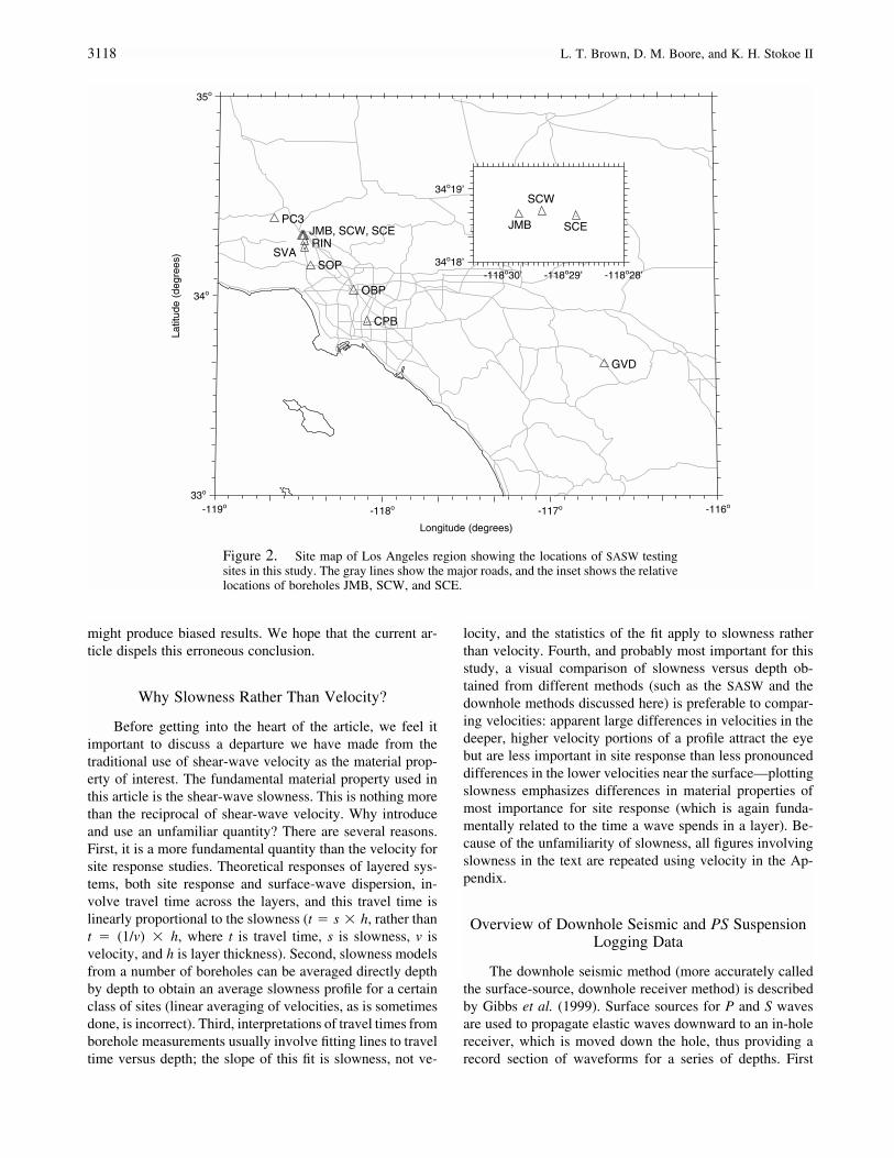
In this article we compare results from the SASWmethod and borehole measurements (both downhole logsand PS logs, if available) at 10 sites. These sites are shownin Figure 2, with additional information contained in Table1. We first give an overview of the borehole and the SASWmethods. This is followed by a presentation of results at twosites for which the comparisons were good and not so good(but for a known reason). Finally, we compare results for all10 sites. We find that overall the SASW results compare fa-vorably with the borehole results. The favorable comparisondiffers from that found in a previous article (Boore andBrown, 1998a,b). The earlier article compared shear-wavevelocities from borehole results and a specific application ofa by-now outdated noninvasive procedure, and the conclu-sions were intended to warn users that the results of thatapplication might contain biases. Our earlier article con-tained no conclusions regarding other noninvasive methods,although we fear that a number of readers misinterpreted ourresults to indicate that in general surface-wave methods

3118 L. T. Brown, D. M. Boore, and K. H. Stokoe II

-119o-118o -117o -116o

33o

34o

35o

Longitude (degrees)

Latit

ude

(deg

rees

)

CPB

GVD

JMB, SCW, SCERIN

SVASOP

OBP

PC3

-118o30’ -118o29’ -118o28’34o18’

34o19’

JMB

SCW

SCE

Figure 2. Site map of Los Angeles region showing the locations of SASW testingsites in this study. The gray lines show the major roads, and the inset shows the relativelocations of boreholes JMB, SCW, and SCE.

might produce biased results. We hope that the current ar-ticle dispels this erroneous conclusion.

Why Slowness Rather Than Velocity?

Before getting into the heart of the article, we feel itimportant to discuss a departure we have made from thetraditional use of shear-wave velocity as the material prop-erty of interest. The fundamental material property used inthis article is the shear-wave slowness. This is nothing morethan the reciprocal of shear-wave velocity. Why introduceand use an unfamiliar quantity? There are several reasons.First, it is a more fundamental quantity than the velocity forsite response studies. Theoretical responses of layered sys-tems, both site response and surface-wave dispersion, in-volve travel time across the layers, and this travel time islinearly proportional to the slowness (t � s � h, rather thant � (1/v) � h, where t is travel time, s is slowness, v isvelocity, and h is layer thickness). Second, slowness modelsfrom a number of boreholes can be averaged directly depthby depth to obtain an average slowness profile for a certainclass of sites (linear averaging of velocities, as is sometimesdone, is incorrect). Third, interpretations of travel times fromborehole measurements usually involve fitting lines to traveltime versus depth; the slope of this fit is slowness, not ve-

locity, and the statistics of the fit apply to slowness ratherthan velocity. Fourth, and probably most important for thisstudy, a visual comparison of slowness versus depth ob-tained from different methods (such as the SASW and thedownhole methods discussed here) is preferable to compar-ing velocities: apparent large differences in velocities in thedeeper, higher velocity portions of a profile attract the eyebut are less important in site response than less pronounceddifferences in the lower velocities near the surface—plottingslowness emphasizes differences in material properties ofmost importance for site response (which is again funda-mentally related to the time a wave spends in a layer). Be-cause of the unfamiliarity of slowness, all figures involvingslowness in the text are repeated using velocity in the Ap-pendix.

Overview of Downhole Seismic and PS SuspensionLogging Data

The downhole seismic method (more accurately calledthe surface-source, downhole receiver method) is describedby Gibbs et al. (1999). Surface sources for P and S wavesare used to propagate elastic waves downward to an in-holereceiver, which is moved down the hole, thus providing arecord section of waveforms for a series of depths. First


Table 1Borehole Information

Distance (m) V30 (m/sec) Class

Borehole Name Code Lat. (�) Long. (�) CL CD DH SASW DH SASW

Cerritos College: Police Building CPB 33.88212 �118.0968 76 2 250 234 D DGarner Valley Downhole Array GVD 33.6688 �116.673 5 5 282 275 D DJensen Filtr. Plant: Admin. Bldg JMB 34.3111 �118.4957 76 18 373 298 C DObregon Park OBP 34.03699 �118.17781 205 198 349 300 D DPotrero Canyon: Borehole 3 PC3 34.39522 �118.66317 4 4 205 246 D DRinaldi Receiving Station RIN 34.281 �118.4771 62 3 333 321 D DSylmar Converter Station East SCE 34.31077 �118.47986 72 6 370 323 C DSylmar Converter Station West SCW 34.3117 �118.4893 23 20 251 260 D DSherman Oaks Park SOP 34.1607 �118.4394 35 19 301 270 D DSepulveda V. A. Hospital SVA 34.249 �118.4772 52 50 365 285 C D

CL and CD are the distances from the borehole to the centerline and to the point of closest approach of the SASW linear array; Class is the NEHRP siteclass, defined by V30.

arrivals are fit using a least-squares procedure with a modelconsisting of constant velocity, laterally uniform layers. Therefraction of the rays between layers is taken into accountin the analysis. In a sense, the model represents materialproperties averaged laterally from the borehole over a dis-tance of a fraction of a wavelength (10 m is a typical wave-length for S waves in soils at the frequencies produced bythe S-wave source). Additionally, as with all wave-arrivalmethods, the stiffest materials in the borehole vicinity aremeasured.

The PS suspension logging method is described by Nig-bor and Imai (1994). A probe with a seismic source and tworeceivers is used to make interval P- and S-wave arrivals fora series of borehole depths, from which slowness or velocitycan be computed. High resolution data can be obtained(every 0.5 m) with no decrease in resolution with depth. Dataquality depends on borehole conditions. The best results areobtained for an uncased borehole. On the other hand, thedownhole logging method requires cased holes (in order toclamp the receiver at various depths), and therefore all holesdiscussed in this article were cased. Fortunately, casing ofthe holes drilled for the downhole logging was usually post-poned until the day after the drilling was completed. Thisallowed time for PS logging in the evening after the holeswere drilled, but before they were cased.

Overview of SASW Method

Spectral-analysis-of-surface-waves (SASW) testing, ini-tially developed at the University of Texas at Austin, is anin situ seismic method for determining shear-wave velocityor slowness profiles (Stokoe et al., 1989, 1994; Nazarian andStokoe, 1984). It is noninvasive and nondestructive, with alltesting performed on the ground surface at strain levels inthe soil in the elastic range (shear strains � 0.001%). Adetailed description of the SASW field procedure is given inBrown (1998) and Joh (1997). A vertical dynamic load isused as the source of the waves. For this investigation, aVibroseis truck, commonly used for seismic exploration in

the oil industry, was used to generate the long wavelengths.Various handheld hammers were used for the short wave-lengths. The ground motions were monitored by two verticalreceivers (70% critically damped 1-Hz geophones) and re-corded by a dynamic signal analyzer. A schematic of this isshown in Figure 3. To minimize phase shifts due to differ-ences in receiver coupling and subsurface variability, thesource location was reversed. Theoretical as well as practicalconsiderations, such as attenuation, necessitated the use ofseveral receiver spacings (generally keeping the same cen-terpoint for the array) to generate the dispersion curve overthe wavelength range required to evaluate the stiffness pro-file to a depth of 100 m. Typical interreceiver spacings were1.8, 3.6, 7.6, 15.2, 30.5, 61, and 122 m. The distance fromthe source to the first receiver was nominally the same asthe interreceiver distance.

The phase differences between the two receivers, ob-tained in the frequency domain from the dynamic signal an-alyzer, were processed to unwrap the phase and removenoisy or incoherent portions. These phase differences wereconverted to apparent phase velocities using the equation

V � 2pfd /D�, (1)R 2

where f is the frequency, d2 is the distance between receivers(Fig. 3), and D� is the phase difference in radians. Eachsource and receiver combination produced one set of appar-ent velocities. Because there are a number of source andreceiver combinations in the measurements done at any onesite, there are typically several thousand data points. For aparticular source-receiver combination, the dispersion dataare limited to wavelengths less than one half of the distancefrom the source to the first receiver in an attempt to minimizethe distortion due to near-source effects and body waves.For interpretation, an average curve of VR versus frequencywas computed. This curve is referred to as a “compact dis-persion curve.” Note the use of the term “dispersion curve.”The basic data are phase differences, which can be producedby any complicated set of waves. Because of the surface


Figure 3. Basic configuration of SASW measurements (modified from Joh, 1997).

Figure 4. Site map for Rinaldi Receiving Station,showing approximate testing locations.

source and the source-receiver spacings used in the method,the phase differences are usually controlled largely by fun-damental mode surface waves, in which case the curve ofapparent velocity versus frequency is a dispersion curve. Theanalysis method we employed assumes that the phase dif-ferences are solely due to fundamental mode Rayleighwaves. More complicated analyses can be performed inwhich the complete wavefield is modeled; in view of thegood results we obtained, however, we felt that the signifi-cant increase in complexity to do this was not warranted. Inaddition, doing only the simple analysis is also in keepingwith the spirit of this article—seeing how well the moststraightforward application of the SASW method does incomparison to borehole results.

The analysis of the SASW data was performed using theprogram WinSASW, a program developed at the Universityof Texas at Austin to reduce and interpret the dispersioncurve (Joh, 1992). Through iterative forward modeling, ashear-wave slowness profile was found whose theoreticaldispersion curve is a close fit to the field data. The finalmodel profile is assumed to represent actual site conditions,and it represents an average laterally over a distance com-parable to the SASW array (ranging from less than a meterat high frequencies to 200 m or so at low frequencies).

Procedure

The SASW method, described previously, was used tocollect surface-wave dispersion data at each of the 10 sitesshown in Figure 2 (site information is contained in Table 1).The linear arrays required by the SASW method were placedas close as possible to the boreholes, with distances ranging

from 4 to 205 m from the borehole to the center of the array(Table 1).

Comparisons of borehole and SASW results were madein two ways: plots of slowness versus depth, and plots ofratios of amplification versus frequency. The reasons forcomparing slowness rather than velocity were discussed ear-


1 10 100 10000

200

400

600

Frequency (Hz)

Pha

seV

eloc

ity,V

R(m

/sec

)

Experimental DataCompacted Experimental Data

Rinaldi Receiving Station

a)

1 10 100 1000Frequency (Hz)

Compacted Experimental DataDispersion from Model


b)

0.1 1 10 1000

100

200

300

400

500

600

Wavelength, (m)

Pha

seV

eloc

ity,V

R(m

/sec

)

Experimental DataCompacted Experimental Data

Rinaldi Receiving Stationc)

0.1 1 10 100

Wavelength, (m)

Compacted Experimental DataDispersion from Model

Rinaldi Receiving Stationd)

Figure 5. Dispersion measured at Rinaldi Receiver Station displayed using differentabscissas (frequency in graphs in the first row and wavelength in the second row). Thegraphs in the first column compare the composite experimental and compacted disper-sion curves, whereas the graphs in the second column show the fit between compactedexperimental and theoretical dispersion curves.

lier. In this section we discuss the method used to computethe ratio of amplifications.

An important use of the subsurface properties obtainedfrom either borehole or SASW studies is in estimating siteresponse of earthquakes. For this reason it is reasonable tocompare the consequences of different profiles on ground-motion amplification at the same site. This could be done inthe usual way by computing the response of the layeredmodels to incident SH waves, using matrix methods thatincorporate all reverberations, and then forming the ratio ofthese responses. Although easy to do, each site response willcontain peaks and valleys due to the complex interaction ofthe reverberating waves, and the ratio of these amplifications

can be dominated by these peaks and valleys. Each profile,however, has some uncertainty, and this uncertainty will pro-duce shifts in the precise frequencies at which these peaksand valleys occur; these shifts can significantly alter the ap-pearance of a ratio of site amplifications. For this reason wehave adopted a smooth estimate of amplification that aver-ages out the peaks and valleys. These amplifications arebased on the square root of the seismic impedance ratio,where the seismic impedances are frequency dependent, be-ing obtained using velocities averaged over depths corre-sponding to a quarter wavelength (see, e.g., Boore and Joy-ner, 1997; Boore and Brown, 1998a,b; and Boore, 2003).Assuming vertically propagating shear waves and the same


0 2 4 6 80

20

40

60

80

100

Shear-Wave Slowness (msec/m)

Dep

th(m

)

SASW TestingDownhole SeismicSuspension LogSuspension Log Averages


Figure 6. Comparison of shear-wave slownessesfor Rinaldi Receiving Station, derived from theSASW, downhole, and PS log methods. Also shownare the averages of the PS results over depth intervalsequal to the downhole model (the two shallowest PSvalues, between 10 and 12 msec/m, are off the scaleof the plot, which explains why the average for theshallowest layer seems to be greater than the individ-ual PS values).

density profile for the different slowness profiles, the ratioof the amplifications reduces to

¯ ¯A ( f )/A ( f ) � S ( f )/S ( f ) , (2)�SASW DH SASW DH

where A(f ) is the square-root impedance ratio amplificationapproximation for SASW or downhole (DH) slowness pro-files, as indicated by the subscript. The fundamental quantityin the calculations is the travel time, tt, from the surface toa given depth, z, given by:

tt(z) � S h , (3)� i i

where hi is layer thickness and Si is the layer shear-waveslowness. The average slowness S̄ to depth z is given by

S̄ � tt(z)/z , (4)

and the frequencies are determined by the first mode of vi-bration of a system composed of a layer of thickness z andconstant slowness equal to S̄ over a half-space:

f(z) � 1/[4tt(z)]. (5)

In equation (2) the ratio of average slownesses is for thesame frequency, but because the profiles differ, for a givenfrequency the averages are for different depths.

SASW Testing Results at Two Example Sites

Two sites were chosen to illustrate the details of theexperimental procedure and the method of comparison. Thetwo sites were chosen because they are examples of goodand poor comparisons of results. The two sites are the Rin-aldi Receiving Station (RIN) and the Sepulveda VeteransAdministration Hospital (SVA).

The location of the SASW array and the borehole atRinaldi Receiving Station are shown in Figure 4. Based onsurficial geology, little variation in near-surface material isexpected over the dimension of the SASW array. The exper-imental data and compact dispersion curve are shown inFigure 5. (The expectation of little lateral variability isconfirmed in Figures 5a and 5c by the continuity in thedispersion curves for the seven receiver spacings.) The re-sults are displayed using both wavelength and frequency asthe abscissa. Frequency is a true independent variable, butwavelength is a more physically meaningful quantity. Thecompact dispersion curve is well defined by the individualdata points. Also shown in Figure 5 is the comparison be-tween the compact dispersion curve and the theoreticalfundamental-mode Rayleigh-wave dispersion curve for thefinal model obtained in the iterative modeling procedure.The fit between the theoretical and observed dispersion isexcellent. A comparison of slowness obtained from boreholestudies and the SASW method is given in Figure 6. Quali-tatively, the comparisons are quite good; as shown subse-

Figure 7. Site map for SVA Hospital, showing ap-proximate testing locations.


1 2 3 10 20

0.8

1

1.2

1.4

1.6

Frequency (Hz)

Am

plifi

catio

nR

atio

,AS

AS

W/A

DH

Rinaldi Receiving StationSepulveda V.A. Hospital (SVA)SVA, slowness capped at 4.55 msec/m

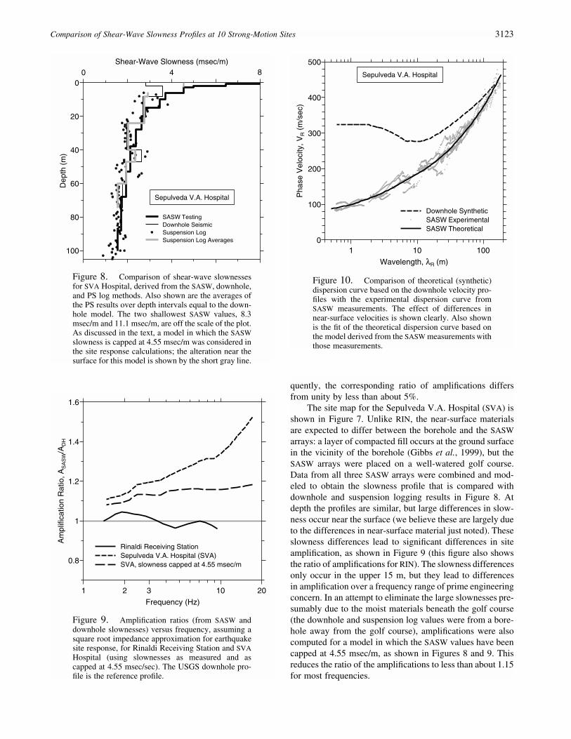
Figure 9. Amplification ratios (from SASW anddownhole slownesses) versus frequency, assuming asquare root impedance approximation for earthquakesite response, for Rinaldi Receiving Station and SVAHospital (using slownesses as measured and ascapped at 4.55 msec/sec). The USGS downhole pro-file is the reference profile.

0

20

40

60

80

100

Shear-Wave Slowness (msec/m)D

epth

(m)


Sepulveda V.A. Hospital

40 8

Figure 8. Comparison of shear-wave slownessesfor SVA Hospital, derived from the SASW, downhole,and PS log methods. Also shown are the averages ofthe PS results over depth intervals equal to the down-hole model. The two shallowest SASW values, 8.3msec/m and 11.1 msec/m, are off the scale of the plot.As discussed in the text, a model in which the SASWslowness is capped at 4.55 msec/m was considered inthe site response calculations; the alteration near thesurface for this model is shown by the short gray line.

quently, the corresponding ratio of amplifications differsfrom unity by less than about 5%.

The site map for the Sepulveda V.A. Hospital (SVA) isshown in Figure 7. Unlike RIN, the near-surface materialsare expected to differ between the borehole and the SASWarrays: a layer of compacted fill occurs at the ground surfacein the vicinity of the borehole (Gibbs et al., 1999), but theSASW arrays were placed on a well-watered golf course.Data from all three SASW arrays were combined and mod-eled to obtain the slowness profile that is compared withdownhole and suspension logging results in Figure 8. Atdepth the profiles are similar, but large differences in slow-ness occur near the surface (we believe these are largely dueto the differences in near-surface material just noted). Theseslowness differences lead to significant differences in siteamplification, as shown in Figure 9 (this figure also showsthe ratio of amplifications for RIN). The slowness differencesonly occur in the upper 15 m, but they lead to differencesin amplification over a frequency range of prime engineeringconcern. In an attempt to eliminate the large slownesses pre-sumably due to the moist materials beneath the golf course(the downhole and suspension log values were from a bore-hole away from the golf course), amplifications were alsocomputed for a model in which the SASW values have beencapped at 4.55 msec/m, as shown in Figures 8 and 9. Thisreduces the ratio of the amplifications to less than about 1.15for most frequencies.

1 10 1000

100

200

300

400

500

Wavelength, R (m)

Pha

seV

eloc

ity,V

R(m

/sec

)

Downhole SyntheticSASW ExperimentalSASW Theoretical


Figure 10. Comparison of theoretical (synthetic)dispersion curve based on the downhole velocity pro-files with the experimental dispersion curve fromSASW measurements. The effect of differences innear-surface velocities is shown clearly. Also shownis the fit of the theoretical dispersion curve based onthe model derived from the SASW measurements withthose measurements.


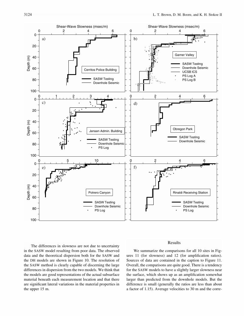
The differences in slowness are not due to uncertaintyin the SASW model resulting from poor data. The observeddata and the theoretical dispersion both for the SASW andthe DH models are shown in Figure 10. The resolution ofthe SASW method is clearly capable of discerning the largedifferences in dispersion from the two models. We think thatthe models are good representations of the actual subsurfacematerial beneath each measurement location and that thereare significant lateral variations in the material properties inthe upper 15 m.

Results

We summarize the comparisons for all 10 sites in Fig-ures 11 (for slowness) and 12 (for amplification ratios).Sources of data are contained in the caption to Figure 11.Overall, the comparisons are quite good. There is a tendencyfor the SASW models to have a slightly larger slowness nearthe surface, which shows up as an amplification somewhatlarger than predicted from the downhole models. But thedifference is small (generally the ratios are less than abouta factor of 1.15). Average velocities to 30 m and the corre-

0 2 4 60

20

40

60

80

100


epth

(m)

SASW TestingDownhole Seismic

a)

Cerritos Police Building

0 2 4 6Shear-Wave Slowness (msec/m)

SASW TestingDownhole SeismicUCSB ICSPS Log APS Log B

b)

Garner Valley

0 1 2 3 40

20

40

60

80

100

Dep

th(m

)

SASW TestingDownhole SeismicPS Log

c)

Jensen Admin. Building

0 2 4 6


d)

Obregon Park

0 5 100

20

40

60

80

100

Dep

th(m

)


e)

Potrero Canyon

0 2 4 6


f)



sponding NEHRP site classes are given in Table 1. The av-erage velocities are quite similar, but because a few are closeto the site class C-D boundary (360 m/sec), three out of theten sites have differences in the NEHRP site classes. We thinkthat this illustrates the problematical nature of site class def-initions when the average velocities are close to a classboundary rather than a limitation with the average velocitiesdetermined from SASW models; histograms of average ve-locities for extensive datasets show no indication of the classboundaries (e.g., Boore and Joyner, 1997; Wills et al., 2000).

Part of the difference between the slowness profilesfrom downhole and SASW testing is due to the different layerinterfaces. Layer intervals for the downhole profile were se-lected based on observed travel times and the borehole li-thology log, whereas no site information was used in theSASW analysis. Lateral variability may also contribute to

differences in shear-wave slowness. The downhole profile isalmost a point measurement of the subsurface properties,whereas the SASW method averages properties over hori-zontal distances related to the array length. In many geologicenvironments there may be significant changes in the sub-surface properties over the lateral dimensions averaged inthe SASW method (this is especially true in the very near-surface materials), and therefore the slowness profiles for thetwo methods, although different, might accurately reflect thesubsurface properties. In addition, neither method accountsfor anisotropy, and at some of the sites the waves beingmeasured by the SASW method may contain phases otherthan the fundamental mode Rayleigh wave.

As discussed in the introduction, the initial analysis ofthe SASW data assumed a Poisson’s ratio of 0.25, whereasthe analysis used for this article made use of the depth to the

0 2 4 60

20

40

60

80

100


epth

(m)


g)

Sylmar Converter East

0 2 4 6 8

Shear-Wave Slowness (msec/m)


h)

Sylmar Converter West

0 2 4 60

20

40

60

80

100

Dep

th(m

)


i)

Sherman Oaks Park

0 2 4 6 8 10 12


j)


Figure 11. Shear-wave slownesses at all sites, derived from the SASW, downhole,and PS logging methods. Downhole models for Rinaldi Receiving Station, SepulvedaVA Hospital, Sherman Oaks Park, Sylmar Converter West, and Jensen AdministrationBuilding) are from Gibbs et al. (1999); models for Potrero Canyon, Sylmar ConverterEast, and Obregon Park are from Gibbs et al. (2000); models for Garner Valley arefrom a revision by the second author of Gibbs (1989); and models for Cerritos CollegePolice Building are from Gibbs et al. (2001). Suspension logging models from theResolution of Site Response Issues from the Northridge Earthquake (ROSRINE) website (http://geoinfo.usc.edu/rosrine/). The UCSB ICS model for Garner Valley was basedon suspension logging results and is published in Steidl et al. (1998).


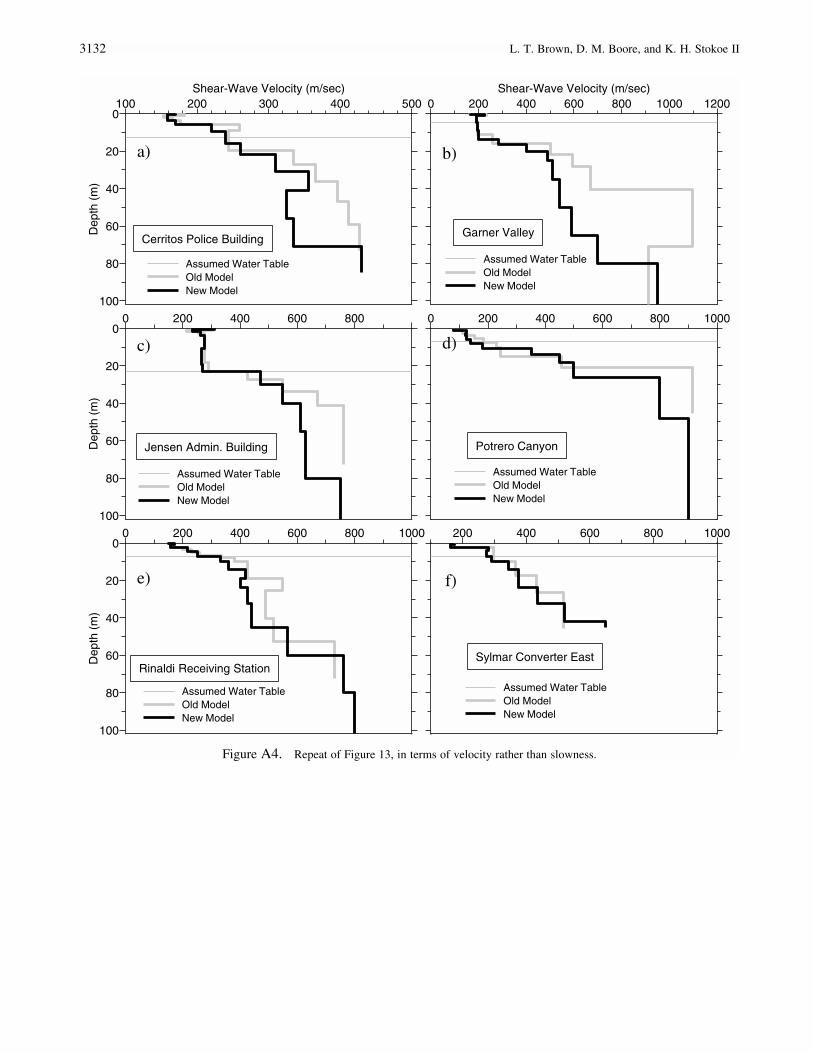
water table. A comparison of slowness for the two sets ofmodels is given in Figure 13. As expected, the largest dif-ferences are at depths below the water table, where the ear-lier assumption about Poisson’s ratio is very poor. As a resultof the change in Poisson’s ratio, the slownesses of the Swaves are generally higher (the velocities are lower) than inthe initial analysis. This is a consequence of the assumptionthat the P-wave slownesses were overestimated in the initialanalysis, leading to an underestimation of the S-wave slow-nesses as a compensation (recall that the same dispersioncurve is being matched by the old and the new models).

Conclusions

The SASW method offers the potential of evaluatingshear-wave slowness profiles quickly and at relatively smallcost. The comparison of slowness profiles from downholeseismic and SASW testing at 10 sites is generally good. Thisstudy demonstrates that in many situations the SASW methodcan provide slowness profiles suitable for site response pre-dictions. Details of the layering are less important than theaverage depth dependence of the slowness. The differencesin predicted ground-motion amplification between the slow-ness profiles from SASW and downhole testing are less than

1 2 3 10 20

0.8

1

1.2

1.4

Am

plifi

catio

nR

atio

(SA

SW

/DH

)

a) Cerritos Police Building

1 2 3 10 20

b) Garner Valley

1 2 3 10 20

0.8

1

1.2

1.4

Am

plifi

catio

nR

atio

(SA

SW

/DH

)

c) Jensen Admin. Building

1 2 3 10 20

d) Obregon Park

1 2 3 10 20

0.8

1

1.2

1.4

Am

plifi

catio

nR

atio

(SA

SW

/DH

)

e) Potrero Canyon

1 2 3 10 20

f)Rinaldi Receiving Station

1 2 3 10 20

0.8

1

1.2

1.4

Am

plifi

catio

nR

atio

(SA

SW

/DH

)

g) Sylmar Converter East

1 2 3 10 20

h) Sylmar Converter West

1 2 3 10 20

0.8

1

1.2

1.4

Frequency (Hz).

Am

plifi

catio

nR

atio

(SA

SW

/DH

)

i) Sherman Oaks Park

1 2 3 10 20Frequency (Hz).

j) Sepulveda V.A. Hospital

Figure 12. Ratio of square-root impedance amplifications from the SASW anddownhole models for all sites.


about 15% for most frequencies, which is a minor difference.SASW measurements are inherently different from bore-

hole measurements since they average material propertiesover a much larger area. Lateral variations and inhomoge-neities in the subsurface materials may cause differences inthe slowness profiles from the two methods, with the inter-esting point being that both sets of measurements may cor-rectly represent the material that has been sampled. Back-ground information such as the approximate stratigraphy and

depth to the groundwater table should be used in the SASWanalysis for greater accuracy. At sites where there is a grad-ual increase in shear stiffness with depth, the fundamental-mode Rayleigh-wave dispersion model is a good approxi-mation of the SASW experiment. At more complicated sites,surface-wave dispersion models that take into account re-ceiver geometry, body-wave energy, and higher modes ofRayleigh-wave propagation may generally improve the so-lution.

2 3 4 5 6 70

20

40

60

80

100


epth

(m)

Assumed Water TableOld ModelNew Model

a)


0 2 4 6Shear-Wave Slowness (msec/m)


b)

Garner Valley

0 1 2 3 40

20

40

60

80

100

Dep

th(m

)


c)


0 5 10 15


d)

Potrero Canyon

0 2 4 60

20

40

60

80

100

Dep

th(m

)


e)


1 2 3 4 5 6 7


f)


Figure 13. Comparison of shear-wave slownesses for model constructed assuminga constant Poisson’s ratio (old model) and for model in which the water table was takeninto account (see text) (new model). The assumed depth to the water table is shownby the horizontal line in each figure. (Continued on next page.)


0 2 4 60

20

40

60

80

100


epth

(m)


g)


0 1 2 3 4 5 6Shear-Wave Slowness (msec/m)


h)

Sherman Oaks Park

0 2 4 6 8 10 120

20

40

60

80

100

Dep

th(m

)

Assumed Water Table > 75 mOld ModelNew Model

i)


Figure 13. (Continued)

Acknowledgments

We thank numerous individuals who made it possible to obtain thefield measurements. This includes Craig Davis and Ron Tognazzini of theLos Angeles Department of Water and Power (LADWP) for access to sta-tions JMB, RIN, SCE, and SCW; University of Texas students Brent Rosen-blad and James Bay, who oversaw collection of the field data and assistedin initial SASW data reduction; Jamie Steidl for information and access tothe GV site; the ROSRINE group and Rob Stellar in particular for the PS logdata and interpretations; Jeff Owen of LADWP for onsite guidance at RIN,

SCE, and SCW; SECO for a great vibroseis crew; and the many unnamedproperty owners and managers for permission to conduct the surveys ontheir land. We’d also like to thank Jim Gibbs, Rob Kayen, and Glenn Rixfor reviews and Bob Simons of Cohort Software for help with the software(CoPlot) used to produce the figures. This work was partially supported byGrant No. 1434-HQ-97-03060 from the U.S. Geological Survey.

References

Boore, D. M. (2003). Prediction of ground motion using the stochasticmethod, Pure Appl. Geophy. 160 (in press).

Boore, D. M., and L. T. Brown (1998a). Comparing shear-wave velocityprofiles from inversion of surface-wave phase velocities with down-hole measurements: systematic differences between the CXW methodand downhole measurements at six USC strong-motion sites, Seism.Res. Lett. 69, 222–229.

Boore, D. M., and L. T. Brown (1998b). Erratum to “Comparing shear-wave velocity profiles from inversion of surface-wave phase veloci-ties with downhole measurements: systematic differences between theCXW method and downhole measurements at six USC strong-motionsites,” Seism. Res. Lett. 69, 406.

Boore, D. M., and W. B. Joyner (1997). Site amplifications for generic rocksites, Bull. Seism. Soc. Am. 87, 327–341.

Brown, L. T. (1998). Comparison of VS profiles from SASW and boreholemeasurements at strong motion sites in Southern California, M.S.Thesis, University of Texas at Austin.

Gibbs, J. F. (1989). Near-surface P- and S-wave velocities from boreholemeasurements near Lake Hemet, California, U.S. Geol. Surv. Open-File Rept. 89-630.

Gibbs, J. F., D. M. Boore, J. C. Tinsley, and C. S. Mueller (2001). BoreholeP-and S-wave velocity at thirteen stations in southern California, U.S.Geol. Surv. Open-File Rept. OF 01-506, 117 pp.

Gibbs, J. F., J. C. Tinsley, D. M. Boore, and W. B. Joyner (1999). Seismicvelocities and geological conditions at twelve sites subjected to strongground motion in the 1994 Northridge, California, earthquake: a re-vision of OFR 96-740, U.S. Geol. Surv. Open-File Rept. 99-446,142 pp.

Gibbs, J. F., J. C. Tinsley, D. M. Boore, and W. B. Joyner (2000). Boreholevelocity measurements and geological conditions at thirteen sites inthe Los Angeles, California region, U.S. Geol. Surv. Open-File Rept.OF 00-470, 118 pp.

Horike, M. (1985). Inversion of phase velocity of long-period microtremor


0 200 400 600 800 10000

20

40

60

80

100

Shear-Wave Velocity (m/sec)

Dep

th(m

)



Figure A1. Repeat of Figure 6, in terms of veloc-ity rather than slowness.

0 200 400 600 800 10000

20

40

60

80

100


Dep

th(m

)



Figure A2. Repeat of Figure 8, in terms of veloc-ity rather than slowness.

to the S-wave-velocity structure down to the basement in urbanizedareas, J. Phys. Earth 33, 59–96.

Joh, S.-H. (1992). User’s Guide to WinSASW: Data Reduction and AnalysisProgram for Spectral Analysis of Surface Waves (SASW), Universityof Texas at Austin, 51 pp.

Joh, S.-H. (1997). Advances in interpretation and analysis techniques forspectral-analysis-of-surface-waves (SASW) measurements, Ph.D. Dis-sertation, University of Texas at Austin.

Nazarian, S., and K. H. Stokoe II (1984). In situ shear wave velocities fromSpectral Analysis of Surface Waves, in Proceedings of the EighthWorld Conference on Earthquake Engineering, Prentice-Hall, Inc., En-glewood Cliffs, New Jersey, Vol. III, 31–38.

Nigbor, R. L., and T. Imai (1994). The suspension P-S velocity loggingmethod, in Geophysical Characterization of Sites, Technical Com-mittee for XIII ICSMFE, A. A. Balkema, Rotterdam, The Netherlands,57–61.

Steidl, J. H., R. J. Archuleta, A. G. Tumarkin, L. F. Bonilla, and J. C. Gariel(1998). Observations and modeling of ground motion and pore pres-sure at the Garner Valley, California, test site, in The Effects of Sur-face Geology on Seismic Motion (K. Irikura, K. Kudo, H. Okada, andT. Sasatani, Eds.), A. A. Balkema, Rotterdam, The Netherlands, Vol.1, 225–232.

Stokoe, K. H. II, G. L. Rix, and S. Nazarian (1989). In situ seismic testingwith surface waves, in Proceedings of the Twelfth International Con-ference on Soil Mechanics and Foundation Engineering, Rio de Ja-neiro, Brazil, Vol. 1, 330–334.

Stokoe, K. H., II, S. G. Wright, J. A. Bay, and J. A. Roesset (1994). Char-acterization of geotechnical sites by SASW method, in GeophysicalCharacterization of Sites, Technical Committee for XIII ICSMFE,A. A. Balkema, Rotterdam, The Netherlands, 785–816.

Wills, C. J., M. Petersen, W. A. Bryant, M. Reichle, G. J. Saucedo, S. Tan,G. Taylor, and J. Treiman (2000). A site-conditions map for Californiabased on geology and shear-wave velocity, Bull. Seism. Soc. Am. 90,S187–S208.

Zywicki, D. J. (1999). Advanced signal processing methods applied to en-gineering analysis of seismic surface waves, Ph.D. Dissertation, De-partment of Civil Engineering, Georgia Institute of Technology.

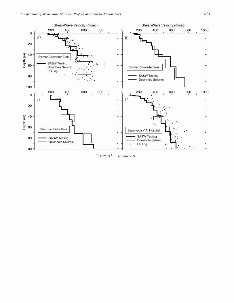
Appendix A

Figures in Terms of Velocity Rather than Slowness

Presented here are the equivalents of Figures 6, 8, 11,and 13, but using velocity rather than slowness for the ab-scissa.

U.S. Geological Survey345 Middlefield Rd., MS 977Menlo Park, California [email protected]

(D.M.B., L.T.B.)

Department of Civil EngineeringErnest Cockrell Jr. Bldg. 9.227University of Texas at AustinAustin, Texas [email protected]

(L.T.B., K.H.S.)

Manuscript received 18 January 2002.


0 100 200 300 400 5000

20

40

60

80

100

Shear-Wave Velocity (m/sec)D

epth

(m)


a)


0 500 1000 1500 2000Shear-Wave Velocity (m/sec)

SASW TestingDownhole SeismicUCSB ICSPS Log APS Log B

b)Garner Valley

0 200 400 600 8000

20

40

60

80

100

Dep

th(m

)


c)


0 200 400 600 800 1000


d)

Obregon Park

0 200 400 600 8000

20

40

60

80

100

Dep

th(m

)


e)

Potrero Canyon

0 200 400 600 800 1000


f)


Figure A3. Repeat of Figure 11, in terms of velocity rather than slowness.


0 200 400 600 8000

20

40

60

80

100


epth

(m)


g)


0 200 400 600 800 1000



h)


0 200 400 600 8000

20

40

60

80

100

Dep

th(m

)


i)

Sherman Oaks Park

0 200 400 600 800 1000


j)


Figure A3. (Continued)


100 200 300 400 5000

20

40

60

80

100


epth

(m)


a)


0 200 400 600 800 1000 1200Shear-Wave Velocity (m/sec)


b)

Garner Valley

0 200 400 600 8000

20

40

60

80

100

Dep

th(m

)


c)


0 200 400 600 800 1000


d)

Potrero Canyon

0 200 400 600 800 10000

20

40

60

80

100

Dep

th(m

)


e)


200 400 600 800 1000


f)


Figure A4. Repeat of Figure 13, in terms of velocity rather than slowness.


0 200 400 600 8000

20

40

60

80

100


epth

(m)


g)


0 200 400 600 800 1000Shear-Wave Velocity (m/sec)


h)

Sherman Oaks Park

0 200 400 600 800 10000

20

40

60

80

100

Dep

th(m

)

Assumed Water Table > 75 mOld ModelNew Model

i) Sepulveda V.A. Hospital

Figure A4. (Continued)

comparison of shear-wave slowness proﬁles at 10 · pdf filecomparison of shear-wave slowness...

Documents