1

Citation: Cheng, N. S., Hao, Z. Y., and Tan, S. K. (2008). “Comparison of quadratic and power law for nonlinear flow through porous media.” Experimental Thermal Fluid Science, 32(8), 1538-1547.

Comparison of Quadratic and Power Law for Nonlinear Flow through Porous Media

Nian-Sheng Cheng, Zhiyong Hao, and Soon Keat Tan

School of Civil and Environmental Engineering Nanyang Technological University, Singapore 639798

Tel: 65-6790 6936; Fax: 65-6791 0676; Email: cnscheng@ntu.edu.sg ___________________________________________________________________________

Abstract: The quadratic and power laws are two typical formulations that can be used to

extend the Darcy law to non-Darcy flows through porous media. Both laws are reformulated

in the dimensionless form in this study. They are then evaluated by fitting to experimental

data with specified variations in seepage velocity, which were specifically collected for a

simplified ordered porous model. The results show that the quadratic law is applicable to both

linear and nonlinear flow regimes but the two coefficients vary at different regimes. In

comparison, the power law appears not workable if the seepage velocity varies over a wide

range. This study also demonstrates that the two parameters included in the power law are

generally interrelated, and the relationship derived based on the quadratic law compares well

with the experimental results. To help understand the non-linear behavior associated with the

simplified porous model, CFD simulations were also performed to visualize and elucidate

localized 3D flow phenomena.

Keywords: Porous media; Darcy law; Inertial effect; Turbulence; Nonlinear flow; Seepage;

Power law; Groundwater

___________________________________________________________________________

2

1. Introduction

Non-Darcy flows take place at relatively high seepage velocity through porous media such as

rockfills, gravel beds and waste dumps. Modelling of such flows is often required in many

disciplines including groundwater, geotechnical and environmental engineering. Empirical

and theoretical efforts have been made in past decades to extend the Darcy law to the flow

through porous media with significant inertial effects. For engineering applications, several

formulations of flow resistance have been proposed (Kovács 1981), of which the most typical

examples are the quadratic and power models given in the following form:

2sss buaui += (1)

mss cui = (2)

where is = hydraulic gradient; us = bulk or superficial seepage velocity; a, b and c =

coefficients; and m = power varying from 1 to 2. The four parameters (a, b, c and m) can be

evaluated from experimental data.

Eq. (1) is also called Forchheimer equation (Bear 1988). It was proposed on the

grounds that the seepage-related energy dissipation is taken as a sum of energy losses

associated with viscous drag and inertial effects. For the case of creeping flow, the viscous

drag is linear and thus the Darcy law prevails, as is represented by the first term on the right-

hand-side of Eq. (1). With increasing seepage velocity, deviation from the Darcy law takes

place because of flow separation at the lee of particles and/or the onset of turbulence. The

deviation, in spite of its origins, finally results in a nonlinear drag, which can be well

approximated as a function that is proportional to the squared seepage velocity as given by

the second term on the right-hand-side of Eq. (1). Some theoretical attempts have been

devoted to associate the nonlinear drag with inertial and/or turbulent effects of viscous flow;

relevant pioneering references includes Mei and Auriault (1991), Skjetne and Auriault

3

(1999), and Wodie and Levy (1991). However, the theoretical bases of these attempts are still

controversial in the literature (e.g. Bear 1988). Direct numerical simulation appears recently

as a practical alternative to visualise the transition of flow from linear to nonlinear behaviour.

For example, by solving the Navier-Stokes equations for a two-dimensional disordered

porous structure with high porosity, Andrade (1999) demonstrated that the incipient departure

from the Darcy law that is in agreement with Eq. (1) can be observed in the laminar regime of

fluid flow without including turbulence effects.

In comparison with Eq. (1), the power form [Eq. (2)] also works well, sometimes even

better, in representing variations in the pressure drop measured for different seepage

velocities (Bordier and Zimmer 2000; Trussell and Chang 1999). Cheng and Chiew (1999)

reported that from data-fitting performed for the entire range of the seepage velocity, which

was observed through porous column comprising sand or gravel, the estimated power (m)

increased with the dimensionless pore length scale.

Although the quadratic law could be somehow derived from the Navier-Stokes

equations with certain arguments (Chen et al. 2001), both types of functions are often

employed to empirically present data-based correlations. This is because it is still generally

unclear that to what content these functions are able to characterize reasonably the physics

inherent in the flow phenomena. Other questions worthy of further theoretical efforts include

under what conditions the nonlinear term appears, and the viscous drag becomes proportional

to the squared seepage velocity. Qualitatively, the above questions about seepage flow may

be understood by making an analogy with flow around a spherical object. For the latter case,

flow separation behind a particle can occur even prior to the onset of turbulence (van Dyke

1982), which explains the deviation of the settling drag from the linear Stokes regime.

On the other hand, for engineering applications, it would be very interesting to

understand how the two laws differ from each other because one form of function may be

4

preferred to the other. Some analyses in this respect have been presented, for example, by

George and Hansen (1992) and Niven (2000). George and Hansen (1992) theoretically

showed that the data-based conversions between the two laws are always possible, but the

coefficients estimated from one pair to another (i.e. from a and b to c and m, or from c and m

to a and b) is subject to the maximum seepage velocity under consideration. Another

conversion study is due to Niven (2000), who first numerically generated a database of the

hydraulic gradient with the quadratic function and then fitted to the power function. The

results so obtained show that the power law was able to predict the hydraulic gradient within

an error of 22%.

In this study, seepage was observed through a laboratory experiment designed with a

simplified ordered porous media model. The functional relation of flow resistance is

presented on the grounds of dimensional analysis in terms of the friction factor and Reynolds

number. The measured results are then fitted to the quadratic and power functions and the

variations associated with the parameters included in the functions are examined in detail. In

addition, numerical simulations were also conducted to help appreciate relevant micro-flow

phenomena localised in the pore domain.

2. Laboratory experiment with ordered porous model

The porous media employed in the experiment were modelled by placing glass beads into a

square steel pipe of 3 m in length. The diameter of the glass bead, D, was 16 mm and the

cross section of the pipe was measured as l2 = 16.4 × 16.4 mm2. The beads were packed

closely along the pipe and the bead-to-bead gap was not allowed. However, the movement of

beads in the transverse direction was possible because of the small difference (0.4 mm gap)

between the bead size and the cross-section dimension, but its effect is considered

5

insignificant. The resulted global porosity was 0.50 and the cross-sectional porosity varied

from 1 to 0.25 because of a gradual increase in the cross-sectional area of the flow passage

(Ap) from the largest blockage (x/D = 0) to the zero blockage (x/D = 0.5), where x is a

longitudinal distance measured from the centre of a glass bead. The variation of Ap with x for

0 ≤ x ≤ D/2 is given by

⎟⎟⎠

⎞⎜⎜⎝

⎛−−= 2

2

2

2

2 41

lx

lD

lAP π (3)

This simplified model is free of irregularities induced by random granular configuration and

also facilitates control of flows. In addition, it would be possible to explore details of fluid

flowing in the pores with the aid of computational hydrodynamic technique. As shown later

in this paper, the results obtained differ quantitatively from those available in the literature

for conventional porous media with random configuration. However, they provide an

alternative insight into the transition between the linear and non-linear flow domains, and

also a well-defined physical model for assessing how well the transition can be described

with the quadratic and power functions.

To have a wide range of the Reynolds number, both clear water and water-glycerine

mixture were used as the fluid media. The viscosity of the mixture which varied with

temperature was measured using a piston-type viscometer manufactured by Cambridge

Applied Systems. A few probes applied for different ranges of viscosities were employed.

The temperature-dependence of viscosity was first calibrated for a range of temperatures and

also fitted empirically using exponential functions. The so-obtained calibration curves were

then applied to test cases with individual temperatures taken. The pipe flow was driven using

a submergible pump. The error in measuring the pressure drop was less than 2% either using

a water-based manometer or mercury-based manometer.

Altogether four series of experiments comprising 242 runs were completed. The test

6

conditions are summarized in Table 1. Four kinds of fluids (G00, G50, G70, and G80) were

prepared by setting the concentration of glycerine roughly at 0%, 50%, 67% and 80%,

respectively. The use of the low-molecular weight fluids, glycerine and its aqueous solutions,

implies that the experiments done were under the condition of Newtonian fluids. The

variations of the hydraulic gradient with the seepage velocity are plotted in Fig. 1. The

average flow velocity varied from 0.004 to 0.282 m/s. The use of glycerine-water mixture

made available a range of fluid kinematic viscosity (ν) from 0.7 to 35 cSt (10-6 m2/s). As a

result, the Reynolds number (= usD/ν) varied from 2 to 5550, where us is the superficial

seepage velocity and D is the bead diameter. The observed flows covered the Darcy-type

linear regime and also inertia-dominant nonlinear regime.

3. Dimensional Analysis

Resistance of flows through porous media can be investigated by making an analogy with

that considered in conventional pipe flows because both flows are boundary-confined.

Several attempts in this respect have been reported in literature (Bear 1988), which involve

various geometric simplifications of porous media. These are not replicated in this study.

Instead, the consideration presented here only engages two parameters, friction factor and

Reynolds number. By drawing an analogy with pipe flows, these two parameters can be

redefined by including effects of porous media, so that the flow resistance relationship can be

presented in a way similar to the Moody diagram, which is often included in fluid mechanics

books.

Here, we use fp and Rep to denote the friction factor and Reynolds number for pipe

flows, respectively. The relation of fp-Rep varies generally with the relative roughness length,

but becomes unique for hydrodynamically smooth pipes. In this study, it is assumed that the

7

boundary of interstitial flows is hydrodynamically smooth so that the roughness effect is

ignored. This is acceptable by noting the experimental condition described in the previous

section. By definition, fp is proportional to (u∗p/Up)2 and Rep = UpRp/ν, where u∗p = (gRpip)0.5,

Rp = hydraulic radius, Up is the average velocity through the pipe, ν = kinematic viscosity of

fluid, ip = hydraulic gradient and g = gravitational acceleration.

In the following, both fp and Rep are modified to apply for the case of the interstitial

flow in porous media. Being differentiated from the parameters used for pipe flows, those

related to seepage flow are denoted with the subscript, s. First, the average velocity Us is

computed with respect to the pore space. If the average porosity is ε, Us is given by

ε= s

suU (4)

where us is the bulk or superficial seepage velocity, which is the volumetric flux of fluid per

unit area (computed in the spatial domain composed of pores and particle matrix).

Second, the hydraulic radius Rp can be replaced with Rs, the characteristic length of

the cross-sectional area of the flow. The latter can be shown to be proportional to the particle

size for porous media. For a one-dimensional flow, Rp is defined as the ratio of the cross-

sectional area to the wetted perimeter of the flow. This concept can be further extended to the

three-dimensional space by defining the hydraulic radius as the ratio of the volume of the

interstitial space to the area of the interface between solid and fluid. Consider a porous media

of a unit volume. The total volume of the pores within this volume is ε. If the particle

diameter is D, the number of the particles enclosed is (1- ε)/(πD3/6) and the total interfacial

area is equal to πD2(1-ε)/(πD3/6) = 6(1- ε)/D. Then, by ignoring the constant coefficient, the

redefined hydraulic radius Rs is proportional to the particle size D, i.e.

DRs ε−ε

=1

(5)

8

It is noted that the dimensionless pore scale can be defined as (g/ν2)1/3 Rs (Cheng 2003). With

the modified hydraulic radius, the seepage shear velocity can be expressed as

ssss gDiigRuε

ε−

==1* (6)

As a result, the flow resistance relation of fp-Rep is revised in the form of fs-Res, where fs is

the seepage friction factor defined as

2

32

*

1 s

s

s

ss u

gDiUuf

ε−ε

=⎟⎟⎠

⎞⎜⎜⎝

⎛= (7)

and Res is the seepage Reynolds number given by

νενDuRURe sss

s −==

11 (8)

Approximately, Res can be understood as a measure of the ratio of inertial to viscous effect in

a ‘simplified’ pipe flow that represents the porous media.

Since the hydraulic gradient is is proportional to the squared shear velocity, 2*su , the

empirical quadratic and power functions, Eqs. (1) and (2), can be re-written respectively in

the following dimensionless form:

22* ⎟

⎠⎞

⎜⎝⎛

ν+⎟

⎠⎞

⎜⎝⎛

ν=⎟

⎠⎞

⎜⎝⎛

νssssss RuBRuARu or 22

* sss BReAReRe += (9)

Mssss RuCRu

⎟⎠⎞

⎜⎝⎛

ν=⎟

⎠⎞

⎜⎝⎛

ν

2* or M

ss CReRe =2* (10)

where Re∗s = u∗sRs/ν = seepage-related shear Reynolds number; A, B and C = coefficients;

and M = exponent. It is noted that in performing the above dimensional transformation, only

the characteristic pore scale and kinematic viscosity of fluid are used. It should also be

mentioned that the relation given by Eq. (9) actually follows the same form of the Ergun

equation (Bear 1988; Cheng 2003),

9

( ) 2332

2 175.11150 sss ugD

ugD

iεε

εεν −

+−

= (11)

which suggests that on average, A = 150 and B = 1.75 for natural porous media. These two

average values would vary for other artificial porous media, as exemplified later by this

study.

4. Comparison of quadratic and power laws

In the subsequent analysis, the experimental data will be used to explore variations in the four

parameters, i.e. the three coefficients (A, B and C) and power (M) included in Eqs. (9) and

(10) rather than those initially given in Eqs. (1) and (2).

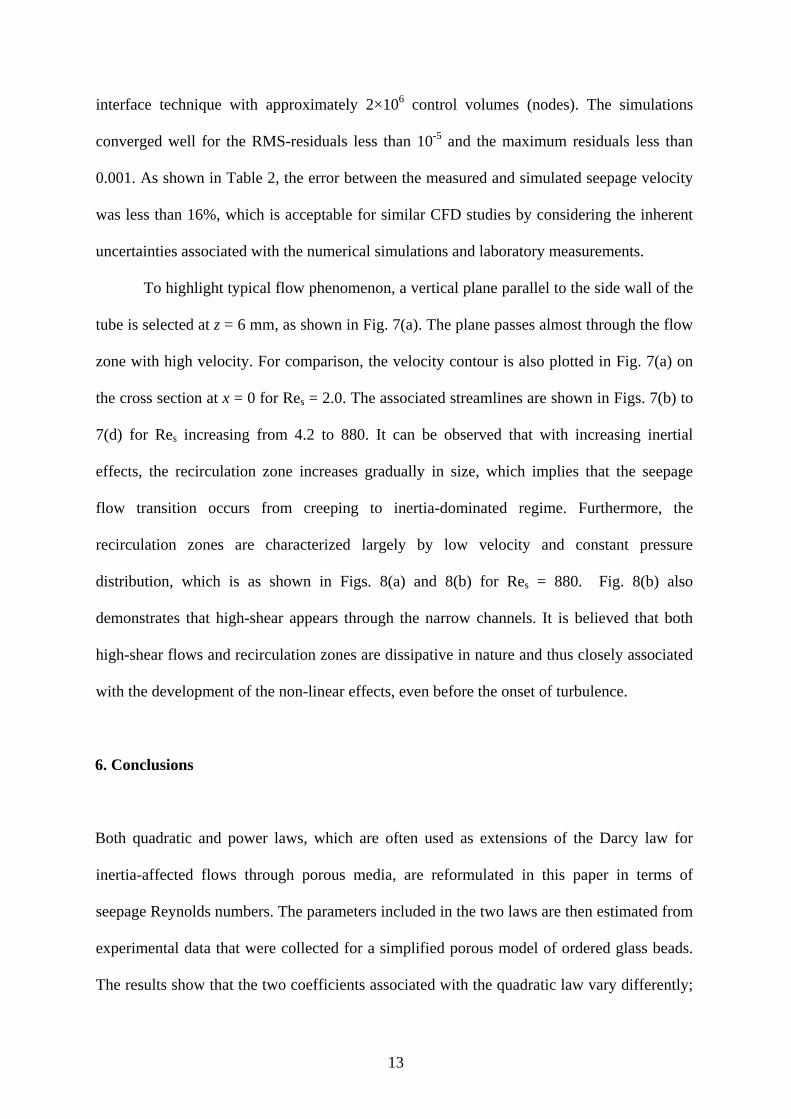
First, we combine all data series in terms of the two dimensionless parameters, Re*s

and Res. By plotting Re 2*s against Res, it is found the data points collected for the different

runs collapsed almost into a single curve, as shown in Fig. 2. Also superimposed in the figure

are two asymptotes, Re 2*s = 674Res and Re 2

*s = 0.95Res2, for very small and large Reynolds

numbers, respectively. Second, to fit the data to the proposed empirical functions, Eqs. (9)

and (10), the combined data series are further sorted according to ascending Res-values. As

expected, the optimised values for A, B, C and M depend on the range of data selected for the

best-fit. To avoid any deviation induced by any subjective data selection, the sorted data

series is then divided into eleven subsets and the adjacent two subsets are allowed to overlap

by 50%. Next, for each subset of data, the best-fit is then performed and the corresponding

values of A, B, C and M are calculated. The results so obtained are plotted in Figs. 3 and 4,

where the middle value of the seepage Reynolds number for each subset is used. It is

interesting to note that all four parameters are not constant, generally varying with the

10

seepage Reynolds number (Res), and in particular, the variations associated with C and M are

more appreciable.

Fig. 3 shows that the estimated A-value appears to be a constant at low Reynolds

numbers but fluctuates at high Reynolds numbers. The opposite scenario holds for the

estimated B-values. Such variations are understandable by noting that the linear term

included in the quadratic model is dominant only for small Reynolds numbers and the

nonlinear contribution becomes more important for high Reynolds numbers. On the other

hand, the variations in A and B, which are not small, imply that the quadratic law could not

represent exactly the characteristics of porous media flows. In spite of the fact that the

variations in A and B may be subject to the data accuracy to certain extent, the observation is

not consistent with theoretical attempts that favour the quadratic law.

The result presented in Fig. 4, despite the scattering data points, clearly demonstrates

that both C and M vary to a great extent with the Reynolds number. This is somehow not

consistent with the assumption made implicitly in performing data-fit with the power model.

The significant variation of C (or M) with the Reynolds number means that a single value of

C (or M) is not attainable in principle for seepage flow with varying velocities for a given

porous medium.

A further inspection of Fig. 4 indicates that with increasing Reynolds number or

inertial effect, the C-value reduces from A to B (i.e. B ≤ C ≤ A) while the M-value increases

from 1 to 2 (i.e. 1 ≤ M ≤ 2). This suggests that a possible correlation would exist among the

four parameters, for example, between the two ratios, (A-C)/(C-B) and (2-M)/(M-1), as shown

in Fig. 5.

From the above data-fit exercise, it is observed that the quadratic model is generally

applicable in spite of the variations in the two coefficients. In contrast, the power model may

approximate well the measurements of the pressure drop provided only that the range of

11

seepage velocity under consideration is not large. This is because both the coefficient and

power included in the power model are very sensitive to the seepage Reynolds number.

If the prediction by the quadratic model is assumed to be exact, the two parameters, C

and M, can be theoretically interrelated. This can be shown by considering the following two

equations, which are the simplified versions of Eqs. (9) and (10) used for data-fitting,

21 BxAxy += (12)

MCxy =2 (13)

To determine the relationship among the coefficients (A, B and C) and power (M), we first

assume that y1 ≈ y2 for any x, which yields

1−=+ MCxBxA (14)

Then, let dy1/dx ≈ dy2/dx, one gets

12 −=+ MCMxBxA (15)

Solving Eqs. (14) and (15) for x,

MM

BAx

−−

=2

1 (16)

Substituting Eq. (16) into Eq. (14) gives

M

MM

BA

MBC

−

⎟⎠⎞

⎜⎝⎛

−−

−=

2

21

1 (17)

From Eq. (17), it follows that as expected, C varies between A and B, approaching A as M →

1 and B as M → 2. Using Eq. (17), C can be estimated directly for M varying within a

limited range for a given dataset, and vice versa. The results computed with Eq. (17) are

plotted in Fig. 6, showing that it gives a good representation of the relation among the

estimated parameters. Here the values of A and B are taken as 976 and 1.0, respectively,

which are obtained by fitting Eq. (9) to the entire dataset.

12

5. Discussions

Various artificial porous media models have been used in previous studies, many being

designed for numerical simulations and only a few for laboratory investigations. In light of

the studies summarised by Hlushkou and Tallarek (2006), the seepage flow investigated in

this study would remain to be Darcian for Res < 5.4 (inertial contribution ≈ 5%), laminar for

Res < 240 (inertial contribution ≈ 70%); and turn to be turbulent for Res > 1200 (inertial

contribution ≈ 90%). These critical values are generally in good agreement with the results

shown in Fig. 2.

The present porous media model could be evaluated in terms of the permeability (K),

which is related to A in Eq. (9) in the form of K = D2ε3/[A(1-ε)2]. The best fit of the

experimental data to the quadratic law gives A = 976. With D = 16mm and ε = 0.5, we get K

= 1.3 × 10-7 m2. For comparison, an empirical formula given on Page 132 in Bear (1988) is

also used, i.e. K = 0.617 × 10-11D2, where K is in cm2 and D is in microns. With D = 16000

microns, the formula yields K = 1.6 × 10-7 m2, which is very close to the experimental

measurement.

In addition to the two empirical laws, a cubic law (see Fourar et al. 2004) has been

also applied for describing the onset of the non-linear behaviour. With the data collected in

this study, best-fit exercises show that the cubic law predicts the measurements with large

deviations. For example, the average errors are 26.1%, 11.4%, 5.4% and 3.3% for Cases G00,

G50, G70 and G80, respectively. In comparison, the quadratic function yields lower errors,

which are 1.1%, 4.0%, 1.9% and 2.9%, respectively, for the four cases.

To further understand the non-linear effect, numerical simulations (11 runs in total)

were also performed to visualise micro-flow phenomena confined in the pore space. The

Navier-Stokes equations were solved using ANSYS® CFX® translational periodicity

13

interface technique with approximately 2×106 control volumes (nodes). The simulations

converged well for the RMS-residuals less than 10-5 and the maximum residuals less than

0.001. As shown in Table 2, the error between the measured and simulated seepage velocity

was less than 16%, which is acceptable for similar CFD studies by considering the inherent

uncertainties associated with the numerical simulations and laboratory measurements.

To highlight typical flow phenomenon, a vertical plane parallel to the side wall of the

tube is selected at z = 6 mm, as shown in Fig. 7(a). The plane passes almost through the flow

zone with high velocity. For comparison, the velocity contour is also plotted in Fig. 7(a) on

the cross section at x = 0 for Res = 2.0. The associated streamlines are shown in Figs. 7(b) to

7(d) for Res increasing from 4.2 to 880. It can be observed that with increasing inertial

effects, the recirculation zone increases gradually in size, which implies that the seepage

flow transition occurs from creeping to inertia-dominated regime. Furthermore, the

recirculation zones are characterized largely by low velocity and constant pressure

distribution, which is as shown in Figs. 8(a) and 8(b) for Res = 880. Fig. 8(b) also

demonstrates that high-shear appears through the narrow channels. It is believed that both

high-shear flows and recirculation zones are dissipative in nature and thus closely associated

with the development of the non-linear effects, even before the onset of turbulence.

6. Conclusions

Both quadratic and power laws, which are often used as extensions of the Darcy law for

inertia-affected flows through porous media, are reformulated in this paper in terms of

seepage Reynolds numbers. The parameters included in the two laws are then estimated from

experimental data that were collected for a simplified porous model of ordered glass beads.

The results show that the two coefficients associated with the quadratic law vary differently;

14

the coefficient used for the linear term fluctuates for large Reynolds number and that for

nonlinear term varies significantly for low Reynolds number. On the other hand, the two

parameters (i.e., the coefficient and power) included in the power law vary more

significantly and also correlate to each other. The relation among the four parameters that is

analytically derived is in good agreement with that estimated from experimental data. This

study suggests that the quadratic law generally represents well (but not exactly) the

resistance of the seepage flow including the Darcy and non-Darcy regimes, while the power

law is applicable only when the seepage velocity varies within a limited range. CFD

simulation study was also conducted to aid visualization of the flow phenomenon in the

porous medium. The simulation results show that the fluid transport in the porous model is

subject to the dissipative high-shear and pressure losses, which may explain the highly

nonlinear behaviour.

Acknowledgements

The writer gratefully acknowledges the efforts made by H. P. Liew, S. T. Soh, and M. M. Ng

for collecting the experimental data. Thanks also go to K. H. Chia and K. H. Lim for their

assistance in the experiment construction and instrument setup.

References

Andrade, J. S., Costa, U. M. S., Almeida, M. P., Makse, H. A., and Stanley, H. E. (1999). "Inertial effects on fluid flow through disordered porous media." Physical Review Letters, 82(26), 5249-5252.

Bear, J. (1988). Dynamics of fluids in porous media, Dover, New York. Bordier, C., and Zimmer, D. (2000). "Drainage equations and non-Darcian modelling in

coarse porous media or geosynthetic materials." Journal of Hydrology, 228(3-4), 174-187.

Chen, Z. X., Lyons, S. L., and Qin, G. (2001). "Derivation of the Forchheimer law via homogenization." Transport in Porous Media, 44(2), 325-335.

15

Cheng, N. S. (2003). "Application of Ergun equation to computation of critical shear velocity subject to seepage." Journal of Irrigation and Drainage Engineering-ASCE, 129(4), 278-283.

Cheng, N. S., and Chiew, Y. M. (1999). "Incipient sediment motion with upward seepage." Journal of Hydraulic Research, 37(5), 665-681.

Fourar, M., Radilla, G., Lenormand, R., and Moyne, C. (2004). "On the non-linear behavior of a laminar single-phase flow through two and three-dimensional porous media." Advances in Water Resources, 27(6), 669-677.

George, G. H., and Hansen, D. (1992). "Conversion between quadratic and power law for non-Darcy Flow." Journal of Hydraulic Engineering-ASCE, 118(5), 792-797.

Hlushkou, D., and Tallarek, U. (2006). "Transition from creeping via viscous-inertial to turbulent flow in fixed beds." Journal of Chromatography A, 1126(1-2), 70-85.

Kovács, G. (1981). Seepage hydraulics, Elsevier Scientific Pub. Co., Amsterdam ; New York.

Mei, C. C., and Auriault, J. L. (1991). "The effect of weak inertia on flow through a porous-medium." Journal of Fluid Mechanics, 222, 647-663.

Niven, R. K. (2000). "Incipient sediment motion with upward seepage - Discussion." Journal of Hydraulic Research, 38(6), 475-477.

Skjetne, E., and Auriault, J. L. (1999). "High-velocity laminar and turbulent flow in porous media." Transport in Porous Media, 36(2), 131-147.

Trussell, R. R., and Chang, M. (1999). "Review of flow through porous media as applied to head loss in water filters." Journal of Environmental Engineering-ASCE, 125(11), 998-1006.

van Dyke, M. (1982). An album of fluid motion, Parabolic Press, Stanford, Calif. Wodie, J. C., and Levy, T. (1991). "Nonlinear rectification of darcy law." Comptes Rendus

De L Academie Des Sciences Serie Ii, 312(3), 157-161.

16

Table 1. Experimental data collected for the four series.

Series G00

Run us (m/s) i ν(m2/s) Run us (m/s) i ν(m2/s) Run us (m/s) i ν(m2/s)

1 0.2817 1.898 8.1E-07 28 0.1784 0.794 8.0E-07 55 0.0883 0.215 8.3E-07

2 0.2777 1.840 8.1E-07 29 0.1721 0.752 8.0E-07 56 0.0864 0.207 8.3E-07

3 0.2754 1.814 8.1E-07 30 0.1666 0.710 8.0E-07 57 0.0855 0.201 8.3E-07

4 0.2736 1.793 8.1E-07 31 0.1607 0.664 8.0E-07 58 0.0829 0.194 8.2E-07

5 0.2704 1.760 7.9E-07 32 0.1566 0.622 8.0E-07 59 0.0803 0.181 8.2E-07

6 0.2663 1.714 7.9E-07 33 0.1547 0.605 7.8E-07 60 0.0779 0.171 8.2E-07

7 0.2629 1.672 7.9E-07 34 0.1504 0.580 7.9E-07 61 0.0743 0.158 8.2E-07

8 0.2600 1.630 7.9E-07 35 0.1464 0.546 7.9E-07 62 0.0704 0.144 8.2E-07

9 0.2547 1.588 7.9E-07 36 0.1440 0.521 7.8E-07 63 0.0668 0.130 8.1E-07

10 0.2507 1.529 7.9E-07 37 0.1402 0.512 7.9E-07 64 0.0640 0.123 8.1E-07

11 0.2474 1.470 7.9E-07 38 0.1359 0.483 7.9E-07 65 0.0613 0.114 8.1E-07

12 0.2422 1.420 7.9E-07 39 0.1319 0.454 7.9E-07 66 0.0577 0.102 8.1E-07

13 0.2410 1.399 8.1E-07 40 0.1256 0.420 7.9E-07 67 0.0546 0.095 8.1E-07

14 0.2389 1.378 8.3E-07 41 0.1188 0.378 7.9E-07 68 0.0518 0.086 8.1E-07

15 0.2347 1.327 8.3E-07 42 0.1117 0.340 7.9E-07 69 0.0484 0.076 8.0E-07

16 0.2299 1.285 8.2E-07 43 0.1072 0.311 7.8E-07 70 0.0454 0.071 8.0E-07

17 0.2263 1.243 8.2E-07 44 0.0992 0.269 7.8E-07 71 0.0426 0.062 7.9E-07

18 0.2217 1.193 8.2E-07 45 0.0934 0.244 7.8E-07 72 0.0384 0.052 7.9E-07

19 0.2163 1.151 8.2E-07 46 0.0857 0.206 7.8E-07 73 0.0352 0.044 7.9E-07

20 0.2114 1.105 8.1E-07 47 0.1050 0.298 8.5E-07 74 0.0328 0.040 7.9E-07

21 0.2083 1.079 8.1E-07 48 0.1037 0.289 8.5E-07 75 0.0305 0.036 7.9E-07

22 0.2054 1.046 8.1E-07 49 0.1011 0.279 8.5E-07 76 0.0250 0.027 7.9E-07

23 0.2029 1.012 8.1E-07 50 0.0990 0.268 8.4E-07 77 0.0214 0.022 7.8E-07

24 0.1962 0.966 8.1E-07 51 0.0956 0.252 8.4E-07 78 0.0160 0.014 7.8E-07

25 0.1919 0.928 8.1E-07 52 0.0941 0.243 8.4E-07 79 0.0130 0.011 7.8E-07

26 0.1882 0.878 8.1E-07 53 0.0922 0.235 8.4E-07 80 0.0124 0.010 7.7E-07

27 0.1839 0.836 8.0E-07 54 0.0903 0.227 8.3E-07

Series G50

81 0.2245 1.936 4.4E-06 101 0.1642 1.071 4.3E-06 121 0.0653 0.252 4.2E-06

82 0.2222 1.915 4.4E-06 102 0.1568 1.021 4.3E-06 122 0.0602 0.218 4.2E-06

83 0.2209 1.898 4.4E-06 103 0.1532 0.974 4.3E-06 123 0.0550 0.202 4.2E-06

84 0.2177 1.861 4.4E-06 104 0.1478 0.932 4.3E-06 124 0.0508 0.176 4.2E-06

85 0.2173 1.819 4.4E-06 105 0.1417 0.895 4.3E-06 125 0.0464 0.164 4.2E-06

86 0.2157 1.772 4.4E-06 106 0.1389 0.861 4.3E-06 126 0.0424 0.147 4.4E-06

87 0.2108 1.726 4.4E-06 107 0.1373 0.823 4.3E-06 127 0.0446 0.143 4.2E-06

88 0.2098 1.680 4.4E-06 108 0.1331 0.773 4.3E-06 128 0.0399 0.126 4.2E-06

89 0.2042 1.646 4.4E-06 109 0.1273 0.722 4.3E-06 129 0.0363 0.130 4.4E-06

90 0.2027 1.600 4.4E-06 110 0.1197 0.689 4.3E-06 130 0.0337 0.105 4.2E-06

91 0.1967 1.541 4.4E-06 111 0.1152 0.638 4.3E-06 131 0.0285 0.088 4.2E-06

92 0.1910 1.466 4.4E-06 112 0.1091 0.596 4.3E-06 132 0.0249 0.071 4.2E-06

93 0.1874 1.428 4.3E-06 113 0.1031 0.512 4.2E-06 133 0.0325 0.105 4.3E-06

17

94 0.1859 1.386 4.3E-06 114 0.1008 0.491 4.2E-06 134 0.0283 0.092 4.3E-06

95 0.1850 1.357 4.3E-06 115 0.0940 0.458 4.2E-06 135 0.0212 0.067 4.3E-06

96 0.1841 1.319 4.3E-06 116 0.0922 0.424 4.2E-06 136 0.0166 0.050 4.3E-06

97 0.1812 1.294 4.3E-06 117 0.0874 0.391 4.2E-06 137 0.0157 0.046 4.3E-06

98 0.1777 1.243 4.3E-06 118 0.0817 0.365 4.2E-06 138 0.0115 0.034 4.3E-06

99 0.1721 1.184 4.3E-06 119 0.0771 0.328 4.2E-06 139 0.0094 0.025 4.3E-06

100 0.1678 1.126 4.3E-06 120 0.0698 0.286 4.2E-06

Series G70

140 0.1503 1.945 1.3E-05 157 0.1079 1.159 1.2E-05 174 0.0629 0.559 1.1E-05

141 0.1484 1.898 1.3E-05 158 0.1054 1.134 1.2E-05 175 0.0587 0.525 1.1E-05

142 0.1451 1.844 1.3E-05 159 0.1033 1.084 1.2E-05 176 0.0544 0.462 1.1E-05

143 0.1428 1.798 1.3E-05 160 0.1019 1.054 1.2E-05 177 0.0490 0.420 1.1E-05

144 0.1408 1.760 1.3E-05 161 0.0981 1.008 1.2E-05 178 0.0441 0.365 1.1E-05

145 0.1380 1.676 1.2E-05 162 0.0947 0.962 1.2E-05 179 0.0410 0.323 1.1E-05

146 0.1340 1.630 1.2E-05 163 0.0922 0.924 1.2E-05 180 0.0351 0.269 1.1E-05

147 0.1319 1.592 1.2E-05 164 0.0895 0.903 1.2E-05 181 0.0306 0.235 1.1E-05

148 0.1299 1.537 1.2E-05 165 0.0872 0.848 1.2E-05 182 0.0269 0.197 1.1E-05

149 0.1295 1.512 1.2E-05 166 0.0838 0.819 1.2E-05 183 0.0227 0.160 1.1E-05

150 0.1279 1.483 1.2E-05 167 0.0835 0.790 1.2E-05 184 0.0186 0.134 1.1E-05

151 0.1251 1.445 1.2E-05 168 0.0810 0.769 1.1E-05 185 0.0162 0.105 1.1E-05

152 0.1223 1.403 1.2E-05 169 0.0786 0.748 1.1E-05 186 0.0122 0.076 1.1E-05

153 0.1205 1.352 1.2E-05 170 0.0772 0.710 1.1E-05 187 0.0092 0.055 1.1E-05

154 0.1163 1.306 1.2E-05 171 0.0754 0.693 1.1E-05 188 0.0065 0.038 1.1E-05

155 0.1151 1.256 1.2E-05 172 0.0700 0.647 1.1E-05 189 0.0042 0.025 1.1E-05

156 0.1108 1.210 1.2E-05 173 0.0672 0.613 1.1E-05

Series G80

190 0.0733 1.886 3.7E-05 208 0.0443 1.025 3.9E-05 226 0.0218 0.458 3.7E-05

191 0.0715 1.852 3.7E-05 209 0.0434 0.970 3.7E-05 227 0.0214 0.454 3.8E-05

192 0.0697 1.806 3.8E-05 210 0.0411 0.958 3.9E-05 228 0.0213 0.433 3.5E-05

193 0.0692 1.768 3.8E-05 211 0.0407 0.937 3.8E-05 229 0.0187 0.391 3.6E-05

194 0.0683 1.726 3.7E-05 212 0.0415 0.903 3.7E-05 230 0.0194 0.382 3.5E-05

195 0.0669 1.693 3.7E-05 213 0.0381 0.853 3.8E-05 231 0.0172 0.344 3.6E-05

196 0.0648 1.659 4.0E-05 214 0.0376 0.802 3.5E-05 232 0.0162 0.315 3.6E-05

197 0.0637 1.575 3.7E-05 215 0.0349 0.798 3.7E-05 233 0.0146 0.294 3.6E-05

198 0.0603 1.516 4.0E-05 216 0.0342 0.764 3.8E-05 234 0.0137 0.256 3.6E-05

199 0.0600 1.470 4.0E-05 217 0.0349 0.735 3.5E-05 235 0.0123 0.235 3.7E-05

200 0.0574 1.436 4.1E-05 218 0.0319 0.693 3.8E-05 236 0.0109 0.223 3.5E-05

201 0.0552 1.357 4.0E-05 219 0.0315 0.643 3.5E-05 237 0.0083 0.181 4.0E-05

202 0.0538 1.289 3.9E-05 220 0.0301 0.617 3.5E-05 238 0.0088 0.155 3.6E-05

203 0.0529 1.247 3.9E-05 221 0.0290 0.584 3.5E-05 239 0.0063 0.130 3.6E-05

204 0.0525 1.218 3.8E-05 222 0.0279 0.584 3.8E-05 240 0.0061 0.109 3.6E-05

205 0.0508 1.214 3.7E-05 223 0.0249 0.504 3.7E-05 241 0.0049 0.105 3.9E-05

206 0.0480 1.105 3.7E-05 224 0.0232 0.487 3.7E-05 242 0.0043 0.076 3.5E-05

207 0.0456 1.037 3.7E-05 225 0.0226 0.470 3.5E-05

18

Table 2. Comparison of simulation with laboratory measurements for selected cases.

Case No. Res us

(m/s, measured) us

(m/s, computed) G00_R001 10720 0.282 0.267

G00_R061 2690 0.074 0.069

G00_R073 1335 0.035 0.033

G00_R077 827 0.021 0.020

G50_R091 1191 0.197 0.182

G50_R113 601 0.103 0.088

G50_R124 305 0.051 0.045

G50_R132 143 0.025 0.021

G50_R139 60 0.009 0.009

G70_R186 26 0.012 0.010

G70_R189 9.3 0.004 0.004

G80_R242 3.5 0.004 0.005  

19

0 0.05 0.1 0.15 0.2 0.25 0.30

0.4

0.8

1.2

1.6

2

Series G00 G50 G70 G80

Fig. 1. Observations of hydraulic gradient varying with superficial seepage velocity.

i

us (m/s)

20

1 10 100 1 .103 1 .104 1 .1051 .103

1 .104

1 .105

1 .106

1 .107

1 .108

1 .109

Series G00 G50 G70 G80Asympote at low Re Asympote at high Re

Fig. 2. Experimental data presented in dimensionless parameters, 2*sRe and Res. Asymptotes

are superimposed for very small and large Reynolds numbers.

Res

Re 2*s

21

1 10 100 1 .103 1 .1040

200

400

600

800

1000

1200

1 10 100 1 .103 1 .1040

0.5

1

1.5

2

2.5

3

3.5

Fig. 3. Variations of the coefficients, A and B, included in the quadratic law.

A

B

Res

Res

(a)

(b)

22

1 10 100 1 .103 1 .1040

100

200

300

400

500

600

700

800

1 10 100 1 .103 1 .1041

1.2

1.4

1.6

1.8

2

Fig. 4. Variations of the parameters, C and M, included in the power law.

Res

Res

C

M

(a)

(b)

23

0.1 1 10 1000.01

0.1

1

10

100

1 .103

Fig. 5. Relation between (A-C)/(C-B) and (2-M)/(M-1).

BCCA

−−

12

−−

MM

24

1 1.2 1.4 1.6 1.8 21

10

100

1 .103

Derived from curve-fitting Eq. (17)

Fig. 6. Comparison of the C-values computed with Eq. (17) and those derived from best-fit

of experimental data.

M

C

25

(a) Vertical plane selected at z = 6 mm

(b) Res = 4.2

Fig. 7. Streamlines computed for the longitudinal vertical plane at z = 6 mm.

26

(c) Res = 41.6

(d) Res = 880

Fig. 7. Streamlines computed for the longitudinal vertical plane at z = 6 mm.

27

(a) Pressure contour

(b) Velocity contour (u)

Fig. 8. Pressure and longitudinal-velocity distributions at Res = 880.