comparison of non-intrusive polynomial chaos and stochastic

Comparison of Non-Intrusive Polynomial Chaos and

Stochastic Collocation Methods for Uncertainty

Quantification

M. S. Eldred∗

Sandia National Laboratories†, Albuquerque, NM 87185

J. Burkardt‡

Virginia Tech, Blacksburg, VA 24061

Non-intrusive polynomial chaos expansion (PCE) and stochastic collocation (SC) meth-ods are attractive techniques for uncertainty quantification (UQ) due to their strong math-ematical basis and ability to produce functional representations of stochastic variability.PCE estimates coefficients for known orthogonal polynomial basis functions based on a setof response function evaluations, using sampling, linear regression, tensor-product quadra-ture, or Smolyak sparse grid approaches. SC, on the other hand, forms interpolationfunctions for known coefficients, and requires the use of structured collocation point setsderived from tensor-products or sparse grids. When tailoring the basis functions or inter-polation grids to match the forms of the input uncertainties, exponential convergence ratescan be achieved with both techniques for general probabilistic analysis problems. In thispaper, we explore relative performance of these methods using a number of simple alge-braic test problems, and analyze observed differences. In these computational experiments,performance of PCE and SC is shown to be very similar, although when differences areevident, SC is the consistent winner over traditional PCE formulations. This stems fromthe practical difficulty of optimally synchronizing the form of the PCE with the integrationapproach being employed, resulting in slight over- or under-integration of prescribed ex-pansion form. With additional nontraditional tailoring of PCE form, it is shown that thisperformance gap can be reduced, and in some cases, eliminated.

I. Introduction

Uncertainty quantification (UQ) is the process of determining the effect of input uncertainties on responsemetrics of interest. These input uncertainties may be characterized as either aleatory uncertainties, whichare irreducible variabilities inherent in nature, or epistemic uncertainties, which are reducible uncertaintiesresulting from a lack of knowledge. Since sufficient data is generally available for aleatory uncertainties,probabilistic methods are commonly used for computing response distribution statistics based on inputprobability distribution specifications. Conversely, for epistemic uncertainties, data is generally sparse,making the use of probability distribution assertions questionable and typically leading to nonprobabilisticmethods based on interval specifications.

One technique for the analysis of aleatory uncertainties using probabilistic methods is the polynomialchaos expansion (PCE) approach to UQ. In this work, we focus on generalized polynomial chaos using theWiener-Askey scheme,1 in which Hermite, Legendre, Laguerre, Jacobi, and generalized Laguerre orthogonalpolynomials are used for modeling the effect of uncertain variables described by normal, uniform, exponential,

∗Principal Member of Technical Staff, Optimization and Uncertainty Estimation Department, MS-1318, Associate FellowAIAA.

†Sandia is a multiprogram laboratory operated by Sandia Corporation, a Lockheed Martin Company, for the United StatesDepartment of Energy’s National Nuclear Security Administration under Contract DE-AC04-94AL85000.

‡Computational Science Specialist, Advanced Research Computation group.

1 of 20

American Institute of Aeronautics and Astronautics Paper 2009–0976

beta, and gamma probability distributions, respectivelya. These orthogonal polynomial selections are optimalfor these distribution types since the inner product weighting function and its corresponding support rangecorrespond to the probability density functions for these continuous distributions. In theory, exponentialconvergence rates can be obtained with the optimal basis. When transformations to independent standardrandom variables (in some cases, approximated by uncorrelated standard random variables) are used, thevariable expansions are uncoupled, allowing the polynomial orthogonality properties to be applied on a per-dimension basis. This allows one to mix and match the polynomial basis used for each variable withoutinterference with the spectral projection scheme for the response.

In non-intrusive PCE, simulations are used as black boxes and the calculation of chaos expansion coef-ficients for response metrics of interest is based on a set of simulation response evaluations. To calculatethese response PCE coefficients, two primary classes of approaches have been proposed: spectral projectionand linear regression. The spectral projection approach projects the response against each basis functionusing inner products and employs the polynomial orthogonality properties to extract each coefficient. Eachinner product involves a multidimensional integral over the support range of the weighting function, whichcan be evaluated numerically using sampling, quadrature, or sparse grid approaches. The linear regressionapproach (also known as point collocation or stochastic response surfaces) uses a single linear least squaressolution to solve for the PCE coefficients which best match a set of response values obtained from a designof computer experiments.

Stochastic collocation (SC) is another stochastic expansion technique for UQ that is closely relatedto PCE. Whereas PCE estimates coefficients for known orthogonal polynomial basis functions, SC formsLagrange interpolation functions for known coefficients. Since the ith interpolation function is 1 at collocationpoint i and 0 for all other collocation points, it is easy to see that the expansion coefficients are just theresponse values at each of the collocation points. The formation of multidimensional interpolants with thisproperty requires the use of structured collocation point sets derived from tensor products or sparse grids.The key to the approach is performing collocation using the Gauss points and weights from the same optimalorthogonal polynomials used in generalized PCE, which results in the same exponential convergence rates.A key distinction is that, whereas PCE must define an expansion formulation and a corresponding coefficientestimation approach (which may not be perfectly synchronized), SC requires only a collocation grid definitionfrom which the expansion polynomials are derived based on Lagrange interpolation.

Section II describes the orthogonal polynomial and interpolation polynomial basis functions, Section IIIdescribes the generalized polynomial chaos and stochastic collocation methods in additional detail, Section IVdescribes non-intrusive approaches for calculating the polynomial chaos coefficients or forming the set ofstochastic collocation points, Section V presents computational results for a number of benchmark testproblems, and Section VI provides concluding remarks.

II. Polynomial Basis

A. Orthogonal polynomials in the Askey scheme

Table 1 shows the set of polynomials which provide an optimal basis for different continuous probabilitydistribution types. It is derived from the family of hypergeometric orthogonal polynomials known as theAskey scheme,2 for which the Hermite polynomials originally employed by Wiener3 are a subset. Theoptimality of these basis selections derives from their orthogonality with respect to weighting functions thatcorrespond to the probability density functions (PDFs) of the continuous distributions when placed in astandard form. The density and weighting functions differ by a constant factor due to the requirement thatthe integral of the PDF over the support range is one.

Note that Legendre is a special case of Jacobi for α = β = 0, Laguerre is a special case of generalizedLaguerre for α = 0, Γ(a) is the Gamma function which extends the factorial function to continuous values,

and B(a, b) is the Beta function defined as B(a, b) = Γ(a)Γ(b)Γ(a+b) . Some care is necessary when specifying the

α and β parameters for the Jacobi and generalized Laguerre polynomials since the orthogonal polynomialconventions4 differ from the common statistical PDF conventions. The former conventions are used inTable 1.

aOrthogonal polynomial selections also exist for discrete probability distributions, but are not explored here.

2 of 20


Table 1. Linkage between standard forms of continuous probability distributions and Askey scheme of contin-uous hyper-geometric polynomials.

Distribution Density function Polynomial Weight function Support range

Normal 1√2πe

−x2

2 Hermite Hen(x) e−x2

2 [−∞,∞]

Uniform 12 Legendre Pn(x) 1 [−1, 1]

Beta (1−x)α(1+x)β

2α+β+1B(α+1,β+1)Jacobi P

(α,β)n (x) (1 − x)α(1 + x)β [−1, 1]

Exponential e−x Laguerre Ln(x) e−x [0,∞]

Gamma xαe−x

Γ(α+1) Generalized Laguerre L(α)n (x) xαe−x [0,∞]

B. Numerically generated orthogonal polynomials

If all random inputs can be described using independent normal, uniform, exponential, beta, and gammadistributions, then generalized PCE can be directly applied. If correlation or other distribution types arepresent, then additional techniques are required. One solution is to employ nonlinear variable transformationsas described in Section III.C such that an Askey basis can be applied in the transformed space. This canbe effective as shown in Ref. 5, but convergence rates are typically degraded. In addition, correlationcoefficients are warped by the nonlinear transformation,6 and transformed correlation values are not alwaysreadily available. An alternative is to numerically generate the orthogonal polynomials, along with theirGauss points and weights, that are optimal for given random variable sets having arbitrary probabilitydensity functions.7, 8 This not only preserves exponential convergence rates, it also eliminates the need tocalculate correlation warping. This topic is explored in Ref. 9.

C. Interpolation polynomials

Lagrange polynomials interpolate a set of points in a single dimension using the functional form

Lj =

m∏

k=1k 6=j

ξ − ξk

ξj − ξk(1)

where it is evident that Lj is 1 at ξ = ξj , is 0 for each of the points ξ = ξk, and has order m− 1.For interpolation of a response function R in one dimension over m points, the expression

R(ξ) ∼=

m∑

j=1

r(ξj)Lj(ξ) (2)

reproduces the response values r(ξj) at the interpolation points and smoothly interpolates between thesevalues at other points. For interpolation in multiple dimensions, a tensor-product approach is used wherein

R(ξ) ∼=

mi1∑

j1=1

· · ·

min∑

jn=1

r(

ξi1j1, . . . , ξin

jn

) (

Li1j1⊗ · · · ⊗ Lin

jn

)

=

Np∑

j=1

rj(ξ)Lj(ξ) (3)

where i = (m1,m2, · · · ,mn) are the number of nodes used in the n-dimensional interpolation and ξik

jlis the

jl-th point in the k-th direction. As will be seen later (Section IV.A.3), interpolation on sparse grids involvesa summation of these tensor products with varying i levels.

III. Stochastic Expansion Methods

A. Generalized Polynomial Chaos

The set of polynomials from Section II.A are used as an orthogonal basis to approximate the functional formbetween the stochastic response output and each of its random inputs. The chaos expansion for a response

3 of 20


R takes the form

R = a0B0 +

∞∑

i1=1

ai1B1(ξi1 ) +

∞∑

i1=1

i1∑

i2=1

ai1i2B2(ξi1 , ξi2) +

∞∑

i1=1

i1∑

i2=1

i2∑

i3=1

ai1i2i3B3(ξi1 , ξi2 , ξi3) + ... (4)

where the random vector dimension is unbounded and each additional set of nested summations indicatesan additional order of polynomials in the expansion. This expression can be simplified by replacing theorder-based indexing with a term-based indexing

R =

∞∑

j=0

αjΨj(ξ) (5)

where there is a one-to-one correspondence between ai1i2...inand αj and between Bn(ξi1 , ξi2 , ..., ξin

) andΨj(ξ). Each of the Ψj(ξ) are multivariate polynomials which involve products of the one-dimensionalpolynomials. For example, a multivariate Hermite polynomial B(ξ) of order n is defined from

Bn(ξi1 , ..., ξin) = e

12ξT ξ(−1)n ∂n

∂ξi1 ...∂ξin

e−12ξT ξ (6)

which can be shown to be a product of one-dimensional Hermite polynomials involving a multi-index mji :

Bn(ξi1 , ..., ξin) = Ψj(ξ) =

n∏

i=1

ψm

ji(ξi) (7)

The first few multidimensional Hermite polynomials for a two-dimensional case (covering zeroth, first, andsecond order terms) are then

Ψ0(ξ) = ψ0(ξ1) ψ0(ξ2) = 1

Ψ1(ξ) = ψ1(ξ1) ψ0(ξ2) = ξ1

Ψ2(ξ) = ψ0(ξ1) ψ1(ξ2) = ξ2

Ψ3(ξ) = ψ2(ξ1) ψ0(ξ2) = ξ21 − 1

Ψ4(ξ) = ψ1(ξ1) ψ1(ξ2) = ξ1ξ2

Ψ5(ξ) = ψ0(ξ1) ψ2(ξ2) = ξ22 − 1

1. Expansion truncation and tailoring

In practice, one truncates the infinite expansion at a finite number of random variables and a finite expansionorder

R ∼=

P∑

j=0

αjΨj(ξ) (8)

Traditionally, the polynomial chaos expansion includes a complete basis of polynomials up to a fixed total-order specification, in which case the total number of terms Nt in an expansion of total order p involving nrandom variables is given by

Nt = 1 + P = 1 +

p∑

s=1

1

s!

s−1∏

r=0

(n+ r) =(n+ p)!

n!p!(9)

This traditional approach will be referred to as a “total-order expansion.”An important alternative approach is to employ a “tensor-product expansion,” in which polynomial order

bounds are applied on a per-dimension basis (no total-order bound is enforced) and all combinations of theone-dimensional polynomials are included. In this case, the total number of terms Nt is

Nt = 1 + P =n

∏

i=1

(pi + 1) (10)

4 of 20


where pi is the polynomial order bound for the i-th dimension.It is apparent from Eq. 10 that the tensor-product expansion readily supports anisotropy in polynomial

order for each dimension, since the polynomial order bounds for each dimension can be specified indepen-dently. It is also feasible to support anisotropy with total-order expansions, although this involves pruningpolynomials that satisfy the total-order bound (potentially defined from the maximum of the per-dimensionbounds) but which violate individual per-dimension bounds. In this case, Eq. 9 does not apply.

Additional expansion form alternatives can also be considered. Of particular interest is the tailoring ofexpansion form to target specific monomial coverage as motivated by the integration process employed forevaluating chaos coefficients. If the specific monomial set that can be resolved by a particular integrationapproach is known or can be approximated, then the chaos expansion can be tailored to synchonize withthis set. Tensor-product and total-order expansions can be seen as special cases of this general approach(corresponding to tensor-product quadrature and Smolyak sparse grids with linear growth rules, respectively),whereas, for example, Smolyak sparse grids with nonlinear growth rules could generate synchonized expansionforms that are neither tensor-product nor total-order (to be discussed later in association with Figure 3).In all cases, the specifics of the expansion are codified in the multi-index, and subsequent machinery forestimating response values at particular ξ, evaluating response statistics by integrating over ξ, etc., can beperformed in a manner that is agnostic to the exact expansion formulation.

2. Dimension independence

A generalized polynomial basis is generated by selecting the univariate basis that is most optimal for each ran-dom input and then applying the products as defined by the multi-index to define a mixed set of multivariatepolynomials. Similarly, multivariate weighting functions involve a product of the one-dimensional weightingfunctions and multivariate quadrature rules involve tensor products of the one-dimensional quadrature rules.

The use of independent standard random variables is the critical component that allows decoupling ofthe multidimensional integrals in a mixed basis expansion. It is assumed in this work that the uncorrelatedstandard random variables resulting from the transformation described in Section III.C can be treatedas independent. This assumption is valid for uncorrelated standard normal variables (and motivates theapproach of using a strictly Hermite basis), but may be an approximation for uncorrelated standard uniform,exponential, beta, and gamma variables. For independent variables, the multidimensional integrals involvedin the inner products of multivariate polynomials decouple to a product of one-dimensional integrals involvingonly the particular polynomial basis and corresponding weight function selected for each random dimension.The multidimensional inner products are nonzero only if each of the one-dimensional inner products isnonzero, which preserves the desired multivariate orthogonality properties for the case of a mixed basis.

B. Stochastic Collocation

The SC expansion is formed as a sum of a set of multidimensional Lagrange interpolation polynomials, onepolynomial per collocation point. Since these polynomials have the feature of being equal to 1 at theirparticular collocation point and 0 at all other points, the coefficients of the expansion are just the responsevalues at each of the collocation points. This can be written as:

R ∼=

Np∑

j=1

rjLj(ξ) (11)

where the set of Np collocation points involves a structured multidimensional grid. There is no need fortailoring of the expansion form as there is for PCE (see Section III.A.1) since the polynomials that appearin the expansion are determined by the Lagrange construction (Eq. 1). That is, any tailoring or refinementof the expansion occurs through the selection of points in the interpolation grid and the polynomial ordersof the basis adapt automatically.

As mentioned in Section I, the key to maximizing performance with this approach is to use the sameGauss points defined from the optimal orthogonal polynomials as the collocation points (using either atensor product grid as shown in Eq. 3 or a sum of tensor products defined for a sparse grid as shown laterin Section IV.A.3). Given the observation that Gauss points of an orthogonal polynomial are its roots, one

5 of 20


can factor a one-dimensional orthogonal polynomial of order p as follows:

ψj = cj

p∏

k=1

(ξ − ξk) (12)

where ξk represent the roots. This factorization is very similar to Lagrange interpolation using Gauss pointsas shown in Eq. 1. However, to obtain a Lagrange interpolant of order p from Eq. 1 for each of the collocationpoints, one must use the roots of a polynomial that is one order higher (order p+ 1) and then exclude theGauss point being interpolated. As discussed later in Section IV.A.2, one also uses these higher order p+ 1roots to evaluate the PCE coefficient integrals for expansions of order p. Thus, the collocation points used forintegration or interpolation for expansions of order p are the same; however, the polynomial bases for PCE(scaled polynomial product involving all p roots of order p) and SC (scaled polynomial product involving proot subset of order p+ 1) are closely related but not identical.

C. Transformations to uncorrelated standard variables

Polynomial chaos and stochastic collocation are expanded using polynomials that are functions of indepen-dent standard random variables ξ. Thus, a key component of either approach is performing a transformationof variables from the original random variables x to independent standard random variables ξ and then apply-ing the stochastic expansion in the transformed space. The dimension of ξ is typically chosen to correspondto the dimension of x, although this is not required. In fact, the dimension of ξ should be chosen to representthe number of distinct sources of randomness in a particular problem, and if individual xi mask multiplerandom inputs, then the dimension of ξ can be expanded to accommodate.10 For simplicity, all subsequentdiscussion will assume a one-to-one correspondence between ξ and x.

This notion of independent standard space is extended over the notion of “u-space” used in reliabilitymethods11, 12 in that in includes not just independent standard normals, but also independent standardizeduniforms, exponentials, betas and gammas. For problems directly involving independent normal, uniform,exponential, beta, and gamma distributions for input random variables, conversion to standard form involvesa simple linear scaling transformation (to the form of the density functions in Table 1) and then the corre-sponding chaos/collocation points can be employed. For correlated normal, uniform, exponential, beta, andgamma distributions, the same linear scaling transformation is applied followed by application of the inverseCholesky factor of the correlation matrix (similar to Eq. 14 below, but the correlation matrix requires nomodification for linear transformations). As described previously, the subsequent independence assumptionis valid for uncorrelated standard normals but may introduce error for uncorrelated standard uniform, expo-nential, beta, and gamma variables. For other distributions with a close relationship to variables supportedin the Askey scheme (i.e., lognormal, loguniform, and triangular distributions), a nonlinear transformation isemployed to transform to the corresponding Askey distributions (i.e., normal, uniform, and uniform distri-butions, respectively) and the corresponding chaos polynomials/collocation points are employed. For otherless directly-related distributions (e.g., extreme value distributions), the nonlinear Nataf transformation isemployed to transform to uncorrelated standard normals as described below and Hermite polynomials areemployed.

The transformation from correlated non-normal distributions to uncorrelated standard normal distribu-tions is denoted as ξ = T (x) with the reverse transformation denoted as x = T−1(ξ). These transformationsare nonlinear in general, and possible approaches include the Rosenblatt,13 Nataf,6 and Box-Cox14 trans-formations. The nonlinear transformations may also be linearized, and common approaches for this includethe Rackwitz-Fiessler15 two-parameter equivalent normal and the Chen-Lind16 and Wu-Wirsching17 three-parameter equivalent normals. The results in this paper employ the Nataf nonlinear transformation, whichis suitable for the common case when marginal distributions and a correlation matrix are provided, butfull joint distributions are not knownb. The Nataf transformation occurs in the following two steps. Totransform between the original correlated x-space variables and correlated standard normals (“z-space”), aCDF matching condition is applied for each of the marginal distributions:

Φ(zi) = F (xi) (13)

where Φ() is the standard normal cumulative distribution function and F () is the cumulative distributionfunction of the original probability distribution. Then, to transform between correlated z-space variables

bIf joint distributions are known, then the Rosenblatt transformation is preferred.

6 of 20


and uncorrelated ξ-space variables, the Cholesky factor L of a modified correlation matrix is used:

z = Lξ (14)

where the original correlation matrix for non-normals in x-space has been modified to represent the corre-sponding “warped” correlation in z-space.6

IV. Non-intrusive methods for expansion formation

The major practical difference between PCE and SC is that, in PCE, one must estimate the coefficients forknown basis functions, whereas in SC, one must form the interpolants for known coefficients. PCE estimatesits coefficients using any of the approaches to follow: random sampling, tensor-product quadrature, Smolyaksparse grids, or linear regression. In SC, the multidimensional interpolants need to be formed over structureddata sets, such as point sets from quadrature or sparse grids; approaches based on random sampling maynot be used.

A. Spectral projection

The spectral projection approach projects the response against each basis function using inner products andemploys the polynomial orthogonality properties to extract each coefficient. Similar to a Galerkin projection,the residual error from the approximation is rendered orthogonal to the selected basis. From Eq. 8, it isevident that

αj =〈R,Ψj〉

〈Ψ2j〉

=1

〈Ψ2j〉

∫

Ω

RΨj (ξ) dξ, (15)

where each inner product involves a multidimensional integral over the support range of the weightingfunction. In particular, Ω = Ω1 ⊗ · · · ⊗ Ωn, with possibly unbounded intervals Ωj ⊂ R and the tensorproduct form (ξ) =

∏n

i=1 i(ξi) of the joint probability density (weight) function. The denominator inEq. 15 is the norm squared of the multivariate orthogonal polynomial, which can be computed analyticallyusing the product of univariate norms squared

〈Ψ2j〉 =

n∏

i=1

〈ψ2m

ji

〉 (16)

where the univariate inner products have simple closed form expressions for each polynomial in the Askeyscheme.4 Thus, the primary computational effort resides in evaluating the numerator, which is evaluatednumerically using sampling, quadrature or sparse grid approaches (and this numerical approximation leadsto use of the term “pseudo-spectral” by some investigators).

1. Sampling

In the sampling approach, the integral evaluation is equivalent to computing the expectation (mean) of theresponse-basis function product (the numerator in Eq. 15) for each term in the expansion when samplingwithin the density of the weighting function. This approach is only valid for PCE and since sampling doesnot provide any particular monomial coverage guarantee, it is common to combine this coefficient estimationapproach with a total-order chaos expansion.

In computational practice, coefficient estimations based on sampling benefit from first estimating theresponse mean (the first PCE coefficient) and then removing the mean from the expectation evaluations forall subsequent coefficients.10 While this has no effect for quadrature/sparse grid methods (see following twosections) and little effect for fully-resolved sampling, it does have a small but noticeable beneficial effect forunder-resolved sampling.

2. Tensor product quadrature

In quadrature-based approaches, the simplest general technique for approximating multidimensional inte-grals, as in Eq. 15, is to employ a tensor product of one-dimensional quadrature rules. In the case whereΩ is a hypercube, i.e. Ω = [−1, 1]n, there are several choices of nested abscissas, included Clenshaw-Curtis,

7 of 20


Gauss-Patterson, etc.18–20 However, in the tensor-product case, we choose Gaussian abscissas, i.e. the ze-ros of polynomials that are orthogonal with respect to a density function weighting, e.g. Gauss-Hermite,Gauss-Legendre, Gauss-Laguerre, generalized Gauss-Laguerre, and Gauss-Jacobi.

We first introduce an index i ∈ N+, i ≥ 1. Then, for each value of i, let ξi1, . . . , ξ

imi

⊂ Ωi be a sequenceof abscissas for quadrature on Ωi. For f ∈ C0(Ωi) and n = 1 we introduce a sequence of one-dimensionalquadrature operators

Ui(f)(ξ) =

mi∑

j=1

f(ξij)w

ij , (17)

with mi ∈ N given. When utilizing Gaussian quadrature, Eq. 17 integrates exactly all polynomials of degreeless than or equal to 2mi − 1, for each i = 1, . . . , n. Given an expansion order p, the highest order coefficientevaluations (Eq. 15) can be assumed to involve integrands of at least polynomial order 2p (Ψ of order p andR modeled to order p) in each dimension such that a minimal Gaussian quadrature order of p + 1 will berequired to obtain good accuracy in these coefficients.

Now, in the multivariate case n > 1, for each f ∈ C0(Ω) and the multi-index i = (i1, . . . , in) ∈ Nn+ we

define the full tensor product quadrature formulas

Qnif(ξ) =

(

Ui1 ⊗ · · · ⊗ U

in)

(f)(ξ) =

mi1∑

j1=1

· · ·

min∑

jn=1

f(

ξi1j1, . . . , ξin

jn

) (

wi1j1⊗ · · · ⊗ win

jn

)

. (18)

Clearly, the above product needs∏n

j=1mijfunction evaluations. Therefore, when the number of input

random variables is small, full tensor-product quadrature is a very effective numerical tool. On the otherhand, approximations based on tensor-product grids suffer from the curse of dimensionality since the numberof collocation points in a tensor grid grows exponentially fast in the number of input random variables. Forexample, if Eq. 18 employs the same order for all random dimensions, mij

= m, then Eq. 18 requires mn

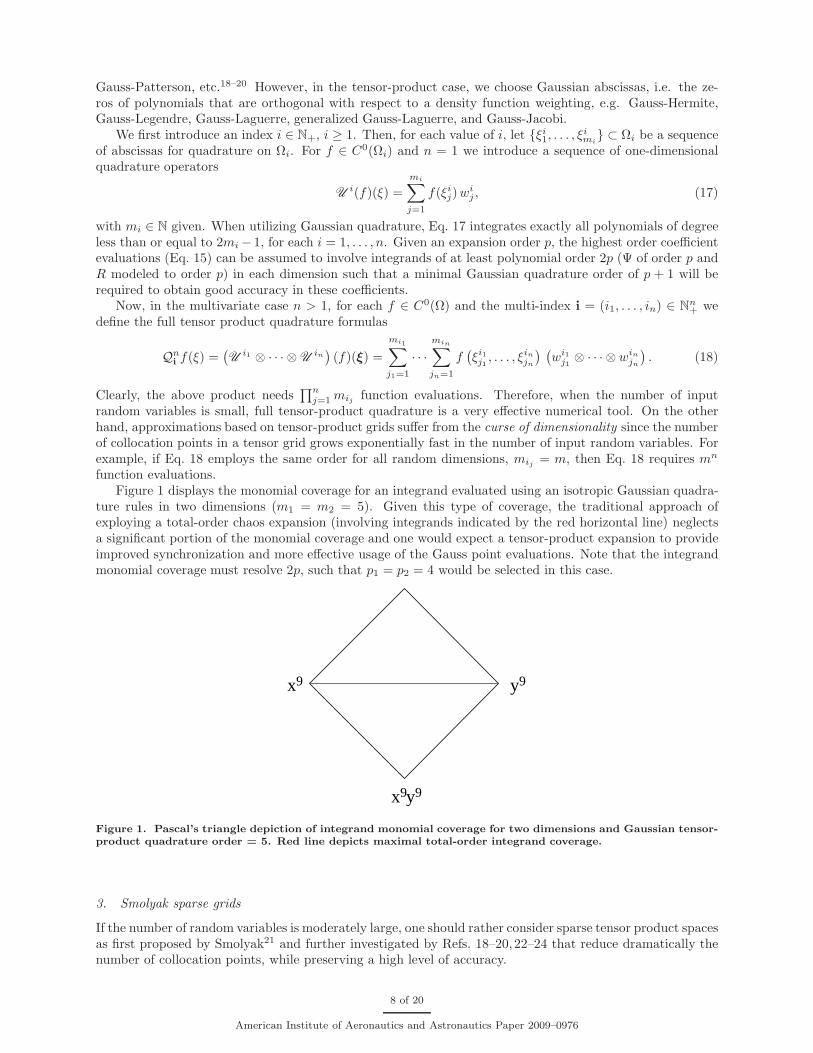
function evaluations.Figure 1 displays the monomial coverage for an integrand evaluated using an isotropic Gaussian quadra-

ture rules in two dimensions (m1 = m2 = 5). Given this type of coverage, the traditional approach ofexploying a total-order chaos expansion (involving integrands indicated by the red horizontal line) neglectsa significant portion of the monomial coverage and one would expect a tensor-product expansion to provideimproved synchronization and more effective usage of the Gauss point evaluations. Note that the integrandmonomial coverage must resolve 2p, such that p1 = p2 = 4 would be selected in this case.

x9y9

y9x9

Figure 1. Pascal’s triangle depiction of integrand monomial coverage for two dimensions and Gaussian tensor-product quadrature order = 5. Red line depicts maximal total-order integrand coverage.

3. Smolyak sparse grids

If the number of random variables is moderately large, one should rather consider sparse tensor product spacesas first proposed by Smolyak21 and further investigated by Refs. 18–20,22–24 that reduce dramatically thenumber of collocation points, while preserving a high level of accuracy.

8 of 20


Here we follow the notation and extend the description in Ref. 18 to describe the Smolyak isotropic

formulas A (w, n), where w is a level that is independent of dimensionc. The Smolyak formulas are justlinear combinations of the product formulas in Eq. 18 with the following key property: only products witha relatively small number of points are used. With U 0 = 0 and for i ≥ 1 define

∆i = Ui − U

i−1. (19)

and we set |i| = i1 + · · · + in. Then the isotropic Smolyak quadrature formula is given by

A (w, n) =∑

|i|≤w+n

(

∆i1 ⊗ · · · ⊗ ∆in)

. (20)

Equivalently, formula Eq. 20 can be written as25

A (w, n) =∑

w+1≤|i|≤w+n

(−1)w+n−|i|(

n− 1

w + n− |i|

)

·(

Ui1 ⊗ · · · ⊗ U

in)

. (21)

Given an index set of levels, growth rules must be defined for the one-dimensional quadrature orders. Inorder to take advantage of nesting and provide similar growth behavior for fully nested and weakly nestedintegration rules, the following nonlinear growth rules are currently employed:

Clenshaw − Curtis : m =

1 w = 0

2w + 1 w ≥ 1(22)

Gaussian : m = 2w+1 − 1 (23)

Examples of isotropic sparse grids, constructed from the fully nested Clenshaw-Curtis abscissas and theweakly-nested Gaussian abscissas are shown in Figure 2, where Ω = [−1, 1]2. There, we consider a two-dimensional parameter space and a maximum level w = 5 (sparse grid A (5, 2)). To see the reduction infunction evaluations with respect to full tensor product grids, we also include a plot of the correspondingClenshaw-Curtis isotropic full tensor grid having the same maximum number of points in each direction,namely 2w + 1 = 33. Whereas an isotropic tensor-product quadrature scales as mn, an isotropic sparse gridscales as mlog n, significantly mitigating the curse of dimensionality.

Figure 2. For a two-dimensional parameter space (n = 2) and maximum level w = 5, we plot the full tensorproduct grid using the Clenshaw-Curtis abscissas (left) and isotropic Smolyak sparse grids A (5, 2), utilizingthe Clenshaw-Curtis abscissas (middle) and the Gaussian abscissas (right).

Figure 3 displays the monomial coverage for an isotropic sparse grid with level w = 4 employing Gaussianintegration rules in two dimensions. Figure 3(a) shows the case of nonlinear growth rules as given in Eq. 23and Figure 3(b) shows an alternative linear growth rule of m = 2w + 1. Given this type of coverage, thetraditional approach of exploying a total-order chaos expansion (maximal resolvable total-order integrand

cOther common formulations use a dimension-dependent level q where q ≥ n. We use w = q − n, where w ≥ 0 for all n.

9 of 20


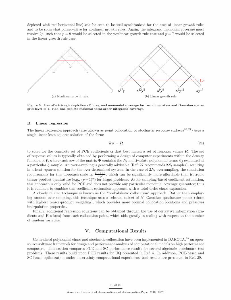
depicted with red horizontal line) can be seen to be well synchronized for the case of linear growth rulesand to be somewhat conservative for nonlinear growth rules. Again, the integrand monomial coverage mustresolve 2p, such that p = 9 would be selected in the nonlinear growth rule case and p = 7 would be selectedin the linear growth rule case.

61yx

x y529

x13y13

x5y29

xy61

19

(a) Nonlinear growth rule.

x13y5 x5y13x9y9 xy17x17y

15

(b) Linear growth rule.

Figure 3. Pascal’s triangle depiction of integrand monomial coverage for two dimensions and Gaussian sparsegrid level = 4. Red line depicts maximal total-order integrand coverage.

B. Linear regression

The linear regression approach (also known as point collocation or stochastic response surfaces26, 27) uses asingle linear least squares solution of the form:

Ψα = R (24)

to solve for the complete set of PCE coefficients α that best match a set of response values R. The setof response values is typically obtained by performing a design of computer experiments within the densityfunction of ξ, where each row of the matrix Ψ contains the Nt multivariate polynomial terms Ψj evaluated ata particular ξ sample. An over-sampling is generally advisable (Ref. 27 recommends 2Nt samples), resultingin a least squares solution for the over-determined system. In the case of 2Nt oversampling, the simulation

requirements for this approach scale as 2(n+p)!n!p! , which can be significantly more affordable than isotropic

tensor-product quadrature (e.g., (p+ 1)n) for larger problems. As for sampling-based coefficient estimation,this approach is only valid for PCE and does not provide any particular monomial coverage guarantee; thusit is common to combine this coefficient estimation approach with a total-order chaos expansion.

A closely related technique is known as the “probabilistic collocation” approach. Rather than employ-ing random over-sampling, this technique uses a selected subset of Nt Gaussian quadrature points (thosewith highest tensor-product weighting), which provides more optimal collocation locations and preservesinterpolation properties.

Finally, additional regression equations can be obtained through the use of derivative information (gra-dients and Hessians) from each collocation point, which aids greatly in scaling with respect to the numberof random variables.

V. Computational Results

Generalized polynomial chaos and stochastic collocation have been implemented in DAKOTA,28 an open-source software framework for design and performance analysis of computational models on high performancecomputers. This section compares PCE and SC performance results for several algebraic benchmark testproblems. These results build upon PCE results for UQ presented in Ref. 5. In addition, PCE-based andSC-based optimization under uncertainty computational experiments and results are presented in Ref. 29.

10 of 20


A. Lognormal ratio

This test problem has a limit state function (i.e., a critical response metric which defines the boundarybetween safe and failed regions of the random variable parameter space) defined by the ratio of two correlated,identically-distributed random variables.

g(x) =x1

x2(25)

The distributions for both x1 and x2 are Lognormal(1, 0.5) with a correlation coefficient between the twovariables of 0.3. A nonlinear variable transformation is applied and Hermite orthogonal polynomials areemployed in the transformed space.

1. Uncertainty quantification with PCE

For the UQ analysis, 24 response levels (.4, .5, .55, .6, .65, .7, .75, .8, .85, .9, 1, 1.05, 1.15, 1.2, 1.25, 1.3, 1.35,1.4, 1.5, 1.55, 1.6, 1.65, 1.7, and 1.75) are mapped into the corresponding cumulative probability levels. Forthis problem, an analytic solution is available and is used for comparison to CDFs generated from samplingon the chaos expansions using 104, 105, or 106 samples.

In Figure 4, CDF residuals are plotted for each of the four PCE coefficient estimation approaches on a log-log graph as a function of increasing simulation evaluations. In all cases, an isotropic total-order expansion isused. For the quadrature approach, the expansion order p is varied from 0 to 10, with the quadrature orderset at p + 1. For the Smolyak sparse grid approach, the level w is varied from 0 to 4, with the expansionorder p set based on the empirically-derived heuristic 2p ≤ m where m is defined from Eq. 23. For thepoint collocation approach, the expansion order is varied from 0 to 10 with the over-sampling ratio set at2. And for the sampling approach, the expansion order is fixed at 10 and the expansion samples are variedbetween 1 and 105 by orders of 10. It is evident that the convergence rates for quadrature, sparse grid, andpoint collocation are super-algebraic/exponential in nature with respect to simulation evaluations, whereasthe convergence rate for sampling is algebraic with the expected slope of − 1

2 (sample estimates converge asthe square root of the number of samples). Increasing the number of samples used to numerically evaluatethe expansion CDFs (104, 105, or 106 samples) demonstrates that the flat regions in the former three plotsare artifacts of the resolution of the sample set, such that these convergence trajectories could be extendedfurther with additional CDF sampling.

100

101

102

103

104

105

10−4

10−3

10−2

10−1

100

101

Simulations

CD

F R

esid

ual

quad m = 1−11, 104 CDF samples



pt colloc ratio = 2, 104 CDF samples



exp samples, p = 10, 104 CDF samples



sparse w = 0−4, 104 CDF samples



Figure 4. Convergence of traditional PCE with each of the coefficient estimation approaches for the lognormalratio test problem. CDF residual is shown versus increasing simulation evaluations on a log-log scale.

In Figure 5, the effects of expansion tailoring are demonstrated through use of tensor-product chaosexpansions that are synchronized with tensor-product quadrature and use of total-order expansions that

11 of 20


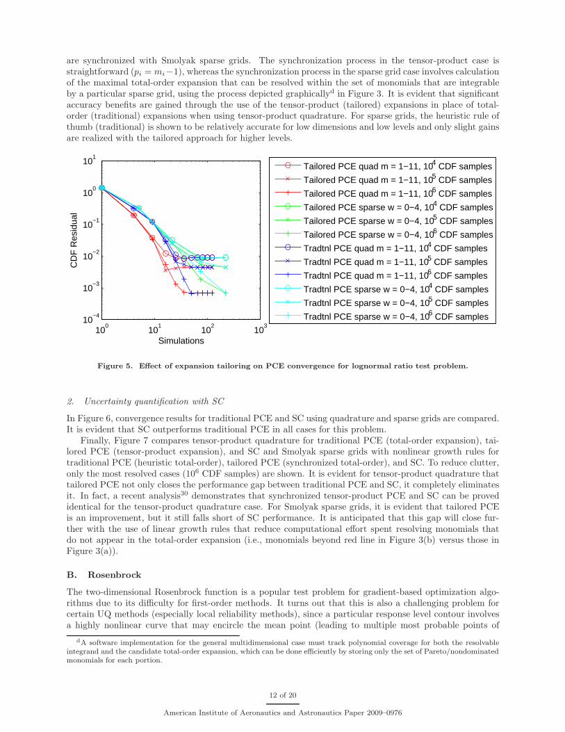
are synchronized with Smolyak sparse grids. The synchronization process in the tensor-product case isstraightforward (pi = mi−1), whereas the synchronization process in the sparse grid case involves calculationof the maximal total-order expansion that can be resolved within the set of monomials that are integrableby a particular sparse grid, using the process depicted graphicallyd in Figure 3. It is evident that significantaccuracy benefits are gained through the use of the tensor-product (tailored) expansions in place of total-order (traditional) expansions when using tensor-product quadrature. For sparse grids, the heuristic rule ofthumb (traditional) is shown to be relatively accurate for low dimensions and low levels and only slight gainsare realized with the tailored approach for higher levels.

100

101

102

103

10−4

10−3

10−2

10−1

100

101

Simulations

CD

F R

esid

ual

Tailored PCE quad m = 1−11, 104 CDF samples



Tailored PCE sparse w = 0−4, 104 CDF samples



Tradtnl PCE quad m = 1−11, 104 CDF samples



Tradtnl PCE sparse w = 0−4, 104 CDF samples



Figure 5. Effect of expansion tailoring on PCE convergence for lognormal ratio test problem.

2. Uncertainty quantification with SC

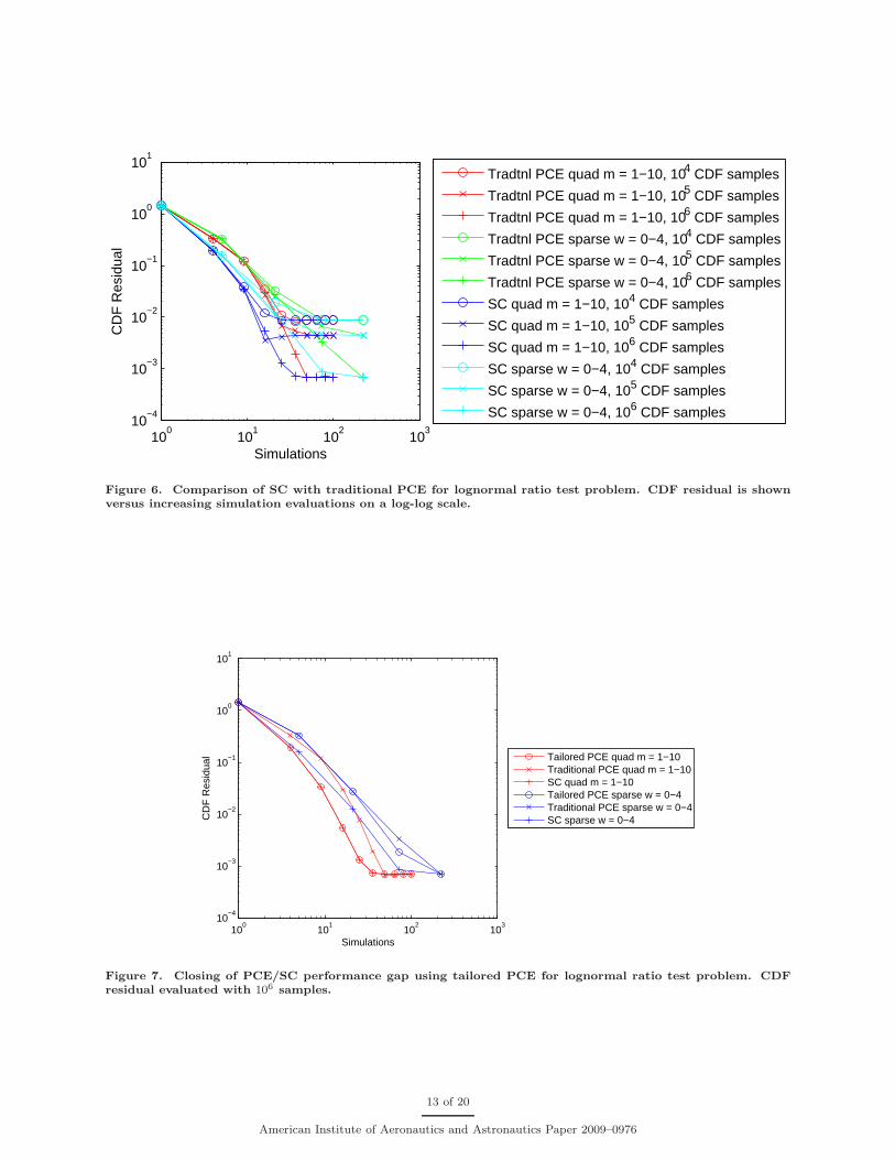
In Figure 6, convergence results for traditional PCE and SC using quadrature and sparse grids are compared.It is evident that SC outperforms traditional PCE in all cases for this problem.

Finally, Figure 7 compares tensor-product quadrature for traditional PCE (total-order expansion), tai-lored PCE (tensor-product expansion), and SC and Smolyak sparse grids with nonlinear growth rules fortraditional PCE (heuristic total-order), tailored PCE (synchronized total-order), and SC. To reduce clutter,only the most resolved cases (106 CDF samples) are shown. It is evident for tensor-product quadrature thattailored PCE not only closes the performance gap between traditional PCE and SC, it completely eliminatesit. In fact, a recent analysis30 demonstrates that synchronized tensor-product PCE and SC can be provedidentical for the tensor-product quadrature case. For Smolyak sparse grids, it is evident that tailored PCEis an improvement, but it still falls short of SC performance. It is anticipated that this gap will close fur-ther with the use of linear growth rules that reduce computational effort spent resolving monomials thatdo not appear in the total-order expansion (i.e., monomials beyond red line in Figure 3(b) versus those inFigure 3(a)).

B. Rosenbrock

The two-dimensional Rosenbrock function is a popular test problem for gradient-based optimization algo-rithms due to its difficulty for first-order methods. It turns out that this is also a challenging problem forcertain UQ methods (especially local reliability methods), since a particular response level contour involvesa highly nonlinear curve that may encircle the mean point (leading to multiple most probable points of

dA software implementation for the general multidimensional case must track polynomial coverage for both the resolvableintegrand and the candidate total-order expansion, which can be done efficiently by storing only the set of Pareto/nondominatedmonomials for each portion.

12 of 20


100

101

102

103

10−4

10−3

10−2

10−1

100

101

Simulations

CD

F R

esid

ual







SC quad m = 1−10, 104 CDF samples



SC sparse w = 0−4, 104 CDF samples



Figure 6. Comparison of SC with traditional PCE for lognormal ratio test problem. CDF residual is shownversus increasing simulation evaluations on a log-log scale.

100

101

102

103

10−4

10−3

10−2

10−1

100

101

Simulations

CD

F R

esid

ual

Tailored PCE quad m = 1−10Traditional PCE quad m = 1−10SC quad m = 1−10Tailored PCE sparse w = 0−4Traditional PCE sparse w = 0−4SC sparse w = 0−4

Figure 7. Closing of PCE/SC performance gap using tailored PCE for lognormal ratio test problem. CDFresidual evaluated with 106 samples.

13 of 20


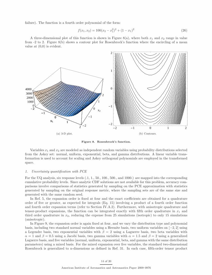
failure). The function is a fourth order polynomial of the form:

f(x1, x2) = 100(x2 − x21)

2 + (1 − x1)2 (26)

A three-dimensional plot of this function is shown in Figure 8(a), where both x1 and x2 range in valuefrom -2 to 2. Figure 8(b) shows a contour plot for Rosenbrock’s function where the encircling of a meanvalue at (0,0) is evident.

-2-1

0

1

2

x1

-2

-1

0

1

2

x2

01000200030004000

-2-1

0

1

2

x1

(a) 3-D plot.

-2 -1 0 1 2-2

-1

0

1

2

(b) Contours.

Figure 8. Rosenbrock’s function.

Variables x1 and x2 are modeled as independent random variables using probability distributions selectedfrom the Askey set: normal, uniform, exponential, beta, and gamma distributions. A linear variable trans-formation is used to account for scaling and Askey orthogonal polynomials are employed in the transformedspace.

1. Uncertainty quantification with PCE

For the UQ analysis, six response levels (.1, 1., 50., 100., 500., and 1000.) are mapped into the correspondingcumulative probability levels. Since analytic CDF solutions are not available for this problem, accuracy com-parisons involve comparisons of statistics generated by sampling on the PCE approximation with statisticsgenerated by sampling on the original response metric, where the sampling sets are of the same size andgenerated with the same random seed.

In Ref. 5, the expansion order is fixed at four and the exact coefficients are obtained for a quadratureorder of five or greater, as expected for integrals (Eq. 15) involving a product of a fourth order functionand fourth order expansion terms (refer to Section IV.A.2). Furthermore, with anisotropic quadrature andtensor-product expansions, the function can be integrated exactly with fifth order quadrature in x1 andthird order quadrature in x2, reducing the expense from 25 simulations (isotropic) to only 15 simulations(anisotropic).

In Figure 9, the expansion order is again fixed at four, and we vary the distribution type and polynomialbasis, including two standard normal variables using a Hermite basis, two uniform variables on [−2, 2] usinga Legendre basis, two exponential variables with β = 2 using a Laguerre basis, two beta variables withα = 1 and β = 0.5 using a Jacobi basis, two gamma variables with α = 1.5 and β = 2 using a generalizedLaguerre basis, and five variables (normal, uniform, exponential, beta, and gamma with the same distributionparameters) using a mixed basis. For the mixed expansion over five variables, the standard two-dimensionalRosenbrock is generalized to n-dimensions as defined in Ref. 31. In each case, fifth-order tensor product

14 of 20


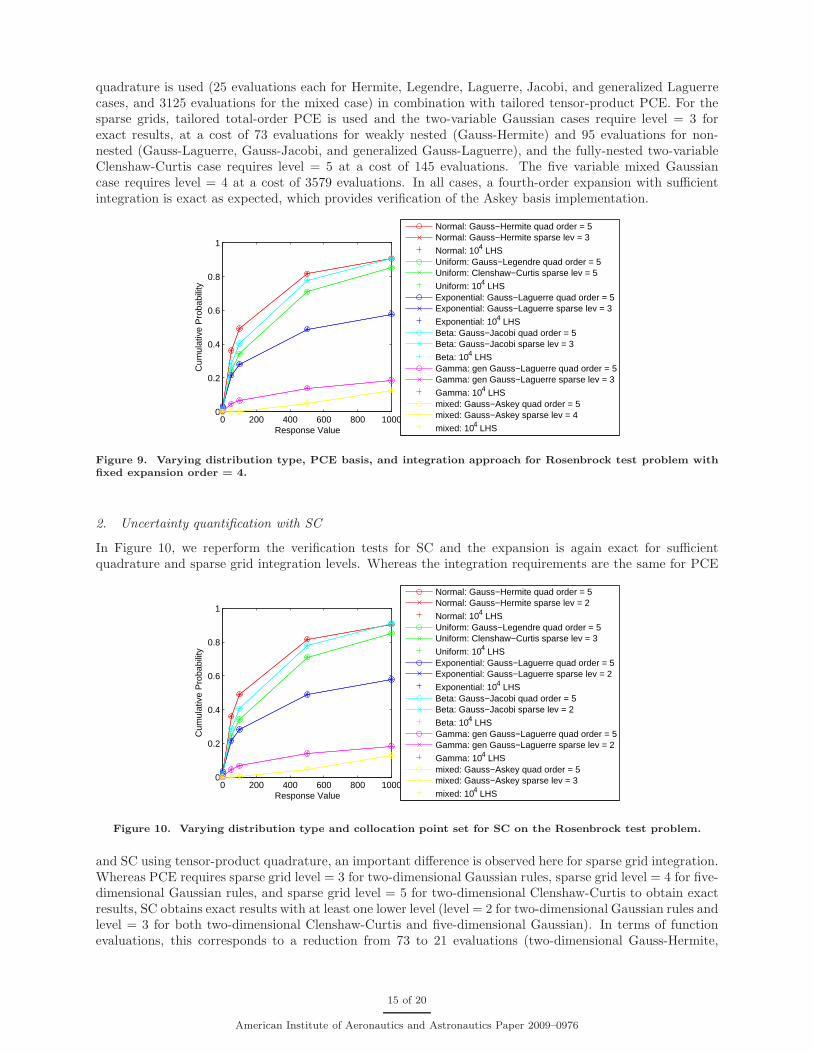
quadrature is used (25 evaluations each for Hermite, Legendre, Laguerre, Jacobi, and generalized Laguerrecases, and 3125 evaluations for the mixed case) in combination with tailored tensor-product PCE. For thesparse grids, tailored total-order PCE is used and the two-variable Gaussian cases require level = 3 forexact results, at a cost of 73 evaluations for weakly nested (Gauss-Hermite) and 95 evaluations for non-nested (Gauss-Laguerre, Gauss-Jacobi, and generalized Gauss-Laguerre), and the fully-nested two-variableClenshaw-Curtis case requires level = 5 at a cost of 145 evaluations. The five variable mixed Gaussiancase requires level = 4 at a cost of 3579 evaluations. In all cases, a fourth-order expansion with sufficientintegration is exact as expected, which provides verification of the Askey basis implementation.

0 200 400 600 800 10000

0.2

0.4

0.6

0.8

1

Response Value

Cum

ulat

ive

Pro

babi

lity

Normal: Gauss−Hermite quad order = 5Normal: Gauss−Hermite sparse lev = 3

Normal: 104 LHSUniform: Gauss−Legendre quad order = 5Uniform: Clenshaw−Curtis sparse lev = 5

Uniform: 104 LHSExponential: Gauss−Laguerre quad order = 5Exponential: Gauss−Laguerre sparse lev = 3

Exponential: 104 LHSBeta: Gauss−Jacobi quad order = 5Beta: Gauss−Jacobi sparse lev = 3

Beta: 104 LHSGamma: gen Gauss−Laguerre quad order = 5Gamma: gen Gauss−Laguerre sparse lev = 3

Gamma: 104 LHSmixed: Gauss−Askey quad order = 5mixed: Gauss−Askey sparse lev = 4

mixed: 104 LHS

Figure 9. Varying distribution type, PCE basis, and integration approach for Rosenbrock test problem withfixed expansion order = 4.

2. Uncertainty quantification with SC

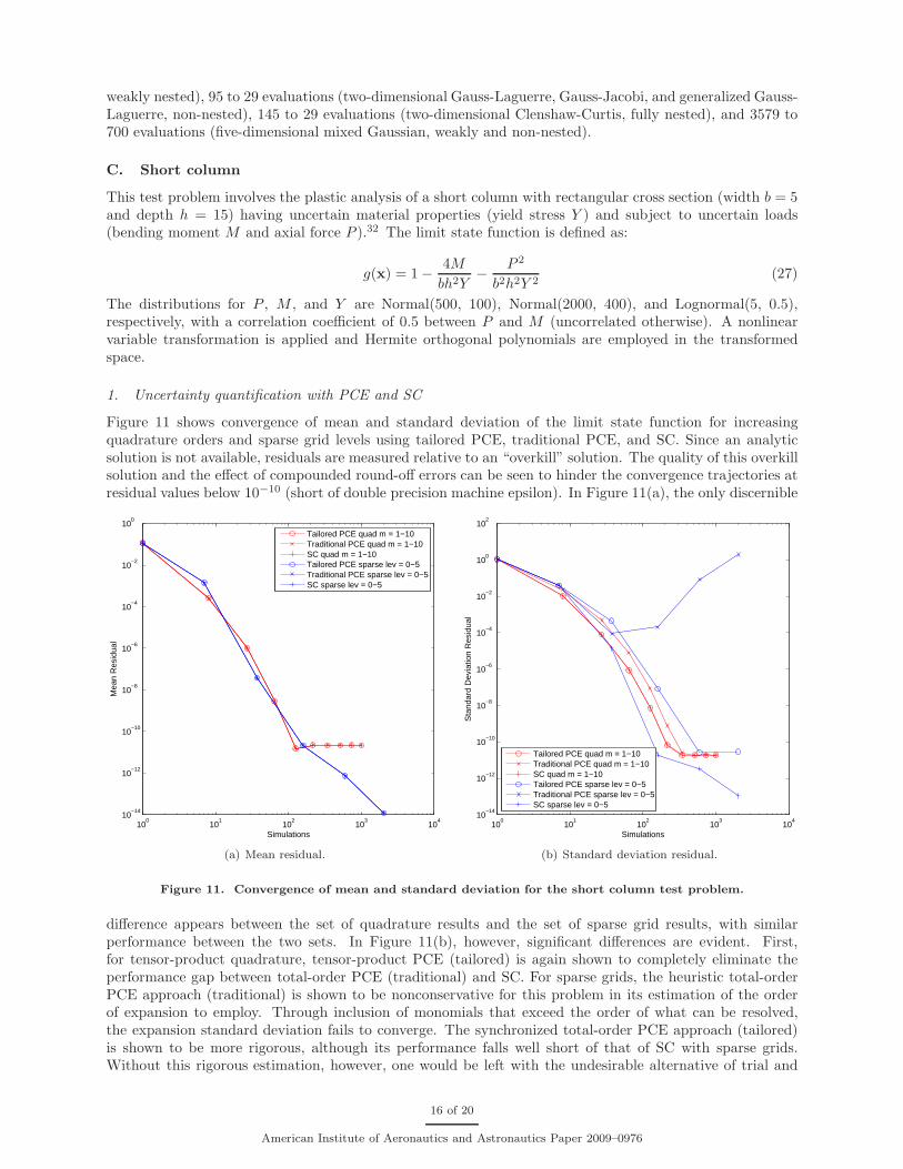
In Figure 10, we reperform the verification tests for SC and the expansion is again exact for sufficientquadrature and sparse grid integration levels. Whereas the integration requirements are the same for PCE

0 200 400 600 800 10000

0.2

0.4

0.6

0.8

1

Response Value

Cum

ulat

ive

Pro

babi

lity

Normal: Gauss−Hermite quad order = 5Normal: Gauss−Hermite sparse lev = 2

Normal: 104 LHSUniform: Gauss−Legendre quad order = 5Uniform: Clenshaw−Curtis sparse lev = 3

Uniform: 104 LHSExponential: Gauss−Laguerre quad order = 5Exponential: Gauss−Laguerre sparse lev = 2

Exponential: 104 LHSBeta: Gauss−Jacobi quad order = 5Beta: Gauss−Jacobi sparse lev = 2

Beta: 104 LHSGamma: gen Gauss−Laguerre quad order = 5Gamma: gen Gauss−Laguerre sparse lev = 2

Gamma: 104 LHSmixed: Gauss−Askey quad order = 5mixed: Gauss−Askey sparse lev = 3

mixed: 104 LHS

Figure 10. Varying distribution type and collocation point set for SC on the Rosenbrock test problem.

and SC using tensor-product quadrature, an important difference is observed here for sparse grid integration.Whereas PCE requires sparse grid level = 3 for two-dimensional Gaussian rules, sparse grid level = 4 for five-dimensional Gaussian rules, and sparse grid level = 5 for two-dimensional Clenshaw-Curtis to obtain exactresults, SC obtains exact results with at least one lower level (level = 2 for two-dimensional Gaussian rules andlevel = 3 for both two-dimensional Clenshaw-Curtis and five-dimensional Gaussian). In terms of functionevaluations, this corresponds to a reduction from 73 to 21 evaluations (two-dimensional Gauss-Hermite,

15 of 20


weakly nested), 95 to 29 evaluations (two-dimensional Gauss-Laguerre, Gauss-Jacobi, and generalized Gauss-Laguerre, non-nested), 145 to 29 evaluations (two-dimensional Clenshaw-Curtis, fully nested), and 3579 to700 evaluations (five-dimensional mixed Gaussian, weakly and non-nested).

C. Short column

This test problem involves the plastic analysis of a short column with rectangular cross section (width b = 5and depth h = 15) having uncertain material properties (yield stress Y ) and subject to uncertain loads(bending moment M and axial force P ).32 The limit state function is defined as:

g(x) = 1 −4M

bh2Y−

P 2

b2h2Y 2(27)

The distributions for P , M , and Y are Normal(500, 100), Normal(2000, 400), and Lognormal(5, 0.5),respectively, with a correlation coefficient of 0.5 between P and M (uncorrelated otherwise). A nonlinearvariable transformation is applied and Hermite orthogonal polynomials are employed in the transformedspace.

1. Uncertainty quantification with PCE and SC

Figure 11 shows convergence of mean and standard deviation of the limit state function for increasingquadrature orders and sparse grid levels using tailored PCE, traditional PCE, and SC. Since an analyticsolution is not available, residuals are measured relative to an “overkill” solution. The quality of this overkillsolution and the effect of compounded round-off errors can be seen to hinder the convergence trajectories atresidual values below 10−10 (short of double precision machine epsilon). In Figure 11(a), the only discernible

100

101

102

103

104

10−14

10−12

10−10

10−8

10−6

10−4

10−2

100

Simulations

Mea

n R

esid

ual

Tailored PCE quad m = 1−10Traditional PCE quad m = 1−10SC quad m = 1−10Tailored PCE sparse lev = 0−5Traditional PCE sparse lev = 0−5SC sparse lev = 0−5

(a) Mean residual.

100

101

102

103

104

10−14

10−12

10−10

10−8

10−6

10−4

10−2

100

102

Simulations

Sta

ndar

d D

evia

tion

Res

idua

l


(b) Standard deviation residual.

Figure 11. Convergence of mean and standard deviation for the short column test problem.

difference appears between the set of quadrature results and the set of sparse grid results, with similarperformance between the two sets. In Figure 11(b), however, significant differences are evident. First,for tensor-product quadrature, tensor-product PCE (tailored) is again shown to completely eliminate theperformance gap between total-order PCE (traditional) and SC. For sparse grids, the heuristic total-orderPCE approach (traditional) is shown to be nonconservative for this problem in its estimation of the orderof expansion to employ. Through inclusion of monomials that exceed the order of what can be resolved,the expansion standard deviation fails to converge. The synchronized total-order PCE approach (tailored)is shown to be more rigorous, although its performance falls well short of that of SC with sparse grids.Without this rigorous estimation, however, one would be left with the undesirable alternative of trial and

16 of 20


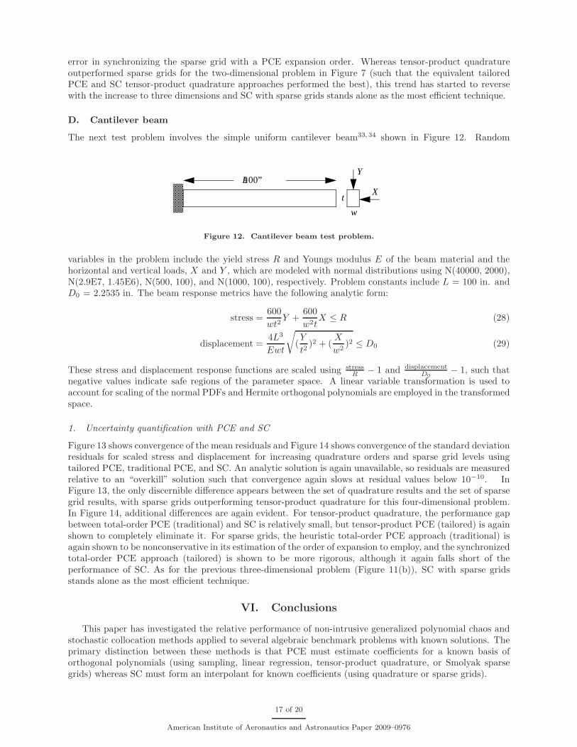
error in synchronizing the sparse grid with a PCE expansion order. Whereas tensor-product quadratureoutperformed sparse grids for the two-dimensional problem in Figure 7 (such that the equivalent tailoredPCE and SC tensor-product quadrature approaches performed the best), this trend has started to reversewith the increase to three dimensions and SC with sparse grids stands alone as the most efficient technique.

D. Cantilever beam

The next test problem involves the simple uniform cantilever beam33, 34 shown in Figure 12. Random

L = 100”

w

tX

Y

Figure 12. Cantilever beam test problem.

variables in the problem include the yield stress R and Youngs modulus E of the beam material and thehorizontal and vertical loads, X and Y , which are modeled with normal distributions using N(40000, 2000),N(2.9E7, 1.45E6), N(500, 100), and N(1000, 100), respectively. Problem constants include L = 100 in. andD0 = 2.2535 in. The beam response metrics have the following analytic form:

stress =600

wt2Y +

600

w2tX ≤ R (28)

displacement =4L3

Ewt

√

(Y

t2)2 + (

X

w2)2 ≤ D0 (29)

These stress and displacement response functions are scaled using stressR

− 1 and displacementD0

− 1, such thatnegative values indicate safe regions of the parameter space. A linear variable transformation is used toaccount for scaling of the normal PDFs and Hermite orthogonal polynomials are employed in the transformedspace.

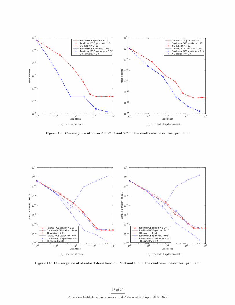
1. Uncertainty quantification with PCE and SC

Figure 13 shows convergence of the mean residuals and Figure 14 shows convergence of the standard deviationresiduals for scaled stress and displacement for increasing quadrature orders and sparse grid levels usingtailored PCE, traditional PCE, and SC. An analytic solution is again unavailable, so residuals are measuredrelative to an “overkill” solution such that convergence again slows at residual values below 10−10. InFigure 13, the only discernible difference appears between the set of quadrature results and the set of sparsegrid results, with sparse grids outperforming tensor-product quadrature for this four-dimensional problem.In Figure 14, additional differences are again evident. For tensor-product quadrature, the performance gapbetween total-order PCE (traditional) and SC is relatively small, but tensor-product PCE (tailored) is againshown to completely eliminate it. For sparse grids, the heuristic total-order PCE approach (traditional) isagain shown to be nonconservative in its estimation of the order of expansion to employ, and the synchronizedtotal-order PCE approach (tailored) is shown to be more rigorous, although it again falls short of theperformance of SC. As for the previous three-dimensional problem (Figure 11(b)), SC with sparse gridsstands alone as the most efficient technique.

VI. Conclusions

This paper has investigated the relative performance of non-intrusive generalized polynomial chaos andstochastic collocation methods applied to several algebraic benchmark problems with known solutions. Theprimary distinction between these methods is that PCE must estimate coefficients for a known basis oforthogonal polynomials (using sampling, linear regression, tensor-product quadrature, or Smolyak sparsegrids) whereas SC must form an interpolant for known coefficients (using quadrature or sparse grids).

17 of 20


100

101

102

103

104

10−14

10−12

10−10

10−8

10−6

10−4

10−2

Simulations

Mea

n R

esid

ual


(a) Scaled stress.

100

101

102

103

104

10−14

10−12

10−10

10−8

10−6

10−4

10−2

100

SimulationsM

ean

Res

idua

l


(b) Scaled displacement.

Figure 13. Convergence of mean for PCE and SC in the cantilever beam test problem.

100

101

102

103

104

10−14

10−12

10−10

10−8

10−6

10−4

10−2

100

102

Simulations

Sta

ndar

d D

evia

tion

Res

idua

l


(a) Scaled stress.

100

101

102

103

104

10−14

10−12

10−10

10−8

10−6

10−4

10−2

100

102

Simulations

Sta

ndar

d D

evia

tion

Res

idua

l


(b) Scaled displacement.

Figure 14. Convergence of standard deviation for PCE and SC in the cantilever beam test problem.

18 of 20


Performance between these methods is shown to be very similar and both demonstrate impressive effi-ciency relative to Monte Carlo sampling methods and impressive accuracy relative to reliability methods.When a difference is observed between traditional PCE and SC, SC has been the consistent winner, typi-cally manifesting in the reduction of the required integration by one order or level. This difference can belargely attributed to expansion/integration synchronization issues with PCE, motivating the approaches fortailoring of chaos expansions that are explored in this paper.

For the case of tensor-product quadrature, tailored tensor-product PCE is shown to perform identicallyto SC such that the performance gap is completely eliminated. Both methods consistently outperformtraditional PCE. However, tensor-product quadrature approaches only outperform sparse grid approachesfor the lowest dimensional problems.

For problems with greater than two dimensions, sparse grid approaches are shown to outperform tensor-product quadrature approaches. For sparse grids, selection of a synchronized PCE formulation is nontrivialand the tailored total-order PCE approach, which computes the maximal total-order expansion that can beresolved by a particular sparse grid, is shown to be more rigorous and reliable than heuristics and eliminatesinefficiency due to trial and error. A significant performance gap relative to SC with sparse grids still remainsfor the case of nonlinear sparse grid growth rules, but replacement of these rules with linear ones (at leastfor Gaussian quadratures that are at most weakly nested) will reduce the set of resolvable monomials thatdo not appear in the total-order expansion. This is expected to close the performance gap to some degree.However, it is not expected that any nonintrusive PCE approach will outperform SC when using the same setof collocation points. Rather, usage of PCE remains motivated by other practical considerations, in particularits greater flexibility in collocation point selection (i.e., Genz cubature grids as well as unstructured/randompoint sets that can support greater simulation fault tolerance).

Future work will investigate these linear sparse grid growth rules as well as sparse grids that supportanisotropy in level and numerically-generated polynomials that preserve exponential convergence rates forarbitrary input PDFs.

Acknowledgments

The authors thank Paul Constantine and Gianluca Iaccarino of Stanford University for sharing theiranalysis on the equivalence of tensor-product PCE and SC, which largely motivated the exploration of PCEtailoring in this work. The authors also thank Clayton Webster for his development of concepts and analysisfor anisotropic sparse grids. Finally, the authors thank the DOE Accelerated Strategic Computing (ASC)program for support of this collaborative work between Sandia National Laboratories and Virginia Tech.

References

1Xiu, D. and Karniadakis, G. M., “The Wiener-Askey Polynomial Chaos for Stochastic Differential Equations,” SIAM J.Sci. Comput., Vol. 24, No. 2, 2002, pp. 619–644.

2Askey, R. and Wilson, J., “Some Basic Hypergeometric Polynomials that Generalize Jacobi Polynomials,” Mem. Amer.Math. Soc. 319 , AMS, Providence, RI, 1985.

3Wiener, N., “The Homogoeneous Chaos,” Amer. J. Math., Vol. 60, 1938, pp. 897–936.4Abramowitz, M. and Stegun, I. A., Handbook of Mathematical Functions with Formulas, Graphs, and Mathematical

Tables, Dover, New York, 1965.5Eldred, M. S., Webster, C. G., and Constantine, P., “Evaluation of Non-Intrusive Approaches for Wiener-Askey Gen-

eralized Polynomial Chaos,” Proceedings of the 10th AIAA Nondeterministic Approaches Conference, No. AIAA-2008-1892,Schaumburg, IL, April 7–10 2008.

6Der Kiureghian, A. and Liu, P. L., “Structural Reliability Under Incomplete Probability Information,” J. Eng. Mech.,ASCE , Vol. 112, No. 1, 1986, pp. 85–104.

7Golub, G. H. and Welsch, J. H., “Caclulation of Gauss Quadrature Rules,” Mathematics of Computation, Vol. 23, No.106, 1969, pp. 221–230.

8Witteveen, J. A. S. and Bijl, H., “Modeling Arbitrary Uncertainties Using Gram-Schmidt Polynomial Chaos,” Proceedingsof the 44th AIAA Aerospace Sciences Meeting and Exhibit, No. AIAA-2006-0896, Reno, NV, January 9–12 2006.

9Eldred, M. S., “Recent Advances in Non-Intrusive Polynomial Chaos and Stochastic Collocation Methods for UncertaintyAnalysis and Design,” to appear in Proceedings of the 11th AIAA Nondeterministic Approaches Conference, No. AIAA-2009-2274, Palm Springs, CA, May 4–7 2009.

10Ghanem, R. G., private communication.11Eldred, M. S., Agarwal, H., Perez, V. M., Wojtkiewicz, Jr., S. F., and Renaud, J. E., “Investigation of Reliability Method

Formulations in DAKOTA/UQ,” Structure & Infrastructure Engineering: Maintenance, Management, Life-Cycle Design &Performance, Vol. 3, No. 3, 2007, pp. 199–213.

19 of 20


12Eldred, M. S. and Bichon, B. J., “Second-Order Reliability Formulations in DAKOTA/UQ,” Proceedings of the 47thAIAA/ASME/ASCE/AHS/ASC Structures, Structural Dynamics and Materials Conference, No. AIAA-2006-1828, New-port, RI, May 1–4 2006.

13Rosenblatt, M., “Remarks on a Multivariate Transformation,” Ann. Math. Stat., Vol. 23, No. 3, 1952, pp. 470–472.14Box, G. E. P. and Cox, D. R., “An Analysis of Transformations,” J. Royal Stat. Soc., Vol. 26, 1964, pp. 211–252.15Rackwitz, R. and Fiessler, B., “Structural Reliability under Combined Random Load Sequences,” Comput. Struct., Vol. 9,

1978, pp. 489–494.16Chen, X. and Lind, N. C., “Fast Probability Integration by Three-Parameter Normal Tail Approximation,” Struct. Saf.,

Vol. 1, 1983, pp. 269–276.17Wu, Y.-T. and Wirsching, P. H., “A New Algorithm for Structural Reliability Estimation,” J. Eng. Mech., ASCE ,

Vol. 113, 1987, pp. 1319–1336.18Nobile, F., Tempone, R., and Webster, C. G., “A Sparse Grid Stochastic Collocation Method for Partial Differential

Equations with Random Input Data,” SIAM J. on Num. Anal., 2008, To appear.19Nobile, F., Tempone, R., and Webster, C. G., “An Anisotropic Sparse Grid Stochastic Collocation Method for Partial

Differential Equations with Random Input Data,” SIAM J. on Num. Anal., 2008, To appear.20Gerstner, T. and Griebel, M., “Numerical integration using sparse grids,” Numer. Algorithms, Vol. 18, No. 3-4, 1998,

pp. 209–232.21Smolyak, S., “Quadrature and interpolation formulas for tensor products of certain classes of functions,” Dokl. Akad.

Nauk SSSR, Vol. 4, 1963, pp. 240–243.22Barthelmann, V., Novak, E., and Ritter, K., “High dimensional polynomial interpolation on sparse grids,” Adv. Comput.

Math., Vol. 12, No. 4, 2000, pp. 273–288, Multivariate polynomial interpolation.23Frauenfelder, P., Schwab, C., and Todor, R. A., “Finite elements for elliptic problems with stochastic coefficients,”

Comput. Methods Appl. Mech. Engrg., Vol. 194, No. 2-5, 2005, pp. 205–228.24Xiu, D. and Hesthaven, J., “High-order collocation methods for differential equations with random inputs,” SIAM J. Sci.

Comput., Vol. 27, No. 3, 2005, pp. 1118–1139 (electronic).25Wasilkowski, G. W. and Wozniakowski, H., “Explicit Cost Bounds of Algorithms for Multivariate Tensor Product Prob-

lems,” Journal of Complexity , Vol. 11, 1995, pp. 1–56.26Walters, R. W., “Towards Stochastic Fluid Mechanics via Polynomial Chaos,” Proceedings of the 41st AIAA Aerospace

Sciences Meeting and Exhibit , No. AIAA-2003-0413, Reno, NV, January 6–9, 2003.27Hosder, S., Walters, R. W., and Balch, M., “Efficient Sampling for Non-Intrusive Polynomial Chaos Applications with

Multiple Uncertain Input Variables,” Proceedings of the 48th AIAA/ASME/ASCE/AHS/ASC Structures, Structural Dynamics,and Materials Conference, No. AIAA-2007-1939, Honolulu, HI, April 23–26, 2007.

28Eldred, M. S., Adams, B. M., Haskell, K., Bohnhoff, W. J., Eddy, J. P., Gay, D. M., Hart, W. E., Hough, P. D.,Kolda, T. G., Swiler, L. P., and Watson, J.-P., “DAKOTA, A Multilevel Parallel Object-Oriented Framework for DesignOptimization, Parameter Estimation, Uncertainty Quantification, and Sensitivity Analysis: Version 4.2 Users Manual,” Tech.Rep. SAND2006-6337, Sandia National Laboratories, Albuquerque, NM, 2008.

29Eldred, M. S., Webster, C. G., and Constantine, P., “Design Under Uncertainty Employing Stochastic Expansion Meth-ods,” Proceedings of the 12th AIAA/ISSMO Multidisciplinary Analysis and Optimization Conference, No. AIAA-2008-6001,Victoria, British Columbia, September 10–12, 2008.

30Constantine, P. and Iaccarino, G., “Comparing spectral Galerkin and spectral collocation methods for parameterizedmatrix equations.” Tech. Rep. UQ-08-02, Stanford University, Stanford, CA, 2008.

31Schittkowski, K., More Test Examples for Nonlinear Programming, Lecture Notes in Economics and MathematicalSystems, Vol. 282 , Springer-Verlag, Berlin, 1987.

32Kuschel, N. and Rackwitz, R., “Two Basic Problems in Reliability-Based Structural Optimization,” Math. Method Oper.Res., Vol. 46, 1997, pp. 309–333.

33Sues, R., Aminpour, M., and Shin, Y., “Reliability-Based Multidisciplinary Optimization for Aerospace Systems,” Pro-ceedings of the 42rd AIAA/ASME/ASCE/AHS/ASC Structures, Structural Dynamics, and Materials Conference, No. AIAA-2001-1521, Seattle, WA, April 16–19, 2001.

34Wu, Y.-T., Shin, Y., Sues, R., and Cesare, M., “Safety-Factor Based Approach for Probability-Based Design Optimiza-tion,” Proceedings of the 42rd AIAA/ASME/ASCE/AHS/ASC Structures, Structural Dynamics, and Materials Conference,No. AIAA-2001-1522, Seattle, WA, April 16–19, 2001.

20 of 20


comparison of non-intrusive polynomial chaos and stochastic

Documents