COMPARISON OF LIMIT STATES DESIGN WITH WORKING STRESS DESIGN

FOR SHALLOW FOUNDATIONS

by

GEORGIA J. LYSAY

B.Sc. i n C i v i l Engineering, U n i v e r s i t y of Saskatchewan, 1997

A THESIS SUBMITTED IN PARTIAL FULFILMENT OF THE REQUIREMENTS FOR THE DEGREE OF

MASTER OF APPLIED SCIENCE

i n

THE FACULTY OF GRADUATE STUDIES

Department of C i v i l Engineering

We accept t h i s t h e s i s as conforming to the required standard

THE UNIVERSITY OF BRITISH COLUMBIA

August 1999

© Georgia J. Lysay, 1999

U B C Special Collections - Thesis Authorisation Form Page 1 of 1

In p r e s e n t i n g t h i s t h e s i s i n p a r t i a l f u l f i l m e n t of the requirements f o r an advanced degree at the U n i v e r s i t y of B r i t i s h Columbia, I agree t h a t the L i b r a r y s h a l l make i t f r e e l y a v a i l a b l e f o r reference and study. I f u r t h e r agree that permission f o r extensive copying of t h i s t h e s i s f o r s c h o l a r l y purposes may be granted by the head of my department or by h i s or her r e p r e s e n t a t i v e s . I t i s understood t h a t copying or p u b l i c a t i o n of t h i s t h e s i s f o r f i n a n c i a l gain s h a l l not be allowed without my w r i t t e n permission.

Department of '/

The U n i v e r s i t y of B r i t i s h Columbia Vancouver, Canada

http://www.library.ubc.ca/spcoll/thesauth.html 8/6/99

Abstract

Bridge foundations have traditionally been designed using working stress methods, but the new Canadian Highway Bridge Design Code (draft CHBDC) now specifies a limit states design procedure for these structures. The main objective of this study was to compare working stress design (WSD) with limit states design (LSD) methods particular to bridge abutments. The two design methods have been investigated and compared to a numerical model (developed using the program FLAC) . The results of these analyses were compared for reliability and safety.

L S D was applied to an existing bridge abutment (the No. 5 Road Bridge in Richmond, British Columbia) which was initially designed using WSD. The two different designs were compared on the basis of factors of safety with the outcome indicating that the structure having been designed using WSD may be too reliable and overly safe.

A F L A C model of the No. 5 Road overpass abutment was developed and incrementally loaded to failure in order to determine the capacity distribution of the structure. The resulting normal distribution of capacity was used in a reliability analysis with two different models for loading. This analysis yielded a relationship between mean live load and reliability index for this particular structure. The results indicated that the reliability index at the design live load was higher than the value of 3.5 that was used to calibrate the CHBDC LSD partial factors.

The expected displacement during the regional design earthquake was predicted using a F L A C model. The model was run a number of times with various earthquakes and combinations of soil properties. The results of the F L A C runs were combined with joint probabilities of occurrences of soil parameters (derived from a survey) to obtain the expected displacements. The results showed relatively small expected values of displacement which also indicated that the original abutment design may be overly safe in terms of the draft CHBDC. .

A sensitivity analysis involving soil parameters was also considered. The soil properties were varied within the F L A C model to determine the resulting variation in displacements, and to ascertain which variables most affect the outcome of the analysis. Friction angle was found to be the critical soil property, as it had more of an effect on displacements than did (Ni)60 or unit weight.

ii

Table of Contents Page

Abstract i i Table of Contents i i i List of Tables vi List of Figures vii Acknowledgments ix

1. Introduction 1 1.1 Background 1 1.2 Objective 2 1.3 Scope 2

2. Description and Background to Analysis Programs 3 2.1 Introduction 3 2.2 F L A C 3

2.2.1 Finite Difference Method 4 2.2.2 Explicit Time-Marching Scheme 4 2.2.3 Lagrangian Analysis 6 2.2.4 Plasticity Analysis 6

2.3 S H A K E 7 2.3.1 Description of the Program 7 2.3.2 Program Assumptions 7 2.3.3 Implementation of the Program 9

2.4 Reliability Analysis 9 2.4.1 The F O R M method and R E L A N analysis 10

2.5 Summary 12

3. Design Methods and Codes 13 3.1 Introduction 13 3.2 Working Stress Design 14 3.3 Limit States Design 15

3.3.1 Uncertainty in Geotechnical Engineering 16 3.3.2 Compatibility and Economy 16 3.3.3 Ultimate Limit States and Serviceability Limit States 17 3.3.4 Factored Strength 18 3.3.5 Factored Resistance 19 3.3.6 Advantages of Limit States Design 20

3.4 Canadian Bridge Codes 21 3.4.1 Design of Highway Bridges - CS A Standard

CAN3-S6-M78 21 Bearing Capacity 21 Abutments 22

3.4.2 Design of Highway Bridges - CAN/CSA-S6-88 22

iii

Bearing Capacity 23 Abutments 23

3.4.3 Canadian Highway Bridge Design Code - Draft 1998 24 Bearing Capacity 24

3.5 Seismic Design 24 3.5.1 Earthquake Forces -CHBDC Draft 1998 25 3.5.2 ATC-6 Seismic Design Guidelines for Highway

Bridges(1983) 25 3.5.3 Standard Specifications for Highway Bridges

(AASHTO 1989) 25 3.5.4 ATC-32 Improved Seismic Design Criteria for

California Bridges: Provisional Recommendations (1996) 25 3.6 Summary 26

4. F L A C model of Centrifuge Experiment 27 4.1 Introduction 27 4.2 Centrifuge Theory 27 4.3 The Experiment 28 4.4 F L A C Model 30 4.5 Comparison of Centrifuge Experiment and F L A C Model 31

5. No. 5 Road Overpass Abutment - WSD and LSD 34 5.1 Introduction and Background 34 5.2 Working Stress Design 35

5.2.1 Case 1 36 5.2.2 Case 2 36 5.2.3 Case 3 36 5.2.4 Case 4 36 5.2.5 Factors of Safety for WSD 36

5.3 Limit States Design 37 5.3.1 Loads 38 5.3.2 Bearing Capacity 39 5.3.3 Sliding Resistance 41

5.4 Comparison of WSD and LSD Results 44

6. Determination of Reliability Index for No. 5 Road Bridge Abutment 46 6.1 Introduction 46 6.2 Capacity Determined by F L A C 47 6.3 Demand 51 6.4 Reliability Index, B 52 6.5 Alternative Model for Live Load 55 6.6 Summary 56

7. Dynamic Analysis of No. 5 Road Overpass Abutment 57

iv

7.1 S H A K E Analysis 57 7.1.1 Soil Column 57 7.1.2 Input Earthquakes 61 7.1.3 Resulting Accelerations and Amplifications 63

7.2 Comparison with F L A C Column 67 7.3 Questionnaire 68 7.4 F L A C Model for Dynamic Analysis 68 7.5 Expected Value of Displacement 69 7.6 Sensitivity Analysis in F L A C 73

7.6.1 Friction Angle 73 7.6.2 Unit Weight 74 7.6.3 (N,) 6 0 75

7.7 Summary 77

8. Conclusions and Recommendations 78 8.1 Comparison Based on Results of Analyses 78 8.2 Comparison Based on Efficiency 78 8.3 Recommendations for Further Work 79

References 80

Appendix A - Input files for centrifuge 86 Appendix B - Calculations for WSD and LSD 89 Appendix C - F L A C static input files for No. 5 model and R E L A N files 134 Appendix D - Load-Deformation (Capacity) curves for reliability analysis 143 Appendix E - S H A K E analysis and earthquake time histories 170 Appendix F - S H A K E files and F L A C dynamic input for No.5 Road Bridge 179 Appendix G - Sample questionnaire and results 198

V

List of Tables Page

Table 4.2.1 Scale Factors for Centrifuge Experiments 28 Table 4.3.1 Prototype and Model Dimensions. 29 Table 4.3.2 Ultimate Load Capacity (MN) for Prototype 29 Table 4.5.1 Results of centrifuge experiment and FLAC model of experiment. 32

Table 5.2.1 Factors of Safety for WSD from MoTH calculations 37 Table 5.3.1 Geotechnical Resistance Factors for Shallow Foundations 3 7 Table 5.3.2 Load factors from CFfflDC 38 Table 5.3.3 Comparison of Factored Load and Factored Resistance for Bearing 40 Table 5.3.4 Factored Loads and Resistances for Horizontal Sliding - ULS 1 42 Table 5.3.5 Factored Loads and Resistances for Horizontal Sliding - ULS 5 44 Table 5.4.1 LSD ratios vs. WSD FS 45

Table 6.2.1 Coefficients of Variation for Random Variables 48 Table 6.4.1 Values of B for L =45 kN 54

Table 7.1.1 Earthquake acceleration records used in dynamic analysis 62 Table 7.2. la Comparisons between SHAKE and FLAC columns 67 Table 7.2. lb Comparisons between SHAKE and FLAC columns 67 Table 7.2.2 Values of damping and G/Gmax used in FLAC model 68 Table 7.3.1 Questionnaire Results 68 Table 7.5.1 Combinations of Friction Angle and (Ni)6o 70 Table 7.6.1 Results of sensitivity analysis on friction angle 74 Table 7.6.2 Results of sensitivity analysis on unit weight 75 Table 7.6.3 Results of sensitivity analysis on (Ni)6o 76 Table 7.6.4 Correlations between SPT, friction angle, and unit weight 76

vi

List of Figures Page

Figure 2.2.1 Cycle of calculations for each time-step 5 Figure 2.4.1 Definition of B 11

Figure 4.4.1 Undeformed FLAC grid of centrifuge experiment 31 Figure 4.5.1 Experimental model after failure 32 Figure 4.5.2 Deformed FLAC mesh after failure 33

Figure 5.1.1 Soil Profile from CPT 34 Figure 5.3.1 Factored Pressure Distributions of Loading 39 Figure 5.3.2 SLS elastic settlement criteria 41

Figure 6.2.1 Undeformed mesh of No. 5 Road bridge abutment 47 Figure 6.2.2 Density contours in the mesh after rdev is applied 48 Figure 6.2.3.a Deformed grid at a loading of 140 kN 49 Figure 6.2.3.D Displacement vectors 49 Figure 6.2.4 Sample P vs. 8 curve 50 Figure 6.2.5 Capacity plotted with all distributions 50 Figure 6.2.6 Capacity plotted as a normal distribution. 51 Figure 6.4.1.a B\s. L forcov = 2.5% 53 Figure 6.4.l.b P vs. L for cov = 5% 53 Figure 6.4. l.c Bws. L for cov =10% 53 Figure 6.4.2 RELAN values vs. Cornell ft 55 Figure 6.5.1 P vs. mean live load for Nowak values of / and cov 55

Figure 7.1.1 Soil Profile used in SHAKE column 58 Figure 7.1.2 Shear Wave Velocity as recorded by GSC. 59 Figure 7.1.3 Damping Curve for Sand and Clay from Idriss (1990) 60 Figure 7.1.4 Modulus Reduction Values from Idriss (1990) 60 Figure 7.1.5 Vancouver Uniform Hazard Response Spectrum, 1999 61 Figure 7.1.6.a Input Time History - Caltechb 62 Figure 7.1.6.b Input Time History - 316 62 Figure 7.1.7.a Response Spectra for Caltechb and 316 63 Figure 7.1.7.b Response Spectra for all Earthquakes 63 Figure 7.1.8.a Time History at Layer 2 of SHAKE Column - Caltechb 64 Figure 7.1.8.b Time History at Layer 2 of SHAKE Column - 316 64 Figure 7.1.9.a Surface Response Spectra- Caltechb and 316 65 Figure 7.1.9.b Surface Response Spectra- all Earthquakes 65 Figure 7.1.10.a Ratio of Surface to Base Spectra - Caltechb and 316 66 Figure 7.1. lO.b Ratio of Surface to Base Spectra - all Earthquakes 66 Figure 7.4.1 FLAC Mesh for Dynamic Analysis. 69 Figure 7.5.1 Deformed FLAC Mesh after Earthquake Applied. 71 Figure 7.5.2 Displacement Vectors after Earthquake Applied. 71 Figure 7.5.3.a Joint Probabilities of Friction Angle and (Ni)6o 72

vii

Figure 7.5.3.D Probability * x Displacement vs. Friction and (Ni)6o 72 Figure 7.5.3.C Probability x y Displacement vs. Friction and (Ni)6o 73 Figure 7.6.1 Sensitivity Analysis on Friction Angle 74 Figure 7.6.2 Sensitivity Analysis on Unit Weight 75 Figure 7.6.3 Sensitivity Analysis on (Ni) 76 Figure 7.6.4 Random (Ni)6o Correlated to Friction and Unit Weight 77

viii

Acknowledgements

I would like the acknowledge the funding support of the Natural Sciences and Engineering Research Council (NSERC), as well as the Ministry of Transportation and Highways of British Columbia. A special thanks goes to my supervisors Dr. P .M. Byrne, Dr. R.G. Sexsmith, and Dr. T. Ersoy for their guidance, suggestions, and many hours of consultation time. In addition, I would like to thank my friends and fellow students for technical support and encouragement. In particular, thanks to Trent and Mike for help with programming and F L A C , and thanks to Andrew and Rashmi for proof-reading various draft versions of the final product.

ix

Chapter 1. Introduction

Bridge foundations have traditionally been designed using allowable stress methods (also known as working stress design or WSD), but the new Canadian Highway Bridge Design Code (draft CHBDC) now recommends a limit states design (LSD) procedure for these structures. There has been some resistance to the transition from working stress design to the newer methods of LSD. Limit states design has officially been in use for nearly 30 years in the Canadian structural engineering field, but has not yet gained a strong following in the geotechnical field. When limit states design of foundations was previously introduced in Canada, the method resulted in less efficient structures (in the Ontario Highway Bridge Design Code and the Canadian Foundation Engineering Manual, OHBDC and CFEM). Thus, the geotechnical community is hesitant to use the latest method of LSD, until it has proven itself. In addition, as with the incorporation of any new procedures or methods, there must be a period of learning, validation, and acceptance.

1.1 Background

This project was undertaken with the co-operation of the Ministry of Transportation and Highways (MoTH) and the University of British Columbia (UBC), and commenced in May, 1998. The motivation for the project is the introduction of LSD methods for foundation structures into the new Canadian Highway Bridge Design Code. The CHBDC gives resistance factors for bearing, horizontal shear, and horizontal passive resistance for shallow foundations. The resulting resistances are then compared to the appropriate factored loads to determine the reliability of the structure.

The WSD design methods for bridge foundations (which are currently in use at MoTH) have created consistency and compatibility problems between the designers of the foundations and the designers of the bridge superstructure. Structural engineers have been using L S D methods for many years in the design of buildings, bridges and other structures and problems can arise when the designs of the foundation and structure overlap. For example, the geotechnical engineer would specify a bearing capacity based on WSD (i.e. with a factor of safety). However, the structural engineer needs to know the "resistance" in order to relate the capacity to the structural design, which is based on the factored loads and resistances of LSD. /

An existing structure, the No. 5 Road Bridge in Richmond, British Columbia, was chosen for investigation and comparison of WSD and LSD. A finite difference program called F L A C facilitated the comparative analysis. The structure is a three-span, simply supported bridge with both east and west abutments having the same design. The abutments were designed in 1985 at M o T H using WSD.

1

1.2 Objective

The objective of this thesis is to investigate the design differences between working stress design and limit states design using a finite difference model and reliability theory.

1.3 Scope

Limit states design and working stress design methods were investigated and compared to a F L A C (Itasca, 1998) numerical modelling procedure in both static and dynamic cases. In addition, a reliability analysis was performed to aid in comparisons and to model the uncertainties in soil properties for the static case. A sensitivity analysis was conducted on the dynamic model, and a probability density function was developed for displacements.

Confidence in the F L A C modelling was verified by applying it to a centrifuge test conducted at C-CORE of the Memorial University of Newfoundland. The C-CORE test involved loading to failure a simple bridge abutment founded on sand. The F L A C model yielded comparable results in terms of failure load and displacement of the soil and structure. This agreement established F L A C as the basis for predicting the response of full scale bridge abutments.

WSD and LSD were applied to an already constructed bridge abutment. The results of these methods were compared to each other, and to the results of the F L A C analyses.

A static F L A C model of the abutment was then developed and loaded to failure in a number of runs. The soil properties were varied within the F L A C model to determine the resulting variation in limit states capacities (i.e. failure load). The various failure loads were then taken into a reliability analysis program called R E L A N to determine a reliability index (J3). This index was plotted against mean live load in order to compare the design of the present abutment with the chosen index of 3.5 used in the new CHBDC.

A soil column was developed of the underlying soil based on deep drill hole data, and used in a S H A K E analysis. A number of earthquakes were investigated, and six were chosen for use in the F L A C dynamic analysis. Five of these earthquakes were modified to fit the Vancouver Uniform Hazard Response Spectra (1999).

A sensitivity analysis involving soil parameters was considered for the dynamic part of the analysis. The values were based on a questionnaire provided to members of the geotechnical engineering community of the Greater Vancouver Regional District (GVRD). In addition, a number of F L A C runs were made in order to develop a probability distribution function on the displacement of the abutment structure.

2

Chapter 2. Description and Background to Analysis Programs

2.1 Introduction

Probabilistic analysis and dynamic modelling require the use of complex mathematical equations and theories, and often call for iterative solutions; such is the case with First Order Reliability Methods (FORM) and equivalent linear analyses. Still other analyses may incorporate explicit time-stepping methods. For example, finite difference models must go through thousands of timesteps to reach equilibrium. Thus, these types of analyses would be very time consuming, not to mention impossible, to do by hand. Computer programs have been developed to expedite the process of calculation. The three main programs used in this analysis are:

1) F L A C : Fast Lagrangian Analysis of Continua 2) SHAKE91 (supplemented by ShakEdit) 3) R E L A N : Reliability Analysis

The theory and background of each of these programs will be discussed in the following sections.

2.2 F L A C

F L A C is a two dimensional explicit finite difference program that performs a Lagrangian analysis. The first version of the program was released in 1986, and has since been tested and verified in a number of situations including slope stability and dynamic analysis.

Perhaps the best description of any program is given by those who developed it. According to the developers (Coetzee et al., 1998):

" F L A C offers a wide range of capabilities to solve complex problems in mechanics. Materials are represented by elements within a grid that is adjusted by the user to fit the shape of the object to be modeled. Each element behaves according to a prescribed linear or non-linear stress/strain law in response to applied forces or boundary restraints. The material can yield and flow, and the grid can deform (in large strain mode) and move with the material which is represented. FLAC is based on a "Lagrangian" calculation scheme that is well suited for modeling large distortions and material collapse. Several built-in constitutive models are available to simulate highly non-linear, irreversible responses that are representative of geologic, or similar, materials."

The main objective of a F L A C analysis is to obtain equilibrium (steady state) in a numerically stable manner with minimal computational effort (Cundall 1998). F L A C is able to reach a solution while satisfying dynamic equilibrium and stress-strain compatibility.

F L A C is based on Newton's law of motion along with user-specified constitutive equations. The constitutive equations describe the relationship between stress and strain for various elastic or plastic models. The dynamic equations of motion are included in the formulation to ensure stability of the numerical scheme when the physical system being modelled is unstable. This

3

guards against the inherent possibility of physical instability when working with non-linear models.

2.2.1 Finite Difference Method

Finite difference is a numerical technique that is used to solve a set of differential equations with initial and/or boundary conditions. The derivatives in the governing equations are replaced by algebraic expressions that are written in terms of the field values (i.e. stress or displacement) at discrete points in space and these variables are undefined within the elements.

According to Cundall (1998), the resulting equations from finite difference and finite element methods are equivalent, so one method is not more accurate than the other. Finite element methods combine element matrices into a global stiffness matrix that is very large and requires a large amount of computing power and memory storage while running the calculations. Finite difference methods such as F L A C use an explicit "time-marching" method. These methods require little memory because the equations are relatively efficient to recalculate at each step. F L A C uses Wilkins' (1964) method of deriving finite difference equations for elements of any shape or size, and thus is not limited to rectangular elements. Just like in finite element methods, the boundaries can be any shape, and any element can have any property value. Finite element commonly uses implicit, matrix-oriented solution schemes.

The finite difference grid is constructed of quadrilateral zones. Internally, F L A C subdivides each element into two sets of constant-strain triangular elements which are overlayed. This eliminates the problem of hourglass shaped deformations. The finite difference equations are derived from the generalised form of Gauss' divergence theorem. The derivation can be seen in the F L A C 3.4 manual (Itasca, 1998). It is necessary to damp the equations of motion to provide static or quasi-static solutions and this process is called dynamic relaxation. The damping used is local non-viscous damping in which the magnitude of damping is proportional to the magnitude of the unbalanced force.

2.2.2 Explicit Time-Marching Scheme

A n explicit time-marching scheme is used in F L A C whereby equations of motion are used to derive new velocities and displacements from stresses and forces. In turn, strain rates are derived from velocities, and new stresses are derived from strain rates. In this way, all the variables in the finite difference grid are updated during each time-step.

It is important to use a time-step that is very small so that neighbouring elements cannot affect one another during the period of calculation. A l l materials have a limiting speed at which information can propagate, and it must be ensured that the calculational "wave speed" is always greater than the physical "wave speed". As a result, the equations always operate on known values and stay fixed for the duration of the calculation within one step. After several cycles, however, the information propagates as it would in a physical situation (Figure 2.2.1).

4

equilibrium equation (equations of motion)

new velocities and displacements

new stresses or forces

stress/strain relation (constitutive equations)

Figure 2.2.1 Cycle of calculations for each time-step (after Coetzee et al. 1998)

For example, when a load is applied to the top of an abutment structure, it would take some time for the effects of the loading to transfer to the embankment on which the abutment is founded. In this case, the time-step chosen should be small enough so that loading effects would not spread across multiple elements in one time-step. Thus, it would take a number of time-steps to see an effect near the base of the abutment structure in the soil embankment.

The time-step must be less than a critical value in order to maintain numerical stability. This value is obtained indirectly by realising that the best convergence will be obtained when local values of the time-step are equal (Itasca, 1998). The timestep formulation is based on the stability condition for an elastic solid that is discretized into elements where:

At C Ax

p max

equation 2.1.1

where C p is the p-wave speed given by

K + AG/3 equation 2.1.2

AA represents an estimate of the minimum propagation distance for one zone,

K = bulk modulus, G - shear modulus, p - mass density, and At - time step.

To achieve a situation where all the local values of the critical time-step are equal, At is set to unity, and equations 2.1.1 and 2.1.2 are manipulated to find the corresponding value of nodal

5

mass (mn). This value can be adjusted for optimum speed and convergence because gravitational forces are not affected by inertial masses (Itasca, 1998).

The advantages of the explicit method (over the finite element global matrix method) are numerous and include the following points. 1) Iterations are not necessary when computing stresses from strains in an element, even when

the constitutive law is nonlinear. 2) Constitutive laws are modelled in a valid physical manner. 3) There is a small amount of computational effort required for each time-step, as opposed to

large memory requirements for storage of matrices. 4) Large displacements and strains can be accommodated without additional computational

effort.

The main disadvantage of this method is that because the time-steps are so small, the analysis requires a large number of steps to be taken before the system can achieve equilibrium. The explicit method is also best for non-linear, large-strain systems that may be subject to physical instability. The method may not be efficient for linear, small-strain problems because of the time-step requirement.

2.2.3 Lagrangian Analysis

As strain increases, soil properties tend to change and it is necessary to have a law in which stress-strain relationships can be specified at any phase: unloading, loading, or reloading (Ishihara, 1982). It is necessary to employ a step-by-step integration procedure such as that used in F L A C for problems that include a stress-strain law which covers large strains at failure.

The Lagrangian formulation allows co-ordinates to be updated at each time-step when the model is set to large-strain mode. These incremental displacements are added to the co-ordinates so that the grid moves and deforms with the material it represents. Although the constitutive formulation at each time-step is one of small strain, it is equivalent to a large-strain formulation over many steps.

2.2.4 Plasticity Analysis

In general, nonlinear constitutive laws are written in incremental form because there is no unique relationship between stress and strain. It is then possible, from these increments, to obtain a new estimate for the stress tensor given the previous tensor and the strain rate. Due to the explicit time-marching nature of F L A C , it can handle any constitutive model without changing its basic solution algorithm. In fact, the plasticity equations are solved exactly in each time-step, as illustrated in Figure 2.2.1.

Soil properties must be input into the program at each step of the analysis. Thus, it is necessary to have an analytical form of the stress-strain relationship, and an established model for describing the soil properties under static and dynamic loading conditions (Ishihara 1982). F L A C contains 10 basic constitutive models, although the user can introduce more as required.

6

The models that have been used in the analyses of this thesis are: Mohr-Coulomb, which is the conventional model used to represent shear failure in soils and rocks, and the Null model, which represents material that has been removed or excavated. Other models included in F L A C are: the Drucker-Prager model, the ubiquitous joint model, the double-yield model, the modified Cam-Clay model, and the strain hardening/softening model.

2.3 S H A K E

The original S H A K E program was published by Dr. Per Schnabel and Professors John Lysmer and H . Bolton Seed in December 1972. S H A K E has been in use since that date, and is the most widely used program for computing the one-dimensional seismic response of horizontally layered soil deposits. The usefulness of this program has been demonstrated often in the last 27 years. According to Anderson, Byrne and Nathan (1998), S H A K E analysis represents the current state of practice, and is considered to be a reasonable approach for assessing soil properties prior to, or in the absence of, liquefaction. Ishihara (1982) notes that the seismic response analysis carried out by the program S H A K E for horizontally layered soil is a typical example of an analytical tool that can be successfully used to interpret the soil response in the range of low to medium strain. Idriss (1990) compared accelerations recorded during the Lorna Prieta earthquake on soft soil sites with those calculated using records obtained at nearby rock sites. He found that the program SHAKE, using an equivalent linear response analysis, provided a reasonably accurate estimation of peak horizontal accelerations at these particular sites during this particular earthquake. There have been many versions of pre- and post-processors for this program since its inception, and the one used in this study is SHAKE91 which was modified by Idriss and Sun (1992). SHAKE91 is supplemented by a windows interface program called ShakEdit (Ordonez, 1998).

2.3.1 Description of the Program

S H A K E computes the response of a semi-infinite horizontally layered soil deposit overlying a uniform half-space subjected to vertically propagating shear waves (Idriss and Sun, 1992). The analysis is conducted in the frequency domain, and thus is a linear analysis for any set of properties. The program is based on the continuous solution to the wave equation which has been adapted for use with transient motions using the Fast Fourier Transform algorithm (Schnabel et al., 1972). The stress-strain relationship for soil is nonlinear and hysteretic, and so the soil is modelled as an equivalent linear visco-elastic material. The nonlinearity of the soil is accounted for by using an equivalent linear procedure developed by Seed and Idriss in 1970 with strain dependent damping and moduli. Equivalence is achieved by an iterative analysis which gives moduli and damping values that are compatible with computed strains.

2.3.2 Program Assumptions

There are five main assumptions implicit in the program (Schnabel et al., 1972). The first is that the soil system extends infinitely in the horizontal direction. Second, each layer in the system is completely defined by its shear modulus, G, damping ratio, A,, total unit weight, y, and thickness,

7

h. G m a x depends mainly on soil type, density, and effective confining stress. The best estimates of G m a x can be obtained from shear wave velocity using the following relationship:

G, max equation 2.3.1

where: G m a x = low strain shear modulus, p = mass density, and V s = shear wave velocity.

G m a x can also be obtained from cone penetration test (CPT) or standard penetration test (SPT) values based on a one of a number of available empirical relationships. The relationship used in the analyses for this report was Seed's empirical relationship (1985):

where: (N,) 6 0 = the SPT value normalised to a confining stress of 1 T/ff2 (100 kPa) and corrected to a

60% energy level, P a = atmospheric pressure in the desired units, and a'm = mean normal effective stress.

The maximum modulus and initial damping values are used only as starting values for the iterations, and the results are not sensitive to the initial values chosen. Values between 0.05 to 0.15 will give strain compatible values within a few iterations (Schnabel et al, 1972).

The third assumption is that the responses in the system are caused by the upward propagation of shear waves from the underlying rock formation (or half-space). Fourth, cyclic repetition of the acceleration time history is implied in the solution. The time history is applied to the column, followed by a quiet zone, and then the time history is reapplied, followed by another quiet zone. This cycle continues for the duration of the iteration process. It is necessary to have a quiet zone which allows the response from one application of the acceleration time history to damp out before the next is applied. Thus, the solution applies to an infinitely long time history which is made up of repetitions of the input motion separated by periods of inaction.

The last main assumption is that the strain dependence of modulus and damping is accounted for by the equivalent linear procedure. Equivalent linear analysis requires that the shear modulus and damping ratios are expressed as functions of the shear strain. This type of analysis assumes that a solution for the problem of soil deposits involving nonlinear deformation can be approximately obtained using a linear analysis, as long as the stiffness and damping are compatible with the effective shear strain amplitudes at all points of the system being analysed. The solution by this method is reasonably accurate when the shear strain involved in the analysis is less than about 1% (Ishihara, 1982).

G m a x =440(iV,)l /

0

3 P f l -J=- equation 2.3.2 \ x a J

8

Equivalent linear analysis is based on an equivalent uniform shear strain which is used as the representative value in each layer for the duration of the earthquake. The equivalent uniform shear strain value is given by ratio x y m a x where the ratio of equivalent shear strain to the calculated maximum strain is specified by the user. The ratio may be estimated by:

ratio = (M -1)/10 equation 2.3.3

where M is the intended magnitude of the input earthquake. For example, i f M=7.5, the strain ratio would be 0.65. However, the value of 0.65 is generally accepted and used for all magnitudes of earthquakes, so the above relationship is used only as a guideline. Estimates are required of shear modulus and damping values which are specified in terms of modulus reduction and damping curves versus shear strain. The shape of the curves are generally based on tests that have been carried out on similar materials, as well as field experience. Many studies have been conducted on these relationships, and models have also been developed that correspond to field experience. ( e.g., Seed and Idriss, 1970; Hardin and Dmevich, 1972; Ishihara, 1982; Seed et al., 1986; Byrne et al., 1987; Sun et al., 1988; Idriss, 1990; Vucetic and Dobry, 1991). The reader is referred to the original S H A K E manual (Schnabel, Lysmer, and Seed, 1972) for detailed theory of the S H A K E program.

2.3.3 Implementation of the Program

The soil parameters required for input into S H A K E are: 1) maximum shear modulus G m a x (low strain shear modulus), 2) modulus reduction ratio G / G m a x as a function of shear strain, 3) damping ratio as a function of shear strain, 4) shear modulus of the underlying firm ground, and 5) unit weight of soil.

Also required for analysis are appropriate acceleration records for the problem site. Natural records (i.e. recorded accelerations from real earthquakes) or modified records can be used. Modified records include those scaled to a specific Peak Ground Acceleration (PGA), or those that have been fit to a target spectrum for the site of interest.

Pre- and post-processing for SHAKE91 was executed using program called ShakEdit (Ordonez, 1998). This program acts as a windows interface for the DOS-based, F O R T R A N input S H A K E program. Creation of input files and processing of output files is facilitated using this auxiliary program. Examples of the data base file (*.EDT), input, and output generated by ShakEdit can be seen in Appendix F.

2.4 Reliability Analysis

In reliability based design the parameters of the problem are treated as random variables instead of constant deterministic values. A measure of safety (the reliability index) is related to the probability of failure, P f. This probability can be computed directly if the actual probability density functions or frequency distribution curves are known (or measured) for loads and

9

resistances. However, it is generally accepted that absolute values of reliability or probability of failure cannot be determined due to a lack of complete understanding and data concerning actual engineering behaviour (Becker 1996 I).

There are three main levels of probabilistic design (Becker 1996 I): Level III requires that the actual probability distribution curves be known or measured for each random variable; Level II requires that the shape or type of the distributions for load and resistances be defined, and safety is defined by a reliability index; and in Level I, safety is represented by separate load and resistance factors which are determined from a Level II reliability analysis.

Level I forms the basis for most design codes that employ probabilistic methods. For example, the load and resistance factor design method (as discussed in Chapter 3) is a design method based on Level I. The probability of failure currently associated with foundation design generally lies in the range of 10"3 to 10"4 per year and corresponds to a reliability index value, as described in the following section, of approximately 3.5.

2.4.1 The F O R M Method and R E L A N Analysis

Engineering systems are subject to the effects of a capacity, C, and a demand, D. These variables are random variables and can be non-normal, correlated, and nonlinear. The performance function, G p , can be defined as:

with failure occurring when G < 0, and the probability of failure, P f, equal to the probability that G p is less than 0.

The first order reliability method (FORM) is based on the reliability index, B. The reliability index (also known as a safety index) can be defined by geometry for normally and log-normally distributed random variables. If C and D are assumed to be statistically independent normal variables, the average of G p is given by:

C-D equation 2.4.1

C-D equation 2.4.2

and the standard deviation is given by

equation 2.4.3

thus, B is:

equation 2.4.4

10

where B is the number of standard deviations between Gp and 0 (Figure 2.4.1). The probability of failure corresponds to the area under the probability distribution curve of G p where G p < 0 (the cross hatched area in Figure 2.4.1). For any given distribution curve, this area is a function only of /? (Allen 1974). This particular formulation for /? is known as the Cornell /?.

>

Area of Failure Region = P f

\

i _ =~—• > G P = C - D

Figure 2.4.1 Definition of B

For log normal variables, the mean becomes:

Gp = lnC - I n D equation 2.4.5

and the standard deviation is

equation 2.4.6

There are three main conditions for p methods. 1) A l l variables must be assumed to be normal variables. 2) The variables are assumed to be independent (non-correlated). 3) The failure function must be linear (i.e. G p must be linear) for the solution to be exact. In a

nonlinear case, the probability of failure is approximate.

Closed-form solutions for ft (as shown above) are available only for normal and log-normal random variables with one mode of failure. The R E L A N program (Foschi, 1998) utilises the Rackwitz-Fiessler (1978) algorithm for the calculation of B for other cases, and incorporates an iterative procedure to determine the shortest distance, /?, to the failure surface, in the plane where G p=0.

11

The basic iteration cycle includes (derived from class notes for CIVL 518, 1998): 1) The user inputs a value of x to establish a starting point. This value is usually the mean of

the random variable. 2) From this value, the gradient of the tangent plane to the failure surface (assumed linear) is

calculated, and the intersection point with the failure plane is calculated (G p*). This point is projected onto the plane G p = 0, where it takes the value of x*.

3) A value of B* (equal to the distance from origin to point x* on the failure plane G = 0) can be determined. The tolerance of this value is calculated as well.

4) This cycle continues, with the B* value giving a new G p * for the next cycle, until the tolerance is within a specified value.

For the cycle to commence, the variables must first be transformed into a set of uncorrelated, standard normal variables, since the algorithm works only for these types of variables.

The required inputs to R F X A N are: 1) failure function G p(x„ x 2, x 3 x n) where x ; are random or deterministic variables, 2) gradient for G p ( R E L A N can be asked to calculate this), 3) tolerance for B, 4) x i n i t i a l (a good guess is the mean value of the random variable), 5) statistics of x,, x 2, x 3 x n (e.g. mean and standard deviation for a normal random variable), 6) correlation matrices if random variables are correlated, and 7) upper bound or lower bound corrections (if statistics are bounded).

2.5 Summary

The three basic programs used to perform the analyses presented in this report are F L A C , S H A K E , and R E L A N . Each program has a specific function and plays a different role in the overall analysis. F L A C and R E L A N were used together to carry out the reliability analysis, whereas S H A K E and F L A C were necessary when dynamic excitation in the form of earthquake accelerations was considered.

12

Chapter 3 . Design Methods and Codes.

3.1 Introduction

A l l engineering design is based on the objectives of safety, serviceability, and economy. The overall economy of the design involves balancing the cost of increased safety against the cost of potential losses i f failure occurs (Becker, 1996 I). To determine the balancing point, one must define a measure that identifies the risk that society is willing to accept from natural and manmade works. This can be represented by "factors of safety" which are applied to loads and/or strengths or resistances in accordance with different methods of design.

Guidelines for the different design methods, and the values of the applicable safety factors are brought together in a design code. Codes have been introduced to help engineers make appropriate decisions while developing a safe and economical design in accordance with accepted methods. Two methods of design currently in use are:

1) WSD, which uses a single global factor of safety, and 2) limit states design (LSD), which uses multiple partial factors of safety.

When designing shallow foundations and abutments for highway bridges, there is some confusion as to which of the design methods should be used (limit states or working stress) and what design codes should be followed. In British Columbia, bridge foundation design is presently performed on the basis of WSD, although structural design has been officially using LSD since 1975. In recent years, however, there has been a move in Canada towards the use of LSD in foundation design. The reliability based probabilistic design methods are typically used to establish the partial safety factors for LSD.

The subsequent sections describe LSD and WSD in more detail and relate these methods to the bridge codes (past, present, and future) used in Canada. The codes discussed are: Design of Highway Bridges CSA Standard CAN3-S6-M78, Design of Highway Bridges CAN/CSA-S6-88, the Canadian Highway Bridge Design Code (CHBDC Draft 1998), the Ontario Highway Bridge Design Code (OHBDC 1983 and 1991), Standard Specifications for Seismic Design of Highway Bridges (AASHTO 1989), ATC-6 Seismic Design Guidelines for Highway Bridges (1983), and ATC-32 Improved Seismic Design Criteria for California Bridges (1996). Discussion of the various codes focuses on the outlined procedures and design methods for shallow foundations.

13

3.2 Working Stress Design

For centuries, civil engineering design was based on the common sense, judgement, and experience of the engineer, along with trial and error. WSD was first developed in the discipline of structural engineering because of the need to replace the traditional method of trial and error with something more "scientific". It was built on Newton's laws of motion, and the theory of elasticity, which were the only tools available at the time for structural design (Allen 1982). The basis of structural WSD is to ensure that the induced stresses are less than the allowable stresses throughout the structure when it is subjected to the "working" or service load (Becker, 1996 I). The concept is the same for geotechnical design.

A single global factor of safety is utilised, which encompasses all uncertainty associated with the design process - in soil parameters, site variability, and calculation methods. However, no factor of safety can be made large enough to account for gross human error. Thus, it is essential that the geotechnical engineer uses her judgement and experience. In fact, the factors of safety were developed as a result of experience, trial and error, and insight gained from previous designs.

The global factor of safety (FS) represents a relationship between allowable and applied quantities. FS can be defined as the ratio of the resistance of the structure (capacity, C) to the load effects acting on the structure (demand, D):

C FS = — equation 3.2.1

Traditional WSD methods use total safety factors of 1.5 for the stability of slopes and retaining walls, and 2 - 3 on the ultimate bearing capacity of foundations. The allowable stress is an important value in WSD and can be defined as the failure stress divided by FS.

The disadvantages of WSD include (Becker 1996 I):

1) WSD does not encourage the engineer to think about and differentiate between the behaviour of the structure under ultimate loading and serviceability conditions, and

2) WSD is largely deterministic and does not lend itself to probabilistic assessments of level of safety. This design method provides only an implicit indication of probability of failure because the global FS has been derived from experience.

Despite the limitations, WSD has proven to be a useful tool in geotechnical design, and has been the traditional design method for over 100 years. The accumulation of experience from years of using WSD has been recognised, and thus the global FS have been used to calibrate the more recent LSD methods and factors.

14

3.3 L imit States Design

There is a recent trend in Canada toward LSD in foundation design. The motivation for this trend is to improve design compatibility between structural and geotechnical engineering, and also to improve the economy and safety of designs.

Limit states define the various ways in which a structure fails to satisfy two basic requirements: safety from collapse, and satisfactory performance of the structure for its intended use (Allen, 1982). When a structure (or a component of a structure) fails to satisfy one of its intended performance criteria, it is said to have reached a limit state (Becker 1996 I).

The classical geotechnical limit states approach was developed earlier in this century when Terzaghi first drew attention to two principal groups of geotechnical problems: stability problems and elasticity problems. (Terzaghi, 1943). This concept was expanded upon by Brinch Hansen in 1953 and 1956 when he proposed partial safety factors on different types of loads and on the shear strength parameters of soils for the ultimate limit state design of earth retaining structures and foundations (Meyerhof, 1993).

LSD was first introduced in Europe in the mid 1950s, and has been used for over 30 years in Denmark. The first LSD standard was the 1956 Danish Standard for foundations. The current European approach of factored strength is based on the original work of Brinch Hansen and the Danish Code. LSD has been officially used by Canadian structural engineers since the mid 1970's (National Building Code of Canada, 1995), but geotechnical LSD was first used in Canada in the OHBDC 2 n d edition of 1983. These LSD specifications were based on factored strength concepts consistent with Danish standards (Becker 1996 I). However, the latest North American approach (AASHTO 1983, OHBDC 1991, CHBDC 1997, N B C C 1995) is that of factored resistance. These approaches will be discussed in subsequent sections.

The basic concept of LSD is that the resistance of a structure should be greater than the load effects. Measures of safety are often incorporated into this type of design through the use of partial factors. In this approach, the specified or characteristic loads are multiplied by their respective partial factors to obtain design loads, and the strength parameters are divided by their respective partial factors to arrive at the design strength parameters for the calculation of geotechnical resistance (see equations 3.3.1 and 3.3.2.)

design load = specified load x partial load factor equation 3.3.1 design resistance = characteristic strength / partial strength factor equation 3.3.2

Partial factors are obtained by calibration with conventional WSD and reliability analysis. The partial safety factors (for the OHBDC and NBCC) were first selected to give designs similar to those obtained by WSD methods using traditional total safety factors. Examples presented by Becker (1996, II) show that the proposed LSD approach using a resistance factor of 0.5 for bearing resistance at the ultimate limit state produced an equivalent design to that based on WSD. The resulting partial safety factors were then verified with a reliability analysis based on target values of reliability or acceptable probabilities of failure.

15

The use of semi-probabilistic analysis methods refined the partial factors on the basis of the variability of the loads, soil strength parameters and other design data in practice. This analysis was based on lifetime probabilities of stability failures of approximately 10"3 for earthworks and earth retaining structures, and approximately 10"4 for foundations on land. The respective reliability (safety) index values are 3.0 and 3.5 for these ultimate limit state cases. When settlement estimates (serviceability limit state) are based on the results of load tests or penetration tests, the nominal reliability given is about 95% which corresponds to an estimated lifetime safety index (J3) of about 1.5. This value should be adequate for serviceability limit state design in practice (Meyerhof, 1993).

Each potential limit state is considered separately in the LSD process. The design philosophy involves the following (after Becker, 1996 I): 1) identification of all potential failure modes (or limit states) that a structure may experience.

Failure represents the general conditions of a structure in which it no longer performs the function for which it was designed,

2) consideration and application of separate checks by the design engineer on each limit state or failure mode, and

3) demonstration that the occurrence of the limit states is within acceptable risk to minimise the loss to society or to the owner.

3.3.1 Uncertainty in Geotechnical Engineering

A l l final engineering designs must have an acceptable level of reliability and should minimise any loss of functionality. In order to attain this level of reliability, the engineer must deal with uncertainties involved in the design process. LSD covers uncertainties due to the: 1) choice of specified loads, 2) method of analysis, 3) design equations or procedures, 4) variability in material properties and system resistance 5) resistance for a given stratigraphy, and 6) geotechnical parameters.

Because of the way these uncertainties are included in the application of LSD, this method leads to more complete designs and permits the use of new data in both design and evaluation of foundations (Green, 1993).

3.3.2 Compatibility, Economy, and Safety of Design

A significant degree of inconsistency presently exists in design interaction between structural and geotechnical engineers. Unfortunately, different methods of design and incompatible terminology combined with the lack of communication between geotechnical and structural engineers can lead to inconsistent levels of safety and errors. For example, confusion can arise between structural engineers and geotechnical engineers when the term "allowable" is used without reference to whether it is based on capacity or settlement considerations. When geotechnical LSD was incorporated into the National Building Code of Canada (1995), one of

16

the objectives was to obtain the greatest possible degree of consistency between structural and geotechnical design (Becker, 1996 II). Because LSD accounts for these differences explicitly with Ultimate Limit States (ULS) and Serviceability Limit States (SLS), it can help to improve communication and design compatibility between structural and geotechnical engineers (Becker, 1996 I). In addition, an economic advantage can be realised i f all members and components of a structure (or earth structure) are designed to a consistent and appropriate level of safety. This can be accomplished more effectively with limit states design (using partial safety factors) than with working stress design which uses only a global factor of safety (Becker et al., 1993).

3.3.3 Ultimate Limit States and Serviceability Limit States

There are two limiting states in LSD: serviceability limit states (SLS) and ultimate limit states (ULS). SLS are those conditions causing the structure to become unserviceable. These may include conditions such as deformations, settlements, cracking, excessive vibrations, misalignment, local damage, and deterioration which restrict the intended use of the structure, and often depend on soil-structure interaction. ULS include the development of a failure mechanism in the soil or rock, loss of static equilibrium, or a rupture in the structure due to . deformation of the soil or rock. The limit states can also be defined in the sense of economy or risk: SLS would imply that the damage or loss is repairable with little capital expenditure, whereas ULS would imply major loss of investment or life, and usually is not immediately nor easily repairable (Green 1993).

As stated earlier, Terzaghi defined two groups of problems: stability problems and elasticity problems. These problems correspond to the ultimate limit state (ULS), and serviceability limit state (SLS), respectively.

LSD addresses SLS and ULS as two specific and separate design states. Thus, the engineer can no longer provide a single bearing value for shallow or deep foundations based on the lesser of either SLS or ULS resistances, as was the case with WSD. When soil-structure interaction is present, serviceability may control aspects involving the soil and ultimate strength may control structural design (Green, 1993).

ULS conditions are usually checked using separate partial factors of safety for loads and resistances. ULS have a low probability of occurrence for well-designed structures, because of their relationship to safety. The following criteria must be satisfied (Becker, 1996 I):

Factored resistances Factored load effects equation 3.3.3

Brinch Hansen (1956) suggested a partial factor of unity on the loads and deformation properties of soils for estimates on serviceability limit states. This value has been generally accepted in practice, and in the OHBDC, N B C C , and CHBDC draft codes, a partial factor of unity is applied to all specified or characteristic loads and load effects. As a result, SLS conditions are checked using unfactored loads and unfactored geotechnical properties. The process of calculating SLS is nearly identical to that of WSD because the partial factor used is equivalent to one. The following criteria must be satisfied (Becker, 1996 I):

17

Deformation < Tolerable deformation to remain serviceable equation 3.3.4

In geotechnical design, a serviceability requirement or settlement criterion frequently constitutes the principal limit state. In this case, the design would be based on specific SLS, and the ULS would be checked afterward (Becker, 1996 I).

As described earlier, magnitudes of total and partial factors of safety used in ultimate limit state design are governed by the reliability of information for dead, live, and environmental loads; soil resistance; analysis; construction; economy and maintenance; and the probability and consequences of stability failure during service life. (Meyerhof, 1993)

3.3.4 Factored Strength

The factored strength approach is the method that is based on Brinch Hansen's original work, and is presently used in European standards. This method involves factoring the strength parameters of the soil (i.e. friction angle and cohesion) as one would factor the strength of the materials used in structural engineering. The main advantage of this method is that the partial material factors are related directly to the parameters that are the sources of uncertainty (i.e. the variability in strength).

The factored strength method has been used and proven in structural engineering analyses. It can be argued that factored strength works well in structural engineering because there is quality control on the manufacturing of the structural materials, and design calculations are based on a specific theory or approach. One must consider that geotechnical building materials are much different than reinforced concrete or steel. It is difficult to measure the varying soil parameters accurately and there are numerous ways to measure these parameters that yield differing results. . In addition, much geotechnical design is based on empirical, or semi-empirical design methods, which implies that input values of soil parameters give a reliable result only for similar site conditions. Factoring the soil parameters creates a different set of site conditions. Thus, certain empirical equations may no longer apply, because they are site specific for a particular set of soil conditions. In addition, the failure mechanism may change when the soil strength parameters are changed. This would introduce an artificial situation into the original problem.

One disadvantage is that there are no explicit means to account for other factors that affect resistance (i.e. geometry, effect of approximations in the design equations, analysis method, site variability, or type of failure). Further, factoring the strength parameters may not allow the analysis to capture the true mechanism of failure when failure is influenced by soil behaviour, and inconsistencies may arise because many geotechnical problems are nonlinear (Becker 1996, I).

The factored strength approach was employed in the first introduction of LSD in geotechnical design in Canada. The Ontario Highway Bridge Design Code 2 n d edition (OHBDC, 1983) applied a load factor of 1.25 to earth pressures which already included partial factors and thus implied a total "load factor" for horizontal and vertical forces of about 1.55. This double factoring resulted in footing widths up to 50% larger than those expected from WSD (Green,

18

1993). Unfortunately, the same method was adopted by the CAN/CSA-S6-88 code for bridge design.

Many Ontario engineers using the OHBDC (1983, 2 n d edition) believed that the treatment of geotechnical parameter data with partial coefficients was a complication. They preferred to obtain SLS and ULS bearing resistances directly and then modify the resulting values for uncertainty (Green, 1993). This method was incorporated into later codes. The 3 r d edition of the OHBDC (1991) rectified the problem of double factoring in the 2 n d edition by using only a single load factor of 1.25 to handle the uncertainty present for active pressure calculation. In the 3 r d

edition, the soil strength parameters of cohesion, c, and friction angle, tp, are not factored.

3.3.5 Factored Resistance

The factored resistance method is presently used in North American codes. This method involves calculating the resistance of a foundation structure using characteristic soil parameters. A partial factor is then applied to this calculate resistance. This method is generally expanded on by applying a partial safety factor to the load as well. Becker (1993) refers to this as Load and resistance factor design (LRFD). This approach is taken because loads and resistances have largely separate and unrelated sources of uncertainty, and the method allows the variability in both loads and resistances to be considered.

The probability of failure is examined by underestimating the resistance and overestimating the loading to provide a factored resistance that is greater than or equal to the factored load effects. This is the main criteria that must be satisfied for all applicable load combinations and limit states.

Load factors are usually greater than one and account for uncertainties in loads and load effects and in their probability of occurrence. Resistance factors are less than one and account for variability and uncertainty in geotechnical parameters and in calculating resistances. Different values of load factor are used for different types of loads, and the selection of these factors is based on the perceived level of uncertainty in each load type. In other words, loads with a greater degree of uncertainty are assigned a larger load factor. Load factors may be less than one i f the loading contributes to the resistance. Resistance factors vary with the type of problem (i.e. shallow or deep foundations) and failure mechanism (i.e. bearing capacity or sliding).

The L R F D method is currently used in several codes: OHBDC, A A S H T O Standard Specifications for Highway Bridges, CHBDC, and CSA design standards for reinforced concrete and structural steel. LRFD was also chosen for the foundation analysis portion of the National Building Code of Canada (NBCC 1995). This was because the derived resistance factors reflect uncertainties in the methods and the extent of site investigation and in the calculation methods (analytical and empirical) as well as uncertainties in the soil properties. (Becker et al., 1993).

19

3.3.6 Advantages of Limit States Design

There are many reasons to move from WSD to LSD methods in geotechnical engineering. As discussed earlier, the increased compatibility and understanding between geotechnical and structural engineers, as well as consistent levels of safety and serviceability are the main advantages.

Other advantages include an economical use of materials, more economical designs, and a wider range of applications. The incorporation of LSD into geotechnical engineering design wil l unify codes across a number of boundaries. Structural design will become compatible with geotechnical design; as well, with the inception of load and resistance factor design (LRFD) methods, the design methods across North America have been unified. The Ontario Highway Bridge Design Code (OHBDC 1991) and the American Association of State Highway and Transportation Officials (AASHTO, 1983) Design Code are based on the factored resistance approach, and thus a consistent, current state-of-practice exists between Canada and the United States. (Becker et al., 1993). The upcoming Canadian Highway Bridge Design Code wil l also be based on LRFD.

Becker (1996,1) stresses the importance of engineering experience and judgement, and states that these factors wil l always be an essential part of geotechnical engineering. In LSD, the first step is to define the limit states for a particular problem. In this case, experience and judgement are pivotal. Generalisations may be available in codes, but the engineer must use her experience and judgement to make adjustments to these generalisations for a specific problem based on site-specific information. As a result, the geotechnical engineer must completely understand the problem and know what effects certain choices of characteristic strength and resistance factors wil l have on the final design and on the reliability of the design.

Another advantage of LSD is that it offers a clearer distinction between ULS and SLS than WSD because they are defined explicitly. WSD only implicitly accounts for the differences, because the use of a global FS lumps both of these limit states together. For example, the traditional FS of three for ultimate bearing capacity also generally limits deformations to acceptable values. However, the two cases are not investigated separately. This implicit handling of the ULS and SLS cases may result in confusion when capacity values must be transferred between geotechnical and structural engineers. LSD will dispel this ambiguity.

LSD is simply an evolution of WSD with emphasis shifted from elastic theory and material strength to focus on the failure of the structure to perform its intended function. The progression is apparent when one considers that the partial factors of LSD were calibrated with the global FS developed from decades of experience with WSD. The essential difference is not in the definition of the limit state condition, but in how the level of safety is calculated for any given limit state. As a result, LSD can be as simple or as complicated as required to do the job (Becker 1996,1).

Despite the economic, safety, and compatibility advantages of LSD, there has been a general reluctance of geotechnical engineers to switch to LSD. One reason is a lack of familiarity with and understanding of LSD methods and terminology. In addition, the aversion to LSD was heightened as a result of the first introduction of LSD in Canada. The 2 n d edition of the OHBDC

20

(1983) and the C S A / C A N S6-88 bridge standard produced larger, less economical designs although LSD is supposed to result in smaller and thinner foundations. This was due to double factoring of the resistance and will be discussed in the following code-specific sections. The problem has been corrected in more recent versions of bridge codes. Another issue of contention with LSD is that the method tends to focus on values of resistance and load factors for U L S , and tends to trivialise the SLS, which often govern in geotechnical design.

3.4 Canadian Bridge Codes

Three codes have been reviewed to determine what methods of design have been recommended in the past. The first code, Design of Highway Bridges - CSA Standard CAN3-S6-M78, used WSD for the foundations, although the super-structure is designed using LSD. The first national code to introduce LSD was Design of Highway Bridges - CAN/CSA-S6-88. The methods in the 1988 code have been reviewed and revised, and the latest version of LSD for foundations is presented in the draft version of the Canadian Highway Bridge Design Code (CHDBDC).

3.4.1 Design of Highway Bridges - C S A Standard CAN3-S6-M78

The geotechnical provisions of CAN3-S6-M78 are based on WSD, and state that "the capacity of the soil to carry the load brought to it by the spread footing or pile foundation without failure or excessive settlement is the all-important consideration."

The code specifies a minimum factor of safety for overturning of 1.5 in Clause 6.3.6.2. This factor of safety is applicable with the full dead load of substructure and superstructure in place. Recall that a factor of safety is calculated for different modes of failure (sliding, overturning, bearing resistance) by comparing the expected ultimate capacity with allowable stresses.

Bearing Capacity

The code defines "allowable bearing pressure" as the pressure which can be used without objectionable settlement taking place. The estimation of this value should take into account the consolidation characteristics of the soil, as well as the danger of shear failure. Also defined is "safe bearing capacity" which is the maximum intensity of loading that the soil can carry safely without the risk of shear or progressive settlement failure, irrespective of any consolidation settlement that may result. The "ultimate bearing capacity" is defined as the intensity of loading from a spread footing of a specific size and shape that will cause plastic shear failure or progressive detrimental consolidation of the material beneath the foundation. Bearing capacity can be determined by means of tabulated values, or through given formulas.

The code gives values of "safe bearing capacity" for spread footings under vertical static loading (CAN3-S6-M78, Table 7). The value of safe bearing capacity depends on the category of the soil: rocks, cohesionless soils, cohesive soils, or embankment and permafrost soils.

21

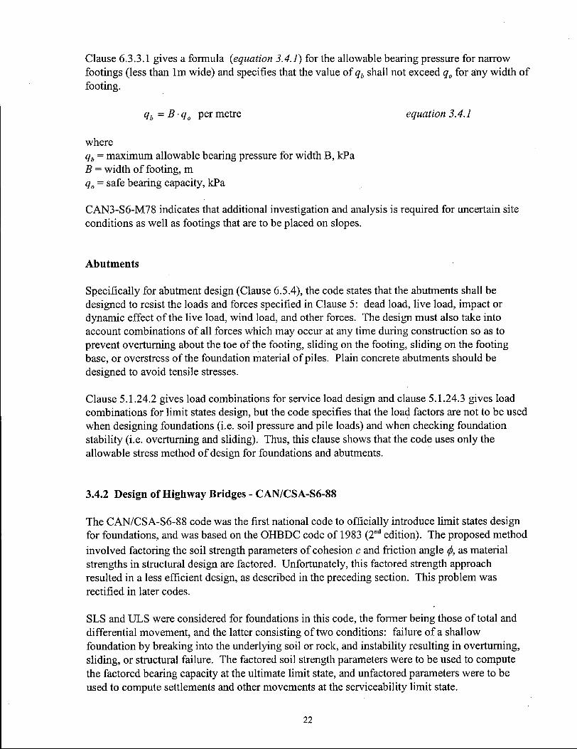
Clause 6.3.3.1 gives a formula {equation 3.4.1) for the allowable bearing pressure for narrow footings (less than l m wide) and specifies that the value of qb shall not exceed q0 for any width of footing.

qb = Bq0 per metre equation 3.4.1

where qb = maximum allowable bearing pressure for width B, kPa B = width of footing, m q0 = safe bearing capacity, kPa

CAN3-S6-M78 indicates that additional investigation and analysis is required for uncertain site conditions as well as footings that are to be placed on slopes.

Abutments

Specifically for abutment design (Clause 6.5.4), the code states that the abutments shall be designed to resist the loads and forces specified in Clause 5: dead load, live load, impact or dynamic effect of the live load, wind load, and other forces. The design must also take into account combinations of all forces which may occur at any time during construction so as to prevent overturning about the toe of the footing, sliding on the footing, sliding on the footing base, or overstress of the foundation material of piles. Plain concrete abutments should be designed to avoid tensile stresses.

Clause 5.1.24.2 gives load combinations for service load design and clause 5.1.24.3 gives load combinations for limit states design, but the code specifies that the load factors are not to be used when designing foundations (i.e. soil pressure and pile loads) and when checking foundation stability (i.e. overturning and sliding). Thus, this clause shows that the code uses only the allowable stress method of design for foundations and abutments.

3.4.2 Design of Highway Bridges - CAN/CSA-S6-88

The CAN/CSA-S6-88 code was the first national code to officially introduce limit states design for foundations, and was based on the OHBDC code of 1983 (2 n d edition). The proposed method involved factoring the soil strength parameters of cohesion c and friction angle <f>, as material strengths in structural design are factored. Unfortunately, this factored strength approach resulted in a less efficient design, as described in the preceding section. This problem was rectified in later codes.

SLS and ULS were considered for foundations in this code, the former being those of total and differential movement, and the latter consisting of two conditions: failure of a shallow foundation by breaking into the underlying soil or rock, and instability resulting in overturning, sliding, or structural failure. The factored soil strength parameters were to be used to compute the factored bearing capacity at the ultimate limit state, and unfactored parameters were to be used to compute settlements and other movements at the serviceability limit state.

22

The design of shallow foundations was to include consideration of the following: bearing capacity of the supporting medium at SLS and ULS, duration and distribution of loads, depth of the foundation, depth of anticipated scour, extent of frost penetration, possible ground movements, future dredging or excavation adjacent to the foundations, extent of seasonal volume changes in cohesive soil, proximity and depth of foundations of adjacent structures, and overall slope stability.

The structures are to resist all applicable loads as specified in Clause 5 on loads and forces. The 1988 code, as opposed to the 1978 code, does not specify unfactored loads for foundation design, except for serviceability limit states.

Bearing Capacity

Equations are given in Clause 6.6.2.3. of this code to calculate the bearing capacity at ultimate limit states. The notation used in the equations is explained in the text of S6-88.

a) Rectangular units with D/B > 2.5 placed on cohesive soils, and for all rectangular units placed on granular soils

qf = cf-Nc+yD-Nq+0.5-yB-Ny

b) For rectangular units with D/B<= 2.5 placed on cohesive soils equation 3.4.2

D + 5-c f 1 ^ (D) 1 n o B\ 1 + 0.2- — 1 + 0.2 • —

KB) \L) c) For square units placed on cohesive or granular soils

qf =l.2-cf -Nc + y-D-Nq +0A-y-B-Ny

d) For circular units placed on cohesive or granular soil qf =\.2-crNc+y-D-Nq+0.6-y-r-Ny

equation 3.4.3

equation 3.4.4

equation 3.4.5

The bearing capacity factors Nc, Nq, and Nr are given as functions of the modified angle of internal friction in S6-88 Figure 9. Factored bearing capacities for rock and unyielding soil are given in S6-88 Table 12. These are to be compared with the factored resistances as calculated with equations 3.4.2 - 3.4.5.

Specifications and suggestions are made for foundation materials with preferred failure planes, for distributing contact pressure, for inclined loads, and for shallow foundations on slopes.

Abutments

Section 6.8 in S6-88 deals specifically with piers, abutments, and retaining walls. The recommendations given with respect to abutments are: investigation of the overall stability of the soil mass underlying the structure, anchorage of foundations on smooth or inclined bedrock into the bedrock, and protection of the foundation from loss of ground support or lateral restraint, Abutment design should take into account all combinations of forces that may occur at any time

23

during construction, so as to prevent overturning, sliding, or overstress of the foundation material.

3.4.3 Canadian Highway Bridge Design Code - Draft 1998

The new draff code uses LSD as well, but uses a factored load and resistance approach as opposed to a factored strength approach. For shallow foundations, the values of factored geotechnical resistance at the ULS are determined. The factored geotechnical resistance is the ultimate geotechnical resistance multiplied by a resistance factor specified in the code (CHBDC Table 6-6.2.1). Different factors are given for various modes of failure of shallow foundations and deep foundations (based on similar factors from the OHBDC 1991). For example, the resistance factor for bearing resistance of a shallow foundation is 0.5, whereas the partial factor for sliding resistance is 0.8. C H B D C specifically states that foundation pressures at SLS for associated deformation values are to be based on calculations done with unfactored geotechnical parameters. SLS to be considered include both short term and long term differential settlements, as well as the simultaneous occurrence of several different types of deformation.

The code also states that the following failure modes must be considered alone, and in combination: overall stability of a foundation and any adjacent slope, bearing resistance, pull-out or uplift resistance, as well as sliding, horizontal shear resistance, and passive resistance.

Bearing Capacity

A formula is given for resistance at ULS for a concentrically loaded footing founded in deep uniform soil:

qu = c- Nc-sc-ic+q • Nq • sq -iq +0.5-/ • B- Ny • sy • iy equation 3.4.6

The values of the various coefficients and modifiers are explained in following sections of the code, as are changes required for situations with load inclination and eccentricity. Graphs and relationships are given for soil parameters varying with Nc, Ng, and NY.

3.5 Seismic Design

Canadian codes have typically not been used as guidelines for the seismic design of bridges in Canada. The 1988 code refers the reader to two different American codes for direction in this area - ATC-6 Seismic Design Guidelines for Highway Bridges and A A S H T O Guide Specifications for Seismic Design of Highway Bridges. However, the new draft C H B D C does address seismic design.

24

3.5.1 Earthquake Forces - C H B D C Draft 1998

Section 4 of this code deals specifically with seismic design and, in particular, Section 4.6 pertains to foundations. This section specifies that an evaluation should be made of the potential for liquefaction and suggests possible remediative measures. Slope stability and soil-structure interaction are also considered in this section of the code. However, it is only specified that an "analysis" should be performed, and no particular instructions are given. This leaves the extent of the analysis to the judgement of the engineer. The code mentions that seismically induced lateral soil pressures on the back of the abutment and retaining walls should be included when needed and suggests that these pressures can be calculated by the Mononobe-Okabe method.

3.5.2 A T C - 6 Seismic Design Guidelines for Highway Bridges (1983)

Chapter 6 of this code deals with foundation and abutment design requirements that are specifically related to seismic resistant construction. The bridge structure is assigned to a certain "seismic performance category" from A-D based on an acceleration coefficient (determined by geographic location) and is given an importance classification. Requirements are given for foundations and abutments in each category.

3.5.3 Standard Specifications for Highway Bridges ( A A S H T O 1989)

The earthquake section of this code refers the user to AASHTO Guide Specifications for Seismic Design of Highway Bridges (1983), but also gives a short list of analysis options to use. These include the equivalent static force method, the response spectrum method, and a short note on the design of restraining features. This section is not very detailed, as it is not expected to be used for design in a high seismic zone. The seismic design of foundations is not mentioned in this code.

3.5.4 ATC-32 Improved Seismic Design Criteria for California Bridges: Provisional Recommendations (1996)

The seismic design philosophy of ATC-32 for foundations consists of three main requirements. The first is that the foundation structure itself must be designed so as to prevent failure and achieve a preferred failure mode. Secondly, the bearing capacity of the foundation must be sufficient to prevent excessive settlements, and cyclic degradation effects should be included for earthquake loading conditions. The third requirement that must be satisfied is that of tolerable displacements. ATC-32 gives limiting guidelines of 0.008 radians and 2 inches for angular distortion and lateral deflection, respectively. It is noted that these values are only "conservative presumptive criteria" and higher values can be used based on the evaluation of a specific bridge.

Specific to abutment design, ATC-32 indicates that the capacity of the abutment to resist the inertial load of the bridge should be compatible with the structural design of the abutment wall, as well as the soil resistance. The soil capacity is to be evaluated on the basis of an applicable

25

passive earth-pressure theory, and also depends upon the soil resistance that can be reliably mobilised.

3.6 Summary

Although WSD is the traditional method of foundation design, the more recent codes are tending towards LSD for the conveniences and advantages presented in this chapter. The inception of LSD for foundation design in the new Canadian Highway Bridge Design Code wil l provide geotechnical engineers with more exposure to LSD methods. Since practice is guided by the codes, LSD will become more common once given the opportunity to be understood and accepted.

26

Chapter 4 . F L A C Model of Centrifuge Experiment

4.1 Introduction

In order to have confidence in a F L A C analysis of an abutment structure and embankment, it was necessary to model a case for which displacement and failure information was available. The C-CORE (Centre for Cold Ocean Resources Engineering) group at the Memorial University of Newfoundland (MUN) in St. John's, Newfoundland conducted a centrifuge study on a simple abutment structure. The C-CORE test involved loading to failure a simple bridge abutment founded on a sand embankment. Bearing loads and failure patterns were observed and documented (Randall, 1997), and thus allowed comparison with the results of a F L A C model. The F L A C model yielded comparable results in terms of failure load and displacement of the soil and structure. This agreement established F L A C as the basis for predicting response of full scale bridge abutments.

4.2 Centrifuge Theory

Centrifuge modelling involves accelerating a soil model at the end of a centrifuge such that the model is subjected to an inertial radial acceleration field. The model feels an acceleration that is many times stronger than that of the earth's gravitational field. The basic scaling law of centrifuge theory is that stress similarity is achieved at homologous points by acceleration of a model of scale N to N times earth's gravity (Taylor, 1995). Because soil behaviour is stress level dependent, a centrifuge allows one to test a model at appropriate stress levels.

One of the main advantages of centrifuge modelling is that correct distributions of stress and stress-strain behaviour (stress equality) can be achieved. There is a wide range of soil behaviour that is relevant to a particular geotechnical problem because of the changing insitu properties and stresses with depth, as well as the effects of varying soil layers. The centrifuge can represent the actual physical processes involved in a geotechnical problem by incorporating these issues into the model itself, and inducing a failure under controlled conditions (Craig, 1984). The centrifuge is very useful due to the proper replication of self-weight effects and generation of realistic failures. As opposed to other types of analysis, the mechanisms developed are not predetermined, but indicative of reality.

The centrifuge can be used to validate the use of numerical codes and analyses because of the realistic nature of stress and stress-strain distributions. Taylor (1995) reports that centrifuge test data have been found to give useful comparisons with detailed finite-element calculations. Ng, Springman, and Norrish (1998), concluded that centrifuge and numerical modelling techniques were effective in studying the behaviour of integral spread-base bridge abutments. They were able to identify rigid body motions and bending deflections of the abutment based on the experimental and numerical simulations of the prototype.

27

The two main issues in centrifuge modelling are: 1) the scaling laws used to convert parameters from the prototype to the model and 2) the scaling effects.

The scaling relationship for linear dimensions is 1 :N, when the model is subjected to an acceleration of Nxg. This can be illustrated by following the rule of stress equality. The stress in the model (model denoted by subscript m) is

o-vm=p-N-g- hm equation 4.1 The stress in the prototype (prototype denoted by subscript p) is

crvP= P'g-hp equation 4.2 where a- stress p = mass density g = earth's gravity N = scaling factor, and h = depth to which stress is to be calculated

For stress equality, cr^ = a^, and hp =N- hm equation 4.3

Hence, the scale factor for linear dimensions has been shown to be 1 :N. Thus, displacements have a scale factor of 1 :N, and strains have a scale factor of 1:1. The scale factors for other parameters are presented in Table 4.2.1.

Table 4.2.1 Scale Factors for Centrifu; Parameter I Prototype acceleration

density force

friction angle length mass strain stress

ge Experiments Model

N

1/N2

1/N 1/N3

1

The validity of the modelling procedure can be checked using the concept of "modelling of models". This involves testing a variety of models of the same prototype at different scales and comparing the results. Similar results indicate successful modelling, as shown by Gemperline and Ko (1984).

4.3 The Experiment

The prototype for the centrifuge experiment is an existing abutment in a bridge near Toronto, Ontario. Detailed information on the model, procedures, and results is presented by Randall (1997). The key features of the experiment that are important for developing a comparative

28

model in F L A C are: model dimensions, soil properties, level of acceleration, failure load, and displacements.

The centrifuge model was scaled down 1/70 of the size of the prototype structure. The dimensions of the prototype and the experimental model are presented in Table 4.3.1. The scaling factor, N , is 70 as dictated by the acceleration of the centrifuge model. A l l linear dimensions are scaled directly by a factor of 70, as discussed in section 4.2.

Table 4.3.1 Prototype and Model Dimensions. Parameter Prototype Model

footing height 5.8 m 82.9 mm footing thickness 0.9 m 12.9 mm

footing width 3.8 m 54.3 mm slope height 11.6m 165 mm

length of abutment 21 m 288 mm gravity 70g l g

The sample was prepared by raining sand into a special "plane strain" box. The sand was unsaturated, and not compacted by any means other than preparation. The soil properties were defined by tests conducted at C-CORE for previous experiments. The sand chosen was glass sand, which was used in the Northumberland Straight Crossing tests. Test results show that the friction angle varied between 29.1° and 40.7°, and the dry unit weight varied between 12.65 kN/m 3 and 15.79 kN/m 3.

A n additional load was applied to the top of the abutment with a hydraulic actuator. The purpose of this was to simulate the superstructure load. The sample was then accelerated to 70g to represent the required level of acceleration for a model of this scale. The resulting failure load was 19.6 k N over a width of 0.288 m which is equivalent to a load of 68.1 k N over 1 m. The maximum vertical displacement measured at the top of the abutment was 3.4 mm.

The C-CORE experimental result was compared to theoretical values of bearing capacity by Meyerhof, Terzaghi, Vesic, and Hansen. Table 11-1 "Results of Ultimate Load Capacity for Centrifuge Test and Case Studies" in Randall's paper presents some dubious values for Case 5 (that being the case most similar to the experimental situation). The values were recalculated and the results were closer to the ultimate load capacity of 96 M N found in the centrifuge experiment. The resulting values are tabulated with Randall's values for direct comparison (Table 4.3.2). Recall that (P u l t ) m o d e l = l /N 2 (P u l t ) p r o t o t y p e , where N , the scaling factor, is equal to 70. Thus, for a (P u l t ) p r o t o t y p e = 96 M N , the (P u l t ) m o d e l = 19.6 kN, which is equivalent to the value predicted in the experiment.

Table 4.3.2 Ultimate Load Capacity (MN) for Prototype C - C O R E paper Recalculation

Terzaghi 271 96 Meyerhof 349 93 Hansen 213 72 Vesic - 117 Measured 96 -

29

Gemperline and Ko (1984) conducted a series of centrifuge tests on bridge footings constructed at the crest of a steep slope. These tests were very similar in manner to the test carried out at C-CORE. The model was of a similar scale with 76 mm to 152 mm slope heights and 13 mm to 26 mm footing widths. Other similarities included the following: the footing was on a steep slope of 1.5H: 1V (C-CORE was 2H: 1V), the material used in the test was air-dried sand poured in lifts, and the slopes were prepared by vacuuming and hand-trimming. The main differences were that the footing was constructed of aluminium, and that a flight of scale factors was used., as opposed to the single scale factor of 70 used in the C-CORE test.

Gemperline and Ko applied the concept of "modelling of models" to ensure that the footing was successfully modelled. Scale factors of 50, 66.7, and 100 were used in various tests and the results compared to each other using the scaling laws. The results of the experiments were evaluated against theoretical analyses of bearing capacity. The methods that were validated by the centrifuge experiment were those of: Kusakabe, Meyerhof, Hansen, and Giroud, as well as the Spencer Limiting Equilibrium Approach. It was found that these methods can be used with the plane strain friction angle and standard bearing capacity safety factors to predict safe allowable bearing pressures.

Good results in Gemperline and Ko's comparisons with standard bearing capacity theories increase confidence in the accuracy of the C-CORE modelling due to the apparent similarities in the experimental methods. Additional verification by Gemperline and Ko with the "modelling of models" procedure gives assurance that the results of the C-CORE tests are reasonable. In addition, both experiments concluded that the Meyerhof and Hansen bearing capacity theories (Bowles, 1996) predict realistic values of bearing pressure when compared to centrifuge tests.

4.4 F L A C Model

The F L A C model was developed to compare with the results of the centrifuge test, and so the experimental parameters were used as opposed to the dimensions of the real-life structure. In addition, the gravity specified in F L A C was 70g - the level experienced by the model throughout the course of the experiment. The soil properties required for the F L A C model were taken from the tests done on the glass sand at C-CORE. Density, friction angle, shear modulus, and bulk modulus were determined based on the average of values discussed in section 4.3. The values used for density and friction were 14.7 kN/m 3, and 38° respectively. A Young's modulus of 9500 kPa was calculated on the basis of a drained triaxial compression test with a cell pressure of 275 kPa. Using a Poisson's Ratio of 1/3, initial values of shear modulus (G) and bulk modulus (B) were calculated to be 3500 kPa and 9500 kPa, respectively, based on the following relationships:

G = ^ -2(1 + / / )

B = ^ — 3 0 - 2 / / )

The values of moduli were modified to attain a good correlation between the centrifuge experiment and the F L A C model. The final values selected for use in the analysis were a shear

equation 4.4

equation 4.5

30

modulus of 4000 kPa and a bulk modulus of 9000 kPa. These values were only a starting point, as the moduli were set to vary with stress in the abutment embankment (Seed, 1985). The maximum value of shear modulus (G m a x) was calculated for each element as:

G m a x = 440 • (w, C -Pa-pr e < l u a t i o n 4 - 6

where: f Veo = the corrected value of number of blow counts from a standard penetration test P a = atmospheric pressure (100 kPa), and crm = mean stress.

The value of (N,) 6 0 was based on the relative density (D r= 83%) reported by Randall (1997). Using correlations with cone penetration values (Campanella et al. 1995), an estimated value of 27 was determined for (N,) 6 0. The shear modulus was set to 0.1 x G m a x , and the bulk modulus was set to 0.3 x G m a x for each element of the F L A C mesh. As a result, the moduli vary with the stresses in the model and range from 4000 to 20000 kPa for shear modulus and 9000 kPa to 50000 kPa for bulk modulus.

The undeformed grid with the abutment modelled as structural elements can be seen in Figure 4.4.1.

FLAC (Version 3.40)

12-JUI-99 9:14 step 0

-5.000E-02 <x< 9.500E-01 -3.800E-01 <y< 6.200E-01

Grid plot

Beam plot

MoTH Geotechnical British Columbia

0.200 0.300 0.400 0.500 0.600 0.700

Figure 4.4.1 Undeformed F L A C grid of centrifuge experiment.

4.5 Comparison of Centrifuge Experiment and F L A C Model

The accuracy of the F L A C model was determined on the basis of maximum displacement and failure load. Table 4.5.1 shows the experimental results and the F L A C results. The failure load

31

applied in the experiment was 19.6 kN over a width of 0.288 m. This is equivalent to a load of 68.1 k N over 1 m. The F L A C analysis is a 2-D plane strain problem, with all values determined for a unit width. Displacements were measured at the top of the abutment, in both the experiment and F L A C model.

From this comparison, it can be seen that the F L A C model showed good agreement with the centrifuge experiment.

Table 4.5.1 Results of centrifuge experiment and F L A C model of experiment. Experiment F L A C model

Displacement (mm) 3.4 3.1 Failure Load (MN) 68.1 65.3

Also of note are the failure patterns of the experiment and F L A C model. A picture of the experimental model after failure is shown in Figure 4.5.1, and Figure 4.5.2 is the deformed F L A C mesh. Comparing these figures shows that the F L A C model failed in the same fashion as the centrifuge model. The F L A C input file can be viewed in Appendix A .

3 2

J O B T ITLE :

FLAC (Version 3.40)

L E G E N D

27-Aug-98 '12:05 step 132500

-5.000E-02 <x< 9.500E-01 -3.799E-01 <y< 6.201 E-01

Exaggerated Grid Distortion Magnification = 5.000E+00 Max Disp = 6.652E-03

M o T H Geotechnical British Columbia

Figure 4.5.2 Deformed F L A C mesh after failure.

33

Chapter 5. No. 5 Road Overpass Abutment - WSD and L S D

5.1 Introduction and Background

The No. 5 Road overpass abutments were designed using WSD in 1985, and the overpass structure was built in 1986. The structure carries traffic on the Richmond East-West Freeway over the No. 5 Road at a point approximately midway between Cambie Road and the New Westminster Highway. The overpass has three simply supported spans of 12, 19, and 12 m respectively. The design is the same for both east and west abutments due to the symmetry of the overpass, and the fixidity conditions at the piers. The spans are fixed at the piers and horizontal movement on bearings is allowed at the abutments. The structure was constructed to withstand the 475 year earthquake, corresponding to a peak firm ground horizontal acceleration of 0.2g (Fraser, 1985). Restrainer bolts are provided at the abutments to limit the horizontal displacements during an earthquake event.

A site investigation was carried out to provide information on soil stratigraphy. Four static cone penetration tests (CPT) were conducted and the resulting soil profile is shown in Figure 5.1.1

Depth (m)

0 x X 7

soft to firm organic silt and clay

-2

layered sandy silt and silty sand

-5

compact to dense sand

-24

firm to stiff silt and clay with sand layers

Figure 5.1.1. Soil Profile from CPT

Design recommendations included excavation of the organic soils (to -2 m), and densification of the insitu sand layer and backfill by vibro-replacement techniques. The sand was to be densified to the following criteria: 1) above 10 m q c = 10 Mpa 2) below 10 m q c > 10 + (depth - 10) Mpa where q c is the tip resistance of the static electric cone. The densification was specified to extend 10 meters beyond the toe of the bridge end fill , and 10 m from the centerline of the pile caps for the piers. The vertical extent of the densification was

34

to be from the water table (elevation 0) to a depth of 16 m. Liquefaction was not a consideration for this analysis. It was assumed that the soil densification was sufficient and that the embankment was constructed within specified guidelines so as to prevent liquefiable soil conditions.

The ultimate bearing capacity for the spread footings was estimated to be 600 kPa, and a factor of safety of 3.0 was recommended for normal working loads. It was assumed that Fraser River Sand was used for the bridge end fill, and the footings were recommended to be set back a minimum of 1.5 times the footing width from the face of the 1.5H:1V sideslopes. It was also noted that the factor of safety may be reduced when considering the maximum contact pressure under extreme seismic loads.

5.2 Working Stress Design

The working stress design for the No. 5 Road overpass abutment was done at M o T H in October of 1985 using the CAN3-S6-78 Code. Four cases were checked:

1) Dead load of the substructure + earth pressure 2) Dead load of substructure + dead load of superstructure + live load of the superstructure +

earth pressure, (bearing pressure check with service loads) 3) Dead load of superstructure + dead load of substructure + restrainer earthquake forces (no

live load) 4) Seismic soil forces in accordance with the AASHTO Seismic Code (1983)

The Factors of Safety (FS) for each case in terms of overturning and sliding were determined as follows:

FS overling = ^ ^ " a b " a m g equation 5.2.1

overturning

pSsliding = - ^ T ; — equation 5.2.2

where:

M = moment about the toe ju = Poisson's ratio Fy = vertical force, and FH = horizontal force.

Reinforcement design for the footing, pedestal wall, ballast wall, and wingwalls is also detailed in these calculations, along with miscellaneous details such as hold-down bolts and earthquake restrainer bolts.

The cases introduced above are described in more detail in the subsequent sections and the original design calculations can be viewed in Appendix B.

35

5.2.1 Case 1

Case one was a stability check with the service loads. This calculation was done to check the stability of the abutment prior to the erection of the superstructure. Grade I loads of 100% were used. To be conservative, it was assumed that the wingwall was built prior to erection, and the soil in front of the wall was neglected.

5.2.2 Case 2

Case two included the superstructure load. The dead load portion of the superstructure was comprised of the loads from components such as the slab, stringers, haunch, parapets, and median. The live load accounted for 4 lanes of traffic, with 346 kN per lane, and a 75% reduction. The resulting dead and live loads per linear meter of abutment were 56.8 k N and 45.1 kN respectively. The resultant of the vertical loads was found to be in the middle third of the abutment, and the bearing pressure was confirmed as less than the allowable value of 200 kPa. Thus, it was concluded that the abutment satisfied overturning and sliding requirements for this case. This case was also a serviceability check and used Grade I loads of 100 % (service loads).

5.2.3 Case 3

Case three considered the earthquake restrainer force on the substructure. The restrainer design force was determined based on the AASHTO Seismic Code (1983), and was equivalent to an acceleration coefficient x the weight of the span. In this case, the value was 23.7 kN per linear m of the abutment. The dead load in this case included the weight of the diaphragm, and thus was 61.8 kN/m.

5.2.4 Case 4

The seismic soil forces were determined using the pseudo-static Mononobe-Okabe analysis recommended in the A A S H T O Seismic Code (1983). This method uses unwieldy empirical equations based on friction angle, unit weight, acceleration coefficients, and the geometry of the retained soil to calculate active earth pressures. The Grade 7 load combination of Dead Load + Earth Pressure + Earthquake Load (DL + E + Q) governed, and factored loads were used (i.e. 1.3(DL + E + Q)). The maximum bearing pressure was 507 kPa, which is less than the ultimate bearing capacity of 200 kPa x 3 = 600 kPa. However, the resultant of the vertical loads was found to be outside the middle third of the base. Design notes indicate that this ultimate value should be used with discretion, but that a slight exceedance of average ultimate capacity is allowed. The FS values are low, but were considered to be adequate for the infrequent earthquake condition.

5.2.5 Factors of Safety for WSD

The resulting values of FS for the WSD from the MoTH calculations are listed in Table 5.2.1. The low values for Case 1 sliding and Case 4 are accepted since they are temporary or low

36

probability conditions. It is common to require a lower factor of safety for earthquake conditions and erection cases.

Table 5.2.1 Factors of Safety for WSD from MoTH calculations Overturning Sliding

Case 1 2.41 1.13 Case 2 "ok" "ok" Case 3 1.74 1.3 Case 4 1.27 1.15

5.3 Limit States Design

The LSD method of the CHBDC draft was applied to the No 5 Road overpass abutment in order to facilitate a comparison between LSD and WSD. The procedure involves determining the geotechnical resistance (for different failure modes) of the structure, and then comparing this value to the appropriate factored loads as outlined by Section 3 of the CHBDC.

The partial factors for various geotechnical resistances are given in Table 6-6.2.1 of the CHBDC, and those for shallow foundations have been repeated in Table 5.3.1.

Table 5.3.1. Geotechnical Resistance Factors for Shallow Foundations Type of Resistance Factor

Bearing Resistance 0.5 Passive Resistance 0.5 Horizontal Resistance (Sliding) 0.8

Bearing and horizontal resistance were checked with LSD, with two main load combinations being investigated. These particular combinations were chosen because they are similar to the load cases used in the WSD. The combinations considered for ULS were ULS 1 and ULS 5 in the C H B D C . The first is a combination of dead load, earth loads, and live loads, and the second combination involves dead loads, earth loads, and earthquake loads (equations 5.3.1 and 5.3.2).

ULSl = aD • D + aE • E +1.70 • L equation 5.3.1

ULS5-aD-D + a E E + \.0EQ equation 5.3.2

where: D = dead load E = earth load L = live load EQ = earthquake load au = load factor on dead load GCE = load factor on earth load.

The load factors depend on the type of loading, and were taken from Table 3.5.1(b) in the CHBDC. The factors used in the analysis are given in Table 5.3.2.

37

Table 5.3.2. Load factors from CHBDC Dead Load aD

Cast-in-place concrete, wood, and all non-structural components 1.2 Earth fill , negative skin friction on piles 1.25

Dead Load in Combination with Earthquakes A l l dead loads for ULS 5 1.25

Earth Pressure and Hydrostatic Pressure Passive earth pressure, considered as a load 1.25 At-rest earth pressure 1.25 Active earth pressure 1.25 Backfill pressure 1.25

5.3.1 Loads

The live load transferred to the abutment was calculated in accordance with the specifications in the C H B D C . The standard truck (CL-625) was used for the truck load, and the lane load was 80% of the truck load plus a uniform lane load of 9 kN/m. The governing result was a live load of 37 kN per linear m of the abutment due to the lane loading. This is less than the load of 45.1 kN/m used in the WSD due to the different number of design lanes used (see Appendix B for calculations). The dead load for the abutment structure was calculated based on weight of the concrete and earth fill with the appropriate load factors applied to each component of dead load. The unit weight of concrete used was 23.5 kN/m 3 , as taken from C H B D C Table 3.6. A unit weight of 19 kN/m 3 and a friction angle of 33° were used for earth pressure calculations. The values of these parameters are the same as those used in the WSD calculations for consistency and comparison. Horizontal loads from the superstructure were not considered because the bearings on the abutment seat allow horizontal movement.

The superstructure dead load of 56.8 kN/m was taken from the MoTH WSD. Active and passive pressures were calculated using Coulomb theory. Coulomb's equations for K A and Kp, the active and passive earth pressure coefficients, were used. For seismic response, the Mononobe-Okabe method was used to calculate the total active and passive thrust due to earthquake loading.

The earthquake restrainer force was calculated based on section 4.4.10.6 of the C H B D C . It is specified that the restrainers should be designed for a force equal to 3 times the Zonal Acceleration Ratio (A) multiplied by the dead load of the lighter of the two adjoining spans or parts of the structure. The weights of the adjoining span, as well as the abutment structure itself were considered, and the abutment was found to be lighter. The resulting restrainer force for an A value of 0.20 (which corresponds to a PHA of 0.21 g) was calculated to be 54.5 kN/m. This value is significantly higher than the restrainer force used in WSD which used A A S H T O specifications.

The height of the abutment structure varies along its length, and so the two extremes (minimum and maximum soil depth) were investigated. A surcharge of 600 mm depth is also applied in the WSD. This was included only to give a more conservative estimate of response, and was not considered for the case of earthquake loading.

38

5.3.2 Bearing Capacity

ULS 1 and SLS were considered for bearing capacity. A seismic check on bearing resistance was not performed because the principal loading by an earthquake is in the horizontal direction. For ULS 1 the minimum factored load was 271.0 kN/m for a soil depth of 3.52 m, and the maximum factored load was 299.9 kN/m for a soil depth of 4.02m. These values correspond to linear and uniform pressure distributions as shown in Figure 5.3.1. Maximum values of the resistances were used for comparison to the factored loads.

Minimum Soil Level

86 kPa 160 kPa 123 kPa

Maximum Soil Level

99 kPa

174 kPa 136 kPa

Figure 5.3.1. Factored Pressure Distributions of Loading

The following relationship is given in Section 6 (Foundations) of the C H B D C for bearing capacity (see also Bowles, 1996). The draft version of CHBDC used for this analysis does not specify the source of the relationship, or of the required factors. The factors are supplied in poorly reproduced charts without references or equations. It would be helpful to supply references, or perhaps more useful graphs and/or equations for the factors.

(lu=c-N c-sc- ic +q -Nq-sq- iq + 0.5 • y • B • Ny • sy • iy equation 5.3.3

In any case, the formulation and charts are similar to methods outlined by Bowles (1996), and it is suspected that the factors used are those specified by Terzaghi. This equation can be simplified since the soil is cohesionless (c = 0), and because it is a strip footing-like problem where the shape factors sc = sq = sY= 1.0. With these simplifications, the working equation becomes:

qu=q'Nqiq+0.5yBNyiy equation 5.3.4

From Figure 6-7.3c in the CHBDC, values for N y and N q were found to be 22 and 23, respectively. The width of the base is 2.2 m and the unit weight used in the calculations was 19 kN/m . However, q', i q and i Y depend on the soil depth which was taken as 3.52 m in the minimum soil level case, and as 4.02 m when the soil depth is maximum. The resulting factored and unfactored resistances are tabulated with the loads in Table 5.3.3

39

Table 5.3.3 Comparison of Factored Load and Factored Resistance for Bearing Resistance Factored Factored

Soil Level (kPa) Resistance (kPa) Load (kPa) Minimum 1562 781 > 160 Maximum 1652 826 > 174

Note that the factored resistance in both cases is about 4.8 times the factored load. This could indicate a structure that is overdesigned, but more likely shows that ULS do not usually govern in foundation design. The more critical check is that of SLS.

The SLS were checked based on estimates of elastic settlements of shallow foundations, as outlined by Becker (1998).

„ q • B v = ~ ^ — e q u a t i o n 5.3.5

A n insitu Young's Modulus value of 20 000 kPa was chosen for the sand based on equations 5.3.5-7, and on tabulated values in Bowles (1996). The influence coefficient, I, was taken as 0.88 from Figure 12.2 (after Kany, 1959) in the Canadian Foundation Engineering Manual (1992).

£ = 8 0 0 0 ^ ^ 7 equation 5.3.6

Ex = 2qc —» 4qc equation 5.3.7

Es = 500 • (N +15) equation 5.3.8

The equation was calculated for a number of displacements, 5, and bearing pressures, q (Figure 5.3.2). If the SLS displacement is specified to be a minimum of 18 mm, the corresponding bearing resistance would have to be 186 kPa. As the maximum loading is 180 kPa, this is the lowest displacement criteria that can be specified, and still have the system pass the SLS criteria. For example, i f the displacements were specified to be no less than 20 mm, the corresponding resistance would be 207 kPa, and the design would be sufficient. However, i f the maximum settlement was to be limited to 15 mm, the resistance would be only 155 kPa, and the system would not meet this criteria. Expected displacements in mm, according to A A S H T O Seismic Guidelines (1983) are in the order of 254 x PGA. In this case, the PGA is 0.21g, and so the outward displacement of the abutment can be expected to reach 53 mm, and should be designed for this. Allowing the abutment to displace 53 mm would mean that it would be able to take a load of up to around 500 kPa. This is definitely greater than the expected loading of 180 kPa, and so the system would meet the SLS criteria.

40

S L S - Elastic Settlements of Shal low F o u n d a t i o n s

ro £ 6 0 0

tx

4 0 0

2 0 0

q = 5 E s / B I

\

\ | re sista nee = • 186 kPa |

0 2 0 4 0 6 0 8 0 1 0 0

D i s p l a c e m e n t - g (mm)

Figure 5 . 3 . 2 . SLS elastic settlement criteria

Personal communication with engineers at MoTH (Gillespie and Szto, 1 9 9 9 ) resulted in some guidelines for maximum allowable post-earthquake displacements of the bridge abutment. The vertical limit was said to be around 3 0 0 mm, after which point, repairs would become expensive and would require more than jacking or additional fill. Longitudinal movements should be less than the seat width minus 1 0 0 mm. In this case, the limiting value would be 7 5 0 mm. These magnitudes of displacements would be next to impossible to achieve without liquefaction and so are not of concern in this design (assuming the structure was constructed as specified).

5.3.3 Sliding Resistance

The horizontal resistance of the abutment was calculated using the relationships given in Section 6 - 7 . 6 of the CHBDC. The horizontal resistance was taken as the lesser of the resistance due to the shear resistance of the soil (H r s), or due to the shear resistance at the interface between the structure and soil (Hrj).

Hrs = 0 .8v4 • c' + 0Wf tan^' equation 5.3.9

Hri = 0 . 8 , 4 • c' + 0Wf tanS equation 5.3.10

Wall friction, S, was based on information tabulated by Kramer ( 1 9 9 6 ) and a value of 2 2 ° was assumed. As in the bearing capacity equations, the soil was specified to be cohesionless, and the friction angle ( $ used was 3 3 ° . The vertical forces, Vf, included the weight of the substructure, the weight of earth fill bearing vertically on the footing, and the weight of the superstructure. The sliding resistance was also checked without the weight of the superstructure (for the case of a stand-alone abutment, before the bridge is completed). The factored resistance was calculated with and without the passive resistance of the soil in front of the abutment, and all results are given in Table 5 . 3 . 4 . Passive pressures included in the resistance were modified by the specified factor of 0 . 5 , and were calculated using the relationships (based on Coulomb theory) in equations 5 . 3 . 1 1 and 5 . 3 . 1 2 (Terzaghi, 1 9 5 4 ) . The results of the calculations are shown only for the

41

minimum soil level case, which is the more conservative. It is noted that this equation may produce unsafe values when 8 is less than 0/3. However, the passive pressure is included just for comparison purposes, and is not relied upon to meet LSD criteria. The angles a and /?rely on the geometry of the system and are 90° and 0 ° , respectively.

KP = sin 2 (or -0)- cos 8

sin a • sm(a + 8)

Pv=-Kv-yW

1 -sin(0 + 8) • sin(0 + B) sin(a + 8) • s\n(a + B)

equation 5.3.11

equation 5.3.12

The loading case of ULS 1 can be reduced to the following equation because there are no horizontal dead or live loads on the structure due to the fixidity conditions at the abutment.

Load = 1.25-PA equation 5.3.13

The active pressure, PA , for the minimum soil level is 31.1 kN/m. The coefficient of minimum active earth pressure, K A , is determined based on Coulomb theory ( N A V F A C , 1982), and PA is

PA=±KA-/-H2

cos2 (0-0)

cos2 6-cos(8 + 0) 1 + sm(8 + 0) • sin(0 - fp) cos(J + 0)-cos(0-/?)

equation 5.3.14

j equation 5.3.15

The angles 0 and B depend on the geometry of the system, and in this case, both are equal to zero. The factored load is shown with the resistances in Table 5.3.4.

Table 5.3.4. Factored Loads and Resistances for Horizontal Sliding - ULS 1

Factored Resistance (kN/m)

Factored Load (kN/m)

Substructure + Surcharge 38.6 < 53.3

Substructure + Surcharge +

Passive Resistance 103.6 > 53.3

Substructure 37.2 < 38.9

Substructure + Superstructure 55.5 > 38.9

Substructure + Passive Resistance 102.2 > 38.9

Substructure + Superstructure +

Passive Resistance 120.5 > 38.9

42

The results of the analysis indicate that the structure is safe against sliding when the complete structure has been erected. The surcharge creates additional load, and makes the situation more extreme. However, this is a temporary case which occurs only during construction, and so is not of concern in the overall performance of the structure during its lifetime. The structure is stable even when passive pressure is not included, but the factored resistance becomes up to 3 times the factored load when passive pressure is considered. Again, this may indicate an overdesigned structure, as the vertical forces would decrease with a decrease in weight (i.e. size) of the abutment structure. A decrease in vertical force reduces the resistance directly.

The earthquake forces were considered using ULS 5 where the load is defined as:

Load = 1.25PA +1 .OEQ +1 .OAP AE equation 5.3.16

The restrainer force, E Q , as described earlier in Section 5.3.1. had a value of 54.5 kN/m. The additional earth force due to an earthquake, A P A E , was determined using the Mononobe-Okabe (M-O) method (equations 5.3.15-17) as suggested in the CHBDC. A horizontal pseudo-static acceleration kh of 0.1 g was assumed, and the vertical component, k v, was taken to be 0.

PAE = 1

•KA,ryH\\-kv) equation 5.3.17

K AE cos {(/> - 9 - y/)

cos y/ • cos 9 • cos(<J + 9 + y/)- 1 + sin(<J + <j>) • sin(0 - j3 - y/)

cos (£ + 9 + y/) • cos(/? - 9)

equation 5.3.18

y/ - tan" equation 5.3.19

The active earth pressure can be divided into two components - a static component, P A , and a dynamic component, APAE-

PAE =PA+ &PAE equation 5.3.20

These two components were factored separately, in accordance with equation 5.3.14. Two sets of vertical forces were considered for this ULS, the first being the weight of the abutment and the vertically bearing soil, and the second including also the weight of the superstructure. Passive pressure was determined by the M - 0 method as well when considered for the earthquake case (equations 5.3.21 - 5.3.23).

PPE=\-KPE.yH\\-kv) equation 5.3.21

K PE cos {<j> + 9 - y/)

cosy/ • cos 9 • cos(<5-9 + y/)-s'm{S + </>) • sin((zi + (5 - y/)

' cos(<5 - 9 + y/) • cos(/? - 9)

equation 5.3.22

43

PPE=Pp+APf equation 5.3.23

The passive pressure in this case is reduced by the dynamic component, APPE , to determine the passive earthquake resistance, PPE. This value is also reduced by the factor of 0.5, as it was in the static case.

Comparisons between factored load and resistance are shown in Table 5.3.5 for the various combinations of loads and resistances. The low value of resistance in the first case is of little concern, as the probability of an earthquake occurring during the time it takes to construct the bridge is much less than the probability of occurrence of an earthquake throughout the life of the structure. The ratio of factored resistance to factored load in this case is approximately 1.18 for the governing cases (i.e. superstructure + substructure and substructure + superstructure + restrainer force + passive resistance). This is still indicating a slight overdesign of the structure, but it must be kept in mind that the passive resistance is necessary in the case where the restrainer force is considered. The limiting cases of ULS 1 do not rely on passive resistance, whereas the earthquake case (ULS 5) does.

Table 5.3.5 Factored Loads and Resistances for Horizontal Sliding - ULS 5 Factored

Resistance (kN/m) Factored

Load (kN/m) Substructure 37.2 < 46.5

Substructure + Superstructure 55.5 > 46.5

Substructure + Passive Resistance

101.1 > 46.5

Substructure + Superstructure + Passive Resistance

119.4 > 46.5

Substructure + Superstructure + Restrainer Force + Passive

Resistance 119.4 > 101.0

5.4 Comparison of WSD and L S D Results

In order to directly compare the results from WSD and LSD, a ratio was determined for the LSD results in keeping with the basic idea of safety factors (i.e. the ratio of capacity to demand). Thus, the LSD ratio used is simply the factored resistance divided by the factored load. Recall that when applying LSD, the main goal is to have a factored resistance that is greater than or equal to the factored load. Thus, the calculated LSD ratio need only be one or greater. As the value increases from one, the design becomes more reliable. This concept can be compared to the familiar WSD FS in which the target value is something greater than one. A value of one indicates failure in WSD, and not safety as in LSD.

With this comparison strategy, i f the two design methods resulted in structures that were equivalently reliable, the value of the LSD ratio would be less than the traditional WSD FS. This would be due to the fact that the reliability issue had already been accounted for in LSD with partial factors on the load and resistance.

4 4

Interestingly, this is not the case. In looking at bearing and sliding (Table 5.4.1), it can be seen that not only are the LSD ratios greater than one, but they are also higher than the WSD FS. This indicates that the initial design (as developed using WSD) could have been more efficient i f it had been designed using LSD as outlined in the CHBDC. The large differences between factored strength and factored resistance could be adjusted and rechecked when using LSD as a design tool. According to these results, LSD would have resulted in a smaller abutment i f the geometry of the system would have allowed it.

Table 5.4.1 LSD ratios vs. WSD FS

Bearing Sliding Bearing Static (M-O)

WSD FS 3.9 1.13 1.15 L S D ratios 4.8 1.43 1.19

This comparison is valid only for this particular structure. Before conclusions are made as to the relative efficiency of LSD as opposed to WSD, more structures should be investigated in this manner.

45

Chapter 6. Determination of Reliability Index for No. 5 Road Bridge Abutment

6.1 Introduction

Soil properties tend to vary within a region and are often difficult to characterise. In general, even i f the soil type is known, the values of the strength and stiffness parameters to be used in analysis are not immediately apparent. Many geotechnical correlations and empirical relationships have been developed to accommodate for this lack of information. However, other methods, such as the reliability analysis presented in this chapter, can also be used to account for the uncertainties involved in geotechnical design.

The abutments for the No. 5 Road Bridge are founded on a fill of Fraser River sand. Because this material is relatively uniform, the properties can be estimated within a certain range. A finite difference model was developed to determine the behaviour of this particular soil-structure under bridge loading. The soil properties input to the model were randomised as normal distributions throughout the soil mass for a number of simulations. In each case, the capacity of the abutment was determined by applying a series of loads and noting the point of failure. The resulting individual capacities were fit to a normal distribution that described the capacity of the abutment structure.

The demand on the abutment structure was represented by probabilistic models for the dead and live load portions of the loading. Dead load was represented by a normal distribution, and the live load was represented by a Gumbel extreme distribution.

A first order reliability method (FORM) was then applied using the program R E L A N described in Chapter 2. This allowed the reliability index, B, to be determined and compared for a range of mean live loads.

46

6.2 Capacity determined by F L A C

The capacity of the abutment was determined by modelling the abutment and fill with F L A C (Itasca, 1998). A 73 x 32 grid was developed, and the necessary parameters were assigned to the appropriate grid locations to represent the abutment and the soil (see Figure 6.2.1).

JOB TITLE :

FLAC (Version 3.40)

LEGEND

13-JUI-99 14:51 step 0 -4.971 E-01 <x< 1.424E+01 -4.367E+00 <y< 1.037E+01

Grid plot I.., I I

0 2E 0

MoTH Geotechnical British Columbia

V Q

0.500 0.700 0.900 <M0«1)

Figure 6.2.1 Undeformed mesh of No. 5 Road bridge abutment

The soil and concrete abutment were modelled as elastic-plastic materials with the strength in accordance with Mohr-Coulomb criterion. The required elastic parameters are the bulk and shear modulus, and the plastic parameters are the cohesion and friction angle. The properties assigned to the concrete abutment were: shear and bulk modulus = 1x10s kPa, density = 2500 kg/m3, friction = 45°, and cohesion = 1000 kPa.

The friction angle and density of soil were specified as normal variables with means of 36° and 1800 kg/m3 and standard deviations of 2° and 100 kg/m3 respectively. F L A C has an intrinsic function (rdev) that can be used to assign random values of the specified properties (i.e. friction and density) to the grid elements in accordance with a normal distribution. Figure 6.2.2 shows the effect of this function by displaying contours of density throughout the grid.

47

JOB TfTLE :

FLAC (Version 3.40)

13-Jul-99 14:53 step 0 -4.971 E-01 <x< 1.424E+01 -4.367E+00 <y< 1.037E+01

Density Contour interval 1 .OOE-01 Mnimum: 1.50E+00 Maximum: 2.40E+00 Boundary plot

ul

2E 0

MoTH Geotechnical British Columbia

0 . 7 0 0 C O - ' )

Figure 6.2.2 Density contours in the mesh after rdev is applied

The shear and bulk moduli of the soil were defined as functions of (N,) 6 0 and overburden stress (equation 2.3.2). The value of (N,)6 0was set as a normal random variable with a mean of 12 and a standard deviation of 3. The variation of (N,) 6 0 as well as the functions to determine the moduli were defined using FISH, which is the coding language of F L A C . A sample input file, along with FISH functions can be found in Appendix C. The coefficients of variation (covx, equation 6.1) for these random variables fall within the ranges reported by Becker (1996). See Table 6.2.1 for comparisons.

<jx cov x = equation 6.1 X

where ax is the standard deviation of X , and X is the mean value of X .

Table 6.2.1 Coefficients of Variation for Random Variables Range of cov (Becker) cov Values Used

Unit Weight 0.04-0.16 0.06 S P T N 0.15-0.50 0.25

Friction Angle 0.05-0.25 0.06

A n incremental load (from 0 to 190 kN) was applied to the abutment, and load (P) vs. displacement (8) curves were developed to determine the capacity of the system. The shape of the deformed system and the displacement vectors are shown in Figure 6.2.3. Capacity was chosen as the apparent "yield point" of the P vs. 8curves. A sample P-8curve is shown in Figure 6.2.4, and the capacity result for each run of the F L A C analysis can be found in Appendix D.

48

JOB TTTLE :

FLAC (Version 3.40)

LEGEND

21-Jul-99 11:41 step 37500 -4.971 E-01 <x< 1.424E+01 -4.367E+00 <y< 1.037E+01

Exaggerated Grid Distortion Magnification = 5.000E+00 MaxDisp = 1.235E-01

MoTH Geotechnical British Columbia

0.500 0.70O C10*1)

Figure 6.2.3.a Deformed grid at a loading of 140 kN

FLAC (Version 3.40)

LEGEND

21-Jul-99 11:43 step 42500 -4.971 E-01 <x< 1.424E+01 -4.367E+00 <y< 1.037E+01

Displacement vectors Max Vector = 1.262E-01

0 2E -1

MoTH Geotechnical British Columbia

0 . 7 0 0 0 . 9 0 0 C I O ' 1 )

Figure 6.2.3.b Displacement vectors

49

200

20 -E

0.00000 0.01000 0.02000 0.03000 0.04000 0.05000 0.06000 Displacement at Q (m)

Figure 6.2.4 Sample P vs. 5curve.

Capacity (kN)

Figure 6.2.5 Capacity plotted with all distributions.

A total of 50 analyses were performed, for which the capacities were fitted to Normal, Log-normal, Weibull, and Gumbel cumulative distribution functions (Figure 6.2.5) using a program called DATAFIT (Foschi, 1998). The best fit was chosen to be a Normal distribution (Figure 6.2.6), although the Log-normal and Weibull distributions would have worked as well. According to Becker (1996 I), soil properties tend to be more log-normally than normally

50

distributed, but in viewing Figure 6.2.5, it can be seen that there is little difference between the two distributions in this case. The parameters of the distribution were determined to be:

C =148.84-AW crc =4.3329

where C is the mean value of capacity and crc is the standard deviation.

150 155 145

Capacity (kN)

Figure 6.2.6 Capacity plotted as a normal distribution.

160

6.3 Demand

The demand on the bridge abutment is dictated by the sum of the dead (D) and live (L) loads.

Demand - D+ L equation 6.2

This formula can be expanded to the form

Demand = L -(d • yr +1) equation 6.3 where

D r

: = T L - mean value of live load D - mean value of dead load

D d = -= = dead load ratio of nominal to mean values

51

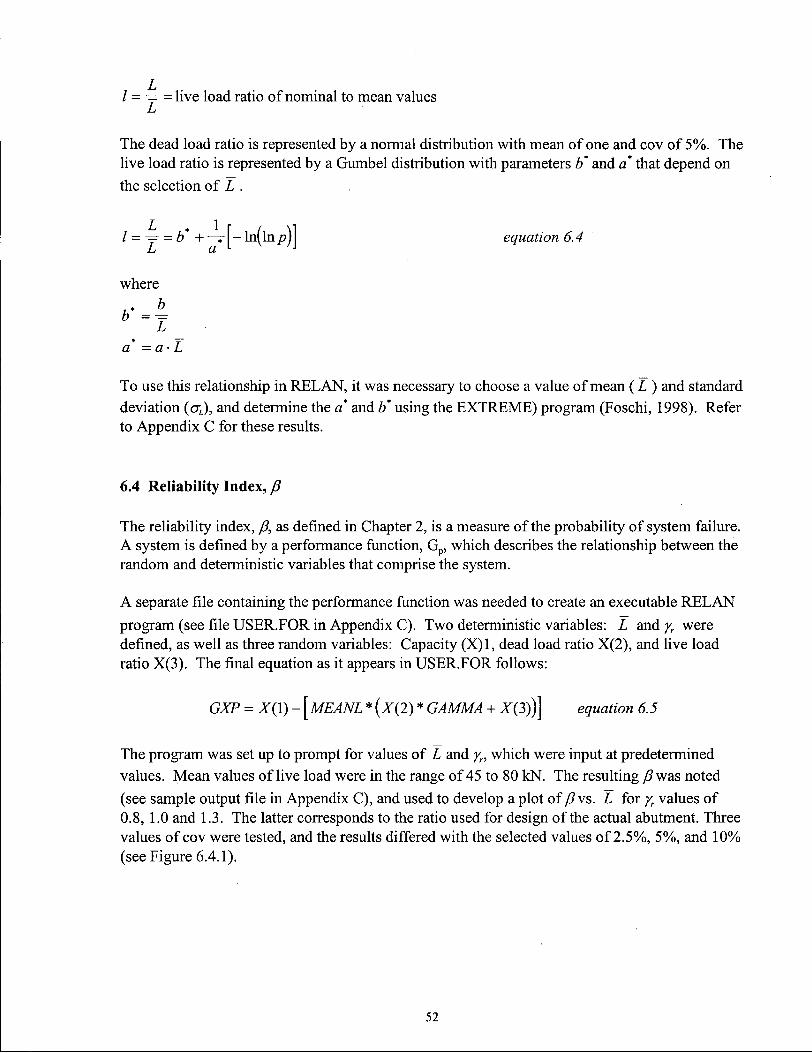
l = -== live load ratio of nominal to mean values

The dead load ratio is represented by a normal distribution with mean of one and cov of 5%. The live load ratio is represented by a Gumbel distribution with parameters b* and a that depend on the selection of L .

To use this relationship in R E L A N , it was necessary to choose a value of mean ( L ) and standard deviation (aL), and determine the a* and b* using the EXTREME) program (Foschi, 1998). Refer to Appendix C for these results.

6.4 Reliability Index, B

The reliability index, B, as defined in Chapter 2, is a measure of the probability of system failure. A system is defined by a performance function, G p , which describes the relationship between the random and deterministic variables that comprise the system.

A separate file containing the performance function was needed to create an executable R E L A N program (see file USER.FOR in Appendix C). Two deterministic variables: L and yr were defined, as well as three random variables: Capacity (X) l , dead load ratio X(2), and live load ratio X(3). The final equation as it appears in USER.FOR follows:

The program was set up to prompt for values of L and yr, which were input at predetermined values. Mean values of live load were in the range of 45 to 80 kN. The resulting /? was noted (see sample output file in Appendix C), and used to develop a plot of B vs. L for yr values of 0.8, 1.0 and 1.3. The latter corresponds to the ratio used for design of the actual abutment. Three values of cov were tested, and the results differed with the selected values of 2.5%, 5%, and 10% (see Figure 6.4.1).

equation 6.4

where

a* = a •

GXP = X ( l ) - [MEANL * (X(2) * GAMMA + X(3))] equation 6.5

52

p vs. Mean Live Load cov = 5%

55 65 75 Mean Live Load (kN)

85

Figure 6.4.1.b 6 vs. L for cov = 5%

p vs Mean Live Load cov = 10%

55 65 75 Mean Live Load (kN)

85

Figure 6.4.1.c /?vs. L for cov =10%

The live load used in the design of the abutment was 45 kN. This corresponds to the Rvalues in

Table 6.4.1. The dead load used was 57 kN, which yields a Rvalue of 1.27.

53

Table 6.4.1. Values of B for L =45 kN I cov (%)

yr 5% 10% 0.8 8.1 5.7 1.0 7.4 5.2 1.3 6.2 4.5

The value of reliability index for this abutment is higher than that considered by the Canadian Highway Bridge Design Code (CHBDC). The CHBDC uses a Rvalue of 3.5 as the basis for shallow foundation design. The results of this analysis suggest that this abutment design is more reliable than the CHBDC specifications require. Comparison of the Rvalues for the different cov values shows that the reliability index increases with a smaller standard deviation of mean live load. This is reasonable because the uncertainty is lessened when the scatter of live loads can be reduced.

The R E L A N values of B were checked by simplifying the problem, and using the the Cornell beta equation for normal variables (Cornell, 1969).

The results from the F L A C analysis were used for the capacity values: C = 148.84 kN rj c = 4.3329 kN

For demand, the live load and dead load from the MoTH design calculations were combined, and a cov of 10% was used. Thus, the values used were: D = 101.9 kN a D = 10.19 kN

Using the above values, the Cornell equation gives a value of B equal to 4.24. This value can be compared to a B value of 4.46 for cov = 10%, and yr = 1.3 from the R E L A N analysis. Comparisons of the B values for other mean live loads can be seen in Figure 6.4.2.

C-D equation 6.6

54

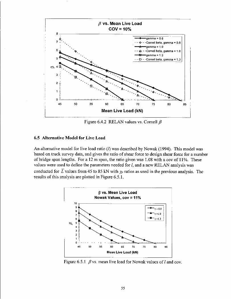
B v s . Mean L ive Load C O V = 1 0 %

• gamma = 0.8 - - -0- - -Cornell beta, gamma = 0.8

iii gamma = 1.0 - - -tc - -Cornell beta, gamma = 1.0 — B — gamma = 1.3 - - -D - -Cornell beta, gamma = 1.3

60 65 70 75

Mean Live Load (kN)

80 85

Figure 6.4.2 R E L A N values vs. Cornell B

6.5 Alternative Model for Live Load

A n alternative model for live load ratio (/) was described by Nowak (1994). This model was based on truck survey data, and gives the ratio of shear force to design shear force for a number of bridge span lengths. For a 12 m span, the ratio given was 1.08 with a cov of 11%. These values were used to define the parameters needed for /, and a new R E L A N analysis was conducted for L values from 45 to 85 kN with yr ratios as used in the previous analysis. The results of this analysis are plotted in Figure 6.5.1.

p vs. Mean Live Load Nowak Values, cov = 11%

10 T

Mean Live Load (kN)

Figure 6.5.1 B vs. mean live load for Nowak values of / and cov.

55

This model yields higher values of B at 45 kN, but the relationships have a steeper slope and tend to drop off more sharply than the Gumbel live load model.

6.6 Summary

The results of the reliability analysis indicate that the structure designed using WSD is more reliable than is necessary based on the proposed CHBDC. The partial factors for LSD were calibrated based on a reliability analysis that used a target B value of 3.5. However, the reliability analysis conducted for this particular structure predicted a B value of 4.5 when the design loads were considered. Thus, the abutment and embankment are overdesigned in terms of the proposed design methods in the draft CHBDC.

56

Chapter 7. Dynamic Analysis of No. 5 Road Overpass Abutment

The Lower Mainland of British Columbia is subject to seismic activity, and structures (including foundations) must be designed to take this into account. Most of the seismic activity in the Lower Mainland is a result of the interactions of the North American plate, the Juan de Fuca plate, the Explorer plate, and the Pacific plate. Earthquakes recorded in the Lower Mainland have been either crustal or intraplate. There has been no recorded interplate subduction earthquake, although the Juan de Fuca and Pacific plates are subducting beneath the North American plate, and earthquakes of this type may occur at or very close to any site in the Lower Mainland (Anderson et al. 1998). The frequency of the subduction earthquake is predicted to be every 300 - 500 years (Hyndman, 1995). For this reason, design spectra including the subduction earthquake wil l be brought into the next version of the N B C C . The C H B D C specifies that designs should be able to withstand a 1 in 475 year earthquake which corresponds to a Peak Ground Acceleration (PGA) for firm ground of 0.2lg in this region (Anderson et al., 1998).

Two programs were used for the dynamic analysis of the abutment soil-structure system. S H A K E (Schnabel et al., 1972) was employed first to determine the amplification of the earthquake induced accelerations. Earthquakes recorded at rigid sites were input to the stiff till layer of the delta, and propagated upwards through the soil column model. The result of this analysis (in the form of an acceleration record at the surface of the column) was taken to the dynamic F L A C model and used as the input base motion for the soil-structure system.

7.1 SHAKE Analysis

The geology of the Fraser Delta dictated that the S H A K E analysis be carried out to evaluate the effect of the deep soil layers present beneath the abutment. It is well known that the characteristics of accelerations change as they pass through soft soil. The S H A K E analysis allowed for a computation of these effects using an equivalent linear analysis.

7.1.1 Soil Column

The Fraser Delta developed after the withdrawal of the Pleistocene ice sheet (10,000 to 15,000 years ago), and consists of an uneven bedrock surface overlain by glacial till, marine clays, and silts which were lain down early in the post glacial period. These deposits were covered with deltaic forests and fluvial sands with the advancement of the delta. The sand layers vary in thickness and were eventually overlain with floodplain silts, clays, and in some areas, peat, of 3-6 m thickness. The depth of the more dense Pleistocene deposits varies from 20-30 m in eastern Richmond and adjacent to the north arm of the Fraser River to over 300 m in downtown and southern Richmond. These soils are highly variable in composition and thickness (Byrne et al., 1998).

The soil data for the S H A K E analysis were based on test hole FD94-4 provided by the Geological Survey of Canada (GSC). The test hole went to a depth of 300 m and provided information on soil type, plasticity index, and shear wave velocity. Ti l l was encountered at a

57

depth of approximately 240 m. The soil profile can be seen in Figure 7.1.1 and the shear wave velocities are plotted in Figure 7.1.2.

silty sand (organic clay layer embedded) V s = 125 m/s f= 19 kN/m3 Depth 6 m

V s = 125 m/s silty sand

7= 19.5 kN/m 3 Depth 14 m

V s = 150 m/s silty sand

7= 19.5 kN/m 3 Depth 20 m

V s = 170 m/s silty sand

y= 19.5 kN/m 3 Depth 24 m

Vs = 200 m/s sandy si l t

y= 19.0 kN/m 3 Depth 30 m

Vs = 225 m/s sandy si l t

7 = 19.0 kN/m 3 Depth 32 m

V s = 225 m/s

silty sand y= 19.5 kN/m 3 Depth 36 m

V s = 250 m/s silty sand

7 = 19.5 kN/m 3 Depth 38 m

V s = 250 m/s

sandy si l t 7 = 19.0 kN/m 3 Depth 45 m

V s = 250 m/s silty sand

7= 19.5 kN/m 3 Depth 47 m

V s = 300 m/s

silty sand 7= 19.5 kN/m 3 Depth 60 m

V s = 300 m/s clay and si l t

7 = 20.5 kN/m 3 Depth 70 m

V s = 325 m/s

clay and si l t 7=20.5 kN/m 3 Depth 80 m

V s = 350 m/s clay and si l t 7=20.5 kN/m 3 Depth 90 m

V s = 375 m/s clay and si l t

7 = 20.5 kN/m 3 Depth 140 m

V s = 400 m/s

clay and si l t 7=20.5 kN/m 3 Depth 150 m

V s = 450 m/s

clay and si l t y= 20.5 kN/m 3 Depth 190 m

Vs = 500 m/s clay and si l t

y= 20.5 kN/m 3 Depth 210 m

V s = 500 m/s clay and si l t

7=21 kN/m 3 Depth 220 m

Vs = 600 m/s

clay and si l t 7= 21 kN/m 3 Depth 230 m

Vs = 700 m/s clay and si l t

7= 21 kN/m 3 Depth 240 m

Figure 7.1.1 Soil Profile used in S H A K E column

58

50

- g - 100

<D 150

200

250

Shear Wave Velocity with Depth of Soil Column

\

0 200 400 600 800

Shear Wave Velocity - Vs (rrVs)

Figure 7.1.2 Shear Wave Velocity as recorded by GSC.

ShakEdit (Ordonez, 1998) requires only density and shear wave velocities to be input, and calculates the shear modulus based on equation 2.3.1. Idriss' (1990) values of damping ratio and shear modulus reduction for sand and clay were used (Figures 7.1.3 and 7.1.4). These particular values as functions of shear strain were selected based on curves published by Seed and Idriss (1970) and by Sun et al. (1988). Idriss showed that these values gave a good correlation between recorded data on soft-soil sites and S H A K E soil columns of the sites when compared to rigid base input records. He also concluded that the peak horizontal accelerations on soft soil sites during the Loma Prieta earthquake were about 1.5 to 3 times those obtained at nearby rock sites, and that equivalent linear response analyses provided a reasonably accurate estimation of peak horizontal accelerations in the San Francisco Bay area during the 1989 Loma Prieta earthquake.

59

Damping Ratio vs. Strain Sand and Clay

(Q at c 'a. E « Q

25

20

15 -t

10

0 * 0.0001 0.001 0.01

P e r c e n t S t ra in

Figure 7.1.3 Damping Curve for Sand and Clay from Idriss (1990)

Modulus Reduction after Idriss (1990)

1.2

0.8 X ID

(3 0.6

0 0.4

0.2

zzzizEBilii

: - » - G / G m a x c lay

— • — G / G m a x sand

0

0.0001 0.001 0.01 0.1

P e r c e n t S t ra in

Figure 7.1.4 Modulus Reduction Values from Idriss (1990)

The maximum number of layers allowed in S H A K E is 50, and this particular column was divided into 43 layers. This large number of layers was used in order to better model the variation in shear modulus and damping with strain throughout the depth of the soil column. Having a large number of layers also allowed for information at specific depths, as output is generated only at the top of each layer.

The shear wave velocity at the base was set to 6500 fps which assumed that the bedrock is sedimentary rock or partially consolidated sediment/till (personal communication, Singh, 1999). The densities were varied based on silt content, and depth throughout the column. The

60

surrounding soil has been densified to avoid liquefaction, and this is accounted for with slightly higher values of density in the S H A K E column.

7.1.2 Input Earthquakes

Prior to the main analysis with the full-length column, a number of acceleration records were tested in a variety of soil columns to investigate the difference in response and to get a feel for the S H A K E analysis. A summary of these test runs can be seen in Appendix E.

Six earthquakes were chosen for the dynamic analysis with the soil column presented earlier (Figure 7.1.1). One of the earthquakes (caltechb) is a natural record that was scaled to a P G A of 0.2 lg . The remaining five earthquakes were fit to the Vancouver Uniform Hazard Response Spectrum (Van UHRS '99, Figure 7.1.5) and scaled to 0.21g. The Van UHRS 1999 has been developed as a design guide when selecting or modifying earthquakes to use in dynamic analyses. This type of design spectrum has an equal probability of being exceeded at all periods of vibration (Kramer, 1996). The earthquakes used in analysis are tabulated below (Table 7.1.1) with direction, source, and date of occurrence.

0.6

O) 0.5

ti U) 0.4 TJ a 0.3 E •g 0.2

0

0 0.2 0.4 0.6 0.8 1 1.2

Per iod , sec

Figure 7.1.5 Vancouver Uniform Hazard Response Spectrum, 1999

Figure 7.1.6 shows the input accelerations (in g) for the Caltechb and 316 earthquake records, and Figure 7.1.7 shows the corresponding response spectra for the earthquakes. The 316 record is the Caltechb record that has been modified to fit the Vancouver UHRS 1999. Note that the records look significantly different, although both are scaled to 0.2lg. The time histories for the remaining earthquakes can be viewed in Appendix E. It is interesting to observe the similarities between the modified records, and their differences from the natural record, especially in the response spectra. A l l earthquake modifications were performed by Dr. Don Anderson of the University of British Columbia using the program S Y N T H (1985).

61

Table 7.1.1 Earthquake acceleration records used in dynamic analysis Record Nickname Date Direction Type

Lorna Prieta lpns 1989 NS Modified to Van UHRS '99 Loma Prieta lpew 1989 EW Modified to Van UHRS '99

Miyagiken-Oku miew 1978 EW Modified to Van UHRS '99 San Fernando 316 1971 EW Modified to Van UHRS '99 San Fernando 317 1971 NS Modified to Van UHRS '99 San Fernando caltechb 1971 EW Natural record - scaled only

0.3

-0.3 -f—• ' i ' i ' ' i i i i ' i i i i i | i , i , | , , , , |

0 5 10 15 20 25 30 35 40

Time (seconds)

Figure 7.1.6.a Input Time History - caltechb

0.3

-0.2 4

-0.3 -I • • 1 • - n - ' 1 • - - r - • 1 • - - r - ' 1 0 5 10 15 20 25 30 35 40

Time (seconds)

Figure 7.1.6.b Input Time History - 316

62

D) 0.7

0.01 0.1 1 10

P e r i o d (s)

Figure 7.1.7.b Input Response Spectra for all Earthquakes

7.1.3 Resulting Accelerations and Amplifications

The layer of interest in the S H A K E column was layer 2, at a depth of 2.5 m. The abutment structure is built on the ground surface, with only a 2 m excavation of the natural soil. The response at this layer was investigated in terms of the resulting acceleration history, and the response spectrum. The time histories at the surface (Figure 7.1.8) are plotted for caltechb and 316 for comparison with the input histories (Figure 7.1.6). The response spectra for the surface layer, and the ratio of response spectra of surface to base are also shown in Figures 7.1.9, and 7.1.10. Note that there is no amplification at the PGA, except for the natural caltechb record. The S H A K E analysis showed that the first natural period lies around 2.6 seconds, with the sequentially following periods being 1.61, 0.86, and 0.63. In the ratio plots, it can be seen that there is amplification in these regions, as the amplification ratio becomes greater than one at a

6 3

period of around 0.4 seconds. This is thought to be a property of the very long soil column, which has an inherently high natural period.

Figure 7.1.8.a Time History at Layer 2 of S H A K E Column - Caltechb

3 c o l_ 0) ~o u u <

0.2

0.1

0

-0.1

-0.2

•4 # h 1 1 1 1 1 ' 1 1 ' i ' ' ' 1 1 ' ' ' ' i 1 1 ' 1 1 1 1 ' 1

0 10 20 30 40

Time (s)

50 60

Figure 7.1.8.b Time History at Layer 2 of S H A K E Column - 316

64

0.7

0.01 0.1 1 10

P e r i o d (s)

Figure 7.1.9.a Surface Response Spectra- Caltechb and 316

0.7

0.01 0.1 1 10

Period (s)

Figure 7.1.9.b Surface Response Spectra- all Earthquakes

65

10

Period (s)

Figure 7.1.10.a Ratio of Surface to Base Spectra - Caltechb and 316

c o

Period (s)

Figure 7.1.10.b Ratio of Surface to Base Spectra - all Earthquakes

7.2 Comparison with F L A C Column.

A one-element wide grid was developed in F L A C to check the results of S H A K E and to determine appropriate values of damping and modulus reduction factors. The two main parameters checked were peak ground acceleration (input and resulting surface values) and the maximum shear stresses.

Maximum strains with depth were taken from the S H A K E results, and the strains were then used to find the corresponding damping and modulus reduction values. These values were used as initial inputs for the F L A C column model, and were refined by a trial and error process to obtain reasonable correlation of acceleration and shear stress values between the S H A K E and F L A C columns (Table 7.2.1).

Table 7.2.1.a Comparisons between S H A K E and F L A C columns caltechb 316 . 317

F L A C S H A K E F L A C S H A K E F L A C S H A K E Peak Ground Accelerations (g'

input 0.21 0.21 0.21 0.21 0.21 0.21 surface 0.21 0.22 0.16 0.17 0.16 0.17.

Shear Stresses (kPa^ base 130 • 134 141 158 198 158 , 200 m 127 • 124 119 148 171 148 150 m 104 105 95 120 150 120 50 m 78 72 59 62 • 74 86 20 m 43 ' 29 32 34 .34 34

Table 7.2.1.b Comparisons between S H A K E and F L A C columns lpns lpew miew

F L A C S H A K E F L A C S H A K E F L A C S H A K E Peak Ground Accelerations (g

input 0.21 0.21 0.21 0.21 0.21 0.21 surface 0.14 0.14 0.13 0.13 0.14 0.15

Shear Stresses (kPa base 142 140 164 141 227 187 200 m 123 134 147 124 194 182 150 m 100 115 106' 105 153 148 50 m 51 64 55 62 61 72 20 m 25 34 31 38 33 41

Note that when the accelerations decreased in the S H A K E column, they also decreased in the F L A C column. This helps to give confidence that the resulting deamplification of the PGA may be valid, and is a consequence of the soil column itself.

Some earthquakes gave closer matches between the two programs. The resulting damping ratios and modulus reduction values fall within a fairly close range. Table 7.2.2 gives the values that were used in the final F L A C dynamic model for each earthquake.

67

Table 7.2.2 Values of damping and G / G m a x used in F L A C model for each earthquake Central frequency

(Hz) Percent of Critical

Damping G/Gmax

caltechb 2 8% 0.18 316 2 10% 0.18 317 2 11% 0.20 lpns 2 11% 0.18 Ipew 2 12% 0.12 miew 2 12% 0.12

7.3 Questionnaire

A questionnaire was developed in order to gain "expert judgement" on the soil properties of Fraser River Sand. The questions involved estimating mean values and ranges of values for properties such as friction angle, unit weight, saturation, and (Ni)6o- Five questionnaires were sent out to five different geotechnical engineering companies in the Lower Mainland, and three responses were received from two companies. A sample questionnaire can be found in Appendix G, along with the responses obtained. The results are summarised in Table 7.3.1.

Table 7.3.1 Questionnaire Results Friction Angle Unit Weight (Ni)6o expected when 20

(degrees) (kN/m3) is specified Respondent Mean a Mean a Mean a

1 33.3 9.0 19.1 2.2 22.6 2.5 2 38.3 4.3 15.0 7.5 23.5 13.2 3 33.0 5.0 18.0 0.5 16.6 18.1

The values from Respondent 1 were used as the base values for the analysis, but a sensitivity analysis was carried out which included the ranges favoured and indicated by the two other respondents. The results from the saturation question were very different from respondent to respondent, and so values of mean and standard deviation could not be reasonably calculated.

7.4 FLAC Model for Dynamic Analysis

The F L A C model used for the dynamic analysis was a modification of the static model. The depth of the model was extended by 2 m and the grid was widened (Figure 7.4.1). Free field boundaries were applied to the right and left boundaries of the model to simulate an infinite model and avoid reflection effects from the earthquake.

The acceleration records were applied at the base of the model, and a correction was made during stepping to account for the lack of baseline correction of the input accelerations. The input file, including FISH functions, can be viewed in Appendix F.

68

JOB TITLE :

FLAC (Version 3.40)

LEGEND

24-Apr-99 0:02 step 1012000

-1.284E+00 <x< 2.439E+01 -7.839E+00 <y< 1.784E+01

Grid plot I I I I I I 0 5E 0

Beam plot

MoTH Geotechnical British Columbia

Figure 7.4.1 F L A C Mesh for Dynamic Analysis.

The values of shear modulus reduction factor and damping values from the S H A K E - F L A C column analysis were also incorporated into the model, with the values changing for each earthquake. The plastic soil model used was the Mohr-Coulomb model (as it was for the static analysis), and the necessary soil properties were input according to the type of results required. An analysis to determine the expected value of displacement was carried out, along with a sensitivity analysis to ascertain which variables have the greatest effect on the results.

7.5 Expected Value of Displacement

Knowledge of the expected level of displacement that would occur during an earthquake event was desired. To achieve this objective, the F L A C model was run with a flight of five acceleration records. The records used were the resulting accelerations at layer 2 from the S H A K E analyses with corresponding damping and shear modulus reduction factors as described in section 7.2. Only those earthquakes modified to fit the Van UHRS '99 were used in this section of the analysis.

In order to determine an expected value, probabilities were required for various combinations of soil properties. Density was assumed to be relatively constant (as it is the best known property of Fraser River Sand), and set to a value of 19 kN/m 3 . The friction angle and (N\)6o were varied for each run, with the combinations as shown in Table 7.5.1.

69

Table 7.5.1 Combinations of Friction Angle and (Ni)6o Combination Friction Angle (N.)60 Probability Normalised

Probability 1 33 18 0.0375 0.0385 2 33 23 0.6750 0.6923 3 33 28 0.0375 0.0385 4 28 23 0.0900 0.0923 5 38 23 0.1350 0.1385

The probabilities for the occurrence of each soil property, P[$ and P[(Ni) 6 0], were obtained from the responses to the soils questionnaire described in Section 7.3. In order to determine probabilities for joint occurrence of these properties, it had to be assumed that they were independent, and non-correlated. In doing so, the probability of the intersection of the two events was simply the product of the probabilities of each event.

P[(/> n (/V,) 6 0] = P{<j>) • P[(N{ ) 6 0] equation 7.5.1

These combinations are not completely mutually exclusive and exhaustive (i.e. the probabilities add up to 0.975 as opposed to 1.0), but they do include the most probable combinations of occurrence. The resulting probabilities were normalised so as to model a mutually exclusive and exhaustive system. Another issue is that the properties are not independent of each other. This can be resolved by considering the manner in which the probabilities were initially obtained. Because the probabilities are based on expert judgement, the correlation is inherent in the selection of values. The experts give more weight to those possibilities that they would expect to occur. In any case, the higher probabilities are related to the combinations that are thought to have the highest occurrence probability. For example, the combination involving the mean values of friction and (Ni)6o has the highest probability associated with it, as would be expected.

Each combination was excited by each earthquake, with 25 F L A C runs being done in all for this portion of the analysis. The deformed mesh and displacement vectors are shown in Figure 7.5.1 and 7.5.2. The resulting displacements were multiplied by the probability of that particular combination occurring and summed to determine the expected value of displacement for each combination. Values for each earthquake were averaged with the others to obtain the average expected displacement. Overall surface plots of the probability and expected displacement values versus (Nj)6o and friction angle can be viewed in Figure 7.5.3. The surface plots were developed using the Kriging geostatistical gridding method in the program SURFER (1994). The probability plot sees a high point in near the mean values of (Ni)6o and friction angle, but when the results of the F L A C analyses are multiplied by the probability of the specified combination occurring, it can been seen that the high points shift toward lower values of friction angle, as would be expected (Figure 7.5.3 b and c).

70

JOB TfTLE :

FLAC (Version 3.40)

LEGEND

24-Apr-99 0:02 step 1012000 -1.284E+00<x< 2.439E+01 -7.839E+00 <y< 1.784E+01

Exaggerated Grid Distortion Magnification = 1.734E+01 MaxDisp= 1.058E-01

MoTH Geotechnical British Columbia

Figure 7.5.1 Deformed F L A C Mesh after Earthquake Applied.

JOB TITLE :

FLAC (Version 3.40)

LEGEND

24-Apr-99 0:02 step 1012000 -1.284E+00 <x< 2.439E+01 -7.839E+00 <y< 1.784E+01

Displacement vectors Max Vector = 1.058E-01

0 2E -1

MoTH Geotechnical British Columbia

Figure 7.5.2 Displacement Vectors after Earthquake Applied.

71

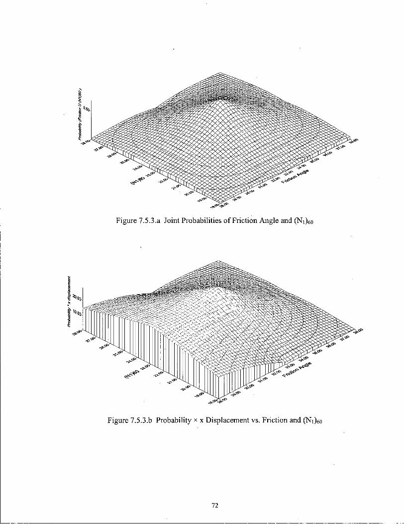
Figure 7.5.3.a Joint Probabilities of Friction Angle and (N\)eo

72

Figure 7.5.3.C Probability x y Displacement vs. Friction and (Ni)6o

The resulting expected value of displacement at the seat of the abutment is 61 mm horizontal and 36 mm vertical for this particular structure subjected to an earthquake that fits the Vancouver UHRS.

7.6 Sensitivity Analysis in F L A C

One main issue when dealing with soil models is the variability of the soil properties. In the static case, this was investigated using the rdev function in F L A C which scattered the properties throughout the grid according to a specified normal distribution for each property. For the dynamic analysis, a different technique was used. One earthquake was selected, and sensitivity analyses were run to determine the properties that most affect the results. The values for the analysis were based on the results of the questionnaire described in section 7.3. The natural caltechb record was scaled to 0.2lg and run through a S H A K E column to determine soil amplification effects before it was applied to the F L A C model for all sensitivity analyses. Sensitivity was investigated for friction angle, density, and (Ni)6o- Correlations were also developed (Campanella et al., 1995) between these properties for use in a randomisation run. The value of ( N i ) 6 o was set to a normal distribution and scattered through the mesh using a FISH function, and the correlated values of friction angle and density were set to match the scattered values.

7.6.1 Friction Angle

Four values of friction angle were chosen for the sensitivity analysis. The values were 30, 33, 36, and 39 degrees. A friction angle of 33 corresponds to the mean values given by Respondents 1 and 3. Respondent 2 chose 38 degrees, which is closely represented by the analysis using 39 degrees. The resulting displacements for each run can be seen in Table 7.6.1 (x and y being

73

horizontal and vertical displacement, respectively). These displacements were normalised to the expected value obtained from the multi-earthquake run of section 7.5. and plotted in Figure 7.6.1. The resulting displacements vary widely with choice of friction angle. Note that there is a significant difference in predicted displacement (approximately 2 times) for a friction angle of 39° as opposed to 33°. This indicates differences that may be expected in analyses conducted by various engineers. Respondents 1 and 3 would predict much larger displacements than Respondent 2, and the resulting designs would be duly affected.

Table 7.6.1 Results of sensitivity analysis on friction angle. Friction Angle x displacement (mm) y displacement (mm)

30 102.8 59.69 33 48.76 29.05 36 33.07 20.16 39 20.66 15.77

3.00

jB 2.50 o o a. x UJ

§ 2.00 E 8 1.50

0) OS

E a 8 1.00

$ 0.50

0.00

30

—•— ydisp

— x d i s p

—•— ydisp

— x d i s p

i i I I i i

32 34 36 38

Fr i c t i on A n g l e , <f>

Figure 7.6.1 Sensitivity Analysis on Friction Angle

A trial run was done for this analysis using an earthquake record that had not been sent through the S H A K E column. It is interesting to note that the resulting displacements were lower for all friction angles. Thus, eliminating the effect of the deep soil layer as modelled in S H A K E would have resulted in lower estimates of displacement.

7.6.2 Unit Weight

The unit weight values chosen for the sensitivity analysis were within a narrow range, as a result of the small variations predicted by the respondents. The unit weights used were 17, 18 , 19 and 20 kN/m 3 . The results are tabulated and charted as for friction angle, and can be viewed in Table

74

7.6.2 and Figure 7.6.2. Note that the change in resulting displacements for different unit weights is relatively insignificant compared to the sensitivity analysis on the friction angle.

Table 7.6.2 Results of sensitivity analysis on unit weight Unit Weight (kN/m J) x displacement (mm) y displacement (mm)

17 50.85 34.15 18 50.86 31.82 19 47.72 27.62 20 48.25 26.59

3 O O a. x LU C

E OJ o re a W

Q

1 00 j

0 95 ,| ~0 90 --c f 0 85 1 0) o O

80 -re

80 -£o 75 --5 0 70

0 65 -0 60 -

17 17.5 18 18.5 19 19.5 20

Uni t W e i g h t (kN/m 3 )

Figure 7.6.2 Sensitivity Analysis on Unit Weight

7.6.3 (N i ) 60

Although (Ni)6o is not itself a F L A C input parameter, it is needed to define the stiffness and strength of the soil model in terms of shear and bulk modulus (equation 2.3.2). The sensitivity on (N 1)60 was checked in two different ways. The first followed the same method as for the friction angle and unit weight. Four values were chosen, those being 18, 20, 23, and 28. Two respondents chose values near 23, while the third was slightly pessimistic, and chose a value of only 17 when the specified (N\)eo was to be 20. To represent this belief, a value below 20 was chosen for the sensitivity analysis. The results of these runs can be seen in Table 7.6.3 and Figure 7.6.3.

75

Table 7.6.3 Results of sensitivity analysis on (Ni)6o

(Ni)60 x displacement (mm) y displacement (mm) 18 23.28 16.87 20 20.31 15.71 23 16.42 14.46 28 13.31 13.35

Figure 7.6.3 Sensitivity Analysis on (Ni)6o

The second half of the analysis on (Ni)6o involved the use of the rdev function in F L A C . Correlations were developed between (Ni)6o, unit weight, and friction angle using the relationships compiled by Campanella et al. (1995). Values of em a x, emj n, G s , and D 5n from previous soil testing on Fraser River Sand were used (Vaid and Sivathalayan, 1996). The values used were 0.96, 0.60, 2.71, and 0.3 mm, respectively, and facilitated the determination of relative density (D r) for use in the correlation charts. Table 7.6.4 shows the discrete correlations. Note that the values of friction angle and unit weight do not change much with a 10 count difference in (Ni)eo.

Table 7.6.4 Correlations between SPT, friction angle, and unit wei; N (N,)6o q c (bars) Dr (%) d> Y 25 18 125 60 38 18.7 28 20 140 67 39 18.8 33 23 165 73 40 19.0 40 28 200 80 41 19.1

ght

A FISH function was used to generate a random normal distribution of (Ni)6o throughout the mesh, with a mean of 22.5 and a standard deviation of 2.5, after the predictions of Respondent 1. The results were very interesting in this case, because with the correlations in place, the resulting displacements were very low - much lower than any of the results from the sensitivity analysis.

76

This is due to the fact that the SPT correlations gave very high values of friction angle. As noted in the sensitivity analysis for friction angle, the displacement decreases rapidly with an increase in friction.

Figure 7.6.4 Results of Random (JNJ)6O Correlated to Friction and Unit Weight

7.7 Summary

In this situation, the underlying soil has been densified and the site has been engineered so as to avoid any liquefaction problems. Thus, large displacements are not expected, even when the design earthquake is experienced. As it stands, the only concern is for settlement due to shaking and/or excessive loading. The results of the analysis indicate a level of displacement that would not signify an exceedance of serviceability limit states, much less an ultimate limit state. The largest vertical displacement determined in the sensitivity analysis was 103 mm when the friction angle was 30° (i.e. at its lowest value). According to engineers at MoTH (Gillespie and Szto, 1999), the serviceability after an earthquake only becomes an issue if the settlements are in the order of 300 mm (3 times the worst expected case). Thus, the expected values of displacement (61 mm horizontal, and 36 mm vertical) are of no concern in this particular case. This may be another indication that the abutment is more reliable than is actually necessary.

The soil parameter that was found to be the most important in the course of running the sensitivity analysis was the friction angle. A change in friction angle resulted in the greatest changes in displacements. In addition, from the questionnaire results, it appears that engineers are more confident in predicting the unit weight of this particular soil than they are with predicting friction angle, or (N])6o- This uncertainty in the determination of parameters must be considered along with the wide range of results due to the choice of different values of the parameters when designing foundation structures.

77

Chapter 8. Conclusions and Recommendations

A great deal of information has been presented on LSD and WSD along with numerous models, analyses, and design calculations. The initial purpose of this work was to compare the design differences between WSD and LSD. LSD and WSD can be compared based on the results of the analyses, as well as on the efficiency in design methods. The analyses performed include a direct comparison of WSD and LSD methods, a reliability analysis, a dynamic sensitivity analysis, and an expected displacement analysis based on a design response spectrum. In terms of efficiency, WSD and LSD can be compared based on design methods and economy of the resulting design.

8.1 Comparison Based on Results of Analyses.

The first part of the comparison involves the LSD calculations performed on the existing No. 5 Road overpass abutment according to the CHBDC. A LSD ratio was calculated based on the basic concept of FS. In this way, the LSD ratio was used to compare the WSD and LSD methods, as explained in Chapter 5. The LSD calculations resulted in high values of factored resistances, which led to high LSD ratios. In fact, these values were higher than the global FS that were accepted for the original WSD. Assuming the LSD method is reliable (based on its calibration with WSD and reliability analysis), one can conclude that the abutment structure designed using WSD is less efficient and more conservative than required by C H B D C 1998.

A second method of comparison is the combined F L A C and R E L A N analysis that was used to determine a reliability index for this particular structure. The existing abutment was modelled in F L A C and a reliability analysis was conducted to determine the B value for the abutment and embankment. This type of analysis would not generally be performed for such a situation, but in this case it allows a direct comparison of the objectives and results of the designs. LSD, as presented by the CHBDC, is based on a reliability index of 3.5. The results of this particular reliability analysis gave a reliability index of 4.5 for the design loads. This indicates that the existing structure is more reliable than is required by the CHBDC.

The expected displacement analysis offers another mode of comparison. This method addresses the dynamic problem resulting from the location of the structure within a region of significant seismicity. The expected displacement was determined based on a number of F L A C runs using a flight of earthquakes and combinations of soil properties. This analysis showed the combinations that were likely to yield the greatest overall response (i.e. displacement). Probabilities on the various combinations were derived from "expert judgement" as a result of a questionnaire sent out to experienced geotechnical engineers in the Lower Mainland. The resulting expected displacements for the existing structure designed using WSD were very low, and, as such, are not high enough to cause a serviceability concern, much less failure. The insignificant displacements in the earthquake problem are another indication that the initial structure may have been overdesigned as a result of using WSD.

78

8.2 Comparison Based on Efficiency

When one considers the amount of time it takes to perform the design calculations, WSD appears efficient since there is no confusion as to what calculations are necessary. This is simply due to familiarity with the method. However, LSD requires the same basic calculations and will become as efficient a method of design and analysis with time and regular usage. LSD will provide a "bridge" between geotechnical engineers and structural engineers because of the terminology and the resulting values of resistance. In addition, using partial factors may help the engineer to seriously consider what forces are acting on the foundations and how these forces affect the behaviour of the structure.

If efficiency in design (or economy) was considered, one would have to consider that the LSD analysis of the existing structure showed a large margin of safety in ULS and SLS. This indicates that the structure could be downsized and still meet the LSD criteria. A smaller structure would have a lower resistance (in bearing ULS and SLS), and would also be more economical by requiring less material. However, one of the main factors in abutment design is simply the geometry of the structure including the bridge, the embankment, and the connections. If the design is based solely on these factors, then it may not be possible to reduce the size and increase the efficiency of the structure. Another consideration is that the size difference between a WSD and a more efficient LSD design may not be significant enough to justify a change in design. The engineer may choose to stay with the marginally safer WSD instead of saving a small percentage of the construction cost.

8.3 Recommendations for Further Work

It is possible that structures designed using LSD may still be excessively safe when compared to the results of a finite difference analysis. However, this remains to be seen, and it would be beneficial to follow-up this study by running the same kind of reliability analysis on a structure designed using the new code. It would be interesting to see what kind of reliability index emerges from the procedure followed in this thesis, and what types of expected displacements would be calculated.

79

References

AASHTO. 1983. ATC-6 Seismic Design Guidelines for Highway Bridges. American Association of State Highway and Transportation Officials. Washington, D.C.

AASHTO. 1989. Guide Specifications for Seismic Design of Highway Bridges. American Association of State Highway and Transportation Officials. Washington, D.C.

Allen, D.E. 1974. Limit States Design - A Probabilistic Study. Canadian Journal of Civi l Engineering, Vol . 2. pp. 36-49.

Allen, D.E., 1982. CBD-221. Limit States Design, Canadian Building Digest. January 1982.

Anderson D.L., Byrne P.M. , Nathan, N.D. 1998. Seismic Hazard Study - Lower Mainland Soft Soil Sites. Vancouver BC. prepared for Ministry of Transportation and Highways, Province of British Columbia.

Applied Technology Council, 1983. Seismic Design Guidelines for Highway Bridges ATC-6.

Applied Technology Council, 1996. Improved Seismic Design Criteria for California Bridges: Provisional Recommendations. ATC-32.

Applied Technology Council, 1997. Seismic design criteria for bridges and other highway structures: current and future. ATC-18. Chapter 6. U.S. and Foreign Requirements for Abutments and Retaining Walls.

Application of Centrifuge Modelling to Geotechnical Design. Proceedings of a Symposium on the Application of Centrifuge Modelling to Geotechnical Design. Manchester. 16-18 April 1984. Edited by W.H. Craig. A . A . Balkema, Rotterdam, Boston.

Becker, D.E. 1996 Eighteenth Canadian Geotechnical Colloquium: Limit States Design for Foundations. Part I. A n overview of the foundation design process. Canadian Geotechnical Journal. Vol . 33, No. 6, pp. 956-983.

Becker, D.E. 1996 Eighteenth Canadian Geotechnical Colloquium: Limit States Design for Foundations. Part II. Development for the National Building Code of Canada. Canadian Geotechnical Journal. Vol . 33, No. 6, pp. 984-1007.

Becker, D.E. 1998. Workshop on Limit States Design for Foundations Draft Canadian Highway Bridge Design Code. Canadian Geotechnical Society 1998 Cross-Canada Lecture Tour, Canadian Geotechnical Society. British Columbia Ministry of

80

Transportation and Highways - Geotechnical and Materials Branch, Victoria, B C November 27.

Becker, D.E., Allen, D.E., Ho, K.S., and Law, K.T. 1993. Development of Limit States Design for Foundations in the National Building Code of Canada. International Symposium on Geotechnical Limit States Design (ISLSD), Copenhagen, 26-28 May 1993. pp 479-489.

Benjamin, J.R. and Cornell, C A . 1970. Probability, Statistics, and Decision for Civ i l Engineers. McGraw-Hill Book Company.

th

Bowles J.E. 1996. Foundation Analysis and Design, 5 Edition, McGraw-Hill Publishing Company, N . Y .

Brinch Hansen, J. 1953. Earth pressure calculation. The Danish Geotechnical Press, Copenhagen.

Brinch Hansen, J. 1956. Limit state and safety factors in soil mechanics. [In Danish with an English summary.] Danish Geotechnical Institute, Copenhagen, Bulletin N o . l .

Byrne P .M. , Anderson D.L., Naesgaard E., and Atigh E. 1998. Seismic Behaviour of Box Culverts in Richmond. Report to the City of Richmond.

Byrne P .M. , Cheung H. , and Yan L. 1987. Soil Parameters for deformation analysis of sand masses. Canadian Geotechnical Journal, Vol . 24, pp. 366-376.

Campanella, R.G., and students. 1995. Interpretation of Piezocone Test Data for Geotechnical Design. Soil Mechanics series 157 and 158, In-Situ Soil Testing Research Group, Department of Civi l Engineering, University of British Columbia. September.

Canadian Standards Association. 1981. Guidelines for the Development of Limit States Design. C S A Special Publication S408-1981, Rexdale, ON.

Canadian Standards Association. 1978. Design of Highway Bridges - CSA Standard CAN3-S6-M78.

Canadian Standards Association. 1988. Design of Highway Bridges - CAN/CSA-S6-88.

Canadian Standards Association. 1997. Canadian Highway Bridge Design Code - Draft May 1997.

Canadian Standards Association. 1997. Canadian Highway Bridge Design Code - Draft. Commentary, Section 6. November, 1994.

Canadian Geotechnical Society. 1992. Canadian Foundation Engineering Manual, 3 r d

Edition. Canadian Geotechnical Society, Technical Committee on Foundations, 512 p.

81

Coetzee M.S., Hart R.D., Varona P.M. , and Cundall P.H. 1998. F L A C Basics: A n introduction to F L A C and a guide to its practical application in geotechnical engineering. 2 n d Revised Edition. Itasca Consulting Group, Inc. 708 South Third St, Minneapolis, Minnesota 55415 USA.

Cornell, C.A. 1969. A reliability based code format. Journal of ACI , 1969:66(13).

Craig, W.H. 1984. Centrifuge modelling for site-specific prototypes. Proceedings of a Symposium on the Application of Centrifuge Modelling to Geotechnical Design. Manchester. 16-18 April 1984. Edited by W.H. Craig. A . A . Balkema, Rotterdam, Boston, pp. 485-501.

Craig, W.H. 1995. Geotechnical centrifuges: past, present and future. Geotechnical Centrifuge Technology. Edited by R.N. Taylor, Blackie Academic and Professional, Glasglow. pp. 1-18

Dallimore, S.R., Edwardson, K . A . , Hunter, J.A., Clague, J.J. and Luternauer, J.L. 1994. Composite Geotechnical Logs for two deep boreholes in the Fraser River delta, British Columbia. Geological Survey of Canada Open File 3018.

Foschi, R.O., and Sexsmith, R.G. 1998. Class notes for CIVL 518. Department of Civi l Engineering, University of British Columbia.

Foschi, R.O. 1998. Personal communication.

Foschi, R O . 1998. Unpublished computer programs: DATAFIT, E X T R E M E , PLOT, R E L A N v2.0. Department of Civil Engineering, University of British Columbia.

Fraser, D. 1985. Foundation Report - Richmond E-W Freeway No. 5 Road Overpass, Ministry of Transportation and Highways, Geotechnical and Materials Branch, Victoria, B C , October.

Gemperline, M.C . and Ko, H.Y. 1984. Centrifugal model tests for ultimate bearing capacity of footings on steep slopes in cohesionless soils. Proceedings of a Symposium on the Application of Centrifuge Modelling to Geotechnical Design. Manchester. 16-18 April 1984. Edited by W.H. Craig. A . A . Balkema, Rotterdam, Boston, pp. 203-221

Gillespie, D. and Szto, B . 1999. Personal communication. Ministry of Transportation and Highways of British Columbia.

Green, R. 1993. LSD Code for Bridge Foundations. International Symposium on Geotechnical Limit States Design (ISLSD), Copenhagen, 26-28 May 1993. pp.459 - 468.

Hardin, B.O., and Dmevich, V.P. 1972. Shear Modulus and Damping in Soils: Design Equations and Curves. Journal of Soil Mechanics and Foundations Division, A S C E , Vol . 98, No SM7, July. pp. 667-692.

82

Hyndman, R.D. 1995. Giant Earthquakes along the West Coast of North America. Pacific Geoscience Centre of the Geological Survey of Canada.

Idriss I.M., and Sun, J.I. 1992. User's Manual for SHAKE91: A Computer Program for Conducting Equivalent Linear Seismic Response Analyses of Horizontally Layered Soil Deposits. Program Modification based on the Original S H A K E program published in December 1972 by Schnabel, Lysmer, and Seed. Center for Geotechnical Modelling, Department of Civil & Environmental Engineering, University of California, Davis, California, November.

Idriss I.M., 1990. Response of Soft Soil Sites During Earthquakes. Proceedings of the H. Bolton Seed Memorial Symposium, Vol . 2. pp. 273-289.

Ishihara K. , 1982. Evaluation of soil properties for use in earthquake response analysis. International Symposium on Numerical Models in Geomechanics. Zurich. September 1982.

Itasca Consulting Group, Inc. 1998. F L A C version 3.40. Minneapolis, Minnesota.

Itasca Consulting Group, Inc. 1998. F L A C online manual. Minneapolis, Minnesota.

Kramer, S.L., 1996. Geotechnical Earthquake Engineering. Prentice-Hall, Inc. NJ.

Luternauer, J.L., Harris, J.B., Hunter, J.A., and Finn, W.D.L., 1995. Fraser River Delta Geology: Modelling for Seismic Hazard Assessment. The BC Professional Engineer, November. Geological Survey of Canada Contribution No. 31695).

Mendenhall, W. and Sincich, T., 1995. Statistics for Engineering and the Sciences, 4 t h

Ed. Prentice-hall, NJ.

Meyerhof, G.G., 1993. Development of Geotechnical Limit State Design. International Symposium on Geotechnical Limit States Design (ISLSD), Copenhagen, 26-28 May 1993. pp 1 - 12.

Ministry of Transportation and Communication. 1983. Ontario Highway Bridge Design Code (OHBDC), 2nd ed. Ministry of Transportation and Communication, Downsview, ON. Two Vols.

Ministry of Transportation of Ontario. 1991. Ontario Highway Bridge Design Code (OHBDC), 3rd ed. Ministry of Transportation of Ontario, Downsview, ON. Two Vols.

N A V F A C . 1982. Foundations and Earth Structures Design Manual 7.2. Department of the Navy, Naval Facilities Engineering Command. Document No. 0525-LP-300-7070. May.

83

Ng C.W.W., Springman, S.M., and Norrish, A . R . M . 1998. Centrifuge Modelling of Spread-Base Integral Bridge Abutments. Journal of Geotechnical and Geoenvironmental Engineering, Vol . 124, No. 5.

Nowak, A.S., 1994. Load model for bridge design code. Canadian Journal of Civil Engineering. Vol . 21, pp. 36-49.

Ordonez, G.A. 1998. ShakEdit: Pre & Postprocessor for SHAKE91. ShakEdit Software, Lacey, WA.

Ordonez, G.A. 1998. ShakEdit Manual. ShakEdit Software, Lacey, WA.

Rackwitz R. and Fiessler B. 1978. Structural Reliability under Combined Random Load Sequences. [J] Compt. Struct. 9, 489-494.

Randall, D. 1997. C-CORE: Centrifuge Modelling of a Bridge Abutment Founded on Sand. Report prepared for C-CORE and Memorial University of Newfoundland Division of Co-operative Education Faculty of Engineering and Applied Sciences. C-CORE, Memorial University of Newfoundland, St. John's NF, Canada.

Schnabel P.B., Lysmer J., and Seed H.B. 1972. S H A K E - A Computer Program for Earthquake Response Analysis of Horizontally Layered Sites. Report No. EERC 72-12. December. Earthquake Engineering Research Center, University of California, Berkeley, December.

Seed H . Bolton, Wong R.T., Idriss I.M., and Tokimatsu K. 1986. Moduli and Damping Factors for Dynamic Analyses of Cohesionless Soils. Journal of Geotechnical Engineering, ASCE. Vol . 112, No. 11, November, pp. 1016-1032.

Seed H . Bolton, Tokimatsu K. , Harder L.F., and Chung R . M . 1985. Influence of SPT Procedures in Soil Liquefaction Resistance Evaluations. J. Geotechnical Engineering Div., ASCE, Vol . 111, No. 12. December.

Seed, H. Bolton, Idriss, I.M., 1970. Soil Moduli and Damping Factors for Dynamic Response Analyses. Earthquake Engineering Research Center, Report No. EERC 70-10, December.

Singh, N . 1994. field notes. Klolm-Crippen Consultants Ltd, Richmond, B.C.

Singh, N . 1999. personal communication, draft geotechnical logs. Klohn-Crippen Consultants Ltd, Richmond, B.C.

Sun, J.L, Golesorkhi, R., and Seed, H. Bolton. 1988. Dynamic Moduli and Damping Ratios for Cohesive Soils. Report No. UCB/EERC-88/15, Earthquake Engineering Research Center, University of California at Berkeley. 42p.

84

SURFER Surface Mapping System version 5.01. 1994. Surfer for Windows Help. Golden Software, Golden, CO.

SYNTH, 1985. A computer program to modify records so as to fit a response spectrum, Naumoski, N . , McMaster Engineering Software Library, Dept. of Civi l Engineering and Engineering Mechanics, McMaster University, Hamilton, ON.

Taylor, R.N. 1995. Centrifuges in modelling: principles and scale effects. Geotechnical Centrifuge Technology. Edited by R.N. Taylor, Blackie Academic and Professional, Glasglow. pp. 19-33.

Terzaghi, K . 1943. Theoretical Soil Mechanics. John Wiley and Sons, Inc. New York.

Terzaghi, K . 1954. Theoretical Soil Mechanics. John Wiley and Sons, Inc. New York.

Vaid, Y.P. and Sivathalayan, S. 1996. Static and cyclic liquefaction potential of Fraser Delta sand in simple shear and triaxial tests. Canadian Geotechnical Journal, 33. pp. 281-289.

Vucetic, M . and Dobry, R. 1991. Effect of Soil Plasticity on Cyclic Response. Journal of Geotechnical Engineering, Vol . 117, No. 1, January, pp. 89-107.

Whitman, R.V. 1984. Experiments with earthquake ground motion simulation. Proceedings of a Symposium on the Application of Centrifuge Modelling to Geotechnical Design. Manchester. 16-18 April 1984. Edited by W.H. Craig. A . A . Balkema, Rotterdam, Boston, pp. 281-299.

Wilkins, M . L . 1964. Fundamental Methods in Hydrodynamics. Methods in Computational Physics, Vol . 3, 211-163, Alder et al., Eds. New York: Academic Press.

Winterkom, H.F. and Fang, H.Y. (eds.). 1975. Foundation Engineering Handbook. Van Nostrand Reinhold, New York.

85

Append ix A

86

; abutl.dat ;fine mesh with abutment as structural elements ;interfaces added ;stress level moduli ;properties as in abutj.dat ;load applied in increments

; generate grid grid 36,24 model mohr gen 0,0 0.32,0.16 0.9,0.16 0.9,0 j= l , 17 gen 0.32,0.16 0.32,0.24 0.9,0.24 0.9,0.16 j=17,2S ini x=0.40 i=6j= 17,25 gen line 0.32,0.16 0.400,0.16 gen line 0.400,0.16 0.400,0.24 model null region 1,20 fix x i=37 fix x,yj=l

; define material properties prop bulk=9000 shear=4000 fric=38 coh=1000 dens=1.5 ;prop bulk=9000 shear=4000 fric=17 coh=1000 dens=1.5 i=4,8 j=16 ;prop bulk=6000 shear=2250 fric=17 coh=1000 dens=1.5 i=6 j=17,25

; put in structural elements struct prop=l E=2e8 l=1.789e-7 A=12.9e-3 dens=7.8 struct beam beg grid=6,17 end grid=6,18 seg=l pr= I ;vertical member struct beam beg grid=6,18 end grid=6,19 seg=l pr=l struct beam beg grid=6,19 end grid=6,20 seg=l pr=l struct beam beg grid=6,20 end grid=6,21 seg=l pr=l struct beam beg grid=6,21 end grid=6,22 seg=l pr=l struct beam beg grid=6,22 end grid=6,23 seg=l pr=l struct beam beg grid=6,23 end grid=6,24 seg=l pr=l struct beam beg grid=6,24 end grid=6,25 seg=l pr=l ;the top of the abutment has a horizontal restraint struc node 9 fix x

; put in interfaces int 1 as from node 1 to node 9 bs from 6,17 to 6,25 ; vert i/fwith beam int 1 kn=5.59e6 ks=9e6 fric=17 ;int 2 as from node 1 to node 2 bs from 4,17 to 5,17 ; horz i/f with beam ;int 2 ks=5.59e6 kn=9e6 fric=17 ;int 3 as from node 5 to node 4 bs from 8,17 to 7,17 ; horz i/f with beam ;int 3 ks=5.59e6 kn=9e6 fric=17

struct beam beg grid=4,17 end grid=5,17 seg=l pr=l ;horizontal members struct beam beg grid=5,17 end grid=6,17 seg=l pr=l struct beam beg grid=6,17 end grid=7,17 seg=l pr=l struct beam beg grid=7,17 end grid=8,17 seg=l pr=l

; change moduli with pressure def change_moduli

sfactor=0.1 bfactor=0.3 atm=100.0 ; atmospheric pressure nl_60=27.0 ; assumed N160

loop i (l.izones) loop j (1 jzones)

mean_stress=-l*((syy(ij)+sxx(ij)+szz(ij))/3) mean_stress=max(mean_stress,0.02*atm) gmax=440.0*(nl_60A0.333333)*atm*sqrt(mean_stress/atm) shear_mod(i j)=sfactor*gmax ; equivalent elastic modulus bulk_mod(ij)=bfactor*gmax endjoop

end_loop end

; turn on gravity (70G) set gravity=686.7

87

hist ydisp i=6j=16 hist ydisp i=6 j=17 hist ydisp i=6j=25 hist syy i=6 j=16 hist sxy i=6 j=16 hist unbal hist shear_mod i=6 j=16 hist bulk_mod i=6 j=16

step 5000 prop coh 0 step 7500

change_moduli step 5000

ini xdisp=0.0 ydisp=0.0 set large

; — apply force apply yforce=-20 i=6 j=25 step 10000 changemoduli apply yforce = -40 i=6 j=25 step 10000 changemoduli apply yforce = -50 i=6 j=25 step 15000 change_moduli apply yforce = -60 i=6 j=25 step 20000 change_moduli apply yforce = -65 i=6 j=25 step 20000 change_moduli save 165_27.sav apply yforce = -66 i=6 j=25 step 20000 change_moduli save I66_27.sav apply yforce = -67 i=6 j=25 step 20000 change_moduli save I67_27.sav apply yforce = -68 i=6 j=25 step 20000 save I68_27.sav change_moduli apply yforce = -75 i=6 j=25 step 20000 save 175 27.sav

Append ix B

89

PROBLEMS

CLASS

NAME DATE

10

bllCL'l HO. .

Name of work Made Date &C..C../J..L. J?.&?,-j./.-./..C.tk.*..M(.^ Date

! / : /

A-

tut

/'I

j I

: 1

4oo MPG-

f-*f T ''....C-.ftarir-Q'

._). -Hi-

I f " !

11 »

<—1 : 1 ! •

y

r

! - H -f— i -

-5 .•J7o0

Jt,5t>

\A-7r

H. 292 Rev. 80/04

Name of work.

Sheet No.

,/!/O.:JJA.?./I. Made S.J-..8.:. ^..J.U.JIL. Checked Date

. I ' M . • : £ — '

. . . . . . , ( . . . . y r . . — . . . .

i j jb».J__.i._j I. ! ^ - ' : Sto'tJwftCCrasxc)

! I

! i • ' i

..L.'f.' 1 I? I:

~\2S0 '

Jo ""

Jv/>

tiet>'U.ci. .Se//..1 AeM

US*!„,,„, MtA-e..1

I /Vr - i ? . ^

I K / * ' « - . ? / * I

! f • i 1

'&i ~S4lv.llvit.i •

! ... • 4? 5

A x

j * !

/.oi*

A/6

7.01 •: i3 2.J- _^

- J4.f i

i ' i

t-77. L°

f.S. \ 0v+\£lc4*t/iAa £MilAJ>A../,ie-.._

i i ; _2jMx>vt\X.Mrn-.-.

/3J.sJ 7//'2S '&*„/.'•><>!•• •• • •••• • ' /

;. . CS.'OJ-,.,. 5-4.1

\ - t ^ ^ J : Q - 9 S . 7

! ! ^ f r . . J . . . : . . . . . i

i

P L

i ^>^rY AnSfC 6)'X/A —>

7*..JosK»< -oso* Jfs..k-i. '!-1 , ! L | |

• 1 j

?3- :. I

25

H. 292 Rev. 80/04 ^ 2 ,

Sheet No Z.ff..

Name o ( work /tfc..lJ..&..?/£. ..Made & : . £ £ : . Date &&t/M.. .Checked Date

' i i : ! : I i ! : I ' i ^ ! 1 ' 2 • „ i . i. ', -

/Z6Z ...

'... '<23-£> Lu-J-'.Lt-.-eii/...... __• i

.. j T .: j _ J !

_j ; ; S ' __!._.: i ; i ; . _ . _ . ! _..„ ''

' M . _ .! ..... ... • i.. .• ..r1.. ]r _ /fu 4:XU^i* 5</t, x ?.7z - \/o'3? (yj/rtX-x-.i»«>Xr ..

S3 L ...yCitl'. JV-Vfc- -*-X<iC" I ! i

Coo SufciitiKjk

Us.

I 1 I

1

1 . . J . . . J .

i • I

2 bo'

*u ityl..Z.?.6.?j<'J\. /?U -. 45./ j

. /Ol .7

..11'..

2- i

S.Osft.ST*)

I H//.-'z.fi?y

H/3 iZ-Z^f.

T

H'/iji i»

J4-.10 iyf„

Z0.6>

H. 292 Rev. 80/04

I !

Ceo

/\rir>X/h)

i / . fc.7«...

\/-vo'Y

7*63

93

Sheet No 'J...

Name of work ..Made £..:.•?.:/(.: Date &.&t/.?.^.... ..Checked Date

I

{ 7 .lo

.;' '<?•'JH.J .JILL \. \0. S7» 3V j .2oi4 \....!

CDS

./. i | le *..).;&. -lB7' o. ?3 <J -..-S7„ L- ' _! _ j _ • i . i i j , I : | ! : i ' M l ; ! ^h*ArU> A*+

r

7

i.

.. .<' - - !..-...'.. .J—•£aiL.stxjLf .':'t./t...£<rj*4.i4:L<.k.. £& AfO-f-*>

...' -'—: l...a**!.\ cc('*f*r.i<ctuu<-— c « i/ftet /.>..-*•/*!...

2 T . A ifrfi liiey' i Ptiiy .Ftife-

'•• 10Xz.y„?.?j..s.y. tf:P;m

1

^—SC(U- 'tef/f'. -A&firo Jr/r*'v '

!. DLs«i><r...r '.. i '/ft' 4o.6&

'"JsiiHd^3J(A.SvD6S.3. I j_i_!_J-„£/"Lz.J.f/ 8^hJ. H. 292 Rev. 80/04

bneel No

Name of work MQ....$J£°/.L Made Date MJll.. Checked Date

...

I i . ! . ! ; . . • . : 3

i • • i i • ..A i

\~T\ "1" ; " " " ! " . . • ; . T ' " / j " . ' . " " ' ; ; : . . ; ..."

; : sdc*->n-s{ 'j,.' <y .. <7rirsj. .. "'fiiA/ftfif?' £c*f£\ / , 4"-''

• i

i • - l

,• ; ...**r v* i**/z ''*•>•• h - ^ * ^ ^ ' ^ [

i \ kv-x> ' ! __ •.. [. J . . : . . J :

I ' & - W ( £»/,-ky) ~ ^i-/(*•//,)' £-7° \ : I ; 6 - - k - U - 6 • . • : 1 : -

\aa>i^ i... : L .!..„.. ... . . . . j . :..._;._..L.; \ !

i CM r, eg''/-' cez. fa•//?••'•+&) * ri J-LA^Tr<Y^ tfTAT?&-&~rP\

j : ! j • • ' ' • • ] ' - ' •

I &oa*C*7j) '

.-7Z/2. i - J L.tAj(.32.Z')j£e?rf--..J \ , _ . . I . |

" ' : " 7 = •<P_-3ZC? . .• _ : _J._J..J„.. . . . : : £ . . J - ..; ! .1 J . . . . - \ . . . . . . - / : . - . ^ \ ,...-..(-..;

i I : • i ! I : i

; : i :,_.._'_},_ , : I . • • J ; j X \

\ : • i I r x f l - l j ^ .49-5° A^f7.J\L ! ', •• • J - ; . .;

\s. 74-i 1 M I

• • ' " " ' ' ~ ~ ' ' 1

. » 1 • i L..iJ_7 .: J"!"! : : i > ^ _ ! . . . _ ! ' 1

H. 292 Rev. 80/04 ' - '

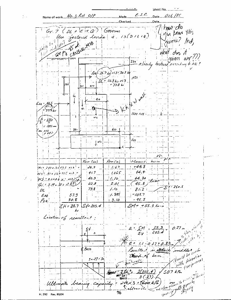
Sheet No.

Name of ^...M.±M....9lL. ..Made £ £ £ Date AtiJlL. ..Checked Date

'0

i /

\/~~ie-rn?/',f\ k/j-m ~f> J

!vii - ? ti Y.IY\•'j.r .f/• a.' r

iv?!~• ? / * AS.V .. ! „ . . : ...j : !....]

\PL \ \:\ : -

... . . J Z L / ^ . : . . . . —MJ*. - y - J ^ - i - l . . -

<->'.-"

1 £AB \ 57.3 •

\ pF<>: \ so-* 1 i ""' - 9*.S . i i i

Si/'&5.4. • " 1

-/tiurj.,<% iZu- .1 •, ill*1''/.,-... : u x . ^ : ^

----- r rr-YAL's Z/20S.4) / 5 4 7

.J «&«=}—-* 1 J^-V r-x, r . . / - r /

[...., i ! 1 i ; I d L_J L . J Sri<U/*~.- <'^-Urir^" H. 292 Rev. 80/04 ^

bheet No '.UP.

Name of work.. Made <?.:J..£:. Date <2.^C/..?.^.... Checked Date

! i v 6>O.S _ ! /.?7 >\/.ZT £C Cc->^L'7

\ ^OTKi'M '. I .[.. \yCU /fr. 43 :\wt P \ «• .1

2_ /

i

i—

! t

A-j „

- " "

•tfJtt'l /6><rAP'lUSO.\„__ 34*7 m a ) ? . . \ ' ..^1... '. :

-'One;.-,

J/>?/ri.. Starts}UsJt

• • ' ^ . ;. 'I

*• 7^.3 ._J i ' • ! . . . . . ! • . ' j

: . . . j _2S. . 0 • 0

I i : 1 «

....

H. 292 Rev. 80/04

bheet No

Name of work M?.:J.JJ...°/.£. Made D a t e . . . ^ / < ? , 5

Checked Date

2£v

6.'o

1

J

i -As - M . _

n • \ 0 C&cA

it..

._ 'II

: ._;._:__!.. 1 : : ; .„ j . „ . . '

'• ' ^M(?3<rt) ^A^rJ e{- {Ju/. ' _

Me*.*.. <.3/r£l^A(.^..$...t..J%*A <ifZU.I~|—:

H. 292 Rev. 80/04

2

. . w S h e e t N q

Name of work AiA.P..:..5.A(/...j/.€.. Made &£'A. Date C7.uk../.&.... Checked Date

l> o. &

79' ; < JL% - ?/

;_: J.U

H. 292 Rev. 80/04

Name of work ^,.AM...o/£. — •• onuut i w r..r

.Made 4?.:.^:.$:. Date.. Checked Date

5b - . • • •-] ' : :

M - ! • H-i \ : \ ; • ! ' V G" A * 0.2.x * 523

• ' I i ' 1 ! 7

(S.4o.2JM '67. 4oo & •£? 4o/>, • 3£o M/*- yuCt .

6,

'• : J\ * C/80) - i . /rfsoT • • Si69c ,,~ m

i i < i I ' 1

A : A i l «?/*?o. ; / • //(<- ...Cf

I I

JtcjJ i \ z r J t ' : Z I \ uJ L ^ , &

4Mf*_ _j, . . . . ... ' ' . . . ' . ' . . ! • •

17 K '

3/ ' df- ^

«• / . ^ ^ 2C0t)J. W / . t f / . / . 5 . . ^ 5 i ' 1 . . . ••*'/••//> • : J J : .1...: ! t _ , ' .

- ! - - ! -

H . 292 Rev. 80 /04

. 1

"Too

Sheet No. -i>/

Name of work °J£. Made D a t e . . . . ^ / ^ . . Checked Date

'j'xt?z.$fo - 2./4-ZC, ' Ms,,, Spa.

i i

///2-*fr Jj >77\Mf* jf Xo (r y 4<?i

I

"sz * /85'' A<*/4»66 6,

• 4 A i

A /8s~x/o 39o4o~

| 3 4- 74 A / A f S.!>\ ,

: 2 -

1 1

-H-_ i _ _ L _ .

_; !._]...__!

292 Rev. 80/04

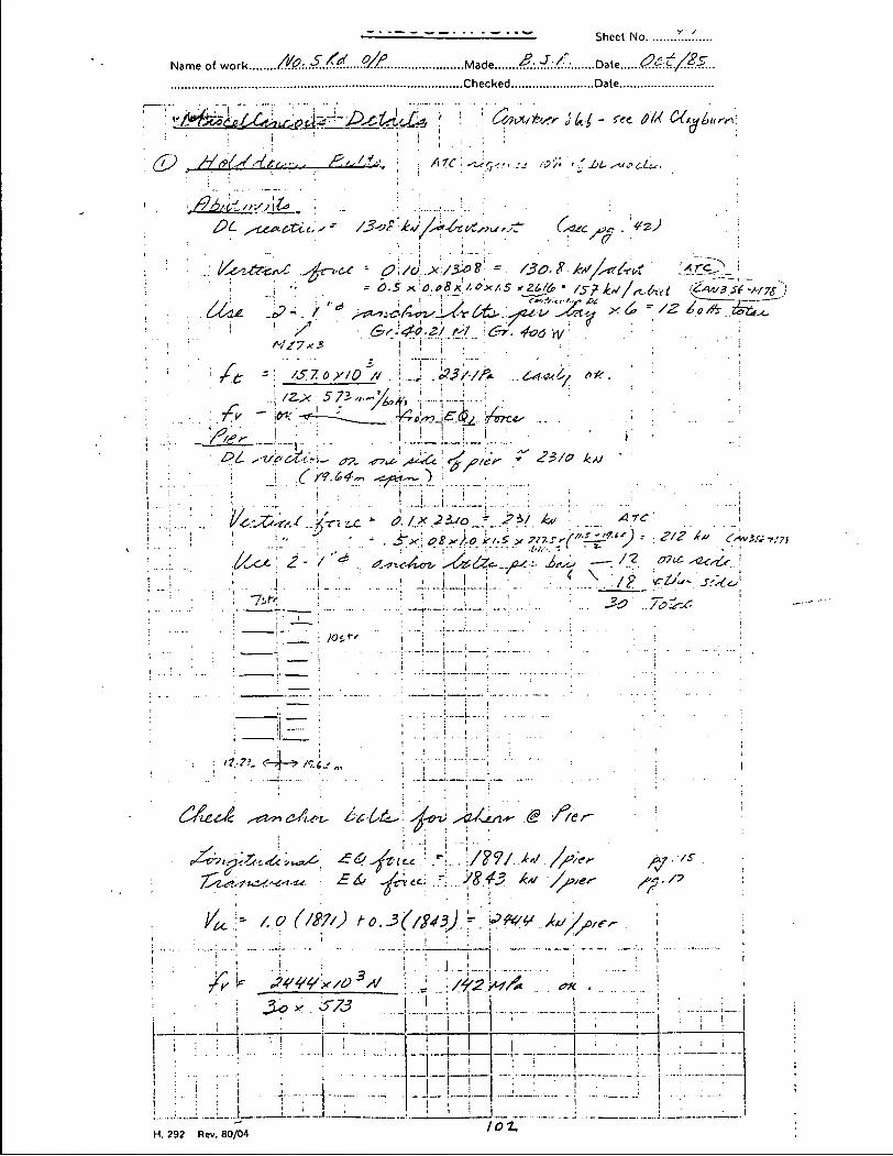
Name of work Made Z.J.A

Checked Date

Sheet No

Date

' • • ' • \ i i ! ; : i

\ \ '; = 6-S x0-*8x A**'5.*J£^ ' SS? k^/^/ml (ZAV3S( -W7SJ

'• ! " '/ &s)4-0.ZI A-V err. <k>G Yi/ ' 1

j .^3/•//'*• . ^ s f y t,*.

'V i F T ' " ' 1 A '

" 21/0 JcAJ

A-rc '

. . . . . . . . . . .... . . .. ...... I - X-

i . ; . . ' i .l_j._L_j_. •.. : . /? '\et/~ sUJ

it.-?'-. c-A-y

p^>g<Zc<6'>ux^, £ 6 . sftit-c ' r\ \/?7/ A*/ Tsi^tst-uzf.^c*-**-- ~^cxta,"\..s.B.4-3. .6*t /y?/es-

ft •<;./7

7^ I6" fVW'*/03*/

! I

I

H. 292 Rev. 80/04 /Ol,

PROBLEMS

CLASS

NAME DATE

l/MlT 5r/f7€S tefeA/

A/0. & £oAO B&*6£ /)&>TMBMT

LSD faktAcfterz \

P R O B L E M S

N A M E tyjjyyec/ 1

61

I

if-

i

±

6 ^

4 / o

5>

o

D A T E / W / ?

/of

P R O B L E M S fa C L A S S

N A M E DATE ^Jcft+e. 9./T9/

L A

S" »*f> + A ^ f fefainrr- fj? fare*.

- 0.2. 22V«r * 12.. o

^pr /oo/L a/So ^ ^ c M tTXefafO

P R O B L E M S ¥4 / ^ . T / ^ /^/m/- C L A S S

NAME

St'fe, Ccetfftfrv??'—> 6~x>#'cn^ So,Y fart/-*- J?/3* ST - 32

#Y. f SUsi^fo ft rears /tSotfwrtfe f £e6*tf*p Us#/&.

So/7 fHSSt/ftS ont 4* LXKJ~ °£ aJx//ryT'«rL- (*ar//S.

/ . /ty*mrr ? </18 ~ ?8 I

Al-O .' -*/*./>L 4*\*£jSlS.

PAe-r°AfAPAe — * A-P*Pk) + t h e LQ4H) PAL

fa - v*-V as.

I r " rs ~f .

0 0 ^ CA>t£g$tyt)a*(g£-) J

P R O B L E M S

AS/)' *J0.S£cL Abufv*+*t C L A S S

D A T E 3ty/ie. 7. AJ^I

<?/&<!>{ /e&it' 7^oA>yS : /• 2.S" C**l Cc*n/>o u>f/4 'J-****) . 0&

e/tad /*W-' c*s A/>/*<*• "he**** A 2 a e«r*h 6'/1 A*-!?

£«<rtk fissure t

/k> cA 4// JTSJ*/ rc

6-Jo

A 2 S

A/O

OS 6-8

z=- oc.

<*rP + A ° ' BQ

5 ( _ £ 2 . 0.90 • i—

FLS I - AO - L

U(S —/fic/brrd res/sAtM* */t*>«yS cxc^st/sr ti/b/ A*c/i>v*o/ /oatef.

SLS

£ *"*y/to«*n or *»/«*"">« Ao*c/. fab** A< «s<* A>

a. t/*/u? oA /.OO &AtuM Ac upta? fi<&

- M C»/e> i A DctclA?/ frrseut! «/^»« "*/«C< Ao**A -eAKrcfr

> I t i l . . yj^^j,*/

P R O B L E M S

LSD- /VO* C L A S S

D A T E Tune. /<?./?,??

Jit V-C t-oacf: fat*. /octet fn*rx WSJ fa/cUs/fr/fonT.

£LL - 3</t AAJ j?,,- fa fife

/hr\ t>f- <»A{/>y\rtiT

Ca/c#/*fe //is*" /octal

/}/>s/jr\ Lows: tJt* •> Z%tLj ^ ' ^ ^ '

-^vouXoL c/uo/c jXJc

t H

.90 ' f ty t* p H \

1*

{ft

0 /oo loo HO \u <,M,/W

i l l \ \ I***

PROBLEMS

LSQ - AJo.G-fo/ A&jAriMt CLASS

Truck. U>CiA\n^.\ \-\(

t 1 I?

£ rA ? o

/ I

£A ( ( 2 - ; = . £ V > 0 2 ) • * ll!s(5H) + I ^ U Z ) Co-fe)

6.G L 4s I

t

^ ( / i ) ( j f iD" )^ ) *- fall.-?)

H i

/ s s - . t

PA

^•(1^75 + Mir* V^o

P R O B L E M S

C L A S S

N A M E

£ / W 5 0 ^ (drttejn /afVs)

2 5

/ /0

PROBLEMS AS/).

L I 0 0 0

<• >f

j ,V3>

_3f i 50«

Mo.

- cA<ck j»f-h 4*fremei *ac/i Case.

W

fcj^f" of* S»jf (fvitn pay m.) fnc/ sutrcfi*rf>

CcH-BJX,

150 -/2SO

U<*nnj Ce*f»C4'7y : b- 3^20 tnrv, *• &O0 sunAmty. cast, J.

= &08t:

P R O B L E M S LSD ftps./Coetd 0tfrp&- /9£//hlfnf' C L A S S

DATE JT/m,

4 - n / V -

4&- 5 / 7

22. v 37. V

.0

Lfarl/tj C<xf*toAy : D - foZo + &OOtr\m scrrtturret- &~ I

fry—

hu* 52<b )°J^

Lid

PA**

— Tun-

$.6 k,uh

III-

P R O B L E M S LSD Pant. IQ CLASS

Bad to

We*,,* = 76-6 /Af,

4m,4 * 3*4/*/, '7.1

6> 'AM,

/ W * /.z(io-fi)*/i*+ /.its6-6)+

MM}***, *0,Z L**cf r i .1\ | M . . . . . . . | [A ) i. i I

Ito

1 D*1

22. (, #

27. oH 37. /. ohS

S-7,/3' -z., 0 1

/ .D)

A 2.

* ~ / . 2-/

1,1-''2(- -0,11

3

ttiu//twf ll I in

113

PROBLEMS

/Vo ST 4na*f /fa* P> CLASS

NAME

Al/AJ/pC/M SOIL; fSOBL-

O A T E .Ten, ff /Iff.

Ph«,~=. -$6>2. LP*

£ It kI±lDj

14*1 k m effsfr ^ 2 ~" 'P> -2.2 L/o)

£—^ yr// / / ////

w , \A/i,

l.il <•/7.80

AolS

Z.o 1 0-ZoS

/S/.o&> J.

KJH - /> 2" 0

•'f HJu/L*\ A >r\ i i / X < ^ ^ • /S >

•2-2-

/W* I7S.S' /LP*s

P»>,* - <-1%l I P^

fL""ilr"y—ff

Iff. / M

P R O B L E M S fa Ah £- fio*d 4rtdy- AA//Ue*f C L A S S

D A T E .Tuny 91

but

tffhjfyu/fn So// Levsi/

f ^F v=: 28Z-.7 is-iV/,.

282 °>

\ S-^W. ,1.0

4

iq* (/-£.}*• * (1-1* )*= e-tel 10

3? o..607

/26Z>7 + 279,/

/S6Z.0 IP* r 4 2-7<5._/

» jieojij.fi*

t

us-

V

P R O B L E M S LSD 1 / S y - / 3

Ah S /fogcC Ariofy- rfAsfa** ? CLASS

NAME

Maxfnlttfn ^o'lf i-ft/t(

a 7&- 20

r

i

D- f.6Z ryy t*i'/t St/rtfirry. £ ' = $770 APx*

\ fa2 lS.J

'f~ ft - II.-"'. ^ - s.zi3 33

rir-f.n + -25 8,/$

f

faojvrtd. fastefaws: (^acfrn^ o-sl

/Y>/w#)ttm hoi/ /mi 7B/ / / V -

T

12>Z IP*.

f\<S/S-hr?0€.

M/htwum so/'f /tut,/ id \ > >

ok.

PROBLEMS ZSZ) 1 / W / V

CtfBPC

• fft+tar cA/sfr/JhAhi of £0nfac/^/rsstrra sfo// As arsswtf

^ - se*ufice of CtmsAvcficrn rcftcr**** /1 ^arram* fit's a cvnst^H&Ce of ctmfacAovi

— oismfafions » f */*6r»THf}'ar> of sct/eAvcSum $jr*,t'/o*~

Sc4b$UrfcrC< COnp///>er>% - M{fut*C€ of so)/ i/an'a&i'/ffy /^/uc/f'^a /cy+ri' - i'nc/tic*cJ s^rfss tsfintM /tw/s /» re&fi'on fo /fre u//fn*fe.

t^s/ifcrrtce. t ^artctnso/tt/aAtfn p assure. — permfa/Sr'/ij^, c/m/n*2< ooyv/tnfn , uafrr con/m? r pone, /xssvne - me>u»n,'fa/c. of the sPhr/ins f* /A* so'& assoc/ci/bef c*/M /A*

— censo/'efarien, ere*/*, jote/Aty, or c*t/*fS<. cjtcr*c/rr-/sf>'cs.

-^&/}'vrvtfrs of ^fos/>C $etffr#H'*t/s of s£vi//o«v fcunt/o-flWS

' /2-- 2- 2. ' ' 3 J = O.-S-

g r o-53

Tabic

I0-2S fifalL $0-0

111

- SI3&4 ^

- \2-o ooo •<

LSD /Lb S-&C My AJ-

Pay*. /£T.

C L A S S

tc' 10

E ,

^7

f ^ S~ w\

fO /v ) •>->

/ S " t*tvn

25" « n n

'SO i t w

7©

I (&>'

2 2 6

3fc |. S 7 V/ 3 ^

6Zo 7 2 3 $2t

/o33

0 6.1 ~ (7..Z)l+&>)

^ 1^ £nr\m pf StfYfrms/rf &

fa SL<> C U i/'oMst) j / A e .

£J< / ' / ' ' ' jy 'Ae

Ves^rr*/^ {fa

1 //fi U /, NOT oj-

PROBLEMS

A/o.S fact/ AfuAv*/ /6.

CLASS

727 (U$t rr\/mrwu*yJ fo fas

6^

)/trb'Cct / /orz/s .

* ( 2 7 . 7 + 0 w + r3f,°) Ufi-b. 10-9 r 76.6 /»>6/-» •

/) A -(tj)(/*)(f*n 33 j

fa - S7.7S /LM/n

/rfy« 3-7.1

stxtuefp ^ t * ^ / K W ^ I , ~~~

P. II?

PROBLEMS LSD AL /[/{>. S AtaeC Sriet^ A&mf. CLASS

*MonA*'ou I DATE ^SsnS //, / f f f

Load ^ A2S-(£) =r /.£3-(/>A)

/ /?0 £CMchainy<. J

2 #2

2 0 A * / >

5 ^ i i/wyU

i'i b i / i / f

~/6/UM Snt6( <c£ vac*? 0tf b/c. *r<*? *^{**ytMr>asy. st/ifaZeov^

^ t * * ^ sctcAc-ijc i+ ytOUj ojj %et*n.fi> fit. <3A .

— ^ cf/So/ fact, siof- /nctiayfayt' eCtecffC/o**f^ Au/~ /6ti sarSfj }f cvobt/eC A C / as f*r/ 0 ^ /A*.

\jj , x ^ f a m xuF w

P R O B L E M S LSD ML C L A S S

- /.As- E + /'O f=q>.

if «ll % ~

0 ^ uetf+•* soil + »fat"** / / K - * 3 7 . X

3) /icAtcfc fass/'u-c puss**--

C^*e>fa&/)

fOcss/^ p*5svre. 'cfs /n opposite S''*cA* t^** tfa

-aSossWs rr^ayr}/ stout M am^nt**- r? /o*cfir>j ? £ ^ .off) rf^*'/ PUlL+Umt«/»*+«f ~/+jtssf

,W lO, Sviiijt pw«**

/2s (&/) + />°ll>6)

12-1

)

P R O B L E M S /~sj> AM. ^ MbocAryi^tS C L A S S

NAME DATE

\/trb'c«( -fires - / ^ - ^ of *r

I Z 2 .

Yl-hrcimfa/ EgsisM^c^ Mcke//'\A P R O B L E M S /2><v 2£

Yl-hrcimfa/ EgsisM^c^ Mcke//'\A lbQ/-2,- Q?S>Hf\WL£ • C L A S S Yl-hrcimfa/ EgsisM^c^ Mcke//'\A NAME S^U^t^/Os DATE. 7 ^

I B J I M I J I H , | l i r i . i i a . . . » , - l . , . « i U i M , . l , - m . ^ ^ ^ /

l>

fie* 33-71")*"

y /

Ifr31.2. W'

P , 17-7.-?-W*-

~- /of, os A*/^

IZS

P R O B L E M S .

J 7 T

O L S. J L — = 5 > err? 6<*yj wsr r M

Z1

A Octet - OO/f-h i- uoffAoUtf fes/hz/r>s^ f&<rC-£. .

(JL S j2- Stfafo —> / far/etc? /roc /Y<* £S<?(

' Su&sMjoff-p^SS/u^

Sub r 3 s / ^ V

PROBLEMS /a W 2 2 -/foe/ivOTAC- fcvsr/lAJCe. CLASS

/- Qa t>f

/( 12') . 5 5 , £ - w . ......

M-t' --(6 ) / 2 2 j - 3?. z A AI/,*

F £~o«at

> Tr'- /0-2.2.

# not: Ete'w di'd Atk v* k> 1*A of p«t/V-t A ^ M I * . ^ /j ^ ^ M ^ ^

*6> fan c/vdt

&%>j- 3$b t os(/^.o) ' 108,IsO kHJfo

56.1 k^/l*-

tzar

P R O B L E M S 2z 2 C L A S S

7*$<L S3'S - ULSS

/' . Jhssite - 121.1 hI*/^ <#>^L fvy 7?r-2,OQhi I'

f Mif'- SS-S- / 6-S {/27. 7) Hr / fJjjfr ^ 1 ^ 0 ^

/o/,o A/j/m h'

» 5^^> / +- pars*'**-'

>

life

PROBLEMS

fbflfiOUTAL _ tevSTAMtE. CLASS

f

?fe* 7o, 1

Ass*** 76.6 f- 0>-%-&) ~- 61.1 kNJ^

UL^> sr

<0 Z. t i*>l„ > FL M «" Si- 3

i n

P R O B L E M S Da*,*. 26

LOL^E—^ Sc/Sno/h C L A S S

N A M E 6y0/t7)**SsX s D A T E ^7Z^?n/, Z>9 —- • / 1/

Sect'**,

i>*t.S'\l Wn/nutm Ala/ys/s fo^'/rwesih & Mu/f?-Spq» Pntips.

ft C/kSS/'&'f cmty c& "'oirh-er bridp/5" , n

¥

(I

i. Y.l.(

11 ff t l

S,'tc Coefficient So*// /Vcf t /s 7y[U. UH

M M

fzfasfi^ £z./s**i/c Respw'ye. Coefficient

e-fasflc s&sm/c fact = Cz^W

T a / 3

^ 2-s Al

YY./O-f

=. lot/Wot/ p/^tzA .

— s/njle. -^poi^i kricdjes • wi'^/mum dss/jn ct>^^ct>'i^\ •forte.

foo /so

fyp^t /f^h, AJ. fas. o/cu/ttlcjL <?/WJ,

128

//C>£/2£V\JTAL-

PROBLEMS

S~e>S>pic CLASS

NAME DATE C7Z//K. -Z9. JW

-r-asf^ik^rs s(\a/( oAssAftifoA /> -insure in-fejri'L t / / * * ^

— 3* A (fond- k>*d- c£ th*- /'jbkis- 'Ai-tu. £ 0<S/'om/s^ )

fcoT 3 h > O. 2. * A)WfD r

fcoT 3 ft > O. 2.

¥ /\n fvus a A< Ar,/>n1

-

" B/w 1—1 L

•/fa. rftfr*'***- face" - 2*A*vLY £ L •»- o Aspen -

by - 2 - 7 3 0 - //^^

Af <S4- P^- o.zAy /? = 0 . 2. 5 ^

w^/^-V #/" +A»Ac*>*A . •= j0r& /cAj/„v <=-r- A An ,\ Ate AAjhA"Y~ tA Ahe 2- '0<rj'ow'>y sfacA'tz . .

ce

UtA ,A n fat*' 1

aAA-ot/ Auf9 Jos/ *A

* £ A*/A Ar> s//<//fy ,

P R O B L E M S

CyQhB -» St/Sty /£• C L A S S

ISO

J <Jtoi&vmt not

/ coug • I***- fate* ~> onu., Just EG fi^^.

WLSS

0 A?a^c>L 6u<mao'.

I /2s C/%) V /' t>LW bsi)

- 2/,/) J/>0(£9-s-)

L{ A?$(3/J) + /o ( ,sy-S~+7>6)

~ /OO, A^j/r^ <

C a r t ' / h/sis,"/ SA's f

„ '/ wi/ /A* tJ&rf/!

-# tVlUsf /M */>k f° ildv^ f&Ss/lrt, frfSJul-LS fat* S-aryj* 6ooo .

tyoohi'st /}**-&•

/6<S/s/a'?C£. mUS./ wcJufi/e. pc?££'\/£- flYJJUtfS.'

^i^iditf/ *&ou/ //)€ rlfy+ri** t/ynimtc w»yxnn*+7 ? f

130

PROBLEMS

LODE—5> SfSm/k CLASS

NAME ^OOO^/n, DATE ^/t/ne 2°) 9 •• j /

PaSS/'ve. Pnssofh/S:

H=/3s

tos /foe> cos fs3>) * D. 0 236 7*

4-- 33

/£ Hi

60S — — --^-^—> f -

(33-S/7) * ^ /h ( i7 .3J

^(Wft • — r - v

131

P A E = 0 . 5 * K A E Y H 2 ( 1 - k v )

H

k*

3.52 m 19 kN/m 3

0.000 0.100

^ r 8 P

e <p

0.329

deg rad 33 0.57596 22 0.38397

0 0.00000 0 0.00000

5.7| 0.09967]

1 ^1 31.1 kN/m P A = 0.5*K A *y*H 2

| K A | Q264 |

| A P A E j 7.6 kN/m A P A E - P A E - P A

Pc*cf 21

E | 1.36|m point of total thrust (above base of abutment)

I32,

Pay; &

PE

H

Y

k v

K

PE

E

8 P e

F — r

i

127.7 kN/m P P E = 0 . 5 * K p E Y H (1-kv)

1.35 m 19 kN/m3

0.000 0.100

7.375

deg rad 33 0.57596 22 0.38397

0 0.00000 0 0.00000

5.7 0.09967

0.888702

| 140.0|kN/m P P = 0 . 5 * K p Y H

8.084

-12.3 kN/m

0.42 m

APpE - PpE " Pp

point of total thrust (above base of abutment)

check these results - max passive resistance should be decreased when the dynamic component is added in.

)

| 33

Appendix C

134

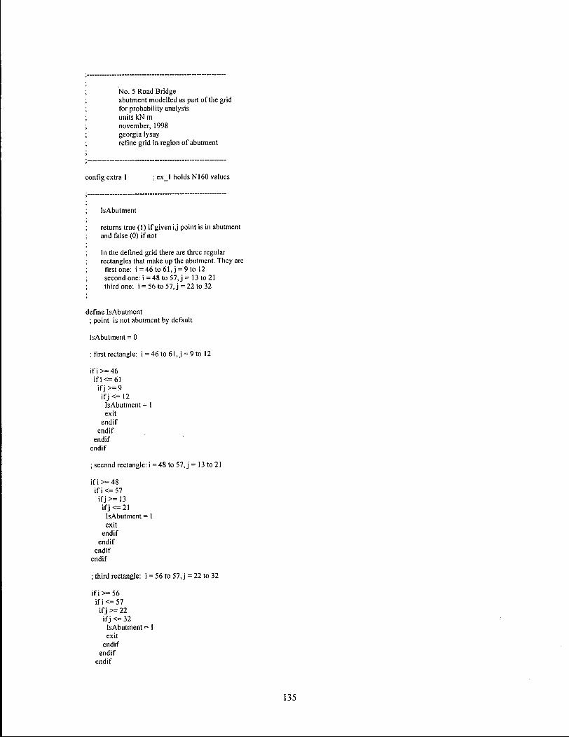
No. 5 Road Bridge abutment modelled as part of the grid for probability analysis units kN m november, 1998 georgia lysay refine grid in region of abutment

config extra 1 ; ex_l holds N160 values

IsAbutment

returns true (1) if given i j point is in abutment and false (0) if not

In the defined grid there are three regular rectangles that make up the abutment. They are

first one: i = 46 to 61, j = 9 to 12 second one:i = 48 to 57, j = 13 to 21 third one: i = 56 to 57, j = 22 to 32

define IsAbutment ; point is not abutment by default

IsAbutment = 0

; first rectangle: i = 46 to 61, j = 9 to 12

i f i >=46 i f i<=61

if j >= 9 if j <= 12

IsAbutment = 1 exit

endif endif

endif endif

; second rectangle: i =48 to 57, j = 13 to 21

i f i>=48 i f i<=57 if j >= 13 i f j<=21 IsAbutment = 1 exit

endif endif

endif endif

; third rectangle: i = 56 to 57, j = 22 to 32

i f i>=56 i f i <=57 if j >= 22 i f j <= 32 IsAbutment = 1 exit

endif endif

endif

endif end

SetAbutmentProps

define SetAbutmentProps shear_mod(i j ) = 1E6 bu lkmod( i j ) = 1E6 density(ij) = 2.5 friction(ij) =45 cohesion(ij) = 1000

end

SetSoilProps

define SetSoilProps mean = 12 ; N160 is defined as a normal random stddev = 3 ; variable with the given mean and nl_60 = stddev * grand + mean ; standard deviation i f n l_60<0 .0

command print nl_60

endcommand n 1 _60=mean

endif atm = 100.0 ; atmospheric pressure (kPa)

mean_stress = abs(((syy(i j ) + sxx(i j ) + szz(i j))/3)) mean_stress = max(tnean_stress, 0.02 * atm)

gmax = 440.0 * (nl_60A0.333333) * atm * sqrt(mean_stress/atm)

sfactor = 0.09 bfactor = 0.27

shear_mod(i j ) = sfactor * gmax bulk_mod(i j ) = bfactor * gmax ;density(ij) = 1.8 ;friction(i j ) = 36 cohesion(i j ) = 0

end

SetlnitialProps

set the initial properties for all i j points

define SetlnitialProps loop i (l,izones)

loopj (1 jzones) if IsAbutment = 0

SetSoilProps else

SetAbutmentProps endif

endloop endloop

end

Flac commands

136

; grid generation grid 73,32 model mohr

initial x = 0.00 i = 1 initial x = 0.15 i = 2 initial x = 0.30 i = 3 initial x = 0.45 i = 4 initial x = 0.60 i = 5 initial x = 0.75 i = 6 initial x = 0.90 i = 7 initial X = 1.05 i = 8 initial X = 1.20 i = 9 initial X = 1.35 i = 10 initial X = 1.50 i = 11 initial X = 1.65 i = 12 initial X = 1.80 i = 13 initial X = 1.95 i = 14 initial X = 2.10 i = 15 initial X = 2.25 i = 16 initial X = 2.40 i = 17 initial X = 2.55 i = 18 initial X = 2.70 i = 19 initial X = 2.85 i = 20 initial x - 3.00 i = 21 initial X = 3.15 i = 22 initial X = 3.30 i = 23 initial X = 3.45 i = 24 initial X = 3.60 i = 25 initial X = 3.75 i = 26 initial X = 3.90 i = 27 initial X = 4.05 i = 28 initial X = 4.20 i = 29 initial X = 4.35 i = 30 initial X = 4.50 i = 31 initial X = 4.65 i = 32 initial X = 4.80 i = 33 initial X = 4.95 i = 34 initial X = 5.10 i = 35 initial X = 5.25 i = 36 initial X = 5.40 i = 37 initial X = 5.55 i = 38 initial X = 5.70 i = 39 initial X = 5.85 i = 40 initial x 6.00 i = 41 initial X = 6.15 i = 42 initial X = 6.30 i = 43 initial X = 6.45 i = 44 initial X = 6.60 i = 45 initial X = 6.75 i = 46 initial X = 6.90 i = 47 initial X = 7.05 i = 48 initial X = 7.20 i = 49 initial X = 7.35 i = 50 initial X = 7.50 i = 51 initial X = 7.65 i = 52 initial X = 7.80 i = 53 initial X = 7.95 i = 54 initial X = 8.10 i = 55 initial X = 8.25 i = 56 initial X = 8.40 i = 57 initial X = 8.55 i = 58 initial X = 8.70 i = 59 initial X = 8.85 i = 60 initial X = 9.00 i = 61 initial X = 9.15 i = 62 initial X = 9.30 i = 63 initial X = 9.47 i = 64 initial X = 9.67 i = 65

137

initial x = 9.90 i = 66 initial x = 10.16 i = 67 initial x = 10.46 i = 68 initial x = 10.81 i = 69 initial x = 11.21 i = 70 initial x = 11.67 i = 71 initial X = 12.20 i = 72 initial X = 12.80 i = 73 initial X = 13.50 i = 74

initial y = 0.000 j = 1 initial y = 0.491 j = 2 initial y = 0.890 j = 3 initial y = 1.237 j = 4 initial y = 1.539 j = 5 initial y = 1.801 j = 6 initial y = 2.029 j = 7 initial y = 2.228 j = 8 initial y = 2.400 j = 9 initial y = 2.550 j = 10 initial y = 2.700 j = 11 initial y = 2.850 j = 12 initial y = 3.000 j = 13 initial y = 3.150 j = 14 initial y = 3.300 j = 15 initial y = 3.450 j = 16 initial y = 3.600 j = 17 initial y = 3.750 j = 18 initial y = 3.900 j = 19 initial y = 4.050 j = 20 initial y = 4.200 j = 21 initial y = 4.350 j = 22 initial y = 4.500 j = 23 initial y = 4.650 j = 24 initial y = 4.800 j = 25 initial y = 4.950 j = 26 initial y = 5.100 j = 27 initial y = 5.250 j = 28 initial y = 5.400 j = 29 initial y = 5.550 j = 30 initial y = 5.700 j = 31 initial y = 5.850 j = 32 initial y = 6.000 j = 33

gen line 0.0,0.0 5.7,3.75 ;line 1 gen line 5.7,3.75 7.05,3.75 ;line 2 gen line 7.05,3.75 7.05,4.35 ;line 3 gen line 7.05,4.35 8.25,4.35 ;line 4 gen line 8.25,4.35 8.25,6.0 ;line 5

model null region 1,30

fix x i=74 fix x,y j=l ;fix x i=56 j=33 ;might have to fix top of abutment check this ; set properties prop fric 36 rdev 2 density 1.8 rdev 0.1

SetlnitialProps ; turn on gravity set gravity=9.81 ; histories hist ydis i=52 j=22 ; top of abutment hist ydis i=54 j=8 ; bottom of abutment hist syy i=54 j=8 hist unbal hist shear_mod ; load abutment incrementally step 2500 ;solve force=5e-2

138

ini xdisp=0.0 ydisp=0.0 ;set large ; try this file also with small geometry apply yforce—50 i=52 j=22 step 5000 ;solve force=5e-2 save l_50.sav

apply yforce=-75 i=52j=22 step 5000 ;solve force=5e-2 save 6_75.sav

apply yforce—100 i=52j=22 step 5000 ;solve force=5e-2 save 6_!00.sav

apply yforce=-l 10 i=52j=22 step 5000 ;solve force=5e-2 save 6_1 lO.sav

apply yforce=-120 i=52j=22 step 5000 ;solve force=5e-2 save 6_120.sav

apply yforce=-130 i=52j=22 step 5000 ;solve force=5e-2 save 6_130.sav

apply yforce—140 i=52j=22 step 5000 ;solve force=5e-2 save 6_140.sav

apply yforce=-150 i=52 j=22 step 5000 ;solve force=5e-2 save 6_150.sav

apply yforce—160 i=52 j=22 step 5000 ;solve force=5e-2 save 6_160.sav

apply yforce—170 i=52j=22 step 5000 ;solve force=5e-2 save 6_170.sav

apply yforce=-180 i=52 j=22 step 5000 ;solve force=5e-2 save 6_180.sav

apply yforce—190 i=52j=22 step 5000 ;solve force=5e-2 save 6_190.sav

139

USER.FOR for RELAN Analysis

C *** USER SUBROUTINE FOR ABUTMENT PROBLEM C C

SUBROUTINE DETERM (IMODE) C

IMPLICIT REAL*8 (A - H, O - Z) COMMON /CL/ GAMMA, MEANL WRITE(*,100)

100 FORMAT(/' ENTER GAMMA V) READ(V) GAMMA WRITE(*,200)

200 FORMAT(/' ENTER MEAN LIVE LOAD 7) READ(*,*) MEANL RETURN END

C SUBROUTINE GFUN (X, N, IMODE, GXP)

C IMPLICIT REAL*8 (A - H, O - Z) DIMENSION X(N) COMMON /CL/ GAMMA, MEANL GXP = X(l) - ( MEANL * ((X(2)*GAMMA) + X(3))) RETURN END

C SUBROUTINE DFUN (X, N, IMODE, DELTA)

C IMPLICIT REAL*8 (A - H, O - Z) DIMENSION X(N), DELTAfN) RETURN END

C SUBROUTINE D2FUN (X, N, IMODE, D2, N2)

C IMPLICIT REAL*8 (A - H, O - Z) DIMENSION X(N), D2(N2,N2) RETURN END

C

140

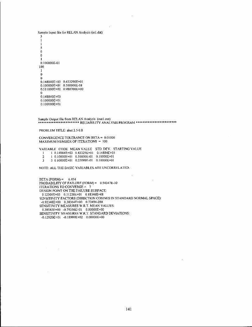
Sample Input file for R E L A N Analysis (inl 3 1 1 5 0 0 1 0.100000E-01

100

dat)

0 0 0.148840E+03 0.100000E+01 0.511000E+02 0 0.148840E+03 0.100000E+01 0.100000E+01

0.433290E+01 0.500000E-01 0.988700E+00

Sample Output file from R E L A N Analysis (outl .out) * * * * * * * * * * * * * * * * * * * * * * * * REL IAB IL ITY A N A L Y S I S P R O G R A M * * * * * * * * * * * * * * * *

P R O B L E M TITLE: abut 2.5 0.8

C O N V E R G E N C E T O L E R A N C E ON B E T A = 0.01000 M A X I M U M N U M B E R OF ITERATIONS = 100

V A R I A B L E C O D E M E A N V A L U E STD. DEV . STARTING V A L U E 1 1 0.14884E+03 0.43329E+01 0.14884E+03 2 1 0.10000E+01 0.50000E-01 0.10000E+01 3 5 0.I000OE+OI 0.25099E-01 0.10000E+01

N O T E : A L L T H E BASIC V A R I A B L E S A R E U N C O R R E L A T E D .

B E T A (FORM) = 6.454 P R O B A B I L I T Y OF F A I L U R E (FORM) = 0.54347E-10 ITERATIONS TO C O N V E R G E = 7 DESIGN POINT O N T H E F A I L U R E S U R F A C E :

0.12301E+03 0.11238E+01 0.18346E+01 SENSITIVITY F A C T O R S (DIRECTION COSINES IN S T A N D A R D N O R M A L SPACE) :

-0.92348E+00 0.38364E+00 0.73494-288 SENSITIVITY M E A S U R E S W.R.T. M E A N V A L U E S :

0.38585E+00 -0.79356E+01 O.O0000E+00 SENSITIVITY M E A S U R E S W.R.T. S T A N D A R D DEVIATIONS:

-0.12920E+01 -0.18999E+02 0.00000E+00

141

1

o o o o o o o o o o o mmuiioininmiflinmu)

o o o o o o o o o o o oocqcocqcqcqcooooooooo CN C\i CN CN CN CN CN CN CN CN CN

m o m o i n o i f i o i n o c M M n N O M n t M O S i n d j O i M n n o c o o T T - c j ) c ocNr ^ ' c N r^c \ i c o T- :(C ) T - ' i r i

^ • r - ' - O U D C M C M ' - N f f l T -( D O W i - s n M O c o c o i r j o i n c o n r o s c o i - o o r M c M c o i n c o i - o i c o N f o i o u C O C N C N C N C N i - T - T - T - T - T -

lO O O O O O O O O O O It > o (->

o o o o o o o o o o o o i q o i o o i o o i o o i o o

^ ^ ' l o ' t r i c b c b r ^ r ^ c o c d a i

l o i n m i o m i A i a i n i n i o i n t— r-~ t~~ r—

N S S S S S S S S N N o)0)0)a>a>o>cncncncna) o o o o o o o o o o o i ^ S : r « . i > « . h « . r « . r « . | v . h . f s . ^ w i A v i i A i n u j i o i f l i n i r i u ) C N C N C N C N C N C N C N C N C N C N C N

M n N O S l f l t N O M O T - c o r - ~ c o m r o c N T - o o o r - ~ Q j O J c o N i D i n T r n c M O O ) c o c o c d c o c a c r > < x > c o c o c o r - ~

f T U ) l O ( D ( O N S C O C O

\u> j II > o u

r-~ CN CN CO CNI CO T J -

CN O O CO LO CD ^J* T - o n (D s \r t o T r-~ •<- co CN a> CD cq i n t o ^ - co co o o o ci o o o

T - co T -O (D N O CN O T - t o rr CN O CO CO CO CO CN o o d d

O UO o i o o t o o O CN t o [— O CN LO CN CN CN CN CO CO CO

O LO O O CN LO ^

C O N S S C O S N S C O N S oocooooooooocooooooooo cocooocococooooocooooo cncncncncncncncncncno) O O O O O O O O O O O

r O T - f O i - f O r - f O C N C O C M f O

mmmuiinifl ininininin ^ a i c o r ^ c N C D ^ t o o ' k r b o

^t- ^t- m r o r \ i r v i — /—\ /-t>

i - N O l i n i O C M T f O T - S

• r CO CO CN CN aii o i o i

^ to to ID CD

T — O CT)

CT) 0 0 r-~ r - co co

I IO I CN I li > o

o

O O O C O t f f l i - S T f M O O ^ T O C O C O C N C M T - O I O C D O ) I O C D C N C N T - C N O

- . r O N r g t o c o c o c o ^ O N i . r - q O l C O S S C D t D l D l O

o c O L o c o o c o t n c o o c o t o O T - C N C O t O C D r - ~ C O O T - C N

CN CN CN

O L o o i o o i o o i o o i o o ^ " " T i n i f i C O l O S S C O C O O )

142

Append ix D

143

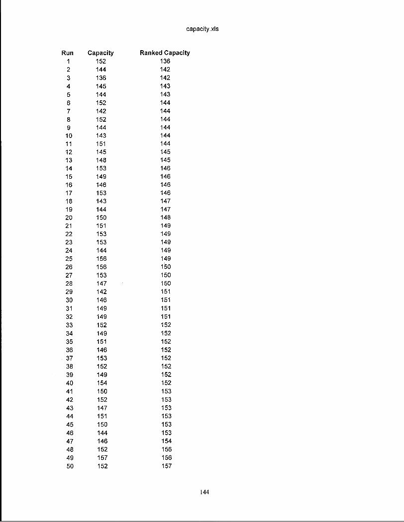
capacity.xls

Run Capacity Ranked Capacity 1 152 136 2 144 142 3 136 142 4 145 143 5 144 143 6 152 144 7 142 144 8 152 144 9 144 144 10 143 144 11 151 144 12 145 145 13 148 145 14 153 146 15 149 146 16 146 146 17 153 146 18 143 147 19 144 147 20 150 148 21 151 149 22 153 149 23 153 149 24 144 149 25 156 149 26 156 150 27 153 150 28 147 150 29 142 151 30 146 151 31 149 151 32 149 151 33 152 152 34 149 152 35 151 152 36 146 152 37 153 152 38 152 152 39 149 152 40 154 152 41 150 153 42 152 153 43 147 153 44 151 153 45 150 153 46 144 153 47 146 154 48 152 156 49 157 156 50 152 157

144

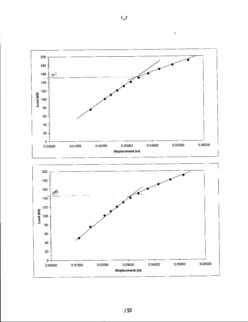
3 4

40 -f

20 o I 1 1 1 1 1 1

0.00000 0.01000 0.02000 0.03000 0.04000 0.05000 0.06000

displacement (m)

200 -r ^ •

180 -

160 -

140 -

_ 120 -z

^ 100 -0 '.

80 -'•

60 -

40 -

20

0 '. 1 1 1 1 1

0.00000 0.01000 0.02000 0.03000 0.04000 0.05000 0.06000

displacement (m)

5 6

0.00000 0.01000 0.02000 0.03000 0.04000 0.05000 0.06000 displacement (m)

20 -:

0 + 1 1 1 -t 1

0.00000 0.01000 0.02000 0.03000 0.04000 0.05000 0.06000 displacement (m)

1

0 _£ 1 1 1 1 1 1

0.00000 0.01000 0.02000 0.03000 0.04000 0.05000 0.06000 displacement (m)

40 -f

20 -f

0.00000 0.01000 0.02000 0.03000 0.04000 0.05000 0.06000 displacement (m)

9 10

1 2

20 f

0.00000 0.01000 0.02000 0.03000 0.04000 0.05000 0.06000 displacement (m)

ISO

\

1

0.00000 0.01000 0.02000 0.03000 0.04000 0.05000 0.06000 displacement (m)

0.00000 0.01000 0.02000 0.03000 0.04000 0.05000 0.06000 displacement (m)

7 8

0 -F 1 1 1 < • ' 1

0.00000 0.01000 0.02000 0.03000 0.04000 0.05000 0.06000 displacement (m)

20 +

0.00000 0.00500 0.01000 0.01500 0.02000 0.02500 0.03000 0.03500 0.04000 0.04500 0.05000 displacement (m)

I S3

9 10

20 +

o x 1 1 1 1 1 1

0.00000 0.01000 0.02000 0.03000 0.04000 0.05000 0.06000

displacement (m)

20 +

0.00000 0.01000 0.02000 0.03000 0.04000 0.05000 0.06000

displacement (m)

11_12

0.00000 0.01000 0.02000 0.03000 0.04000 0.05000 0.06000

displacement (m)

200

0.00000 0.01000 0.02000 0.03000 0.04000 0.05000 0.06000

displacement (m)

issr

13 14

0.00000 0.01000 0.02000 0.03000 0.04000 0.05000 0.06000

displacement (m)

0.00000 0.01000 0.02000 0.03000 0.04000 0.05000 0.06000

displacement (m)

15 16

20

o I 1 1 1 1 1

0.00000 0.01000 0.02000 0.03000 0.04000 0.05000 0.06000

displacement (m)

151

17 18

158

19 20

0.00000 0.01000 0.02000 0.03000 0.04000 0.05000 0.06000 displacement (m)

0.00000 0.01000 0.02000 0.03000 0.04000 0.05000 0.06000 displacement (m)

1S9

21 22

0.06000

0.00000 0.01000 0.02000 0.03000 0.04000 0.05000 0.06000 displacement (m)

23 24

Ibl

25 26

IL2.

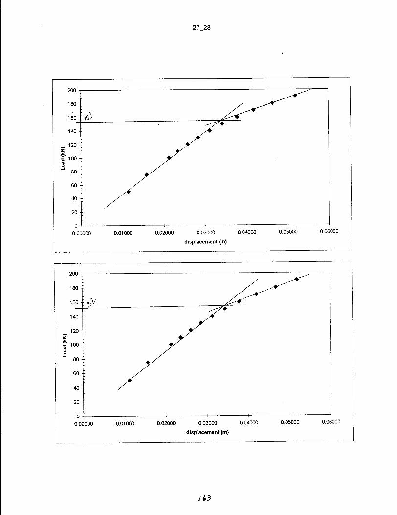
27_28

^

200 -r

180 -

160 -

140 -

_ 120 -z je u 100 • ra o

J 80-

•

60 -

40 - ' /

20 -

0 - 1— 1 —1 1 |

0.00000 0.01000 0.02000 0.03000 0.04000 0.05000 0.06000

displacement (m)

0.00000 0.01000 0.02000 0.03000 0.04000 0.05000 0.06000

displacement (m)

29 30

20 -'-

o i 1 1 1 -t— 1 0.00000 0.01000 0.02000 0.03000 0.04000 0.05000 0.06000

displacement (m)

200

60 f 40 -\

20 - :

0.00000 0.01000 0.02000 0.03000 0.04000 0.05000 0.06000 displacement (m)

31 32

3 3 3 4

Ib6

35 36

37 38

0.00000 0.01000 0.02000 0.03000 0.04000 0.05000 0.06000

displacement (m)

0.00000 0.01000 0.02000 0.03000 0.04000 0.05000 0.06000

displacement (m)

/68

39 40

Append ix E

170

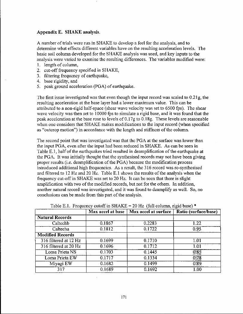
Appendix E . S H A K E analysis.

A number of trials were run in S H A K E to develop a feel for the analysis, and to determine what effects different variables have on the resulting acceleration levels. The basic soil column developed for the S H A K E analysis was used, and key inputs to the analysis were varied to examine the resulting differences. The variables modified were: 1. length of column, 2. cut-off frequency specified in S H A K E , 3. filtering frequency of earthquake, 4. base rigidity, and 5. peak ground acceleration (PGA) of earthquake.

The first issue investigated was that even though the input record was scaled to 0.2 lg , the resulting acceleration at the base layer had a lower maximum value. This can be attributed to a non-rigid half-space (shear wave velocity was set to 6500 fps). The shear wave velocity was then set to 10000 fps to simulate a rigid base, and it was found that the peak acceleration at the base rose to levels of 0.17g to 0.18g. These levels are reasonable when one considers that S H A K E makes modifications to the input record (when specified as "outcrop motion") in accordance with the length and stiffness of the column.

The second point that was investigated was that the PGA at the surface was lower than the input PGA, even after the input had been reduced in S H A K E . As can be seen in Table E. 1, half of the earthquakes tried resulted in deamplification of the earthquake at the PGA. It was initially thought that the synthesised records may not have been giving proper results (i.e. deamplification of the PGA) because the modification process introduced additional high frequencies. As a result, the 316 record was re-synthesised and filtered to 12 Hz and 20 Hz. Table E. 1 shows the results of the analysis when the frequency cut-off in S H A K E was set to 20 Hz. It can be seen that there is slight amplification with two of the modified records, but not for the others. In addition, another natural record was investigated, and it was found to deamplify as well. So, no conclusions can be made from this part of the analysis.

Table E. 1. Frequency cutoff in S H A K E = 20 Hz (full column, rigid base) * Max accel at base Max accel at surface Ratio (surface/base)

Natural Records Caltechb 0.1867 0.2283 1.22 Caltecha 0.1812 0.1722 0.95

Modified Records 316 filtered at 12 Hz 0.1699 0.1710 1.01 316 filtered at 20 Hz 0.1696 0.1712 1.01

Loma Prieta NS 0.1703 0.1445 0.85 Loma Prieta EW 0.1717 0.1334 0 78

Miyagi EW 0.1682 0.1499 0.89 317 0.1689 0.1692 1.00

171

The next trial was to reduce the cut-off frequency in S H A K E to 12 Hz, to see i f S H A K E was losing some of the peak input accelerations. The results of these runs are shown in Table E.2. Interestingly enough, the maximum acceleration at the base of the S H A K E column reduced even further from the scaled peak of 0.2lg. This suggests that some of the peak information is at frequencies above 12 Hz. However, the record that was filtered at 12 Hz before being put into S H A K E also experienced this decrease in P G A at the base, very curious. Also interesting, though, is that all records now see amplification at the surface. This shows that a long, soft column will tend to experience deamplification. Byrne et al. (1998) show a figure of acceleration on soft soil sites vs. rock sites, and it contains points that indicate deamplification. Although Idriss' (1990) median relationship does not account for this type of result, data points from a BC Hydro study and from a U B C study lie in the zone where acceleration on the soft soil is lower than on the rock site.

Table E.2. Frequency cutoff in S H A K E = 12 Hz (full column, rigid base) Max accel at base Max accel at surface Ratio (surface/base)

Caltechb (natural) 0.176 0.223 1.26 Caltechb (rigid base) 0.188 0.228 1.21

316 original 0.146 0.171 1.17 316 filtered at 12 Hz 0.147 0.171 1.17 316 filtered at 20 Hz 0.146 0.171 1.17

The next variable to be investigated was that of column length. It was suspected that the shorter the column, the higher the base input PGA. This suspicion was correct (if you compare the base accelerations of Table E.3a and b with Table E. l ) , but there was still a deamplification for some of the records.

Table E.3a. Short column (10 m) with rigid base.* Max accel at base Max accel at surface Ratio (surface/base)

Natural Records Caltechb 0.211 0.214 1.01 Caltecha 0.211 0.232 1.10

Modified Records 316 filtered at 12 Hz 0.211 0.197 0.94 316 filtered at 20 Hz 0.210 0.198 0.94

Lorna prieta NS 0.207 0.214 1.04 Lorna prieta E W 0.207 0.241 1.16

Miyagi E W 0.208 0.2063 0.99 317 (Caltecha mod) 0.2080 0.202 0.97

172

Table E.3b. Medium column (85 m) with rigid base * Max accel at

base Max accel at surface Ratio (surface/base)

Caltechb 0.192 0.224 1.16 Caltecha 0.189 0.179 0.95

316 original 0.190 0.172 0.91 316 filtered at 12 Hz 0.190 0.172 0.91 316 filtered at 20 Hz 0.190 0.172 0.91

The only trial that resulted in reasonable representation of the input PGA at the base, as well as expected amplification was the one in which the acceleration records were scaled to 0.1 g (Table E.4) The lower energy records do not induce as much damping in the column, and so the energy is not dissipated as the wave propagates through the column.

Table E.4 Full column with all input records scaled to O.lg* Max base accel Max surface accel Ratio (surface/base)

Natural Records Caltechb 0.0822 0.164 1.99 Caltecha 0.0790 0.134 1.70

Modified Records 316 original 0.0799 0.137 1.72

Loma Prieta NS 0.0794 0.120 1.51 Lorna Prieta E W 0.0827 0.0857 1.04

Miyagi E W 0.0750 0.115 1.54 317 0.0791 0.152 1.92

As a last check on the validity of the analysis results, it was decided to put the earthquakes through a S H A K E column (of the same site) developed by a colleague (personal communication, Singh, N . 1999). This column showed the same kind of response as the one under investigation and the deamplification was even more pronounced (Table E.5). This helps one to come to the conclusion that the P G A will decrease through a soil column of this length and softness.

Table E.5. Results from another version of the S H A K E column for the same site.* Neil's Column Max base accel Max surface accel Ratio (surface/base)

Caltechb 0.180 0.179 0.99 Caltecha 0.183 0.125 0.68

316 0.181 0.125 0.69 317 0.177 0.126 0.72

*Notes on tables: Rigid base -> Vs = 10000 fps Short column = 10 m Medium column = 85 m Full column = 240 m

173

The following conclusions were determined from this investigation: 1) The more rigid the base, the higher the input PGA 2) The shorter the column, the higher the input PGA 3) The lower the frequency cut-off in SHAKE, the higher the amplification of the PGA,

but the lower the value of input PGA 4) The lower the PGA (i.e. records scaled to 0.1 g as opposed to 0.2 lg), the higher the

amplification of the PGA. 5) More detailed columns (i.e. Neil's) do not give amplification for any of the

earthquakes tried, but give similar results to the author's column. 6) Amplification or deamplification is not a function of the type of earthquake record

used; deamplification was seen with both natural records, and synthesised records. 7) The apparent deamplification was only at the PGA, and the accelerations were

amplified at the first few (i.e. the significant) natural periods. The largest amplification was seen at the first natural period of the soil column (2.6 seconds). The results are thought to be due to the properties of the soil column itself - namely its length and softness. Some records show an amplification of the PGA (i.e. half of those tested), and some didn't, although the column remained the same for all runs.

174

Time Histories of Earthquakes used in SHAKE analysis (input earthquakes)

Loma Prieta NS modified to Van UHRS "99 0.3 -.-

0.2 -

- 0 . 1 o V „ re 0 _0) 8-0.1 -I u <

-0.2

-0.3 —i— 35 10 15 20 25

T ime ( s e c o n d s )

30 40

175

Miyagi EW Modified to Van UHRS '99

0.2 -

o w o -o 0) o -0.1 -o <

-0.2 -

-0 3

m 0.2 -

o w o -o 0) o -0.1 -o <

-0.2 -

-0 3 (

i i i i i i i ) 5 10 15 20 25 30 35 40

T ime ( s e c o n d s )

317 Modified to Van UHRS '99 0.3

0.2. I

-I 1 1 1 1 — : 1 1 1 1 0 5 10 15 20 25 30 35 40

T ime ( s e c o n d s )

176

Time Histories of Earthquakes after run through SHAKE column

Lorna Prieta NS after SHAKE

0.3

0.2 -

-| , , , , , , , 1 0 5 10 15 20 25 30 35 40

Time (seconds)

Lorna Prieta EW after SHAKE

H 1 1 1 1 1 1 1 1 0 5 10 15 20 25 30 35 40

Time (seconds)

177

Miyagi EW after SHAKE

317 after SHAKE

178

Appendix F

179

SAMPLE OF SHAKE INPUT FILE

Option 1 - Dynamic Soil Properties Set No. 1 1 3 9 G/Gmax for Clay (Idriss 1990)

0. 0001 0.0003 0.001 0.003 0.01 0.03 0.1 0.3 1. 1. 1. 1. 0.981 0.941 0.847 0.656 0.438 0.238

9 Damping for Clay (Idriss 1990) 0.0001 0.0003 0.001 0.003 0.01 0.03 0.1 0.3

0.24 0.42 0.8 1.4 2.8 5.1 9.8 15.5 21.

9 G/Gmax for Sand (Idriss 1990) 0. 0001 0.0003 0.001 0.003 0.01 0.03 0.1 0.3 1. 1. 1. 0.99 0.96 0.85 0.64 0.37 0.18 0.08

9 Damping for Sand (Idriss 1990) 0.0001 0.0003 0.001 0.003 0.01 0.03 0.1 0.3

0.24 0.42 0.8 1.4 2.8 5.1 9.8 15.5

16 G/Gmax for Ti l l (Murphy 1978) 0.0001 0.0002 0.0005 0.001 0.002 0.005 0.01 0.02 0. 05 0.1 0.2 0.5 1. 2. 5. 10. 1. 1. 0.987 0.939 0.894 0.79 0.664 0.531 0.347 0.24 0.17 0.088 0.049 0.03 0.025 0.02

16 Damping for Ti l l (Murphy 1978) 0.0001 0.0002 0.0005 0.001 0.002 0.005 0.01 0.02 0.05 0.1 0.2 0.5 1. 2. 5. 10. 0. 0. 0.15 0.9 1.65 3.15 5.1 7.05 9.75 11.4 12.45 13.65 14.25 14.55 14.7 14.7

3 1 2 3 Option 2 - Soil Profile Set No. 1

1.

1.

21.

2 1 43 based on FD94-4 1 2 8.2 0.05 2 1 6.56 0.05 3 2 4.921 0.05 4 2 4.921 0.05 5 2 6.562 0.05 6 2 6.562 0.05 7 2 6.562 0.05 8 2 6.562 0.05 9 2 6.562 0.05 10 2 6.562 0.05 11 2 6.562 0.05 12 2 6.562 0.05 13 2 8.202 0.05 14 2 6.562 0.05 15 2 6.562 0.05 16 2 6.562 0.05 17 2 6.562 0.05 18 2 6.562 0.05 19 2 6.562 0.05 20 2 8.202 0.05 21 2 8.202 0.05 22 2 6.562 0.05 23 2 6.562 0.05 24 2 9.842 0.05 25 2 32.808 0.05 26 2 32.808 0.05 27 1 32.808 0.05 28 1 32.808 0.05 29 1 32.808 0.05 30 1 32.808 0.05 31 1 32.808 0.05

0.121 410.0 0.121 410.0 0.121 410.0 0.121 410.0 0.1241 410.0 0.1241 410.0 0.1241 410.0 0.1241 410.0 0.1241 492.0 0.1241 492.0 0.1241 492.0 0.1241 558.0 0.1241 558.0 0.121 656.0 0.121 656.0 0.121 656.0 0.121 738.0 0.1241 738.0 0.1241 738.0 0.1241 820.0 0.121 820.0 0.121 820.0 0.121 820.0 0.1241 820.0 0.1241 984.0 0.1241 984.0 0.1305 984.0 0.1305 1066.0 0.1305 1148.0 0.1305 1230.0 0.1305 1230.0

180

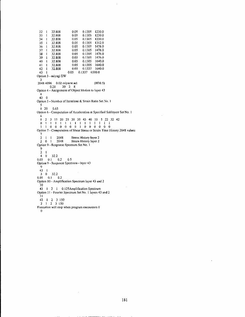
32 1 32.808 0.05 0.1305 1230.0 33 1 32.808 0.05 0.1305 1230.0 34 1 32.808 0.05 0.1305 1230.0 35 1 32.808 0.05 0.1305 1312.0 36 1 32.808 0.05 0.1305 1476.0 37 1 32.808 0.05 0.1305 1476.0 38 1 32.808 0.05 0.1305 1476.0 39 1 32.808 0.05 0.1305 1476.0 40 1 32.808 0.05 0.1305 1640.0 41 1 32.808 0.05 0.1305 1640.0 42 1 32.808 0.05 0.1337 1640.0 43 1 0.05 0.1337 6500.0

Option 3 3

- miyagi E W

2048 4096 0.02 miyaew.acl (8fl0.5) 0.21 20 2 8

Option 4 - Assignment of Object Motion to layer 43 4

43 0 Option 5 - Number of Iterations & Strain Ratio Set No. 1

5 1 20 0.65

Option 6 - Computation of Acceleration at Specified Sublayers Set No. 1 6 1 2 3 15 20 25 30 35 43 40 10 5 22 32 42 0 1 1 1 1 1 1 1 1 1 1 1 1 1 1 1 1 0 0 0 0 0 0 1 0 0 0 0 0 0

Option 7 - Computation of Shear Stress or Strain Time History 2048 values 7 2 1 1 2048 Stress History layer 2 2 0 1 2048 Strain History layer 2

Option 9 - Response Spectrum Set No. 1 9 2 1 4 0 32.2

0.05 0.1 0.2 0.5 Option 9 - Response Spectrum - layer 43

9 43 1 3 0 32.2

0.05 0.1 0.2 Option 10 - Amplification Spectrum layer 43 and 2

10 43 1 2 1 0.125Amplification Spectrum

Option 11 - Fourier Spectrum Set No. 1 layers 43 and 2 11 43 1 2 3 150 2 1 2 3 150

Execution will stop when program encounters 0 0

181

ShakEdit No5_28.EDT FILE (database file)

Option 1 - Dynamic Soil Properties Set No. 1 1 3 9 G/Gmax for Clay (Idriss 1990)

0. 0001 0.0003 0.001 0.003 0.01 0.03 0.1 0.3 1. 1. 1. 1. 0.981 0.941 0.847 0.656 0.438 0.238

9 Damping for Clay (Idriss 1990) 0.0001 0.0003 0.001 0.003 0.01 0.03 0.1 0.3 1. 0.24 0.42 0.8 1.4 2.8 5.1 9.8 15.5 21.

9 G/Gmax for Sand (Idriss 1990) 0. 0001 0.0003 0.001 0.003 0.01 0.03 0.1 0.3 1. 1. 1. 0.99 0.96 0.85 0.64 0.37 0.18 0.08

9 Damping for Sand (Idriss 1990) 0.0001 0.0003 0.001 0.003 0.01 0.03 0.1 0.3 1. 0.24 0.42 0.8 1.4 2.8 5.1 9.8 15.5 21.

16 G/Gmax for Til l (Murphy 1978) 0.0001 0.0002 0.0005 0.001 0.002 0.005 0.01 0.02 0. 05 0.1 0.2 0.5 1. 2. 5. 10. 1. 1. 0.987 0.939 0.894 0.79 0.664 0.531 0.347 0.24 0.17 0.088 0.049 0.03 0.025 0.02

16 Damping for Ti l l (Murphy 1978) 0.0001 0.0002 0.0005 0.001 0.002 0.005 0.01 0.02 0.05 0.1 0.2 0.5 1. 2. 5. 10. 0. 0. 0.15 0.9 1.65 3.15 5.1 7.05 9.75 11.4 12.45 13.65 14.25 14.55 14.7 14.7

3 1 2 3 Option 2 - Soil Profile Set No. 1

2 1 43 based on FD94-4 1 2 8.2 0.05 2 1 6.56 0.05 3 2 4.921 0.05 4 2 4.921 0.05 5 2 6.562 0.05 6 2 6.562 0.05 7 2 6.562 0.05 8 2 6.562 0.05 9 2 6.562 0.05 10 2 6.562 0.05 11 2 6.562 0.05 12 2 6.562 0.05 13 2 8.202 0.05 14 2 6.562 0.05 15 2 6.562 0.05 16 2 6.562 0.05 17 2 6.562 0.05 18 2 6.562 0.05 19 2 6.562 0.05 20 2 8.202 0.05 21 2 8.202 0.05 22 2 6.562 0.05 23 2 6.562 0.05 24 2 9.842 0.05 25 2 32.808 0.05 26 2 32.808 0.05 27 1 32.808 0.05 28 1 32.808 0.05 29 1 32.808 0.05 30 1 32.808 0.05 31 1 32.808 0.05

0.121 410.0 0.121 410.0 0.121 410.0 0.121 410.0 0.1241 410.0 0.1241 410.0 0.1241 410.0 0.1241 410.0 0.1241 492.0 0.1241 492.0 0.1241 492.0 0.1241 558.0 0.1241 558.0 0.121 656.0 0.121 656.0 0.121 656.0 0.121 738.0 0.1241 738.0 0.1241 738.0 0.1241 820.0 0.121 820.0 0.121 820.0 0.121 820.0 0.1241 820.0 0.1241 984.0 0.1241 984.0 0.1305 984.0 0.1305 1066.0 0.1305 1148.0 0.1305 1230.0 0.1305 1230.0

182

32 1 32.808 0.05 0.1305 1230.0 33 1 32.808 0.05 0.1305 1230.0 34 1 32.808 0.05 0.1305 1230.0 35 1 32.808 0.05 0.1305 1312.0 36 1 32.808 0.05 0.1305 1476.0 37 1 32.808 0.05 0.1305 1476.0 38 1 32.808 0.05 0.1305 1476.0 39 1 32.808 0.05 0.1305 1476.0 40 1 32.808 0.05 0.1305 1640.0 41 1 32.808 0.05 0.1305 1640.0 42 1 32.808 0.05 0.1337 1640.0 43 1 0.05 0.1337 10000.0

Option 3 3

- caltecha.acl

(8fl0.0) 3800 4096 0.02 caltecha.acl 2.4004E-04 20 28 8 Option 3 - caltechb

3 3800 4096 0.02 caltechb.acl 1.1356E-04 20 29 8 Option 3 - orig 316 cm/s

3 3800 4096 0.02 316_or.acl 0.001019 20 1 8

Option 3 - loma prieta NS 3

2048 4096 0.02 lpns.acl 0.21 20 2 8

Option 3 - loma prieta EW 3

2048 4096 0.02 Ipew.acl 0.21 20 2 8

Option 3 - miyagi E W 3

2048 4096 0.02 miyaew.acl 0.21 20 2 8

Option 3 - 317 modified 3

2048 4096 0.02 317mod.acl 0.21 20 2 8 - Assignment of Object Motion to layer 43

(8fl0.0)

(8f 10.3)

(8H0.5)

(8A0.5)

(8fl0.5)

(8H0.5)

Option 4 • 4

43 0 Option 5 •

5 1 20

Number of Iterations & Strain Ratio Set No. 1

0.65 Option 5 - Number of Iterations & Strain Ratio for equake 3

5 0.65 Computation of Acceleration at Specified Sublayers Set No.

10 Option 6

6 1 2 0 1 1 1

42 3 15 20 25 30 35 43 40 10 5 22 32 1 1 1 1 1 1 1 1 1 1 1 1 1 0 0 0 0 0 0 1 0 0 0 0 0 0

Option 7 - Computation of Shear Stress or Strain Time History 2048 values 7

1 2048 Stress History layer 2 1 2048 Strain History layer 2

- Computation of Shear Stress or Strain Time History 4096 values

2 1 2 0

Option 7 7 2 1 1 2 0 1

Option 9 9 2 1 4 0

0.05 0.1 0.2 0.5 Option 9 - Response Spectrum - layer 43

9 43 1

3800 Stress History layer 2 3800 Strain History layer 2

Response Spectrum Set No. 1

32.2

183

3 0 32.2 0.05 0.1 0.2 Option 9 - Response Spectrum Set No. 3

9 20 1 3 0 32.2

0.05 0.1 0.2 Option 10 - Amplification Spectrum layer 43 and 2

10 43 1 2 1 0.125Amplification Spectrum

Option 11 - Fourier Spectrum Set No. 1 layers 43 and 2 11 43 1 2 3 150 2 1 2 3 150

Execution will stop when program encounters 0 0

FLAC DYNAMIC INPUT FILE ;fric30.dat

; No. 5 Rd Bridge ; free field used ; units kN-m ; mesh 300X300 in abutment zone ; top of abutment is structural element ; Apri l 1999 ; Georgia Lysay ; sensitivity on friction angle - gamma and dens set to ; four values of fric 30, 33, 36, and 39 deg

config ex 1 dynamic

FISH FUNCTIONS

IsAbutment

returns true (1) if given i j point is in abutment and false (0) i f not

In the defined grid there are two regular rectangles that make up the abutment. They are first one: i =46 to 61, j = 9 to 12 second one: i = 48 to 57, j = 13 to 21

define IsAbutment ; point is not abutment by default

IsAbutment = 0

; first rectangle: i = 24 to 31, j = 14 to 15

i f i>=24 i f i<=31 i f j>= 14 i f j<=15

IsAbutment = 1 exit

endif endif

endif endif

; second rectangle: i = 25 to 29, j = 16 to 20

i f i >=25 i f i<=29

ifj >= 16 if j <= 20

IsAbutment = 1 exit

endif endif

endif endif

end

SetAbutmentProps

define SetAbutmentProps shearmod(i j ) = 1E4 ; this should be higher - at 11.2e6 bu lkmod( i j ) = 1E4 ; this should be higher, too - at 18.7e6 density(ij) =2.5 friction(ij) =45 cohesion(ij) = 1000

end

GenRandSeed

define GenRandSeed randSeed = 11 loop n (1,randSeed)

dummy = grand endloop

end

SetSoilProps

define SetSoilProps mean = 12 ; N160 is defined as a normal random stddev = 3 ; variable with the given mean and n l_60 = stddev * grand + mean ; standard deviation i f n l_60<0 .0

command print nl_60

endcommand nl_60=mean

endif atm = 100.0 ; atmospheric pressure (kPa)

mean_stress = abs(((syy(i j ) + sxx(i j ) + szz(i j))/3)) meanstress = max(mean_stress, 0.02 * atm) ex_l(ij)=mean_stress gmax = 440.0 * (nl_60A0.333333) * atm * sqrt(mean_stress/atm)

sfactor = 0.5 bfactor = 0.27

shear_mod(i j ) = sfactor * gmax bulk_mod(i j ) = bfactor * gmax

cohesion(ij) =2

end

SetDynSoilProps

define SetDynSoilProps mean = 23 ; N160 is defined as a normal random ;stddev = 3 ; variable with the given mean and ;nl_60 = stddev * grand + mean ; standard deviation nl_60 = mean ; set nl-60 to mean over entire structure i f n l_60<0 .0

command print nl_60

endcommand nl 60=mean

186

endif atm= 100.0 ; atmospheric pressure (kPa)

mean_stress = abs(((syy(i j ) + sxx(i j ) + szz(i j))/3)) mean_stress = max(mean_stress, 0.02 * atm) ex_l(ij)=mean_stress gmax = 440.0 * (nl_60A0.333333) * atm * sqrt(mean_stress/atm)

sfactor = .14 ; check with S H A K E bfactor = 1 ; check with S H A K E

shear_mod(i j ) = sfactor * gmax bulk_mod(i j ) = bfactor * gmax

cohesion(ij) = 2

end

SetlnitialProps

set the initial properties for all i j points

define SetlnitialProps loop i ( l jzones)

loopj ( l jzones) if IsAbutment = 0

SetSoilProps else

SetAbutmentProps endif

endloop endloop

end

SetDynamicProps

sets the properties for dynamic analysis

define SetDynamicProps loop i ( l jzones)

loop j( l jzones) if IsAbutment = 0

SetDynSoilProps else

SetAbutmentProps endif

endloop endloop

end

F L A C C O M M A N D S

; set up grid

grid 55,26 model mohr

initial x = 0.00 i= 1 initial x = 0.50 i= 2

187

initial initial initial initial initial initial initial initial initial initial initial initial initial initial initial initial initial initial initial initial initial initial initial initial initial initial initial initial initial initial initial initial initial initial initial initial initial initial initial initial initial initial initial initial initial initial initial initial initial initial initial initial initial initial

x = x = x = X =

X =

X =

X =

X =

X =

X =

X =

X =

X =

X =

X =

X =

X =

X =

X =

X =

X =

X =

X =

X =

X =

X =

X =

X =

X =

X =

X =

X =

X =

X =

X =

X =

X =

X =

X =

X =

X =

X =

X =

X =

X =

X =

X =

X =

X =

X =

X =

X =

X =

X =

1.00 I. 50 2.00 2.50 3.00 3.50 4.00 4.50 5.00 5.50 6.00 6.51 6.96 7.37 7.74 8.07 8.40 8.70 9.00 9.30 9.60 9.90 10.20 10.50 10.80 II. 10 11.40 11.70 12.00 12.30 12.60 12.90 13.20 13.50 13.84 14.21 14.63 15.11 15.61 16.11 16.61 17.11 17.61 18.11 18.61 19.11 19.61 20.11 20.61 21.11 21.61 22.11 22.61 23.11

initial initial initial initial initial initial initial initial initial initial initial initial initial initial

0.00 0.68 1.36 2.00 2.65 3.19 3.67 4.11 4.51 4.87 5.20 5.50 5.80 6.10

initial y = 6.40 j = 15 initial y = 6.70 j = 16 initial y = 7.00 j = 17 initial y = 7.30 j = 18 initial y = 7.60 j = 19 initial y = 7.90 j = 20 initial y = 8.20 j = 21 initial y = 8.50 j = 22 initial y = 8.80 j = 23 initial y = 9.10 j = 24 initial y = 9.40 j = 25 initial y = 9.70 j = 26 initial y = 10.00 j = 27

gen line 0.0,2.0 gen line 8.4,7.6 gen line 10.2,7.6 gen line 10.2,8.2 gen line 11.7,8.2

8.4,7.6 10.2,7.6 10.2,8.2 11.7,8.2 11.7,10.0

model null region 1,6

; put i n structural elements to model the top of the abutment struct prop 1 area 0.3 density 2.5 e 28000000 i .00225 pmom 900

struct beam begin grid=30,21 end grid=30,22 vertical beams struct beam begin grid=30,22 end grid=30,23 struct beam begin grid=30,23 end grid=30,24 struct beam begin grid=30,24 end grid=30,25 struct beam begin grid=30,25 end grid=30,26 struct beam begin grid=30,26 end grid=30,27

struct beam begin grid=25,21 end grid=26,21 struct beam begin grid=26,21 end grid=27,21 struct beam begin grid=27,21 end grid=28,21 struct beam begin grid=28,21 end grid=29,21 struct beam begin grid=29,21 end grid=30,21

fix x i=56 fix x,y j=l fix x i=l j=l,4

;horizontal beams ; on abutment

• check properties - take out top row of elements

;pause

GenRandSeed set ncwrite 100

; turn on gravity set dyn=off set gravity=9.81

; set mean values of friction and density prop fric 30 density 1.9

; set initial properties to generate stresses prop shear 10000 bulk 10000 coh 500 step 1000

;pause

; set properties according to random (N 1)60 SetlnitialProps

; apply dead load to abutment

apply yforce =-62 i=28 j=21 step 1000

ini ydisp=0.0 xdisp=0.0

189

; set the dynamic properties SetDynamicProps

; apply dynamic load set multi on

set dyn=on apply ff ;free field boundary applied set dy_damp=rayleigh .08 2.0 ;from comparison with F L A C col and S H A K E set dytime=0.0

;his read 100 flacl.acl ; E A R T H Q U A K E flac*.acl in g - Dr Anderson's record. ;apply xacc = 9.81 hist 100 j=l ;multiply by gravity to get into m/s/s ;apply yacc =0.0 j=l

;his read 100 calb_fl.acl ;natural caltech record from Dr. Byrne in cm/s/s*10 ;apply xacc = 0.00111405 hist 100 j=l jmultiply get into m/s/s and scaled to 0.21 g

his read 100 calshake.acl ; record from S H A K E in g apply xacc = 9.81 hist 100 j=l ; multiply to get into m/s/s apply yacc =0.0 j=l

;apply xacc = 9.81 hist 100 i=56 ; use these when not using free field ;apply yacc = 0.0 i=56 ;apply xacc = 9.81 hist 100 i=l j=l,3 ; use these when not using free field ;apply yacc = 0.0 i= 1 j= 1,3

; histories hist dytime his xvel i=27 j=l his xvel i=27 j=7 his xvel i=27 j=14 his xdisp i=27j=l hisxdisp i=27j=7 his xdisp i=27j=14 his xacc i=27 j=l his xacc i=27 j=7 his xacc i=27 j=14 hist ydis i=30 j=27 his xdisp i=28 j=21 his ydisp i=28 j=21 hist ydis i=27 j=l hist ydis i=27 j=7 hist ydis i=27 j=14 hist syy i=27 j=14 hist unbal hist shear mod

;base ;mid height (or so) ;bottom of abutment

;top of abutment ;plateau of abutment

;bottom of abutment

step 10000

step 700000

def ResetXDisp ; corrects displacements induced by no baseline correction on record loop i (l,izones+l)

loop j (2jzones+l) xdisp(i j ) = xdisp(ij)-xdisp(i,l)

endloop endloop loop i (l,izones+l)

xdisp(i,l) = 0.0 endloop end

ResetXDisp

save fric30b.sav

190

ShakEdit GRF File No of Analyses: ShakEdit Flags:

1 1

Soil Profile Identification based on FD94-4

Soil Deposit Number:1 Period for Soil Column 3.07 sec Average Shear Wave Velocity for Soil Column 985 ft/sec

Analysis No. 1 Earthquake MIYAEW.ACL

No. of Soil Layers 43 No. of Peak Acceleration Values 15

Layer Depth Unit Damping Shear

Weight Modulus

(ft) (kef) (%) (ksf)

1 4.1 0.121 2.7 543.7

2 11.48 0.121 4.7 545.8

3 17.22 0.121 8.4 284.9

4 22.14 0.121 10.4 220.4

5 27.88 0.124 12.5 182

6 34.44 0.124 16 110.7

7 41.01 0.124 17.4 94.3

8 47.57 0.124 18.6 80.6

9 54.13 0.124 15.1 179

10 60.69 0.124 16.2 155.5

11 67.25 0.124 16.9 144.3

12 73.82 0.124 14 276.5

13 81.2 0.124 15.6 214.8

14 88.58 0.121 11.4 514.3

15 95.14 0.121 11.8 490.3

16 101.7 0.121 12.2 468

17 108.27 0.121 10 746.2

18 114.83 0.124 10 764.6

19 121.39 0.124 10.2 748.8

20 128.77 0.124 8.5 1149.2

21 136.97 0.121 8.900001 1068.6

22 144.36 0.121 9.2 1029

23 150.92 0.121 9.5 971.3

24 159.12 0.124 9.8 955.5

25 180.45 0.124 7.900001 1796.4

26 213.25 0.124 9 1552.5

27 246.06 0.131 6.6 3084.5

28 278.87 0.131 ' 6.1 3709.2

29 311.68 0.131 5.7 4402.6

30 344.49 0.131 5.3 5151.1

31 377.29 0.131 5.5 5085.3

32 410.1 0.131 5.8 5019.8

33 442.91 0.131 6 4976.4

34 475.72 0.131 6.2 4917.4

35 508.53 0.131 5.8 5697.4

36 541.33 0.131 5 7500.4

37 574.14 0.131 5.2 7453.4

38 606.95 0.131 5.3 7394.3

39 639.76 0.131 5.5 7347.2

40 672.57 0.131 4.8 9352.7

41 705.37 0.131 4.9 9334.7

42 738.18 0.134 4.8 9579.6

43 Base

Max Max Shear Depth Max

Strain Stress Wave Vel. Max Acc Acc

(%) (psf) (fps) (ft) (9) 0.01368 74.37 380.3776 0 0.14994

0.03779 206.26 381.1115 8.2 0.14683

0.10723 305.45 275.3477 14.8 0.14052

0.1738 383.04 242.1815 — — 0.25759 468.7 217.3966 24.6 0.12905

0.51542 570.45 169.5473 — — 0.6988 658.98 156.4851 — —

0.90131 726.62 144.672 — — 0.43337 775.77 215.5974 — — 0.5418 842.48 200.9474 57.4 0.14266

0.62558 902.98 193.5754 — — 0.34464 953 267.9567 — — 0.46739 1003.76 236.1752 — — 0.20762 1067.86 369.9504 — — 0.22622 1109.18 361.2153 91.9 0.12075

0.24501 1146.52 352.9053 — — 0.15864 1183.84 445.6182 — — 0.15896 1215.45 445.5888 — — 0.16604 1243.29 440.9608 — — 0.1108 1273.37 546.2795 124.7 0.10924

0.12141 1297.46 533.2647 — — 0.13034 1341.14 523.2906 141.1 0.10309

0.14432 1401.75 508.4075 — — 0.15504 1481.34 498.1182 — — 0.09363 1681.88 682.9967 164 0.1046

0.12529 1945.16 634.9403 — — 0.06779 2090.84 870.7324 — — 0.05999 2225.2 954.844 — — 0.05326 2344.82 1040.272 — — 0.0482 2482.85 1125.233 328.1 0.10084

0.05157 2622.66 1118.023 — — 0.05517 2769.31 1110.799 393.7 0.11539

0.05769 2870.8 1105.987 — — 0.0613 3014.14 1099.411 — —

0.05588 3183.52 1183.397 492.1 0.12362

0.04483 3362.68 1357.796 — — 0.04699 3502.3 1353.535 — — 0.04901 3624.29 1348.158 — — 0.05069 3724.4 1343.858 — — 0.04058 3795.41 1516.215 656.2 0.1576

0.04137 3861.92 1514.755 — — 0.04068 3897.1 1517.222 721.8 0.17007

754.6 0.1682

I9I

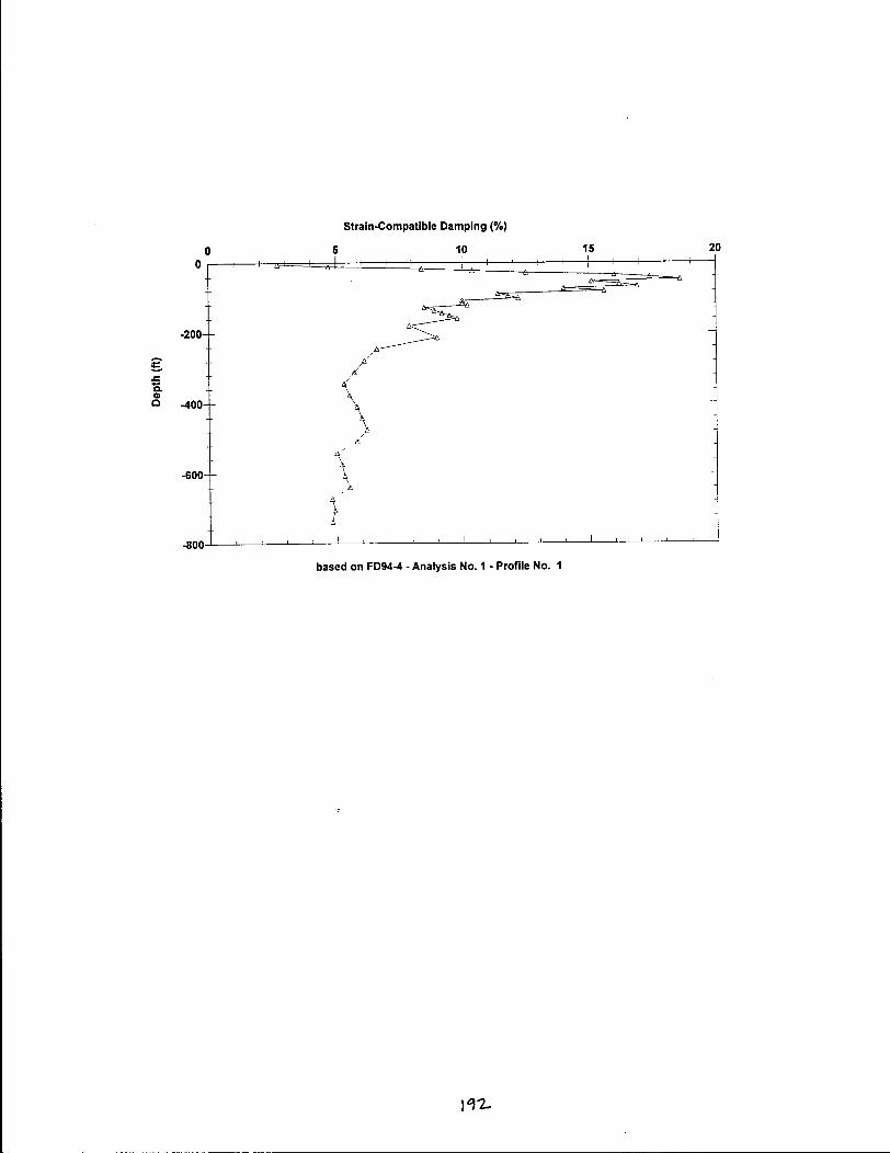
Strain-Compatible Damping (%)

-200+

-400+ \

based on FD94-4 - Analysis No. 1 - Profile No. 1

Strain-Compatible Shear Modulus (ksf)

Maximum Shear Strain (%)

0.0 0.2 0.4 0.6 0.8 0 |JR_4 L , 1 '.I 1 1 1 1 I ' 1 1 1 1 1 1 1 ' H

based on FD94-4 • Analysis No. 1 - Profile No. 1

Maximum Shear Stress (psf)

0 1000 2000 3000 4000

. 8 0 0 J , , , : 1 : . . 1 1 . • ' '

based on FD94-4 - Analysis No. 1 - Profile No. 1

115

Shear Wave Velocity (fps)

Peak Acceleration (g)

based on FD94-4 - Analysis No. 1 - Profile No. 1

in

Appendix G

198

Soi l Properties Survey

The following questionnaire involves questions about basic soil properties. The test case is an abutment structure founded on an embankment constructed from Fraser River Sand. The fill is 10 m in height with sideslopes of 1.5H:1V, and is to be compacted to a cone tip resistance (q e) of 10 Mpa or ( N , ^ = 20. The sand is unsaturated.

The results of the questionnaire will be used to develop probabilistic distributions of the friction angle and unit weight. The distributions will be used in a (probabilistic) finite difference analysis that will explore the effects of soil properties defined by random variables.

There are one or two questions for each soil property. Please answer the questions quickly, based on your instinct and experience, without applying safety factors or conservative estimates. Space has been provided on the questionnaire for your answers, as well as for any additional comments. The survey should take approximately 15 minutes to complete.

F r i c t i o n A n g l e

1. What is the mean friction angle of Fraser River Sand?

2. Please estimate the chance that the friction angle falls into the following ranges of values (in percentages adding up to 100%):

< 26°

26° - 30°

31° - 3 5 °

36° - 40°

> 4 0 °

S a t u r a t i o n

What is the likelihood that the average level of saturation in this type of embankment falls into the following ranges? Please estimate in percentages adding up to 100%:

0 - 25%

26 % - 50 %

51 % - 75 %

199

7 6 % - 1 0 0 %

Un i t W e i g h t

1. What is the mean unit weight of Fraser River Sand?

2. Please estimate the chance that the unit weight falls into the following ranges of values (in percentages adding up to 100%):

< 16 kN/m 3

16 kN/m 3 - 1 7 kN/m 3

18 kN/m 3 - 1 9 kN/m 3

20 kN/m 3 - 21 kN/m 3

22 kN/m 3 - 23 kN/m 3

> 23 kN/m 3

If an (N^so o f 2 0 i s specified for this site, what range in values would you realistically expect to get in the field for ( N , ^ ? Please estimate the chance that ( N ^ o falls into the following ranges of values (in percentages adding up to 100%):

< 10

1 0 - 1 5

1 6 - 2 0

2 1 - 2 5

26 - 30

> 30

C o m m e n t s

200

04/16/99 08:39 © 2 5 0 356 7798 HIGHWAY ENG.VIC. UBC CIVIL hMGlfsfc LflJUU^/UO?

Soil Properties Survey

The following questionnaire Involves questions about basic soil properties. The test case is an abutment structure founded on an embankment constructed from Fraser River Sand. The fill is 10 m in height with side slopes of 1.5H:1V, and is to be compacted to a cone tip resistance (qj af 10 Mpa or (N,)M = 20. The sand Is unsaturated.

The results of the questionnaire will be used to develop probabilistic distributions of thB friction angle and unit weight The distributions will be used in a (probabilistic) finite difference analysis that will explore the effects of soil properties defined by random variables.

There are on* or two questions for each soil property. Please answer the questions, based on your instinct and experience, without applying safety factors or conservative estimates. Space has been provided on the questionnaire for your answers, as well as for any additional comments.

" The survey should take approximately 15 minutes to completer-

Friction Angle

1. What is the mean friction angle of Fraser River Sand?

2. Please estimate the chance that tha friction angls falls into the following ranges of values (in percentages adding up to 100%):

<26" —^-26° - 30° — ! _ 31°-36" 36° - 40°

>40" 2 -loo

Saturation

What is the likelihood that the average level of saturation in this type of embankment falls Into the following ranges? Please estimate in percentages adding up to 100%:

1

0 - 25% - 3 — 26 % - 50 % 51%-75% —1£-76 % - 100 % _£i2-

too/coo® ASVMHilS 830103 CSZS 862 £09 T© S0:ST CS/ST/J'O

0 4 / 1 6 / 9 9 08 :39 ^ 2 5 0 358 77U8 HlblittAY. ENG.V IC . -»-»-» LUC C I V I L t ^ G i l N h IgJUOO/UO

Unit Weight

1. What is the mean unit weight of Fraser River Sand?

2. Please estimate the chance that the/unit weight falls into the following ranges of values (in percentages adding up to 100%):

< 16 kN/m* J O

1B kN/m 3 -17 kN/m 3 ^ <

J8kN /m 3 - l9kN /m a

20 kN/m 3 - 21 kN/m 3 S

22 kN/m 3 - 23 kN/m 3 O

> 23 kN/m 3 0

to*

60

If an (N,)es of 20 is specified for this site, what range in values would you realistically expect to get In the field for (N,)*,? Please estimate the chance that (N,)*, falls Into the following ranges of values (In percentages adding up to 100%):

< 10

10-15 2. 16-20

21-25 1° «F ffetlot . WJR* T>K»*^T^ .

26-30

>30 [tX9

Comments

roo/rooia AgVMHTtg H3CTI09 CSZS 86Z t09 TO 90 = 51 68/ST/tO

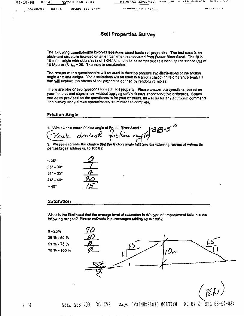
04 / 1 6 / 99 U » : 4 U '££250 35B 7/D5 tlUjtlTTAX t , I N t . . V l C . -»-»-•_ unv, 11 > I L C.IOII>C I^UUI/UU/

Sol! Properties Survey

The following questionnaire Involves questions about basic toll properties. The test case is an abutment structure roundad on an embankment constructed from Fraser River Sand. The fill is 10 m in height with side dopes of 1,6H: 1V, and is to ba compacted to a cone tip resistance (qj of 10 Mpa or (N,)« « 20. The sand is unsaturated.

Tha results of tha questionnaire will be used lo dovelop probabilistic distributions Df the friction angle and unit weight. The distributions will be used in a (probabilistic] finite dlffsrenca analysis that will explore the effects of soli properties defined by random variables,

There are one or two questions for each soil property. Please answer the questions, based on your instinct and experience, without applying safety factors or conservative estimates. Space has been provided on the questionnaire for your answers, as wen as for an/ additional comments. The survey should taka approximately 15 minutes to complete.

Friction Angle

1. What Is the mean friction angle of Fraser River Sand? 1 ^ 3 ^ ' ^ ^

^ T 6 . f c ckrtKcVaJl ^'CQTIA. Ctpff^

G y

2. Please estimate the chance that the friction angle fafls into the following ranges of values (in percentages adding up to 100%):

26*-30» / 31" -35° A 36" - 40° $Q >40'

Saturation

What is the likelihood that the average level of saturation in this type of embankment fails Into the following ranges7 Please estimate in percentages adding up to 100%:

0-25'/. 26 % • 50 % 51 %-7S% 76%-100%

7 'd SILL 586 709 "ON XV5 1 * 3 1V0INH0H10H0 aOHlOVW WJ flHX 66-SI -HaV

04/16/99 08:40 ® 2 5 0 356 7798

D j / 0 0 / 9 9 09 :58 « 2 E 0 338 77fl8

HIGHWAY ENG. VIC. -»-»-» U B C C I V I L fclNGilSt l g J U U 5 / U U 7

HIGHWAY •*""" '

Unit Weight

1. what is the mean unit weight of Fraser River Sand?

2. Please estimate the chance that the unit weight bill Into the fallowing ranges of values (in percentaBcs adding up to 100%):

16 kN/m'/lfW 1 1 .N/m'

2fi cN/ms

18 kN/m'

20kNVm' 22kN/mf-2^kN/m4

> 23 kNrW

_£1

if a n CN \ of 20 Is specified for this site, what range in values would you realistically expect to get InlSifield fer (N, J PlSse «timate the ehanJtf . i t (N,)K falls into the ftMne ran8es of values (in percentages adding up to 100%):

<10 10-15 16-20 21 -25 26 '30 >30

4-JL

ML

C o m m e n t s

S 'd 96Z.Z. 986 >09 'ON XV i loH 1VOINH03XOHO a031DVW Hd 5T.6 fiHi

0 4 / 1 6 / 9 9 0 8 : 4 0 © 2 5 0 356 7798 HIGHWAY ENG . V I C . -»-»-> UBC C I V I L £.INOI:N£. i fcjuuo/uuy

Q 3 / 3 0 / 9 8 08 :35 ' Q ' 2 5 0 359 77Wtf m w i i i i j o i n , . ! ^

Soil Properties Survey

The fallowing questionnaire involves questions about basic soil properties. The last cats is an abutment structure founded on an embankment constructed from Fraser River Sand. The fill Is 10 m in height with side slopes of 1.6H:1V, and is to be compacted to a cone tip resistance (qj of 10 Mpa or (N,)6B

a 20. The 6and Is unsaturated,

The results of the questionnaire will be used to develop probabilistic distributions of the friction angle and unit weight. The-dlslrlbulions will be used In a (probabilistic) finite difference analysis that will explore tha effects of soil properties defined by random variables.

There aro one or two questions (or each soil property. Please answer the questions, based on your Instinct and experience, without applying safety factors or conservative estimates. Space has been provided on tha questionnaire for your answers, as wall as for any additional comments. The survey should take approximately 15 minutes to complete.

Friction Angle

1. vVhat Is the mean friction angle of Fraser River Sand? . . r <d> 1 - S 2 ~ [ 3 i ° - 3 S ° J U v ^ ^ r f l v n M jS*»eci<iM ' L ^ T S A J

2. Please estimate the chance that the friction angle falls into ths following ranges of values {In percentages adding up to 100%):

< 2 6 *

2 6 ' - 3 0 »

31e-35" 36* -40°

Satura t ion

J2 g o

4>. or

Tea V -fcich'O" Qr^'

What Is the likelihood that the average level of saturation In thU type of embankment fella Into the following ranges? Please estimate in percentages adding up to 100%;

0-25*/. 2 6 % - 5 0 %

5 1 % - 7 5 %

7 6 % - 1 0 0 %

5 2 U S96 v09 'ON XVJ 1V01NH03I0HO A0313VH 6v:Z AH1 66-91-HdV