comparison of high order algorithms in aerosol and … · comparison of high order algorithms in...

HAL Id: hal-00917411https://hal.inria.fr/hal-00917411

Submitted on 11 Dec 2013

HAL is a multi-disciplinary open accessarchive for the deposit and dissemination of sci-entific research documents, whether they are pub-lished or not. The documents may come fromteaching and research institutions in France orabroad, or from public or private research centers.

L’archive ouverte pluridisciplinaire HAL, estdestinée au dépôt et à la diffusion de documentsscientifiques de niveau recherche, publiés ou non,émanant des établissements d’enseignement et derecherche français ou étrangers, des laboratoirespublics ou privés.

Comparison of high order algorithms in Aerosol andAghora for compressible flows

Dragan Mbengoue, Damien Genet, Cedric Lachat, Emeric Martin, MaximeMogé, Vincent Perrier, Florent Renac, Mario Ricchiuto, François Rue

To cite this version:Dragan Mbengoue, Damien Genet, Cedric Lachat, Emeric Martin, Maxime Mogé, et al.. Comparisonof high order algorithms in Aerosol and Aghora for compressible flows. ESAIM: Proceedings, EDPSciences, 2013, 43, pp.1-16. <hal-00917411>

https://hal.inria.fr/hal-00917411

https://hal.archives-ouvertes.fr

ESAIM: PROCEEDINGS, Vol. 43, 2013, 1-16

Editors: Will be set by the publisher

COMPARISON OF HIGH ORDER ALGORITHMS IN AEROSOL AND AGHORA

FOR COMPRESSIBLE FLOWS ∗

Dragan Amenga Mbengoue1, Damien Genet1, Cedric Lachat1, Emeric Martin2,

Maxime Moge1, 3, Vincent Perrier1, 3, Florent Renac2, Francois Rue1 and

Mario Ricchiuto1

Abstract. This article summarizes the work done within the Colargol project during CEMRACS

2012. The aim of this project is to compare the implementations of high order finite element methods

for compressible flows that have been developed at ONERA and at INRIA for about one year, within

the Aghora and Aerosol libraries.

Resume. Cet article resume le travail effectue durant le projet Colargol pendant le CEMRACS

2012. Le but de ce projet est de comparer les implementations de methodes d’elements finis d’ordre

eleve pour les fluides compressibles developpees a l’ONERA et a l’INRIA depuis environ un an dans

les bibliotheques Aghora et Aerosol.

Introduction

On the need for high order in aerodynamics

Over the last three decades, most of the simulations for designing aircraft have been reduced to secondorder finite volume methods, mainly with RANS (Reynolds Averaged Navier-Stokes) models for turbulence.The usual trick for having an accurate solution with a RANS simulation consists in performing a sequence ofcomputations on more and more refined meshes. However, the RANS approach can be inefficient for simulatingsome problems that are intrisically time dependent. Indeed, RANS model is a time averaged model, andthus stationary. For time dependent simulations, the most accurate method is called DNS (Direct NumericalSimulation) and consists in meshing the domain at the turbulent scale, without any turbulence model. However,due to the required mesh fineness, DNS is often considered for low Reynolds numbers only (since the number

of cells increases as Re9/4) and/or for academic configurations, for which efficient finite difference methods canbe used. An intermediate solution, between DNS and RANS approach consists in applying a spatial filter tothe Navier-Stokes equations. The resulting model is time dependent, but shall be closed for taking into accountsmall scales. This method is called the Large Eddy Simulation (LES) approach. For both DNS and LES, theaccuracy yielded by adaptive mesh refinement is harder to implement because the problem is time dependent.It would therefore imply theoretically performing a mesh adaptation at each time step, which is very costly. Italso raises issues regarding dynamic load balancing as far as parallel computing is concerned.

∗ Corresponding author: Vincent Perrier, e-mail: [email protected]

1 Inria Bordeaux Sud Ouest, 200 Avenue de la Vieille Tour, 33 405 Talence Cedex2 ONERA, The French Aerospace Lab, 92 320 Chatillon Cedex, France3 LMAP UMR 5142 CNRS, Universite de Pau et des Pays de l’Adour, 64 013 Pau Cedex

c© EDP Sciences, SMAI 2013

2 ESAIM: PROCEEDINGS

How to derive a high order method

Mathematically speaking, a sufficient condition for having a high order approximation of a function is to finda piecewise polynomial approximation of this function, for example by interpolation or L2-projection. Oncethe type of approximation is chosen, a numerical scheme must be derived. The following methods can beconsidered.

• High order finite volume methods

In finite volume approximations, the solution is considered as piecewise constant. For increasing theorder of the scheme, a higher order polynomial representation can be computed by interpolating thevalues on the neighboring cells. For example, in one dimension, a second order polynomial can becomputed on one cell by interpolating the values on the left and right cells. This can be generalized tohigher dimensions and to higher order polynomial approximations, and the price to pay for having ahigh order representation is to take into account more neighboring cells. Moreover, when dealing witha hyperbolic problem, a non oscillatory interpolation [15] is required, which complicates the problem.This method is not compact, and therefore is not well suited to parallel computing.

• Continuous Galerkin method

In this method, the solution is approximated by piecewise continuous polynomial functions. The nu-merical scheme is then obtained by writing the L2 orthogonality between the approximation basis andthe equation projected on the approximation space. It is well adapted to purely parabolic or ellipticproblems. For Euler equations, and more generally for hyperbolic systems (even linear), this methodis known to be unstable. This method can be stabilized, with the SUPG method [9] for example.Nevertheless, this method depends on parameters that can be difficult to tune.

• Residual Distribution schemes

The development of fluctuation splitting/residual distribution schemes began with the early work ofPhil Roe [19]. Residual distribution is a weighted residual approach in which local discrete equationsare derived as a sum of elemental contributions proportional to element integrals of the equations (thecell residuals) via matrix weights. The basics of the method are thoroughly discussed in [13]. Asin continuous and discontinuous finite element methods, the key toward high accuracy is the use ofa high order polynomial representation of the unknowns in the computation of the cell residuals [4].Although this approach has shown great potential in steady applications [2,3], the current state of theart [1] shows that further work is needed to bring the method to the level of maturity of more populartechniques, such as the discontinuous Galerkin (DG) method.

• Discontinuous Galerkin method

The development of discontinuous Galerkin method for nonlinear hyperbolic equations began in [10].Its stabilization for flows with shocks was developed in the 90’s, mainly by Cockburn and Shu (see [11]for a review). At the same time, a solution for dealing with Navier-Stokes equations was proposed in [7].In spite of its cost (it involves much more degrees of freedom than classical continuous finite elementmethods), it is attractive because

– it is naturally L2 stable for linear problems,– a cell entropy inequality can be proven [16],– it has a compact stencil so that it has a good behavior in parallel environment [8].

The success of these methods lies in their flexibility thanks to their high degree of locality. These proper-ties make the DG method well suited to parallel computing, hp-refinement, hp-multigrid, unstructuredmeshes, the weak application of boundary conditions, etc.

The development of different high order methods for aerospace application was the topic of the European projectAdigma, and we refer to [17] for recent developments on this topic.

ESAIM: PROCEEDINGS 3

The library Aghora 1 is a high order finite element library based on discontinuous discretizations and orthog-onal basis developed at ONERA. Aerosol 2 is a high order finite element library developed at INRIA. It canhandle both continuous and discontinous discretizations. Until now, at once continuous Galerkin, discontinuousGalerkin and Residual Distribution schemes have been successfully implemented. In this article, we propose tocompare the performances of the discontinuous Galerkin discretizations with orthogonal basis implemented inthe libraries Aghora and Aerosol.

Organization of the article

The first section is dedicated to the description of the discontinuous Galerkin method for Euler equations. Inthe second section, we describe the structure and parallelization strategies of the librariesAerosol, developed atInria, and Aghora, developed at ONERA. In the third section, the performances of the libraries are comparedin term of computational cost on one process and weak scalability.

1. Discontinuous Galerkin methods

1.1. The Euler model

Let Ω ⊂ Rd be a bounded domain where d is the space dimension and consider the following problem

∂tu+∇ · f(u) = 0, in Ω× (0,∞) , (1)

with initial condition u(·, 0) = u0(·) in Ω and appropriate boundary conditions prescribed on ∂Ω. The vectoru = (ρ, ρv, ρE)⊤ represents the conservative variables with ρ the density, v ∈ R

d the velocity vector andE = ε(p, ρ) + v2/2 where ε is the specific internal energy. Here, we suppose that the fluid follows the perfectgas equation

ε(p, ρ) =p

(γ − 1)ρ,

where p denotes the pressure and γ is the ratio of specific heats. The nonlinear convective fluxes in (1) aredefined by

f(u) =

ρv⊤

ρvv⊤ + pI(ρE + p)v⊤

. (2)

The problem (1) is hyperbolic provided the conservative variable vector takes values in the set of admissiblestates

Ψ = u ∈ Rd+2 : ρ > 0, E −

v2

2> 0 . (3)

1.2. Runge-Kutta discontinuous Galerkin formulation

The discontinuous Galerkin method is a finite element method in which the weak formulation of the problem(1) is projected on a space of piecewise continuous polynomials. The domain Ω is partitioned into a shape-regularmesh Ωh consisting of nonoverlapping and nonempty elements κ of characteristic size h := minhκ, κ ∈ Ωhwhere hκ is a d-dimensional measure of κ. We define the sets Ei and Eb of interior and boundary faces in Ωh,respectively.

We look for approximate solutions in the function space of discontinuous polynomials Vph = φ ∈ L2(Ωh) :

φ|κ F−1κ ∈ Pp(κ), ∀κ ∈ Ωh, where Pp(κ) denotes the polynomial space associated to the reference element κ

corresponding to the element κ. Each physical element κ is the image of one of the following reference shapes

1Algorithm Generation for High Order Resolution in Aerodynamics2AEROnautical SOLver


vh

+vh

-

n

e

κ+

κ-

Figure 1. Inner and exterior elements κ+ and κ− and definition of traces v±h on the interfacee and of the unit outward normal vector n.

κ through the mapping Fκ: simplex (line, triangle or tetrahedron), tensor elements (quadrangle, hexahedron),prism or pyramid. The space Pp(κ) might be composed of

• the set of polynomials with degree lower or equal to p in the case of simplex,• a tensor product of one dimensional basis in the case of tensor elements,• a tensor product of one dimensional basis and two dimensional basis on a triangle if κ is a prism,• a conical product of one dimensional basis and two dimensional basis on a quadrangle if κ is a pyramid.

The numerical solution of equation (1) is sought under the form

uh(x, t) =

Nκ∑

l=1

φlκ(x)U

lκ(t), ∀x ∈ κ, κ ∈ Ωh, ∀t ≥ 0 , (4)

where (Ulκ)1≤l≤Nκ

are the degrees of freedom in the element κ. The semi-discrete form of equation (1) reads:

find uh in [Vph]

d+2 such that for all vh in Vph we have

∫

Ωh

vh∂tuhdx+ Bh(uh, vh) = 0 . (5)

where the space discretization operator Bh is defined by

Bh(uh, vh) = −

∫

Ωh

f(uh) · ∇vhdV

+

∫

Ei

[[vh]]f(u+h ,u

−h ,n)dS

+

∫

Eb

v+h f(ub(u+h ,n)) · ndS . (6)

In (6), n denotes the unit outward normal vector to an element κ+ (see Figure 1) and ub is an appropriate

operator which allows imposing boundary conditions on Eb. The numerical flux f may be chosen to be anymonotonic Lipschitz function satisfying consistency, conservativity and entropy dissipativity properties (see [11]for instance). Still in (6), we use the notation [[φ]] = φ+ − φ− which denotes the jump operator defined for agiven interface e ∈ Ei. Here, φ+ and φ− are the traces of any quantity φ on the interface e taken from withinthe interior of the element κ+ and the interior of the neighboring element κ−, respectively (see Figure 1).

The time discretization in equation (5) can then be written as

Mκ

(

un+1h − un

h

δt

)

+ Bh(unh, vh) = 0 . (7)


for the explicit Euler time stepping, the extension to another explicit time stepping being straightforward. In(7) Mκ denotes the local mass matrix defined as

∀(i, j) ∈ [0;Nκ]× [0;Nκ] M(i,j)κ =

∫

κ

φiκ(x)φ

jκ(x) dx ,

Throughout this study, the semi-discrete equation (5) is advanced in time by means of an explicit treatmentwith third-order strong stability preserving Runge-Kutta methods [20,22].

1.3. Algorithm

As an explicit Runge-Kutta time stepping is chosen, the algorithm consists in computing the spatial residual,and updating the intermediate (or the final) steps of the Runge-Kutta method by inverting the mass matrix.In the discontinuous Galerkin method, the mass matrix is block diagonal. It can actually be diagonal providedan orthogonal basis is used on each element. We point out that this step of the method does not require anycommunication in a distributed memory environment if all degrees of freedom of a given element are on thesame process (which is always the case). We now focus on the different loops that must be made for computingthe local spatial residual defined on (6). We detail the computations involved in the element loop, the otherloops being similar.

We are interested in computing

∫

κ

f(uh) · ∇vhdV

for all basis function vh of Pp(κ). Using the definition of the basis given in Section 1.2

∫

κ

f(uh) · ∇φiκdV =

∫

κ

f(∑Nκ

l=1 φlκ(x)U

lκ) · ∇φi

κdV .

As in Section 1.2, we denote by Fκ the map from κ to κ. In the integral, we replace the variable x by x = Fκ(x),so that

∫

κ

f(

∑Nκ

l=1 φlκ(x)U

lκ

)

· ∇φiκdV =

∫

κ

f(

∑Nκ

l=1 φlκ Fκ(x)U

lκ

)

·DF−1κ ∇φi

κ |detDFκ| dx

=

∫

κ

f(

∑Nκ

l=1 φlκ(x)U

lκ

)

·DF−1κ ∇φi

κ |detDFκ| dx .

An approximated quadrature formula is used for computing this integral. We denote by xα the quadraturepoints and by ωα the weights. This yields

∫

κ

f

(

Nκ∑

l=1

φlκ(x)U

lκ

)

· ∇φiκdV ≈

∑

α

ωαf

(

Nκ∑

l=1

φlκ(xα)U

lκ

)

·DF−1κ (xα)∇φi

κ(xα) |detDFκ(xα)|

1.4. Remarks on quadrature formulas

For linear problems, quadrature formulas can be chosen for being exact. For nonlinear problems, [11] suggests,for an approximation of degree p, taking a (2p)th order formula for cells, and a (2p + 1)th order formula forfaces.

For hypercube shapes, the optimal set of points (i.e. the one ensuring the highest degree with a given numberof points) is the set of Gauss points. For other shapes, the optimal set of points is often unknown. A systematicway of deriving quadrature formula on simplexes consists in using the image of Gauss points by Dubiner’smap [14]. As far as we know, this is what is done in the quadrature formula proposed in [21]. However, thequadrature formulas obtained are not symmetric, and the number of points might be greater than other sets


obtained by optimization procedures. The reader is referred to [25], and [12,23] for a list of quadrature formulason simplexes.

2. The Aghora and Aerosol libraries

The Aghora and Aerosol libraries are two high order finite element libraries that are developed withinOnera and Inria Bordeaux Sud Ouest (Bacchus and Cagire teams) respectively. In this section, we givesome details on these libraries.

2.1. The Aghora library

The development of the Aghora code began in 2012 with the PRF3 of the same name. It is a high order(arbitrary order) finite element library based on discontinuous elements. The code solves the 3d compressibleEuler and Navier-Stokes equations with different modelization levels such as DNS, LES and RANS approaches.The LES method uses either classical closure to model the small scale dynamics, or a variational multiscaleapproach where the scale partitioning is set a prori in the function space. Its development is based on previousexperiences on two dimensional codes, that were developed within the Adigma project. In contrast to theAerosol library, the Aghora code does not use external libraries, but its own implementations for the MPI layer,the linear solver, etc. It is mainly developed in Fortran 95, the array pointers declaration statement respectingFortran 2003 standard.

The space discretization is based on straight-sided or curved tetrahedra, hexahedra, prisms and pyramidsand uses an orthonormal basis with either analytical bases (Legendre and Jacobi polynomials), or a numericalbasis obtained from a Gram-Schmidt orthonormalization. The diffusive fluxes are discretized with the secondBassi-Rebay formulation (see [6]). Explicit time integration is achieved by using strong stability preservingRunge-Kutta schemes, while implicit time integration is performed with a backward Euler scheme for steady-state solutions, or with implicit Runge-Kutta (ESDIRK) schemes for time-dependent solutions. An in-houseNewton-Krylov method has been implemented as linear solver and parallelized. It is based on a restartedGMRES with ILU0 preconditioning and a Jacobian-free approach for the matrix-vector product. Blas andLapack libraries are used for performing basic vector and matrix operations.

The parallel strategy is a Single Program Multiple Data (SPMD) execution model based on a domain decom-position method. The MPI Point-to-Point communications respect the synchronous non-blocking send mode(MPI Issend / MPI Irecv) to overlap communications with computations. A specific data structure is devotedto the management of the MPI buffers for each domain, and spares some extra data copies to buffers beforethe send operation. The MPI Collective communications are reduced to the minimum to prevent a possibleloss of efficiency at large scale. Several MPI distributions have already been experimented such as SGI MPT,IntelMPI, OpenMPI or mvapich2. In 2013, we plan to implement an hybrid MPI/OpenMP parallelizationstarting from a fine-grained classical approach to a coarse-grained approach. We expect a reduction of thefootprint memory and the memory consumption, but also a better scalability at large scale as the number ofinvolved MPI processes will be divided by the number of threads.

2.2. The Aerosol library

The development of the Aerosol library began at the end of 2010 with the PhD of Damien Genet. Itbecame a shared project between the teams Bacchus and Cagire in 2011. It is a library that aims at usingtools that are developed mainly within Inria teams working on high performance computing at the Bordeauxcenter, see Figure 2.

3Projet de Recherche Federateur


Aerosol

PaMPA Linear Solver StarPU

PT-Scotch

Figure 2. Structure of the Aerosol code.

2.2.1. Under the bonnet

Aerosol is a high order finite element library based on both continuous and discontinuous elements onhybrid meshes involving triangles and quadrangles in two dimensions and tetrahedra, hexahedra and prisms inthree dimensions. More precisely, the finite element classes are generated up to the fourth order polynomialapproximation. Currently, it is possible to solve simple problems with the continuous Galerkin method (Laplaceequation, SUPG stabilized advection equations), with the discontinous Galerkin method (first order hyperbolicsystems) and with residual distribution schemes (scalar hyperbolic equations). It is written in C++, and itsdevelopment started nearly from scratch as far as the general structure of the code is concerned. It stronglydepends on the PaMPA library for memory handling, for mesh partitioning, and for abstracting the MPI layer(see next section for details). It is linked with external linear solvers (up to now, PETSc4 and MUMPS5). It isabout to use the StarPU6 task scheduler for hybrid architectures. StarPU is also being developed at INRIA.The choice of C++ allows for a good flexibility in terms of models and equations of state. Currently, thefollowing models can be used: scalar advection, waves in a first order formulation, nonlinear scalar hyperbolicequation and Euler model with an abstract equation of state (currently: perfect gas and stiffened gas equationof state). It works on linear elements, but the level of abstraction is sufficient for taking into account curvedelements.

In the next section, we focus on the features of the library PaMPA, because contrary to the other midlevellibraries used in Aerosol, no reference paper exists yet.

2.2.2. The PaMPA library

The PaMPA middleware library aims at abstracting mesh handling operations on distributed memory envi-ronments. It relieves solver writers from the tedious and error prone task of writing service routines for meshhandling, data communication and exchange, remeshing, and data redistribution. It is based on a distributedgraph data structure that represents meshes as a set of entities (elements, faces, edges, nodes, etc.), linked byrelations (that is, computation dependencies).

Given a numerical method based on a mesh, the user shall define an entity graph containing all the entitiesholding an unknown. For example, in a discontinuous Galerkin formulation, all the unknowns are located on thecells of the mesh, whereas in high order continuous finite element, the unknowns might lie not only on elements,but also on points, edges and faces. Given the entity graph, PaMPA is able to compute a balanced partition of

4www.mcs.anl.gov/petsc/5graal.ens-lyon.fr/MUMPS/6starpu.gforge.inria.fr/


Physics, solver

Remeshing and redistribution

PT-Scotch

Seq. Qual.Measurement

Sequentialremesher

MMG3D

PaMPA

Figure 3. Overview of the use of PaMPA and of its interaction with other software.

the unknowns (see Figure 4) and to compute adequate overlaps for data exchange across processors (see Figure5).

Figure 5.a represents the redistribution of the cells of a mesh across four processors, as yielded by PaMPA.Figure 5.b shows the overlap corresponding to a P 1 continuous finite element method (node-based neighbors),Figure 5.c shows the overlap for a discontinuous Galerkin or cell-centered finite volume method (face-basedneighbors), and Figure 5.d shows the overlap for a high order finite volume scheme. Every processor of a givencolor stores its local data (Figure 5.a) plus the overlap cells of the same color.

PaMPA handles mesh memory allocation, so that it can release memory after remeshing and/or meshredistribution, as well as communication (roughly speaking, the user has almost no MPI to write in his code).PaMPA provides methods for iterating on mesh entities (e.g. on all local or boundary elements, on faces of anelement, etc.), which eases the writing of numerical schemes based on finite element methods. Last, PaMPA isalso able to perform mesh adaptation in parallel, provided a sequential mesh adaptation software is linked to it;see Figure 3 for more details: solver writers (top box) rely on PaMPA for all mesh structure and data handling.PaMPA strongly depends on PT-Scotch for partitioning and redistribution. In order to perform (optional)dynamic mesh refinement with PaMPA, solver writers have to provide a sequential mesh refinement module(bottom box of Figure 3) that handles their types of elements, as well as a sequential quality measurementmetric (rightmost box of Figure 3) to tell PaMPA where to perform remeshing. Remeshing is performed inparallel, after which the refined mesh is redistributed by PaMPA so as to re-balance computation load.

2.3. Comparison of implementations

2.3.1. How to take into account the geometry

The main difference concerning implementations regards the strategy for taking into account geometries ofcells in the different loops. For example, if we are concerned with the element loop, we have to compute

∫

κ

f

(

Nκ∑

l=1

φlκ(x)U

lκ

)

· ∇φiκdV ≈

∑

α

ωαf

(

Nκ∑

l=1

φlκ(xα)U

lκ

)

·DF−1κ ∇φi

κ(xα) |detDFκ| .

In this formula, some of the terms do not depend on the geometry of the cell: ωα, φlκ(xα), and ∇φi

κ(xα),whereas the following terms depend on the geometry: DF−1

κ and |detDFκ|. The strategy in Aghora wasto store these geometrical dependent terms. This is very memory costly, because one needs to store it on allquadrature points (if elements are not linear, the geometrical terms are not constant in one given element),but it is often considered as paying off, as their evaluation is also costly. In the Aerosol library, the only


Figure 4. Example of mesh redistribution performed by PaMPA: random distribution (leftpicture) versus optimized distribution (right) for balancing computations and minimizing com-munications.

(a) (b)

(c) (d)

Figure 5. Examples of overlaps that can be computed by PaMPA according to the require-ments of the numerical schemes.


item stored is a pointer to the function that computes these geometrical terms. It is called for all cells at eachcomputation step.

2.3.2. Computation of basis

In this section, we focus on the way to define the finite element basis. An attractive property of the discon-tinuous Galerkin method is the structure of the mass matrix: it is block diagonal, with as many blocks as thenumber of elements. Each block is square and its size is the number of degrees of freedom of the element withwhich it matches. The aim of this section is to compare how the finite element basis are computed in Aerosol

and Aghora.In the Aerosol library, everything is based on the reference element. An orthogonal basis on the reference

element is such that∫

κ

φiκ(x)φ

jκ(x) dx = δi,j

∫

κ

(

φiκ(x)

)2

dx ,

where δi,j is the Kronecker symbol. If we consider an element κ with associated reference elements κ, i.e. such

that Fκ(κ) = κ, and if we consider the basis φiκ F−1

κ , then

∫

κ

φiκ(x)φ

jκ(x) dx=

∫

κ

φiκ Fκ(x)φ

jκ Fκ(x) |detFκ| dx

=

∫

κ

φiκ(x)φ

jκ(x) |detFκ| dx .

If Fκ is linear, then |detFκ| is constant, and the basis φiκ F−1

κ is orthogonal on κ. But if Fκ is nonlinear, for

example if κ is a hexahedra which is not a parallelepiped, or if κ is a curved simplex, then the basis φiκ F−1

κ

may not be orthogonal.The library Aghora is designed such as the finite element basis is always orthogonal. Here, we explain how

to obtain such a basis. For the sake of clarity, we introduce the construction of the orthonormal basis in the 1Dcase. The generalization to multi-space dimensions is straightforward. The degrees of freedom of the unknownfunction uh are defined as

U1κ(t) = 〈uh〉κ , Ul

κ(t) =∂l−1uh

∂xl−1

∣

∣

∣

x=xκ

, ∀2 ≤ l ≤ Nκ , t ≥ 0 . (8)

We start with a Taylor expansion of the numerical solution about xκ the barycentre of the element κ:

uh(x, t) =

Nκ∑

l=1

φlκ(x)U

lκ(t), ∀x ∈ κ, ∀t ≥ 0 , (9)

where

φ1κ(x) = 1 , φl

κ(x) =(x− xκ)

l−1 − 〈(x− xκ)l−1〉κ

(l − 1)!, ∀2 ≤ l ≤ Nκ , x ∈ κ . (10)

Functions φlκ, for 2 ≤ l ≤ Nκ are centered monomials with zero mean value and 〈·〉κ denotes the average

operator over the element.

Functions (φlκ)1≤l≤Nκ

are not orthogonal with respect to the inner product defined over the element κ andlead to a non-diagonal and ill-conditioned mass matrix Mκ even for p ≥ 1 if d ≥ 2. Their inversion for the timeintegration therefore requires extra computational costs and convergence properties of the method deteriorate.For general meshes, it is however possible to construct an orthonormal basis (φl

κ)1≤l≤Nκin an arbitrary element

κ by applying a Gram-Schmidt orthonormalization to the initial basis (φlκ)1≤l≤Nκ

. The new basis satisfies thefollowing orthonormality property


(φkκ, φ

lκ)κ =

∫

κ

φkκ(x)φ

lκ(x)dV = |κ|δkl , ∀1 ≤ k, l ≤ Nκ , (11)

and the mass matrix reduces to a diagonal matrix of the form Mκ = |κ|I. We refer to [5, 18] for details onthis procedure. As a consequence of the orthonormalization algorithm, both basis in expansions (4) and (9) arerelated by the following relation

φlκ(x) =

l∑

k=1

rlkκ φkκ(x) , ∀1 ≤ l ≤ Nκ , ∀x ∈ κ , (12)

where rlkκ = (φlκ, φ

kκ)κ, for 1 ≤ k ≤ l−1, denotes the inner product (11), and (rllκ )

2 = (φlκ, φ

lκ)κ−

∑l−1k=1(φ

lκ, φ

kκ)

2κ .

To conclude this section, on general meshes (namely possibly curved and possibly non parallepipedic ele-ments), orthogonal basis cannot be obtained by simple transformation of an orthogonal basis on the referenceelement, because the transformation between one element and its associated reference element is not linear. Nev-ertheless, an orthogonal basis can be obtained by the Gram-Schmidt algorithm. The resulting basis stronglydepends on the geometry of each element so that the values of the finite element basis on the quadrature pointsmust be stocked for all elements, and not only for the reference elements.

2.3.3. Communication handling

Aghora performs data exchange by means of point-to-point communications (synchronous non-blocking sendmode with MPI Issend and MPI Irecv), whereasAerosol uses collective communications using the overlap dataexchange routines provided by PaMPA. If POSIX threads are available, PaMPA can perform such collectivecommunications asynchronously on a specific thread, thus overlapping communication with computation. Wewere not yet able to fully use this feature in Aerosol, as most high-speed MPI implementations do not supportthe MPI THREAD MULTIPLE model.

3. Comparisons

The aim of this section is to assess the impact of the different strategies described in the previous section onthe execution time.

3.1. Numerical test: Yee vortex

In this section, we present a simple test case for comparing performances of both libraires. We consider theconvection of an isentropic vortex in a 2D uniform and inviscid flow [24] with conditions ρ∞ = 1, u∞ = ex andT∞ = 1. The domain is the unit square Ω = [0, 1]2 with periodic boundary conditions. The initial conditionconsists in a perturbation of the uniform flow which reads in primitive variables

ρ(x, 0) =(

1− (γ − 1)(

M∞Mvrc2 exp(1− r2

r2c))2) 1

γ−1

,

u(x, 0) = 1−Mvy exp(1−r2

r2c) ,

v(x, 0) = Mvx exp(1−r2

r2c) ,

p(x, 0) =1

γM2∞

ρ(x, 0)γ ,

where r2 = (x− xc)2 + (y − yc)

2 denotes the distance to the vortex centre (xc, yc)⊤, rc and Mv are the radius

and strength of the vortex, and M∞ is the Mach number of the freestream flow. The exact solution of thisproblem is a pure convection of the vortex at velocity u∞.

Numerical results are obtained for physical parameters M∞ = 0.5, Mv = 4, rc = 0.1, and a final time T = 1.


3.2. Implementation of the test in the libraries

The test described in the previous section is two dimensional. In Aghora, only three dimensional meshescan be handled. One and two dimensional computations must be done by extruding one layer of cells inthe z direction (and also in the y direction in one dimension). In Aerosol, true one and two dimensionalcomputations can be considered, but geometrical functions, finite element functions, and mesh reading werenot yet available for three dimensional shapes. Nevertheless, in a high order framework, computations on atwo dimensional mesh are much less costly than computations on a three dimensional mesh obtained by a onelayer extrusion of a two dimensional mesh. Indeed for an approximation of degree p, and when dealing with atensor product cell of dimension d (quadrangle for d = 2 and hexahedron for d = 3), the number of degrees offreedom is (p + 1)d, the number of volume quadrature points is (p + 1)d, and the number of face quadraturepoints is (p+1)d−1. Note that this problem is really specific to high order methods: for first order finite volumemethods, which are the discontinuous Galerkin methods with p = 0, computations on two dimensional meshesare nearly as costly as computations on three dimensional meshes obtained by a one layer extrusion of a twodimensional mesh.

As we are dealing here with high order methods, and in order to perform fair comparisons, the Aghora

point of view was adopted, and one layer hexahedral meshes were used for doing this two dimensional test.Thus, Aerosol was extended to three dimensions.

As the periodic boundary conditions were not yet available in the Aerosol library, the test was slightlymodified as follows: instead of adding a mean flow to the vortex, the initial state is taken as the state at infinity,without any velocity. On the boundaries, the values of the vortex are weakly applied. From a computationalpoint of view, the work load is nearly the same, except for the communications that are needed for periodicboundary conditions in the case of the unsteady vortex.

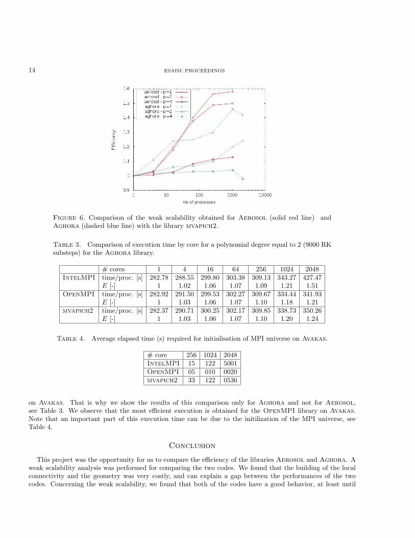
3.3. Results

Table 2 presents a weak scalability analysis where we evaluate the elapsed time observed for the globalcomputation and for a fixed number of 24 × 24 hexahedral elements per computing core. Results are shownas a function of the number of cores. The relative increase, E, of the elapsed time with respect to the singlecore is also indicated on Figure 6. Note that the memory requirement increases with the polynomial degree:the number of degrees of freedom per core is 4608, 15552, 36864, 72000 for p = 1, 2, 3 and 4, respectively. Weobserve that the solver scales nearly perfectly for p = 4, while results deteriorate for lower polynomial degreesp = 1 and 2. Aerosol has a stronger work load for boundary sides, because in Aghora, the boundary sidesof the top and the bottom are ignored in the boundary side loop, whereas in Aerosol, a freestream boundarycondition was used.

3.3.1. Analysis of the single core results

If we focus on the single core results, we see that Aerosol is between two and three times more costly thatAghora. Actually the results found during the CEMRACS project were even worse, for two reasons:

(1) The library Aerosol is based on the high level library PaMPA. This library gives iterators that allowsto loop on elements, faces, neighboring elements of faces, etc... In a first version of the code, PaMPA

iterators were used for all the loops. The results on a single core, without optimization options, gave anexecution time of 977.3 s for p = 1, and of 5938.6 s for p = 2. A new version was developed, where theconnectivity is stored, and where PaMPA iterators are used only once for building the connectivity.Execution time was improved from 977.3 to 391.93 s for p = 1, and from 5938.6 s to 1450.59 s for p = 2.

(2) The first tests we did were done without activating compiler optimization options. These optimizationsand some other classical tricks (removing some checkings, avoiding the call to complex C++ datastructures, and using local registers) decreased the execution time from 391.93 s to 49.2 s for p = 1 andfrom 1450.59 s to 170.14 s for p = 2.


Table 1. Yee vortex problem: relative costs in percent of different stages of the numericalalgorithm per physical time step on one process.

p 1 2 4Aerosol Aghora Aerosol Aghora Aerosol Aghora

boundary surface integral 28.9 4.2 20.3 3.2 9.5 2.2internal surface integral 47.4 57.5 31.2 46.8 15.8 34.6volume integral 23.1 36.5 48.1 49.3 74.5 63.0mass matrix inversion 0.6 1.8 0.4 0.7 0.2 0.2

Table 2. Yee vortex problem: time/proc. [s] with Aerosol and Aghora for 3000 Runge-Kuttasubsteps with the MPI distribution mvapich2.

# cores 1 4 16 64 256 1024 2048p = 1 Aghora 12.67 14.02 15.69 15.88 16.42 18.43 17.97

Aerosol 49.20 50.76 57.97 69 76.97 77.8p = 2 Aghora 94.12 96.90 100.08 100.72 103.28 112.91 116.75

Aerosol 170.14 175.1 204.19 234.41 253.37 255.07p = 4 Aghora 1401.5 1421.3 1430.2 1435.5 1439.1 1451.4 1370.8

Aerosol 2079.3 2093.7 2134.8 2252.2 2315.3 2349.4

As far as the remaining difference on a single core between Aerosol and Aghora is concerned (see first columnof Table 2), we attribute this to the strategy of stocking all the geometry instead of recomputing it at each timestep, as explained in Section 2.3.1.

3.3.2. Analysis of the scalability

Table 1 gives a detailed analysis of the relative costs of different stages of the numerical algorithm. Resultsare given for one core. The implementation of surface and volume integrals for fluxes clearly represents themost expensive stage and its relative cost increases with p. This result is in agreement with the high scalabilityobserved for high p-values as local operations strongly dominate communications.

Weak scalability results are shown on Figure 6. The worse efficiency is obtained for Aerosol with p = 1, andthe most efficient is Aghora with p = 4. As explained in Section 2.3.3, communications are not implementedthe same way in Aerosol and in Aghora. In Aghora, point-to-point non blocking communications are used,whereas collective communications sent on Pthread are used in Aerosol. It was not obvious to predict whichcommunications would be the fastest:

• on one side, point-to-point communications send and receive the least data that are shared between twoprocesses

• on the other side, collective communications send all the overlaps to all the processes. This meansthat processes receive some parts of the overlap they do not need. These collective communications arenon-blocking because they are sent by a Pthread. Moreover, they might be more efficiently broadcastthan with (MPI Issend / MPI Irecv) if the MPI distribution uses a tree broadcast algorithm.

Our conclusion for the test we did is that point-to-point communications are more efficient than collectivecommunication sent on a Pthread.

3.3.3. Influence of the MPI distribution used on the performances

Last, we want to compare the results obtained with different MPI libraries; however, Aerosol needs anMPI library for which the MPI THREAD MULTIPLE is supported (i.e. if the process is multithreaded, multiplethreads may call MPI at once with no restrictions), and such a functionality is only available with mvapich2


Figure 6. Comparison of the weak scalability obtained for Aerosol (solid red line) andAghora (dashed blue line) with the library mvapich2.

Table 3. Comparison of execution time by core for a polynomial degree equal to 2 (9000 RKsubsteps) for the Aghora library.

# cores 1 4 16 64 256 1024 2048IntelMPI time/proc. [s] 282.78 288.55 299.80 303.38 309.13 343.27 427.47

E [-] 1 1.02 1.06 1.07 1.09 1.21 1.51OpenMPI time/proc. [s] 282.92 291.50 299.53 302.27 309.67 334.44 341.93

E [-] 1 1.03 1.06 1.07 1.10 1.18 1.21mvapich2 time/proc. [s] 282.37 290.71 300.25 302.17 309.85 338.73 350.26

E [-] 1 1.03 1.06 1.07 1.10 1.20 1.24

Table 4. Average elapsed time (s) required for initialisation of MPI universe on Avakas.

# core 256 1024 2048IntelMPI 15 122 5001OpenMPI 05 010 0020mvapich2 33 122 0536

on Avakas. That is why we show the results of this comparison only for Aghora and not for Aerosol,see Table 3. We observe that the most efficient execution is obtained for the OpenMPI library on Avakas.Note that an important part of this execution time can be due to the initilization of the MPI universe, seeTable 4.

Conclusion

This project was the opportunity for us to compare the efficiency of the libraries Aerosol and Aghora. Aweak scalability analysis was performed for comparing the two codes. We found that the building of the localconnectivity and the geometry was very costly, and can explain a gap between the performances of the twocodes. Concerning the weak scalability, we found that both of the codes have a good behavior, at least until


1024 cores. We compared two ways of doing non blocking communications: point-to-point communications,and collective communications sent on a Pthread. In our test, point-to-point communications were found tobe more efficient.

Further than the results presented here, this project allowed us to have discussions on the way to developand to factorize the code, that are difficult to account for here.

Acknowledgements Part of the computer time for this study was provided by the computing facilitiesMCIA (Mesocentre de Calcul Intensif Aquitain, on the cluster Avakas) of the Universite de Bordeauxand of the Universite de Pau et des Pays de l’Adour. Part of the computations have been performed at theMesocentre d’Aix-Marseille Universite.

References

[1] R. Abgrall. A review of residual distribution schemes for hyperbolic and parabolic problems : the July 2010 state of the art.

Commun.Comput.Phys., 11(4):1043–1080, 2012.[2] R. Abgrall, G. Baurin, P. Jacq, and M. Ricchiuto. Some examples of high order simulations of inviscid flows on unstructured

hybrid meshes by residual distribution schemes. Computers & Fluids, 61:1–13, 2012.[3] R. Abgrall, A. Larat, and M. Ricchiuto. Contruction of very high order residual distribution for steady inviscid flow problems

on hybrid unstructured meshes. J.Comput.Phys., 230(11):4103–4136, 2011.[4] R. Abgrall and P.L. Roe. High-order fluctuation schemes on triangular meshes. J. Sci. Comput., 19(3):3–36, 2003.

[5] F. Bassi, L. Botti, A. Colombo, D. A. Di Pietro, and P. Tesini. On the flexibility of agglomeration based physical spacediscontinuous Galerkin discretizations. J. Comput. Phys., 231(1):45–65, 2012.

[6] F Bassi, A Crivellini, S Rebay, and M Savini. Discontinuous Galerkin solution of the Reynolds-averaged Navier-Stokes andk−ω turbulence model equations. Computers & Fluids, 34(4-5):507–540, MAY-JUN 2005. Workshop on Residual DistributionSchemes, Discontinuous Galerkin Schemes, Multidimensional Schemes and Mesh Adaptation, Univ Bordeaux I, Inst Math,Talence, FRANCE, JUN 23-25, 2002.

[7] F. Bassi and S. Rebay. A high-order accurate discontinuous finite element method for the numerical solution of the compressibleNavier-Stokes equations. J. Comput. Phys., 131(2):267–279, 1997.

[8] R. Biswas, K. D. Devine, and J. Flaherty. Parallel, adaptive finite element methods for conservation laws. Appl. Numer. Math.,

14:255–283, 1994.[9] Alexander N. Brooks and Thomas J. R. Hughes. Streamline upwind/Petrov-Galerkin formulations for convection dominated

flows with particular emphasis on the incompressible Navier-Stokes equations. Comput. Methods Appl. Mech. Engrg., 32(1-3):199–259, 1982. FENOMECH ’81, Part I (Stuttgart, 1981).

[10] Guy Chavent and Bernardo Cockburn. The local projection P 0P 1-discontinuous-Galerkin finite element method for scalarconservation laws. RAIRO Model. Math. Anal. Numer., 23(4):565–592, 1989.

[11] Bernardo Cockburn and Chi-Wang Shu. Runge-Kutta discontinuous Galerkin methods for convection-dominated problems. J.Sci. Comput., 16(3):173–261, 2001.

[12] Ronald Cools. An encyclopaedia of cubature formulas. J. Complexity, 19(3):445–453, 2003. Numerical integration and its

complexity (Oberwolfach, 2001).[13] H. Deconinck and M. Ricchiuto. Residual distribution schemes: foundation and analysis. In E. Stein, R. de Borst, and T.J.R.

Hughes, editors, Encyclopedia of Computational Mechanics. John Wiley & Sons, Ltd., 2007. DOI: 10.1002/0470091355.ecm054.[14] Moshe Dubiner. Spectral methods on triangles and other domains. J. Sci. Comput., 6(4):345–390, 1991.

[15] Ami Harten, Stanley Osher, Bjorn Engquist, and Sukumar R. Chakravarthy. Some results on uniformly high-order accurateessentially nonoscillatory schemes. Appl. Numer. Math., 2(3-5):347–377, 1986.

[16] Guang Shan Jiang and Chi-Wang Shu. On a cell entropy inequality for discontinuous Galerkin methods. Math. Comp.,62(206):531–538, 1994.

[17] Norbert Kroll, Heribert Bieler, Herman Deconinck, Vincent Couaillier, Harmen van der Ven, and Kaare Sørensen, editors.ADIGMA - A European Initiative on the Development of Adaptive Higher-Order Variational Methods for Aerospace Appli-

cations, volume 113 of Notes on Numerical Fluid Mechanics and Multidisciplinary Design Volume. Springer, 2010.

[18] Jean-Francois Remacle, Joseph E. Flaherty, and Mark S. Shephard. An adaptive discontinuous Galerkin technique with anorthogonal basis applied to compressible flow problems. SIAM Rev., 45(1):53–72 (electronic), 2003.

[19] P.L. Roe. Fluctuations and signals - a framework for numerical evolution problems. In K.W. Morton and M.J. Baines, editors,Numerical Methods for Fluids Dynamics, pages 219–257. Academic Press, 1982.

[20] Chi-Wang Shu and Stanley Osher. Efficient implementation of essentially nonoscillatory shock-capturing schemes. J. Comput.

Phys., 77(2):439–471, 1988.

[21] Pavel Solın, Karel Segeth, and Ivo Dolezel. Higher-order finite element methods. Studies in Advanced Mathematics. Chapman& Hall/CRC, Boca Raton, FL, 2004. With 1 CD-ROM (Windows, Macintosh, UNIX and LINUX).


[22] Raymond J. Spiteri and Steven J. Ruuth. A new class of optimal high-order strong-stability-preserving time discretizationmethods. SIAM J. Numer. Anal., 40(2):469–491 (electronic), 2002.

[23] A. H. Stroud. Approximate calculation of multiple integrals. Prentice-Hall Inc., Englewood Cliffs, N.J., 1971. Prentice-HallSeries in Automatic Computation.

[24] H. C. Yee, N. D. Sandham, and M. J. Djomehri. Low-dissipative high-order shock-capturing methods using characteristic-basedfilters. J. Comput. Phys., 150(1):199–238, 1999.

[25] Linbo Zhang, Tao Cui, and Hui Liu. A set of symmetric quadrature rules on triangles and tetrahedra. Journal of Computational

Mathematics, 27(1):89–96, JAN 2009.

comparison of high order algorithms in aerosol and … · comparison of high order algorithms in...

Documents