comparison of h8 and -synthesis control design for quarter
TRANSCRIPT
International Journal of Scientific Research and Engineering Development-– Volume 3 Issues 1 Jan- Feb 2020
Available at www.ijsred.com
ISSN : 2581-7175 ©IJSRED: All Rights are Reserved Page 596
Comparison of H∞ and µ-synthesis Control Design for Quarter
Car Active Suspension System using Simulink
Mustefa Jibril*, Tesfabirhan Shoga**
*(Department of Electrical & Computer Engineering, DireDawa Institute of Technology, DireDawa, Ethiopia
Email: [email protected])
** (Department of Electrical & Computer Engineering, Jimma Institute of Technology, Jimma, Ethiopia
Email: [email protected])
----------------------------------------************************----------------------------------
Abstract: To improve road dealing with and passenger consolation of a vehicle, a suspension system is supplied. An
active suspension system is taken into consideration better than the passive suspension system. In this
paper, an active suspension system of a linear quarter vehicle is designed, that's issue to exclusive
disturbances on the road. Since the parametric uncertainty within the spring, the shock absorber and the
actuator has been taken into consideration, robust control is used. H∞ and µ-Synthesis controllers of are
used to improve using consolation and road dealing with potential of the vehicle, in addition to confirm the
sturdy stability and overall performance of the system. In the H∞ design, we designed a driving force for
passenger consolation and to preserve the deflection of the suspension small and to reduce the disturbance
of the road to the deflection of the suspension. For the µ synthesis system, we designed a controller with
hydraulic actuator and uncertainty model. We designed a MATLAB / SIMULINK model for the active
suspension system with the H∞ and µ-synthesis controllers we tested the use of 4 road disturbance inputs
(bump, random, sinusoidal pavement and slope) for deflection of the suspension, body acceleration and
body travel for passive, active suspension with controller and active suspension without controller. Finally,
we evaluate the H∞ and µ-synthesis controllers with a Simulink model for suspension deflection, body
acceleration and body travel simulation, and the result suggests that both designs offer correct overall
performance, however the H∞controller has superior overall performance as compared to the µ-synthesis
controller.
Keywords —Quarter Car Active Suspension System, H∞ Controller, µ−Synthesis Controller, Robust
Performance, Robust Stability
----------------------------------------************************----------------------------------
I. INTRODUCTION
At present, the arena's leading automotive agencies
and studies establishments have invested huge
human and material assets to increase a value-
effective vehicle suspension system, to be widely
used within the vehicle. The principal cause of the
suspension system is to isolate the vehicle body
from the irregularities of the road to maximize
passenger consolation and preserve continuous road
wheel touch to provide avenue grip. Many studies
have proven that vibrations because of abnormal
avenue surfaces have an effect of draining energy in
drivers, affecting their physical and intellectual
health [1]. The needs for extra driving consolation
and manage capacity of road, consisting of vehicles,
have encouraged the improvement of recent styles
of suspension systems, consisting of active and
semi-active suspension systems. These
electronically managed suspension structures can
RESEARCH ARTICLE OPEN ACCESS
International Journal of Scientific Research and Engineering Development-– Volume 3 Issues 1 Jan- Feb 2020
Available at www.ijsred.com
ISSN : 2581-7175 ©IJSRED: All Rights are Reserved Page 597
probably enhance riding comfort, in addition to
riding the vehicle on the road. An active suspension
system has the capability to constantly adjust to
converting road situations. By converting its
character to reply to variable road situations, the
active suspension offers advanced dealing with,
road experience, responsiveness and protection.
An active suspension system has the potential to
constantly regulate to changing road conditions. By
converting its body or wheel to reply to
extraordinary road situations, the active suspension
gives advanced managing, road feel, responsiveness
and safety.
Active suspension structures respond dynamically
to changes in the road profile because of their
capability to supply strength that may be used to
produce relative movement among the body and the
wheel.
Typically, active suspension systems include
sensors to measure suspension variables, such as
body velocity, suspension displacement and wheel
pace, and wheel and body acceleration.
An active suspension is one wherein the passive
components are augmented through actuators that
offer extra forces. These extra forces are decided by
means of a feedback manage regulation that uses
sensor statistics connected to the vehicle.
The current active suspension system is inefficient
if there are changes inside the system or actuator
parameters, then controlling the suspension system
will become a massive hassle. Therefore, H∞ and
µ-synthesis control strategies of are used. The H∞
and µ-synthesis manipulate of successfully
suppresses car vibrations inside the touchy
frequency variety of the human body. The desired
robust overall performance and strong stability are
carried out inside the closed loop system for an
quarter vehiclesystem within the presence of
structured uncertainties.
II. MATHEMATICAL MODELS A. Passive Suspension System Mathematical Model
The design of the vibration control system have to
start with the status quo of the mathematical model
of the system after which decide the design
necessities and the formal description of the system.
And then choose one or extra layout techniques to
design the control system, and then connect it to the
simulation or model experiments to become aware
of that the manipulate system is designed to satisfy
the performance requirements. Therefore, the
establishment of the mathematical models of the
system is a prerequisite for all manipulate designs
and the layout of the manipulate system is intently
related to the satisfactory assessment model of the
system.
As with other engineering control systems, a
mathematical version of the suspension
controlsystem refers back to the formal version, to
abbreviate the mathematical model. These models
are typically based at the dynamic precept so as to
be derived or through a number of the dynamics
assessments of the system. Then it
experiencesmathematical simulation and
optimization, or statistical approach. The key to
develop a mathematical model system is to offer a
description of the model form and decide its
parameters.
In the area of vibration control, there are three
maximum popular sorts of fashions to explain the
form, the description of the popularity area, the
description of the transfer function and the
description of the weight function. According to the
implementation of time continuous manipulate and
discrete timecontrol of various traits, each of them
is divided into a time continuous and discrete
mathematical description over.
The automobile is a complex vibration system, it
should be simplified depending on the hassle
evaluation. There are numerous approaches to
simplify motor vehicles, but in line with the
convenience of the have a look at, we simplify in
this paper to a system model as shown in Figure 1
below:

International Journal of Scientific Research and Engineering Development-– Volume 3 Issues 1 Jan- Feb 2020
Available at www.ijsred.com
ISSN : 2581-7175 ©IJSRED: All Rights are Reserved Page 598
Fig. 1. Quarter Model of Passive suspension system
Figure 1 shows a quarter vehicle model of the
passive suspension system. The suspended mass m1
represents the body of the car, and the non-
suspended mass m2 is an axle and wheel meeting. It
guarantees that the tire comes into touch with the
road floor while the vehicle is in movement, and is
modeled as a linear spring with stiffness. The linear
damper, whose common damping coefficient is D,
and the linear spring, whose common stiffness
coefficient is k1, include the passive factor of the
suspension system. The state variables x0 (t) and xb
(t) are the vertical displacements of the sprung and
unsprung masses, respectively, and xi (t) is the
vertical road profile.
This is a version of dual mass vibration system of
the body and the wheel of the car. From this
version, we will examine the dynamics of the
automobile suspension system and establishdegree
of freedom of differential equations of motion. Its
equilibrium role is the beginning of the coordinates;
we can get the equations as follows (1) and (2).
( ) ( ) ( ) ( ) ( ) ( )
..
. .
1 0 0 1 0 0 1b b
m x t D x t x t k x t x t
+ − + − = &&
( ) ( ) ( ) ( ) ( ) ( ) ( ) ( ).. . .
2 0 1 0 2 0 2b b b b im x t D x t x t k x t x t k x t x t
− − + − + − =
Letting
W = x 0− xb
W Suspension Deflection
Xi Road Disturbance
If we make a Laplace transformation to the above
equation, we can get equation (3):
( ) ( )( )1 2
2
1 2 2 2 2 1 1 1 2 2 1 2
3i
M KW
X M M s M K Ds M K M K M K K K=
+ + + + + +
Table I: Parameters of quarter vehicle model
Model parameters symbol symbol Values
Vehicle body mass m 1 300 Kg
Wheel assembly mass m 2 40 Kg
Suspension stiffness k 1 15,000 N/m
Tire stiffness k 2 150,000 N/m
Suspension damping D 1000 N-s/m
The passive suspension system PC1 (s) transfer
function is
( )9
1 2 8 9
4.5 10
12000 1.5 10 2.261 10CP s
s s
×=
+ × + ×
B. Active Suspension System Mathematical Model
The mathematical model and the simulation
accomplished within the following sections
handiest discuss the amount of force created by
using the active suspension. Active suspensions
permit the designer to balance these goals the usage
of a hydraulic actuator with comments controller
that is pushed by using a motor among the chassis
and the wheel assembly. The force U implemented
between the body and the wheel meeting is
controlled by comments and represents the active
element of the suspension system.
Fig. 2. Quarter Model of active suspension system with actuating force (u)
between sprung and unsprung mass.
Figure 2 shows a quarter vehicle model of the
active suspension system. The mass m 1 (in
kilograms) represents the vehicle chassis (body)
and the mass m 2 (in kilograms) represents the
wheel assembly. The spring K 1 and the shock
absorber D represent the passive spring and the
surprise absorber placed among the vehicle body
and the wheel assembly. The K2 spring fashions the
compressibility of the tire. The

International Journal of Scientific Research and Engineering Development-– Volume 3 Issues 1 Jan- Feb 2020
Available at www.ijsred.com
ISSN : 2581-7175 ©IJSRED: All Rights are Reserved Page 599
variables x 0 , x b and x i (all in meters) are the
body travel, wheel travel, and road disturbance,
respectively. The actuator pressure f s (in Kilo
Newton’s) implemented between the body and the
wheel assembly is controlled through feedback and
represents the active component of the suspension
system.
From this model, we will examine the dynamics of
the vehicle suspension system as a linear
systemmodel and set up2 degree of freedom. The
differential equations of movement could be as
follows:
( ) ( ) ( ) ( ) ( )1 0 0 2 1 0 2m x t D x t x t k x t x t u+ − + − = && & &
( ) ( ) ( )[ ] ( ) ( )[ ] ( ) ( )[ ]2 2 0 2 1 2 0 2 2 1m x t D x t x t k x t x t k x t x t u− − + − + − = −&& & &
We can set:
( ) ( ) ( ) ( )1 2 2 0 3 2 4 0, , ,x x t x x t x x t x x t= = = =& &
The system state space equation can be express as:
dXAX BU
dt= +
In this equation, state variable matrixes are:
( )1 2 3 4
TX x x x x=
Constant matrixes A and B are shown as below:
1 2 1
2 2 2 2
1 1
1 1 1 1
0 0 1 0
0 0 0 1
k k k D DA
m m m m
k k D D
m m m m
+
− −=
− −
2
2 2
1
0 0
0 0
1
10
kB
m m
m
=
−
The system input variable matrix will be:
( )( )1
T
U x t u=
The vehicle suspension system output matrix
equation will be:
Y CX DU= +
In above equation, the output variable matrix Y will
be:
( ) ( ) ( ) ( )( )2 1 2 0 0Y k x t x t x t x t= − &&
Y will also express as the following equation:
( ) ( ) ( ) ( )( )2 1 2 0 0Y k x t x t x t x t= − &&
Constant matrixes C and D will be shown as below:
2
1 1
1 1 1 1
0 0 0
0 1 0 0
k
k k D DC
m m m m
− = − −
2
1
0
10
0 0
k
Dm
= −
III. ROAD PROFILES
Four types of road disturbance input are used to
simulate distinctive forms of road conditions. They
are bump input signal, sine pavement input signal,
random input signal and slope road input signal.
These entries are the prerequisite for simulating the
vehicles suspension system, and should correctly
mirror the real circumstance of the road while a
vehicle is touring on the street. The specific signal
is important to the simulation result. We expect that
the car is a linear system.
A. Bump Road Disturbance:
The bump input signal is a primary input to
investigate the suspension system. It simulated a
completely extreme pressure for a totally short
time, along with riding a car thru a speed hump.
This road disturbance has a maximum peak of 10
cm as shown in Figure 3.

International Journal of Scientific Research and Engineering Development
©IJSRED: All Rights are Reserved
Fig. 3. Bump road disturbance
B. Random Road Disturbance:
Numerous investigations display that it's miles
important to check a car with a random disturbance
of the road to verify that the spring and the surprise
reply quickly and effectively. The random
disturbance of the road has a maximum peak of 10
cm and a minimum peak of zero cm as shown in
Figure 4.
Fig. 4. Random road disturbance
C. Sine Pavement Road Disturbance:
The sine wave input signal can be used to simulate
periodic pavement fluctuations. You can test the
resilience of the vehicle's suspension system while
the auto reviews periodic wave pavement. The
sinusoidal access pavement test is executed by
using all automotive industries before a brand new
vehicle drives on the street. The alteration of the
sinusoidal pavement road has a height of
10 cm, as shown in Figure 5.
International Journal of Scientific Research and Engineering Development-– Volume 3 Issues 1 Jan
Available at www.ijsred.com
©IJSRED: All Rights are Reserved
Numerous investigations display that it's miles
important to check a car with a random disturbance
that the spring and the surprise
reply quickly and effectively. The random
disturbance of the road has a maximum peak of 10
cm and a minimum peak of zero cm as shown in
ave input signal can be used to simulate
periodic pavement fluctuations. You can test the
resilience of the vehicle's suspension system while
the auto reviews periodic wave pavement. The
sinusoidal access pavement test is executed by
ndustries before a brand new
vehicle drives on the street. The alteration of the
sinusoidal pavement road has a height of -10 cm to
Fig. 5. Sine Input pavement road disturbance
D. Slope Road Disturbance:
The performance of the suspension is tested using
the disturbance of the slope of the road through
verifying the degree of elevation of the road that
drives the suspension. The slope road disturbance at
the has an elevation of 45 degree as shown in
Figure 6.
Fig. 6. Slope road disturbance
IV. THE PROPOSED H
DESIGN
A. H infinity Controller Design Gc1 (s):
The design of the active suspension system to offer
consolation to passengers and driving on the road is
advanced the usage of the design of the H
controller. The essential objective of the controller
design is to reduce suspension deflection, body
acceleration and body travel. H
approach used to design the proposed controller
attaining the performance goal by means of
minimizing the norm of the weighted transfer
Volume 3 Issues 1 Jan- Feb 2020
www.ijsred.com
Page 600
Fig. 5. Sine Input pavement road disturbance
suspension is tested using
the disturbance of the slope of the road through
verifying the degree of elevation of the road that
drives the suspension. The slope road disturbance at
the has an elevation of 45 degree as shown in
disturbance
THE PROPOSED H ∞ CONTROL
(s):
The design of the active suspension system to offer
consolation to passengers and driving on the road is
advanced the usage of the design of the H ∞
controller. The essential objective of the controller
design is to reduce suspension deflection, body
eration and body travel. H ∞ synthesis is the
approach used to design the proposed controller
attaining the performance goal by means of
minimizing the norm of the weighted transfer

International Journal of Scientific Research and Engineering Development-– Volume 3 Issues 1 Jan- Feb 2020
Available at www.ijsred.com
ISSN : 2581-7175 ©IJSRED: All Rights are Reserved Page 601
function. The interconnected H ∞ design for the
active suspension system is shown in Figure 7.
Fig. 7. H ∞ system interconnected block diagram
There are two purposes for the weighted function
widespread: for a given general, there could be an
immediate contrast for extraordinary overall
performance targets and they may be used to
recognize the frequency records incorporated in the
analysis. The output or feedback signaly is
y = (x 4 + d2∗Wn) ∗H∞ Controller
The controller acts on the y signal and to produce
the road disturbance signal. The Wn block modeled
the sensor noise within the channel. Wn given a
sensor noise of 0.05 m.
Wn = 0.05
Wn is used to model the noise of the displacement
sensor. The magnitude of the active control force is
scaled using the Wref. Let us assume the maximum
control force is 0.1Newton which means
Wref = 0.1
The weighting function Wact is used to limit the
magnitude and frequency content of the input road
disturbance signal. Choosing
80 60
11 600act
sW
s
+=
+
Wx1 and Wx1−x3 are used to keep the car deflection
and the suspension deflection small over the desired
range. The car body deflection Wx1 is given as
1
508.1
56.55x
Ws
=+
The suspension deflection is used via weighting
functionWx1−x3. The weighting function is given as
1 3
15
0.2 1x xW
s−
=+
B. The Proposed µ-Synthesis Control Design
In the active suspension system, the µ-synthesis
design included the dynamics of the hydraulic
actuator. To recall the difference between the
actuator model and the actual actuator dynamics,
we use a first-order model of the actuator dynamics,
as well as an uncertainty model. The block diagram
of µ-synthesis controller system interconnection for
the active suspension system is shown in Figure 8.
Fig. 8. µ-synthesis interconnection block diagram
C. µ-Synthesis Controller Design Sc1 (s):
The nominal model for the hydraulic actuator is
1
11
50
actHYD
s
=
+
We describe the error of the actuator model as a
hard and fast of feasible fashions that use a
weighting functions because the actuator model
itself is uncertain. The uncertainty of the model is
represented with the aid of the Wunc weight that
corresponds to the frequency variation of the
uncertainty of the model and the object of uncertain
LTI dynamics object 4unc which is Unc=Uncertain
LTI dynamics ”unc” with 1 outputs, 1 inputs, and
gain less than 1.

International Journal of Scientific Research and Engineering Development
©IJSRED: All Rights are Reserved
0.03 0.15
0.001667 1unc
sW
s
+=
+
The uncertain actuator model represents the
hydraulic actuator model used for the control. A µ
synthesis controller is synthesized using
iteration. The D-K iteration approach is a method to
synthesis that attempts to synthesize the controller.
There are two control inputs: the road disturbance
signal and and the active control force
three measurement output signals, the
deflection, car body acceleration and car body
travel.
V. Result and Discussion A. Simulation of the Proposed Controllers
In this subsection we simulate passive suspension
system, active suspension system with
controller, active suspension system with
controller and active suspension system without
controller for suspension deflection, body
acceleration and body travel using bump, random,
sine pavement and slope road disturbances.
B. Simulation of a Bump Road Disturbance:
The Simulink model for a bump input road
disturbance and active control force input is shown
in Figure 9. In this Simulink model, we simulate
passive suspension system, active suspension
system with G C1 (s) controller, active suspension
system with SC1 (s) controller and active suspension
system without controller for suspension deflection,
body acceleration and body travel. Here in this
Simulink we assign d1 and d2 as a random signal
with amplitude of 0.001 and period of 10 seconds
and there are three error signals named e1, e2 and
e3 and there are three active control force for the
active suspension with controller and without
controller with a step function input.
International Journal of Scientific Research and Engineering Development-– Volume 3 Issues 1 Jan
Available at www.ijsred.com
©IJSRED: All Rights are Reserved
represents the
hydraulic actuator model used for the control. A µ-
using the D-K
approach is a method to
size the controller.
control inputs: the road disturbance
and the active control force. There are
three measurement output signals, the suspension
deflection, car body acceleration and car body
In this subsection we simulate passive suspension
system, active suspension system with GC1 (s)
controller, active suspension system with SC1 (s)
controller and active suspension system without
controller for suspension deflection, body
acceleration and body travel using bump, random,
sine pavement and slope road disturbances.
Road Disturbance:
The Simulink model for a bump input road
disturbance and active control force input is shown
in Figure 9. In this Simulink model, we simulate
passive suspension system, active suspension
) controller, active suspension
) controller and active suspension
system without controller for suspension deflection,
body acceleration and body travel. Here in this
Simulink we assign d1 and d2 as a random signal
with amplitude of 0.001 and period of 10 seconds
there are three error signals named e1, e2 and
e3 and there are three active control force for the
active suspension with controller and without
Fig. 9. Simulink model of a Bump road disturbance
The suspension deflection, body acceleration and
body travel simulation output is shown in Figure
10, Figure 11 and Figure 12 respectively for a bump
road disturbance and active control force inputs.
Fig. 10. Suspension deflection for Bump road disturbance
Fig. 11. Body acceleration for Bump road disturbance
Volume 3 Issues 1 Jan- Feb 2020
www.ijsred.com
Page 602
Fig. 9. Simulink model of a Bump road disturbance
deflection, body acceleration and
body travel simulation output is shown in Figure
10, Figure 11 and Figure 12 respectively for a bump
road disturbance and active control force inputs.
Fig. 10. Suspension deflection for Bump road disturbance
ody acceleration for Bump road disturbance
International Journal of Scientific Research and Engineering Development-– Volume 3 Issues 1 Jan- Feb 2020
Available at www.ijsred.com
ISSN : 2581-7175 ©IJSRED: All Rights are Reserved Page 603
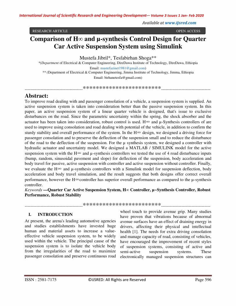
Fig. 12. Body travel for Bump road disturbance
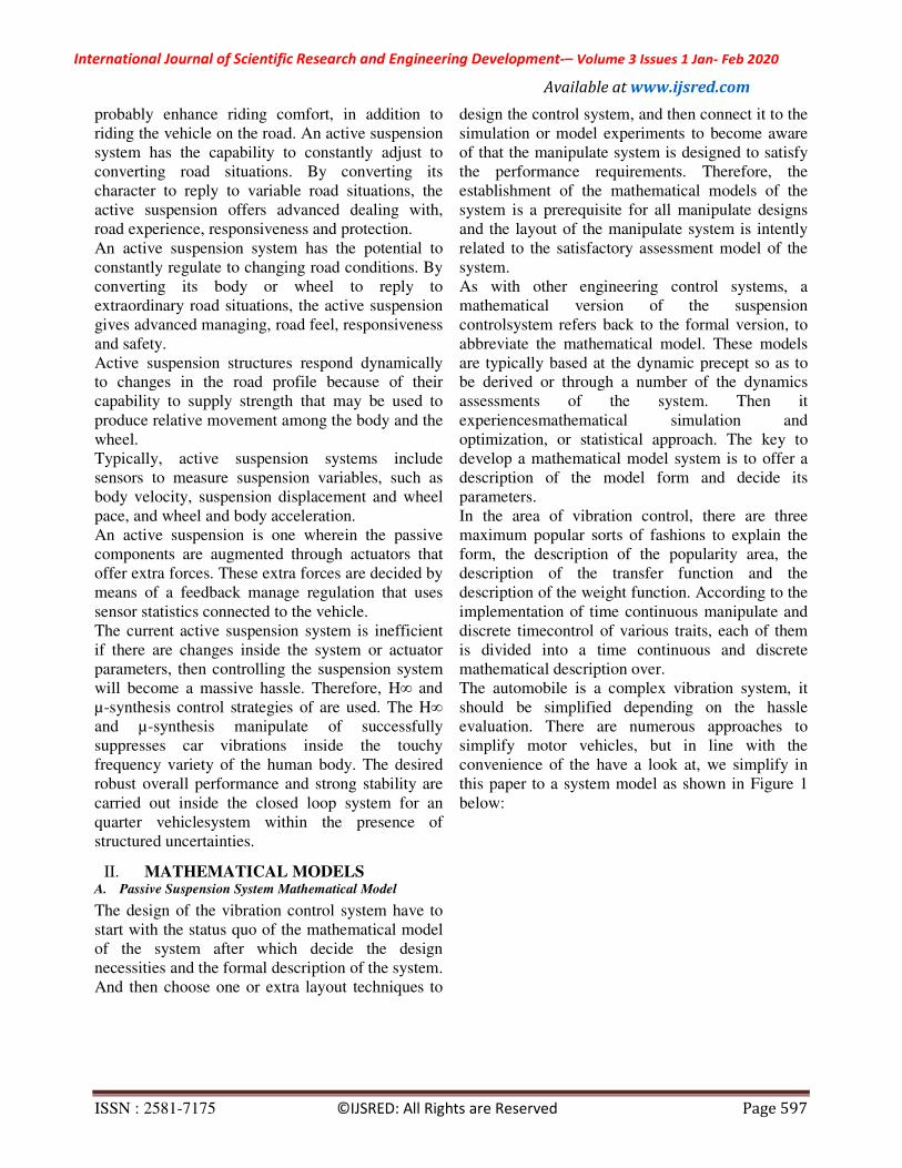
C. Simulation of a Random Road Disturbance:
The Simulink model for a random road disturbance
and active control force inputs is shown in Figure
13.The suspension deflection, body acceleration
and body travel simulation is shown in Figure 14,
Figure 15 and Figure 16 respectively.
Fig. 13. Simulink model for a Random road disturbance
Fig.14.Suspension deflection for Random road disturbance
Fig. 15. Body acceleration for Random road disturbance
Fig. 16. Body travel for Random road disturbance
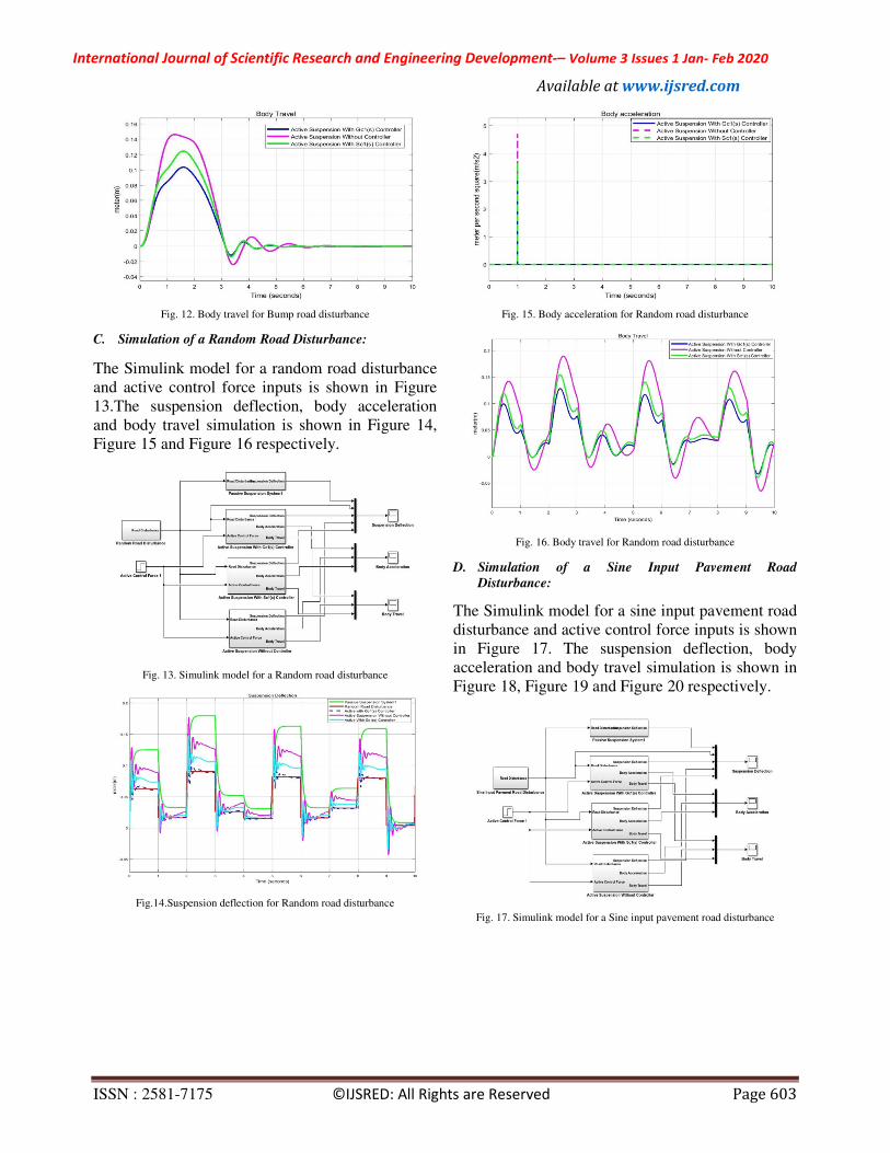
D. Simulation of a Sine Input Pavement Road
Disturbance:
The Simulink model for a sine input pavement road
disturbance and active control force inputs is shown
in Figure 17. The suspension deflection, body
acceleration and body travel simulation is shown in
Figure 18, Figure 19 and Figure 20 respectively.
Fig. 17. Simulink model for a Sine input pavement road disturbance

International Journal of Scientific Research and Engineering Development
©IJSRED: All Rights are Reserved
Fig. 18. Suspension deflection for Sine input pavement
Fig. 19. Body acceleration for Sine input pavement road disturbance
Fig. 20. Body travel for Sine input pavement road disturbance
E. Simulation of a Slope Road Disturbance:
The Simulink model for a slope road disturbance
and active control force inputs is shown in Figure
21.The suspension deflection, body acceleration
and body travel simulation is shown in Figure 22,
Figure 23 and Figure 24 respectively.
International Journal of Scientific Research and Engineering Development-– Volume 3 Issues 1 Jan
Available at www.ijsred.com
©IJSRED: All Rights are Reserved
Fig. 18. Suspension deflection for Sine input pavement road disturbance
Fig. 19. Body acceleration for Sine input pavement road disturbance
Fig. 20. Body travel for Sine input pavement road disturbance
Simulation of a Slope Road Disturbance:
The Simulink model for a slope road disturbance
ol force inputs is shown in Figure
21.The suspension deflection, body acceleration
and body travel simulation is shown in Figure 22,
Fig. 21. Simulink model for a Slope road disturbance
Fig. 22. Suspension deflection for Slope road disturbance
Fig. 23. Body acceleration for Slope road disturbance
Volume 3 Issues 1 Jan- Feb 2020
www.ijsred.com
Page 604
Fig. 21. Simulink model for a Slope road disturbance
on for Slope road disturbance
Fig. 23. Body acceleration for Slope road disturbance

International Journal of Scientific Research and Engineering Development-– Volume 3 Issues 1 Jan- Feb 2020
Available at www.ijsred.com
ISSN : 2581-7175 ©IJSRED: All Rights are Reserved Page 605
Fig. 24. Body travel for Slope road disturbance
F. Comparison of Active Suspension System With H∞ GC1
(s) and µ−Synthesis SC1 (s) Controllers
Here in this section, we compare active suspension
system with H∞ controller (GC1 (s)) and
µ−synthesis controller (SC1 (s)) for suspension
deflection, body acceleration and body travel with
bump, random, sine and slope road disturbances.
G. Comparison for Bump Road Disturbance:
In the suspension deflection simulation as shown in
Figure 10, the active suspension system with SC1 (s)
controller strokes are larger than the road surface
wave amplitude while the active suspension system
with GC1 (s) controller strokes fits the road surface
wave amplitude. In the body acceleration as shown
in Figure 11, the acceleration is effectively reduced
in the active suspension system with GC1 (s)
controller. In the body travel as shown in Figure 12,
the vertical distance that the body travels is
effectively reduced in the active suspension system
with GC1 (s) controller. The reduction in overshoot
value is shown in Table 2.
Table II Reduction in overshoot value for bump road disturbance
Parameters SC1 (s) GC1 (s) % in
Reduction
Suspension
Deflection
0.13 m 0.1 m 23.08 %
Body Acceleration
242
m
s 5
2
m
s
79.2 %
Body Travel 0.13m 0.11 m 15.38 %
H. Comparison for Random Road Disturbance:
In the suspension deflection simulation as shown in
Figure 14, the active suspension system with SC1 (s)
controller strokes have a larger amplitude than the
active suspension system with GC1 (s) controller. In
the body acceleration as shown in Figure 15, the
acceleration is effective reduced in the active
suspension system with GC1 (s) controller. In the
body travel as shown in Figure 16, the vertical
distance that the body travels is effectively reduced
in the active suspension system with GC1 (s)
controller. The reduction in overshoot value is
shown in Table III.
Table III Reduction in overshoot value for random road disturbance
Parameters SC1 (s) GC1 (s) % in
Reduction
Suspension
Deflection
0.18 m 0.13 m 27.78 %
Body Acceleration
3.72
m
s 3
2
m
s
19 %
Body Travel 0.16 m 0.13 m 18.75
I. Comparison for Sine Pavement Road Disturbance:
In the suspension deflection simulation as shown in
Figure 18, the active suspension system with SC1 (s)
controller strokes are larger than the road surface
wave amplitude while the active suspension system
with GC1 (s) controller strokes fits the road surface
wave amplitude. In the body acceleration as shown
in Figure 19, the acceleration is effectively reduced
in the active suspension system with GC1 (s)
controller. In the body travel as shown in Figure 20,
the vertical distance that the body travels has a large
amplitude in the active suspension system with SC1
(s) controller and is effectively reduced in the active
suspension system with GC1 (s) controller. The
reduction in overshoot value is shown in Table V.
Table V Reduction in overshoot value for sine pavement road disturbance
Parameters SC1 (s) GC1 (s) % in
Reduction
Suspension
Deflection
0.13 m 0.1 m 23.08 %
Body Acceleration
2.2
m
s 2.
2
m
s
4.56 %
Body Travel 0.14 m 0.12 m 14.3 %
J. Comparison for Slope Road Disturbance:
In the suspension deflection simulation as shown in
Figure 22, the active suspension system with SC1 (s)
controller slopes are larger than the road surface
wave amplitude while the active suspension system

International Journal of Scientific Research and Engineering Development-– Volume 3 Issues 1 Jan- Feb 2020
Available at www.ijsred.com
ISSN : 2581-7175 ©IJSRED: All Rights are Reserved Page 606
with GC1 (s) controller slope fits the road surface
wave amplitude. In the body acceleration as shown
in Figure 23, the acceleration is effectively reduced
in the active suspension system with GC1 (s)
controller. In the body travel as shown in Figure 24,
the body travels has a large slope and vibration in
the active suspension system with SC1 (s) controller
and is effectively aligned with small vibration in the
active suspension system with GC1 (s) controller.
The reduction in overshoot value is shown in Table
V.
Table V Reduction in overshoot value for slope road disturbance
Parameters SC1 (s) GC1 (s) % in Reduction
Suspension
Deflection
51.30 450 12.3 %
Body Acceleration
3.52
m
s 2
2
m
s
43 %
Body Travel 51.30 450 12.3 %
VI. CONCLUSION
In this paper, H ∞ controller and µ - synthesis
controllers are successfully designed using
MATLAB/SIMULINK for quarter car active
suspension system. We design a Simulink model
that represents the active suspension system with H
∞ controller, µ - synthesis controller, without
controller and passive suspension system and tasted
with bump, sine input pavement, random and slope
road disturbances for suspension deflection, body
acceleration and body travel. We compared the
active suspension system with H ∞ controller and µ
- synthesis controller for the three parameters and
we analyze the percentage reduction in overshoot of
the two controllers.
The simulation results shows that the active
suspension system with H ∞ controller is capable of
stabilizing the suspension system very effectively
than the active suspension system with µ - synthesis
controller for suspension deflection, body
acceleration and body travel parameters with the
four road input disturbances. The system with H ∞
controller has a percentage reduction in overshoot
than a system with µ - synthesis controller.
We conclude that an active suspension system with
H ∞ controller has the best performance with the
different tests we made on the system and it
achieves the passenger comfort and road handling
criteria that it needed to make the active suspension
system is the best suspension system.
ACKNOWLEDGMENTS
First and formost, I would like to express my
deepest thanks and gratitude to Dr.Parashante and
Mr.Tesfabirhan for their invaluable advices,
encouragement, continuous guidance and caring
support during my journal preparation.
Last but not least, I am always indebted to my
brother, Taha Jibril, my sister, Nejat Jibril and my
family members for their endless support and love
throughout these years. They gave me additional
motivation and determination during my journal
preparation.
REFERENCES [1]. Nasir, Ahmed and Al-awad “Genetic Algorithm Control of Model
Reduction Passive Quarter Car Suspension System” I.J. Modern
Education and Computer Science,Published Online February 2019. [2]. Vivek Kumar Maurya and Narinder Singh Bhangal “Optimal
Control of Vehicle Active Suspension System” Journal of
Automation and Control Engineering Vol. 6, No. 1, June 2018. [3]. MichielHaemers “Proportional-Integral State-Feedback Controller
Optimization for a Full-Car Active Suspension Setup using a
Genetic Algorithm” The 3rd IFAC Conference on Advances in
ProportionalIntegral-Derivative Control, Ghent, Belgium, May 9-
11, 2018.
[4]. Vinayak S. Dixit and Sachin C. Borse
“SemiactiveSsuspensionSsystem Design for QuarterCcar Model
and itsAanalysis with Passive Suspension Model” International
Journal of Engineering Sciences & Research Technology,February, 2017.
[5]. Yakubu G.1, Adisa A. B., “Simulation and Analysis of Active
Damping System for Vibration Control”, American Journal of Engineering Research, Vo. 6, Issue 11, 2017.
[6]. Ahmed A. Abougarair and Muawia M. A. Mahmoud “Design and
Simulation Optimal Controller for Quarter Car Active Suspension System” 1st Conference of Industrial Technology (CIT2017), 2017.
[7]. J. Marzbanrad and N. Zahabi “H∞ Active Control of a Vehicle
Suspension System Exited by Harmonic and Random Roads”
Journal of Mechanics and Mechanical Engineering Vol. 21, No. 1
pp 171–180, 2017.
[8]. Shital M. Pawar and A.A. Panchwadkar “Estimation of State
Variables of Active Suspension System using Kalman Filter”
International Journal of Current Engineering and Technology E-
ISSN 2277 – 4106 , P-ISSN 2347 – 5161,Vol.7, No.2, April, 2017.

International Journal of Scientific Research and Engineering Development-– Volume 3 Issues 1 Jan- Feb 2020
Available at www.ijsred.com
ISSN : 2581-7175 ©IJSRED: All Rights are Reserved Page 607
[9]. Libin Li and Qiang Li “Vibration Analysis Based on Full Multi Body Model for a Commercial Vehicle Syspension
System”ISPRA’07 Proceeding of the 6th WSEAS International
March 2016. [10]. NarinderSingh”Robust Control of Vehicle Active Suspension
System”International Journal of Control and Automation Vol. 9,
No. 4 (2016), pp. 149-160, 2016. [11]. Panshuo Li, James Lam, Kie Chung Cheung “Experimental
Investigation of Active Disturbance Rejection Control for Vehicle
Suspension Design”International Journal of Theoretical and
Applied Mechanics Volume 1, 2016.
[12]. Ahmed S Ali, GamalA.Jaber, Nouby M Ghazaly, “H∞ Control of
Active Suspension System for a Quarter Car Model”, International
Journal of Vehicle Structures and Systems Vol.8, No.1, 2016.
[13]. M. P. Nagarkar and G. J. VikhePatil “Multi-Objective
Optimization of LQR Control Quarter Car Suspension System using Genetic Algorithm” FME Transactions, 44, 187-196, 2016.