World Applied Sciences Journal 24 (9): 1234-1249, 2013ISSN 1818-4952© IDOSI Publications, 2013DOI: 10.5829/idosi.wasj.2013.24.09.1332

Corresponding Author: N. Abd. Rahman, Department of Chemical Engineering and Process, Faculty of Engineeringand Built Environment, Universiti Kebangsaan Malaysia, 43600 Bangi, Selangor, Malaysia.

1234

Comparison of Drying Parameter Optimization of Lemon Grass

N. Abd. Rahman, S.M. Tasirin, A.H.A. Razak, M. Mokhtar and S. MuslimDepartment of Chemical Engineering and Process, Faculty of Engineering

and Built Environment, Universiti Kebangsaan Malaysia, 43600 Bangi, Selangor, Malaysia

Submitted: Jul 22, 2013; Accepted: Sep 2, 2013; Published: Sep 11, 2013Abstract: The purpose of this study is to determine the optimum condition of humidity contents, drying rateand energy in the experiment of drying of lemon grass in the fluidized bed dryer with presence of inert particles.The studied drying parameters were temperature, air velocity, mass of sand and drying time. The optimizationmethods used in the studies were Taguchi, Pareto, ANOVA, XLSTAT and Design- Expert. Design of experiment(DOE) used in this study was three levels and three factors (3L3F) where L orthogonal array was implemented.27

DOE of three levels and four factors (3L4F) was applied for the optimization to observe the effect of drying timewhich implemented L orthogonal array. The temperatures were varied at 40°C, 50°C, 60°C; the air velocities81

were ranged at 0.61 m/s, 0.73 m/s, 0.85 m/s; mass of sand as an inert particle used in the experiment were 0 g,50 g and 100g. Lastly, the drying time was conducted at 10 min, 20 min and 30 min. In optimization process,Taguchi and Pareto ANOVA are the most appropriate statistical method to optimize the data due to its simplicityand no ANOVA table involved. For DOE of 3L3F, the optimum value of humidity contents was 0.0658 g/g aqwhich occurred at temperature of 60°C, air velocity of 0.85 m/s and 100g of sand. The optimum value of dryingrate was 0.2497 g/g min which occurred at temperature of 50°C, air velocity of 0.85 m/s and 50 g of sand. Finallythe optimum value of energy occurred at temperature of 40°C, air velocity of 0.61 m/s and 100 g of sand.

Key words: Drying Taguchi Pareto ANOVA XLSTAT Design Expert Lemon grass Optimization

INTRODUCTION problems. One of the commercially used dryer is fluidized

Drying is a process of removing the moisture content and it is suitable to be used in many fields and sectors [4].from a component which is either in the form of solid, half Furthermore, the existence of inert material will increasesolid, solution or slurry [1, 2]. This process can be said as the fluidization behaviour of the drying products [5].one of the oldest technology which nowadays becomes Inert materials will act as heat carrier and it transfers thevery common and important in our life. Drying plays an heat from the air into the products. Besides that, byimportant role in the field of chemical, agriculture, drying the products in a fluidized bed dryer and inertbiotechnology, food, polymer, ceramic, pharmaceutical, material, the quality of the products will be betterpaper and wood processing industry [3]. The main compared to sun drying. The fluidized bed dryer is thepurposes of drying are to increase the lifespan of a suitable equipment for the drying process since thecomponent (food), reduce the weight of the component drying is gently and direct heating is avoided.(clay soil) for easier delivery and change the form of a Scientific name for lemon grass is cymbopogoncomponent (detergent) so that it can be used and kept ciatrus. Recently, many researched have been done oneasily. lemon grass to study about its potential usage in our daily

Traditional method of drying by using sun light is life. Lemon grass is not only being used in cookingnot the best drying process as this brings up the purpose, but it contains some important component suchproblems of sanity and quality of the products. as citronellal, linalool and citronellol which might beHence, many dryers have been invented to overcome the useful in preserving food [6], replacing petrochemical for

bed dryer. Fluidized bed dryer has high thermal efficiency

World Appl. Sci. J., 24 (9): 1234-1249, 2013

1235

synthesizing of other chemical substances [7], medicinelike leukemia [8] as well as insecticide [9]. Hence, thisstudy will carry out the drying of lemon grass influidized bed dryer with the presence of inert materials.This objective is achieved by doing the comparison studyat different optimization methods (Taguchi, Pareto,ANOVA, XLSTAT and Design- Expert) and the optimumdrying conditions.

MATERIALS AND METHODS

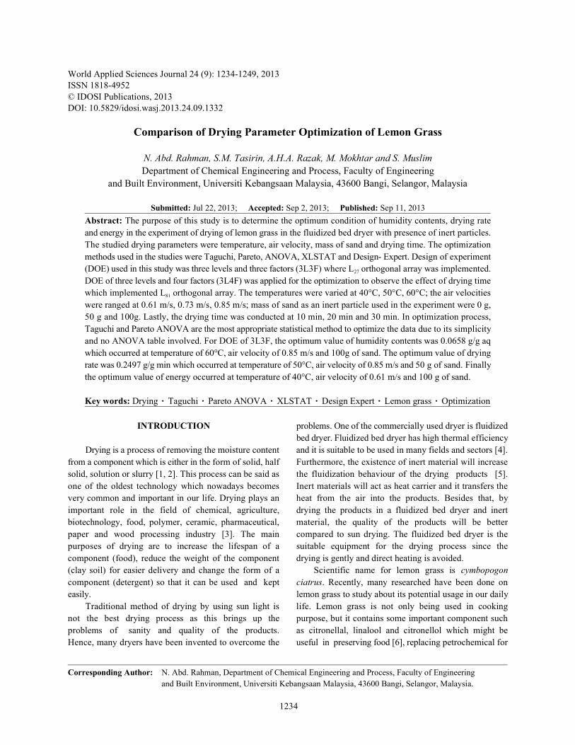
Fluidized Bed Dryer: Lemon grass applies in this dryingexperiment must were cut off and sliced in same size andkept in a container. Lemon grass average size applies inthis experiment were cut into 3 mm x 5 mm in shape andkept in the refrigerator before the experiment wascarried out. The weight of leaves used for each run is 50 Fig. 1: Fluidized bed bin quick dryerg. Sand as the inert particles used has size of 109 µm anddensity of 1968.14 kg/m . Sand applies in this experiment3

is sand from Geldart group particle, A.

Equipment: Fluidized bed bin quick dryer (Model TG 100,Retsch GmbH & Co., Germany) as shown in Fig. 1 wasused for the experiment. This fluidized bed is cylindrical inshape, approximately 18 cm in diameter and 22 cm high,with a voltage of 230 V 50 Hz. Chrome Meter CR-400 isused for the colorimetric testing on the leaves.

Before starting the experiment, the dryer will beturned on for 10 minutes to warm it up. The experiment willbe carried out at different temperature, air velocity, massof sand and drying time. After every 2 minutes of drying,the leaves are weighed and the run is repeated until anearly steady reading is achieved. The leaves will besieved out and separated from the sand by using sievewhen the weight of the leaves is taken. This is to preventthe sand from disturbing the result since a smallportion of sand loses to the environment during the run.Moisture content lost will be calculated using formula thathas been stated in calculation method. Table 1 shows theoperating parameters for lemongrass.

Optimization MethodsDesign of Experiment (DOE): In the optimization process,appropriate selection on DOE is important before theanalysis. For three levels and three factors, a standard L27

orthogonal array is chosen. This orthogonal array ischosen due to its minimum number of experiment trials.The experiment trial is represented by each row in thematrix. Meanwhile for three levels and four factors, astandard of L orthogonal array is chosen.81

Table 1: Operation Parameter for lemongrassExperiment Temperature, Air velocity, Mass ratio, Drying timeset oC m/s 1:X (min)A1 40 0.61 None 30A2 40 0.61 1 30A3 40 0.61 2 30A4 40 0.73 None 30A5 40 0.73 1 30A6 40 0.73 2 30A7 40 0.85 None 30A8 40 0.85 1 30A9 40 0.85 2 30A10 50 0.61 None 30A11 50 0.61 1 30A12 50 0.61 2 30A13 50 0.73 None 30A14 50 0.73 1 30A15 50 0.73 2 30A16 50 0.85 None 30A17 50 0.85 1 30A18 50 0.85 2 30A19 60 0.61 None 30A20 60 0.61 1 30A21 60 0.61 2 30A22 60 0.73 None 30A23 60 0.73 1 30A24 60 0.73 2 30A25 60 0.85 None 30A26 60 0.85 1 30A27 60 0.85 2 30

Taguchi Method: Only ‘the smaller the better’ and ‘thebigger the better’ are applicable in optimization ofhumidity contents and drying rate respectively. This isthe simple method which is no ANOVA table and F-test.Table 2 shows the optimizations method for lemongrass.

2

1

1/ 10logn

ii

S N yn =

= − ∑

10 21

1 1/ 10logn

iiS N

n y=

= − ∑

( ) ( ) ( )2 2 20 1 0 2 1 2AS A A A A A A= − + − + −

Contribution Ratio (%) 100%A

T

SS

= ×

World Appl. Sci. J., 24 (9): 1234-1249, 2013

1236

Table 2: Moisture content for drying of LemongrassExperiment set Temperature, oC Air velocity, m/s Mass ratio, 1:X Drying time (min) Moisture content, X (g/g ak) A1 40 0.61 None 30 1.2162A2 40 0.61 1 30 0.3050A3 40 0.61 2 30 0.1430A4 40 0.73 None 30 0.8142A5 40 0.73 1 30 0.3158A6 40 0.73 2 30 0.1696A7 40 0.85 None 30 0.4122A8 40 0.85 1 30 0.3266A9 40 0.85 2 30 0.1962A10 50 0.61 None 30 0.8875A11 50 0.61 1 30 0.2343A12 50 0.61 2 30 0.1189A13 50 0.73 None 30 0.6075A14 50 0.73 1 30 0.2590A15 50 0.73 2 30 0.1249A16 50 0.85 None 30 0.3274A17 50 0.85 1 30 0.2838A18 50 0.85 2 30 0.1310A19 60 0.61 None 30 0.5588A20 60 0.61 1 30 0.1635A21 60 0.61 2 30 0.0947A22 60 0.73 None 30 0.4007A23 60 0.73 1 30 0.2023A24 60 0.73 2 30 0.0803A25 60 0.85 None 30 0.2426A26 60 0.85 1 30 0.2410A27 60 0.85 2 30 0.0658

For criterion of ‘the smaller the better’, the the value of squares of difference (S) for each factor.formula used to calculate Signal-Noise (SN) ratio to For instance, the formula of sum of squares of differenceminimize humidity contents and energy is shown below for factor A (S ) is depicted below [12].[10]:

(1) After obtaining values of sum of squares of

where y is the independent variable and n is the can be determined by using the formula below [13].i

number of replicates. Meanwhile, ‘the biggerthe better’ criterion used to calculateSN ratio to maximize drying rate is depicted below (4)[11]:

for all factors, the pareto diagram can be constructed in(2) order to observe the major significant effect contributor

In the plot of Taguchi, the level which gives the made from this analysis and it validates the result ofhighest value of sum of SN ratio is the optimum value for optimum condition obtained from Taguchi.that factor.

Pareto ANOVA: Pareto ANOVA analysis is actually regression analysis by XLSTAT, the type of model ofprolonged from Taguchi method where it uses the equation which fits on the experimental data need to bepreviously calculated of sum of SN ratio for all factors at determined. Second-order polynomial model is used aseach level. The next step in this method is to calculate prediction model as shown below [12].

A

(3)

difference for all factors, contribution ratio for al factors

By using the calculated values of contribution ratio

on the dependent variables such as humidity contents,drying rate and energy. Therefore, final conclusion can be

Regression Analysis by XLSTAT: Before performing

12

01 1 1 2

k k k k

i i ii i ij i ji i i j

i j

Y x x x x−

= = = =<

= + + +∑ ∑ ∑∑

World Appl. Sci. J., 24 (9): 1234-1249, 2013

1237

Response Surface Method (RSM) give easily view of(5) response surfaces from all angles with rotatable 3D plots,

where Y is response (humidity contents, drying rate andenergy) and X is independent variables, i, influencing the RESULTS AND DISCUSSIONi

responses Y. X is independent variables, j, influencingj

the responses Y. is regression coefficient of variables The fractional factorial designs used L orthogonal0

for intercept while is regression coefficient of variables array for three levels and three factors and L81 orthogonali

for linear. is regression coefficient of variables for array for three levels and four factors. Levels for eachii

quadratic and is regression coefficient of variables for factor in the matrix were represented by ‘0’, ‘1’ and ‘2’ij

interaction meanwhile k is number of variables. where ‘0’ is the minimum value and ‘2’ is the maximumAlso before performing regression by XLSTAT, the value. Table 3 shows three levels and three factors and

model terms in second-order polynomial model have to be Table 4 shows three factors and four levels used in thiscalculated first. For DOE of three levels and three factors, experiment.model terms such as ‘AB’, ‘AC’, ‘BC’, ‘A ’, ‘B ’ and ‘C ’2 2 2

need to be calculated where the model terms of ‘A’, ‘B’ Taguchi Method: Taguchi method is one of commonand ‘C’ are temperature, air velocity and mass of sand optimization tools practiced by industrial engineers andrespectively. Whereas for DOE of three levels and four chemists to maximize yield of product at optimumfactors, model terms of ‘AB’, ‘AC’, ‘AD’, ‘BC’, ‘BD’, ‘CD’, conditions. This method involves in calculation of SN‘A ’, ‘B ’, ‘C ’ and ‘D ’ need to be calculated where ‘D’ is ratio where it has different criteria which are ‘the smaller2 2 2 2

drying time. the better’, ‘the bigger the better’ and ‘nominal is theThe result of regression from XLSTAT show R , best’. In Taguchi, the analysis is simple due to analysis of2

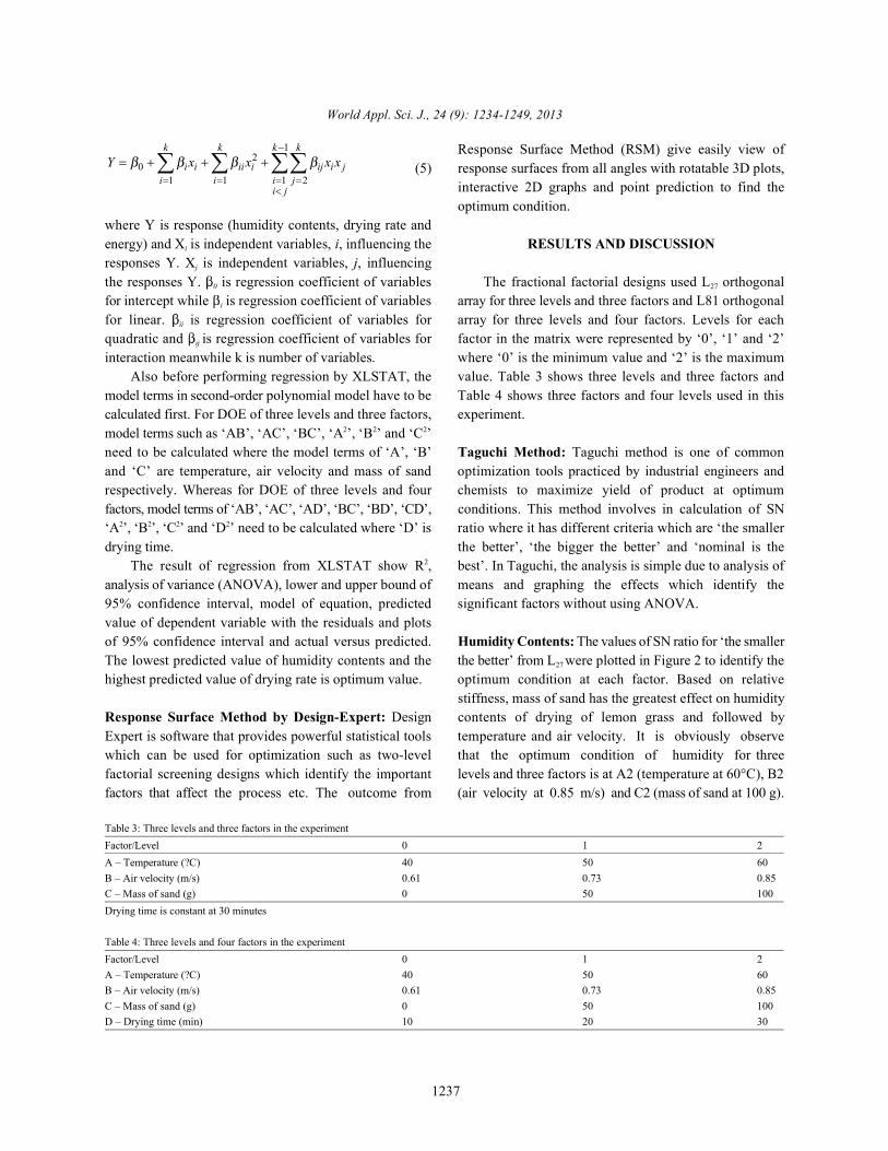
analysis of variance (ANOVA), lower and upper bound of means and graphing the effects which identify the95% confidence interval, model of equation, predicted significant factors without using ANOVA.value of dependent variable with the residuals and plotsof 95% confidence interval and actual versus predicted. Humidity Contents: The values of SN ratio for ‘the smallerThe lowest predicted value of humidity contents and the the better’ from L were plotted in Figure 2 to identify thehighest predicted value of drying rate is optimum value. optimum condition at each factor. Based on relative

Response Surface Method by Design-Expert: Design contents of drying of lemon grass and followed byExpert is software that provides powerful statistical tools temperature and air velocity. It is obviously observewhich can be used for optimization such as two-level that the optimum condition of humidity for threefactorial screening designs which identify the important levels and three factors is at A2 (temperature at 60°C), B2factors that affect the process etc. The outcome from (air velocity at 0.85 m/s) and C2 (mass of sand at 100 g).

interactive 2D graphs and point prediction to find theoptimum condition.

27

27

stiffness, mass of sand has the greatest effect on humidity

Table 3: Three levels and three factors in the experimentFactor/Level 0 1 2A – Temperature (?C) 40 50 60B – Air velocity (m/s) 0.61 0.73 0.85C – Mass of sand (g) 0 50 100Drying time is constant at 30 minutes

Table 4: Three levels and four factors in the experimentFactor/Level 0 1 2A – Temperature (?C) 40 50 60B – Air velocity (m/s) 0.61 0.73 0.85C – Mass of sand (g) 0 50 100D – Drying time (min) 10 20 30

World Appl. Sci. J., 24 (9): 1234-1249, 2013

1238

Fig. 2: Plots of SN Ratio for each drying parameter in determining optimum condition of humidity contents (three levelsand three factors).

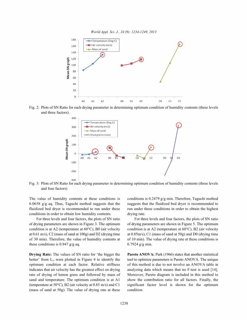
Fig. 3: Plots of SN Ratio for each drying parameter in determining optimum condition of humidity contents (three levelsand four factors)

The value of humidity contents at these conditions is conditions is 0.2479 g/g min. Therefore, Taguchi method0.0658 g/g aq. Thus, Taguchi method suggests that the suggests that the fluidized bed dryer is recommended tofluidized bed dryer is recommended to run under these run under these conditions in order to obtain the highestconditions in order to obtain low humidity contents. drying rate.

For three levels and four factors, the plots of SN ratio For three levels and four factors, the plots of SN ratioof drying parameters are shown in Figure 3. The optimum of drying parameters are shown in Figure 5. The optimumcondition is at A2 (temperature at 60°C), B0 (air velocity condition is at A2 (temperature at 60°C), B2 (air velocityat 0.61 m/s), C2 (mass of sand at 100g) and D2 (drying time at 0.85m/s), C1 (mass of sand at 50g) and D0 (drying timeof 30 min). Therefore, the value of humidity contents at of 10 min). The value of drying rate at these conditions isthese conditions is 0.947 g/g aq. 0.7924 g/g min.

Drying Rate: The values of SN ratio for ‘the bigger the Pareto ANOVA: Park (1966) states that another statisticalbetter’ from L were plotted in Figure 4 to identify the tool to optimize parameters is Pareto ANOVA. The unique27

optimum condition at each factor. Relative stiffness of this method is due to not involve an ANOVA table inindicates that air velocity has the greatest effect on drying analyzing data which means that no F-test is used [14].rate of drying of lemon grass and followed by mass of Moreover, Pareto diagram is included in this method tosand and temperature. The optimum condition is at A1 show the contribution ratio for all factors. Finally, the(temperature at 50°C), B2 (air velocity at 0.85 m/s) and C1 significant factor level is shown for the optimum(mass of sand at 50g). The value of drying rate at these condition.

World Appl. Sci. J., 24 (9): 1234-1249, 2013

1239

Fig. 4: Plots of SN Ratio for each drying parameter in determining optimum condition of drying rate (three levels andthree factors).

Fig. 5: Plots of SN Ratio for each drying parameter in determining optimum condition of drying rate (three levels and fourfactors)

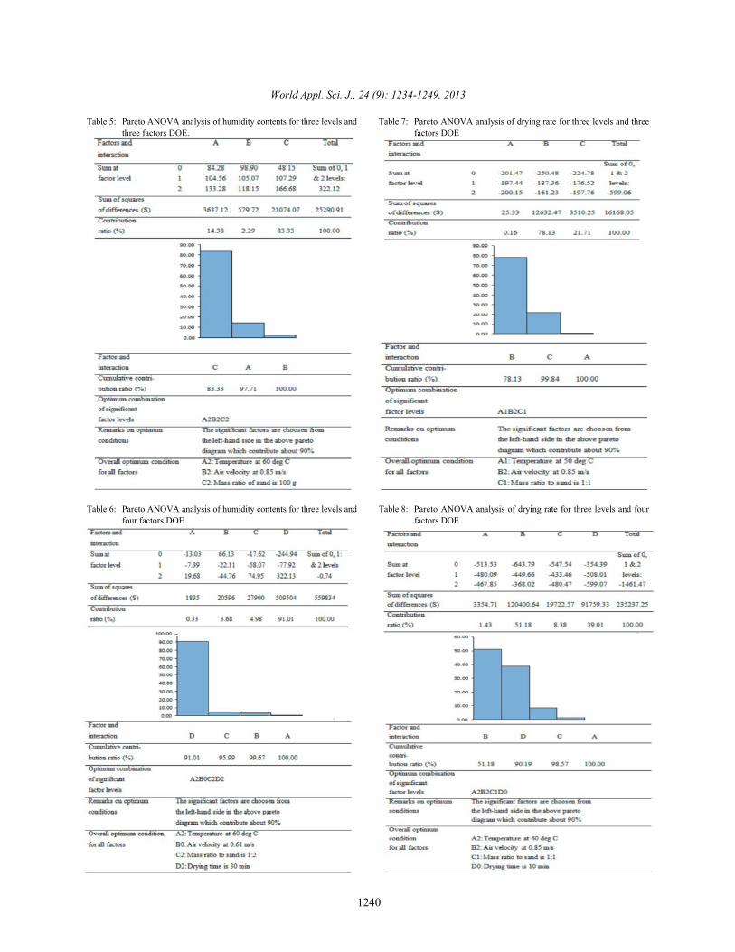
Humidity Contents: Pareto ANOVA analysis of respectively as shown in Table 6. The optimum conditionhumidity contents for three levels and three factors of A2B0C2D2 (temperature of 60°C, air velocity 0.61 m/s,is displayed in Table 5 and shows that mass of sand mass ratio to sand 1:2 and drying time at 30min) isgive the most significant effects where it contributes revealed from Pareto ANOVA analysis was validated83.33% and followed by temperature and air velocity experimentally where the humidity contents was equal towhich contribute 14.38% and 2.29% respectively. The 0.0947 g/g aq.optimum condition of A2B2C2 (temperature of 60°C, airvelocity of 0.85 m/s and mass of sand at 100g) is revealed Drying Rate: Pareto ANOVA analysis of drying ratefrom Pareto ANOVA analysis was validated for three levels and three factors displayed in Table 7experimentally where the humidity contents was equal to shows that air velocity gives the most significant0.0658 g/g aq. effects where it contributes 78.13% and 0.16%

For three levels and four factors, Pareto ANOVA respectively. The optimum condition of A1B2C1analysis of humidity contents shows that drying time (temperature of 50°C, air velocity of 0.85 m/s and massgives the most significant effect where it contributes ration to sand 1:1) is analyzed from Pareto ANOVA91.01% and followed by mass of sand, air velocity and analysis was validated experimentally where the dryingtemperature which contribute 4.98%, 3.68% and 0.33% rate was equal to 0.2497 g/g min.

World Appl. Sci. J., 24 (9): 1234-1249, 2013

1240

Table 5: Pareto ANOVA analysis of humidity contents for three levels and Table 7: Pareto ANOVA analysis of drying rate for three levels and threethree factors DOE. factors DOE

Table 6: Pareto ANOVA analysis of humidity contents for three levels and Table 8: Pareto ANOVA analysis of drying rate for three levels and fourfour factors DOE factors DOE

World Appl. Sci. J., 24 (9): 1234-1249, 2013

1241

For three levels and four factors, Pareto ANOVA Values of Pr>|t| less than 0.0050 shows model termsanalysis of drying rate presented in Table 8 shows that air are significant. In Table 10, model terms such asvelocity gives the most significant effect where it ‘C’,’AC’,’BC’ and ‘C ’ show value of Pr>|t| less thancontributes 51.18% and followed by drying time, mass of 0.0050. This depicts that those model terms are significant.sand and temperature which contribute 39.01%, 8.38% and Whereas the other model terms such as ‘A’,’B’,’AB’,’A ”1.43% respectively. The optimum condition of A2B2C1D0 and ‘B ’ indicate values of Pr>|t| more than 0.1000 which(temperature of 60°C, air velocity of 0.85 m/s, mass ratio to are insignificant model terms. Therefore it can besand 1:1 and drying time of 10 min) is revealed from Pareto concluded that mass of sand gives significant effect forANOVA analysis was proven experimentally where the 3L3F DOE.drying rate was equal to 0.7924 g/g min. The model equation of humidity contents generated

Regression Analysis by XLSTAT: XLSTAT is a softwarepackage which is a part of add-on in EXCEL. In order to Humidity contents = 4.0716 – 0.0418A – 3.4866B –predict a model of equation, regression analysis can (3.4621E – 02)C + (3.2056E – 02)AB + (1.6208E – 04)AC +be performed by XLSTAT using experimental data [15]. (2.3823E – 02)BC – (5.5556E – 08)A – (3.8580E – 04)BPrior to regression analysis, it is essential to determine thetype of model of equation which fits on the experimental From the model of equation, the predicted values ofdata. The second order polynomial model is used in this humidity contents can be calculated and shown incase. Table 11. In row of Observation 12 which is highlighted

Humidity Contents: In Table 9, for 3L3F the degree of humidity contents (0.037 g/g aq). Therefore, the optimumfreedom is 17 and high coefficient of determination (R ) of condition occurs at A1B0C2 which is at temperature of2

0.914 shows that the predicted values were well adapted 50°C, air velocity of 0.61 m/s and mass of sand of 100g.with the experimental data [16]. Both F-test value of 19.949 For 3L4F is shown in Table 12 where the degree ofand value of Pr>F which is less than 0.0050 depict that the freedom is 66 and coefficient of determination (R ) of 0.715model is significant. shows that the predicted values are fairly well adapted

2

2

2

from XLSTAT for 3L3F is shown below:

2 2

with grey shows the smallest value of adjusted predicted

2

Table 9: Goodness of fit statistics and ANOVAGoodness of fit statistics:Observations 27.000Sum of weights 27.000DF 17.000R² 0.914Adjusted R² 0.868Analysis of variance (ANOVA): ...Source DF Sum of squares Mean squares F Pr > F Model 9 1.773 0.197 19.949 < 0.0001 Error 17 0.168 0.010Corrected Total 26 1.941Computed against model Y=Mean(Y)

Table 10: Standardized coefficients for the model terms with t and Pr>|t| valuesSource Value Standard error t Pr > |t| Lower bound (95%) Upper bound (95%) A -1.272 1.350 -0.943 0.359 -4.120 1.575B -1.274 1.569 -0.812 0.428 -4.585 2.037C -5.272 0.734 -7.178 < 0.0001 -6.821 -3.722AB 0.927 0.692 1.341 0.198 -0.532 2.387AC 1.274 0.451 2.825 0.012 0.323 2.226BC 2.709 0.543 4.987 0.000 1.563 3.856A 0.000 1.238 0.000 1.000 -2.611 2.6112

B 0.000 1.505 0.000 1.000 -3.175 3.1752

C 0.679 0.257 2.641 0.017 0.137 1.2222

2 2 2 2

Humidity contents 6.4021 (2.356 02) 12.2118 (1.3209 02) 0.4362

(9.2593 08) (6.4300 04) (5.1446 04) (2.1260 03)(8.7032 02) (3.2282 04) (2.2402 03) (8.8227 02) 0.7309

(

E A B E C D

E A E B E C E DE AB E AC E AD E BC BD

= − − − − − − +

− − − − − − + − +− + − − − + − −

− 6.9081 04)E CD−

World Appl. Sci. J., 24 (9): 1234-1249, 2013

1242

Table 11: Actual humidity contents, predicted value and adjusted predicted value with residual and 95% confidence intervalHumidity Pred (Humidity Std. Std. dev. on Lower bound Upper bound

Observation contents contents) Residual residual pred. (Observation) 95% (Observation) 95% (Observation) Adjusted Pred.Obs1 1.216 1.056 0.160 1.614 0.122 0.798 1.313 0.889Obs2 0.305 0.483 -0.178 -1.794 0.115 0.240 0.726 0.576Obs3 0.143 0.125 0.018 0.180 0.122 -0.132 0.383 0.107Obs4 0.814 0.791 0.023 0.231 0.115 0.548 1.034 0.779Obs5 0.316 0.362 -0.046 -0.463 0.112 0.126 0.597 0.378Obs6 0.170 0.147 0.023 0.231 0.115 -0.096 0.390 0.135Obs7 0.412 0.527 -0.114 -1.151 0.122 0.269 0.784 0.645Obs8 0.327 0.240 0.086 0.869 0.115 -0.003 0.483 0.195Obs9 0.196 0.168 0.028 0.282 0.122 -0.089 0.426 0.139Obs10 0.888 0.834 0.054 0.543 0.115 0.591 1.077 0.805Obs11 0.234 0.342 -0.108 -1.085 0.112 0.107 0.577 0.380Obs12 0.119 0.065 0.054 0.543 0.115 -0.178 0.308 0.037Obs13 0.608 0.607 0.000 0.000 0.112 0.372 0.843 0.607Obs14 0.259 0.259 0.000 0.000 0.112 0.024 0.494 0.259Obs15 0.125 0.125 0.000 0.000 0.112 -0.110 0.360 0.125Obs16 0.327 0.381 -0.054 -0.543 0.115 0.138 0.624 0.409Obs17 0.284 0.176 0.108 1.085 0.112 -0.059 0.411 0.138Obs18 0.131 0.185 -0.054 -0.543 0.115 -0.058 0.428 0.213Obs19 0.559 0.611 -0.053 -0.529 0.122 0.354 0.869 0.666Obs20 0.164 0.201 -0.037 -0.376 0.115 -0.042 0.444 0.220Obs21 0.095 0.005 0.090 0.905 0.122 -0.253 0.262 -0.089Obs22 0.401 0.424 -0.023 -0.231 0.115 0.181 0.667 0.436Obs23 0.202 0.156 0.046 0.463 0.112 -0.079 0.392 0.140Obs24 0.080 0.103 -0.023 -0.231 0.115 -0.140 0.346 0.115Obs25 0.243 0.236 0.007 0.066 0.122 -0.022 0.494 0.229Obs26 0.241 0.112 0.129 1.301 0.115 -0.131 0.355 0.044Obs27 0.066 0.202 -0.136 -1.368 0.122 -0.056 0.459 0.343

Table 12: Goodness of fit statistics and ANOVAGoodness of fit statistics:Observations 81.000Sum of weights 81.000DF 66.000R² 0.715Adjusted R² 0.654Analysis of variance (ANOVA):Source DF Sum of squares Mean squares F Pr > F Model 14 244.739 17.481 11.814 < 0.0001Error 66 97.664 1.480Corrected Total 80 342.403Computed against model Y=Mean(Y)

with the experimental data. Both F-test value of 11.814 and value of Pr>F which is less than 0.0050 indicate that the modelis significant. Table 13 model term such as ‘D’,’BC’,’BD’ and ‘C ’ depicts that those model terms are significant. On the2

other hands, other model such ‘A’,’B’,’C’,’AD’,’CD’,’A ’,’B ’ and ‘D ’ are insignificant. Therefore, it can be concluded2 2 2

that drying time and interactions of ‘mass of sand’, ‘air velocity and mass of sand’ and ‘air velocity and drying time’ givesignificant effect for 3L4F DOE.

The model equation of humidity contents generated from XLSTAT for 3L4F is shown below:

World Appl. Sci. J., 24 (9): 1234-1249, 2013

1243

Table 13: Standardized Coefficients for the model terms with t and Pr>|t| valuesSource Value Standard error t Pr > |t| Lower bound (95%) Upper bound (95%)A -0.094 1.254 -0.075 0.941 -2.598 2.411B 0.582 1.455 0.400 0.691 -2.324 3.488C -0.262 0.696 -0.377 0.707 -1.651 1.127D 1.732 0.788 2.200 0.031 0.160 3.305A 0.000 1.141 0.000 1.000 -2.277 2.2772

B 0.000 1.387 0.000 1.000 -2.769 2.7692

C -1.063 0.237 -4.486 < 0.0001 -1.536 -0.5902

D 0.341 0.460 0.741 0.461 -0.578 1.2602

AB 0.328 0.637 0.515 0.608 -0.944 1.601AC 0.331 0.416 0.796 0.429 -0.499 1.161AD -0.485 0.439 -1.105 0.273 -1.360 0.391BC 1.307 0.501 2.611 0.011 0.308 2.307BD -2.249 0.520 -4.326 < 0.0001 -3.286 -1.211CD -0.327 0.192 -1.704 0.093 -0.709 0.056

Table 14: Actual humidity contents, predicted value and adjusted predicted value with residual and 95% confidence intervalObs46 1.848 3.740 -1.892 -1.555 1.329 1.086 6.394 4.197Obs47 0.820 1.407 -0.587 -0.483 1.298 -1.185 3.999 1.502Obs48 0.327 -0.500 0.828 0.680 1.329 -3.155 2.154 -0.700Obs49 9.027 6.005 3.023 2.485 1.298 3.413 8.597 5.517Obs50 4.397 3.326 1.070 0.880 1.282 0.766 5.887 3.193Obs51 0.284 1.074 -0.790 -0.649 1.298 -1.518 3.665 1.201Obs52 4.660 5.697 -1.037 -0.852 1.329 3.043 8.351 5.947Obs53 2.003 2.673 -0.671 -0.551 1.298 0.082 5.265 2.782Obs54 0.131 0.075 0.056 0.046 1.329 -2.579 2.730 0.062Obs55 1.812 1.590 0.222 0.182 1.375 -1.155 4.336 1.505Obs56 0.913 0.788 0.125 0.103 1.329 -1.867 3.442 0.757Obs57 0.559 0.410 0.149 0.122 1.375 -2.335 3.156 0.353Obs58 1.887 2.958 -1.071 -0.880 1.329 0.303 5.612 3.216Obs59 1.037 1.810 -0.772 -0.635 1.298 -0.782 4.401 1.934Obs60 0.164 1.087 -0.923 -0.759 1.329 -1.568 3.741 1.310Obs61 2.347 1.753 0.595 0.489 1.375 -0.993 4.498 1.524

Table 15: Goodness of fit statistics and ANOVAGoodness of fit statistics:Observations 27.000Sum of weights 27.000DF 17.000R² 0.737Adjusted R² 0.598Analysis of variance (ANOVA):Source DF Sum of squares Mean squares F Pr > F Model 9 0.098 0.011 5.300 0.002Error 17 0.035 0.002Corrected Total 26 0.133Computed against model Y=Mean(Y)

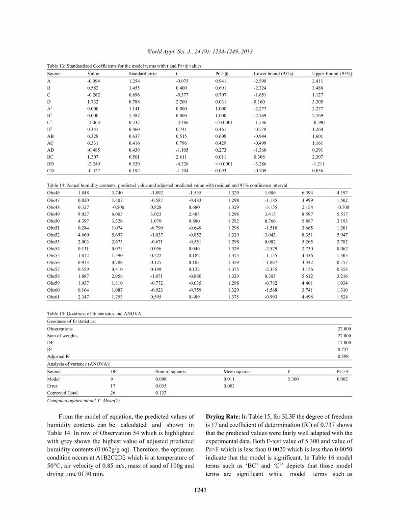
From the model of equation, the predicted values of Drying Rate: In Table 15, for 3L3F the degree of freedomhumidity contents can be calculated and shown in is 17 and coefficient of determination (R ) of 0.737 showsTable 14. In row of Observation 54 which is highlighted that the predicted values were fairly well adapted with thewith grey shows the highest value of adjusted predicted experimental data. Both F-test value of 5.300 and value ofhumidity contents (0.062g/g aq). Therefore, the optimum Pr>F which is less than 0.0020 which is less than 0.0050condition occurs at A1B2C2D2 which is at temperature of indicate that the model is significant. In Table 16 model50°C, air velocity of 0.85 m/s, mass of sand of 100g and terms such as ‘BC’ and ‘C ’ depicts that those modeldrying time 0f 30 min. terms are significant while model terms such as

2

2

World Appl. Sci. J., 24 (9): 1234-1249, 2013

1244

Table 16: Standardized coefficients for the model terms with t and Pr>|t| valuesSource Value Standard error t Pr > |t| Lower bound (95%) Upper bound (95%)A -0.142 2.352 -0.060 0.953 -5.105 4.821B 0.246 2.735 0.090 0.929 -5.525 6.017C -0.957 1.280 -0.747 0.465 -3.657 1.744AB 0.095 1.205 0.078 0.938 -2.449 2.638AC 0.646 0.786 0.822 0.423 -1.013 2.305BC 2.096 0.947 2.214 0.041 0.099 4.094A -0.001 2.157 0.000 1.000 -4.552 4.5502

B 0.000 2.623 0.000 1.000 -5.534 5.5342

C -1.566 0.448 -3.494 0.003 -2.512 -0.6202

Table 17: Actual drying rate predicted value and adjusted predicted value with residual and 95% confidence intervalDrying Pred Std. Std. dev. on Lower bound Upper bound 95%

Observation rate (Drying rate) Residual residual pred. (Observation) 95% (Observation) (Observation) Adjusted Pred.Obs1 0.072 0.040 0.033 0.722 0.056 -0.078 0.157 0.006Obs2 0.028 0.083 -0.055 -1.212 0.052 -0.028 0.194 0.111Obs3 0.019 -0.003 0.022 0.490 0.056 -0.120 0.114 -0.026Obs4 0.078 0.065 0.013 0.286 0.052 -0.046 0.175 0.058Obs5 0.111 0.137 -0.026 -0.572 0.051 0.030 0.244 0.146Obs6 0.093 0.080 0.013 0.286 0.052 -0.030 0.191 0.073Obs7 0.083 0.090 -0.007 -0.150 0.056 -0.027 0.207 0.097Obs8 0.194 0.191 0.003 0.068 0.052 0.080 0.302 0.189Obs9 0.167 0.163 0.004 0.082 0.056 0.046 0.280 0.159Obs10 0.059 0.032 0.026 0.584 0.052 -0.078 0.143 0.019Obs11 0.034 0.087 -0.053 -1.168 0.051 -0.021 0.194 0.105Obs12 0.038 0.012 0.026 0.585 0.052 -0.099 0.122 -0.002Obs13 0.059 0.059 0.000 0.000 0.051 -0.048 0.166 0.059Obs14 0.142 0.142 0.000 0.000 0.051 0.035 0.249 0.142Obs15 0.096 0.096 0.000 0.000 0.051 -0.012 0.203 0.096Obs16 0.059 0.085 -0.026 -0.583 0.052 -0.026 0.196 0.099Obs17 0.250 0.197 0.053 1.168 0.051 0.090 0.304 0.178Obs18 0.153 0.180 -0.026 -0.585 0.052 0.069 0.290 0.193Obs19 0.046 0.025 0.020 0.446 0.056 -0.092 0.143 0.004Obs20 0.039 0.090 -0.051 -1.123 0.052 -0.020 0.201 0.117Obs21 0.057 0.026 0.031 0.677 0.056 -0.091 0.143 -0.006Obs22 0.040 0.053 -0.013 -0.286 0.052 -0.058 0.163 0.059Obs23 0.172 0.146 0.026 0.572 0.051 0.039 0.254 0.137Obs24 0.098 0.111 -0.013 -0.286 0.052 0.000 0.222 0.118Obs25 0.034 0.080 -0.046 -1.018 0.056 -0.037 0.197 0.128Obs26 0.305 0.203 0.103 2.268 0.052 0.092 0.313 0.149Obs27 0.140 0.196 -0.057 -1.249 0.056 0.079 0.313 0.255

Table 18: Goodness of fit statistics and ANOVAGoodness of fit statistics:Observations 81.000Sum of weights 81.000DF 66.000R² 0.818Adjusted R² 0.779Analysis of variance (ANOVA):Source DF Sum of squares Mean squares F Pr > FModel 14 1.442 0.103 21.166 < 0.0001Error 66 0.321 0.005Corrected Total 80 1.763Computed against model Y=Mean(Y)

2 2

Drying Rate 0.0397 (1.218 03) 0.1757 (1.6415 03) (8.541 04)

(2.1475 05) (4.8208 02) (8.3333 08) (2.5823 04)

E A B E C E AB

E AC E BC E A E C

= − − − − − − − + −

+ − + − − − − −

2 2 2 2

Drying Rate 0.6662 (1.5496 03) 1.4348 (2.6442 03) (1.0867 02)

(1.1111 07) (3.858 04) (3.5369 05) (5.2411 04)(3.3333 04) (3.4133 05) (7.5389 05) (7.7167 03)

(4.9650 02

E A B E C E D

E A E B E C E DE AB E AC E AD E BC

E

= − − − − − − + −

− − − − − − + − +− + − − − + −

− − ) (2.7367 05)BD E CD− −

World Appl. Sci. J., 24 (9): 1234-1249, 2013

1245

Table 19: Standardized coefficients for the model terms with t and Pr>|t| values

Source Value Standard error t Pr > |t| Lower bound (95%) Upper bound (95%)

A 0.086 1.002 0.086 0.932 -1.915 2.087B 0.953 1.163 0.819 0.416 -1.369 3.275C -0.732 0.556 -1.316 0.193 -1.842 0.378D 0.601 0.629 0.956 0.343 -0.655 1.858A -0.001 0.911 -0.001 0.999 -1.820 1.8192

B 0.000 1.108 0.000 1.000 -2.213 2.2132

C -1.019 0.189 -5.378 < 0.0001 -1.397 -0.6412

D 1.195 0.368 3.249 0.002 0.460 1.9292

AB -0.018 0.509 -0.034 0.973 -1.035 0.999AC 0.488 0.332 1.468 0.147 -0.176 1.151AD -0.227 0.350 -0.648 0.519 -0.927 0.472BC 1.594 0.400 3.983 0.000 0.795 2.392BD -2.129 0.415 -5.125 < 0.0001 -2.958 -1.299CD -0.180 0.153 -1.177 0.243 -0.486 0.126

‘A’,’B’,’C’,’AB’,’AC’,’A ’ and ‘B ’ are insignificant. Therefore, it can be concluded that interactions of ‘mass of sand’2 2

and ‘air velocity and mass of sand’ give significant effect 3L3F DOE. The model equation of drying rate generated fromXLSTAT for 3L4F is shown below:

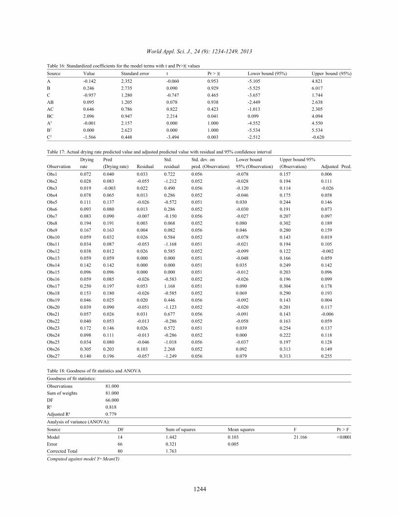
From the model of equation, the predicted values of drying rate can be calculated and shown in Table 17. In row ofObservation 27 which is highlighted with grey shows the highest value of adjusted predicted drying rate (0.255 g/g min).Therefore, the optimum condition occurs at A2B2C2 which is at temperature of 60°C, air velocity of 0.85 m/s and massof sand of 100g.

For 3L4F is shown in Table 18 where the degree of freedom is 66 and coefficient of determination (R ) of 0.818 shows2

that the predicted values were well adapted with the experimental data. Both F-test value of 21.166 and value of Pr>Fwhich is less than 0.0050 indicate that the model is significant. Table 19 model term such as ’BC’,’BD’,’D ’ and ‘C ’2 2

depicts that those model terms are significant. On the other hands, other model such‘A’,’B’,’C’,’D’,’AB’,’AC’,’AD’,’CD’,’A ’ and ’B ’ are insignificant. Therefore, it can be concluded that interactions2 2

between ‘air velocity and mass of sand’, ‘air velocity and drying time’, ‘mass of sand’ and ‘drying time’ give significanteffect for 3L4F DOE.

The model equation of humidity contents generated from XLSTAT for 3L4F is shown below:

From the model of equation, the predicted values of drying rate can be calculated and shown in Table 20. In rowof Observation 79 which is highlighted with grey shows the highest value of adjusted predicted drying rate (0.578).Therefore, the optimum condition occurs at A2B2C2D0 which is at temperature of 60°C, air velocity of 0.85 m/s, mass ofsand of 100g and drying time 0f 10 min.

Response Surface by Design-Expert: Design-Expert is one of the advanced optimization software owned by Stat-EaseInc. In Minneapolis, USA . Design-Expert help the user to analyze the data by providing the outcomes such as a model,graph correlation, ANOVA, diagnostic plots and point prediction of optimization [17].

World Appl. Sci. J., 24 (9): 1234-1249, 2013

1246

Table 20: Actual drying rate predicted value and adjusted predicted value with residual and 95% confidence intervalObs62 0.108 0.027 0.081 1.160 0.076 -0.125 0.179 0.007Obs63 0.057 0.027 0.030 0.425 0.079 -0.130 0.184 0.016Obs64 0.154 0.213 -0.060 -0.854 0.076 0.061 0.366 0.228Obs65 0.082 0.075 0.008 0.109 0.074 -0.074 0.223 0.073Obs66 0.040 0.043 -0.003 -0.042 0.076 -0.110 0.195 0.043Obs67 0.449 0.363 0.086 1.237 0.074 0.214 0.512 0.349Obs68 0.227 0.211 0.016 0.234 0.074 0.064 0.357 0.209Obs69 0.172 0.165 0.007 0.104 0.074 0.016 0.314 0.164Obs70 0.301 0.336 -0.035 -0.498 0.076 0.184 0.488 0.344Obs71 0.162 0.170 -0.008 -0.111 0.074 0.021 0.318 0.171Obs72 0.098 0.111 -0.012 -0.178 0.076 -0.042 0.263 0.114Obs73 0.183 0.324 -0.141 -2.019 0.079 0.166 0.481 0.378Obs74 0.077 0.125 -0.048 -0.692 0.076 -0.027 0.277 0.137Obs75 0.034 0.034 0.000 0.003 0.079 -0.124 0.191 0.034Obs76 0.792 0.520 0.273 3.912 0.076 0.367 0.672 0.454Obs77 0.374 0.308 0.066 0.949 0.074 0.159 0.456 0.297Obs78 0.305 0.202 0.103 1.476 0.076 0.050 0.354 0.177Obs79 0.437 0.539 -0.102 -1.466 0.079 0.381 0.696 0.578Obs80 0.217 0.313 -0.096 -1.382 0.076 0.161 0.465 0.336Obs81 0.140 0.194 -0.055 -0.781 0.079 0.037 0.352 0.215

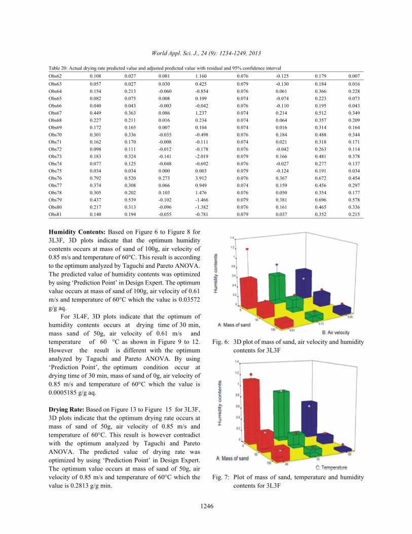
Humidity Contents: Based on Figure 6 to Figure 8 for3L3F, 3D plots indicate that the optimum humiditycontents occurs at mass of sand of 100g, air velocity of0.85 m/s and temperature of 60°C. This result is accordingto the optimum analyzed by Taguchi and Pareto ANOVA.The predicted value of humidity contents was optimizedby using ‘Prediction Point’ in Design Expert. The optimumvalue occurs at mass of sand of 100g, air velocity of 0.61m/s and temperature of 60°C which the value is 0.03572g/g aq.

For 3L4F, 3D plots indicate that the optimum ofhumidity contents occurs at drying time of 30 min,mass sand of 50g, air velocity of 0.61 m/s andtemperature of 60 °C as shown in Figure 9 to 12. Fig. 6: 3D plot of mass of sand, air velocity and humidityHowever the result is different with the optimum contents for 3L3Fanalyzed by Taguchi and Pareto ANOVA. By using‘Prediction Point’, the optimum condition occur atdrying time of 30 min, mass of sand of 0g, air velocity of0.85 m/s and temperature of 60°C which the value is0.0005185 g/g aq.

Drying Rate: Based on Figure 13 to Figure 15 for 3L3F,3D plots indicate that the optimum drying rate occurs atmass of sand of 50g, air velocity of 0.85 m/s andtemperature of 60°C. This result is however contradictwith the optimum analyzed by Taguchi and ParetoANOVA. The predicted value of drying rate wasoptimized by using ‘Prediction Point’ in Design Expert.The optimum value occurs at mass of sand of 50g, airvelocity of 0.85 m/s and temperature of 60°C which the Fig. 7: Plot of mass of sand, temperature and humidityvalue is 0.2813 g/g min. contents for 3L3F

World Appl. Sci. J., 24 (9): 1234-1249, 2013

1247

Fig. 8: 3D plot of temperature, air velocity and humidity Fig. 13:3D plot of mass of sand, air velocity and dryingcontents for 3L3F rate for 3L3F

Fig. 9: 3D plot mass of sand, drying time and humiditycontents for 3L4F Fig. 14:3D plot of mass of sand, temperature and drying

Fig. 10:3D plot mass of drying time, air velocity andhumidity contents for 3L4F Fig. 15:3D plot of temperature, air velocity and drying

Fig. 11:3D plot mass of mass of sand, air velocity and Fig. 16:3D plot of drying time, mass of sand and dryinghumidity contents for 3L4F rate for 3L4F

Fig. 12:3D plot of temperature, mass of sand and Fig. 17:3D plot of dying time, air velocity and drying ratehumidity contents for 3L4 for 3L4F

rate for 3L3F

rate for 3L3F

World Appl. Sci. J., 24 (9): 1234-1249, 2013

1248

Fig. 18:3D plot of mass of sand, air velocity and dryingrate for 3L4F

Fig. 19:3D plot of mass of sand, temperature and dryingrate for 3L4F

For 3L4F, 3D plots indicate that the optimum ofdrying rate occurs at drying time of 10 min, mass sand of50g, air velocity of 0.85 m/s and temperature of 60°C asshown in Figure 16 to 19. The result is similar with theoptimum analyzed by Taguchi and Pareto ANOVA. Byusing ‘Prediction Point’, the optimum condition occur atdrying time of 10 min, mass of sand of 50g, air velocity of0.85 m/s and temperature of 60°C which the value is 0.7770g/g min.

CONCLUSION

The optimization analysis on humidity contents,drying rate and energy for both DOE of 3L3F and 3L4F byusing Taguchi, Pareto ANOVA, XLSTAT and Design-Expert gave different results of optimum condition. Bothconceptual optimization methods which are Taguchi andPareto ANOVA lead to an equal conclusion. However,results of optimization analyzed by XLSTAT and Design-Expert do not agree with the conclusion draw by Taguchiand Pareto ANOVA. The difference of optimization resultsbetween conceptual statistical methods (Taguchi andPareto ANOVA) and statistical software (XLSTAT andDesign Expert) is due to the selection of data foroptimization process. In Taguchi and Pareto ANOVA,experimental data was used which was then converted toSN ratio values. On the other hands, XLSTAT andDesign-Expert developed adjusted predicted values fromgenerated model in determining optimum conditioninstead of using experimental data.

ACKNOWLEDGEMENTS

The research was funded by the UniversitiKebangsaan Malaysia, UKM (UKM-GGPM-2012-072)which is duly acknowledged by the authors.

REFERENCES

1. Seader, J.D. and E.J. Henley, 2006. Separation processprinciples. Ed. ke-2. Asia: John Wiley & Sons PteLtd.

2. Fereydoun Keshavarzpou. 2011. Prediction of CarrotTotal Soluble Solids Based on Water Content andFirmness of Carrot. Agricultural EngineeringResearch Journal, 1(3): 55-58.

3. Mahamud, J.A., M.M. Haque and M. Hasanuzzaman,2013. Growth, Dry Matter Production and YieldPerformance of Transplanted Aman Rice VarietiesInfluenced by Seedling Densities per Hill.International Journal of Sustainable Agriculture,5(1): 16-24.

4. Mujumdar, A.S., 2008. Guide to industrial drying:principles, equipments & new developments.Hyderabad: three S colors

5. Yang, W.C., 2003. Handbook of Fluidization andFluid-Particle Systems. Pennsylvania, USA: MarcelDekker

6. Souraki, B.A. and D. Mowla, 2008. Simulation ofdrying behavior of a small spherical foodstuff in amicrowave assisted fluidized bed of inert particles.Food Research International, 41: 255-265.

7. Jaroenkit, P., N. Matan and M. Nisoa, 2011. In vitroand in vivo activity of citronella oil for the control ofspoilage bacteria of semi dried round scad(Decapterusmaruadsi). Int. J. Med. Arom. Plants,ISSN 2249-4340 1(3):234-239.

8. Lenardao, E.J., V. Botteselle, F. Azambuja, G. Perinand R.G. Jacob, 2007.Citronellal as key compound inorganic synthesis. Tetrahedron, 63: 6671-6712.

9. Chueahongthong, F., C. Ampasavate, S. Okonogi,S. Tima and S. Anuchapreeda, 2011. Cytotoxic effectsof crude kaffir lime (Citrus Hystrix, DC.) leaf fractionalextracts on leukemic cell lines. J. Medicinal PlantsResearch, 5(14): 3097-3105.

10. Fan, S.L., R.M. Awang, D. Omar and M. Rahmani,2011. Insecticidal properties of Citrus hystrix DCleaves essential oil against Spodopteraliturafabricius.J. Medicinal Plants Research, 5(16): 3739-3744.

11. Islam, M.N., Member, Iaeng and B. Boswell, 2011. AnInvestigation of surface finish in dry turning.Proceedings of the World Congress on Engineering,Vol I.

World Appl. Sci. J., 24 (9): 1234-1249, 2013

1249

12. Yusof, F., M. Hameedullah and M. Hamdi, 2006. 15. Tasirin, S.M., S.K.J.A. Kamarudin and K.K. Lee, 2007.Optimization of control parameters for self-lubricating Optimization drying parameters of bird’s eye chilli incharacteristics in a tin base composite. Engineering a fluidized bed dryer. Journal of Food Engineering,e-Transaction, University of Malaya, 1: 19-26. 80: 695-700.

13. Abdullah, H., J. Jurait, A. Lennie, Z.M. Nopiah and 16. Ven, C.V.D., H. Gruppen, D.B.A. Bont andI. Ahmad, 2009. Simulation of fabrication process A.G.J. Voragen, 2002. Optimization of the angiotensinVDMOSFET transistor using Silvaco Software. converting enzyme inhibition by where proteinEuropean Journal of Scientific Research, 29(4). hydrolysates using response surface methodology.

14. Uma, D.B., HO*, C.W. and W.M. Wan Aida, 2010. International Dairy Journal, 12: 813-820.Optimization of Extraction Parameters of Total 17. Wahid, Z. and N. Nadir, 2013. Improvement of OnePhenolic Compounds from Henna (Lawsonia Factor at a Time Through Design of Experiments. orldinermis) Leaves. Sains Malaysiana, 39(1): 119-128. Applied Sciences Journal, 21(Mathematical

Applications in Engineering): 56-61.