comparison of different impulse response measurement techniques
TRANSCRIPT

Comparison of different impulse response measurement techniques
STAN Guy-Bart, EMBRECHTS Jean-Jacques, ARCHAMBEAU Dominique
December 2002
Sound and Image Department, University of Liege, Institut Montefiore B28, Sart Tilman, B-4000 LIEGE 1BELGIUM
Abstract
The impulse response of an acoustical space or transducer is one of their most important characterization. Inorder to perform the measurement of their impulse responses, four of the most suited methods are compared :MLS (Maximum Length Sequence), IRS (Inverse Repeated Sequence), Time-Stretched Pulses and SineSweep.These different methods have already been described in the literature. Nevertheless, the choice of one of thesemethods depending on the measurement conditions is critical. Therefore, an extensive comparison has beenrealized. This comparison has been done through the implementation and realization of a complete, fast, reliableand cheap measurement system. Finally, a conclusion for the use of each method according to the principalmeasurment conditions is presented. It is shown that in the presence of non white noise, the MLS and IRStechniques seem to be more accurate. On the contrary, in quiet environments the Logarithmic SineSweepmethod seems to be the most appropriate.
1 Introduction
Under the assumption of source and receiver immobility, the acoustical space in which they are placed can beconsidered as a Linear and Time Invariant system characterized by an impulse response h(t). In room acoustics,the accurate measurement of the impulse response is very important, since many acoustical parameters can bederived from it. Moreover, in nowadays audio applications (i.e. virtual reality, auralization, spatialization ofsounds), the importance of measuring binaural room impulse responses with a very high signal-to-noise ratiobecomes more and more evident. Once the impulse response has been measured precisely, it can be integratedin a complete auralization process ([1], [2]). In order to achieve the best quality for this auralization process,the measured impulse response must reach a very good signal-to-noise ratio (more than 80 dB if possible).
A common method for measuring the impulse response of such an acoustical system is to apply a known inputsignal and to measure the system’s output. The choice concerning the excitation signal and the deconvolutiontechnique enabling the obtention of the impulse response from the measured output is of essential importance :
• The emitted signal must be perfectly reproducible.
• The excitation signal and the deconvolution technique have to maximize the signal-to-noise ratio of thedeconvolved impulse response.
• The excitation signal and the deconvolution technique must enable the elimination of non linear artifactsin the deconvolved impulse response.
In general, the signal-to-noise ratio is improved by taking multiple averages of the measured output signal beforethe impulse response deconvolution process is started.
The most commonly used excitation signals are deterministic, wide-band signals known as :
• MLS (Maximum Length Sequence) and IRS (Inverse Repeated Sequence) which use pseudo-random whitenoise.
• Time-Streched Pulses and SineSweep which use time varying frequency signals.
1

2 Brief description of the four measurement techniques
The acoustical impulse response measurements using the MLS technique were first proposed by Schroeder in1979 ([3]) and have been used for more than twenty years. Many papers discussed its theoretical and practicaladvantages and inconvenients ([4], [5], [6], [7], [8], [9], [10], [11], [12], [13], [14], [15]). Shortly after the paper ofSchroeder, the IRS thechnique was proposed as an alternative allowing a theoritical reduction of the distortionartifacts introduced by the MLS technique ([4], [16], [17]).
Two years after the proposition of Schroeder, Aoshima introduced a new idea for the measurements ofimpulse responses which led to the time-stretched pulses technique ([18]). His idea was then pushed further inthe paper of suzuki et al. ([19]) proposing what they called an “Optimum computer-generated pulse signal”.
Recently, Farina introduced the logarithmic SineSweep technique ([20], [21]) intended to overcome mostof the limitations encountered in the other techniques. The idea of using a sweep in order to deconvolve theimpulse response is not new ([22]) but the deconvolution method used is different in the paper of Farina.
These techniques have already been described and discussed in many papers. However, it is intended here tofocus on some important properties which are necessary to understand the comparison of the different methods.
2.1 MLS Technique
The MLS technique is based upon the excitation of the acoustical space by a periodic pseudo-random signalhaving almost the same stochastic properties as a pure white noise. The number of samples of one period of anm order MLS signal is: L = 2m − 1.
More theoretical considerations about the MLS sequences can be found in : [7], [10], [12], [13], [23] and inthe excellent book on the shift-register theory [24].
With the MLS technique, the impulse response is obtained by circular cross-correlation (as shown in[25]) between the measured output and the determined input (MLS sequence). Because of the use of circularoperations to deconvolve the impulse response, the MLS technique delivers the periodic impulse response h′[n]which is related to the linear impulse response by the following equation :
h′[n] =
+∞∑
l=−∞
h[n + lL] (1)
Equation (1) reflects the well known problem of the MLS technique : the time-aliasing error. This error issignificant if the length L of one period is shorter than the length of the impulse response to be measured.Therefore, the order m of the MLS sequence must be high enough in order to overcome the time-aliasing error.Our measurement system allows generation of MLS sequences up to order 19 (which corresponds to a period of12 seconds if the sampling frequency is 44.1 kHz).
2.1.1 MLS Immunity to signals not correlated with the excitation signal
Each MLS sequence is characterized by a phase spectrum which is strongly erratic, with a uniform density ofprobability in the [−π , +π] interval as can be seen in figure 1.
According to this property, the MLS technique is able to randomize the phase spectrum of any componentof the output signal which is not correlated with the MLS input sequence ([5], [9]). As a consequence, anydisturbing signal (i.e. white or impulsive noise) will actually be phase randomized, and this will lead to auniform repartition of the disturbing effects along the deconvolved impulse response (see figures 2 and 3)instead of localized noise contributions along the time axis. A post-averaging method can then be used in orderto reduce this uniformly distributed noise appearing in the deconvolved impulse response.
2.1.2 Inconvenients of the MLS technique
The major problem of the MLS method resides in the appearance of distortion artifacts known as “distortionpeaks” ([6]). These artifacts are more or less uniformly distributed along the deconvolved impulse response.The origin of the distortion peaks lies in the non linearities inherent to the measurement system and especiallyto the loudspeaker.
These distortion artifacts introduce characteristic crackling noise when the measured impulse response isconvolved with some anechoic signal in order to realize the auralization process. These distortion peaks can beattenuated by:
• The use of dedicated measurement methods (such as the Inverse Repeated Sequence technique ([4], [16])).
• The optimization of some measurement parameters. For example, the amplitude of the excitation signal is,in practice, a compromise between increasing distortions at high levels and decreasing the signal-to-noiseratio at low levels. This optimization is very time consuming because of the practical difficulty to findthe optimal amplification level. Moreover, this compromise level must be carefully chosen for each newmeasurement situation.
2

Figure 5 illustrates the quality of the results that can be obtained when particular care is taken for the opti-mization of the parameters (mainly the output level) conditioning the MLS (or IRS) input signal. It can beseen that the distortion peaks are significantly reduced but not completely removed.
2.2 IRS technique
Each IRS sequence with a 2L samples period (x[n]) is defined from the corresponding MLS sequence of periodL (mls[n]) by the following relation :
x[n] =
{
mls[n], if n is even, 0 ≤ n < 2L−mls[n], if n is odd, 0 < n < 2L
(2)
The deconvolution process is exactly the same as for the MLS technique (circular correlation).Figure 4 shows the attenuation of the distortion peaks when the IRS method is used. These impulse responses
have been obtained by performing the measurements in an anechoic room leaving all measurement parametersunchanged from one measure to the other.
2.3 Time-Stretched Pulses technique
This method is based on a time expansion and compression technique of an impulsive signal ([18]). Theaim of using an expansion process for the excitation signal is to increase the amount of sound power emittedfor a fixed magnitude of this signal and therefore to increase the signal-to-noise ratio without increasing thenonlinearities introduced by the measurement system. Once the response to this “streched” signal has beenmeasured, a compression filter is used in order to compensate for the induced stretching effects and to obtainthe deconvolved impulse response.
Figure 6 shows the impulse response obtained with this technique. The magnitude scale has been enlargedto clearly illustrate the absence of distortion peaks. However, this does not mean that distortion artifacts arecompletely removed. They still appear in the impulse response (as a residue of the deconvolution filter) as canbe seen on figure 7.
2.4 Logarithmic SineSweep technique
The MLS, IRS and Time-Stretched Pulses methods rely on the assumption of LTI (Linear, Time-Invariant)Systems and cause distortion artifacts to appear in the deconvolved impulse response when this condition is notfullfilled.
The SineSweep technique developed by Farina ([21]) overcomes such limitations. It is based on the followingidea : by using an exponential time-growing frequency sweep, it is possible to simultaneously deconvolve thelinear impulse response of the system and to selectively separate each impulse response corresponding to theharmonic distortion orders considered. The harmonic distortions appear prior to the linear impulse response.Therefore, the linear impulse response measured is assured exempt from any non linearity and, at the sametime, the measurement of the harmonic distortion at various orders can be performed.
Figure 8 illustrates the black box modelization of the measurement process common to all four techniquesdiscussed in this paper. In this modelization it is assumed that the measurement system is intrinsically notlinear but, on the other hand, perfect linearity is considered regarding the acoustical space from which theimpulse response is to be derived.
As pointed out by Farina ([21]), the signal emitted by the loudspeaker is composed of harmonic distortions(considered here without memory) and may be thus represented by the following equation (see figure 8) :
w(t) = x(t) ⊗ k1(t) + x2(t) ⊗ k2(t) + x3(t) ⊗ k3(t) + ... + xN (t) ⊗ kN (t) (3)
where ki(t) represents the ith component of the Volterra Kernel ([21]) which takes into account thenonlinearities of the measurement system.
In practice, it is relatively difficult to separate the linear part (reverberation part in the impulse response)from the non linear part (distortions). In the following, we will consider the response of the global system (theoutput signal from the system represented in figure 8) as being composed of an additive gaussian white noise(n(t)) and a set of impulse responses (hi(t)), each of them being convolved by a different power of the inputsignal.
y(t) = n(t) + x(t) ⊗ h1(t) + x2(t) ⊗ h2(t) + x3(t) ⊗ h3(t) + ... + xN (t) ⊗ hN(t) (4)
where hi(t) = ki(t) ⊗ h(t).Equation (4) underlines the existence of the non linearities at the system’s output.In the case of the logarithmic SineSweep technique, the excitation signal is generated on the basis of the
following equation (see [21] for more theoretical informations) :
3
x(t) = sin
[
Tω1
ln(ω2
ω1
)(e
t
Tln(
ω2
ω1)− 1)
]
(5)
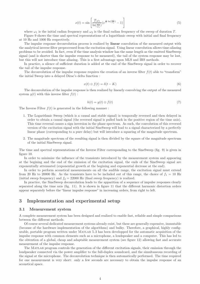
where ω1 is the initial radian frequency and ω2 is the final radian frequency of the sweep of duration T .Figure 9 shows the time and spectral representations of a logarithmic sweep with initial and final frequency
at 10 Hz and 1000 Hz respectively.The impulse response deconvolution process is realized by linear convolution of the measured output with
the analytical inverse filter preprocessed from the excitation signal. Using linear convolution allows time-aliasingproblems to be avoided. In fact, even if the time analysis window has the same length as the emitted SineSweepsignal (and is shorter than the impulse response to be measured), the tail of the system response may be lost,but this will not introduce time aliasing. This is a first advantage upon MLS and IRS methods.
In practice, a silence of sufficient duration is added at the end of the SineSweep signal in order to recoverthe tail of the impulse response.
The deconvolution of the impulse response requires the creation of an inverse filter f(t) able to “transform”the initial Sweep into a delayed Dirac’s delta function :
x(t) ⊗ f(t) = δ(t − K) (6)
The deconvolution of the impulse response is then realized by linearly convolving the output of the measuredsystem y(t) with this inverse filter f(t) :
h(t) = y(t) ⊗ f(t) (7)
The Inverse Filter f(t) is generated in the following manner :
1. The Logarithmic Sweep (which is a causal and stable signal) is temporally reversed and then delayed inorder to obtain a causal signal (the reversed signal is pulled back in the positive region of the time axis).This time reversal causes a sign inversion in the phase spectrum. As such, the convolution of this reversedversion of the excitation signal with the initial SineSweep will lead to a signal characterized by a perfectlylinear phase (corresponding to a pure delay) but will introduce a squaring of the magnitude spectrum.
2. The magnitude spectrum of the resulting signal is then divided by the square of the magnitude spectrumof the initial SineSweep signal.
The time and spectral representations of the Inverse Filter corresponding to the SineSweep (fig. 9) is given infigure 10.
In order to minimize the influence of the transients introduced by the measurement system and appearingat the begining and the end of the emission of the excitation signal, the ends of the SineSweep signal areexponentially attenuated (exponential growth at the begining and exponential decrease at the end).
In order to perform acoustical measurements on all the audible range, the excitation signal must extendfrom 20 Hz to 20000 Hz. As the transients have to be included out of this range, the choice of f1 = 10 Hz(initial sweep frequency) and f2 = 22000 Hz (final sweep frequency) is realized.
In practice, the SineSweep deconvolution leads to the apparition of a sequence of impulse responses clearlyseparated along the time axis (fig. 11). It is shown in figure 11 that the different harmonic distortion ordersappear separately before the “linear impulse response” in increasing orders, from right to left.
3 Implementation and experimental setup
3.1 Measurement system
A complete measurement system has been designed and realized to enable fast, reliable and simple comparisonsbetween the different methods.
Of course several dedicated measurement systems already exist, but these are generally expensive, immutable(because of the hardware implementation of the algorithms) and bulky. Therefore, a graphical, highly config-urable, portable program written under Matlab 5.3 has been developped for the automatic acquisition of theimpulse response with common elements such as a microphone, a loudspeaker and a computer. This has led tothe obtention of a global, cheap and adaptable measurement system (see figure 12) allowing fast and accuratemeasurement of the impulse response.
The Matlab program controls the generation of the different excitation signals, their emission through theloudpseaker connected via the power amplifier to the full-duplex soundcard, and the simultaneous recording ofthe signal at the microphone. The deconvolution technique is then automatically performed. The time requiredfor one measurement is very short: only a few seconds are necessary to obtain the impulse response of anacoustical space.
4

3.2 Room impulse response acquisition
In order to accurately measure room impulse responses, the measurement system characteristics must be takeninto consideration.
The calibration of the whole measurement chain requires an inverse filtering correction which, in this case, isrealized by the application of the “Time Reversal Mirror Filter” technique ([26]). This last technique generatesa pre-equalized excitation signal in three steps :
1. Acquisition of the measurement system impulse response in an anechoic room (for example by using oneof the technique described earlier).
2. time reversal of the system impulse response after appropriate truncation and addition of a time delay inorder to obtain a causal result1. This “reversed” impulse response is linearly convolved with the excitationsignal (MLS, sweep, ...) that has to be pre-equalized.
3. Division of the spectrum magnitude of the signal obtained in step 2 by the square of the measurementsystem magnitude response (Fast Fourier Transform of the impulse response obtained in step 1).
The results of the pre-equalization technique are presented in figure 13. It can be seen that the phase spectrumis perfectly linear and the amplitude spectrum is almost constant (the residual oscillations around the meanvalue do not exceed ±0.4 dB) in the range between 40 Hz and 18 kHz.
4 Comparison of the four methods
The comparison of the four impulse response measurement methods has been first realized in the anechoic roomin order to insure individual control of the set of parameters conditioning the measurement. The characteristicparameters of each method have been chosen in order to allow an objective comparison : for example, theduration of the excitation signals and the number of averages used have been maintained constant during allmeasurements.
The program written under Matlab allows the following parameters to be modified :
Parameters common to all methods :
• sampling frequency
• number of averages (i.e. number of times the emitted signal will be send to the loudspeaker)
• Recording mode : mono or stereo (for example for Head Related Impulse Responses measurements)
Parameters specific to each method :
MLS
Order of the MLS sequence (Maximum order = 19 ; number of samples contained in one period of an m orderMLS sequence=2m − 1)
IRS
Order of the IRS sequence (Maximum order = 19 ; number of samples contained in one period of an m orderIRS sequence=2 ∗ (2m − 1))
Time-Stretched Pulses
• Total duration of the pulse
• Stretching percentage (indication of the ratio between the amount of time during which the pulse has anon negligible amplitude and the total duration of the pulse)
SineSweep
• initial frequency
• final frequency
• sweep duration
• duration of the silences inserted after each sweep
Figure 14 illustrates the disposition of the transducers in the anechoic room in order to compare the differentmeasurement techniques.
1The aim of this step is to inverse the phase polarity of the signal.
5
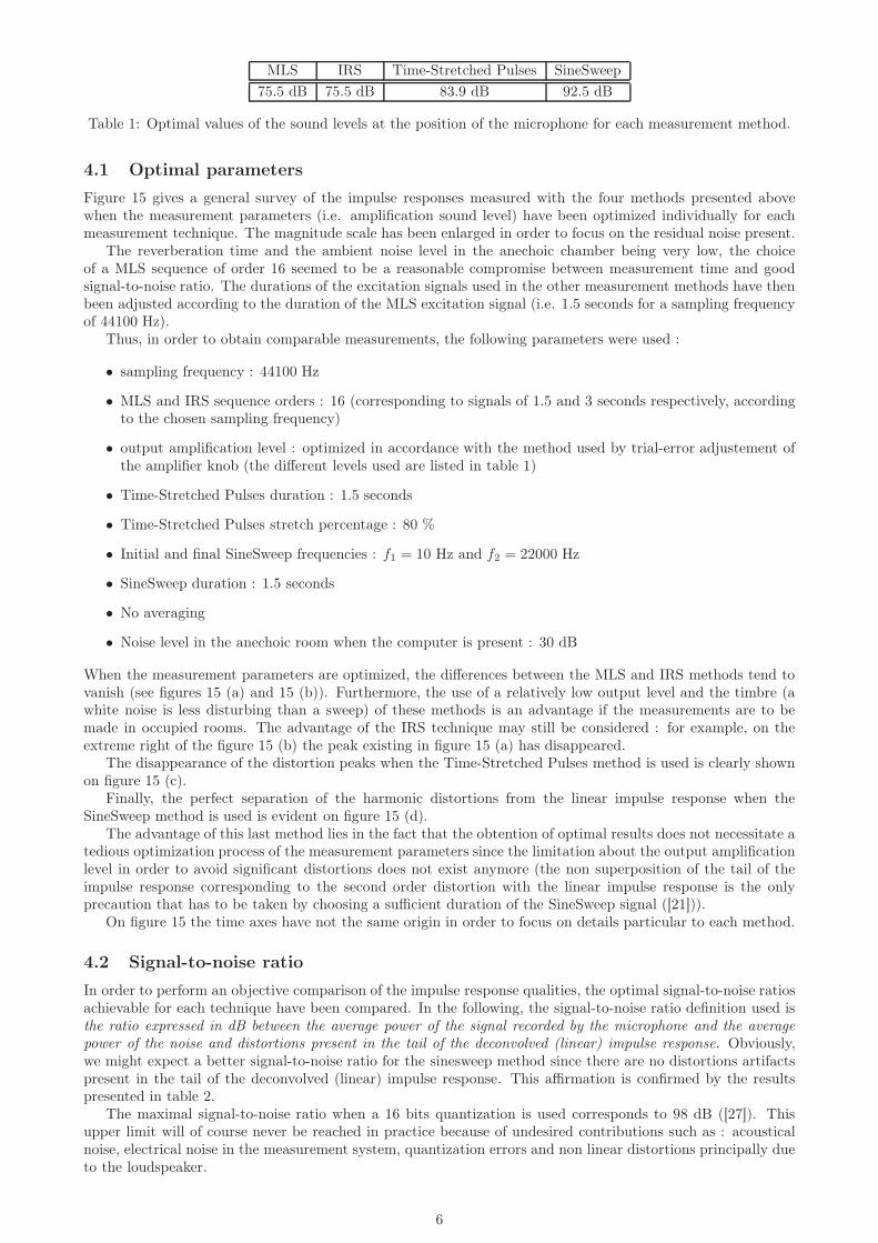
MLS IRS Time-Stretched Pulses SineSweep
75.5 dB 75.5 dB 83.9 dB 92.5 dB
Table 1: Optimal values of the sound levels at the position of the microphone for each measurement method.
4.1 Optimal parameters
Figure 15 gives a general survey of the impulse responses measured with the four methods presented abovewhen the measurement parameters (i.e. amplification sound level) have been optimized individually for eachmeasurement technique. The magnitude scale has been enlarged in order to focus on the residual noise present.
The reverberation time and the ambient noise level in the anechoic chamber being very low, the choiceof a MLS sequence of order 16 seemed to be a reasonable compromise between measurement time and goodsignal-to-noise ratio. The durations of the excitation signals used in the other measurement methods have thenbeen adjusted according to the duration of the MLS excitation signal (i.e. 1.5 seconds for a sampling frequencyof 44100 Hz).
Thus, in order to obtain comparable measurements, the following parameters were used :
• sampling frequency : 44100 Hz
• MLS and IRS sequence orders : 16 (corresponding to signals of 1.5 and 3 seconds respectively, accordingto the chosen sampling frequency)
• output amplification level : optimized in accordance with the method used by trial-error adjustement ofthe amplifier knob (the different levels used are listed in table 1)
• Time-Stretched Pulses duration : 1.5 seconds
• Time-Stretched Pulses stretch percentage : 80 %
• Initial and final SineSweep frequencies : f1 = 10 Hz and f2 = 22000 Hz
• SineSweep duration : 1.5 seconds
• No averaging
• Noise level in the anechoic room when the computer is present : 30 dB
When the measurement parameters are optimized, the differences between the MLS and IRS methods tend tovanish (see figures 15 (a) and 15 (b)). Furthermore, the use of a relatively low output level and the timbre (awhite noise is less disturbing than a sweep) of these methods is an advantage if the measurements are to bemade in occupied rooms. The advantage of the IRS technique may still be considered : for example, on theextreme right of the figure 15 (b) the peak existing in figure 15 (a) has disappeared.
The disappearance of the distortion peaks when the Time-Stretched Pulses method is used is clearly shownon figure 15 (c).
Finally, the perfect separation of the harmonic distortions from the linear impulse response when theSineSweep method is used is evident on figure 15 (d).
The advantage of this last method lies in the fact that the obtention of optimal results does not necessitate atedious optimization process of the measurement parameters since the limitation about the output amplificationlevel in order to avoid significant distortions does not exist anymore (the non superposition of the tail of theimpulse response corresponding to the second order distortion with the linear impulse response is the onlyprecaution that has to be taken by choosing a sufficient duration of the SineSweep signal ([21])).
On figure 15 the time axes have not the same origin in order to focus on details particular to each method.
4.2 Signal-to-noise ratio
In order to perform an objective comparison of the impulse response qualities, the optimal signal-to-noise ratiosachievable for each technique have been compared. In the following, the signal-to-noise ratio definition used isthe ratio expressed in dB between the average power of the signal recorded by the microphone and the averagepower of the noise and distortions present in the tail of the deconvolved (linear) impulse response. Obviously,we might expect a better signal-to-noise ratio for the sinesweep method since there are no distortions artifactspresent in the tail of the deconvolved (linear) impulse response. This affirmation is confirmed by the resultspresented in table 2.
The maximal signal-to-noise ratio when a 16 bits quantization is used corresponds to 98 dB ([27]). Thisupper limit will of course never be reached in practice because of undesired contributions such as : acousticalnoise, electrical noise in the measurement system, quantization errors and non linear distortions principally dueto the loudspeaker.
6

MLS IRS Time-Stretched Pulses SineSweep
60.5 dB 63.2 dB 77.0 dB 80.1 dB
Table 2: Optimal signal-to-noise ratios for each method.
Table 2 shows the optimal signal-to-noise ratios (i.e. the signal-to-noise ratios obtained when the measure-ment parameters have been optimized) for each of the four methods presented above.
Bleakley and Scaife ([11]) have showed that the signal-to-noise ratio for the MLS sequence increases by3dB when the period length of the MLS sequence is doubled. It is thus logical to obtain a 3 dB gain for the IRStechnique in comparison to the MLS since the length of an IRS sequence is twice the length of the corresponding(same order) MLS sequence.
The noticeable gain of 14 dB of the Time-Stretched Pulses method on the IRS method can be explained bythe use of an optimal output sound level far above the one used in the MLS or IRS cases, as well as by thedisappearance of the spurious distortion peaks.
Finally, the excellent signal-to-noise ratio (80 dB) obtained with the SineSweep technique is due to the totalrejection of the non linear distortion artifacts prior to the linear impulse response. The output signal level isnot limited anymore by the need to reduce the non linear influence since all non linear distortions are measuredseparately. This leads to the best optimal signal-to-noise ratio (20 dB better than for the MLS method).This signal-to-noise ratio is only 3 dB above the one given by the Time-Stretched Pulses method, but the nonsuperposition of the distortion artifacts is guaranteed in this case.
All these signal-to-noise ratios have been obtained through direct (no averaging) measurements. Of course,better signal-to-noise ratios would have been obtained if averaging had been used.
4.3 Impulsive noise Immunity
Figure 16 shows the impulse responses obtained when measurements are performed in an environment whereimpulsive noise is simultaneously present. The IRS method gives results approximately identical to those ofthe MLS technique and thus its corresponding impulse response is not shown here. As previously announced,only the pseudo-random noise techniques (MLS and IRS) possess the ability of randomizing the phase of anycomponent in the recorded signal that is not correlated to the input signal emitted in the acoustical space. Thus,any additional noise (white or even impulsive) will be uniformly distributed along the deconvolved impulseresponse. Therefore, additive impulsive noise (appearing as additive white noise in the deconvolved impulseresponse) is subject to posterior attenuation by averaging techniques.
On the contrary, the presence of impulsive noise when the Time-Stretched Pulse or SineSweep techniquesare used, heavily compromises the impulse response deconvolution process through the presence of excitationsignal residues in the deconvolved impulse response. These residues being strongly correlated with the excitationsignal will not be properly eliminated if posterior average techniques are used.
As a first conclusion, we may say that in a (non random) noisy environment, the MLS (IRS) method issubject to give better results than the other two.
4.4 Impulse response measurements in classical rooms
The properties described above were mostly illustrated by measurements performed in anechoic rooms. In thissection we will show the results given when the measurements are performed in more classical rooms such asauditoria or lecture rooms.
As can be seen on figure 18, most of the properties that have been illustrated in the case of anechoicmeasurements are still visible. We can particularly focus on the separation of the different harmonic distortionsfrom the linear impulse response in the case of the SineSweep technique. In this case, the impact of reverberationon each impulse response can be clearly seen and illustrates the need for non superposition of the second orderdistortion with the linear impulse response by using a sufficiently long SineSweep.
5 Conclusions
A complete, cheap and parametrizable measurement system has been realized in order to compare differentimpulse response measurement methods. This system is based on a computer program written under Matlab5.3 allowing an automatic and easy measurement to be realized. On the basis of this measurement system, acomparison of four different methods has been done.
The comparison of the four methods leads us to the following conclusions :
1. The MLS (IRS) method seems the most interesting method when the measurements have to be performedin an occupied room or in exterior due to its strong immunity to all kinds of noise (white, impulsive orothers), its weak optimal output sound level and its timbre (white noise is more supportable and easily
7

masked out than sweep signals). However, its major drawback lies in the tedious calibration that has tobe carried out to obtain optimal results and in the appearance of spurious peaks (“distortion peaks”) dueto the inherent non linearities of the measurement system.
2. The Time-Strectched Pulses method avoids the appearance of the distortion peaks. However, the remain-ing non linear artifacts can possibly be superimposed with the deconvolved “linear” impulse response.The presence of a residue of the excitation signal in the deconvolved impulse response is a result of suchsuperposition problem. This residue can be almost completely eliminated if a precise calibration of themeasurement parameters (mainly the output level) is realized. However, its timbre and the high valueof the optimal output signal level needed to mask out the ambient noise makes it unusable in occupiedrooms.
3. The perfect and complete rejection of the harmonic distortions prior to the “linear” impulse response,their individual measurement and the excellent signal-to-noise ratio of the SineSweep method make it thebest impulse response measurement technique in an inoccupied and quiet room. Moreover, unlike thepreceding methods, it does not necessitate a tedious calibration in order to obtain very good results (nocompromise between the signal-to-noise ratio and the superposition of non linear artifacts in the roomimpulse response). However, as for the Time-Stretched Pulses method, the SineSweep technique is notrecommended for measurements in occupied rooms.
References
[1] M. Kleiner, B.-I. Dalënback, and P. Svensson, “Auralization-an overview,” vol. 41, no. 11, pp. 861–875,1993.
[2] H. Lehnert and J. Blauert, “Principles of binaural room simulation,” Applied Acoustics, vol. 36, pp.259–291, 1992.
[3] M. R. Schroeder, “Integrated-impulse method for measuring sound decay without using impulses,”vol. 66, no. 2, pp. 497–500, 1979.
[4] C. Dunn and M. O. Hawksford, “Distortion immunity of mls-derived impulse response measurements,”vol. 41, no. 5, pp. 314–335, 1993.
[5] D. D. Rife and J. Vanderkooy, “Transfer function measurement with maximum-length sequences,”vol. 37, no. 6, pp. 419–443, 1989.
[6] J. Vanderkooy, “Aspects of mls measuring systems,” vol. 42, no. 4, pp. 219–231, 1994.
[7] H. Alrutz and M. R. Schroeder, “A fast hadamard transform method for the evaluation of mea-surements using pseudorandom test signals,” Proc. 11th Int. Conf. on Acoust., Paris, pp. 235–238,1983.
[8] H. R. Simpson, “Statistical properties of a class of pseudorandom sequences,” Proc. IEEE(London),vol. 133, pp. 2075–2080, 1966.
[9] D. D. Rife, “Modulation transfer function measurement with maximum-length sequences,” vol. 40,no. 10, pp. 779–789, 1992.
[10] J. Borish and J. B. Angell, “An efficient algorithm for measuring the impulse response using pseudo-random noise,” vol. 31, no. 7, pp. 478–487, 1983.
[11] C. Bleakley and R. Scaife, “New formulas for predicting the accuracy of acoustical measurementsmade in noisy environments using the averaged m-sequence correlation technique,” vol. 97, no. 2, pp.1329–1332, 1995.
[12] M. Cohn and A. Lempel, “On fast m-sequence transforms,” IEEE Trans. Inf. Theory, vol. IT-23, pp.135–137, 1977.
[13] W. D. T. Davies, “Generation and properties of maximum-length sequences,” Control, pp. 302–304,364–365, 431–433, 1966.
[14] M. Vorländer and M. Kob, “Practical aspects of mls measurements in building acoustics,” AppliedAcoustics, vol. 52, no. 3/4, pp. 239–258, 1997.
[15] R. Burkard, Y. Shi, and K. E. Hecox, “A comparison of maximum length and legendre sequences forthe derivation of brain-stem auditory-evoked responses at rapid rates of stimulation,” vol. 87, no. 4,pp. 1656–1664, 1990.
[16] N. Ream, “Nonlinear identification using inverse-repeat m sequences,” Proc. IEE(London), vol. 117,pp. 213–218, 1970.
[17] P. A. N. Briggs and K. R. Godfrey, “Pseudorandom signals for the dynamic analysis of multivariablesystems,” Proc. IEEE, vol. 113, pp. 1259–1267, 1966.
8

0 0.5 1 1.5 2 2.5
x 104
0
10
20
30
40
50
60Magnitude
dB
Freq, Hz
1440 1450 1460 1470 1480 1490 1500 1510 1520 1530 1540
−3
−2
−1
0
1
2
3
Phase
radi
ans
Freq, Hz
Figure 1: Magnitude and Phase Spectra of an MLS sequence. The phase spectrum has been enlarged in orderto clearly show its uniform random distribution.
[18] N. Aoshima, “Computer-generated pulse signal applied for sound measurement,” vol. 65, no. 5, pp.1484–1488, 1981.
[19] Y. Suzuki, F. Asano, H.-Y. Kim, and T. Sone, “An optimum computer-generated pulse signal suitablefor the measurement of very long impulse responses,” vol. 97, no. 2, pp. 1119–1123, 1995.
[20] A. Farina and E. Ugolotti, “Subjective comparison between stereo dipole and 3d am-bisonic surround systems for automotive applications (available at the following url :HTTP://pcfarina.eng.unipr.it),” AES 16th International Conference on Spatial Sound Reproduc-tion.
[21] A. Farina, “Simultaneous measurement of impulse response and distorsion with a swept-sine technique(preprint 5093),” Presented at the 108th AES Convention, Paris, France, February 19-22 2000.
[22] A. J. Berkhout, M. M. Boone, and C. Kesselman, “Acoustic impulse response measurement : A newtechnique,” vol. 32, no. 10, pp. 740–746, 1984.
[23] J. Borish, “Self-contained crosscorrelation program for maximum-length sequences,” vol. 33, no. 11,pp. 888–891, 1985.
[24] S. W. Golomb, Shift-Register Sequences. Aegan Park Press, 1982.
[25] A. V. Oppenheim and R. W. Schafer, Discrete-Time Signal Processing, 2nd ed., ser. Prentice HallSignal Processing Series. Prentice Hall, 1999.
[26] D. Preis, “Phase distortion and phase equalization in audio signal processing-a tutorial review,” vol. 30,no. 11, pp. 774–794, 1982.
[27] K. C. Pohlmann, Principles of Digital Audio, 3rd ed. Mc Graw Hill, 1995.
9

0.1 0.2 0.3 0.4 0.5 0.6 0.7
−0.8
−0.6
−0.4
−0.2
0
0.2
0.4
0.6
0.8
Impulse Response
Time, sec.
Am
plitu
de
0.8 0.85 0.9 0.95 1 1.05 1.1
−5
−4
−3
−2
−1
0
1
2
3
4
x 10−3 Impulse Response
Time, sec.
Am
plitu
de
(a) (b)
Figure 2: (a) Impulse response of a classroom obtained with a single MLS sequence of order 18 when a whitenoise generator is simultaneously present. The Noise Level measured at the position of the microphone is 60 dB.(b) Zoom on the end of the impulse response.
0.01 0.02 0.03 0.04 0.05 0.06 0.07
−0.8
−0.6
−0.4
−0.2
0
0.2
0.4
Impulse Response
Time, sec.
Am
plitu
de
0.01 0.02 0.03 0.04 0.05 0.06 0.07−0.04
−0.03
−0.02
−0.01
0
0.01
0.02
0.03
Impulse Response
Time, sec.
Am
plitu
de
(a) (b)
Figure 3: (a) Impulse response obtained with a single MLS sequence of order 16 in an anechoic room whenImpulsive Noise is simultaneously present. (b) Zoom on the magnitude scale.
0 0.05 0.1 0.15 0.2 0.25
−6
−4
−2
0
2
4
6
x 10−3 Impulse response
Time, sec.
Am
plitu
de
0 0.05 0.1 0.15 0.2 0.25
−6
−4
−2
0
2
4
6
x 10−3 Impulse response
Time, sec.
Am
plitu
de
(a) (b)
Figure 4: Zoom on the impulse responses obtained via MLS and IRS methods. (a) MLS method. (b) IRSmethod.
10

0 0.2 0.4 0.6 0.8 1 1.2 1.4
−4
−3
−2
−1
0
1
2
3
4
x 10−4 Impulse Response
Time, sec.
Am
plitu
de
Figure 5: Zoom on the impulse response obtained when optimization of the measurement parameters (i.e.output sound level) of the MLS thechnique is realized .
0 0.5 1 1.5 2 2.5 3
−3
−2
−1
0
1
2
3
x 10−3 Impulse Response
Time, sec.
Am
plitu
de
Figure 6: Zoom on the impulse response of a classroom obtained when a time-stretched pulse of about 6 secondsis used.
0 0.1 0.2 0.3 0.4 0.5 0.6
−6
−4
−2
0
2
4
6
x 10−3 Impulse Response
Time, sec.
Am
plitu
de
Figure 7: Zoom on the impulse response obtained in an anechoic room when a time-stretched pulse of about 1second is used. In this case a bad quality loudspeaker has been used in order to emphasize the non linearity ofthe measurement system.
11

w(t)x(t)
System
K[x(t)]
Distorted
Signal Linear System
Noise n(t)
Output Signal
y(t)
Non Linear
w(t) ⊗ h(t)Input Signal
Figure 8: Modelization of the global system including the loudspeaker (considered as a non linear element) andthe acoustical space (considered as a perfectly linear system).
0.5 0.6 0.7 0.8 0.9 1 1.1 1.2 1.3 1.4 1.5
−0.8
−0.6
−0.4
−0.2
0
0.2
0.4
0.6
0.8
Impulse Response
Time, sec.
Am
plitu
de
101
102
103
48
50
52
54
56
58
60
62
64
66
68
Amplitude
dB
Freq, Hz
(a) (b)
Figure 9: (a) Time representation of a Sine Sweep excitation signal (ω1 = 2π10 rad/s and ω2 = 2π1000 rad/s).(b) Corresponding Magnitude spectrum.
0 0.1 0.2 0.3 0.4 0.5 0.6 0.7 0.8 0.9 1−1
−0.8
−0.6
−0.4
−0.2
0
0.2
0.4
0.6
0.8
1Impulse Response
Time, sec.
Am
plitu
de
101
102
103
25
30
35
40
45
50
Amplitude
dB
Freq, Hz
(a) (b)
Figure 10: (a) Time representation of the inverse filter corresponding to the SineSweep signal presented in figure9. (b) Corresponding Magnitude spectrum.
12

0 0.2 0.4 0.6 0.8 1 1.2−1
−0.8
−0.6
−0.4
−0.2
0
0.2
0.4
0.6
0.8
1Impulse Response
Time, sec.
Am
plitu
de
0 0.2 0.4 0.6 0.8 1 1.2
−1.5
−1
−0.5
0
0.5
1
1.5
x 10−3 Impulse Response
Time, sec.
Am
plitu
de
"Linear" Impulse Response
Second Order DistorsionImpulse Response
Third Order DistorsionImpulse Response
(a) (b)
Figure 11: (a) Impulse Response obtained in an anechoic room with a logarithmic SineSweep of 1 second char-acterized by ω1 = 2π10 rad/s and ω2 = 2π22000 rad/s. (b) Zoom on this response showing the extraordinaryprecision of the achievable results.
Compaq DeskproComputer
B&W 110i Loudspeaker
KM−83iMicrophone
XLRCable
MEASUREMENT ROOM
WAVETERMINAL 2496SoundCard
AKAI AM−73Power Amplifier
Figure 12: Schematic Representation of the measurement system.
0.0275 0.028 0.0285 0.029 0.0295 0.03 0.0305
−0.2
0
0.2
0.4
0.6
0.8
Impulse Response
Time, sec.
Am
plitu
de
0 2000 4000 6000 8000 10000 12000 14000 16000 18000−5
0
5
Frequency Response
Freq, Hz
Am
plitu
de, d
B
0 0.2 0.4 0.6 0.8 1 1.2 1.4 1.6 1.8 2
x 104
−4000
−3000
−2000
−1000
0
Pha
se, R
adia
ns
Freq, Hz
(a) (b)
Figure 13: (a) Impulse response obtained in an anechoic room when the excitation signal has been preequalized(in this example, the Logarithmic SineSweep technique has been used). (b) Corresponding Magnitude andPhase Spectra.
13

1 m
Loudspeaker
WOOFER
TWEETER
omnidirectional microphone
Figure 14: Disposition of the measurement elements in the anechoic room.
0 0.2 0.4 0.6 0.8 1 1.2 1.4
−4
−3
−2
−1
0
1
2
3
4
x 10−4 Impulse Response
Time, sec.
Am
plitu
de
0 0.2 0.4 0.6 0.8 1 1.2 1.4
−4
−3
−2
−1
0
1
2
3
4
x 10−4 Impulse Response
Time, sec.
Am
plitu
de
(a) (b)
0 0.2 0.4 0.6 0.8 1 1.2 1.4
−4
−3
−2
−1
0
1
2
3
4
x 10−4 Impulse Response
Time, sec.
Am
plitu
de
0 0.1 0.2 0.3 0.4 0.5 0.6 0.7 0.8
−4
−3
−2
−1
0
1
2
3
4
x 10−4 Impulse Response
Time, sec.
Am
plitu
de
(c) (d)
Figure 15: Zoom on the impulse responses obtained in the anechoic room with different methods. (a) MLS (b)IRS (c) Time-Stretched Pulses (d) SineSweep.
14

0.01 0.02 0.03 0.04 0.05 0.06 0.07−0.04
−0.03
−0.02
−0.01
0
0.01
0.02
0.03
Impulse Response
Time, sec.
Am
plitu
de
(a)
0 0.05 0.1 0.15 0.2 0.25 0.3 0.35 0.4
−6
−4
−2
0
2
4
6
x 10−3 Impulse Response
Time, sec.
Am
plitu
de
0 0.1 0.2 0.3 0.4 0.5 0.6 0.7 0.8
−6
−4
−2
0
2
4
6
x 10−3 Impulse Response
Time, sec.
Am
plitu
de
(b) (c)
Figure 16: Impulse responses obtained in the anechoic room with different methods when an intense impulsivenoise is simultaneously present. (a) MLS (b) Time-Stretched Pulses (c) SineSweep. Notice that the amplitudescales are not identical.
15

0 0.5 1 1.5 2 2.5−1
−0.8
−0.6
−0.4
−0.2
0
0.2
0.4
0.6
0.8
1Impulse Response
Time, sec.
Am
plitu
de
0 0.5 1 1.5 2 2.5−1
−0.8
−0.6
−0.4
−0.2
0
0.2
0.4
0.6
0.8
1Impulse Response
Time, sec.
Am
plitu
de
(a) (b)
0 1 2 3 4 5−1
−0.8
−0.6
−0.4
−0.2
0
0.2
0.4
0.6
0.8
1Impulse Response
Time, sec.
Am
plitu
de
0 0.5 1 1.5 2 2.5 3 3.5 4 4.5 5−1
−0.8
−0.6
−0.4
−0.2
0
0.2
0.4
0.6
0.8
1Impulse Response
Time, sec.
Am
plitu
de
(c) (d)
Figure 17: Impulse responses obtained in the auditorium 604 of the Europe Amphitheater of the University ofLiège (Belgium). (a) MLS (b) IRS (c) Time-Stretched Pulses (d) SineSweep.
16

0 0.5 1 1.5 2 2.5
−6
−4
−2
0
2
4
6
x 10−3 Impulse response
Time, sec.
Am
plitu
de
0 0.5 1 1.5 2 2.5
−6
−4
−2
0
2
4
6
x 10−3 Impulse response
Time, sec.
Am
plitu
de
(a) (b)
0 1 2 3 4 5
−6
−4
−2
0
2
4
6
x 10−3 Impulse response
Time, sec.
Am
plitu
de
0 0.5 1 1.5 2 2.5 3 3.5 4 4.5 5
−6
−4
−2
0
2
4
6
x 10−3 Impulse response
Time, sec.
Am
plitu
de
(c) (d)
Figure 18: Zoom on the impulse responses obtained in the auditorium 604 of the Europe Amphitheater of theUniversity of Liège (Belgium). (a) MLS (b) IRS (c) Time-Stretched Pulses (d) SineSweep.
17