comparison of capital asset pricing model and …

COMPARISON OF CAPITAL ASSET PRICING MODEL AND GORDON’S

WEALTH GROWTH MODEL FOR SELECTED MINING COMPANIES

Adeodatus Sihesenkosi Nhleko

A research report submitted to the Faculty of Engineering and the Built Environment,

University of the Witwatersrand, Johannesburg, in partial fulfilment of the

requirements for the degree of Master of Science in Engineering.

Johannesburg, 2015

ii

DECLARATION

I declare that this research report is my own, unaided work. It is being submitted to the

Degree of Master of Science to the University of the Witwatersrand, Johannesburg. It

has not been submitted before for any degree or examination to any other University.

Signed:

Adeodatus Sihesenkosi Nhleko

This day of year

iii

ABSTRACT

Capital is a scarce resource globally and mining projects must compete with projects

from other sectors for this resource. A decision to invest available capital in mineral

projects requires that valuation be conducted to assess the expected return on the

projects. The discounted cash flow (DCF) analysis method is commonly used for the

valuation of mining projects whereby future cash flows are discounted to present value

using a discount rate. Economic and finance theory provides valuable tools to

calculate discount rates. However, there is often uncertainty on an appropriate

discount rate to apply to a project, as the discount rate must account for such factors

as risk and stage of development of the project, despite the significant impact this

parameter has on the outcome of a valuation.

There are several methods for determining the cost of equity. This study considers the

commonly applied Capital Asset Pricing Model (CAPM) and Gordon’s Wealth Growth

Model because of their simplicity and availability of parameters required to estimate

the cost of equity. CAPM and Gordon’s Wealth Growth Model are based on different

assumptions, resulting in differences in the estimated cost of equity. This study

explores how differences in the cost of equity obtained by these two methods can be

explained for a mining company environment and proposes a way forward.

These models have theoretical superiority when estimating the cost of equity.

However, the final test of any model must be on the accuracy of its estimates. The

relationship between estimated cost of equity and actual cost of equity represented by

the equity component extracted from Weighted Average Cost of Capital (WACC)

values from the Bloomberg database was examined. It was observed from the analysis

that the empirical performance of CAPM and Gordon’s Wealth Growth Model was

severely affected by numerous uncertainties in the global economic markets during

the period under review.

The application of CAPM and Gordon’s Wealth Growth Model during economic

instability renders these models improper to estimate the cost of equity for mining

companies reliably. Gordon’s Wealth Growth Model seemed to be more superior over

CAPM based on the graphical presentation and statistical analysis applied in the

iv

research. Therefore, this research recommends that Gordon’s Wealth Growth Model

be used to estimate the discount rates for mining companies during a state of

economic market instability.

v

ACKNOWLEDGEMENTS

I thank God for granting me the opportunity to do this research. I would like to thank

the following people for their invaluable insights and support:

My supervisor Professor Cuthbert Musingwini (Head of School- Mining

Engineering) for his invaluable critical insight and support throughout this

research;

Mbali Mpanza, Tawanda Zvarivadza, Paskalia Neingo, Tinashe Tholana,

Moshe Mohutsiwa and Khalipha Zulu for their various support;

My colleagues in the School of Mining Engineering for the words of

encouragement;

I am beholden to my wife, Thobile Jiyana and my daughter for their love and

understanding when I had to spent some time away from them;

I am grateful to my family, in particular my mother, Eunice Makhunga and

friends for their support and encouragement;

The University of the Witwatersrand Business School for granting me access

to their computer laboratory to access the Bloomberg, I-Net Bridge and

McGregor BFA databases.

vi

CONTENTS Page

DECLARATION ......................................................................................................... ii

ABSTRACT .............................................................................................................. iii

ACKNOWLEDGEMENTS .......................................................................................... v

LIST OF FIGURES.................................................................................................... ix

LIST OF TABLES ...................................................................................................... x

1 INTRODUCTION ................................................................................................. 1

1.1 Background ................................................................................................. 1

1.2 Problem statement and research question ............................................... 1

1.3 Significance of the research ...................................................................... 2

1.4 Outline of chapters ..................................................................................... 3

2 LITERATURE REVIEW ....................................................................................... 4

2.1 Introduction ................................................................................................. 4

2.2 Capital Asset Pricing Model ....................................................................... 6

2.2.1 Evaluation of the CAPM assumptions ................................................ 9

2.2.2 Beta estimation ................................................................................... 10

2.2.3 Risk-free rate ....................................................................................... 13

2.2.4 Equity risk premium ........................................................................... 14

2.3 Gordon’s Wealth Growth Model ............................................................... 16

2.3.1 Assumptions of Gordon’s Wealth Growth Model ............................ 17

2.3.2 Gordon’s Wealth Growth Model parameters .................................... 18

2.4 Chapter summary ...................................................................................... 19

3 DATA AND METHODOLOGY ........................................................................... 20

3.1 Introduction ............................................................................................... 20

3.2 Data from JSE-listed mining companies ................................................. 20

3.3 CAPM research methodology .................................................................. 23

3.4 Gordon’s Wealth Growth Model research methodology ....................... 24

3.5 Descriptive statistics ................................................................................ 24

3.6 Chapter summary ...................................................................................... 25

4 RESULTS AND DISCUSSION .......................................................................... 26

vii

4.1 Introduction ............................................................................................... 26

4.2 The impact of the Global Financial Crisis on the South African mining

industry ................................................................................................................ 28

4.3 Cost of equity for platinum mining companies ...................................... 29

4.3.1 Anglo American Platinum .................................................................. 30

4.3.1.1 Descriptive statistics for Anglo American Platinum ........................ 31

4.3.1.2 Summary for Anglo American Platinum ......................................... 34

4.3.2 Impala Platinum Holdings Limited .................................................... 35

4.3.2.1 Descriptive statistics for Impala Platinum ....................................... 36

4.3.2.2 Summary for Impala Platinum ........................................................ 38

4.3.3 Lonmin Plc .......................................................................................... 38

4.3.3.1 Descriptive statistics for Lonmin ..................................................... 40

4.3.3.2 Summary for Lonmin ...................................................................... 43

4.4 Cost of equity for gold mining companies.............................................. 43

4.4.1 AngloGold Ashanti ............................................................................. 44

4.4.1.1 Descriptive statistics for AngloGold Ashanti ................................... 46

4.4.1.2 Summary for AngloGold Ashanti .................................................... 48

4.4.2 Gold Fields Limited ............................................................................ 48

4.4.2.1 Descriptive statistics for Gold Fields .............................................. 49

4.4.2.2 Summary for Gold Fields ............................................................... 51

4.4.3 Harmony Gold Mining Company Limited ......................................... 51

4.4.3.1 Descriptive statistics for Harmony .................................................. 53

4.4.3.2 Summary for Harmony ................................................................... 54

4.5 Chapter summary ...................................................................................... 55

5 CONCLUSIONS AND RECOMMENDATIONS ................................................. 57

5.1 Introduction ............................................................................................... 57

5.2 Findings and recommendations .............................................................. 57

5.3 Limitations of the research ...................................................................... 58

5.4 Recommendations for future work .......................................................... 59

6 REFERENCES .................................................................................................. 60

7 APPENDICES ................................................................................................... 73

7.1 Input data for cost of equity using CAPM for Anglo American Platinum

Limited ................................................................................................................. 73

viii

7.2 Input data for cost of equity using CAPM for Impala Platinum Limited 78

7.3 Input data for cost of equity using CAPM for Lonmin ........................... 83

7.4 Input data for cost of equity using CAPM for AngloGold Ashanti ........ 88

7.5 Input data for cost of equity using CAPM for Gold Fields ..................... 93

7.6 Input data for cost of equity using CAPM for Harmony ......................... 98

7.7 Beta coefficients and discount rates for mining companies ............... 103

7.7.1 Platinum mining companies ............................................................ 103

7.7.2 Gold mining companies ................................................................... 104

7.8 Summary of the descriptive statistics for mining companies ............. 105



7.9 Input data of box and whisker plot for mining companies .................. 107



7.10 Input data for cost of equity using Gordon’s Wealth Growth Model and

WACC values ..................................................................................................... 109

7.10.1 Platinum mining companies ......................................................... 109

7.10.2 Gold mining companies ................................................................ 110

ix

LIST OF FIGURES

Figure 2.1 Efficient frontier and the security market ................................................... 8

Figure 4.1 South African real GDP growth rate: 1993-2014 ..................................... 27

Figure 4.2 Declared dividends per share for platinum mining companies ................ 29

Figure 4.3 Cost of equity for Anglo American Platinum from FY2002 to FY2012 ..... 30

Figure 4.4 Box and whisker plot for Anglo American Platinum cost of equity ........... 34

Figure 4.5 Cost of equity for Impala Platinum from FY2002 to FY2012 ................... 35

Figure 4.6 Box and whisker plot for Impala Platinum cost of equity ......................... 38

Figure 4.7 Cost of equity for Lonmin from FY2002 to FY2012 ................................. 39

Figure 4.8 Box and whisker plot for Lonmin cost of equity ....................................... 42

Figure 4.9 Declared dividend per share for gold mining companies ......................... 44

Figure 4.10 Cost of equity for AngloGold Ashanti from FY2002 to FY2012 ............. 45

Figure 4.11 Box and whisker plot for AngloGold Ashanti cost of equity ................... 47

Figure 4.12 Cost of equity for Gold Fields from FY2002 to FY2012 ......................... 49

Figure 4.13 Box and whisker plot for Gold Fields cost of equity ............................... 51

Figure 4.14 Cost of equity for Harmony from FY2002 to FY2012 ............................ 52

Figure 4.15 Box and whisker plot for Harmony cost of equity .................................. 54

x

LIST OF TABLES

Table 3.1 Databases and data collected .................................................................. 21

Table 3.2 Estimates of market risk premium ............................................................ 23

Table 4.1 Cost of equity and the mean squared error for Anglo American Platinum 32

Table 4.2 Descriptive statistics for Anglo American Platinum ................................... 33

Table 4.3 Cost of equity and the mean squared error for Impala Platinum .............. 36

Table 4.4 Descriptive statistics for Impala Platinum ................................................. 37

Table 4.5 Cost of equity and the mean squared error for Lonmin ............................ 41

Table 4.6 Descriptive statistics for Lonmin ............................................................... 42

Table 4.7 Cost of equity and the mean squared error for AngloGold Ashanti .......... 46

Table 4.8 Descriptive statistics for AngloGold Ashanti ............................................. 47

Table 4.9 Cost of equity and the mean squared error for Gold Fields ...................... 50

Table 4.10 Descriptive statistics for Gold Fields ....................................................... 50

Table 4.11 Cost of equity and the mean squared error for Harmony ....................... 53

Table 4.12 Descriptive statistics for Harmony .......................................................... 53

Table 4.13 Rating system for asset pricing models .................................................. 56

Table 4.14 Summary of findings based on correlation coefficient ............................ 56

1

1 INTRODUCTION

1.1 Background

The first step in project valuation is an investment decision which is based on a cash

flow analysis. Once the project is deemed viable, the next vital step is to make a

financing decision. Financing looks at the best financing option available for the

project. This option can be all-equity financing; all-debt financing or a mixture of the

two, depending on the availability and cost of the funding options. The weighted sum

of debt and equity is called the Weighted Average of Cost of Capital (WACC) which is

the after-tax cost of capital. The cost of debt is derived from the interest rate adjusted

for the tax rate, normally fixed for the length of the loan, which needs to be paid to the

lender irrespective of the financial performance of the business. The cost of equity can

be calculated using the commonly applied Capital Asset Pricing Model (CAPM) or

Gordon’s Wealth Growth Model, although there are other less commonly used

methods such as the Arbitrage Pricing Theory (APT).

The cost of equity is defined as the expected return on an asset’s common stock in

capital markets (Witmer and Zorn, 2007). There is a risk that the investor may not

receive the expected return; therefore, investors are expected to take the risk of the

investment into account when determining the returns they want to receive. There is

a relationship between risk and expected return of a stock; the greater the risk, the

greater is the expected return on investment the investor expects (Fehr, 2010).

It is vital then that a proper analysis of a stock is done in order to determine its true

value and forecast future returns. According to Witmer and Zorn (2007), estimating the

cost of equity is not a straightforward exercise; different assumptions and methods

result in different answers. Hence, this study undertook an analysis of the cost of equity

estimation, considering the differences in the commonly applied CAPM and the

Gordon’s Wealth Growth Model.

1.2 Problem statement and research question

CAPM relies on historical data to estimate the beta (𝛽) value, which is used to

calculate forward looking returns. This process is based on a premise that past

2

performance of an entity is a good estimator of expected future returns. This

proposition is not entirely correct because there are periods in the past where

unexpected returns were realised due to events not captured by the beta value.

Therefore, unreliability in estimated beta values results in the need to explore the use

of forward looking models such as Gordon’s Wealth Growth Model in estimating a

more appropriate estimate of the cost of equity.

Gordon’s Wealth Growth Model is based on a principle that dividends grow at a

constant rate to perpetuity. It is difficult to realise this proposition because of volatility

in earnings and uncertainty in estimates of expected inflation and real growth in the

economy (Stowe et al, 2007; Damodaran, 2002).

CAPM and Gordon’s Wealth Growth Model are based on assumptions, which may

result in difficulty when applied in real investment problems. Therefore, care must be

exercised to appreciate the constraints of the underlying assumptions. This raises the

question: “How can differences in cost of equity obtained by these two methods be

explained for a mining company environment?’’

1.3 Significance of the research

The South African mining industry is the fifth largest contributor to the country’s gross

domestic product (GDP) with an 8.8% contribution between 1993-2011 (Lane and

Kamp, 2012). The industry has also contributed to the establishment of secondary

industries and encouraged development of efficient and widespread infrastructure.

Owing to the nature of mineral resource assets, it is essential to continuously reinvest.

Capital investment is vital in the mining sector in order to sustain and/ or expand

production, implying that continual investment is necessary. Mining projects require

large amounts of upfront capital injection to establish a mine with long payback periods

when compared to other sectors (Smith et al, 2007; Benning, 2000; Park and

Matunhire, 2011; Van Wyk and Smith, 2008).

Investors can put their capital in many different projects away from mining projects.

Therefore, a decision to invest the capital in mineral projects requires that valuation

be conducted to assess the expected return on the projects. Use of Discounted Cash

Flow (DCF) analysis to forecast the value gained (future cash flows) is accepted as a

3

primary method of project valuation and investment decision making (Park and

Matunhire, 2011; Smith et al, 2007; Janisch, 1976).

Selection of an appropriate discount rate is fundamental to an accurate and valid

assessment of the value of any mineral project. The discount rate is applied to cash

flows in estimating the value of an asset and it is used as the rate of return for an

investment. A discount rate that is lower than the true rate will overvalue the project

resulting in the commissioning of an uneconomic project. A discount rate that is higher

than the true rate will undervalue the project resulting in the rejection of a financially

viable project. Hence, it is important to estimate the discount rate as close to the true

discount rate as possible. Therefore, valuation should incorporate a thorough and

objective analysis in determining an appropriate discount rate reflecting the acceptable

returns matching with the project’s risk profile and market conditions (Ballard, 1994).

It is important to identify a model that can be used to reliably estimate the appropriate

discount rate.

1.4 Outline of chapters

Chapter 1 defined the problem statement, posed the research question and provided

the significance of the research. In addition to the introductory chapter, the remainder

of this report is structured as briefly discussed in the rest of this paragraph. Chapter 2

(Literature review) compares and contrast models (including literature incorporating

all the major parameters that are present in the proposed study). Chapter 3 (Research

methodology) outlines the tasks carried out in order to achieve the set objectives. The

tasks include data used in the project; method for sample selection is discussed in

detail; and data analysis. Chapter 4 (Results and discussion) presents the results of

data analysis in light of the research question. Chapter 5 (Conclusion and

recommendations) presents implications of the results. Recommendations for future

research are discussed.

4

2 LITERATURE REVIEW

2.1 Introduction

After projecting the free cash flow of a project, it is important to determine the present

value of the cash flow. Future cash flows of any project need to be discounted to

present value in order to be able to perform valid comparisons with current cash flows.

This requires determination of an appropriate discount rate, which is used to calculate

the net present value (NPV) of the cash flow stream. Investment in a mining project is

economically justified when the NPV is positive (Rudenno and Seshold, 1983). The

concept of discounting cash flows is broadly accepted. However, selection of the

appropriate discount rate is widely debated and there is no agreement on the

appropriate model to utilise (Hartman et al, 1992). There is, therefore, no certainty that

the discount rate a company uses is the correct one for that company. A discount rate

can be defined as the opportunity cost of providing capital to a firm or simply referred

to as the firm’s cost of capital (Lilford, 2006).

The cost of capital is determined as the weighted cost of various sources of finance

used in the investment (i.e. debt, equity and/or preferred stocks) and is called the

weighted average cost of capital (WACC). The weighted average cost of capital is

used as a proxy of the minimum rate at which free cash flows should be discounted

such that the capital used to finance the project yields the return at least equal to the

cost associated with securing the funds (Lilford, 2006). Consequently, the cost of

capital represents the discount rate also known as the hurdle rate.

Economic and finance theory provides valuable tools to calculate discount rates.

However, care must be taken when using these tools to calculate discount rates for

mining companies. This is because of gearing associated with a beta, pre- or post- tax

determinants, real or nominal applications and how project dependent technical risks

are dealt with (Smith, nd.). The discounted cash flow analysis method is commonly

used for the valuation of mining projects. However, there is no agreed method for

determining a discount rate. In this method, cash flow uncertainties are accounted for

using a single discount rate, the risk-adjusted discount rate.

A discount rate for a mining operation varies depending upon the type of risk and other

variables, such as long-term risk-free interest rate, perceived mineral property risks

5

and country risk (Lilford, 2011; Ellis and Collins, 2013). Discount rates differ for

different stages of a mineral property’s development stage and also depend on the

purpose of the valuation. For instance, owners and purchasers will select different

discount rates for the same mineral project (Ellis, 1995). There are several problems

with regard to the selection of an appropriate discount rate for mineral properties;

these include:

CAPM is a one period pricing model; single period representation of risk tends

to be inappropriate for mineral projects. This is because mineral projects have

economic lives over cyclical periods of unpredictable growth and declines;

Most mining companies use CAPM to compute the cost of equity; this model

depends largely on historical information to compute a forward-looking cost of

equity. However, in some instances, the past does not accurately predict the

future which results in the application of an incorrect discount rate;

Gordon’s Wealth Growth Model attempts to alleviate the problem of relying on

historical information to predict the future. This model compares the stream of

projected future dividends with current share prices. However, the mining

industry has business cycles therefore estimates of future dividends are subject

to large errors;

Discounted cash flows use constant discount rates which can bias mineral

project alternatives;

The discount rate is affected by the debt to equity ratio. In mining companies

the ratio of debt to equity levels sometimes changes, therefore, application of a

constant discount rate for a mining project is inappropriate (Lilford, 2011);

The use of multiple discount rates in mining projects may be reasonable.

According to Smith (nd.), during the evaluation period, the available information

of the project is no better than the knowledge obtained in the intermediate stage

of the project. Therefore, only when these project stages approach and pass

will the knowledge of them be enough to apply a lower discount rate in the

evaluation.

The last point emphasises the importance of selecting the correct discount rate at the

beginning of the project’s life. The parameters used in determining the discount rate

are a function of uncertainty. Therefore, a valuer has to strive to ensure that the project

6

assessment incorporates the very best and robust forecast that can be used. Lilford

(2011) suggested that project risk should not be accounted for in a discount rate but a

certain rate be applied on a discounted cash flow to determine the NPV of the project.

There are several methods for determining the cost of equity. However, this project

considers the commonly applied CAPM and Gordon’s Wealth Growth Model because

of their simplicity and availability of parameters required to estimate the cost of equity.

The main reasons for using original models are as follows. In CAPM, the factors that

determine asset prices are known and it is a widely used model in the mining industry

to estimate cost of capital. In Arbitrage Pricing Theory (APT), the appropriate factors

that determine asset prices are not known ex ante therefore it is not an easy and

verifiable model when applied in cost of equity estimation.

Another version of CAPM is the International Capital Asset Pricing Model (ICAPM). In

this model investors can invest in assets across national markets thus investment

decisions will be guided by risk to return trade-offs available in all capital markets. The

validity of this method depends on the regulator’s assumptions about the extent of

integration of national markets and international portfolio diversification of investors.

In reality, national markets are segmented thus usage of CAPM remains strong.

Gordon’s Wealth Growth Model requires fewer parameter estimates and it depends

on robust and unbiased earnings or dividend growth forecasts. The Gordon’s Wealth

Growth Model is therefore a viable alternative to the CAPM (Sudarsanam et al, 2011).

These two models are popular in finance theory and practice for estimating the cost of

equity and they are discussed in the next sections.

2.2 Capital Asset Pricing Model

Security prices result from different analyses of different information accompanied by

different conditions and preferences relevant to a particular investor. Therefore, it is

necessary to have some standard principles that have to be employed when

estimating security prices. In 1952, Markowitz introduced the foundations of portfolio

management. In the early 1960s, William Sharpe, John Lintner and Jan Mossin

developed the CAPM. CAPM describes the relationship between risk and return in an

efficient market. An efficient market is one where the market price is an unbiased

7

estimate of the intrinsic value of the investment (Damodaran, 2002). CAPM is

regarded as a single factor model because it is based on the hypothesis that the

required rate of return can be predicted by using a single factor i.e. systematic risk.

Thus, the expected return is independent of firm-specific risks.

The systematic risk prevalent in any investment is represented by beta (ẞ). The beta

is typically calculated as the historical volatility of a company’s shares compared to the

market and is therefore a proxy for risk. A minimum level of return required by the

investor results when the actual return on an asset is equal to the expected return

𝐸(𝑅𝑖), this is known as risk free return (𝑅𝑓). CAPM is a one-period mean-variance

portfolio model that is based on a number of assumptions, which will be discussed in

this section. CAPM assumes that an investor will only hold a market portfolio. A market

portfolio (m) is defined as a portfolio which an investment into any asset is equal to the

market value of that asset divided by the market value of all risky assets in the portfolio.

The formula shown in Equation 2.1 is the CAPM equation for estimating the rate of

return:

𝐸(𝑅𝑖) = 𝑅𝑓 + 𝛽𝑖[(𝐸(𝑅𝑚) − 𝑅𝑓] (2.1)

Where 𝐸(𝑅𝑖) is the expected return (cost of equity) on an asset, 𝑖. 𝑅𝑓 is the risk free

rate and can be obtained from a totally safe investment (Rudenno and Seshold, 1983).

When estimating this parameter it is vital to use a rate on long-term Treasury bonds

(T-bonds) because common stocks are long-term securities; Treasury bills are more

volatile than T-bonds. When using CAPM to estimate the cost of equity, the theoretical

holding time horizon is the life of the project. Thus a rate on long-term T-bond is a

logical choice for the risk free rate (Brigham and Ehrhardt, 2007).

The term 𝐸(𝑅𝑚) − 𝑅𝑓, represents the market risk premium, where 𝐸(𝑅𝑚) is the

expected return on a market portfolio. Since most investors are risk averse, they

require a risk premium to induce them to invest into a risky asset instead of a low risk

investment. Market risk premium can be estimated by using historical data (historical

realised returns on stocks and T-bonds). The major challenge associated with the

8

market risk premium is deciding over what length of time the market return should be

measured (Rudenno and Seshold, 1983).

The multiplier of the risk premium is called beta (ẞ), the measure of systematic risk.

Beta can be defined as the expected covariance of returns from an investment to the

return from a diversified portfolio (McDonald, 1993). The security market line (SML) in

Figure 2.1 shows the expected return- beta relationship. SML is valid for both efficient

portfolios and individual securities, thus if the assumptions of CAPM are to hold, all

securities must lie on the SML in market equilibrium (Bodie et al, 2002). Sections 2.2.2

to 2.2.4 provide a detailed discussion of the parameters for CAPM.

In a market portfolio, each investor will hold a portfolio along the line 𝑅𝑓 with 𝑅𝑚 in

expected return; standard deviation of the return space is called the security market

line. The security market line describes all efficient portfolios (Figure 2.1) (Elton and

Gruber, 1995).

Figure 2.1 Efficient frontier and the security market

Source: Elton and Gruber (1995)

The return on an efficient portfolio (𝑟) will be given by the risk free rate (𝑅𝑓) plus market

price of risk times the standard deviation of return on the efficient portfolio (𝑅𝑚−𝑅𝑓

𝜎𝑚)

𝜎𝑖𝑚

𝜎𝑚

. Beta is usually estimated as the slope coefficient in a regression, 𝜎𝑖𝑚

𝜎2𝑚

(Brigham and

Ehrhardt, 2007; Elton and Gruber, 1995). This relationship describes the equilibrium

return on all assets and portfolios (Elton and Gruber, 1995). The basic premise of this

9

model is that there is a linear relationship between expected return and risk, that is, a

high risk investment must yield high return.

2.2.1 Evaluation of the CAPM assumptions

CAPM envisages that the rate of return on a risky stock is a linear relationship between

the risk-free rate and the equity risk premium with the stock’s beta. The simplicity of

this model may explain its dominance in application amongst practitioners. This

simplicity comes at a price because the assumptions underlying this model are

restrictive, hence it has been criticised in various studies.

CAPM is a one-period mean-variance portfolio model derived from the following

assumptions (Krause, 2001; Wright et al, 2003; Macintosh, 1983):

No transaction costs and taxes, therefore buying and selling of assets can be

performed with ease. In reality, transaction costs can arise from commission

and spreads paid on trading assets. Gains and losses associated with tax

effects and book accounting could result from trading. Relatively small fixed

transaction costs may impose substantial restriction in the number of assets

traded;

There are no restrictions, thus an investor can invest into every asset;

Investors are price takers (acting as if their own trades do not affect security

prices);

The model uses only one-time period. An investor is always faced with a

sequence of consumption-investment decisions, one for each period;

Investors maximize expected utility by only considering mean and variance of

returns and have the same one-period investment horizon. In the real world,

investors do not have the same investment horizon because they have different

risk appetites;

Investors have identical expectations of mean and variance of returns.

Investors have different expectations obtained from research studies and are

most likely to be influenced by other investors in the market. However, it was

found that the homogeneity of beliefs assumption does not play a critical role

vis-à-vis the market equilibrium solution of the CAPM;

There is unlimited borrowing and lending at the risk free rate;

10

Unlimited short selling of shares is permissible;

Assets are indefinitely divisible as to the amount held. The market portfolio

should include all types of assets that are held in an investment. In reality, such

a market portfolio is unobservable and it is interchanged with a stock index as

a proxy for the true market portfolio. Unless the exact composition of the true

market portfolio is known, the likelihood of the proxy being mean-variance with

the true market portfolio is unverifiable (Roll, 1977).

The empirical test of the CAPM would be straightforward if the expected returns, beta

values were known and market portfolio clearly identifiable. Regrettably, in practice

none of these parameters are known, thus, must be estimated in order to perform

empirical tests. While the assumptions appear unrealistic, the final test of the model

should be on the reliability of its estimates.

2.2.2 Beta estimation

Beta indicates the riskiness of an investment when compared to the market as a whole;

the market has a standardized beta value of 1. If an investment has a beta value that

is less or greater than the market beta value, it means that it is less or more riskier

than the market overall risk (Rudenno and Seshold, 1983). Beta values play a vital

role in determining the expected return on an investment thus care needs to be

exercised when estimating beta values. Otherwise, a project can be over- or

undervalued which will have direct consequences on the expected returns. Generally

beta values are calculated based on historical data and then assume that the ex ante

volatility will be the same as it was in the past (Brigham and Ehrhardt, 2007). Elton

and Gruber (1995) asserted that over a long time horizon, actual events can be used

as proxies for future expectations. This supports the notion of using historical data to

estimate future values.

Historical data is utilised to estimate beta using regression analysis. The ability of

using historical data to predict future values of beta is determined by calculating the

deviation between predicted betas and actual betas for the same period (Damodaran,

2002).

11

Another problem with beta estimation is the choice of data points. There is no notional

guidance as to the correct holding period over which to compute the returns. For

instance, monthly data has fewer data points than weekly or daily data over the same

estimation period as a result the value of beta estimated using any of the holding

intervals will be different. The beta coefficient decreases as the number of data points

drop and the standard error declines when daily data is used relative to the monthly

data for the same estimation periods. Therefore, daily data should be utilised for

estimation of beta coefficient.

However, Kirtley (1994); Groenewold and Fraser (2000) and Brigham and Ehrhardt

(2007) stated that daily data has many non-trading periods, thus, reflecting an

inaccurate systematic risk profile for the share of an asset against the market index.

The full effect of new information does not immediately reflect in prices because of

delays in price adjustment. The share price for a mineral asset sometimes take days

to react to market news and so using short return interval will yield erroneous

systematic risk. However, using a return interval that is long enough, such as monthly,

can reduce the bias introduced by price adjustment delays (Odabasi, 2003). According

to Bradfield and Munro (2011), using weekly and daily data is ineffective because it

introduces a substantial error that can bias the estimate. Monthly data prevents the

underestimation of beta values because of thin trading effects.

Empirical evidence shows that beta values are not stable over time. The instability of

the betas depends on the length of the period over which they are estimated and the

length of the period over which they are applied to forecast the future returns.

Accordingly, it is important to accommodate the instability in the procedure employed

to estimate the beta values. The instability in betas may be contained by assuming

that the betas are constant over a short-period of time and can be assessed using a

suitable estimation technique such as the ordinary least squares (OLS). Typically, beta

coefficients are estimated as a constant parameter in the OLS technique (Kirtley,

1994; Groenewold and Fraser, 2000).

Research has shown that the trade-off between the logic to include more data points

and concerns about beta stationarity is best addressed by calculating beta using five

12

(5) years of monthly returns, that is 60 data points per period (Bradfield and Munro,

2011; Groenewold and Fraser, 2000).

Blume (1971) and Vasicek (1973) stated that beta has a tendency to regress to one

over time. The beta regression to one is argued to be due to economic and statistical

reasons. For instance, a mining company with risky assets (high beta) will seek to

reduce its level of exposure to risk. On the other hand, a firm exposed to low risk (low

beta) will venture to riskier projects in order to improve its returns and that can cause

an increase to the value of beta. The beta values are estimates, thus, sampling errors

may cause some variations away from the market beta of one. Blume and Vasicek

developed different formulae for correcting beta estimates, these formulae are shown

below:

Blume’s technique: 𝛽𝑖𝑡+1 = 0.343 + 0.677𝛽𝑖𝑡 (2.2)

Where:

𝛽𝑖𝑡+1 is the adjusted beta;

𝛽𝑖𝑡 is the beta of the security calculated from historical data.

Vasicek’s technique: 𝛽2𝑖 =𝜎�̅�1

2

𝜎�̅�12+ 𝜎𝛽1𝑖

2 𝛽1𝑖 +𝜎𝛽1𝑖

2

𝜎�̅�12+𝜎𝛽1𝑖

2 𝛽1 (2.3)

Where:

𝛽1𝑖 and 𝛽1 denote the beta values for the security and sample respectively;

𝜎�̅�12 is the variance of the distribution of the historical estimates of beta over the

sample;

The square of the standard error of the estimate for beta for security 𝑖 for time period

t is represented by 𝜎𝛽1𝑖2;

𝛽2𝑖 is the adjusted beta value.

According to Diacogiannis (nd.), beta adjustment techniques are effective in reducing

the forecast errors associated with higher or lower security betas and less effective for

beta values near unity. There is consensus that the observed beta values do tend

13

toward unity and that using the adjustment techniques of Blume and Vasicek improves

the estimated beta. However, there is no conclusive preference for either of these

methods. Blume’s technique was adopted for this report to adjust historical betas

because of its simplicity and logic.

2.2.3 Risk-free rate

Risk-free rate is the expected rate of return on an asset earned on a riskless

investment i.e. where the risk of default is zero and the actual return and the expected

rate of return are equal when the investment matures (PricewaterhouseCoopers,

2013). In reality, it is difficult to find a riskless investment, since some form of

reinvestment risk tends to exist. However, most companies use yields on government

securities as a proxy for the risk free rate, simply because they are considered safe

and liquid instruments with a negligible or zero default risks.

There is a consensus that the government security is the appropriate proxy for risk-

free rate, but there is no agreement as to whether or not this security should be short-

term T-bills or long-term T-bonds (Damodaran, 2008). Treasury bills have been

favoured in the past (Mukherji, 2011; Macintosh, 1983), however, there is an increase

in popularity of using T-bonds. The popularity of T-bonds is based on the fact that the

minimum return required by investors generally surpasses the T-bill rates. T-bonds

have a higher yield than T-bills to compensate investors for being without their funds

for longer periods. Hence, T-bonds are used as a proxy for risk-free rate to reconcile

theory and practice (Fama and French, 2004; Strydom and Charteris, 2009).

T-bills are more consistent with the CAPM as a single period model and reflect the

true risk-free rate in the sense that investors avoid losses in value from interest

fluctuations. Conversely, Kirtley (1994) argued that T-bills carry fluctuation risk over

time because they are influenced by the central bank. Therefore, an investor must be

rewarded for the risk by obtaining a return above the compensation for illiquidity and

inflation. On the contrary, Firer and Bradfield (2002) indicated that even though T-

bonds offer fixed income and small likelihood of defaulting by the government, alike to

T-bills, they are sensitive to variations in inflation and real interest rates. Consequently,

they cannot be considered as a risk-free rate. T-bills are better proxies for the risk-free

rate than long-term T-bonds irrespective of the investment horizon as evinced in the

findings of Mukherji (2011).

14

Studies show that the greater discrepancy between T-bills and T-bonds is only evident

when the investment horizon does not match the maturity of the project being

assessed. The investors buying T-bonds usually have long-term investment periods

then short-term variations are unlikely to have impact on their wealth position. Hence,

these investors do not require compensation for the volatility in the returns earned on

the investment (Strydom and Charteris, 2009). Strydom and Charteris (2009, 2013)

and Damodaran (2008, 2012) pointed out that the risk-free rate used has to match up

the duration of the project under review.

The risk of inflation and liquidity introduced by T-bonds on an investment is considered

appropriate for long-term investments that are equally subject to inflation and liquidity

risks. However, this will hold provided the investment horizon is the same as that of

the applied rate. Mining investments are long-term oriented, thus when estimating the

risk-free rate it is important to use long-term T-bonds as a proxy. When using CAPM

to estimate the cost of equity, the theoretical holding time horizon is the life of the

project. Thus, a rate on long-term T-bond is a logical choice for the risk free rate.

When using South African government bonds to determine discount rates one has to

take into account that these bonds are taxable in the holder’s hands. Subsequently,

the risk-free rate of the return on the government bond has to factor in the effects of

tax when applied to an after-tax cash flow (Lilford, 2011).

2.2.4 Equity risk premium

Equity investment is associated with higher risk as compared to fixed-interest

investments like T-bills. Therefore, investors will expect to obtain compensation for

assuming risk over and above the return receivable on a riskless asset. The equity risk

premium is a forward-looking expectation of the excess returns that the market as a

whole will achieve over a risk-free investment. Equity risk premium is interchangeably

referred to as risk premium, equity premium or market premium.

The premium is calculated using Equation 2.4:

𝐸𝑅𝑃 = 𝑅𝑚 − 𝑅𝑓 (2.4)

15

Where:

𝐸𝑅𝑃 is the market premium;

𝑅𝑚 is the expected return from the market;

𝑅𝑓 is the risk free rate.

Therefore, the important estimates to determine ERP are the return on the market and

the risk free rate. The return on the market is linked to debate about the choice of the

market risk proxy. There is a wide disproportionality in the research results around the

estimates of the ERP. The estimation of the equity risk premium appears to be highly

variable depending on the period selected; risk-free rate; the method of weighting and

the method of averaging employed.

Wright et al (2003) indicated that a true measure of the risk premium that investors

expect from equities over riskless assets is unmeasurable. Therefore, only returns

received in the past are measurable. There is consensus among various authors that

the market risk premium estimated over a long period provides a better estimate for

equity premium because short-term volatility does not influence the estimated value.

Firer and Bradfield (2002) argued that when estimating ERP, T-bills should be

preferred over T-bonds because the T-bonds are sensitive to changes in expectations

of inflation and real interest rates. The effect of changes in inflation and real interest

rates on T-bonds will yield a lower ERP. Hence, T-bills are a preferred risk-free rate

proxy.

However, when the discounted cash flows emanate from projects that have long

investment horizons such as mineral projects, T-bonds are a preferred risk-free rate

benchmark. The T-bonds are a better proxy because their prices reflect not only short-

term interest rates but also future expected rates. Therefore, there will be less bias in

the estimate resulting from short-term volatility; the estimate will be more precise as

the standard error will decline for the same standard deviation (Damodaran 2012).

Digby et al (2006) stated that the arithmetic average of the long-term historical excess

equity returns is the widely used technique for estimating an unbiased expected ERP.

In a contrary argument, Kirtley (1994) proposed that the geometric average return be

calculated for investors who hold shares that experience a process of continuous

compounding. Conversely, the CAPM is a single period model thus implying that the

16

arithmetic mean return methodology be used to estimate the market return.

Damodaran (2012) and Wright et al (2003) suggested that the geometric return be

used because the arithmetic returns on stocks are negatively correlated overtime.

Thus, the arithmetic average return is likely to overstate the premium. The estimates

of risk premium determined using geometric means are smaller than that of arithmetic

means. Nonetheless, the geometric mean is applied because it produces estimates of

the equity premium that are consistent with economic theory predictions (Stowe et al,

2007).

Wright et al (2003) and Damodaran (2012) aforesaid that it is vital to treat the historic

averages of market risk premium and risk-free return consistently in order to reduce

the standard deviation from the true value. Brigham and Ehrhardt (2007) stated that

there is no way to prove that a particular risk premium is either right or wrong but one

must be suspicious of an estimated market risk premium that is less than 3.5% or more

than 6%. Therefore, this ERP range acts as a guideline when selecting the market risk

premium.

2.3 Gordon’s Wealth Growth Model

Gordon’s Wealth Growth Model was developed by Gordon and Shapiro in 1956 and

Gordon in 1962 based on the premise that dividends grow at a constant rate to infinity.

However, this assumption is not true in reality because projections of dividends cannot

be made indefinitely; hence, various versions of the dividend discount model have

been developed. These models are based on different assumptions concerning future

growth. Gordon’s Wealth Growth Model is regarded as the simplest form of dividend

discount models. This model is used to value stock of a firm that has stable growth

and pays out dividends (Stowe et al, 2007; Damodaran, 2002).

This model assumes that the stock is equal to the present value of all its future dividend

payments. The predicted dividends are discounted back to their present value.

Gordon’s Wealth Growth Model is well suited for evaluating firms that have well

established policies on dividend pay-outs and growth rate comparable or lower than

the small growth in the economy (Damodaran, 2002). The expected growth rates may

vary amongst firms but the dividends growth rate for most mature companies is

expected to be the same rate as the nominal gross domestic product (GDP). Nominal

17

gross domestic product is given by real GDP plus inflation (Brigham and Ehrhardt,

2007).

2.3.1 Assumptions of Gordon’s Wealth Growth Model

Foerster and Sapp (2005) and Foerster (2011) found that Gordon’s Wealth Growth

Model performs well in explaining the observed prices under the said assumptions

than other sophisticated and arguably realistic models. The underlying assumptions

of Gordon’s Wealth Growth Model are as follows (Rudenno and Seshold, 1983; Kibido,

2003):

The current share price of a company’s share is the same as the discounted

value of all expected future share dividends;

The capital structure of the entity is preserved and a proportion of earnings are

retained for re-investment purposes;

The earnings and dividends grow at a constant rate to infinity;

Investors expect to receive the same return on the retained earnings as they

do on the existing equity.

The drawbacks of Gordon’s Wealth Growth Model are summarised below:

There is no evidence in dividends for constant growth to perpetuity.

Furthermore, companies do not distribute all their earnings as dividend payout,

directors may decide to retain all of the profit for re-investment to maintain

company growth;

It is evident that the expected rate of return changes over time as the financial

market fluctuates. Subsequently, the assumption that investors expect the

same return on retained earnings as the current stock cannot be sustained;

Determining the expected future dividends growth rate, g, is difficult because

forecasting errors have direct effect on the estimate of return rate.

Gordon’s Wealth Growth Model has strengths and weaknesses. The strengths of this

model are that it:

Offers a way of estimating expected rate of return given efficient prices;

Is vital for understanding the relationship between growth and value, required

rate of return and pay-out ratio because of its simplicity;

18

Is useful for valuing companies that have stable growth rates and pay

dividends.

The weaknesses of this model are that:

Calculated values are sensitive to the estimated rate of return and growth rate;

In practice, this method cannot be applied to firms that are not paying dividends;

Even if a company pays dividends, it has to have stable growth for the proper

application of this model (Stowe et al, 2007).

2.3.2 Gordon’s Wealth Growth Model parameters

The model’s expected rate of return is calculated by using Equation 2.5:

𝑟 =𝐷𝑡−1(1+𝑔)

𝑃𝑡+ 𝑔 =

𝐷𝑡

𝑃𝑡+ 𝑔 (2.5)

Where

𝑟 represents the investors required rate of return (discount rate);

𝐷𝑡−1 : represents dividends at the present time (paid in the previous period);

𝐷𝑡: represents dividends at the next consecutive time (paid in the next period);

𝑃𝑡: represents current stock price;

𝑔 : represents the constant growth rate of the dividend stream.

In order to obtain a reliable estimate of the expected rate of return, it is important that

stable growth rate and future dividends reflect the expectations of investors and are

reliable. Estimating reliable and unbiased forecasts of future dividends, their timing

and growth patterns for deriving cost of equity is regarded as a major challenge in

using dividend discount models.

Mining projects have long-lead development phases (i.e. ± 10 years). During the

development phase there is capital injection and little to no profit generated. In either

case, dividend payout is likely to be small or negligible. As the company reaches

maturity, its profits reach a high level and its investment needs might be lessened. At

this stage, the company may be able to finance a high dividend payout. However, past

the maturity phase, when the orebody is depleted the company’s profits start to decline

and cannot sustain high dividend payouts. Hence, it is crucial to take a view of long-

term sustainable growth rate of the company. A typical view is that the entity will grow

19

at the same rate as the economy, i.e. its earnings and dividend growth rate will be

equivalent to the GDP growth rate (Sudarsanam et al, 2011).

The dividend growth rate can be estimated using Equation 2.6, shown below (Brigham

and Ehrhardt, 2007):

g = return on equity times retention ratio (assuming there is no leverage)

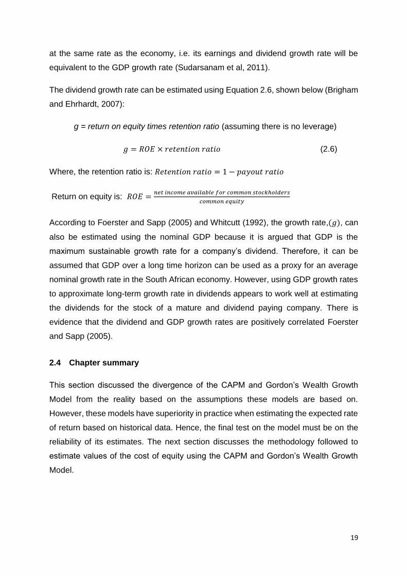
𝑔 = 𝑅𝑂𝐸 × 𝑟𝑒𝑡𝑒𝑛𝑡𝑖𝑜𝑛 𝑟𝑎𝑡𝑖𝑜 (2.6)

Where, the retention ratio is: 𝑅𝑒𝑡𝑒𝑛𝑡𝑖𝑜𝑛 𝑟𝑎𝑡𝑖𝑜 = 1 − 𝑝𝑎𝑦𝑜𝑢𝑡 𝑟𝑎𝑡𝑖𝑜

Return on equity is: 𝑅𝑂𝐸 =𝑛𝑒𝑡 𝑖𝑛𝑐𝑜𝑚𝑒 𝑎𝑣𝑎𝑖𝑙𝑎𝑏𝑙𝑒 𝑓𝑜𝑟 𝑐𝑜𝑚𝑚𝑜𝑛 𝑠𝑡𝑜𝑐𝑘ℎ𝑜𝑙𝑑𝑒𝑟𝑠

𝑐𝑜𝑚𝑚𝑜𝑛 𝑒𝑞𝑢𝑖𝑡𝑦

According to Foerster and Sapp (2005) and Whitcutt (1992), the growth rate,(𝑔), can

also be estimated using the nominal GDP because it is argued that GDP is the

maximum sustainable growth rate for a company’s dividend. Therefore, it can be

assumed that GDP over a long time horizon can be used as a proxy for an average

nominal growth rate in the South African economy. However, using GDP growth rates

to approximate long-term growth rate in dividends appears to work well at estimating

the dividends for the stock of a mature and dividend paying company. There is

evidence that the dividend and GDP growth rates are positively correlated Foerster

and Sapp (2005).

2.4 Chapter summary

This section discussed the divergence of the CAPM and Gordon’s Wealth Growth

Model from the reality based on the assumptions these models are based on.

However, these models have superiority in practice when estimating the expected rate

of return based on historical data. Hence, the final test on the model must be on the

reliability of its estimates. The next section discusses the methodology followed to

estimate values of the cost of equity using the CAPM and Gordon’s Wealth Growth

Model.

20

3 DATA AND METHODOLOGY

3.1 Introduction

This chapter provides a description of the data and methodology utilised in explaining

the differences in the cost of equity values for selected mining companies. The study

focuses on the CAPM and Gordon’s Wealth Growth Model for the reasons provided in

Chapter 2. Section 3.2 describes the sources of data and nature of the data required

for this research. The parameters used to estimate the rate of return are discussed in

Sections 3.3 to 3.4.

3.2 Data from JSE-listed mining companies

The research is limited to mining companies quoted on the Johannesburg Securities

Exchange (JSE). The JSE was selected because of the following reasons:

It is a member of the World Federation of Exchanges and one of the most

reliable trading platforms in the world;

It adheres to global standards and legislative requirements;

It acts as a regulator to its members and ensures that markets operate in a

transparent manner, ensuring investor protection;

It ensures accurate and sufficient disclosure of all information relevant to

investors (City of Johannesburg, 2014);

JSE data can be accessed for a sufficient length of time.

The sectors of the JSE were defined differently prior to June 1995, so one will have to

reconstruct each sectoral index in order to obtain data prior to June 1995.

Reconstruction of the data is beyond the scope of this study, thus, only data post 1995

was used. The JSE was illiquid prior to 1998; therefore, the time horizon period for the

study is January 1998 to December 2012. Data for the last five years was reserved for

the purpose of forecast valuation. Moreover, the top mining companies, by market

capitalisation, are used in this study as the smaller companies are thinly traded. Larger

mining companies are unlikely to experience extended periods of mispricing compared

to smaller companies, which will have dire effects on the findings if it occurs.

21

Gordon’s Wealth Growth Model is useful when valuing companies that regularly pay

dividends and have stable growth. Small mining enterprises do not pay dividends

frequently and have variations in growth rates, thus, it will be futile to determine their

discount rates using this model. Tholana et al (2013) stated that gold, platinum and

coal are the most important minerals in South Africa; hence, the focus of this study is

confined to these commodities. However, in this study only gold and platinum were

analysed because Gordon’s Wealth Growth Model can only be applied to companies

paying dividends. Therefore, coal-mining companies (not multi-commodity) were not

considered because they did not pay dividends regularly to be classified as ‘stable

growth’ companies. The top three (3) mining companies, by market capitalisation,

quoted on the JSE over the period of the study were selected for platinum and gold

mining companies. The mining companies used were:

Platinum: Anglo American Platinum Limited, Lonmin Plc and Impala Platinum

Holdings Limited;

Gold: AngloGold Ashanti Limited, Harmony Gold Mining Company Limited and

Gold Fields Limited;

Data for the purpose of this research was collected from I-Net Bridge, McGregor BFA

and Bloomberg databases. Table 3.1 provides a summary of the data gathered from

the above-mentioned sources. Returns, betas and standard deviations were

computed using Microsoft’s Excel spreadsheet program, see Appendix 7.1-7.7.

Table 3.1 Databases and data collected

Database

I-Net Bridge

McGregor BFA

Bloomberg

Data collected

Historical monthly closing prices of shares

Dividend payouts

South African government bond yields

Dividend yields

Actual beta values

WACC values split into debt and equity components (Bloomberg only)

22

The frequency of data is monthly similar to various studies as discussed in Section

2.2.2. The monthly return for a stock, 𝑖 is calculated using the formula in Equation 3.1.

𝑅𝑖 =(𝑆𝑖,𝑡−𝑆𝑖,𝑡−1)+ 𝐷𝑖,𝑡

𝑆𝑖,𝑡−1 (3.1)

Where:

𝑅𝑖 is the return for stock, 𝑖;

𝑆𝑖,𝑡 is the stock price at the present time;

𝑆𝑖,𝑡−1 represents the asset price at the previous month;

𝐷𝑖,𝑡 is the dividend price at the present time for the stock.

According to Marx et al (2009), the market portfolio contains all risky financial assets

(for instance debentures, options, shares, etc.) and risky real assets (i.e. jewellery,

precious metals, real estate, etc.). This kind of a market is not discernible, thus, a

broad-based share index is used as proxy for the market portfolio. Bradfield (2003)

agreed that there is no practical way to conduct a test with reference to the actual

market portfolio. Roll (1977) stated that unless the precise composition of the true

market is known, the probability of the proxy for the market portfolio being mean-

variance with the true market portfolio is directly unverifiable. Consequently, the

FTSE/JSE All Share Index was used as the proxy for the market portfolio.

WACC can be pre-tax or after-tax and these two are related by the following general

formula:

WACCpt = WACCat / (1-t) (3.2)

Where WACCat is the weighted average cost of capital after-tax; WACCpt is the

weighted average cost of capital pre-tax; and t is the corporate income tax rate. The

cost of debt in WACC is tax deductible hence the term (1-t) while cost of equity does

not have tax treatment and is therefore the same cost either pre- or post-tax. It is for

this reason that the cost of equity component of WACC was extracted and used as the

benchmark for testing the reliability of either CAPM or Gordon’s Wealth Growth Model

estimates. In other words the pre-tax CAPM estimates were compared independently

23

of the post-tax Gordon’s Wealth Growth Model estimates in order to determine which

model closely estimated the cost of equity.

3.3 CAPM research methodology

Beta is calculated as the slope coefficient of the OLS linear regression equation using

monthly return data over the period of the preceding 60 months against the All Share

Index (ALSI) on the X-axis. Coefficients of determination, which measure the degree

to which the estimated beta is explained by the previous beta coefficient, were

calculated for the same values as the ones utilised in the estimation of beta values.

Microsoft Excel’s r-squared (RSQ) function was used to calculate the coefficient of

determination. Correcting for regression bias was calculated using Blume’s technique

for all time periods for each mining company.

The holding period used in this report is inadequate to estimate reliable risk-free rate

and equity risk premium. Therefore, values used as proxies in various studies

determined over long time horizon were used. Fernandez et al (2013) provided

estimates of market risk premium and risk-free rate used for various countries. The

values used in South Africa have remained relatively stable from 2011 to 2013.

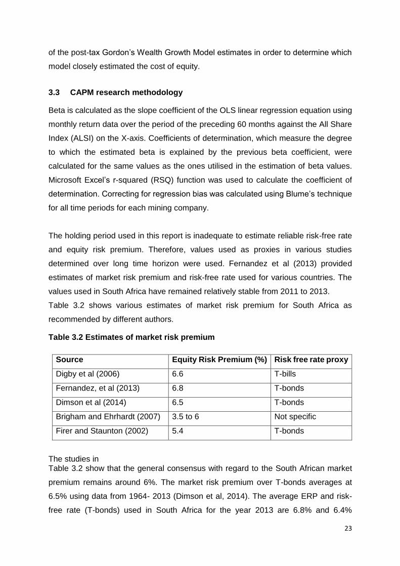
Table 3.2 shows various estimates of market risk premium for South Africa as

recommended by different authors.

Table 3.2 Estimates of market risk premium

Source Equity Risk Premium (%) Risk free rate proxy

Digby et al (2006) 6.6 T-bills

Fernandez, et al (2013) 6.8 T-bonds

Dimson et al (2014) 6.5 T-bonds

Brigham and Ehrhardt (2007) 3.5 to 6 Not specific

Firer and Staunton (2002) 5.4 T-bonds

The studies in Table 3.2 show that the general consensus with regard to the South African market

premium remains around 6%. The market risk premium over T-bonds averages at

6.5% using data from 1964- 2013 (Dimson et al, 2014). The average ERP and risk-

free rate (T-bonds) used in South Africa for the year 2013 are 6.8% and 6.4%

24

respectively (Fernandez et al, 2013). These estimates were adopted for this study in

order to reduce the error in the estimated cost of equity.

3.4 Gordon’s Wealth Growth Model research methodology

As discussed in Section 2.3 that it is vital to take a view of long-term that a company

will grow at the rate of the economy, therefore, GDP growth rate was adopted as a

proxy for company’s growth rate. GDP measures the level of economic activity for a

country. Changes in the GDP figure are negligible when measured from year to year

and can be predicted with acceptable accuracy. The constant growth rate proxy used

was the GDP rate over a relatively long period to reduce the effect of variations due to

market fluctuations. The GDP rate was based on the annualized percentage change

for seasonally adjusted quarterly gross domestic product (Fama and French, 1988;

Shepherd, 1987).

3.5 Descriptive statistics

Descriptive statistics are used to illustrate the major dataset features because they are

a rapid and brief way to extract the characteristics of the data. The descriptive statistics

included in the analysis of the data are the mean, standard deviation, range, sum, box

and whiskers plot and correlation coefficient. A summary of the descriptive statistics

for mining companies is shown in Appendix 7.8. The mean describes the central

tendency of the data. However, if there is an outlier, the arithmetic mean value does

not become the true representative of the central tendency of the data. An outlier has

the same impact on the standard deviation as it has on the mean. Therefore, the box

and whisker plot (box plot) was adopted to further analyse the data because it is based

on the robust statistics thus its resists the effect of outliers (Massart et al, 2005; Potter,

2006).

When using box and whisker plot the mean is replaced by a median that is the middle

observation in a ranked dataset. The interquartile range describes the spread of the

data that is the range where the middle 50% of data is found (Potter, 2006), see

Appendix 7.9. The correlation coefficient is one of the most utilised statistical method

in summarising research data (Taylor, 1990). This coefficient was used to examine the

http://liberta.co.za/blog/what-is-gross-domestic-product/

25

degree of the linear relationship between the CAPM and Gordon’s Wealth Growth

Model with the equity component of WACC.

3.6 Chapter summary

This chapter dealt with the data sources and data used in the study and the

methodology employed to calculate parameters necessary to estimate the rate of

return using the commonly applied CAPM and Gordon’s Wealth Growth Model. The

next section presents the results obtained from the analysis of the data.

26

4 RESULTS AND DISCUSSION

4.1 Introduction

This chapter presents the estimation results of the CAPM and Gordon’s Wealth

Growth Model. A model that explained better the differences in the cost of equity

values for the mining companies under review was recommended. The WACC values

obtained from the Bloomberg database were utilised as benchmark for analysis in

explaining the differences in the estimated cost of equity, see Appendix 7.10. In order

to have a meaningful comparison it was important to split the WACC into its debt and

equity components so that CAPM and Gordon’s Wealth Growth Model could be

benchmarked against the equity component of WACC.

The cost of equity estimates calculated using the CAPM model in this study were

derived using readily available pre-tax T-bond rates as the risk-free rate. The input

values for the CAPM equation are risk free rate and ERP of 6.4% and 6.8%,

respectively. The beta values were calculated using the OLS linear regression,

covariance of stock returns against the market returns and adjusted using the Blume’s

technique. The adjusted beta coefficient for the preceding 60 months was used to

estimate the cost of equity.

Gordon’s Wealth Growth Model assumes that dividends grow at a constant rate to

perpetuity. The cost of equity estimates calculated using the Gordon’s Wealth Growth

Model in this study were derived using post-tax dividends. Subsequently, the GDP rate

was applied as an alternative to company specific growth rates, which are not constant

over time. The GDP growth rate in South Africa averaged 3.16% in real terms from

1993 until 2014, as shown in Figure 4.1.

27

Figure 4.1 South African real GDP growth rate: 1993-2014

Source: Taborda (2014)

The real GDP rate was used to calculate the nominal GDP rate by applying the effect

of inflation. The ability to forecast the rate of inflation over a reasonable period

accurately is highly unlikely due to its volatility (Bora, 2013) (Barnett and Sorentino,

1994). According to Aisen and Veiga (2006), the main causes of inflation volatility are

political instability; lower economic freedom; political fragmentation and higher degree

of ideological polarization. Barnett and Sorentino (1994) alluded that a single inflation

rate based on recent values be used. Stowe et al (2007) and Sudarsanam et al (2011)

suggested that a long-run inflation rate be applied in estimating the cost of equity using

the Gordon’s Wealth Growth Model.

The inflation rate used in South Africa is usually the inflation based on the consumer

price index (CPI). The CPI shows the change in prices of standard households goods

and services purchased for consumption. The inflation rate in South Africa averaged

6.26% from 1993 until 2013 on year-on-year changes of the CPI (Statistics South

Africa, 2013).

Nominal GDP growth rate was calculated using Fisher’s effect (Bora, 2013) shown in

Equation 8:

(1 + 𝑅) = (1 + 𝑟) × (1 + 𝑖) (8)

28

Where:

𝑅 is the nominal GDP growth rate;

𝑟 is the real GDP growth rate;

𝑖 is the inflation rate.

There was no change in dividend pay-out ratios or dividend yield rates noted for the

companies during the period under study, which might have impacted to a lesser

degree, the reliability of the Gordon’s Wealth Growth Model.

4.2 The impact of the Global Financial Crisis on the South African mining

industry

The period over which the study is undertaken covers an era of commodities boom

and bust. The commodity boom commenced in 2001 driven by material-intensive

growth in developing countries and emerging economies such as China, Russia, India

and Brazil; weakening US dollar; reasonable growth in the advanced economies and

constraint in material supply from mining companies. These factors worked together

to drive the commodity price upwards between 2001 and mid-2008 as alluded to by

Padayachee (nd) and Baxter (nd).

In 2008, the global commodity market crashed slowing down economic growth, for

instance, the South African economic growth rate plummeted to 1.8% in the last

quarter of 2008, then dropped further to -3.2% in the second quarter of 2009. The

economic growth slowdown affected the world for minerals and companies had to

restrict supply in response to weakening demand environment as mentioned by

Padayachee (nd) and Baxter (nd). Njowa et al (2014) alluded that since the Global

Financial Crisis (GFC) of mid-2008, it has been difficult to obtain capital for mining

projects.

Estimating the cost of equity during market bull and bear periods may yield results

rendering the model applied unsuitable to estimate the discount rate. Therefore, it is

vital during the period of estimation to take into account all external factors that might

affect the results.

29

4.3 Cost of equity for platinum mining companies

The platinum mining industry was severely affected by the GFC causing a reduced

demand for the commodity. The price of platinum plunged from US$ 2048 per ounce

in May 2008 to US$ 834 per ounce by December 2008. Subsequently, the companies

adopted cost saving strategies in order to remain in business (Donovan, 2013). Figure

4.2 shows that dividends paid by all the platinum mines dropped post the recession,

with only Impala declaring dividends in 2009. Therefore, it is clear that the Global

Financial Crisis affected the platinum industry significantly.

In 2012 platinum miners were hit by low prices, wildcat industrial strikes across almost

all PGM producers, safety stoppages and inflationary pressures on costs. Anglo

American Platinum and Lonmin did not pay dividends citing future funding

commitments and uncertainty in global economic markets as the main reasons. Impala

Platinum declared dividends in FY2012 because the lower prices were offset by a

weaker Rand/Dollar exchange rate (Anglo American Platinum, 2012; Impala Platinum,

2012; Lonmin, 2012).

Figure 4.2 Declared dividends per share for platinum mining companies

30

4.3.1 Anglo American Platinum

The discount rate estimates for FY2002 to FY2012 period are shown in Figure 4.3.

The estimates are divided according to different phases according to event

occurrences. The phases are labelled as ‘A’, ‘B’ and ‘C’ representing the periods of

market boom; recession and steady economic growth, respectively. During Phase A

(boom period), the commodity prices increased drastically due to increased global

demand of platinum group metals (PGMs). Anglo American Platinum saw improved

headline earnings because of higher US dollar prices realised in metals sold and

weaker rand/US dollar exchange rates.

However, while demand was growing, South African producers failed to gain from such

price increases because they were experiencing operational challenges that reduced

their supply into the market. These challenges include industrial action; safety-related

production stoppages; shortage of skilled labour and processing bottlenecks. Failure

to meet the set production targets and supply demands may have a negative impact

on a company, which is evident in an increasing risk profile of a company. The effect

of these challenges can be seen in Figure 4.3 where values for the equity component

of WACC were on a steady increase during Phase A.

Figure 4.3 Cost of equity for Anglo American Platinum from FY2002 to FY2012

31

In Phase B (recession period), both the estimate cost of equity rates for CAPM are flat

and that for Gordon’s Wealth Growth Model show a sharp decrease while the actual

discount rate shows an upward trend. The Global Financial Crisis curbed the demand

of PGMs, causing a price decline. Anglo American Platinum suffered a decrease in

headline earnings per ordinary share of 95% in FY2009 due to lower US dollar prices

realised on metals sold.

In Phase C (steady economic growth period), in the second half of 2009, there were

signs of market recovery with a consequential increase in metal demand and

recovering prices. However, no dividends were paid in FY2009 sighting the need to

retain cash for maintenance of operations as the main reason. Anglo American

Platinum focused on cost management strategies (curtailing non-value adding

operations such as putting high cost shaft Siphumelele 3 on care and maintenance),

which had an effective contribution to the company’s performance (Anglo American

Platinum Limited, 2010). It can be seen from Figure 4.3 that both the CAPM and

Gordon’s Wealth Growth Model failed to estimate the actual discount rates during

periods of economic instability observed throughout the period under study.

4.3.1.1 Descriptive statistics for Anglo American Platinum

The descriptive statistics tool was adopted in order to be able to analyse the data from

equity component of WACC, CAPM and Gordon’s Wealth Growth Model. Descriptive

statistics allow data to be presented in a more meaningful manner from which, simpler

interpretation can be performed. The relationship between actual and estimated

discount rates was analysed checking how similar the values are to each other by

looking at the mean squared error (MSE), mean, standard deviation, range, sum,

correlation coefficient and box and whisker plot.

Estimated discount rates using CAPM and Gordon’s Wealth Growth Model are

contrasted against the equity component of WACC values in Table 4.1 using MSE.

The actual cost of equity for Anglo American Platinum in FY2010 was 23.78%, which

is higher than the other years. This may be attributed to the reaction to the GFC that

curbed the demand for the PGMs; lower US dollar prices on metals sold experienced

in 2009 (Anglo American Limited, 2009).

32

Table 4.1 Cost of equity and the mean squared error for Anglo American

Platinum

The mean square error between the equity component of WACC and either of the

models must be zero to prove that there is similarity between actual and estimated

cost of equity values. From Table 4.1, it can be seen that CAPM and Gordon’s Wealth

Growth Model produce similar estimates for the MSE that are very close to zero.

However, when considering the years individually, Gordon’s Wealth Growth Model

produces more values of MSE close to zero. The main problem with using unweighted

mean as measure of analysis is that all values are assumed to have the same

weighting. Therefore, when there is a wider range in values, as observed with

Gordon’s Wealth Growth Model, the calculated mean is biased towards narrowly

spread values (Massart et al, 2005). Hence, it is important that other measures are

employed in an analysis.

Statistical analysis using some of the measures is presented in Table 4.2 for the CAPM

and the Gordon’s Wealth Growth Model against the equity component of WACC.

Gordon’s Wealth Growth Model has a mean of 14%, which is close to that of the equity

component of WACC of 12% while CAPM has a mean of 16%.

33

Table 4.2 Descriptive statistics for Anglo American Platinum

Measure

Equity

component of

WACC

CAPM Gordon's Wealth

Growth Model

Mean 12.40% 16.10% 13.80%

Standard deviation 4.60% 1.10% 3.40%

Range 16.70% 4.10% 11.00%

Correlation coefficient 1.00 0.19 0.31

Sum 136.80% 176.80% 151.60%

The standard deviation for Gordon’s Wealth Growth Model is similar to that of the

equity component of WACC by approximately 74% while that of CAPM is about 24%.

Therefore, the spread of data around the average for the equity component of WACC

and Gordon’s Wealth Growth Model is almost identical. As with the analysis using

MSE, the range of Gordon’s Wealth Growth Model is close to that of the equity

component of WACC whereas CAPM differs by approximately 76%. The main cause

of this disparity is because the spreads of Gordon’s Wealth Growth Model and the

equity component of WACC values are wide while the estimates of CAPM have a

narrow spread.

The sum yields the same results as with the other measures, Gordon’s Wealth Growth

Model showing superiority over CAPM. The cost of equity estimates from Gordon’s

Wealth Growth Model vary from 9.62% to 17.25% while the CAPM estimates vary from

13.13% to 17.18%. Hence, the average discount rates are 13.78% and 16.07% for

Gordon’s Wealth Growth Model and CAPM, respectively, proving that CAPM has

higher estimates.

Correlation of the equity component of WACC rates with the cost of equity estimates

from CAPM and Gordon’s Wealth Growth Model was tested. Perfect correlation exists

if all values lie on a straight line and the correlation coefficient is at a unity. The

34

correlation coefficient values are very weak for both models (see Table 4.2); however,

Gordon’s Wealth Growth Model has a better correlation with the equity component of

WACC than CAPM. The spread for CAPM data distribution is narrower as illustrated

in Figure 4.4. The interquartile ranges (IQR) for the equity component of WACC and

Gordon’s Wealth Growth Model are 0.05 and 0.05, respectively. The IQR for CAPM is

0.01, which is significantly different from that of the equity component of WACC; this

is expected because the spread of the CAPM data is narrower, see Table 4.1.

Figure 4.4 Box and whisker plot for Anglo American Platinum cost of equity

4.3.1.2 Summary for Anglo American Platinum

The cost of equity estimates using the CAPM and Gordon’s Wealth Growth Model

failed to predict the actual discount rates for Anglo American Platinum. Descriptive

statistics were used to check for similarity in the data for CAPM and Gordon’s Wealth

Growth Model with the equity component of WACC rates. The statistics measures

show that the data for Gordon’s Wealth Growth Model and the equity component of

WACC are similar only MSE results favouring CAPM when looking at the means.

35

4.3.2 Impala Platinum Holdings Limited

The cost of equity rates were divided into phases according to the events occurring

during the period under study as labelled in Figure 4.5. In Phase A, the platinum group

metals (PGMs) prices surged because of the demand driven by emerging markets.

The high US dollar revenue realised from sales and weak rand against the US dollar

exchange rate resulted in improved earnings for Impala Platinum. The platinum

industry could not meet the demand from the markets thus metal prices increased

beyond expectations (Impala Platinum Holdings Limited, 2007). The increase in the

actual risk profile for the company may be alluded to safety related stoppages and

failure to meet set production output, as seen in Figure 4.5 where the equity

component of WACC rates were increasing from FY2004 to the beginning of Phase

B.

Figure 4.5 Cost of equity for Impala Platinum from FY2002 to FY2012

Phase B depicts a continuing increase in the actual discount rate while Gordon’s

Wealth Growth Model shows a sharp decrease in the risk profile of the company. The

estimated cost of equity for CAPM is relatively flat. The Global Financial Crisis affected

the mining industry as a whole and Impala Platinum was no exception. The cost of

equity for the company kept increasing because of a decline in earnings resulting from

low production output and high labour cost attributed to the disposal of Aquarius

36

Platinum assets and a 10% wage increase. In FY2009, the electricity cost increased

by 24%; labour cost by 14.6% and other metal prices fell and the company’s credit

rating was under review.

The period post-recession, Phase C, was a challenging period for Impala Platinum as

the company was faced with strike action at the beginning of 2010, soaring electricity

cost and a wage increase of 11%. All these factors contributed to the declining

headline earnings realised (Impala Platinum Holding Limited, 2010). In FY2012,

Impala Platinum had reduced headline earnings by 38% compared to FY2011 due to

industrial strike action and Section 54 stoppages resulting in low production levels

(Impala Platinum Holdings Limited, 2012).

Despite all these factors mentioned above, the equity component of WACC started to

drop post-recession, whereas the estimate discount rates for Gordon’s Wealth Growth

Model captured the pressure imposed by these factors. The estimate cost of equity for

CAPM had a slight increase.

4.3.2.1 Descriptive statistics for Impala Platinum

The actual cost of equity for Impala Platinum in 2010 was 21.97% an increase from

the previous year, which may be alluded to the response to the Global Financial Crisis,

increase in cash operating costs and strike action, see Table 4.3 (Impala Platinum

Holdings Limited, 2010).

Table 4.3 Cost of equity and the mean squared error for Impala Platinum

37

As the economic market stabilised post the recession period, the equity component of

WACC rates started to decline. The mean squared error for both CAPM and Gordon’s

Wealth Growth Model is 0.004, thus, this measure is not conclusive. Table 4.4 displays

the statistical analysis using mean, standard deviation, range and sum to contrast

CAPM and Gordon’s Wealth Growth Model against the equity component of WACC.

Table 4.4 Descriptive statistics for Impala Platinum

Measure

Equity

component

of WACC


Growth Model

Mean 14.00% 16.00% 14.20%


Range 14.40% 6.00% 6.50%


Sum 153.60% 176.20% 156.20%

The mean for Gordon’s Wealth Model is 14.20% and it is approximately equal to that

of the equity component of WACC while the mean for CAPM is 16.00% that is 2%

more. The standard deviation values for Gordon’s Wealth Growth Model and CAPM

are different from the one for the equity component of WACC. The spread of data

around averages for these models is not similar, with CAPM having a narrower spread.

The sum for the equity component of WACC and Gordon’s Wealth Growth Model are

relatively similar while that of CAPM is much higher. This disproportion may be

attributed to the high estimate cost of equity rates from CAPM.

The average discount rates for CAPM, Gordon’s Wealth Growth Model and the equity

component of WACC are 16.02%, 14.20% and 13.96%, respectively. Therefore, the

Gordon’s Wealth Growth Model has superiority over CAPM based on these measures

presented in Table 4.4. From Table 4.4, it can be seen that there is a modest

correlation between the equity component of WACC and CAPM. There is low

38

correlation between Gordon’s Wealth Growth Model and the equity component of

WACC.

Box and whisker plots provide a picture of continuous data, as shown in Figure 4.6.

The distribution of CAPM is much narrower when compared to the other two models.

The spread for CAPM rates is narrower as expected since the estimate values in Table

4.4 have a small range of 0.06.

Figure 4.6 Box and whisker plot for Impala Platinum cost of equity

4.3.2.2 Summary for Impala Platinum

The CAPM and Gordon’s Wealth Growth Models failed to estimate the discount rates

for Impala Platinum during the period under review. The similarity of the data set was

checked using descriptive statistics; however, there is no strong model preferred

based on the analysis.

4.3.3 Lonmin Plc

The cost of equity rates for CAPM, Gordon’s Wealth Growth Model and the equity

component of WACC are shown in Figure 4.7. In Phase A (from 2002 to mid-2008),

39

on average the equity component of WACC rates for Lonmin were on the increase

from FY2004 to FY2008. This discount rate increase may be attributed to a decrease

in company earnings due to a drop in production output, inflationary pressures in the

South African mining industry resulting in high production costs (Lonmin Plc, 2007).

Figure 4.7 Cost of equity for Lonmin from FY2002 to FY2012

In Phase B, All the models show that there is a decrease in the cost of equity values

even though it was during a recession period. When the price for PGM ounce

plummeted by 49% in FY2009 compared to FY2008, Lonmin adopted cost cutting

initiatives. The cost cutting initiatives included, inter alia, closure of unprofitable

operations (such as the open cast at Marikana); restriction on capital expenditure;

suspension of dividend payouts and shedding of 20% of the employees thus reducing

costs. The relocation of management from London to Johannesburg in order to

enhance day-to-day executive management close to operations might have positively

impacted on the company risk profile (Lonmin Plc, 2009).

In the second half of 2009, there was optimism that the market would have a steady

recovery supported by the recovery of the automotive and industrial sectors. In

FY2010, Lonmin suffered unexpected problems with the Number One Furnace

resulting in higher operational costs. The rand strengthened against the US dollar;

however, its effect was outweighed by high dollar PGMs prices realised throughout

40

the year. The company did not meet its production targets due to safety stoppages

and skill shortages (Lonmin Plc, 2010).

The benefits of an operational turnaround implemented in 2009 and 2010 were only

realised in FY2011. However, illegal industrial actions, safety stoppages were major

challenges faced by the company (Lonmin Plc, 2011). The discount rates started

falling from the FY2010 level, this may be attributed to successful implementation of

cost saving initiatives during the recession period.

Lonmin employees embarked on an illegal strike at Marikana, North West province in

South Africa that lasted for seven weeks. The issues around this illegal strike have

been subject to an ongoing judiciary inquiry at the time of writing this research report.

The company did not pay dividends because of the uncertainty in the global economic

markets (Lonmin Plc, 2012). The illegal strike action had a negative impact on the risk

profile of the company. Consequently, the cost of equity for Lonmin is expected to

increase. However, the actual discount rate in Phase C continued to drop in FY2012.

The financial impact of the Marikana strike is likely to be evident in FY2013 as seen in

FY2011 where the benefits of the cost saving initiatives implemented in FY2009 were

realised. The CAPM and Gordon’s Wealth Growth Model failed to estimate the actual

cost of equity.

4.3.3.1 Descriptive statistics for Lonmin

The effect of the Global Financial Crisis in 2008 and 2009 can be seen in FY 2010’s

discount rates, see Table 4.5. The cost of equity for the equity component of WACC

and CAPM were 19.93% and 16.33%, respectively. The discount rate for Gordon’s

Wealth Growth Model was 9.62% because the company did not pay dividends in

FY2009 thus affecting the calculation when using Gordon’s Wealth Growth Model.

41

Table 4.5 Cost of equity and the mean squared error for Lonmin

The mean squared error for CAPM is closer to zero at 0.002 than that of Gordon’s

Wealth Growth Model at 0.003. However, this measure cannot be used alone to

determine a model that best estimates the actual discount rates. The average cost of

equity estimates for the equity component of WACC, CAPM and Gordon’s Wealth

Growth Model are 11.78%; 15.54% and 12.98% respectively. The averages for the

equity component of WACC and Gordon’s Wealth Growth Model are closer to one

another than that of CAPM.

The mean for Gordon’s Wealth Growth Model is 13% is equal to the one for the equity

component of WACC whereas CAPM has a mean that is higher than the means from

the two models (Table 4.6). The standard deviation values for CAPM and Gordon’s

Wealth Growth Model are different from that of the equity component of WACC. This

may be attributed to the spread of data around the average.

42

Table 4.6 Descriptive statistics for Lonmin

Measure Equity

component of WACC


Growth Model

Mean 12.80% 15.50% 13.00%


Range 12.60% 3.70% 6.70%


Sum 141.30% 170.90% 142.80%

CAPM and Gordon’s Wealth Growth Model are identically correlated to the equity

component of WACC. The sum of values for the equity component of WACC and

Gordon’s Wealth Growth Model is approximately equal while that of CAPM is higher;

this is due to high estimate values for CAPM. The IQR values for the equity component

of WACC, CAPM and Gordon’s Wealth Growth Model are 0.060, 0.011 and 0.040

respectively (Figure 4.8). The spread for CAPM cost of equity estimates is narrower

and that is expected as the estimated values in Table 4.5 are closely spaced.

Figure 4.8 Box and whisker plot for Lonmin cost of equity

6%

8%

10%

12%

14%

16%

18%

20%

Equity component ofWACC

CAPM Gordon's WealthGrowth Model

Cost o

f e

qu

ity

Box plot for cost of equity

43

4.3.3.2 Summary for Lonmin

The CAPM and Gordon’s Wealth Growth Model failed to capture the cost of equity

rates during the period under study. During recession, CAPM managed to capture the

movement in discount rates but failed to estimate accurately the values as its

estimates were higher than that of the equity component of WACC rates. The average

discount rate for Gordon’s Wealth Growth Model approximates that of the equity

component of WACC but failed to capture the effect of recession on the cost of equity

for the company.

4.4 Cost of equity for gold mining companies

Gold is considered as a store of value and a safe haven during episodes of economic

insecurity. Investors have conventionally used gold as a hedge against inflation or a

falling currency. The price of gold experienced a secular increase in the years leading

to 2008 and 2009 in line with the commodity boom across the mining industry. When

the Global Financial Crisis deepened in the second half of 2008 with the collapse of

Lehman Brothers, the fears of global recession sent stock markets dipping in October

2008. However, the gold price soared up indicating a positive response to the financial

crisis. The increase in gold price was driven by the demand made up of jewellery,

industrial and investment demand (Baur and Lucey, 2009).

Figure 4.9 presents the dividend paid by gold mining companies during the period

leading to and post the Global Financial Crisis.

There was a reduction in the dividends declared by gold mining companies before

FY2006, with Harmony suspending dividends from FY2005 to FY2008, see Figure 4.9.

In FY2006, there was an increase in dividends payout by AngloGold Ashanti and Gold

Fields. The increase in dividends payout was attributed to the surge in demand for

physical gold from individuals in quest of wealth conservation instruments in the face

of geopolitical and economic uncertainty (AngloGold Ashanti Limited, 2006).

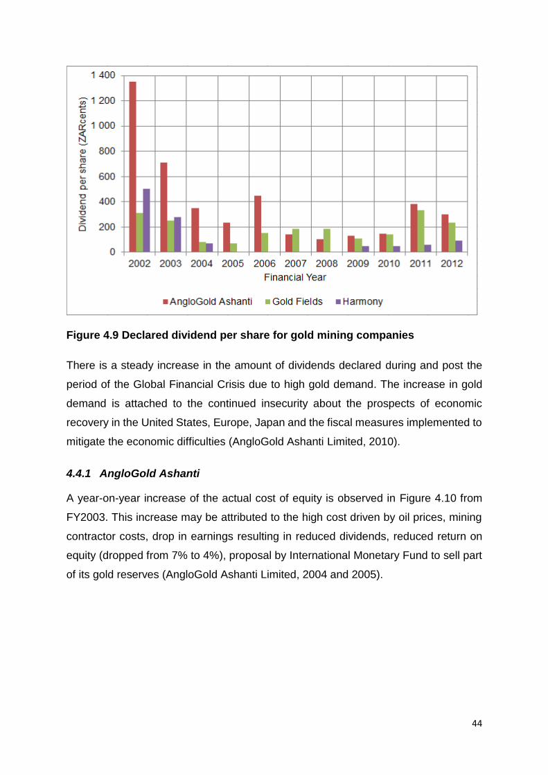
44

Figure 4.9 Declared dividend per share for gold mining companies

There is a steady increase in the amount of dividends declared during and post the

period of the Global Financial Crisis due to high gold demand. The increase in gold

demand is attached to the continued insecurity about the prospects of economic

recovery in the United States, Europe, Japan and the fiscal measures implemented to

mitigate the economic difficulties (AngloGold Ashanti Limited, 2010).

4.4.1 AngloGold Ashanti

A year-on-year increase of the actual cost of equity is observed in Figure 4.10 from

FY2003. This increase may be attributed to the high cost driven by oil prices, mining

contractor costs, drop in earnings resulting in reduced dividends, reduced return on

equity (dropped from 7% to 4%), proposal by International Monetary Fund to sell part

of its gold reserves (AngloGold Ashanti Limited, 2004 and 2005).

45

Figure 4.10 Cost of equity for AngloGold Ashanti from FY2002 to FY2012

The actual cost of equity for AngloGold Ashanti decreased in FY2006, this drop was

ascribed to investor and speculator interest combined with volatility in the first half of

the year that pushed the gold price to record highs. The Middle East and Chinese

jewellery fabrication and electronics industry increased the gold demand. The demand

for physical gold from individuals seeking wealth preservation instruments in the face

of economic market instability increased in FY2006 (AngloGold Ashanti Limited,

2006).

The cost of equity for AngloGold Ashanti surged up until the Global Financial Crisis

occurred due to various reasons. Some of the reasons are that higher gold price was

eroded by inflation, rehabilitation costs, lower-income from by-products, low

production output. The headline earnings of the company plunged by 32% (AngloGold

Ashanti Limited, 2007). During the Global Financial Crisis, Phase B, the discount rate

for AngloGold Ashanti decreased till the end of 2009 attributed to gold’s status as a

safe haven. When South Africa suffered a national power crisis, the mining industry

was adversely affected and forced to reduce the energy consumption to about 95%.

The rise in cost of equity between FY2009 and FY2010 may be attributed to the energy

issues related to insecurity of power supply and a proposed increase on the unit price

for energy (AngloGold Ashanti Limited, 2009).

46

The actual discount rates decreased from FY2010 to FY2012 due to the rise in gold

price. The rise in gold price was driven by the demand for gold as an investment

commodity during uncertainty about the prospect of economic recovery in the United

States, Japan and Europe. The demand for exchange traded funds (ETFs) grew by

7% in FY2011 as compared with FY2010. The credit rating of AngloGold Ashanti was

upgraded in March 2012 from Baa3 to Baa2 with stable outlook (AngloGold Ashanti

Limited, 2010; 2011 and 2012). The investment grade credit rating upgrade further

support the fall in discount rate seen in Figure 4.10. The CAPM and Gordon’s Wealth

Growth Model failed to estimates the actual cost of equity.

4.4.1.1 Descriptive statistics for AngloGold Ashanti

The mean squared error for CAPM is closer to zero than that of Gordon’s Wealth

Growth Model; however, they are not significantly different see Table 4.7. The estimate

cost of equity for CAPM are higher than the estimates for Gordon’s Wealth Growth

Model and that of actual discount rates.

Table 4.7 Cost of equity and the mean squared error for AngloGold Ashanti

A statistical analysis of data is presented in Table 4.8 and will be discussed in

conjunction with Figure 4.11. The range of the estimated discount rates for both

models is significantly different from that of the equity component of WACC values.

The estimate cost of equity had a narrower spread for CAPM and Gordon’s Wealth

Growth Model when compared to that of the equity component of WACC. This notion

47

was further supported by the range values of about 4% for CAPM and Gordon’s Wealth

Growth Model while the equity component of WACC had a range value of 9%.

Table 4.8 Descriptive statistics for AngloGold Ashanti

Measure Equity

component of WACC


Growth Model

Mean 10.40% 12.30% 11.40%


Range 8.80% 4.00% 4.40%


Sum 114.40% 135.60% 125.00%

Figure 4.11 Box and whisker plot for AngloGold Ashanti cost of equity

Figure 4.10 shows that there is an inverse relationship between Gordon’s Wealth

Growth Model and the equity component of WACC for 2002-2005 and 2011-2012

periods. Conversely, when analysing the whole period under study, there is a high

correlation between Gordon’s Wealth Growth Model and the equity component of

48

WACC while CAPM shows a very weak correlation with the equity component of

WACC (Table 4.8).

4.4.1.2 Summary for AngloGold Ashanti

Both CAPM and Gordon’s Wealth Growth Model were unable to provide reliable

estimates for the cost of equity. The cost of equity estimate for CAPM were decreasing

from 2007 and this is caused by beta values that were less than the market beta of

one, see Appendix 7.7. The beta values less than one indicate that AngloGold Ashanti

was less riskier than the market. The mean squared error values indicate that the

estimated cost of equity for both models are not significantly different from the actual

discount rates. The descriptive statistics show that there is similarity in data for the

equity component of WACC, CAPM and Gordon’s Wealth Growth Model. Gordon’s

Wealth Growth Model has very high correlation with the equity component of WACC

with a correlation coefficient of 0.9.

4.4.2 Gold Fields Limited

The actual cost of equity was on the rise from FY2003 with a slight decrease in FY2007

and continued to increase in FY2008 (Figure 4.12). Gold Fields was negatively

impacted by external issues like strengthening of rand against the US dollar, shortage

of skilled labour, power supply crisis and the national wage strike. The increase in gold

demand drove prices high and Gold Fields could have achieved high earnings. The

demand was due to continued political tensions in Iraq, North Korea and Middle East

and the rapid economic growth in China resulting in severe shortages of gold (Gold

Fields Limited, 2004; 2006; 2007 and 2008).

However, Gold Fields had other internal issues to address which hampered the gold

production output. Internal challenges faced by the company included amongst others,

the increase in cash costs due to wage increase above inflation rate, safety stoppages

due to fatalities and delay in construction; all affecting the amount of gold produced.

The investors were not satisfied with electricity supply security and safety performance

of the company leading to a volatile share price (Gold Fields Limited, 2004; 2006; 2007

and 2008).

49

Figure 4.12 Cost of equity for Gold Fields from FY2002 to FY2012

In Phase C, the actual cost of capital started to drop; this can be attributed to the cost

saving initiatives adopted by Gold Fields such as reduction of power consumption and

review of surface labour complement. The continued economic growth of emerging

markets like India and China underpinned strong demand for gold jewellery. Gold

Fields adopted a strategy of focusing only on cash generating operations by selling

high cost mines such as the selling of Beatrix and Kloof- Driefontein Complex (KDC)

mines to Sibanye Gold (Gold Fields Limited, 2012).

4.4.2.1 Descriptive statistics for Gold Fields

The mean squared error values for CAPM and Gordon’s Wealth Growth Model are at

0.003 in Table 4.9, which is almost equal to zero. The average cost of equity values

for the equity component of WACC, CAPM and Gordon’s Wealth Growth Model are

approximately similar. However, the effect of an outlier is evident in the average value

for the equity component of WACC because in FY2010 the cost of equity was 20.42%,

thus, introducing a bias into the average value.

50

Table 4.9 Cost of equity and the mean squared error for Gold Fields

The mean values for estimates of the equity component of WACC, CAPM and

Gordon’s Wealth Growth Model are equal, see Table 4.10. The range of values for the

equity component of WACC and Gordon’s Wealth Growth Model are similar whereas

CAPM is different, this is evident in Table 4.9. The correlation coefficient values states

that there is a moderate and weak correlation for Gordon’s Wealth Growth Model and

CAPM with the equity component of WACC, respectively. The sum of the values is

approximately similar, with Gordon’s Wealth Growth Model having minor superiority.

Table 4.10 Descriptive statistics for Gold Fields

Measure Equity

component of WACC


Growth Model

Mean 11.60% 11.70% 10.60%


Range 15.90% 6.50% 13.50%


Sum 127.40% 128.40% 116.80%

The spread of values can be seen in Figure 4.13, with Gordon’s Wealth Growth Model

having a narrower spread compared to CAPM values.

51

Figure 4.13 Box and whisker plot for Gold Fields cost of equity

4.4.2.2 Summary for Gold Fields

The CAPM managed to capture the trend in the post-recession phase, however, it

consistently underestimated the cost of equity. The Gordon’s Wealth Growth Model

failed to estimate an upward movement in the cost of equity. The descriptive analysis

was used to check the similarity of the data set for CAPM and Gordon’s Wealth Growth

Model with the equity component of WACC rates. The statistics measures show that

the data for Gordon’s Wealth Growth Model are similar to that of the equity component

of WACC with sum, mean, MSE providing inconclusive comparisons.

4.4.3 Harmony Gold Mining Company Limited

In Phase A, the CAPM managed to capture the trend of the actual cost of equity;

however, the discount rates for CAPM are overestimated, Figure 4.14. Harmony did

not declare dividends from FY2005 to FY2008; resulting in the estimate cost of equity

for this period using Gordon’s Wealth Growth Model being constant at 9.62%, see

Table 4.11. The main reason for not declaring dividends was cited to be the negative

impact on the business performance due to various reasons. The leading causes of

52

the poor performance were the exposure to the cyclical nature of the gold price over

preceding years and the volatility of the rand against the US dollar exchange rate, and

the company decided to use its earnings to fund growth projects. Harmony sold non-

strategic listed assets, such as Orkney shaft, and focused on turning loss-making

shafts into profit making operations (Harmony Gold Mining Company Limited, 2004;

2005; and 2007).

The performance of Harmony was further affected by the shortage of electricity supply

in 2008 resulting in closure of shafts and mining areas with high electricity

consumption. Consequently, the production targets were not met and thus affecting

the earnings. The Global Financial Crisis contracted equity funding, however,

Harmony managed to clear its debts during Phase B (Harmony Gold Mining Company

Limited, 2008 and 2009).

During Phase C, the discount rate for Harmony started declining and that can

attributed to the cost saving initiatives the company adopted, such as closure of the

HAR2, Evander 2, 5, and 7 shafts. The company resumed dividend payouts in FY2009

because the company was in a good financial position. The continued demand for gold

from India and China coupled with low production output kept the price of gold on a

steady increase (Harmony Gold Mining Company Limited, 2010; 2011 and 2012).

Figure 4.14 Cost of equity for Harmony from FY2002 to FY2012

53

4.4.3.1 Descriptive statistics for Harmony

The mean squared error values for CAPM and Gordon’s Wealth Growth Model are not

significantly different from zero, see Table 4.11. Therefore, the MSE is not a conclusive

measure and other measures were used from the descriptive statistics in Table 4.12.

The mean, standard deviation and range values for CAPM are similar to those of the

equity component of WACC attributed to the similarity in the spread of cost of equity

in Table 4.11.

Table 4.11 Cost of equity and the mean squared error for Harmony

Table 4.12 Descriptive statistics for Harmony

Measure Equity

component of WACC


Growth Model

Mean 11.70% 13.50% 11.00%


Range 12.90% 10.30% 5.90%


Sum 129.00% 148.80% 120.70%

CAPM has a better correlation with the equity component of WACC for 2004-2008

period which is a period before the GFC. In contrary, for the whole period, the Gordon’s

Wealth Growth Model has a high correlation with the equity component of WACC of

54

0.8 compared to a very weak correlation for CAPM. The sum of the Gordon’s Wealth

Growth Model was similar to that of the equity component of WACC, while CAPM has

a higher sum. It was expected for CAPM to have a high sum because of the high

estimated cost of equity, see Figure 4.14.

The box and whisker plot for Harmony is shown in Figure 4.15. The Gordon’s Wealth

Growth Model has a narrower spread than CAPM and the equity component of WACC.

This narrower spread is attributed to the period where there were no dividend paid,

see Figure 4.9.

Figure 4.15 Box and whisker plot for Harmony cost of equity

4.4.3.2 Summary for Harmony

The estimate cost of equity using Gordon’s Wealth Growth Model is not affected by

the reduction in dividends payout of the company but a cut in dividends payout causes

market value of the company to fall. Harmony did not declare dividends for a certain

period of time, which affected the ability of Gordon’s Wealth Growth Model to estimate

the cost of equity. The estimate cost of equity for CAPM started declining from FY2007

and underestimating the actual discount rates. The CAPM and Gordon’s Wealth

Growth Models failed to estimate the actual cost of equity values throughout the

55

period. However, Gordon’s Wealth Growth Model has a high correlation with the equity

component of WACC compared to a very low correlation for CAPM.

4.5 Chapter summary

This chapter presented the results and analysis for each company under study. The

discount rates were varying based on the state of the global economic market

performance, with low discount rates experienced during bullish periods. Both models

failed to estimate accurately the cost of equity for the companies under review. The

trend for cost of equity estimated using Gordon’s Wealth Growth Model is similar in all

platinum companies and the same applies for all gold companies considered in the

study. The CAPM has different trends for different companies, which can be attributed

to company’s individual risk profiles.

When the demand for PGMs from emerging markets increased, the price for PGMs

surged up resulting in high returns for PGMs producers, evident from the dividends

declared by companies. The Global Financial Crisis sent the demand of PGMs

plummeting, consequently, the price of PGMs dropped. There was a sharp rise in cost

of equity for platinum mining companies observed during Phase B. The discount rates

started dropping in Phase C, which may be attributed to the cost saving initiatives

companies adopted and a slow market recovery.

Investors redirected their investments from other commodity classes to gold when the

stock market collapsed in 2008. The gold price increased as the demand from

developed countries soared up for gold as an investment alternative. The cost of equity

for all gold mining companies was increasing sharply during Phase A. When the Global

Financial Crisis occurred, the rise in discount rates was relatively slow. The occurrence

of the Global Financial Crisis caused a high demand for gold as a safe haven and

investment instrument. Consequently, there was a drastic decrease in the cost of

equity for gold mining companies.

The correlation coefficient was used to summarise the findings of this study. Table

4.13 provides the rating system used to analyse the ability of CAPM and Gordon’s

Wealth Growth Model to estimate the cost of equity for mining companies.

56

Table 4.13 Rating system for asset pricing models

Coefficient of correlation

0 - 0.4 0.4 - 0.6 0.6 - 1.0

Rating poor moderate good

Colour red yellow green

Rating value 1 2 3

The colour classifications in Table 4.13 were assigned values in order to calculate an

overall rating score for CAPM and Gordon’s Wealth Growth Model. A summary of the

findings of this study using the correlation coefficient are shown in Table 4.14.

Table 4.14 Summary of findings based on correlation coefficient

The Gordon’s Wealth Growth Model has a higher overall rating compared to CAPM.

Hence, Gordon’s Wealth Growth Model was chosen as the better model to estimate

the cost of equity for mining companies. The next chapter will conclude the findings of

the research and provide recommendations.

57

5 CONCLUSIONS AND RECOMMENDATIONS

5.1 Introduction

This chapter recapitulates the findings, provide conclusions of the study and proposes

a way forward. Section 5.2 presents the summary with reference to the research

objectives. Limitations of the research and suggestions for future work are presented

in Section 5.3 and Section 5.4, respectively.

5.2 Findings and recommendations

Investment capital is a scarce resource of which mining companies compete for with

other industries. Therefore, it is vital that a present value for the project is determined.

A commonly used valuation technique is DCF analysis method to discount future cash

flows to present value using discount rates. There are various methods to determine

discount rates but this research considered Gordon’s Wealth Growth Model and

CAPM because of their simplicity and availability of the parameters required to

estimate the discount rates.

CAPM is the most commonly used method of estimating cost of equity for publicly

traded stocks as practitioners find its risk and return relation to be intuitive. This

method has strong theoretical backing; unfortunately, various authors have shown that

there is weak empirical evidence to support its use because it fails to capture various

anomalies. Some of the anomalies were discussed in Section 2.2.

Gordon’s Wealth Growth Model is regarded as the simplest form of dividend discount

models. This model is used to value stock of a firm that has stable growth and pays

out dividends. This model assumes that the stock is equal to the present value of all

its future dividend payments and dividends grow at a constant rate to infinite. The

drawback for this model is that there is no evidence in dividends for constant growth

to perpetuity, as depicted in Figure 4.2 and Figure 4.9 where some companies did not

pay dividends. Some of the anomalies experienced with Gordon’s Wealth Growth

Model were outlined in Section 2.2. Henceforth, the objective of this research was to

explain the differences in cost of equity estimated using CAPM and Gordon’s Wealth

Growth Model.

58

CAPM failed to capture the actual cost of equity throughout the period under study.

The estimate cost of equity were greater than the actual equity component of WACC

values in most cases. Gordon’s Wealth Growth Model captured the trend for actual

equity component of WACC values however, constantly underestimating the cost of

equity. This can be attributed to the fact that economic market movements do not

immediately affect the mining companies. The dataset for Gordon’s Wealth Growth

Model were similar to that of the equity component of WACC for both gold and platinum

mining companies. There was a high correlation between Gordon’s Wealth Growth

Model and the equity component of WACC for gold mining companies, whereas, a

weak correlation between the equity component of WACC and both CAPM and

Gordon’s Wealth Growth Model was identified for platinum mining companies.

However, CAPM had a narrower spread than Gordon’s Wealth Growth Model

throughout suggesting that it is a better model for estimating cost of equity.

The use of CAPM and Gordon’s Wealth Growth Model when the commodity market is

bullish or bearish rendered the models unsuitable to estimate the cost of equity for

mining companies. It is of paramount importance that external factors that affect the

results are taken into consideration. It is almost impossible to ascertain the weight

each external factor has on the result computed. From the findings in this report, it is

recommended that investors, practitioners and/or researchers consider using

Gordon’s Wealth Growth Model when estimating cost of equity for mining companies

under uncertain economic market conditions given that this method uses ex-ante data

to estimate ex-ante returns. This recommendation is however limited by the length of

the period under review and associated events within the review period. A longer time

horizon and larger sample-pool may lead to a different conclusion and

recommendation.

5.3 Limitations of the research

The limitations of this research are that:

The study is limited to two commodities with only the top three companies by

market capitalisation considered which may not be a true representative of the

mining industry;

59

The sample period of the research is fifteen (15) years, which is a short period

compared to studies done in the past. A short period may be subject to

increased standard errors in the data collected;

The research period includes phases of global market instability that may result

to inconsistencies in the data.

5.4 Recommendations for future work

The period of the research includes stages of global economic market uncertainty that

affected the results. Therefore, a similar study can be undertaken under stable global

economic conditions. This research only considered platinum and gold sectors, a

study for the South African mining industry can be carried out to explain differences in

cost of equity for various commodity classes. This study focused on estimating cost of

equity for mining companies, therefore, one can embark on a research to determine a

method that reliably estimate project specific discount rate. The cash flows upon which

the DCFs are based maybe in real or nominal money terms. An area for further

research is to determine whether the discounted cash flows should be in real or

nominal monetary terms.

60

6 REFERENCES

Aisen, A. and Veiga, F.J. (2006) Political instability and inflation volatility, International

Monetary Fund, working paper 06/212. INTERNET.

https://books.google.co.za/books?id=nqIGggwayGUC&pg=PA3&lpg=PA3&dq=cause

s+of+inflation+volatility&source=bl&ots=Vi49DEcgrI&sig=CYRWyI3wxmmBDXijGvof

6OvaRU0&hl=en&sa=X&ei=worTVKvBHsmBU_y7gcAK&ved=0CEgQ6AEwBg#v=on

epage&q=causes%20of%20inflation%20volatility&f=false. [Accessed 29 January

2015]

Anglo American Platinum Limited (2009) Annual report 2009. INTERNET.

http://www.angloamericanplatinum.com/~/media/Files/A/Anglo-American-

Platinum/annual-reports/ar2009.pdf, [Accessed 11 June 2014]


http://investoreports.com/angloplatinumar2010_pdfs//downloads/angloplatinum_201

0.pdf, Accessed on [11 June 2014]


http://www.angloamericanplatinum.com/~/media/Files/A/Anglo-American-

Platinum/annual-reports/aap-ar-2012-180213.pdf, [Accessed 11 June 2014]

AngloGold Ashanti Limited (2004) Annual report 2004. INTERNET.

http://www.anglogoldashanti.com/en/Media/Reports/Annual%20Reports/annual_fina

ncial_statements_report_2004.pdf, [Accessed 11 June 2014]

AngloGold Ashanti Limited (2005) Annual report 2005. INTERNET.

http://www.anglogoldashanti.com/en/Media/Reports/Annual%20Reports/annual-

financial-statements_report_2005.pdf, [Accessed 11 June 2014]

AngloGold Ashanti Limited (2006) Annual financial statements 2006. INTERNET.

http://www.anglogoldashanti.com/en/Media/Reports/Annual%20Reports/annual-

financial-statements-report_2006.pdf, [Accessed 11 June 2014]

https://books.google.co.za/books?id=nqIGggwayGUC&pg=PA3&lpg=PA3&dq=causes+of+inflation+volatility&source=bl&ots=Vi49DEcgrI&sig=CYRWyI3wxmmBDXijGvof6OvaRU0&hl=en&sa=X&ei=worTVKvBHsmBU_y7gcAK&ved=0CEgQ6AEwBg#v=onepage&q=causes%20of%20inflation%20volatility&f=false




http://www.angloamericanplatinum.com/~/media/Files/A/Anglo-American-Platinum/annual-reports/ar2009.pdf

http://www.angloamericanplatinum.com/~/media/Files/A/Anglo-American-Platinum/annual-reports/ar2009.pdf

http://investoreports.com/angloplatinumar2010_pdfs/downloads/angloplatinum_2010.pdf

http://investoreports.com/angloplatinumar2010_pdfs/downloads/angloplatinum_2010.pdf

http://www.angloamericanplatinum.com/~/media/Files/A/Anglo-American-Platinum/annual-reports/aap-ar-2012-180213.pdf

http://www.angloamericanplatinum.com/~/media/Files/A/Anglo-American-Platinum/annual-reports/aap-ar-2012-180213.pdf

http://www.anglogoldashanti.com/en/Media/Reports/Annual%20Reports/annual_financial_statements_report_2004.pdf

http://www.anglogoldashanti.com/en/Media/Reports/Annual%20Reports/annual_financial_statements_report_2004.pdf

http://www.anglogoldashanti.com/en/Media/Reports/Annual%20Reports/annual-financial-statements_report_2005.pdf

http://www.anglogoldashanti.com/en/Media/Reports/Annual%20Reports/annual-financial-statements_report_2005.pdf

http://www.anglogoldashanti.com/en/Media/Reports/Annual%20Reports/annual-financial-statements-report_2006.pdf

http://www.anglogoldashanti.com/en/Media/Reports/Annual%20Reports/annual-financial-statements-report_2006.pdf

61


http://www.anglogoldashanti.com/en/Media/Reports/Annual%20Reports/AGA_annua

l-financial-statements_2007.pdf, [Accessed 11 June 2014]


http://www.anglogoldashanti.com/en/Media/Reports/Annual%20Reports/AGA-

annual-financial-statements-2009.pdf, [Accessed 11 June 2014]

AngloGold Ashanti Limited (2010) Annual review. INTERNET.

http://www.anglogoldashanti.com/en/Media/Reports/Annual%20Reports/AGA-

annual-review-2010.pdf, [Accessed 11 June 2014]

AngloGold Ashanti Limited (2011) Annual integrated report 2011. INTERNET.

http://www.google.co.za/url?sa=t&rct=j&q=&esrc=s&frm=1&source=web&cd=1&ved=

0CBwQFjAA&url=http%3A%2F%2Fwww.aga-

reports.com%2F11%2Fdownload%2FAGA-annual-integrated-report-

2011.pdf&ei=dbHqVOCtBsS6Ub2ygbAK&usg=AFQjCNGCqxUFzg0QyW3I7Z_Dwnf

aC1i-dQ&sig2=gXx-FUKfQ8u8L9nSTw3SRw, [Accessed 11 June 2014]

AngloGold Ashanti Limited (2012) Annual integrated report 2012. INTERNET.

http://www.google.co.za/url?sa=t&rct=j&q=&esrc=s&frm=1&source=web&cd=1&sqi=

2&ved=0CBwQFjAA&url=http%3A%2F%2Fwww.aga-

reports.com%2F12%2Fdownload%2FAGA-annual-integrated-report-

2012.pdf&ei=ELHqVL_IFoHcUpWOg9gG&usg=AFQjCNEb8mVxYEONtOY4CEwZz

BxTzMgEkQ&sig2=Ui3Pr78d7t9tFkmIqmMMIA&bvm=bv.86475890,d.d24, [Accessed

11 June 2014]

Ballard, J. (1994) A practitioner’s view of DCF methods in mineral valuation,

Proceedings of Mineral Valuation Methodologies Conference, Sydney. INTERNET.

http://www.1mine.org/view/?d=1234567890123456789012345678901234567890123

456789012345678901234191782, [Accessed 13 February 2014]

http://www.anglogoldashanti.com/en/Media/Reports/Annual%20Reports/AGA_annual-financial-statements_2007.pdf

http://www.anglogoldashanti.com/en/Media/Reports/Annual%20Reports/AGA_annual-financial-statements_2007.pdf

http://www.anglogoldashanti.com/en/Media/Reports/Annual%20Reports/AGA-annual-financial-statements-2009.pdf

http://www.anglogoldashanti.com/en/Media/Reports/Annual%20Reports/AGA-annual-financial-statements-2009.pdf

http://www.anglogoldashanti.com/en/Media/Reports/Annual%20Reports/AGA-annual-review-2010.pdf

http://www.anglogoldashanti.com/en/Media/Reports/Annual%20Reports/AGA-annual-review-2010.pdf

http://www.google.co.za/url?sa=t&rct=j&q=&esrc=s&frm=1&source=web&cd=1&ved=0CBwQFjAA&url=http%3A%2F%2Fwww.aga-reports.com%2F11%2Fdownload%2FAGA-annual-integrated-report-2011.pdf&ei=dbHqVOCtBsS6Ub2ygbAK&usg=AFQjCNGCqxUFzg0QyW3I7Z_DwnfaC1i-dQ&sig2=gXx-FUKfQ8u8L9nSTw3SRw





http://www.google.co.za/url?sa=t&rct=j&q=&esrc=s&frm=1&source=web&cd=1&sqi=2&ved=0CBwQFjAA&url=http%3A%2F%2Fwww.aga-reports.com%2F12%2Fdownload%2FAGA-annual-integrated-report-2012.pdf&ei=ELHqVL_IFoHcUpWOg9gG&usg=AFQjCNEb8mVxYEONtOY4CEwZzBxTzMgEkQ&sig2=Ui3Pr78d7t9tFkmIqmMMIA&bvm=bv.86475890,d.d24







62

Barnett, D.W. and Sorentino, C. (1994) Discounted cash flow methods and the

Capital Asset Pricing Model, Mineral Valuation Methodologies Conference, Sydney,

pp. 17-35. INTERNET.

http://www.onemine.org/view/?d=12345678901234567890123456789012345678901

23456789012345678901234191789, [Accessed 18 July 2014]

Baur, D.G. and Lucey, B.M. (2009) Is gold a hedge or a safe haven? An analysis of

stocks, bonds and gold, School of Business and Institute for International Integration

Studies, The Financial Review 45, pp.217–229. INTERNET.

https://brianmlucey.files.wordpress.com/2011/05/gold_safehavenorhedge_fr.pdf,

[Accessed 12 January 2015]

Baxter, R. (undated) The global economic crisis and its impact on South Africa and

the country’s mining industry. INTERNET.

http://www2.resbank.co.za/internet/Publication.nsf/LADV/21EFDE8DEE8293534225

7601003680B6/$File/Roger%20Baxter.pdf. [Accessed 23 October 2014]

Benning, I. (2000) Bankers’ perspective of mining project finance, The Journal of The

Southern African Institute of Mining and Metallurgy, vol. 100, no. 3, May/Jun., pp.145-

152. INTERNET. http://www.saimm.co.za/Journal/v100n03p145.pdf, [Accessed 13

February 2014]

Blume, M.E. (1971) On the assessment of risk, The Journal of Finance, vol. 26, no.

1, Mar., pp. 1-10. INTERNET.

http://portaldace.mineco.gob.gt/sites/default/files/unidades/DefensaComercial/Casos

/Controversias/Inversionista%20-%20Estado/Etapa%20de%20Meritos%2007-

23%20(Ferrovias)/Respondent%20Experts/Spiller%20Exp%20Rpt%201st/LECG-38-

%20Blume%20(1971).pdf, [Accessed 06 May 2014]

Bodie, Z.V.I., Kane, A. and Marcus, A.J. (2002) INVESTMENTS, The McGraw-Hill

Companies, Inc. 1221 Avenue of the Americas, New York, USA.

Bora, B. (2013) Inflation effect on capital budgeting decisions, an analytical study,

International Journal of Conceptions on Management and Social Sciences, vol. 1,

no. 2, Dec. 2013. INTERNET.

http://www.worldairco.org/IJCMSS/December2013Paper154Spl.pdf. [Accessed 15

December 2014]



https://brianmlucey.files.wordpress.com/2011/05/gold_safehavenorhedge_fr.pdf

http://www2.resbank.co.za/internet/Publication.nsf/LADV/21EFDE8DEE82935342257601003680B6/$File/Roger%20Baxter.pdf

http://www2.resbank.co.za/internet/Publication.nsf/LADV/21EFDE8DEE82935342257601003680B6/$File/Roger%20Baxter.pdf

http://www.saimm.co.za/Journal/v100n03p145.pdf

http://portaldace.mineco.gob.gt/sites/default/files/unidades/DefensaComercial/Casos/Controversias/Inversionista%20-%20Estado/Etapa%20de%20Meritos%2007-23%20(Ferrovias)/Respondent%20Experts/Spiller%20Exp%20Rpt%201st/LECG-38-%20Blume%20(1971).pdf




http://www.worldairco.org/IJCMSS/December2013Paper154Spl.pdf

63

Bradfield, D. (2003) Investment basics XLVI, on the estimating the beta coefficient,

Investment Analysts Journal, no. 57, pp. 47-53. INTERNET.

http://pages.nes.ru/agoriaev/papers/bradfield%20on%20estimating%20the%20beta

%20coefficient%20iaj03.pdf, [Accessed 13 June 2014]

Bradfield, D., and Munro, B. (2011) Financial risk service on the Johannesburg Stock

Exchange, fourth quarter 2011, vol.22 no. 4. INTERNET.

http://www.lib.sun.ac.za/library/eng/finding/FRS/Cadiz%20FRS%20Betas%20Dec11.

pdf , [Accessed 12 May 2014]

Brigham, E.F. and Ehrhardt, M.C. (2007) FINANCIAL MANAGEMENT, Thomson

Learning, High Holborn House; 50-51 Bedford Row, London, Britain.

City of Johannesburg. (2014) Johannesburg Securities Exchange. INTERNET.

http://www.joburg.org.za/index.php?option=com_content&view=article&id=106%3Ajs

e&catid=30&Itemid=58 [Accessed 17 April 2014]

Damodaran, A. (2002) INVESTMENT VALUATION, Tools and Techniques for

Determining the Value of Any Asset, John Wiley & Sons, Inc., New York, USA.

Damodaran, A. (2008) What is the risk free rate? A search for the basic building

block, Stern School of Business. INTERNET.

http://people.stern.nyu.edu/adamodar/pdfiles/papers/riskfreerate.pdf, [Accessed

21June 2014]

Damodaran, A. (2012) Equity risk premium (ERP): determinants, estimation and

implications. INTERNET.

http://papers.ssrn.com/sol3/papers.cfm?abstract_id=2027211&download=yes,

[Accessed 21 June 2014]

Diacogiannis, G.P. (undated) Forecasting stock betas: evidence for the London

Stock Exchange, Warwick Business School. INTERNET.

http://digilib.lib.unipi.gr/spoudai/bitstream/spoudai/409/1/t39_n1-4_92to108.pdf,

[Accessed 26 November 2013]

http://pages.nes.ru/agoriaev/papers/bradfield%20on%20estimating%20the%20beta%20coefficient%20iaj03.pdf

http://pages.nes.ru/agoriaev/papers/bradfield%20on%20estimating%20the%20beta%20coefficient%20iaj03.pdf

http://www.lib.sun.ac.za/library/eng/finding/FRS/Cadiz%20FRS%20Betas%20Dec11.pdf

http://www.lib.sun.ac.za/library/eng/finding/FRS/Cadiz%20FRS%20Betas%20Dec11.pdf

http://www.joburg.org.za/index.php?option=com_content&view=article&id=106%3Ajse&catid=30&Itemid=58

http://www.joburg.org.za/index.php?option=com_content&view=article&id=106%3Ajse&catid=30&Itemid=58

http://people.stern.nyu.edu/adamodar/pdfiles/papers/riskfreerate.pdf

http://papers.ssrn.com/sol3/papers.cfm?abstract_id=2027211&download=yes

http://digilib.lib.unipi.gr/spoudai/bitstream/spoudai/409/1/t39_n1-4_92to108.pdf

64

Digby, P., Firer, C. and Gilbert, E. (2006) The South African equity risk premium,

Journal of Studies in Economics and Econometrics, vol. 30, no. 3, pp. 1-17.

INTERNET.http://reference.sabinet.co.za/webx/access/electronic_journals/bersee/be

rsee_v30_n3_a1.pdf, [Accessed 13 June 2014]

Dimson, E., Marsh, P., Staunton, M. and Mauboussin, M. (2014) CREDIT SUISSE

GLOBAL INVESTMENT RETURNS YEARBOOK 2014, Credit Suisse AG.

INTERNET.http://gallery.mailchimp.com/6750faf5c6091bc898da154ff/files/global_inv

estment_returns_yearbook_2014.pdf, [Accessed 07 August 2014]

Donovan, D.R. (2013) Prospecting for solutions: the challenges of South Africa’s

mining industry. INTERNET.

http://www.consultancyafrica.com/index.php?option=com_content&view=article&id=1

291:prospecting-for-solutions-the-challenges-of-south-africas-mining-

industry&catid=57:africa-watch-discussion-papers&Itemid=263, [Accessed 15

January 2014]

Ellis, T.R. (1995) Valuation methodologies for mines and mineral tenements, American

Institute of Minerals Appraisers, vol. 1, no. 5, Dec. pp. 1-7. INTERNET.

http://www.minevaluation.com/wp-

content/uploads/2012/09/EllisVal94ConfAIMA1295.pdf [Accessed 08 April 2014]

Ellis, T.R. and Collins, D.L. (2013) Discount rate selection methods applied in

appraisals of a quarry taken by eminent domain. INTERNET.

http://www.minevaluation.com/wp-

content/uploads/2013/04/CollinsEllis_DiscountRateCaseStudy_SME2013.ppt.pdf

[Accessed 07 April 2014]

Elton, E.J. and Gruber, M.J. (1995) MODERN PORTFOLIO THEORY AND

INVESTMENT ANALYSIS, John Wiley & Sons, Inc., New York, USA.

Fama, E.F. and French, K.R. (1988) Dividend yields and expected stock returns,

Journal of Financial Economics, vol. 22 no. 1, Oct., pp. 3-25 .INTERNET. boustred,


http://reference.sabinet.co.za/webx/access/electronic_journals/bersee/bersee_v30_n3_a1.pdf


http://gallery.mailchimp.com/6750faf5c6091bc898da154ff/files/global_investment_returns_yearbook_2014.pdf

http://gallery.mailchimp.com/6750faf5c6091bc898da154ff/files/global_investment_returns_yearbook_2014.pdf

http://www.consultancyafrica.com/index.php?option=com_content&view=article&id=1291:prospecting-for-solutions-the-challenges-of-south-africas-mining-industry&catid=57:africa-watch-discussion-papers&Itemid=263



http://www.minevaluation.com/wp-content/uploads/2012/09/EllisVal94ConfAIMA1295.pdf

http://www.minevaluation.com/wp-content/uploads/2012/09/EllisVal94ConfAIMA1295.pdf

http://www.minevaluation.com/wp-content/uploads/2013/04/CollinsEllis_DiscountRateCaseStudy_SME2013.ppt.pdf

http://www.minevaluation.com/wp-content/uploads/2013/04/CollinsEllis_DiscountRateCaseStudy_SME2013.ppt.pdf

http://www.sciencedirect.com/science/journal/0304405X

http://www.sciencedirect.com/science/article/pii/0304405X88900207

65

Fama, E.F. and French, K.R. (2004) The capital asset pricing model: theory and

evidence, Journal of Economic Perspectives, vol. 18, no. 3 pp. 25-46. INTERNET.

http://pubs.aeaweb.org/doi/pdfplus/10.1257/0895330042162430. [Accessed

21January 2014]

Fehr, D. (2010) Creating and monitoring a diversified stock portfolio. INTERNET.

http://www.finrafoundation.org/web/groups/foundation/@foundation/documents/found

ation/p118404.pdf , [Accessed 21 November 2013]

Fernandez, P., Aguirreamalloa, J. and Linares, P. (2013) Market risk premium and risk

free rate used for 51 countries in 2013: a survey with 6,237 answers.

INTERNET.http://papers.ssrn.com/sol3/papers.cfm?abstract_id=914160&download=

yes, [Accessed 09 January 2014]

Firer, C. and Bradfield, D. (2002) On the market risk premium, Journal of Studies in

Economics and Econometrics, vol. 26, no. 2 pp. 69-80. INTERNET.

http://reference.sabinet.co.za/webx/access/electronic_journals/bersee/bersee_v26_n

2_a5.pdf, [Accessed 07 July 2014]

Firer, C. and Staunton, M. (2002), 102 years of South African financial market history,

Investment Analysts Journal, no. 56, pp. 57-65. INTERNET.

http://reference.sabinet.co.za/webx/access/electronic_journals/invest/invest_n56_a5.

pdf, [Accessed on 20 August 2014]

Foerster, S.R. (2011) Back to fundamentals: the role of expected cash flows in equity

valuation, The North American Journal of Economics and Finance, vol. 22, no. 3,

Dec., pp. 320-343. INTERNET.

http://www.sciencedirect.com/science/article/pii/S1062940811000386, [Accessed 11

February 2014]

Foerster, S.R. and Sapp, S. (2005) The dividend discount model in the long-run: a

clinical study, Journal of Applied Finance, vol. 15, no. 2, pp. 1-40. INTERNET.

http://www.ivey.uwo.ca/faculty/ssapp/Research/Papers/Foerster_Sapp_JAF_Oct_20

05.pdf, [Accessed 18 July 2014]

Gold Fields Limited (2004) Annual report 2004. INTERNET.

https://www.goldfields.co.za/pdf_archives/full_2004.pdf, [Accessed 11 June 2014]

http://pubs.aeaweb.org/doi/pdfplus/10.1257/0895330042162430

http://www.finrafoundation.org/web/groups/foundation/@foundation/documents/foundation/p118404.pdf

http://www.finrafoundation.org/web/groups/foundation/@foundation/documents/foundation/p118404.pdf





http://reference.sabinet.co.za/webx/access/electronic_journals/invest/invest_n56_a5.pdf

http://reference.sabinet.co.za/webx/access/electronic_journals/invest/invest_n56_a5.pdf

http://www.sciencedirect.com/science/journal/10629408

http://www.sciencedirect.com/science/article/pii/S1062940811000386

http://www.ivey.uwo.ca/faculty/ssapp/Research/Papers/Foerster_Sapp_JAF_Oct_2005.pdf

http://www.ivey.uwo.ca/faculty/ssapp/Research/Papers/Foerster_Sapp_JAF_Oct_2005.pdf

https://www.goldfields.co.za/pdf_archives/full_2004.pdf

66


https://www.goldfields.co.za/pdf_archives/full_2006.pdf, [Accessed 11 June 2014]


https://www.goldfields.co.za/pdf_archives/annual_report_2007.pdf, [Accessed 11

June 2014]


https://www.goldfields.co.za/reports/annual_report_2008/pdf/full.pdf, [Accessed 11

June 2014]

Gold Fields Limited (2012) Integrated annual review 2012. INTERNET.

https://www.goldfields.co.za/reports/annual_report_2012/pdf/integrated.pdf,


Groenewold, N. and Fraser, P. (2000) Forecasting beta: how well does the ‘five-year

rule of thumb’ do? Journal of Business Finance and Accounting, vol. 27, no. 7-8,

Sept./Oct., pp. 953-982. INTERNET.

http://citeseerx.ist.psu.edu/viewdoc/download?doi=10.1.1.197.8618&rep=rep1&type

=pdf, [Accessed 13 February 2014]

Harmony Gold Mining Company Limited (2004) Annual report 2004. INTERNET.

https://www.harmony.co.za/assets/investors/reporting/annual-

reports/harmony_ar2004.pdf, [Accessed 11 June 2014]

Harmony Gold Mining Company Limited (2005) Financial statements. INTERNET.


reports/2005/Harmony_ar2005_fin.pdf, [Accessed 11 June 2014]



reports/2007/files/Harmony_AR07.pdf, [Accessed 11 June 2014]







https://www.goldfields.co.za/pdf_archives/full_2006.pdf

https://www.goldfields.co.za/pdf_archives/annual_report_2007.pdf

https://www.goldfields.co.za/reports/annual_report_2008/pdf/full.pdf

https://www.goldfields.co.za/reports/annual_report_2012/pdf/integrated.pdf

http://citeseerx.ist.psu.edu/viewdoc/download?doi=10.1.1.197.8618&rep=rep1&type=pdf

http://citeseerx.ist.psu.edu/viewdoc/download?doi=10.1.1.197.8618&rep=rep1&type=pdf

https://www.harmony.co.za/assets/investors/reporting/annual-reports/harmony_ar2004.pdf

https://www.harmony.co.za/assets/investors/reporting/annual-reports/harmony_ar2004.pdf

https://www.harmony.co.za/assets/investors/reporting/annual-reports/2005/Harmony_ar2005_fin.pdf

https://www.harmony.co.za/assets/investors/reporting/annual-reports/2005/Harmony_ar2005_fin.pdf

https://www.harmony.co.za/assets/investors/reporting/annual-reports/2007/files/Harmony_AR07.pdf






67



reports/2010/f/HAR_AR2010.pdf, [Accessed 11 June 2014]

Harmony Gold Mining Company Limited (2011) Integrated annual report 2011.

INTERNET. http://www.financialresults.co.za/2011/harmony_ar2011/index.php,


Harmony Gold Mining Company Limited (2012) Integrated annual report 2012.

INTERNET. http://www.financialresults.co.za/2012/harmony_ar2012/integrated-

report/downloads/Harmony%20AR_Lo-Res_new.pdf, [Accessed 11 June 2014]

Hartman, H.L., Britton, S.G., Mutmansky, J.M., Gentry, D.W., Schlitt, W.J., Karmis, M.

and Singh, M.M. (1992) SME MINING ENGINEERING HANDBOOK: volume 1,

Society for Mining, Metallurgy, and Exploration, Inc. Littleton, Colorado, USA.

Impala Platinum Holdings Limited (2007) Annual report 2007. INTERNET.

http://www.implats.co.za/implats/downloads/2007/annual_report/pdf/Implats_AR2007

_30aug.pdf, [Accessed 11 June 2014]

Impala Platinum Holdings Limited (2010) Integrated annual report 2010. INTERNET.

http://financialresults.co.za/2010/implats_ar2010/downloads/implats_ar2010.pdf,


Impala Platinum Holdings Limited (2012) Integrated annual report 2012. INTERNET.

http://financialresults.co.za/2012/implats_ir2012/downloads/implats_ir2012.pdf,


Janisch, P.R. (1976) The limitations of gold-mine evaluation, The Journal of The

Southern African Institute of Mining and Metallurgy, vol. 76, no. 11, Jun., pp. 439-444.

INTERNET. http://www.saimm.co.za/Journal/v076n11p439.pdf, [Accessed 13

February 2014]

Kibido, M. (2003) Comparative estimates of the long-run equity risk premium, MBA

research report, Faculty of Commerce, Law and Management, University of the

Witwatersrand.

https://www.harmony.co.za/assets/investors/reporting/annual-reports/2010/f/HAR_AR2010.pdf

https://www.harmony.co.za/assets/investors/reporting/annual-reports/2010/f/HAR_AR2010.pdf

http://www.financialresults.co.za/2011/harmony_ar2011/index.php

http://www.financialresults.co.za/2012/harmony_ar2012/integrated-report/downloads/Harmony%20AR_Lo-Res_new.pdf

http://www.financialresults.co.za/2012/harmony_ar2012/integrated-report/downloads/Harmony%20AR_Lo-Res_new.pdf

http://www.implats.co.za/implats/downloads/2007/annual_report/pdf/Implats_AR2007_30aug.pdf

http://www.implats.co.za/implats/downloads/2007/annual_report/pdf/Implats_AR2007_30aug.pdf

http://financialresults.co.za/2010/implats_ar2010/downloads/implats_ar2010.pdf

http://financialresults.co.za/2012/implats_ir2012/downloads/implats_ir2012.pdf


68

Kirtley, R.V. (1994) An evaluation of different market proxies as applied in the Capital

Asset Pricing Model, MBA research report, Faculty of Management, University of the

Witwatersrand.

Krause, A. (2001) An overview of asset pricing models. School of Management,

University of Bath. INTERNET.

http://people.bath.ac.uk/mnsak/Research/Asset_pricing.pdf, [Accessed 12 November

2013]

Lane, A. and Kamp, R. (2012) Navigating above-the-ground risk in the platinum

sector, The Journal of The Southern African Institute of Mining and Metallurgy,

Platinum Conference, pp. 411-430. INTERNET.

http://www.saimm.co.za/Conferences/Pt2012/411-430_Lane.pdf, [Accessed 12

February 2014]

Lilford, E.V. (2006) The corporate cost of capital, The Journal of The Southern African

Institute of Mining and Metallurgy, vol. 106, no. 2, Feb., pp. 139-146. INTERNET.

http://www.saimm.co.za/Journal/v106n02p139.pdf , [Accessed 16 November 2013]

Lilford, E.V. (2011) ADVANCED METHODOLOGIES FOR MINERAL PROJECT

VALUATION, The Australian Institute of Geoscientists, Perth, Australia.

Lonmin Plc (2007) Annual report 2007. INTERNET.

https://www.lonmin.com/downloads/lonmin_report_2007.pdf, [Accessed 11 June

2014]

Lonmin Plc (2009) Annual report and accounts 2009. INTERNET.

https://www.lonmin.com/downloads/Annual_Report_2009.pdf, [Accessed 11 June

2014]

Lonmin Plc (2010) Annual report and accounts 2010.INTERNET.

https://www.lonmin.com/downloads/pdf/Annual%20Report%202010.pdf, [Accessed

11 June 2014]


https://www.lonmin.com/Lonmin_Annual_Report_2011/Root/pdfs/Lonmin_AR2011.p

df, [Accessed 11 June 2014]

http://people.bath.ac.uk/mnsak/Research/Asset_pricing.pdf

http://www.saimm.co.za/Conferences/Pt2012/411-430_Lane.pdf


https://www.lonmin.com/downloads/lonmin_report_2007.pdf

https://www.lonmin.com/downloads/Annual_Report_2009.pdf

https://www.lonmin.com/downloads/pdf/Annual%20Report%202010.pdf

https://www.lonmin.com/Lonmin_Annual_Report_2011/Root/pdfs/Lonmin_AR2011.pdf

https://www.lonmin.com/Lonmin_Annual_Report_2011/Root/pdfs/Lonmin_AR2011.pdf

69


https://www.lonmin.com/annual_report_2012/pdfs/Lonmin_AR2012.pdf, [Accessed

11 June 2014]

Macintosh, G.V. (1983) A comparison of systematic risk using the Dividend Discount

Model for risk analysis and the Capital Asset Pricing Model, MBA research report,

Graduate School of Business Administration, University of the Witwatersrand.

Marx, J., De Swardt, C., Beaumont-Smith, M. and Erasmus, P. (2009) FINANCIAL

MANAGEMENT IN SOUTHERN AFRICA, Pearson Education South Africa (Pty) Ltd,

Cape Town, South Africa.

Massart, D.L., Smeyers-Verbeke, J., Capron, X. and Schlesier, K. (2005) Visual

presentation of data by means of box plots. INTERNET.

http://www.csee.umbc.edu/courses/graduate/CMSC601/Spring11/papers/box_charts

.pdf, [Accessed 15 December 2014]

McDonald, R.J. (1993) Rates of return and the cost of equity capital to the mining

industry: an Australian perspective, The Australasian Institute of Mining and

Metallurgy, centenary conference, Adelaide, Mar./Apr. pp. 239-250. INTERNET.

http://www.onemine.org/view/?d=31CF9BC75D3BBADF75B1B67E67BD11EC8A52

E0A8E93D62DE6E551A31F5D973B8191862, [Accessed 13 February 2014]

Mukherji, S. (2011) The capital asset pricing model’s risk-free rate, The International

Journal of Business and Finance Research, vol. 5, no. 2, pp. 75-83. INTERNET.

http://papers.ssrn.com/sol3/papers.cfm?abstract_id=1876117&download=yes,

[Accessed 18 July 2014]

Njowa, G., Clay, A.N. and Musingwini, C. (2014) A perspective on global

harmonisation of major national mineral asset valuation codes, Resources Policy,

vol. 39, Mar., pp. 1 - 14. INTERNET.

http://dx.doi.org/10.1016/j.resourpol.2013.10.004, [Accessed on 14 April 2015]

Odabasi, A. (2003) Some estimation issues on betas: a preliminary investigation on

the Istanbul Stock Exchange. INTERNET.

http://odabasi.boun.edu.tr/research/BetaStability-JBU.pdf, [Accessed 01 July 2014]

https://www.lonmin.com/annual_report_2012/pdfs/Lonmin_AR2012.pdf

http://www.csee.umbc.edu/courses/graduate/CMSC601/Spring11/papers/box_charts.pdf

http://www.csee.umbc.edu/courses/graduate/CMSC601/Spring11/papers/box_charts.pdf

http://www.onemine.org/view/?d=31CF9BC75D3BBADF75B1B67E67BD11EC8A52E0A8E93D62DE6E551A31F5D973B8191862

http://www.onemine.org/view/?d=31CF9BC75D3BBADF75B1B67E67BD11EC8A52E0A8E93D62DE6E551A31F5D973B8191862


http://dx.doi.org/10.1016/j.resourpol.2013.10.004

http://odabasi.boun.edu.tr/research/BetaStability-JBU.pdf

70

Padayachee, V. (undated) Global economic recession: effects and implications for

South Africa at a time of political challenges. INTERNET.

http://www.lse.ac.uk/internationalDevelopment/20thAnniversaryConference/Impactoft

heGlobalFC.pdf, [Accessed 14 January 2015]

Park, S.J. and Matunhire, I.I. (2011) Investigation of factors influencing the

determination of discount rate in the economic evaluation of mineral development

projects, The Journal of The Southern African Institute of Mining and Metallurgy, vol.

111, no. 11, Nov., pp. 773-779. INTERNET.

http://www.saimm.co.za/Journal/v111n11p773.pdf, [Accessed 25 February 2014]

Potter, K. (2006) Methods for presenting statistical information: the box plot.

INTERNET. http://www.sci.utah.edu/~kpotter/publications/potter-2006-MPSI.pdf,


PricewaterhouseCoopers. (2013) Estimating the cost of capital in Q6 for Heathrow,

Gatwick and Stansted, A report prepared for the Civil Aviation Authority (CAA).

INTERNET.http://www.caa.co.uk/docs/78/CAA_CostofCapital_Final_250413_CLEA

N.pdf, [Accessed 07 July 2014]

Roll, R. (1977) A critique of the asset pricing theory’s tests, part I: on past and

potential testability of the theory, Journal of Financial Economics, vol. 4, no. 2, Mar.,

pp. 129-176. INTERNET.

http://www.sciencedirect.com/science/article/pii/0304405X77900095#, [Accessed 21

November 2013]

Rudenno, V. and Seshold, P. (1983) Cost of capital for resource projects, The

Australasian Institute of Mining and Metallurgy, project development symposium,

Sydney, Nov., pp. 281-286. INTERNET.


23456789012345678901234194481, [Accessed 24 February 2014]

Shepherd, A.J. (1987) The cost of equity finance: empirical evidence and management

views, MBA research report, Wits Business School, University of the Witwatersrand.

Smith, G.L., Pearson-Taylor, J., Anderson, D.C. and Marsh, A.M. (2007) Project

valuation, capital investment and strategic alignment—tools and techniques at Anglo

http://www.lse.ac.uk/internationalDevelopment/20thAnniversaryConference/ImpactoftheGlobalFC.pdf

http://www.lse.ac.uk/internationalDevelopment/20thAnniversaryConference/ImpactoftheGlobalFC.pdf


http://www.sci.utah.edu/~kpotter/publications/potter-2006-MPSI.pdf

http://www.caa.co.uk/docs/78/CAA_CostofCapital_Final_250413_CLEAN.pdf

http://www.caa.co.uk/docs/78/CAA_CostofCapital_Final_250413_CLEAN.pdf

http://www.sciencedirect.com/science/article/pii/0304405X77900095



71

Platinum, The Journal of The Southern African Institute of Mining and Metallurgy,

vol. 107, Jan., pp. 67-74. INTERNET.

http://www.saimm.co.za/Conferences/Pt2006/035-42_Smith.pdf, [Accessed 24

February 2014]

Smith, L.D. (undated) Discounted cash flow analysis methodology and discount rates.

INTERNET. http://web.cim.org/mes/pdf/VALDAYLarrySmith.pdf, [Accessed 06 April

2014]

Statistics South Africa (2013) The South African CPI Sources and Methods Manual,

Release v.2. INTERNET.

http://beta2.statssa.gov.za/cpi/documents/The_South_African_CPI_sources_and_m

ethods_26Feb13.pdf, [Accessed 19 January 2015]

Stowe, J.D., Robinson, T.R., Pinto, J.E. and McLeavey, D.W. (2007) EQUITY ASSET

VALUATION. CFA Institute investment series. John Wiley & Sons, Inc. Hoboken, New

Jersey, USA.

Strydom, B. and Charteris, A. (2009) A theoretical and empirical analysis of the

suitability of South African risk-free rate proxies, working paper no. 2. INTERNET.

http://economics.ukzn.ac.za/Libraries/Working_Paper_Series_in_Finance/02-2009-

Risk-Free-Proxy.sflb.ashx, [Accessed 13 June 2014]

Strydom, B. and Charteris, A. (2013) The South African risk-free rate anomaly, African

Journal of Business management, vol. 7, no. 28, Jul., pp.2807-2816.

INTERNET.http://www.academicjournals.org/article/article1381140005_Strydom%20

and%20Charteris.pdf, [Accessed 20 July 2014]

Sudarsanam, S., Kaltenbronn, U. and Park, P. (2011) Cost of equity for regulated

companies: an international comparison of regulatory practices. INTERNET.

http://webarchive.nationalarchives.gov.uk/+/http://www.competition-

commission.org.uk/our_role/analysis/cost_of_equity_comparison_of_international_re

gulatory_practice.pdf, [Accessed 24 February 2014]

Taborda, J. (2014) South Africa GDP growth rate, Trading Economics. INTERNET.

http://www.tradingeconomics.com/south-africa/gdp-growth, [Accessed 23 October

2014]

http://www.saimm.co.za/Conferences/Pt2006/035-42_Smith.pdf

http://web.cim.org/mes/pdf/VALDAYLarrySmith.pdf

http://beta2.statssa.gov.za/cpi/documents/The_South_African_CPI_sources_and_methods_26Feb13.pdf

http://beta2.statssa.gov.za/cpi/documents/The_South_African_CPI_sources_and_methods_26Feb13.pdf

http://economics.ukzn.ac.za/Libraries/Working_Paper_Series_in_Finance/02-2009-Risk-Free-Proxy.sflb.ashx

http://economics.ukzn.ac.za/Libraries/Working_Paper_Series_in_Finance/02-2009-Risk-Free-Proxy.sflb.ashx

http://www.academicjournals.org/article/article1381140005_Strydom%20and%20Charteris.pdf

http://www.academicjournals.org/article/article1381140005_Strydom%20and%20Charteris.pdf

http://webarchive.nationalarchives.gov.uk/+/http:/www.competition-commission.org.uk/our_role/analysis/cost_of_equity_comparison_of_international_regulatory_practice.pdf



http://www.tradingeconomics.com/south-africa/gdp-growth

72

Taylor, R. (1990) Interpretation of the correlation coefficient: a basic review, Journal

of Diagnostic Medical Sonography, Jan/Feb 1990. INTERNET.

http://www.sagepub.com/salkind2study/articles/05Article01.pdf, [Accessed 14

January 2015]

Tholana, T., Musingwini, C. and Njowa, G. (2013) An algorithm to construct industry

cost curves used in analysing cash cost performance of operations for selected

minerals in South Africa, Journal of the Southern African Institute of Mining and

Metallurgy, vol. 113, no. 6, pp. 473-484. INTERNET.

http://www.saimm.co.za/Journal/v113n06p473.pdf, [Accessed on 14 April 2015]

Van Wyk, L. and Smith, G.L. (2008) The concept of value based management and its

application in developing value maximizing strategies at Anglo Platinum, The Journal

of The Southern African Institute of Mining and Metallurgy, third international platinum

conference ‘platinum in transformation’, Sept., pp. 315-318. INTERNET.

http://www.saimm.co.za/Conferences/Pt2008/315-318_vanWyk.pdf, [Accessed 12

February 2014]

Vasicek, O.A. (1973) A note on using cross-sectional information in Bayesian

estimation of security betas, The Journal of Finance, vol. 28, no. 5, Dec., pp. 1233-

1239.INTERNET.http://www.stat.ucla.edu/~nchristo/statistics_c183_c283/vasicek_be

tas.pdf, [Accessed 06 May 2014]

Whitcutt, P.G. (1992) The cost of equity finance: an empirical study, MBA research

report, Wits Business School, University of the Witwatersrand.

Witmer, J. and Zorn, L. (2007) Estimating and comparing the implied cost of equity for

Canadian and U.S. firms, Bank of Canada Working Paper 2007-48. INTERNET.

http://www.econstor.eu/bitstream/10419/53825/1/548043353.pdf, [Accessed 21

November 2013]

Wright, S., Mason, R. and Miles, D. (2003) A study into certain aspects of the cost of

capital for regulated utilities in the U.K., INTERNET.

http://www.ofwat.gov.uk/regulating/pap_rsh_costofcaputiluk.pdf, [Accessed 19 May

2014]

http://www.sagepub.com/salkind2study/articles/05Article01.pdf


http://www.saimm.co.za/Conferences/Pt2008/315-318_vanWyk.pdf

http://www.stat.ucla.edu/~nchristo/statistics_c183_c283/vasicek_betas.pdf

http://www.stat.ucla.edu/~nchristo/statistics_c183_c283/vasicek_betas.pdf

http://www.econstor.eu/bitstream/10419/53825/1/548043353.pdf

http://www.ofwat.gov.uk/regulating/pap_rsh_costofcaputiluk.pdf

73

7 APPENDICES

7.1 Input data for cost of equity using CAPM for Anglo American Platinum

Limited

JSE Anglo American Platinum

Limited

Date Close (ZAR

cents) Return

Close (ZAR

cents)

Dividends (ZAR

cents) Return

2012 December 39250.24 0.03 44633 0.14

2012 November 38104.61 0.03 39125 -0.03

2012 October 37156.28 0.04 40300 -0.06

2012 September 35757.98 0.01 42800 0.02

2012 August 35389.45 0.02 41894 -0.01

2012 July 34596.9 0.03 42500 -0.12

2012 June 33708.31 0.02 48479 0.02

2012 May 33142.61 -0.04 47612 -0.06

2012 April 34399.04 0.03 50400 -0.06

2012 March 33554.21 -0.02 53400 -0.10

2012 February 34296 0.01 59206 200 0.07

2012 January 33792.48 0.06 55400 0.04

2011 December 31985.67 -0.03 53200 -0.03

2011 November 32812.64 0.01 55100 -0.04

2011 October 32348.54 0.09 57445 0.04

2011 September 29674.2 -0.04 55400 -0.05

2011 August 31005.5 -0.01 58550 0.02

2011 July 31208.04 -0.02 57300 500 -0.08

2011 June 31864.54 -0.02 62800 -0.04

2011 May 32565.73 -0.01 65100 -0.02

2011 April 32836.23 0.02 66700 -0.04

2011 March 32204.06 0.00 69700 0.03

2011 February 32272.09 0.03 67700 683 -0.03

2011 January 31398.75 -0.02 70300 0.01

2010 December 32118.89 0.06 69413 0.05

2010 November 30266.4 -0.01 66150 -0.05

2010 October 30430.9 0.03 69300 0.05

2010 September 29456.04 0.08 66100 0.08

2010 August 27253.87 -0.04 61050 -0.13

2010 July 28355.21 0.08 70300 -0.04

2010 June 26258.82 -0.03 72900 -0.05

74

2010 May 27145.36 -0.05 76900 -0.05

2010 April 28635.76 0.00 80959 0.09

2010 March 28747.56 0.07 74000 0.04

2010 February 26764.61 0.00 71450 -0.02

2010 January 26675.95 -0.04 72599 -0.08

2009 December 27666.45 0.03 79250 0.04

2009 November 26894.74 0.02 76200 0.11

2009 October 26360.55 0.06 68404 0.03

2009 September 24910.85 0.00 66700 -0.03

2009 August 24929.42 0.03 69000 0.24

2009 July 24258.51 0.10 55450 0.02

2009 June 22049.42 -0.03 54551 -0.02

2009 May 22770.62 0.10 55484 0.21

2009 April 20647.03 0.01 45800 -0.04

2009 March 20363.91 0.10 47600 0.23

2009 February 18465.33 -0.10 38587 -0.09

2009 January 20570.05 -0.04 42500 -0.18

2008 December 21509.2 0.01 51760 0.12

2008 November 21209.49 0.01 46400 0.16

2008 October 20991.72 -0.12 40000 -0.46

2008 September 23835.97 -0.14 74400 -0.24

2008 August 27702.06 0.00 97400 0.01

2008 July 27719.67 -0.09 96500 3500 -0.23

2008 June 30413.43 -0.04 130700 -0.01

2008 May 31841.27 0.04 132501 0.09

2008 April 30743.49 0.04 121250 0.02

2008 March 29587.51 -0.04 119000 -0.04

2008 February 30673.74 0.12 124000 2300 0.19

2008 January 27317.14 -0.06 106500 0.05

2007 December 28957.97 -0.04 101005 0.04

2007 November 30307.8 -0.03 97100 -0.13

2007 October 31334.99 0.05 111500 0.07

2007 September 29959.19 0.05 104260 0.09

2007 August 28660.35 0.00 95400 -0.03

2007 July 28561.81 0.01 98802 2900 -0.13

2007 June 28337.22 -0.01 116401 -0.02

2007 May 28627.79 0.02 119375 0.04

2007 April 28170.6 0.03 114501 0.00

2007 March 27267.24 0.06 114450 0.11

2007 February 25795.99 0.01 103000 3900 0.18

2007 January 25447.73 0.02 90800 0.06

2006 December 24915.2 0.04 85603 0.03

2006 November 23949.95 0.03 82790 0.05

75

2006 October 23338.16 0.04 79000 0.00

2006 September 22374.58 0.02 78701 -0.03

2006 August 21953.8 0.05 80800 0.14

2006 July 20885.57 -0.02 71000 1400 -0.04

2006 June 21237.87 0.03 75500 0.26

2006 May 20565.46 -0.03 59700 0.03

2006 April 21135.51 0.04 58101 0.04

2006 March 20351.74 0.07 55938 0.14

2006 February 19085.35 -0.03 49250 700 -0.01

2006 January 19745.16 0.09 50400 0.10

2005 December 18096.54 0.08 45700 0.07

2005 November 16774.54 0.02 42803 0.10

2005 October 16433.1 -0.03 39000 0.04

2005 September 16875.65 0.09 37500 0.21

2005 August 15414.01 0.02 31050 0.06

2005 July 15143.64 0.07 29200 480 0.00

2005 June 14154.73 0.03 29800 0.02

2005 May 13787.02 0.10 29201 0.22

2005 April 12555.96 -0.06 23900 0.02

2005 March 13298.58 -0.01 23400 0.02

2005 February 13476.59 0.05 23000 335 0.08

2005 January 12798.55 0.01 21551 0.04

2004 December 12656.86 0.01 20700 -0.03

2004 November 12490.79 0.07 21300 -0.09

2004 October 11655.31 -0.01 23400 -0.14

2004 September 11761 0.05 27200 -0.08

2004 August 11160.44 0.08 29550 0.23

2004 July 10305.89 0.02 24000 400 0.04

2004 June 10108.61 -0.03 23500 -0.03

2004 May 10413.81 0.00 24260 0.01

2004 April 10385.8 -0.03 24000 -0.14

2004 March 10692.56 -0.02 27800 -0.06

2004 February 10895.86 0.00 29500 270 -0.09

2004 January 10849.25 0.04 32800 0.13

2003 December 10387.22 0.07 29150 0.06

2003 November 9729.6 0.00 27400 -0.07

2003 October 9765.3 0.09 29500 0.15

2003 September 8925.69 -0.03 25700 -0.06

2003 August 9226.2 0.05 27230 0.15

2003 July 8809.63 0.05 23600 370 0.01

2003 June 8352.2 -0.02 23650 -0.13

2003 May 8564.33 0.14 27200 0.33

2003 April 7510.4 -0.02 20400 -0.12

76

2003 March 7679.88 -0.09 23300 -0.19

2003 February 8402.09 -0.05 28800 900 -0.09

2003 January 8798.35 -0.05 32800 0.04

2002 December 9277.22 -0.03 31600 -0.05

2002 November 9563.74 0.02 33300 -0.08

2002 October 9376.23 -0.01 36050 0.02

2002 September 9465.33 -0.02 35400 -0.03

2002 August 9677.26 0.05 36399 900 0.19

2002 July 9239.02 -0.13 31400 -0.22

2002 June 10657.73 -0.05 40500 -0.15

2002 May 11200.85 0.02 47500 -0.06

2002 April 11007.67 0.00 50700 0.02

2002 March 11015.04 0.01 49700 0.06

2002 February 10875.09 0.05 46900 2100 0.11

2002 January 10333.52 -0.01 44200 -0.01

2001 December 10456.47 0.11 44680 0.24

2001 November 9404.06 0.11 36000 0.17

2001 October 8473.51 0.06 30820 0.03

2001 September 7997.87 -0.10 30000 -0.08

2001 August 8886.72 0.05 32500 0.21

2001 July 8456.01 -0.07 26800 -0.25

2001 June 9089.89 -0.02 35900 -0.15

2001 May 9270.84 0.04 42000 0.17

2001 April 8902.33 0.10 36000 0.34

2001 March 8093.79 -0.09 26800 -0.27

2001 February 8916.29 0.00 36960 2300 0.08

2001 January 8942.37 0.10 36200 0.03

2000 December 8164.29 0.06 35200 0.13

2000 November 7687.08 -0.04 31200 0.06

2000 October 8026.39 -0.01 29480 0.06

2000 September 8146.75 -0.03 27820 0.02

2000 August 8361.62 0.10 27260 710 0.36

2000 July 7621.68 0.01 20600 0.05

2000 June 7570.39 0.05 19540 0.01

2000 May 7175.9 -0.01 19300 0.18

2000 April 7250.19 -0.07 16400 -0.06

2000 March 7765.41 0.00 17400 -0.03

2000 February 7733.24 -0.06 18000 425 -0.03

2000 January 8249.35 -0.01 19000 0.02

1999 December 8357.19 0.13 18700 0.01

1999 November 7405.91 0.07 18500 0.05

1999 October 6948.86 0.05 17700 0.11

1999 September 6628.98 -0.01 15920 0.15

77

1999 August 6673.17 -0.02 13840 275 -0.03

1999 July 6822.68 0.02 14620 0.04

1999 June 6721.15 0.09 14080 0.21

1999 May 6146.74 -0.08 11600 0.05

1999 April 6678.44 0.12 11060 0.13

1999 March 5973.43 0.08 9800 -0.04

1999 February 5543.5 0.02 10180 195 0.16

1999 January 5414.79 0.08 8950 0.11

1998 December 5015.72 -0.04 8070 -0.12

1998 November 5200.18 -0.03 9200 0.08

1998 October 5350.76 0.14 8500 -0.01

1998 September 4702.59 0.05 8600 0.07

1998 August 4479.85 -0.29 8050 190 -0.01

1998 July 6350.31 0.05 8350 0.29

1998 June 6035.63 -0.11 6450 0.03

1998 May 6795.3 -0.08 6250 -0.23

1998 April 7392.66 0.10 8080 0.04

1998 March 6749.22 0.07 7750 0.10

1998 February 6283.14 0.08 7040 115 0.06

1998 January 5830.29 0.07 6750 0.04

1997 December 5465.6 6500

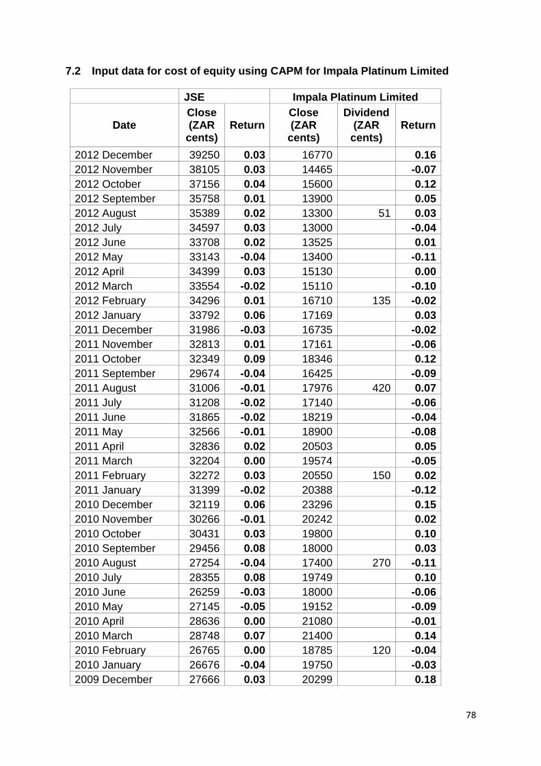
78

7.2 Input data for cost of equity using CAPM for Impala Platinum Limited

JSE Impala Platinum Limited

Date Close (ZAR

cents) Return

Close (ZAR

cents)

Dividend (ZAR

cents) Return

2012 December 39250 0.03 16770 0.16

2012 November 38105 0.03 14465 -0.07

2012 October 37156 0.04 15600 0.12

2012 September 35758 0.01 13900 0.05

2012 August 35389 0.02 13300 51 0.03

2012 July 34597 0.03 13000 -0.04

2012 June 33708 0.02 13525 0.01

2012 May 33143 -0.04 13400 -0.11

2012 April 34399 0.03 15130 0.00

2012 March 33554 -0.02 15110 -0.10

2012 February 34296 0.01 16710 135 -0.02

2012 January 33792 0.06 17169 0.03

2011 December 31986 -0.03 16735 -0.02

2011 November 32813 0.01 17161 -0.06

2011 October 32349 0.09 18346 0.12

2011 September 29674 -0.04 16425 -0.09

2011 August 31006 -0.01 17976 420 0.07

2011 July 31208 -0.02 17140 -0.06

2011 June 31865 -0.02 18219 -0.04

2011 May 32566 -0.01 18900 -0.08

2011 April 32836 0.02 20503 0.05

2011 March 32204 0.00 19574 -0.05

2011 February 32272 0.03 20550 150 0.02

2011 January 31399 -0.02 20388 -0.12

2010 December 32119 0.06 23296 0.15

2010 November 30266 -0.01 20242 0.02

2010 October 30431 0.03 19800 0.10

2010 September 29456 0.08 18000 0.03

2010 August 27254 -0.04 17400 270 -0.11

2010 July 28355 0.08 19749 0.10

2010 June 26259 -0.03 18000 -0.06

2010 May 27145 -0.05 19152 -0.09

2010 April 28636 0.00 21080 -0.01

2010 March 28748 0.07 21400 0.14

2010 February 26765 0.00 18785 120 -0.04

2010 January 26676 -0.04 19750 -0.03

2009 December 27666 0.03 20299 0.18

79

2009 November 26895 0.02 17175 -0.01

2009 October 26361 0.06 17430 0.00

2009 September 24911 0.00 17500 -0.04

2009 August 24929 0.03 18180 200 -0.02

2009 July 24259 0.10 18799 0.10

2009 June 22049 -0.03 17045 -0.12

2009 May 22771 0.10 19300 0.18

2009 April 20647 0.01 16385 0.04

2009 March 20364 0.10 15825 0.33

2009 February 18465 -0.10 11859 120 0.01

2009 January 20570 -0.04 11892 -0.12

2008 December 21509 0.01 13500 0.09

2008 November 21209 0.01 12400 0.23

2008 October 20992 -0.12 10090 -0.39

2008 September 23836 -0.14 16600 -0.24

2008 August 27702 0.00 21795 1175 -0.07

2008 July 27720 -0.09 24582 -0.20

2008 June 30413 -0.04 30900 -0.05

2008 May 31841 0.04 32501 0.06

2008 April 30743 0.04 30800 -0.02

2008 March 29588 -0.04 31300 -0.05

2008 February 30674 0.12 32806 300 0.19

2008 January 27317 -0.06 27800 0.17

2007 December 28958 -0.04 23725 0.00

2007 November 30308 -0.03 23686 -0.03

2007 October 31335 0.05 24400 0.02

2007 September 29959 0.05 24000 0.13

2007 August 28660 0.00 21210 700 0.04

2007 July 28562 0.01 21000 -0.03

2007 June 28337 -0.01 21600 -0.01

2007 May 28628 0.02 21801 -0.05

2007 April 28171 0.03 23000 0.01

2007 March 27267 0.06 22801 0.11

2007 February 25796 0.01 20600 275 0.01

2007 January 25448 0.02 20755 0.13

2006 December 24915 0.04 18400 0.02

2006 November 23950 0.03 18100 0.12

2006 October 23338 0.04 16187.5 0.01

2006 September 22375 0.02 16062.5 -0.04

2006 August 21954 0.05 16687.5 2200 0.18

2006 July 20886 -0.02 16000 -0.03

2006 June 21238 0.03 16497.75 0.16

2006 May 20565 -0.03 14187.5 0.00

80

2006 April 21136 0.04 14250 -0.02

2006 March 20352 0.07 14562.5 0.11

2006 February 19085 -0.03 13125 6500 0.50

2006 January 19745 0.09 13125 0.13

2005 December 18097 0.08 11650 0.10

2005 November 16775 0.02 10575 0.15

2005 October 16433 -0.03 9188.125 0.02

2005 September 16876 0.09 9037.5 0.08

2005 August 15414 0.02 8375.125 1800 0.34

2005 July 15144 0.07 7606.25 0.02

2005 June 14155 0.03 7462.5 0.05

2005 May 13787 0.10 7126.25 0.13

2005 April 12556 -0.06 6312.5 -0.04

2005 March 13299 -0.01 6562.5 0.03

2005 February 13477 0.05 6387.5 500 0.10

2005 January 12799 0.01 6245 0.04

2004 December 12657 0.01 5987.5 -0.03

2004 November 12491 0.07 6200 0.01

2004 October 11655 -0.01 6165 -0.05

2004 September 11761 0.05 6487.5 -0.07

2004 August 11160 0.08 6981.25 1600 0.38

2004 July 10306 0.02 6198.75 0.05

2004 June 10109 -0.03 5887.5 -0.02

2004 May 10414 0.00 5999.875 0.01

2004 April 10386 -0.03 5918.75 -0.08

2004 March 10693 -0.02 6445.625 -0.07

2004 February 10896 0.00 6900 500 0.03

2004 January 10849 0.04 7150 -0.01

2003 December 10387 0.07 7250 -0.03

2003 November 9729.6 0.00 7500 -0.05

2003 October 9765.3 0.09 7918.75 0.09

2003 September 8925.7 -0.03 7262.5 0.02

2003 August 9226.2 0.05 7124.875 1750 0.51

2003 July 8809.6 0.05 5874.875 0.05

2003 June 8352.2 -0.02 5575 -0.09

2003 May 8564.3 0.14 6125 0.36

2003 April 7510.4 -0.02 4500 -0.10

2003 March 7679.9 -0.09 5012.5 -0.18

2003 February 8402.1 -0.05 6127.5 900 -0.05

2003 January 8798.4 -0.05 7387.5 0.08

2002 December 9277.2 -0.03 6812.5 -0.04

2002 November 9563.7 0.02 7075 -0.02

2002 October 9376.2 -0.01 7187.5 0.03

81

2002 September 9465.3 -0.02 7002.5 0.05

2002 August 9677.3 0.05 6675 2600 0.73

2002 July 9239 -0.13 5350 -0.25

2002 June 10658 -0.05 7147.5 -0.11

2002 May 11201 0.02 7995 -0.07

2002 April 11008 0.00 8625 0.14

2002 March 11015 0.01 7537.5 0.02

2002 February 10875 0.05 7425 1100 0.32

2002 January 10334 -0.01 6460 -0.08

2001 December 10456 0.11 7030 0.31

2001 November 9404.1 0.11 5375 0.28

2001 October 8473.5 0.06 4195 0.06

2001 September 7997.9 -0.10 3975 -0.13

2001 August 8886.7 0.05 4575 2380 0.57

2001 July 8456 -0.07 4425 -0.12

2001 June 9089.9 -0.02 5042.5 -0.15

2001 May 9270.8 0.04 5912.5 0.23

2001 April 8902.3 0.10 4812.5 0.35

2001 March 8093.8 -0.09 3562.5 -0.32

2001 February 8916.3 0.00 5247.5 7420 1.59

2001 January 8942.4 0.10 4897.5 0.02

2000 December 8164.3 0.06 4822.5 0.06

2000 November 7687.1 -0.04 4552.5 0.12

2000 October 8026.4 -0.01 4050 0.04

2000 September 8146.8 -0.03 3902.5 -0.05

2000 August 8361.6 0.10 4125 1420 0.67

2000 July 7621.7 0.01 3317.5 0.05

2000 June 7570.4 0.05 3152.5 0.08

2000 May 7175.9 -0.01 2907.5 0.08

2000 April 7250.2 -0.07 2687.5 -0.05

2000 March 7765.4 0.00 2837.5 0.00

2000 February 7733.2 -0.06 2827.5 340 -0.08

2000 January 8249.4 -0.01 3450 0.11

1999 December 8357.2 0.13 3112.5 0.11

1999 November 7405.9 0.07 2812.5 0.06

1999 October 6948.9 0.05 2660 0.03

1999 September 6629 -0.01 2587.5 0.06

1999 August 6673.2 -0.02 2437.5 710 0.28

1999 July 6822.7 0.02 2452.5 0.29

1999 June 6721.2 0.09 1897.5 0.01

1999 May 6146.7 -0.08 1887.5 0.09

1999 April 6678.4 0.12 1730 0.31

1999 March 5973.4 0.08 1325 -0.05

82

1999 February 5543.5 0.02 1390 170 0.31

1999 January 5414.8 0.08 1187.5 0.19

1998 December 5015.7 -0.04 1000 0.02

1998 November 5200.2 -0.03 976.25 0.28

1998 October 5350.8 0.14 763.75 -0.16

1998 September 4702.6 0.05 906.25 0.19

1998 August 4479.9 -0.29 762.5 290 0.22

1998 July 6350.3 0.05 862.5 0.37

1998 June 6035.6 -0.11 631.25 -0.08

1998 May 6795.3 -0.08 687.5 -0.16

1998 April 7392.7 0.10 821.25 0.17

1998 March 6749.2 0.07 700 0.14

1998 February 6283.1 0.08 612.5 60 0.14

1998 January 5830.3 0.07 587.5 0.01

1997 December 5465.6 581.25

83

7.3 Input data for cost of equity using CAPM for Lonmin

JSE Lonmin Plc

Date Close (ZAR

cents) Return

Close (ZAR cents)

Dividend (ZAR

cents) Return

2012 December 39250.24 0.03 3891 0.05

2012 November 38104.61 0.03 3720 -0.49

2012 October 37156.28 0.04 7250 -0.03

2012 September 35757.98 0.01 7470 -0.04

2012 August 35389.45 0.02 7745 -0.14

2012 July 34596.9 0.03 9043 -0.09

2012 June 33708.31 0.02 9972 0.07

2012 May 33142.61 -0.04 9330 -0.29

2012 April 34399.04 0.03 13180 0.05

2012 March 33554.21 -0.02 12580 -0.06

2012 February 34296 0.01 13450 0.04

2012 January 33792.48 0.06 12989 0.06

2011 December 31985.67 -0.03 12200 -0.10

2011 November 32812.64 0.01 13628 122 -0.02

2011 October 32348.54 0.09 14076 0.07

2011 September 29674.2 -0.04 13140 -0.12

2011 August 31005.5 -0.01 15000 0.07

2011 July 31208.04 -0.02 14068 -0.11

2011 June 31864.54 -0.02 15800 -0.12

2011 May 32565.73 -0.01 18000 0.00

2011 April 32836.23 0.02 18002 -0.04

2011 March 32204.06 0.00 18750 -0.10

2011 February 32272.09 0.03 20845 0.09

2011 January 31398.75 -0.02 19111 -0.06

2010 December 32118.89 0.06 20400 0.09

2010 November 30266.4 -0.01 18723 99 -0.04

2010 October 30430.9 0.03 19550 0.05

2010 September 29456.04 0.08 18700 0.08

2010 August 27253.87 -0.04 17300 -0.05

2010 July 28355.21 0.08 18150 0.11

2010 June 26258.82 -0.03 16300 -0.13

2010 May 27145.36 -0.05 18817 -0.13

2010 April 28635.76 0.00 21582 -0.05

2010 March 28747.56 0.07 22625 0.07

2010 February 26764.61 0.00 21079 -0.05

2010 January 26675.95 -0.04 22150 -0.05

2009 December 27666.45 0.03 23200 0.07

2009 November 26894.74 0.02 21650 0.12

2009 October 26360.55 0.06 19250 -0.04

2009 September 24910.85 0.00 20001 0.10

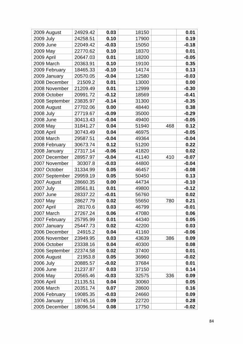
84

2009 August 24929.42 0.03 18150 0.01

2009 July 24258.51 0.10 17900 0.19

2009 June 22049.42 -0.03 15050 -0.18

2009 May 22770.62 0.10 18370 0.01

2009 April 20647.03 0.01 18200 -0.05

2009 March 20363.91 0.10 19100 0.35

2009 February 18465.33 -0.10 14174 0.13

2009 January 20570.05 -0.04 12580 -0.03

2008 December 21509.2 0.01 13000 0.00

2008 November 21209.49 0.01 12999 -0.30

2008 October 20991.72 -0.12 18569 -0.41

2008 September 23835.97 -0.14 31300 -0.35

2008 August 27702.06 0.00 48440 0.38

2008 July 27719.67 -0.09 35000 -0.29

2008 June 30413.43 -0.04 49400 -0.05

2008 May 31841.27 0.04 51940 468 0.12

2008 April 30743.49 0.04 46975 -0.05

2008 March 29587.51 -0.04 49364 -0.04

2008 February 30673.74 0.12 51200 0.22

2008 January 27317.14 -0.06 41820 0.02

2007 December 28957.97 -0.04 41140 410 -0.07

2007 November 30307.8 -0.03 44800 -0.04

2007 October 31334.99 0.05 46457 -0.08

2007 September 29959.19 0.05 50450 0.13

2007 August 28660.35 0.00 44734 -0.10

2007 July 28561.81 0.01 49800 -0.12

2007 June 28337.22 -0.01 56760 0.02

2007 May 28627.79 0.02 55650 780 0.21

2007 April 28170.6 0.03 46799 -0.01

2007 March 27267.24 0.06 47080 0.06

2007 February 25795.99 0.01 44340 0.05

2007 January 25447.73 0.02 42200 0.03

2006 December 24915.2 0.04 41160 -0.06

2006 November 23949.95 0.03 43639 386 0.09

2006 October 23338.16 0.04 40300 0.08

2006 September 22374.58 0.02 37400 0.01

2006 August 21953.8 0.05 36960 -0.02

2006 July 20885.57 -0.02 37684 0.01

2006 June 21237.87 0.03 37150 0.14

2006 May 20565.46 -0.03 32575 336 0.09

2006 April 21135.51 0.04 30060 0.05

2006 March 20351.74 0.07 28600 0.16

2006 February 19085.35 -0.03 24660 0.09

2006 January 19745.16 0.09 22720 0.28

2005 December 18096.54 0.08 17750 -0.02

85

2005 November 16774.54 0.02 18101 266 0.20

2005 October 16433.1 -0.03 15325 0.04

2005 September 16875.65 0.09 14700 0.07

2005 August 15414.01 0.02 13700 0.03

2005 July 15143.64 0.07 13295 0.06

2005 June 14154.73 0.03 12500 0.00

2005 May 13787.02 0.10 12500 203 0.14

2005 April 12555.96 -0.06 11100 -0.03

2005 March 13298.58 -0.01 11500 0.04

2005 February 13476.59 0.05 11050 0.03

2005 January 12798.55 0.01 10700 0.08

2004 December 12656.86 0.01 9900 253 -0.06

2004 November 12490.79 0.07 10750 277 -0.07

2004 October 11655.31 -0.01 11800 -0.10

2004 September 11761 0.05 13040 0.02

2004 August 11160.44 0.08 12800 0.16

2004 July 10305.89 0.02 11000 -0.03

2004 June 10108.61 -0.03 11374 0.01

2004 May 10413.81 0.00 11300 188 -0.05

2004 April 10385.8 -0.03 12100 -0.09

2004 March 10692.56 -0.02 13300 -0.11

2004 February 10895.86 0.00 14950 0.03

2004 January 10849.25 0.04 14491 0.11

2003 December 10387.22 0.07 13000 278 0.11

2003 November 9729.6 0.00 11950 0.01

2003 October 9765.3 0.09 11825 0.11

2003 September 8925.69 -0.03 10650 -0.01

2003 August 9226.2 0.05 10749 0.07

2003 July 8809.63 0.05 10000 0.03

2003 June 8352.2 -0.02 9700 -0.11

2003 May 8564.33 0.14 10940 226 0.39

2003 April 7510.4 -0.02 8025 -0.05

2003 March 7679.88 -0.09 8480 -0.16

2003 February 8402.09 -0.05 10100 -0.05

2003 January 8798.35 -0.05 10600 -0.12

2002 December 9277.22 -0.03 12000 -0.02

2002 November 9563.74 0.02 12300 358 -0.08

2002 October 9376.23 -0.01 13750 -0.02

2002 September 9465.33 -0.02 14100 0.00

2002 August 9677.26 0.05 14100 0.01

2002 July 9239.02 -0.13 14000 -0.23

2002 June 10657.73 -0.05 18172 0.07

2002 May 11200.85 0.02 17010 302 -0.04

2002 April 11007.67 0.00 18000 -0.07

2002 March 11015.04 0.01 19380 0.02

86

2002 February 10875.09 0.05 19000 0.02

2002 January 10333.52 -0.01 18690.47619 -0.10

2001 December 10456.47 0.11 20833.33333 5763 0.58

2001 November 9404.06 0.11 16833.33333 0.31

2001 October 8473.51 0.06 12857.14286 -0.01

2001 September 7997.87 -0.10 12976.19048 -0.03

2001 August 8886.72 0.05 13309.52381 0.10

2001 July 8456.01 -0.07 12095.2381 -0.12

2001 June 9089.89 -0.02 13761.90476 -0.02

2001 May 9270.84 0.04 14095.2381 0.08

2001 April 8902.33 0.10 13095.2381 0.09

2001 March 8093.79 -0.09 12023.80952 -0.13

2001 February 8916.29 0.00 13809.52381 -0.03

2001 January 8942.37 0.10 14285.71429 0.11

2000 December 8164.29 0.06 12857.14286 0.04

2000 November 7687.08 -0.04 12380.95238 260 0.17

2000 October 8026.39 -0.01 10833.33333 0.01

2000 September 8146.75 -0.03 10773.80952 0.03

2000 August 8361.62 0.10 10476.19048 0.01

2000 July 7621.68 0.01 10333.33333 0.13

2000 June 7570.39 0.05 9166.66667 97 0.20

2000 May 7175.9 -0.01 7738.09524 -0.07

2000 April 7250.19 -0.07 8333.33333 0.05

2000 March 7765.41 0.00 7940.47619 0.00

2000 February 7733.24 -0.06 7976.19048 -0.04

2000 January 8249.35 -0.01 8321.42857 114 0.13

1999 December 8357.19 0.13 7440.47619 0.12

1999 November 7405.91 0.07 6666.66667 -0.08

1999 October 6948.86 0.05 7261.90476 -0.02

1999 September 6628.98 -0.01 7416.66667 0.12

1999 August 6673.17 -0.02 6642.85714 -0.10

1999 July 6822.68 0.02 7392.85714 75 0.12

1999 June 6721.15 0.09 6666.66667 0.18

1999 May 6146.74 -0.08 5654.7619 -0.10

1999 April 6678.44 0.12 6250 0.17

1999 March 5973.43 0.08 5357.14286 0.12

1999 February 5543.5 0.02 4785.71429 0.20

1999 January 5414.79 0.08 3988.09524 98 0.07

1998 December 5015.72 -0.04 3815.47619 0.05

1998 November 5200.18 -0.03 3619.04762 -0.02

1998 October 5350.76 0.14 3690.47619 -0.02

1998 September 4702.59 0.05 3750 0.27

1998 August 4479.85 -0.29 2952.38095 -0.10

1998 July 6350.31 0.05 3273.80952 0.01

1998 June 6035.63 -0.11 3238.09524 141 0.13

87

1998 May 6795.3 -0.08 2982.14286 -0.31

1998 April 7392.66 0.10 4333.33333 -0.01

1998 March 6749.22 0.07 4357.14286 0.19

1998 February 6283.14 0.08 3666.66667 0.00

1998 January 5830.29 0.07 3666.66667 14 0.04

1997 December 5465.6 3523.80952

88

7.4 Input data for cost of equity using CAPM for AngloGold Ashanti

JSE Anglo Gold Ashanti Limited

Date Close (ZAR

cents) Return

Close (ZAR

cents)

Dividend (ZAR

cents) Return

2012 December 39250.24 0.03 26234.00 -0.06

2012 November 38104.61 0.03 27808.00 42.5 -0.03

2012 October 37156.28 0.04 28847.00 -0.01

2012 September 35757.98 0.01 29242.00 0.11

2012 August 35389.45 0.02 26289.00 85 -0.07

2012 July 34596.9 0.03 28290.00 0.01

2012 June 33708.31 0.02 27900.00 -0.10

2012 May 33142.61 -0.04 30850.00 85 0.17

2012 April 34399.04 0.03 26458.00 -0.06

2012 March 33554.21 -0.02 28240.00 -0.13

2012 February 34296 0.01 32574.00 200 -0.09

2012 January 33792.48 0.06 35900.00 0.05

2011 December 31985.67 -0.03 34340.00 -0.11

2011 November 32812.64 0.01 38440.00 90 0.07

2011 October 32348.54 0.09 35850.00 0.06

2011 September 29674.2 -0.04 33890.00 0.07

2011 August 31005.5 -0.01 31800.00 90 0.13

2011 July 31208.04 -0.02 28100.00 -0.02

2011 June 31864.54 -0.02 28550.00 -0.09

2011 May 32565.73 -0.01 31400.00 -0.06

2011 April 32836.23 0.02 33278.00 0.03

2011 March 32204.06 0.00 32450.00 -0.04

2011 February 32272.09 0.03 33949.00 80 0.11

2011 January 31398.75 -0.02 30637.00 -0.06

2010 December 32118.89 0.06 32690.00 0.00

2010 November 30266.4 -0.01 32837.00 0.01

2010 October 30430.9 0.03 32649.00 0.01

2010 September 29456.04 0.08 32335.00 0.02

2010 August 27253.87 -0.04 31640.00 65 0.08

2010 July 28355.21 0.08 29480.00 -0.11

2010 June 26258.82 -0.03 33195.00 0.01

2010 May 27145.36 -0.05 32799.00 0.05

2010 April 28635.76 0.00 31149.00 0.12

2010 March 28747.56 0.07 27795.00 0.00

2010 February 26764.61 0.00 27699.00 70 0.00

2010 January 26675.95 -0.04 27895.00 -0.09

2009 December 27666.45 0.03 30629.00 -0.05

2009 November 26894.74 0.02 32401.00 0.12

2009 October 26360.55 0.06 28990.00 -0.04

89

2009 September 24910.85 0.00 30150.00 0.01

2009 August 24929.42 0.03 29805.00 0.01

2009 July 24258.51 0.10 29600.00 60 0.05

2009 June 22049.42 -0.03 28302.00 -0.18

2009 May 22770.62 0.10 34600.00 0.32

2009 April 20647.03 0.01 26180.00 -0.24

2009 March 20363.91 0.10 34500.00 0.16

2009 February 18465.33 -0.10 29750.00 50 0.04

2009 January 20570.05 -0.04 28625.00 0.14

2008 December 21509.2 0.01 25200.00 0.15

2008 November 21209.49 0.01 21900.00 0.16

2008 October 20991.72 -0.12 18849.00 -0.02

2008 September 23835.97 -0.14 19200.00 -0.08

2008 August 27702.06 0.00 20850.00 50 -0.13

2008 July 27719.67 -0.09 24125.00 -0.10

2008 June 30413.43 -0.04 26885.00 -0.06

2008 May 31841.27 0.04 28650.00 0.13

2008 April 30743.49 0.04 25300.00 -0.07

2008 March 29587.51 -0.04 27201.00 -0.04

2008 February 30673.74 0.12 28350.00 53 -0.09

2008 January 27317.14 -0.06 31190.00 0.06

2007 December 28957.97 -0.04 29300.00 -0.13

2007 November 30307.8 -0.03 33800.00 0.11

2007 October 31334.99 0.05 30399.00 -0.07

2007 September 29959.19 0.05 32620.00 0.17

2007 August 28660.35 0.00 27921.00 -0.07

2007 July 28561.81 0.01 30122.00 90 0.13

2007 June 28337.22 -0.01 26710.00 -0.09

2007 May 28627.79 0.02 29205.00 -0.07

2007 April 28170.6 0.03 31531.00 -0.03

2007 March 27267.24 0.06 32500.00 0.03

2007 February 25795.99 0.01 31500.00 240 -0.07

2007 January 25447.73 0.02 34200.00 0.04

2006 December 24915.2 0.04 32999.00 -0.04

2006 November 23949.95 0.03 34350.00 0.10

2006 October 23338.16 0.04 31260.00 0.07

2006 September 22374.58 0.02 29120.00 -0.11

2006 August 21953.8 0.05 32689.00 -0.01

2006 July 20885.57 -0.02 33175.00 210 -0.06

2006 June 21237.87 0.03 35499.00 0.15

2006 May 20565.46 -0.03 30900.00 -0.05

2006 April 21135.51 0.04 32601.00 -0.01

2006 March 20351.74 0.07 32800.00 0.03

2006 February 19085.35 -0.03 31801.00 62 -0.14

2006 January 19745.16 0.09 37100.00 0.18

90

2005 December 18096.54 0.08 31400.00 0.13

2005 November 16774.54 0.02 27845.00 0.04

2005 October 16433.1 -0.03 26750.00 -0.03

2005 September 16875.65 0.09 27590.00 0.22

2005 August 15414.01 0.02 22650.00 0.00

2005 July 15143.64 0.07 22703.00 170 -0.04

2005 June 14154.73 0.03 23950.00 0.06

2005 May 13787.02 0.10 22599.00 0.16

2005 April 12555.96 -0.06 19500.00 -0.10

2005 March 13298.58 -0.01 21600.00 0.04

2005 February 13476.59 0.05 20800.00 0.06

2005 January 12798.55 0.01 19569.00 180 -0.01

2004 December 12656.86 0.01 19901.00 -0.15

2004 November 12490.79 0.07 23345.00 0.03

2004 October 11655.31 -0.01 22650.00 -0.09

2004 September 11761 0.05 24922.00 0.06

2004 August 11160.44 0.08 23500.00 0.14

2004 July 10305.89 0.02 20660.00 170 0.03

2004 June 10108.61 -0.03 20249.00 -0.11

2004 May 10413.81 0.00 22800.00 0.03

2004 April 10385.8 -0.03 22100.00 -0.18

2004 March 10692.56 -0.02 26960.00 -0.04

2004 February 10895.86 0.00 28200.00 -0.02

2004 January 10849.25 0.04 28702.00 335 -0.08

2003 December 10387.22 0.07 31399.00 0.02

2003 November 9729.6 0.00 30639.00 0.15

2003 October 9765.3 0.09 26660.00 -0.01

2003 September 8925.69 -0.03 26900.00 -0.05

2003 August 9226.2 0.05 28400.00 0.17

2003 July 8809.63 0.05 24350.00 375 0.04

2003 June 8352.2 -0.02 23700.00 0.04

2003 May 8564.33 0.14 22710.00 0.09

2003 April 7510.4 -0.02 20750.00 -0.12

2003 March 7679.88 -0.09 23660.00 -0.09

2003 February 8402.09 -0.05 25869.00 -0.14

2003 January 8798.35 -0.05 30000.00 675 0.06

2002 December 9277.22 -0.03 29050.00 0.19

2002 November 9563.74 0.02 24472.36 -0.07

2002 October 9376.23 -0.01 26221.11 -0.08

2002 September 9465.33 -0.02 28628.14 0.16

2002 August 9677.26 0.05 24623.12 0.11

2002 July 9239.02 -0.13 22160.80 1350 -0.15

2002 June 10657.73 -0.05 27537.69 -0.13

2002 May 11200.85 0.02 31608.04 0.09

2002 April 11007.67 0.00 29045.23 0.01

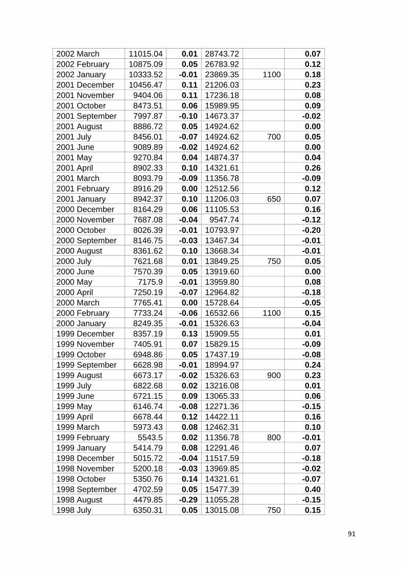
91

2002 March 11015.04 0.01 28743.72 0.07

2002 February 10875.09 0.05 26783.92 0.12

2002 January 10333.52 -0.01 23869.35 1100 0.18

2001 December 10456.47 0.11 21206.03 0.23

2001 November 9404.06 0.11 17236.18 0.08

2001 October 8473.51 0.06 15989.95 0.09

2001 September 7997.87 -0.10 14673.37 -0.02

2001 August 8886.72 0.05 14924.62 0.00

2001 July 8456.01 -0.07 14924.62 700 0.05

2001 June 9089.89 -0.02 14924.62 0.00

2001 May 9270.84 0.04 14874.37 0.04

2001 April 8902.33 0.10 14321.61 0.26

2001 March 8093.79 -0.09 11356.78 -0.09

2001 February 8916.29 0.00 12512.56 0.12

2001 January 8942.37 0.10 11206.03 650 0.07

2000 December 8164.29 0.06 11105.53 0.16

2000 November 7687.08 -0.04 9547.74 -0.12

2000 October 8026.39 -0.01 10793.97 -0.20

2000 September 8146.75 -0.03 13467.34 -0.01

2000 August 8361.62 0.10 13668.34 -0.01

2000 July 7621.68 0.01 13849.25 750 0.05

2000 June 7570.39 0.05 13919.60 0.00

2000 May 7175.9 -0.01 13959.80 0.08

2000 April 7250.19 -0.07 12964.82 -0.18

2000 March 7765.41 0.00 15728.64 -0.05

2000 February 7733.24 -0.06 16532.66 1100 0.15

2000 January 8249.35 -0.01 15326.63 -0.04

1999 December 8357.19 0.13 15909.55 0.01

1999 November 7405.91 0.07 15829.15 -0.09

1999 October 6948.86 0.05 17437.19 -0.08

1999 September 6628.98 -0.01 18994.97 0.24

1999 August 6673.17 -0.02 15326.63 900 0.23

1999 July 6822.68 0.02 13216.08 0.01

1999 June 6721.15 0.09 13065.33 0.06

1999 May 6146.74 -0.08 12271.36 -0.15

1999 April 6678.44 0.12 14422.11 0.16

1999 March 5973.43 0.08 12462.31 0.10

1999 February 5543.5 0.02 11356.78 800 -0.01

1999 January 5414.79 0.08 12291.46 0.07

1998 December 5015.72 -0.04 11517.59 -0.18

1998 November 5200.18 -0.03 13969.85 -0.02

1998 October 5350.76 0.14 14321.61 -0.07

1998 September 4702.59 0.05 15477.39 0.40

1998 August 4479.85 -0.29 11055.28 -0.15

1998 July 6350.31 0.05 13015.08 750 0.15

92

1998 June 6035.63 -0.11 12010.05 -0.07

1998 May 6795.3 -0.08 12864.32 -0.04

1998 April 7392.66 0.10 13467.34 0.28

1998 March 6749.22 0.07 10482.41 0.03

1998 February 6283.14 0.08 10201.01 -0.12

1998 January 5830.29 0.07 11608.04 875 0.27

1997 December 5465.6 9798.99

93

7.5 Input data for cost of equity using CAPM for Gold Fields

JSE Gold Fields Limited

Date Close (ZAR

cents) Return

Close (ZAR

cents)

Dividend (ZAR

cents) Return

2012 December 39250 0.03 10375 -0.06

2012 November 38105 0.03 11021 0.03

2012 October 37156 0.04 10705 0.00

2012 September 35758 0.01 10675 0.06

2012 August 35389 0.02 10103 159 -0.04

2012 July 34597 0.03 10714 0.03

2012 June 33708 0.02 10385 -0.09

2012 May 33143 -0.04 11419 0.15

2012 April 34399 0.03 9890 -0.06

2012 March 33554 -0.02 10500 -0.12

2012 February 34296 0.01 11880 230 -0.06

2012 January 33792 0.06 12900 0.04

2011 December 31986 -0.03 12460 -0.09

2011 November 32813 0.01 13651 -0.01

2011 October 32349 0.09 13720 0.10

2011 September 29674 -0.04 12486 0.07

2011 August 31006 -0.01 11700 100 0.14

2011 July 31208 -0.02 10360 0.04

2011 June 31865 -0.02 9919 -0.12

2011 May 32566 -0.01 11300 -0.04

2011 April 32836 0.02 11728 -0.01

2011 March 32204 0.00 11845 -0.05

2011 February 32272 0.03 12479 70 0.11

2011 January 31399 -0.02 11284 -0.06

2010 December 32119 0.06 12060 0.04

2010 November 30266 -0.01 11566 0.06

2010 October 30431 0.03 10962 0.04

2010 September 29456 0.08 10560 0.00

2010 August 27254 -0.04 10600 70 0.08

2010 July 28355 0.08 9835 -0.05

2010 June 26259 -0.03 10380 -0.04

2010 May 27145 -0.05 10774 0.09

2010 April 28636 0.00 9868 0.07

2010 March 28748 0.07 9220 0.04

2010 February 26765 0.00 8885 50 0.00

2010 January 26676 -0.04 8905 -0.09

94

2009 December 27666 0.03 9798 -0.09

2009 November 26895 0.02 10810 0.08

2009 October 26361 0.06 10050 -0.01

2009 September 24911 0.00 10150 0.07

2009 August 24929 0.03 9473 80 0.03

2009 July 24259 0.10 9245 -0.01

2009 June 22049 -0.03 9352 -0.15

2009 May 22771 0.10 11001 0.25

2009 April 20647 0.01 8835 -0.15

2009 March 20364 0.10 10450 0.00

2009 February 18465 -0.10 10450 -0.04

2009 January 20570 -0.04 10839 30 0.18

2008 December 21509 0.01 9190 0.10

2008 November 21209 0.01 8370 0.21

2008 October 20992 -0.12 6900 -0.14

2008 September 23836 -0.14 8050 0.13

2008 August 27702 0.00 7100 120 -0.18

2008 July 27720 -0.09 8847 -0.11

2008 June 30413 -0.04 9950 0.02

2008 May 31841 0.04 9775 65 -0.02

2008 April 30743 0.04 10000 -0.13

2008 March 29588 -0.04 11500 0.05

2008 February 30674 0.12 10950 -0.02

2008 January 27317 -0.06 11219 0.13

2007 December 28958 -0.04 9900 -0.14

2007 November 30308 -0.03 11509 -0.02

2007 October 31335 0.05 11688 -0.06

2007 September 29959 0.05 12415 0.13

2007 August 28660 0.00 10950 95 -0.06

2007 July 28562 0.01 11739 0.07

2007 June 28337 -0.01 10940 -0.09

2007 May 28628 0.02 12052 -0.06

2007 April 28171 0.03 12801 -0.05

2007 March 27267 0.06 13450 0.08

2007 February 25796 0.01 12496 0.03

2007 January 25448 0.02 12121 90 -0.08

2006 December 24915 0.04 13275 0.00

2006 November 23950 0.03 13285 0.09

2006 October 23338 0.04 12200 -0.11

2006 September 22375 0.02 13749 -0.02

2006 August 21954 0.05 14000 110 -0.01

2006 July 20886 -0.02 14311 -0.12

2006 June 21238 0.03 16200 0.10

95

2006 May 20565 -0.03 14750 -0.02

2006 April 21136 0.04 15126 0.13

2006 March 20352 0.07 13439 0.00

2006 February 19085 -0.03 13500 -0.05

2006 January 19745 0.09 14200 40 0.27

2005 December 18097 0.08 11180 0.13

2005 November 16775 0.02 9925 0.10

2005 October 16433 -0.03 9030 -0.05

2005 September 16876 0.09 9532 0.29

2005 August 15414 0.02 7370 40 0.03

2005 July 15144 0.07 7199 -0.06

2005 June 14155 0.03 7620 0.03

2005 May 13787 0.10 7401 0.21

2005 April 12556 -0.06 6100 -0.16

2005 March 13299 -0.01 7250 0.05

2005 February 13477 0.05 6905 30 0.01

2005 January 12799 0.01 6840 -0.02

2004 December 12657 0.01 6950 -0.15

2004 November 12491 0.07 8220 -0.04

2004 October 11655 -0.01 8601 -0.02

2004 September 11761 0.05 8750 0.08

2004 August 11160 0.08 8075 0.25

2004 July 10306 0.02 6461 40 0.00

2004 June 10109 -0.03 6531 -0.15

2004 May 10414 0.00 7709 0.10

2004 April 10386 -0.03 7025 -0.17

2004 March 10693 -0.02 8425 0.03

2004 February 10896 0.00 8200 -0.10

2004 January 10849 0.04 9101 40 -0.04

2003 December 10387 0.07 9550 0.09

2003 November 9730 0.00 8800 -0.11

2003 October 9765 0.09 9851 -0.01

2003 September 8926 -0.03 9970 0.00

2003 August 9226 0.05 10000 100 0.13

2003 July 8810 0.05 8920 0.00

2003 June 8352 -0.02 8957 0.00

2003 May 8564 0.14 9000 0.22

2003 April 7510 -0.02 7390 -0.12

2003 March 7680 -0.09 8420 -0.17

2003 February 8402 -0.05 10100 -0.09

2003 January 8798 -0.05 11130 150 -0.06

2002 December 9277 -0.03 11990 0.21

2002 November 9564 0.02 9950 -0.13

96

2002 October 9376 -0.01 11461 -0.16

2002 September 9465 -0.02 13599 0.09

2002 August 9677 0.05 12520 220 0.17

2002 July 9239 -0.13 10900 -0.11

2002 June 10658 -0.05 12180 -0.06

2002 May 11201 0.02 12950 0.01

2002 April 11008 0.00 12820 0.08

2002 March 11015 0.01 11880 0.20

2002 February 10875 0.05 9880 90 0.38

2002 January 10334 -0.01 7240 0.26

2001 December 10456 0.11 5750 0.22

2001 November 9404 0.11 4720 0.10

2001 October 8474 0.06 4280 0.05

2001 September 7998 -0.10 4070 0.12

2001 August 8887 0.05 3620 40 0.09

2001 July 8456 -0.07 3370 -0.07

2001 June 9090 -0.02 3625 0.09

2001 May 9271 0.04 3340 -0.05

2001 April 8902 0.10 3505 0.12

2001 March 8094 -0.09 3120 -0.01

2001 February 8916 0.00 3150 105 0.11

2001 January 8942 0.10 2920 0.14

2000 December 8164 0.06 2570 0.18

2000 November 7687 -0.04 2180 -0.02

2000 October 8026 -0.01 2235 -0.02

2000 September 8147 -0.03 2290 -0.11

2000 August 8362 0.10 2570 0.06

2000 July 7622 0.01 2430 -0.09

2000 June 7570 0.05 2660 0.06

2000 May 7176 -0.01 2520 0.15

2000 April 7250 -0.07 2200 -0.04

2000 March 7765 0.00 2280 -0.22

2000 February 7733 -0.06 2940 20 0.15

2000 January 8249 -0.01 2580 -0.13

1999 December 8357 0.13 2975 0.07

1999 November 7406 0.07 2775 -0.06

1999 October 6949 0.05 2940 0.06

1999 September 6629 -0.01 2775 0.32

1999 August 6673 -0.02 2100 30 0.19

1999 July 6823 0.02 1785 -0.14

1999 June 6721 0.09 2070 0.06

1999 May 6147 -0.08 1960 -0.20

1999 April 6678 0.12 2450 0.02

97

1999 March 5973 0.08 2400 0.05

1999 February 5544 0.02 2290 -0.16

1999 January 5415 0.08 2725 75 0.19

1998 December 5016 -0.04 2350 -0.25

1998 November 5200 -0.03 3125 -0.10

1998 October 5351 0.14 3475 0.12

1998 September 4703 0.05 3100 0.24

1998 August 4480 -0.29 2500 -0.14

1998 July 6350 0.05 2905 60 -0.03

1998 June 6036 -0.11 3070 -0.07

1998 May 6795 -0.08 3310 -0.08

1998 April 7393 0.10 3585 0.10

1998 March 6749 0.07 3250 0.02

1998 February 6283 0.08 3175 -0.02

1998 January 5830 0.07 3225 -0.02

1997 December 5466 3300 30

98

7.6 Input data for cost of equity using CAPM for Harmony

JSE Harmony Gold Mining

Company Limited

Date Close (ZAR

cents) Return

Close (ZAR

cents)

Dividend (ZAR

cents) Return

2012 December 39250 0.03 7400 0.06

2012 November 38105 0.03 6994 -0.02

2012 October 37156 0.04 7102 0.02

2012 September 35758 0.01 6983 0.02

2012 August 35389 0.02 6824 48 -0.17

2012 July 34597 0.03 8263 0.08

2012 June 33708 0.02 7650 -0.09

2012 May 33143 -0.04 8451 0.12

2012 April 34399 0.03 7564 -0.09

2012 March 33554 -0.02 8339 -0.16

2012 February 34296 0.01 9900 40 0.05

2012 January 33792 0.06 9511 0.00

2011 December 31986 -0.03 9500 -0.17

2011 November 32813 0.01 11437 0.09

2011 October 32349 0.09 10451 0.10

2011 September 29674 -0.04 9535 0.00

2011 August 31006 -0.01 9499 60 0.05

2011 July 31208 -0.02 9075 0.01

2011 June 31865 -0.02 8995 -0.05

2011 May 32566 -0.01 9475 -0.04

2011 April 32836 0.02 9915 0.00

2011 March 32204 0.00 9929 0.22

2011 February 32272 0.03 8123 0.04

2011 January 31399 -0.02 7800 -0.06

2010 December 32119 0.06 8300 0.05

2010 November 30266 -0.01 7895 -0.02

2010 October 30431 0.03 8020 0.03

2010 September 29456 0.08 7800 0.02

2010 August 27254 -0.04 7646 50 0.05

2010 July 28355 0.08 7305 -0.10

2010 June 26259 -0.03 8140 0.06

2010 May 27145 -0.05 7709 0.07

2010 April 28636 0.00 7210 0.05

2010 March 28748 0.07 6880 0.00

2010 February 26765 0.00 6905 -0.04

99

2010 January 26676 -0.04 7200 -0.05

2009 December 27666 0.03 7579 -0.08

2009 November 26895 0.02 8200 0.04

2009 October 26361 0.06 7850 -0.02

2009 September 24911 0.00 8000 0.10

2009 August 24929 0.03 7299 50 0.05

2009 July 24259 0.10 7020 -0.12

2009 June 22049 -0.03 8000 -0.18

2009 May 22771 0.10 9719 0.23

2009 April 20647 0.01 7901 -0.21

2009 March 20364 0.10 10041 -0.18

2009 February 18465 -0.10 12275 0.02

2009 January 20570 -0.04 12045 0.23

2008 December 21509 0.01 9770 0.14

2008 November 21209 0.01 8600 0.17

2008 October 20992 -0.12 7370 -0.11

2008 September 23836 -0.14 8275 0.23

2008 August 27702 0.00 6750 -0.16

2008 July 27720 -0.09 8025 -0.16

2008 June 30413 -0.04 9500 0.05

2008 May 31841 0.04 9050 0.05

2008 April 30743 0.04 8630 -0.11

2008 March 29588 -0.04 9725 0.01

2008 February 30674 0.12 9620 0.29

2008 January 27317 -0.06 7450 0.06

2007 December 28958 -0.04 7046 -0.03

2007 November 30308 -0.03 7300 -0.01

2007 October 31335 0.05 7355 -0.10

2007 September 29959 0.05 8159 0.27

2007 August 28660 0.00 6410 -0.35

2007 July 28562 0.01 9825 -0.02

2007 June 28337 -0.01 10027 -0.03

2007 May 28628 0.02 10388 -0.08

2007 April 28171 0.03 11297 0.12

2007 March 27267 0.06 10125 0.05

2007 February 25796 0.01 9679 -0.01

2007 January 25448 0.02 9797 -0.12

2006 December 24915 0.04 11120 -0.08

2006 November 23950 0.03 12126 0.09

2006 October 23338 0.04 11169 0.11

2006 September 22375 0.02 10059 0.03

2006 August 21954 0.05 9800 -0.01

2006 July 20886 -0.02 9850 -0.14

100

2006 June 21238 0.03 11410 0.21

2006 May 20565 -0.03 9420 -0.05

2006 April 21136 0.04 9900 -0.01

2006 March 20352 0.07 10000 0.18

2006 February 19085 -0.03 8445 -0.24

2006 January 19745 0.09 11075 0.30

2005 December 18097 0.08 8490 0.06

2005 November 16775 0.02 7985 0.12

2005 October 16433 -0.03 7120 0.00

2005 September 16876 0.09 7150 0.51

2005 August 15414 0.02 4730 -0.14

2005 July 15144 0.07 5500 -0.06

2005 June 14155 0.03 5825 0.17

2005 May 13787 0.10 4970 0.28

2005 April 12556 -0.06 3880 -0.22

2005 March 13299 -0.01 4970 -0.01

2005 February 13477 0.05 5000 0.01

2005 January 12799 0.01 4930 -0.04

2004 December 12657 0.01 5120 -0.17

2004 November 12491 0.07 6200 -0.13

2004 October 11655 -0.01 7145 -0.19

2004 September 11761 0.05 8810 0.07

2004 August 11160 0.08 8198 30 0.19

2004 July 10306 0.02 6900 0.06

2004 June 10109 -0.03 6525 -0.17

2004 May 10414 0.00 7850 0.02

2004 April 10386 -0.03 7705 -0.22

2004 March 10693 -0.02 9860 -0.03

2004 February 10896 0.00 10130 -0.07

2004 January 10849 0.04 10901 40 0.01

2003 December 10387 0.07 10850 0.07

2003 November 9729.6 0.00 10120 -0.05

2003 October 9765.3 0.09 10600 0.07

2003 September 8925.7 -0.03 9950 -0.05

2003 August 9226.2 0.05 10445 150 0.15

2003 July 8809.6 0.05 9239 -0.06

2003 June 8352.2 -0.02 9850 -0.07

2003 May 8564.3 0.14 10539 0.37

2003 April 7510.4 -0.02 7700 -0.21

2003 March 7679.9 -0.09 9760 -0.12

2003 February 8402.1 -0.05 11050 -0.16

2003 January 8798.4 -0.05 13100 125 -0.10

2002 December 9277.2 -0.03 14700 0.25

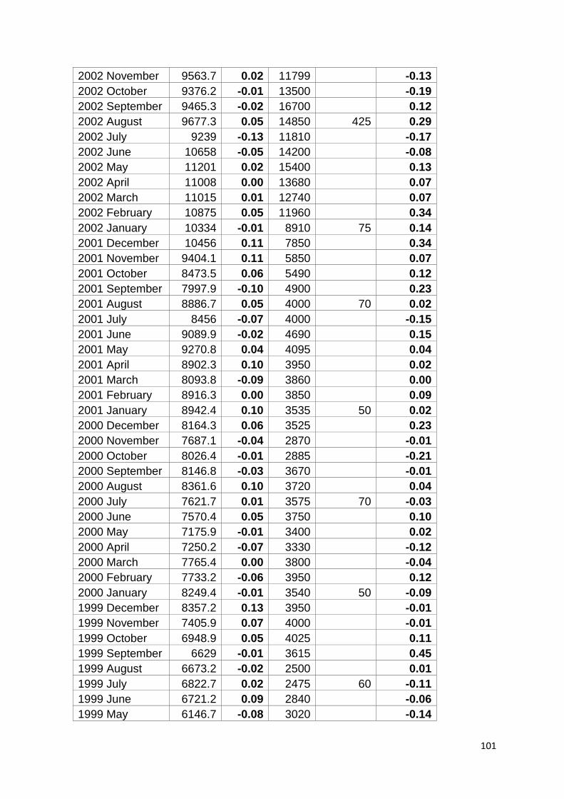
101

2002 November 9563.7 0.02 11799 -0.13

2002 October 9376.2 -0.01 13500 -0.19

2002 September 9465.3 -0.02 16700 0.12

2002 August 9677.3 0.05 14850 425 0.29

2002 July 9239 -0.13 11810 -0.17

2002 June 10658 -0.05 14200 -0.08

2002 May 11201 0.02 15400 0.13

2002 April 11008 0.00 13680 0.07

2002 March 11015 0.01 12740 0.07

2002 February 10875 0.05 11960 0.34

2002 January 10334 -0.01 8910 75 0.14

2001 December 10456 0.11 7850 0.34

2001 November 9404.1 0.11 5850 0.07

2001 October 8473.5 0.06 5490 0.12

2001 September 7997.9 -0.10 4900 0.23

2001 August 8886.7 0.05 4000 70 0.02

2001 July 8456 -0.07 4000 -0.15

2001 June 9089.9 -0.02 4690 0.15

2001 May 9270.8 0.04 4095 0.04

2001 April 8902.3 0.10 3950 0.02

2001 March 8093.8 -0.09 3860 0.00

2001 February 8916.3 0.00 3850 0.09

2001 January 8942.4 0.10 3535 50 0.02

2000 December 8164.3 0.06 3525 0.23

2000 November 7687.1 -0.04 2870 -0.01

2000 October 8026.4 -0.01 2885 -0.21

2000 September 8146.8 -0.03 3670 -0.01

2000 August 8361.6 0.10 3720 0.04

2000 July 7621.7 0.01 3575 70 -0.03

2000 June 7570.4 0.05 3750 0.10

2000 May 7175.9 -0.01 3400 0.02

2000 April 7250.2 -0.07 3330 -0.12

2000 March 7765.4 0.00 3800 -0.04

2000 February 7733.2 -0.06 3950 0.12

2000 January 8249.4 -0.01 3540 50 -0.09

1999 December 8357.2 0.13 3950 -0.01

1999 November 7405.9 0.07 4000 -0.01

1999 October 6948.9 0.05 4025 0.11

1999 September 6629 -0.01 3615 0.45

1999 August 6673.2 -0.02 2500 0.01

1999 July 6822.7 0.02 2475 60 -0.11

1999 June 6721.2 0.09 2840 -0.06

1999 May 6146.7 -0.08 3020 -0.14

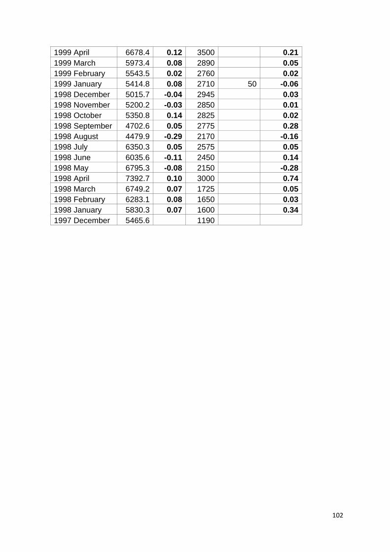
102

1999 April 6678.4 0.12 3500 0.21

1999 March 5973.4 0.08 2890 0.05

1999 February 5543.5 0.02 2760 0.02

1999 January 5414.8 0.08 2710 50 -0.06

1998 December 5015.7 -0.04 2945 0.03

1998 November 5200.2 -0.03 2850 0.01

1998 October 5350.8 0.14 2825 0.02

1998 September 4702.6 0.05 2775 0.28

1998 August 4479.9 -0.29 2170 -0.16

1998 July 6350.3 0.05 2575 0.05

1998 June 6035.6 -0.11 2450 0.14

1998 May 6795.3 -0.08 2150 -0.28

1998 April 7392.7 0.10 3000 0.74

1998 March 6749.2 0.07 1725 0.05

1998 February 6283.1 0.08 1650 0.03

1998 January 5830.3 0.07 1600 0.34

1997 December 5465.6 1190

103

7.7 Beta coefficients and discount rates for mining companies

7.7.1 Platinum mining companies

Period 1998-2002 1999-2003 2000-2004 2001-2005 2002-2006 2003-2007 2004-2008 2005-2009 2006-2010 2007-2011 2008-2012

Beta 0,96 1,57 1,83 1,83 1,66 1,71 1,68 1,65 1,61 1,54 1,49

Adjusted beta 0,99 1,40 1,58 1,58 1,47 1,50 1,48 1,46 1,43 1,39 1,35

Risk free rate (%) 6,40 6,40 6,40 6,40 6,40 6,40 6,40 6,40 6,40 6,40 6,40

ERP (%) 6,80 6,80 6,80 6,80 6,80 6,80 6,80 6,80 6,80 6,80 6,80

Cost of equity (%) 13,13 15,95 17,18 17,16 16,36 16,60 16,47 16,32 16,15 15,84 15,61

Beta 0,96 1,81 2,26 1,94 1,59 1,42 1,37 1,34 1,46 1,61 1,64

Adjusted beta 0,99 1,57 1,88 1,66 1,42 1,30 1,27 1,25 1,33 1,43 1,46

Risk free rate (%) 6,40 6,40 6,40 6,40 6,40 6,40 6,40 6,40 6,40 6,40 6,40

ERP (%) 6,80 6,80 6,80 6,80 6,80 6,80 6,80 6,80 6,80 6,80 6,80

Cost of equity (%) 13,16 17,08 19,15 17,66 16,04 15,26 15,03 14,91 15,44 16,16 16,30

Beta 0,87 1,41 1,50 1,58 1,39 1,40 1,64 1,48 1,65 1,67 1,66

Adjusted beta 0,93 1,30 1,36 1,41 1,28 1,29 1,45 1,35 1,46 1,47 1,47

Risk free rate (%) 6,40 6,40 6,40 6,40 6,40 6,40 6,40 6,40 6,40 6,40 6,40

ERP (%) 6,80 6,80 6,80 6,80 6,80 6,80 6,80 6,80 6,80 6,80 6,80

Cost of equity (%) 12,74 15,22 15,64 16,00 15,12 15,19 16,27 15,57 16,33 16,43 16,39

Platinum mining companies

Anglo American Platinum

Impala Platinum

Lonmin

104

7.7.2 Gold mining companies

Period 1998-2002 1999-2003 2000-2004 2001-2005 2002-2006 2003-2007 2004-2008 2005-2009 2006-2010 2007-2011 2008-2012

AngloGold Ashanti

Beta 0,73 0,73 0,90 0,99 1,08 1,19 0,88 0,81 0,50 0,42 0,33

Adjusted beta 0,84 0,83 0,95 1,02 1,08 1,15 0,94 0,89 0,68 0,63 0,57

Risk free rate (%) 6,40 6,40 6,40 6,40 6,40 6,40 6,40 6,40 6,40 6,40 6,40

ERP (%) 6,80 6,80 6,80 6,80 6,80 6,80 6,80 6,80 6,80 6,80 6,80

Cost of equity (%) 12,10 12,08 12,89 13,31 13,72 14,22 12,79 12,47 11,04 10,67 10,27

Gold Fields

Beta 0,66 0,78 0,95 1,12 1,41 0,00 0,84 0,64 0,30 0,21 0,11

Adjusted beta 0,79 0,87 0,99 1,10 1,30 0,34 0,91 0,78 0,54 0,49 0,42

Risk free rate (%) 6,40 6,40 6,40 6,40 6,40 6,40 6,40 6,40 6,40 6,40 6,40

ERP (%) 6,80 6,80 6,80 6,80 6,80 6,80 6,80 6,80 6,80 6,80 6,80

Cost of equity (%) 11,76 12,31 13,13 13,88 15,22 8,73 12,59 11,69 10,10 9,71 9,23

Harmony

Beta 0,81 0,91 1,17 1,40 2,04 2,29 1,36 0,88 0,37 0,15 0,06

Adjusted beta 0,89 0,96 1,13 1,29 1,72 1,89 1,27 0,94 0,60 0,44 0,38

Risk free rate (%) 6,40 6,40 6,40 6,40 6,40 6,40 6,40 6,40 6,40 6,40 6,40

ERP (%) 6,80 6,80 6,80 6,80 6,80 6,80 6,80 6,80 6,80 6,80 6,80

Cost of equity (%) 12,44 12,93 14,12 15,20 18,13 19,28 15,02 12,77 10,45 9,42 9,01

Gold mining companies

105

7.8 Summary of the descriptive statistics for mining companies


Measure Mean Standard Error Median Standard Deviation Sample Variance Kurtosis Skewness Range Minimum Maximum Sum Count



Equity component of WACC 12,43% 1,38% 12,53% 4,59% 0,002 3,304 1,484 16,67% 7,11% 23,78% 136,78% 11

CAPM 16,07% 0,33% 16,32% 1,09% 0,000 5,845 -2,119 4,05% 13,13% 17,18% 176,77% 11

Gordon's Wealth Growth Model13,78% 1,01% 13,01% 3,36% 0,001 -0,040 0,786 11,01% 9,62% 20,63% 151,61% 11

Impala Platinum

Equity component of WACC 13,96% 1,62% 13,55% 5,36% 0,003 -1,455 0,284 14,37% 7,60% 21,97% 153,56% 11

CAPM 16,02% 0,48% 16,04% 1,58% 0,000 0,952 0,313 6,00% 13,16% 19,15% 176,18% 11


Lonmin


CAPM 15,54% 0,32% 15,64% 1,06% 0,000 5,164 -2,047 3,69% 12,74% 16,43% 170,90% 11


106


Measure Mean Standard Error Median Standard Deviation Sample Variance Kurtosis Skewness Range Minimum Maximum Sum Count


AngloGold Ashanti

Equity component of WACC 10,40% 0,88% 11,37% 2,93% 0,001 -0,700 -0,558 8,80% 5,63% 14,43% 114,41% 11

CAPM 12,32% 0,38% 12,47% 1,26% 0,000 -0,797 -0,279 3,95% 10,27% 14,22% 135,56% 11


Gold Fields


CAPM 11,67% 0,62% 11,76% 2,04% 0,000 -0,816 0,123 6,49% 8,73% 15,22% 128,35% 11

Gordon's Wealth Growth Model10,62% 1,11% 11,28% 3,68% 0,001 8,245 -2,707 13,45% 0,11% 13,56% 116,81% 11

Harmony

Equity component of WACC 11,72% 1,36% 12,48% 4,52% 0,002 -1,331 -0,475 12,85% 4,47% 17,32% 128,96% 11

CAPM 13,52% 0,99% 12,93% 3,29% 0,001 -0,507 0,357 10,27% 9,01% 19,28% 148,77% 11

Gordon's Wealth Growth Model10,97% 0,63% 10,28% 2,08% 0,000 1,957 1,808 5,89% 9,62% 15,51% 120,67% 11

107

7.9 Input data of box and whisker plot for mining companies


Period 2002 2003 2004 2005 2006 2007 2008 2009 2010 2011 2012 Minimum Quartile 1 Median Quartile 3 Maximum Interquartile Range



Equity component of WACC 0,087 0,071 0,079 0,125 0,110 0,128 0,150 0,136 0,238 0,143 0,101 0,071 0,094 0,125 0,140 0,238 0,046

Difference N/A N/A N/A N/A N/A N/A N/A N/A N/A N/A N/A 0,071 0,023 0,031 0,014 0,098 N/A

CAPM 0,131 0,160 0,172 0,172 0,164 0,166 0,165 0,163 0,162 0,158 0,156 0,131 0,159 0,163 0,165 0,172 0,006


Gordon's Wealth Growth

Model 0,173 0,164 0,130 0,114 0,111 0,154 0,206 0,145 0,096 0,110 0,113 0,096 0,112 0,130 0,159 0,206 0,046


Impala Platinum



CAPM 0,132 0,171 0,192 0,177 0,160 0,153 0,150 0,149 0,154 0,162 0,163 0,132 0,151 0,160 0,167 0,192 0,015

Difference N/A N/A N/A N/A N/A N/A N/A N/A N/A N/A N/A 0,087 0,132 0,020 0,009 0,006 0,025


Model 0,173 0,166 0,157 0,121 0,113 0,115 0,175 0,176 0,111 0,122 0,133 0,111 0,118 0,133 0,169 0,176 0,052


Lonmin



CAPM 0,127 0,152 0,156 0,160 0,151 0,152 0,163 0,156 0,163 0,164 0,164 0,127 0,152 0,156 0,163 0,164 0,011



Model 0,163 0,152 0,152 0,125 0,109 0,115 0,163 0,118 0,096 0,105 0,130 0,096 0,112 0,125 0,152 0,163 0,040


108


Period 2002 2003 2004 2005 2006 2007 2008 2009 2010 2011 2012 Minimum Quartile 1 Median Quartile 3 Maximum Interquartile Range


AngloGold Ashanti



CAPM 0,121 0,121 0,129 0,133 0,137 0,142 0,128 0,125 0,110 0,107 0,103 0,103 0,116 0,125 0,131 0,142 0,015



Model 0,130 0,143 0,135 0,108 0,104 0,113 0,102 0,100 0,101 0,101 0,112 0,100 0,102 0,108 0,122 0,143 0,020


Gold Fields



CAPM 0,118 0,123 0,131 0,139 0,152 0,087 0,126 0,117 0,101 0,097 0,092 0,087 0,099 0,118 0,129 0,152 0,030



Model 0,109 0,132 0,136 0,104 0,102 0,113 0,118 0,117 0,106 0,109 0,131 0,102 0,107 0,113 0,125 0,136 0,017


Harmony



CAPM 0,124 0,129 0,141 0,152 0,181 0,193 0,150 0,128 0,105 0,094 0,090 0,090 0,114 0,129 0,151 0,193 0,037



Model 0,105 0,147 0,155 0,105 0,096 0,096 0,096 0,096 0,103 0,102 0,105 0,096 0,096 0,103 0,105 0,155 0,009


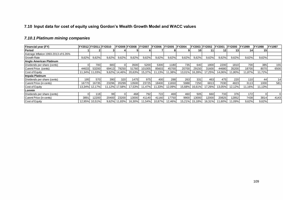
109

7.10 Input data for cost of equity using Gordon’s Wealth Growth Model and WACC values


Financial year (FY) FY2012 FY2011 FY2010 FY2009 FY2008 FY2007 FY2006 FY2005 FY2004 FY2003 FY2002 FY2001 FY2000 FY1999 FY1998 FY1997

Period 1 2 3 4 5 6 7 8 9 10 11 12 13 14 15

Average Inflation 1993-2013 of 6.26%

Growth Rate 9,62% 9,62% 9,62% 9,62% 9,62% 9,62% 9,62% 9,62% 9,62% 9,62% 9,62% 9,62% 9,62% 9,62% 9,62%

Dividends per share (cents) 0 700 683 0 3500 5200 5300 1180 735 640 1800 2200 1810 700 385 155

Curent Price (cents) 44633 53200 69413 79250 51760 101005 85603 45700 20700 29150 31600 44680 35200 18700 8070 6500

Cost of Equity 11,34% 11,03% 9,62% 14,46% 20,63% 15,37% 11,13% 11,38% 13,01% 16,39% 17,25% 14,06% 11,80% 11,87% 11,72%


Curent Price (in cents) 16770 16735 23296 20299 13500 23725 18400 11650 5988 7250 6813 7030 4823 3113 1000 581

Cost of Equity 13,34% 12,17% 11,12% 17,58% 17,53% 11,47% 11,33% 12,09% 15,68% 16,61% 17,26% 13,05% 12,12% 11,16% 11,13%



Cost of Equity 12,95% 10,51% 9,62% 11,83% 16,30% 11,54% 10,87% 12,46% 15,21% 15,18% 16,31% 11,60% 11,09% 9,62% 9,62%

Impala Platinum


Lonmin

110


Financial year (FY) FY2012 FY2011 FY2010 FY2009 FY2008 FY2007 FY2006 FY2005 FY2004 FY2003 FY2002 FY2001 FY2000 FY1999 FY1998 FY1997

Period 1 2 3 4 5 6 7 8 9 10 11 12 13 14 15

Average Inflation 1993-2013 of 6.26%

Growth Rate 9,62% 9,62% 9,62% 9,62% 9,62% 9,62% 9,62% 9,62% 9,62% 9,62% 9,62% 9,62% 9,62% 9,62% 9,62%



Cost of Equity 11,21% 10,08% 10,05% 9,98% 10,24% 11,30% 10,39% 10,84% 13,53% 14,33% 13,01% 13,25% 19,54% 14,98% 17,41%


Curent Price (in cents) 10375 12460 12060 9798 9190 9900 13275 11180 6950 9550 11990 5750 2570 2975 2350

Cost of Equity 13,10% 10,85% 10,62% 11,69% 11,82% 11,28% 10,20% 10,40% 13,56% 13,18% 10,94% 10,00% 13,03% 12,93% 16,61%


Curent Price (cents) 7400 9500 8300 7579 9770 7046 11120 8490 5120 10850 14700 7850 3525 3950 2945 1190

Cost of Equity 10,51% 10,19% 10,28% 9,62% 9,62% 9,62% 9,62% 10,52% 15,51% 14,67% 10,51% 11,29% 13,04% 9,62% 9,62%

AngloGold Ashanti

Gold Fields

Harmony

comparison of capital asset pricing model and …

Documents