comparison of benthic invertebrate community structure and … · 2017-05-31 · comparison of...
TRANSCRIPT

COMPARISON OF BENTHIC INVERTEBRATE COMMUNITY STRUCTURE AND
DIET COMPOSITION OF STEELHEAD (ONCORHYNCHUS MYKISS) IN DRY
CREEK, CALIFORNIA
By
Andrea Sue Dockham
A Thesis Presented to
The Faculty of Humboldt State University
In Partial Fulfillment of the Requirements for the Degree
Master of Science in Natural Resources: Fisheries
Committee Membership
Dr. Margaret Wilzbach, Committee Chair
Dr. Darren Ward, Committee Member
Dr. Gregg Horton, Committee Member
Dr. Alison O’Dowd, Committee Member
Dr. Alison O’Dowd, Graduate Coordinator
May 2016

ii
ABSTRACT
COMPARISON OF BENTHIC INVERTEBRATE COMMUNITY STRUCTURE AND
DIET COMPOSITION OF STEELHEAD TROUT (ONCORHYNCHUS MYKISS) IN
DRY CREEK, CALIFORNIA
Andrea Sue Dockham
Morphological changes in the Dry Creek (Sonoma County, California) associated
with Warm Spring Dam, have reduced habitat availability for rearing fish, and potentially
altered the community structure of benthic invertebrates that form the prey-base for
juvenile salmonids. I described and compared the structure of benthic invertebrate
assemblages and the diets of juvenile steelhead among four stream reaches of Dry Creek
downstream of Warm Springs Dam. I hypothesized that if prey availability contributes to
factors restricting the success of juvenile salmonids in mainstem Dry Creek, then diet
composition should parallel observed differences in reach-specific relative condition and
length of juvenile salmonids. Benthic invertebrate assemblages in Dry Creek displayed a
longitudinal trend from Warm Springs Dam to the confluence with the Russian River;
however, steelhead diet composition did not correspond with reach-specific benthic
invertebrate assemblages as expected. Drift-foraging is likely an important feeding
strategy for steelhead in mainstem Dry Creek. Steelhead condition and body length
corresponded with reach-specific differences in steelhead diet composition. However,
reach-specific differences in energetic cost associated with longitudinal differences in
water temperature (water temperature was positively correlated with distance from the

iii
dam) may be a greater contributor to differences in steelhead size. The relatively high
steelhead summer growth rates, in comparison with similar studies, may result from
artificially-sustained summer flows in mainstem Dry Creek. Year-round flows in
mainstem Dry Creek maintain stream connectivity during a period when non-regulated
streams in Mediterranean climates typically become disconnected, therefore increasing
food availability and foraging opportunities.

iv
ACKNOWLEDGEMENTS
I would like to thank Sonoma County Water Agency for providing funding for
this project. I would also like to express my extreme gratitude to the many people who
have provided me support and guidance during this process. Without them this would
not have been possible.
I would like to thank my advisor Margaret Wilzbach for her immense knowledge
of fisheries biology and aquatic invertebrates. I am very grateful for the many hours she
spent proving guidance and advice along the way, and all of her support for my career
outside of the graduate program.
I would like to thank Gregg Horton for his support while working at Sonoma
County Water Agency, even before starting the graduate program. I am thankful he was
able to be on my committee and provide me his knowledge of fisheries and the Dry Creek
watershed.
I would like to thank Alison O’Dowd for providing invaluable feedback and
guidance and asking me the hard questions that helped me see new aspects of the project.
I would like to thank Darren Ward for his knowledge of Pacific salmonid
bioenergetics and the feedback he provided on project design and thesis writing.
I would like to thank David Manning for providing me this opportunity in the first
place and always acknowledging the importance of studying aquatic invertebrates in the
fisheries field.

v
I would like to thank Michael Camman for providing his knowledge of
multivariate data analysis and the many hours he spent helping me.
I would like to thank Nicholas Som for providing his time and statistical support.
And finally, I would like to thank all of the many technicians at the Sonoma
County Water Agency for all of the hard work they provided for this project. I cannot
express how valuable all of their help was during fieldwork, sample sorting and data
entry. Thanks for being so awesome to work with.

vi
TABLE OF CONTENTS
ABSTRACT ........................................................................................................................ ii
ACKNOWLEDGEMENTS ............................................................................................... iv
LIST OF TABLES ............................................................................................................ vii
LIST OF FIGURES ........................................................................................................... ix
LIST OF APPENDICES .................................................................................................... xi
INTRODUCTION .............................................................................................................. 1
Study Site ........................................................................................................................ 7
MATERIALS AND METHODS ...................................................................................... 11
Data Analysis ................................................................................................................ 16
RESULTS ......................................................................................................................... 21
Benthic Macroinvertebrate Assemblages ..................................................................... 21
Steelhead Diet Composition ......................................................................................... 32
Steelhead Size and Prey Availability ............................................................................ 39
DISCUSSION ................................................................................................................... 41
Benthic Macroinvertebrate Assemblages ..................................................................... 41
Steelhead Diet Composition ......................................................................................... 44
Steelhead Size and Prey Availability ............................................................................ 45
RECOMMENDATIONS FOR FURTHER STUDY........................................................ 49
LITERATURE CITED ..................................................................................................... 50
Appendix A ....................................................................................................................... 58
Appendix B ....................................................................................................................... 64
Appendix C ....................................................................................................................... 66

vii
LIST OF TABLES
Table 1. Reach boundaries and predominant sediment supply in mainstem Dry Creek
downstream of Warm Springs Dam. ................................................................................. 11
Table 2. Major analytical questions and the analysis used. .............................................. 20
Table 3. Relative numerical abundance of the ten most abundant invertebrate taxa found
in benthic invertebrate kick net samples in spring and fall 2013 in Dry Creek. Relative
abundances for each taxon were calculated from combined count data from 36 samples
for each season. ................................................................................................................. 22
Table 4. Results of permutational MANOVA to determine effect of categorical data on
grouping of benthic invertebrate community structure in Dry Creek. .............................. 23
Table 5. Results from non-metric multidimensional scaling (NMDS) regression and
ANOVA on community metrics and environmental variables between seasons. All
samples were collected in spring and fall 2013 in Dry Creek, Sonoma County, California.
Data were summarized from 36 samples for each season. ............................................... 25
Table 6. Results of permutational MANOVA to determine effect of categorical data on
grouping of benthic invertebrate community structure in Dry Creek in spring and fall... 27
Table 7. Results from non-metric multidimensional scaling (NMDS) regression analysis
and ANOVA of community metrics and environmental variables among reaches. Data
were summarized from 36 samples, collected in spring 2013, with each sample
representing a composited collection of 3 samples along a channel cross-section.
Reaches listed from downstream to upstream. ................................................................. 30
Table 8. Results from non-metric multidimensional scaling (NMDS) regression analysis
and ANOVA of community metrics and environmental variables among reaches. Data
were summarized from 36 samples, collected in fall 2013 with each sample representing
a composited collection of 3 samples along a channel cross-section. Reaches listed from
downstream to upstream. .................................................................................................. 31
Table 9. ANOVA analysis of the effect of reach on prey biomass, prey abundance, and
percent of the diet composed of the three most abundant taxa in diet samples of young of
year steelhead. Up to 20 diet samples were collected per reach in fall 2013 from four
reaches in Dry Creek. The contiguous reaches extended from just downstream of Warm
Springs Dam (reach 4) to the confluence of the creek with the Russian River (reach 1). 33
Table 10. Relative numerical abundance of the ten most abundant taxa found in steelhead
(Oncorhynchus mykiss) diet samples collected in fall 2013, for each reach in Dry Creek,

viii
Sonoma County, California. Reaches are shown in order from downstream to upstream.
........................................................................................................................................... 36
Table 11. Results of Bray-Curtis dissimilarity index (0 = totally similar; 1 = totally
dissimilar) comparing steelhead diet samples to benthic invertebrate samples by reach in
Dry Creek. All samples were collected in the fall of 2013. Reaches are shown in order
from downstream to upstream. ......................................................................................... 37
Table 12. Summary of relative condition of fish in fall 2013 from four contiguous reaches
in Dry Creek, and results of Tukey’s HSD post hoc comparison. Reaches extended from
just downstream of Warm Springs Dam (reach 1) to the confluence of the Dry Creek with
the Russian River (reach 4). .............................................................................................. 40
Table 13. Summary of length (mm) of fish in fall 2013 from four contiguous reaches in
Dry Creek, and results of Tukey’s HSD post hoc comparison. Reaches extended from
just downstream of Warm Springs Dam (reach 1) to the confluence of Dry Creek with the
Russian River (reach 4). .................................................................................................... 40

ix
LIST OF FIGURES
Figure 1. Average daily streamflow in Dry Creek, California, pre and post construction of
Warm Springs Dam in 1984. Flow data were obtained from the USGS gauging station
near Geyserville, California (USGS 11465200). ................................................................ 3
Figure 2. Estimated growth rates of juvenile steelhead from mainstem Dry Creek, 2010
through 2013. Estimates are from individual growth rates calculated as the change in
fork length (mm) per day of PIT-tagged fish between initial tagging in July and recapture
in late September/ early October. Used with permission from Manning and Martini-
Lamb (2014)........................................................................................................................ 4
Figure 3. Map of lower Dry Creek watershed in Sonoma County California, including
study reach delineations and location of riffles sampled within each reach. ...................... 8
Figure 4. Diagram of benthic invertebrate subsampling in each riffle. Each subsample
was combined to form one sample. Three samples were taken per riffle. ....................... 12
Figure 5. NMDS plot of spring and fall 2013 benthic invertebrate samples coded by study
reach in Dry Creek (1-4). Continuous variable vectors show correlations of community
metrics and habitat variables with benthic samples. Rich= taxonomic richness, div=
Brillouin’s diversity index, even= Camargo’s evenness, dom3= proportion of sample
made up of the three most dominant taxa and H20temp= water temperature (± 0.1
degrees C) Do2= dissolved oxygen (± 0.01 mg/L), stcover= percent stream cover. Taxa
codes are listed in Appendix C. ........................................................................................ 24
Figure 6. NMDS plot of spring 2013 benthic invertebrate samples coded by study reach
in Dry Creek. Continuous variable vectors show correlations of community metrics and
habitat variables with benthic samples. Rich= taxonomic richness, div= Brillouin’s
diversity index, even= Camargo’s evenness, dom3= proportion of sample made up of the
three most dominant taxa and H20temp= water temperature (± 0.1 degrees C) Do2=
dissolved oxygen (± 0.01 mg/L), stcover= percent stream cover. Taxa codes are listed in
Appendix C. ...................................................................................................................... 28
Figure 7. NMDS plot of fall 2013 benthic invertebrate samples coded by study reach in
Dry Creek. Continuous variable vectors show correlations of community metrics and
habitat variables with benthic samples. Rich= taxonomic richness, div= Brillouin’s
diversity index, even= Camargo’s evenness, dom3= proportion of sample made up of the
three most dominant taxa and H20temp= water temperature (± 0.1 degrees C) Do2=
dissolved oxygen (± 0.01 mg/L), stcover= percent stream cover. Taxa codes are listed in
Appendix C. ...................................................................................................................... 29

x
Figure 8. NMDS plot of fall 2013 steelhead (Oncorhynchus mykiss) diet samples coded
by study reach in Dry Creek. Taxa codes are listed in Appendix C. ............................... 35
Figure 9. Comparisons of relative abundance of the 10 most abundant taxa found in
benthic invertebrate samples and steelhead diet samples for each reach in Dry Creek.
Samples were collected in fall 2013. Reaches are shown in order from downstream to
upstream. Taxa codes are listed in Appendix C. .............................................................. 38
xi
LIST OF APPENDICES
Appendix A. Length-weight regression equations for aquatic life stages of invertebrates
based on body length. The only exception was in the case of Dixa (Diptera: Dixidae),
which used head capsule width (HW). Equations are in the form of DM=a (Lb) unless
otherwise noted. DM = dry mass, L= body length and a and b are fitted coefficients. For
regression equations that calculated ash-free dry mass (AFDM) instead of DM, AFDM
was converted to DM using the equation: M = AFDM (100100-%ash). If coefficients
from a different taxon were used to calculate DM, taxon is indicated in parenthesis. ..... 58
Appendix B. Length-weight regression equations for adult life stages of invertebrates
based on body length. The only exception was in the case of Armadillidium (Isopoda:
Armadillidae), which used head capsule width (HW). Equations are in the form of
DM=a(Lb) unless otherwise noted. DM = dry mass, L= body length and a and b are fitted
coefficients. If coefficients from a different taxon were used to calculate DM, taxon are
indicated in parenthesis. .................................................................................................... 64
Appendix C. Invertebrate taxa identified from benthic samples and diet samples of
juvenile steelhead in Dry Creek, Sonoma County, California spring and fall 2013 and
their corresponding taxa codes. All taxa were collected in benthic samples and/or diet
samples. ............................................................................................................................. 66

1
INTRODUCTION
Dams can profoundly affect the morphology of a river and the organisms they
support. Downstream of an impoundment, the river setting is affected by changes in
flow, sediment supply, temperature, and water quality. Trapping of sediments in the
impoundment results in a loss of sediments downstream which can promote bank and
channel erosion, channel incision, and armoring of the streambed (e.g., Ward and
Stanford 1983, Ligon et al. 1995, Wang et al. 2011). Loss of flushing flows from
stabilized flow regimes can result in an aggraded streambed and reduced substrate
heterogeneity if fine sediments are present (Poff and Hart 2002). Biological responses
can include increased periphyton abundance immediately downstream of a dam as water
transparency increases (Stanford and Ward 1979), changes in species composition of
aquatic assemblages, reduction in taxonomic diversity, and restricted movement of
organisms as lateral and longitudinal connectivity of the river is severed (e.g., Bayley
1991; Boulton and Lloyd 1992; Freeman et al. 2001). However, if the reservoir release is
from bottom of the water supply pool, changes in the water temperature regime can
enhance opportunities for growth of juvenile salmon if previous temperatures were not
favorable (Brett 1952).
Prior to dam construction, Dry Creek, located in the Russian River drainage in
coastal northern California, was an intermittent stream running dry or nearly so in the
summer and fall with only a few disconnected pools. Winter storm discharges were up to
three orders of magnitude higher than summer flows (Figure 1) and summer water

2
temperatures typically exceeded 20o C from May through October (Inter-Fluve
2010). Dry Creek historically supported native populations of Sacramento Suckers
(Catostomus occidentalis), Sacramento Pikeminnow (Ptychocheilus grandis), and
California Roach (Hesperoleucus symmetricus), while salmonids were less common
(Hopkirk and Northen 1980). Since the completion of the Warm Springs Dam in 1984,
streamflows in Dry Creek have become perennial with much less seasonal variability in
flow. Year-round releases of cold water from Warm Springs Dam have enabled
mainstem Dry Creek to support populations of state and federally listed endangered and
threatened salmonids: Coho Salmon (Oncorhynchus kitsutch) (Central California Coast
ESU), steelhead (Oncorhynchus mykiss) (Central California Coast ESU), and Chinook
Salmon (Oncorhynchus tshawytscha) (California Coastal ESU). However, the dam has
affected sediment transport and altered riparian vegetation, resulting in a highly incised,
narrow channel that lacks natural sinuosity. High flows, coupled with extensive channel
incision and bank erosion, are believed to limit both the quantity and quality of winter
and summer rearing habitats in the creek for juvenile steelhead and Coho Salmon.

3
Figure 1. Average daily streamflow in Dry Creek, California, pre and post construction of Warm
Springs Dam in 1984. Flow data were obtained from the USGS gauging station near
Geyserville, California (USGS 11465200).

4
To increase summer rearing habitat and provide winter flow refugia for salmonids
in Dry Creek, the Sonoma County Water Agency is currently implementing habitat
enhancement projects to enhance more than 9.5 km of the 22 km downstream of Warm
Springs Dam. In the Russian River Biological Opinion Status and Data Report 2013-14
(Martini-Lamb and Manning 2014), validation-monitoring results from 2010 through
2013 showed that mean individual growth rates of juvenile salmonids were significantly
lower in the upper portion of Dry Creek downstream of the dam than in the middle or
lower portions of the creek (Figure 2). Differences in growth rates among river sections
may reflect a diminished effect of the dam on channel morphology and riverine ecology
with increased distance downstream from the dam.
Figure 2. Estimated growth rates of juvenile steelhead from mainstem Dry Creek, 2010 through
2013. Estimates are from individual growth rates calculated as the change in fork length
(mm) per day of PIT-tagged fish between initial tagging in July and recapture in late
September/ early October. Used with permission from Manning and Martini-Lamb
(2014).

5
Most programs aimed at restoring habitat to benefit anadromous salmonids have
focused on physical habitat elements (e.g. creating or increasing slow water habitats to
provide refugia during high flows, enhancing channel complexity), but have failed to
adequately consider the riverine ecology and associated food webs, which in some cases,
may be even more limiting to salmonid production than abiotic factors such as physical
habitat and water quality. Population density of salmonids is mediated by habitat quality,
but salmonid growth can be low when fish densities are high even in high quality habitat
(Grant and Imre 2005). Salmonid production, which is often measured as the product of
fish biomass (density) and growth (%/day), is often more strongly affected by high
growth than by population density (Bisson and Bilby 1998). High growth rates require
abundant food resources, even when physical habitat and water quality are favorable (Dill
et al. 1981). Somatic growth rates are a function of food availability, metabolic costs of
obtaining and processing food, and density-dependent biotic interactions including
predation and competition (Fausch 1984).
Dam-related longitudinal effects on aquatic invertebrate assemblages are well
described (eg. Ward and Stanford 1983, Stanford and Ward 2001, Power et al. 1996) and
have been found to affect the food web structure and food available to support salmonid
production. This may be the case in Dry Creek as well. Other studies have observed that
taxonomic richness is generally lower just downstream of a dam as compared to reaches
further downstream (e.g. Growns et al. 2009, Marchant and Hehir 2002, Hynes 1970,
Petts and Greenwood 1985, Vinson 2001). Reasons include reduced water quality due to
increase in concentration of nutrients and metals in tailwater (Growns et al. 2009), lack of

6
colonization from drift (Marchant and Hehir 2002), loss of habitat heterogeneity (Hynes
1970; Petts and Greenwood 1985), and decreased temperature variability (Vinson 2001).
If decreases in abundance and diversity of benthic invertebrate assemblages occur in
reaches just downstream of a dam, recovery to reference conditions may not occur until a
considerable distance downstream of the impoundment (Growns et al. 2009). I predict
that invertebrate assemblages in mainstem Dry Creek are decreased in abundance and
diversity relative to reference conditions in reaches closest to Warm Springs Dam, and
the resulting decrease in food availability is causing the observed lower growth rates of
steelhead in upper reaches of Dry Creek that are nearer the dam.
This study characterizes and compares the structure of benthic invertebrate
assemblages in reaches extending from Warm Springs Dam to the creek’s confluence
with the mainstem Russian River, and assesses the relationships between the structure of
reach-specific benthic invertebrate assemblages with diet composition, relative condition,
and body length of juvenile steelhead. If prey availability is contributing to factors
limiting production of juvenile steelhead in Dry Creek, my expectation is that reach-
specific differences in prey availability should correspond with observed differences in
reach-specific relative condition and length of juvenile salmonids.
Specific objectives are to:
1) Characterize and compare the structure of benthic invertebrate communities in
contiguous reaches of Dry Creek.
2) Characterize and compare reach-specific diet composition by juvenile (>60 mm FL)
steelhead in Dry Creek.

7
3) Evaluate reach-specific correspondence of diet composition with condition and length
of juvenile steelhead trout.
By examining whether or not food resources are a limiting factor to size and
condition of steelhead in mainstem Dry Creek, managers can improve restoration efforts
that aim to provide productive benthic macroinvertebrate habitat and create optimal
foraging opportunities for rearing juvenile salmonids.
Study Site
Dry Creek is a fourth-order tributary to the Russian River in northern California
(Figure 3). The Dry Creek watershed, including the area above Warm Springs Dam,
drains 349.2 km2 of rugged terrain in the southwestern portion of the Russian River
Basin. Crane Creek, Grape Creek, Mill Creek, and Peña Creek are its main
tributaries. The climate is Mediterranean with warm dry summers and cool wet winters
(Gasith and Resh 1999). Average monthly air temperature ranges from 8.3o C in the
winter to 21.4o C in the summer and annual precipitation averages 110 cm. Most of the
land in the catchment is privately owned and used for agriculture, with wine grapes being
the primary crop (Inter-Fluve 2010).

8
Figure 3. Map of lower Dry Creek watershed in Sonoma County California, including study reach
delineations and location of riffles sampled within each reach.

Warm Springs Dam is located 22.4 kilometers upstream of the confluence of Dry
Creek with the Russian River, and entirely blocks anadromous fish passage. The Dry
Creek channel downstream of the dam is primarily composed of pool-riffle and plane-bed
morphology with an average channel gradient of 0.18% (Inter-Fluve 2010). The alluvial
bed consists mostly of gravel but ranges from sand to bedrock (Inter-Fluve 2011). Water
temperatures remain fairly constant throughout the year, with an average of 13o C near
the dam and gradually rising to 16o C at near the confluence with the Russian River.
The current hydrologic regime of Dry Creek downstream of Warm Springs Dam,
provides more moderate winter floods and higher sustained summer flows than do other
Russian River tributaries (Figure 1). Daily releases from Warm Springs Dam remain
very consistent throughout the day and seasonal releases are influenced by municipal
water demands, typically in the late spring through fall, or rain events in the winter. In
the summer and early fall when municipal water demands are high, daily releases average
1.16 m3.s-1 (DWR 2015). Median annual peak flows from 1984 through 2008 were
112.13 m3.s-1 and occurred in the winter or early spring (Interfluve 2010). In 2013 when
this study was conducted, peak flow reached 88 m3.s-1; based on a 29-year period of
record (1984 – 2013), the recurrence interval for flows of this magnitude is estimated to
be 1.6 yr. Peak flow data were obtained from the USGS gauging station near
Geyserville, California (USGS 11465200).
The riparian zone of Dry Creek has encroached on the active channel, with
extensive vegetation on gravel bars that were active prior to the completion of the dam
but are largely inactive today because of the heavily vegetated riparian corridor. In some

10
sections, the riparian canopy has completely enclosed the active stream channel
(Interfluve 2010). Dominant over story species include: red willow (Salix leavigata), box
elder (Acer negundo), and white alder (Alnus rhombifolia) with an occasional cottonwood
(Populus fremontii) and California bay (Umbellularia californica). The understory is
dominated by Himalayan blackberry (Rubus discolor), California blackberry (Rubus
ursinus var. ursinus), escaped grape (Vitis vinifera), and mugwort (Artemisia
douglasiana) (Cuneo 2011).
The fish assemblage of Dry Creek is primarily composed of native species
(Sonoma County Water Agency unpublished data). In addition to steelhead and Coho
Salmon and Chinook Salmon, other native species include the federally threatened
(Central California Coast ESU) Chinook Salmon (Oncorhynchus tshawytscha),
California Roach, Hardhead (Mylopharodon conocephalus), Pacific Lamprey
(Entosphenus tridentatus), Prickly Sculpin (Cottus asper), Sacramento Pikeminnow,
Sacramento Sucker, and Russian River Tule Perch (Hysterocarpus traskii pomo). Non-
native species include: Bluegill (Lepomis macrochirus), Green Sunfish (Lepomis
cyanellus), Largemouth Bass (Micropterus salmoides), and Smallmouth Bass
(Micropterus dolomieu).

11
MATERIALS AND METHODS
For purposes of validation monitoring, the Sonoma County Water Agency
originally divided mainstem Dry Creek into three reaches based on geomorphic
differences in sediment source and supply (Table 1). For this study, the original reach
two was further divided into two reaches to create four reaches that were similar in
length. Reach one began at the confluence of Dry Creek with mainstem Russian River
and reach four ended at Warm Springs Dam (Table 1).
Table 1. Reach boundaries and predominant sediment supply in mainstem Dry Creek downstream
of Warm Springs Dam.
Study
reach Rkm Upstream landmark Primary sediment source
1
0-4.8
Fault lineament
Backwater from confluence
with the Russian River.
2
4.8-10
Bedrock outcrop
Tributaries
3
10-17.7
Pena Creek
Tributaries
4
17.7-22.4
Warm Springs Dam outlet
Impounded (no supply)
Within each of the four reaches, benthic invertebrate samples were collected from
three randomly selected riffles per reach, and three samples were collected within each
riffle (n = 36 samples per sampling event) (Figure 3, Figure 4). Collections were made
during late spring and early fall 2013 (total n = 72). Spring sampling locations within
each riffle were initially chosen using systematic random sampling (Cochran 1977); fall
samples were collected in the same locations as the spring samples. Geographic
coordinates of sampling locations were recorded using a GPS unit.

12
Figure 4. Diagram of benthic invertebrate subsampling in each riffle. Each subsample was
combined to form one sample. Three samples were taken per riffle.

13
In each of the three sample locations within a riffle, three subsamples were taken
along the channel cross-section to capture the range of habitat variability present (Figure
4). Due to safety concerns deep, fast moving habitat was excluded from sampling if it
was present in a cross-section. Otherwise, if stream conditions were generally uniform in
velocity, substrate, and water depth, samples were collected at three equidistant locations
along the cross-section. Samples were collected using a 500-μm mesh D-frame net. An
approximate area of 0.3 m2 of substrate immediately upstream of the net was agitated for
one minute and large rocks were scrubbed by hand in front of the net to remove attached
invertebrates. Subsamples were composited to create one sample, and samples were
preserved in 70% ethanol.
Habitat data were collected in each riffle in the spring and fall to characterize
variability within and between reaches, and to determine if dam-related effects on habitat
affected invertebrate assemblages among reaches. While all habitat variables were
chosen because they were hypothesized to be affected by Warms Springs Dam, percent
canopy cover was also chosen because of the potential effect of the amount of shading
and allocthonous input that a well-established riparian vegetation community (as is
characteristic of Dry Creek) can have on invertebrate assemblages (Vannote et al. 1980).
At each sample point within a riffle, velocity (± 0.01 cm· s-1) and depth (± 0.01 m) were
measured and substrate composition was visually estimated using the following
categories: fines (<2 mm), gravel (2-32 mm), cobble (32-256 mm), boulder (>256 mm)
and bedrock (solid). In each riffle, percent canopy cover, temperature (± 0.1 degrees C)

14
and dissolved oxygen (± 0.01 mg/L) were measured and percent canopy cover was
visually estimated. Dissolved oxygen was measured with a YSI ® Model 85.
In the laboratory, invertebrate taxa were identified, measured, and enumerated
based on a subsample of 300 individuals per composite sample. Subsampling was
conducted following the protocols of Barbour et al. (1999) using a numbered and gridded
tray and a random number table. Contents of the chosen square were placed into a petri
dish for inspection under a dissecting scope with adjustable magnification (up to 60x).
All individuals from the petri dish were sorted from debris and placed in a vial containing
70% ethanol. Contents of each petri dish were examined three times to ensure that all
invertebrates were removed. This process was repeated until 300 invertebrates were
picked from the sample. The remainder of the sample was archived in 70%
ethanol. Invertebrates from subsamples were sorted under a dissecting microscope and
identified to the lowest feasible taxonomic level using keys in Merritt et al. (2008) and
Smith (2001). Individuals within the class Insecta were identified to genus with some
exceptions. Chironomidae individuals were identified to family, except for individuals in
Tanypodinae individuals, which were identified to sub-family. Non-Insect fauna were
identified to order unless a higher level of taxonomic resolution was achievable. Lengths
of individuals were measured to the nearest millimeter from head to abdomen. Cerci
were not included in measurements.
Procedures for sampling and handling of fish were approved under Humboldt
State University IACUC Protocol 12/13.F79-A. For measurement of fish condition and
diet sampling, juvenile steelhead were collected in each reach over one week in fall 2013

15
using backpack electrofishers. Diet samples were collected one week after fall benthic
invertebrate samples were collected to allow fish to move back into sampling areas after
being disturbed during kick net sampling. Electrofishing sections were approximately
46m long and the number of electrofishing sites varied among reaches based on
landowner access and whether conditions were suitable for safe sampling with a
backpack electrofisher sampling. Two passes were made in each section with the first
pass beginning at the downstream end of the section and ended at the upstream end. The
second pass began at the upstream end and ending at the downstream end. High flows
prevented the use of block nets. All fish captured in a given section were measured for
length (±1 mm) and weight (±0.1 g) and passive integrated transponders were applied to
individual steelhead ≥60 mm. Diet samples were collected from the first five steelhead
from each section until 20 samples per reach was obtained (n = 80). If a reach had more
than four sections, steelhead were selected for diet sampling from alternating sections to
ensure samples were uniformly distributed throughout the reach. Fish were released at
the location of capture (±46 m) following recovery from the anesthetic. Because of
federal endangered species act permit constraints, only diets of steelhead ≥60 mm were
sampled.
Fish selected for diet sampling were first anesthetized using a 40 mg.L-1 solution
of buffered MS222. Diet samples of juvenile steelhead were collected using a 7.6 L
garden sprayer with a narrow pipe attachment. The sprayer was filled with stream water
and filtered through a 500µm mesh sieve. The pipe attachment was inserted into the
mouth of a fish and a stream of water was applied using minimal water pressure until

16
foregut contents were flushed into a 500µm sieve. Samples were preserved in 70%
ethanol. Invertebrates from diet samples were identified, measured and enumerated as
described for benthic invertebrate samples. Subsampling was not conducted since the
total number of taxa per sample was small enough to allow for timely processing of gut
samples. Due to the deteriorated nature of gut contents, the level of taxonomic resolution
was coarser for diet samples than for benthic invertebrate samples, and length
measurements were sometimes estimated from body parts. Head capsules were counted
as individuals in the absence of an intact body. Winged adults that had an aquatic life
stage were considered to be aquatic taxa. Terrestrial organisms included all taxa that did
not have an aquatic life stage; these were lumped into a separate group.
Data Analysis
Questions asked and the analytical tools used to answer these are summarized in
Table 2. Benthic macroinvertebrate assemblages were described using community
metrics including Brillouin’s diversity index (Pielou 1967), Camargo’s evenness
(Camargo 1993), taxonomic richness, relative abundance and percentage of abundance
comprised by the three most dominant taxa (dom3) (Plafkin et al. 1989). While the
purpose of this study is to determine prey availability for steelhead in mainstem Dry
Creek, these metrics are used to describe the overall benthic community structure as a
baseline for comparison to steelhead diet compositions. Some of these metrics can be
used to complement one another. For examples, taxonomic richness determines the
number of taxa present in a community while the metrics of diversity (Brillouin’s

17
diversity and Camago’s evenness) can illustrate how well the taxa are represented within
the community.
Permutational MANOVA was used to test effects of categorical variables on
benthic community structure in mainstem Dry Creek (McArdle and Anderson
2001). Explanatory variables used to fit the model were season (spring, fall), reach (one -
four) and substrate size class (fines, gravel, cobble, boulder, bedrock). Since reach
delineation was based on differences in sediment source and supply, multi-response
permutation procedure (MRPP) using the Bray-Curtis dissimilarity index was used to
further test whether substrate size classes affected invertebrate assemblages with season
(Zimmerman et al. 1985) and a Kruskal-Wallis chi-squared was used to test whether
substrate size class significantly differed between reaches as assumed. MRPP is a non-
parametric multivariate test and provides the statistic A and a p-value. The statistic A is a
chance-corrected estimate of the proportion of the distances explained by group identity
(Oksanen et al. 2007).
Benthic invertebrate community structure was characterized using non-metric
multidimensional (NMDS) ordination plots using Bray-Curtis dissimilarity matrices.
NMDS is an ordination method that constructs a configuration of points in a specific
number of dimensions, based on ranked distances between samples (Minchin 1987).
Only taxa that were present in at least 20 percent of the samples were used for
calculations to avoid distortion by rare taxa (Austin and Greig-Smith 1968). Samples
were color-coded by reach, and plots to observe reach-specific groupings of samples
without separation by season were created along with plots of samples separated by fall

18
and spring. Covariate vectors were fitted to the benthic invertebrate sample data using
NMDS regression; these were overlaid on plots to observe relationship of continuous
environmental variables and community metrics with reach-specific grouping of samples.
ANOVA was used to test whether environmental variables and community metrics
differed between seasons and among reaches and results were compared to NMDS
regression results.
Differences in steelhead diet composition among reaches were visualized using an
NMDS plot with diet samples coded by reach. MRPP using the Bray-Curtis dissimilarity
index was used to test whether steelhead diet composition differed among reaches.
Bray-Curtis dissimilarity index was used to compare steelhead diet composition
data to fall benthic samples to evaluate the correspondence between reach-specific
benthic invertebrate assemblages and prey selection. I compared the relative numerical
abundance of the top 10 taxa for each reach in benthic invertebrate samples to the relative
numerical abundance of the top 10 taxa in the corresponding reaches in the diet samples
using pie charts.
ANOVA was used to determine if relative condition of fish and fork length (FL)
differed among reaches and if differences corresponded with reach-specific differences in
growth found in previous monitoring studies. Differences in length were analyzed in
addition to relative condition to account for any potential parr-smolt transformation effect
on relative condition of juvenile steelhead (Fessler and Wagner 1969). Relative
condition was calculated as 𝐾𝑛 = (𝑊/𝑊’), where W is the weight of the fish and W’ is
the length specific mean weight of a fish in the population being studied. W’ was

19
calculated as log(𝑊′) = 𝑎’ + 𝑏 × log(𝐿), where a’ is the intercept and b is the slope of
the length-weight regression (Murphy and Willis 1996). Based on length and weight data
of fish collected during fall electrofishing in Dry Creek (n=947), coefficient a’ was
estimated as -4.8414 and coefficient b was estimated as 2.99505. Lengths and weights of
fish were logarithmically transformed to account for allometric growth (Murphy and
Willis 1996).
Linear regression was used to evaluate reach-specific correspondence of diet
composition with condition of juvenile steelhead. Biomass and abundance were
calculated from the steelhead diet samples and used to represent diet composition in
linear regression analysis. Dom3 was chosen as well to examine whether or not diets,
which were dominated by a few taxa, had a positive or negative affect on condition and
size of fish. Effect of reach on diet metrics was evaluated using ANOVA. Biomass was
estimated using published invertebrate length-weight regressions (Appendix A, Appendix
B). Abundance was estimated as the total number of prey items in a sample.

20
Table 2. Major analytical questions and the analysis used.
Analytical Question Analysis Method
Benthic
Macroinvertebrate
Assemblages
What is the effect of season, reach,
and substrate size class on benthic
invertebrate assemblages?
Permutational
MANOVA
How similar were benthic samples in
composition (based on Bray-Curtis
dissimilarity matrices), overall and
separated by season?
NMDS plots
How does continuous environmental
variables and community metrics
correlate with reach-specific grouping
of samples?
NMDS regression
Were community metrics and habitat
variables different between reach and
season?
ANOVA, Kruskal-
Wallis test
Steelhead Diet
Composition
What is the effect of reach on diet
composition?
MRPP, NMDS plot
What is the effect of reach on diet
metrics (biomass, abundance, dom 3)?
ANOVA
What was the correspondence
between diet composition and benthic
invertebrate assemblages?
Bray-Curtis
dissimilarity index, Pie
charts comparing
relative abundance of
top 10 taxa.
Steelhead Size and
Prey Availability
What is the effect of reach on fish
condition and fish length?
ANOVA, Tukey’s
HSD
What is the effect of prey biomass,
prey abundance, and percent of total
prey composed of top 3 taxa on fish
condition and fish length?
Linear regression (not
performed because diet
metrics were not
significantly different
among reaches)
21
RESULTS
Benthic Macroinvertebrate Assemblages
A total of 71 taxa were identified from benthic invertebrate samples (Appendix
C). The majority of taxa identified belonged to the class Insecta, while a smaller number
of taxa were from non-insect arthropod groupings (i.e.,Crustacea, Acari), and phyla
including the segmented worms (Annelida), flatworms (Platyhelminths), and Mollusca.
The highest taxonomic richness observed within a riffle included 39 taxa and the lowest
was 21 taxa. Chironomidae (Diptera) was the most abundant taxa found during
sampling. In samples separated by season, Chironomidae, Baetis (Ephemeroptera:
Baetidae) and Optioservus (Coleoptera: Elmidae), were the three most abundant taxa in
spring samples, while Optioservus, Rhithrogena (Ephemeroptera: Heptageniidae), and
Chironomidae were the most abundant taxa in the fall (Table 3). Trichoptera had high
abundance in the spring; three taxa (Lepidostoma, (Trichoptera: Lepidostomatidae)
Hydropsyche (Trichoptera: Hydropsychidae) and Glossosoma (Trichoptera:
Glossosomatidae) made up 26% of the relative abundance found in spring samples (Table
3). Overall, fall had more taxa represented in the benthic samples (71) than the spring
samples (62).

22
Table 3. Relative numerical abundance of the ten most abundant invertebrate taxa found in
benthic invertebrate kick net samples in spring and fall 2013 in Dry Creek. Relative
abundances for each taxon were calculated from combined count data from 36 samples
for each season.
Taxa
Relative
Abundance
Spring
Chironomidae (Diptera) 0.25
Baetis (Ephemeroptera: Baetidae) 0.16
Optioservus (Coleoptera: Elmidae) 0.12
Lepidostoma (Trichoptera: Lepidostomatidae) 0.10
Hydropsyche (Trichoptera: Hydropsychidae) 0.07
Oligochaeta 0.06
Glossosoma (Trichoptera: Glossosomatidae) 0.06
Simulium (Diptera: Simuliidae) 0.04
Acari 0.04
Tanypodinae (Diptera: Chironomidae) 0.01
Fall
Optioservus 0.20
Rhithrogena (Ephemeroptera: Heptageniidae) 0.19
Chironomidae 0.12
Baetis 0.11
Isoperla (Plecoptera: Perlodidae) 0.06
Lepidostoma 0.04
Oligochaeta 0.03
Tricorythodes (Ephemeroptera: Leptohyphidae) 0.03
Hydropsyche 0.02
Acari 0.02

23
Benthic invertebrate assemblages in Dry Creek differed between seasons, and
among reaches and substrate type (Table 4). Seasonal differences in benthic invertebrate
assemblages were reflected in the NMDS plot (Figure 5). In addition, seasonal grouping
of samples were highly correlated with the community metrics of taxonomic richness and
diversity, as well as the environmental variables of dissolved oxygen concentration and
velocity (Figure 5). Of these significantly correlated variables, dissolved oxygen,
velocity, taxonomic richness and diversity differed significantly between spring and fall
(Table 5). Taxonomic richness, diversity, and dissolved oxygen concentrations were
greater in the fall; mean velocities were higher in the spring (Table 5).
Table 4. Results of permutational MANOVA to determine effect of categorical data on grouping
of benthic invertebrate community structure in Dry Creek.
Variable D.F. SS MS F p
Season 1 2.6927 2.6927 36.993 < 0.0001
Reach ID 3 2.2598 0.7533 10.349 < 0.0001
Substrate composition 3 0.7978 0.2077 2.8540 < 0.0001
Residuals 64 11.3134 0.0728

24
Figure 5. NMDS plot of spring and fall 2013 benthic invertebrate samples coded by study reach
in Dry Creek (1-4). Continuous variable vectors show correlations of community metrics
and habitat variables with benthic samples. Rich= taxonomic richness, div= Brillouin’s
diversity index, even= Camargo’s evenness, dom3= proportion of sample made up of the
three most dominant taxa and H20temp= water temperature (± 0.1 degrees C) Do2=
dissolved oxygen (± 0.01 mg/L), stcover= percent stream cover. Taxa codes are listed in
Appendix C.

25
Table 5. Results from non-metric multidimensional scaling (NMDS) regression and ANOVA on community metrics and environmental
variables between seasons. All samples were collected in spring and fall 2013 in Dry Creek, Sonoma County, California. Data
were summarized from 36 samples for each season.
NMDS ANOVA
NMDS1 NMDS2 Spring Fall
Variables
Vector
values
Vector
values R2 p
Metric
values
Metric
values F (1,70) p
Taxonomic richness -0.8745 0.4850 0.3456 0.0001 62 71 9.6430 0.0027
Brillouin’s diversity -0.7396 0.6731 0.2365 0.0001
2.4272 2.6295 4.0650 0.0476
Camargo’s evenness 0.3108 0.9505 0.0151 0.6085
0.1428 0.1503 0.0000 0.9870
Percent dominant threea 0.6979 -0.7162 0.1360 0.0103
55.09% 52.01% 1.4000 0.2410
Mean
values
Mean
values
Water temperature (o C) 0.0562 -0.9984 0.1708 0.0028 14.108 13.842 1.1120 0.2950
Dissolved oxygen (mg/L) -0.6672 0.7448 0.4441 0.0001
9.5808 10.540 98.390 <0.0001
Percent stream cover 0.3329 0.9430 0.1340 0.0119
58.64% 59.17% 0.0110 0.9180
Depth (cm) -0.6735 -0.7392 0.1083 0.0296
1.5371 1.5939 0.1440 0.7050
Velocity (± cm· s-1) 0.9350 -0.3547 0.2118 0.0008
94.369 60.390 41.420 <0.0001
a: Percent of total individuals per season comprised of the three most abundant taxa.

26
Within both seasons, structure of benthic invertebrate assemblages differed
among reaches and substrate type (Table 6). However, substrate type did not differ
among reaches, for spring or fall samples (fall: Kruskal-Wallis chi-squared = 5.8333, p =
0.12; spring: Kruskal-Wallis chi-squared = 2.0254, p = 0.5672). Reach-specific
differences in grouping of benthic invertebrate samples were apparent on separately
plotted spring and fall NMDS plots (Figure 6, Figure 7). Reach-specific orientation of
samples on both spring and fall plots were correlated with water temperatures and percent
stream cover (Table 7, Table 8). In both spring and fall, mean water temperature values
increased in mainstem Dry Creek from upstream (reach four) to downstream (reach one),
while mean percent stream cover was highest in the upstream most reaches (reach three
and four) (Table 7, Table 8). Orientation of samples on the spring NMDS plot was also
correlated with taxonomic richness and velocity; both variables had spring values that
were greatest downstream of the dam and decreased downstream (Figure 6). In the fall,
sample orientation was also associated with dissolved oxygen concentration; mean values
were greatest in the reaches furthest from the dam (Figure 7).

27
Table 6. Results of permutational MANOVA to determine effect of categorical data on grouping
of benthic invertebrate community structure in Dry Creek in spring and fall.
Variable D.F. SS MS F p
Spring
Reach ID 3 1.1467 0.3822 5.9121 < 0.0001
Substrate composition 9 1.1803 0.1967 3.0428 < 0.0001
Residuals 26 1.6810 0.0647
Fall
Reach ID 3 1.6870 0.5623 8.7466 < 0.0001
Substrate composition 9 1.4470 0.1608 2.5009 0.0002
Residuals 23 1.4787 0.0643

28
Figure 6. NMDS plot of spring 2013 benthic invertebrate samples coded by study reach in Dry
Creek. Continuous variable vectors show correlations of community metrics and habitat
variables with benthic samples. Rich= taxonomic richness, div= Brillouin’s diversity
index, even= Camargo’s evenness, dom3= proportion of sample made up of the three
most dominant taxa and H20temp= water temperature (± 0.1 degrees C) Do2= dissolved
oxygen (± 0.01 mg/L), stcover= percent stream cover. Taxa codes are listed in Appendix
C.
29
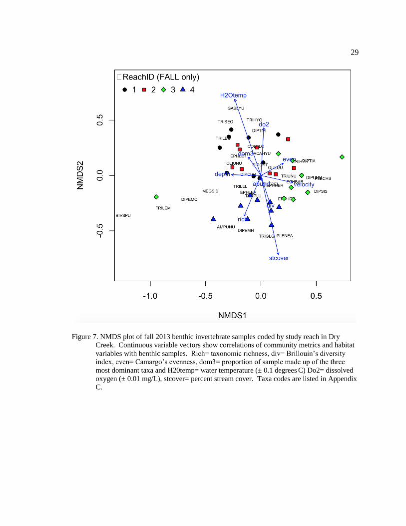
Figure 7. NMDS plot of fall 2013 benthic invertebrate samples coded by study reach in Dry
Creek. Continuous variable vectors show correlations of community metrics and habitat
variables with benthic samples. Rich= taxonomic richness, div= Brillouin’s diversity
index, even= Camargo’s evenness, dom3= proportion of sample made up of the three
most dominant taxa and H20temp= water temperature (± 0.1 degrees C) Do2= dissolved
oxygen (± 0.01 mg/L), stcover= percent stream cover. Taxa codes are listed in Appendix
C.

30
Table 7. Results from non-metric multidimensional scaling (NMDS) regression analysis and ANOVA of community metrics and
environmental variables among reaches. Data were summarized from 36 samples, collected in spring 2013, with each sample
representing a composited collection of 3 samples along a channel cross-section. Reaches listed from downstream to upstream. NMDS ANOVA
NMDS1 NMDS2 R2 p Reach 1 Reach 2 Reach 3 Reach 4
Variables
Vector
values
Vector
values
Metric
values
Metric
values
Metric
values
Metric
values F (3,32) p
Taxonomic richness 0.0804 -0.9968 0.4370 0.0002 37 40 44 45 7.9770 0.0004
Brillouin’s diversity 0.4418 -0.8971 0.0782 0.2922 0.2087 0.1847 0.1673 0.2137 4.6970 0.0079
Camargo’s evenness 0.1647 0.9863 0.1273 0.1320 2.3131 2.2453 2.2288 2.5135 4.3280 0.0114
Percent dominant
threea
-0.7117 0.7025 0.0371 0.5700 54% 65% 59% 51% 4.9440 0.0062
Mean
values
Mean
values
Mean
values
Mean
values
Water temperature
(OC)
0.6670 0.7450 0.5239 0.0001 15.067 15.033 13.367 12.967 22.730 <0.0001
Dissolved oxygen
(mg/L)
0.2953 -0.9554 0.0363 0.5693 9.4867 9.8400 9.2000 9.7967 32.040 <0.0001
Percent stream cover -0.9334 -0.3587 0.4555 0.0004 43% 35% 78% 70% 18.270 <0.0001
Depth (cm) 0.3379 -0.9412 0.1406 0.1072 1.6019 1.2944 1.6133 1.6389 0.6470 0.5910
Velocity (± cm· s-1) -0.7782 -0.6280 0.3195 0.0024 18.409 72.713 79.790 172.72 10.090 0.0001
a: Percentage of total individuals per reach comprised of the three most abundant taxa.

31
Table 8. Results from non-metric multidimensional scaling (NMDS) regression analysis and ANOVA of community metrics and
environmental variables among reaches. Data were summarized from 36 samples, collected in fall 2013 with each sample
representing a composited collection of 3 samples along a channel cross-section. Reaches listed from downstream to upstream. NMDS ANOVA
NMDS1 NMDS2 R2 p Reach 1 Reach 2 Reach 3 Reach 4
Variables
Vector
values
Vector
values
Metric
values
Metric
values
Metric
values
Metric
values F (3,32) p
Taxonomic richness -0.4080 -0.9130 0.2058 0.0332 43 41 44 46 0.5320 0.6640
Brillouin’s diversity 0.0898 -0.9960 0.0684 0.3500 0.1926 0.2239 0.2282 0.2140 0.4210 0.7390
Camargo’s evenness 0.9280 0.3725 0.0442 0.5123 2.3675 2.4514 2.5755 2.4825 0.0620 0.9800
Percent dominant
threea
-0.4424 0.8968 0.0523 0.4439 56% 59% 51% 55% 0.2630 0.8520
Mean
values
Mean
values
Mean
values
Mean
values
Water temperature
(O C)
-0.2580 0.9661 0.5521 0.0001 14.900 14.000 13.667 12.800 17.700 <0.0001
Dissolved oxygen
(mg/L)
0.0851 0.9964 0.2068 0.0337 10.737 10.947 10.263 10.213 7.3120 0.0007
Percent stream cover 0.1700 -0.9854 0.6189 0.0001 41% 43% 70% 81% 27.980 <0.0001
Depth (cm) -0.9956 -0.0943 0.1206 0.1431 1.2167 1.7222 1.8511 1.5856 1.5880 0.2120
Velocity (± cm· s-1) 0.9551 -0.2962 0.1195 0.1402 74.440 39.330 60.331 60.443 3.3870 0.0313
a: Percentage of total individuals per reach comprised of the three most abundant taxa.

32
Steelhead Diet Composition
A total of 68 taxa were identified in the steelhead diet samples (Appendix C).
Baetis, Ochrotrichia (Trichoptera: Hydroptillidae) and Chironomidae were the most
abundant taxa found in samples and represented 43% of the individuals enumerated.
Fourteen taxa that were present in diet samples were not found in benthic samples, and of
these taxa, seven had strictly terrestrial life stages (Appendix C). However, total
abundance of terrestrial invertebrates was relatively low and composed only 1.1% of diet
samples combined. When comparing diet metrics between reaches, percent dominant
three, biomass and abundance did not differ among reaches in the fall (Table 9).

33
Table 9. ANOVA analysis of the effect of reach on prey biomass, prey abundance, and percent of the diet composed of the three most
abundant taxa in diet samples of young of year steelhead. Up to 20 diet samples were collected per reach in fall 2013 from four
reaches in Dry Creek. The contiguous reaches extended from just downstream of Warm Springs Dam (reach 4) to the confluence
of the creek with the Russian River (reach 1).
Diet Metrics df
Sum of
squares
Mean
Square F p Mean values
Reach 1 Reach 2 Reach 3 Reach 4
Percent
dominant threea Reach 3 0.0398 0.0133 0.4180 0.7400
0.76938 0.80638 0.84739 0.66758
Residuals 82 2.5994 0.0317 - -
Biomass
Reach 3 0.0100 0.0033 0.7740 0.5120 77.038 66.511 18.255 35.754
Residuals 82 0.3546 0.0043 - -
Abundance Reach 3 1511 503.80 0.6500 0.5850 23.400 31.650 40.700 32.600
Residuals 82 63554 775.10 - -
a: Percentage of total individuals per reach comprised of the three most abundant taxa.

34
Diet composition differed among reaches (MRPP, A = 0.0257, p < 0.001),
although obvious groupings were not apparent in an NMDS plot (Figure 8). An
exception is that reach one samples were oriented along lower values on the NMDS 1
axis. Fifteen of the 68 taxa identified from diet samples were included among the ten
most abundant taxa found in each reach. Four of these taxa (Baetis, Ochrotrichia,
Chironomidae, and Lepidostoma) were found in all four reaches and were among the
most dominant taxa in each reach. In all reaches, diets were dominated by only a few
taxa. In reaches one, three and four, one taxa represented 25 percent or more of the
relative abundance found while in reach three, two taxa represented more than 25 (Table
10).

35
Figure 8. NMDS plot of fall 2013 steelhead (Oncorhynchus mykiss) diet samples coded by study
reach in Dry Creek. Taxa codes are listed in Appendix C.

36
Table 10. Relative numerical abundance of the ten most abundant taxa found in steelhead
(Oncorhynchus mykiss) diet samples collected in fall 2013, for each reach in Dry Creek,
Sonoma County, California. Reaches are shown in order from downstream to upstream. Reach 1 Reach 2
Taxa
Relative
Abundance Taxa
Relative
Abundance
Baetis (Ephemeroptera:
Baetidae)
0.33 Baetis 0.17
Hydropsyche (Trichoptera:
Hydropsychidae)
0.11 Chironomidae (Diptera) 0.12
Simulium (Diptera: Simulidae)
0.07 Ochrotrichia 0.09
Chironomidae
0.06 Antocha (Diptera: Tipulidae) 0.07
Lepidostoma (Trichoptera:
Lepidostomatidae)
0.06 Hydropsyche 0.07
Trichoptera
0.05 Isoperla (Plecoptera: Perlodidae) 0.06
Ochrotrichia (Trichoptera:
Hydroptillidae)
0.05 Tricorythodes (Ephemeroptera:
Leptohyphidae)
0.05
Epeorus (Trichoptera:
Heptageniidae)
0.04 Tanypodinae (Diptera:
Chironomidae)
0.04
Antocha
0.03 Lumbriculidae (Oligochaeta) 0.03
Lumbriculidae
0.03 Lepidostoma 0.03
Reach 3 Reach 4
Taxa
Relative
Abundance Taxa
Relative
Abundance
Ochrotrichia
0.25 Baetis 0.29
Chironomidae
0.11 Lepidostoma 0.14
Baetis
0.09 Ochrotrichia 0.11
Isoperla
0.09 Simulium 0.08
Antocha
0.08 Isoperla 0.07
Tricorythodes
0.06 Chironomidae 0.06
Lumbriculidae
0.05 Epeorus 0.04
Lepidostoma 0.04 Hydropsyche 0.03
Tanypodinae 0.03 Amphinemura (Plecoptera:
Nemouridae)
0.02
Culicoides (Diptera:
Empidinae)
0.03 Tricorythodes 0.02

37
In all reaches, correspondence between composition of diet and benthic
invertebrate samples was low (Bray-Curtis dissimilarity value > 0.6) for all comparisons
(Table 11), and ranks of relative abundance of invertebrate taxa match in steelhead diets
did not match ranks of relative abundance of invertebrate taxa in benthic samples (Figure
9). Further inconsistencies in relative abundances between diet composition and benthic
assemblages were also observed. Ochrotrichia was among the three most dominant taxa
in diets in three reaches (two, three and four) but was absent from the ten most abundant
taxa found in all reaches for benthic assemblages. Rhithrogena was among the two most
abundant benthic taxa in all reaches but was absent among diet composition of all
reaches. Optioservus made up over 25 percent of the benthic assemblage in reaches one
and two but were not abundant in corresponding diet composition. Baetis was the most
abundant benthic taxa in reach three diet samples but was ranked third in abundance in
diets, behind Ochrotrichia and Chironomidae (Figure 9).
Table 11. Results of Bray-Curtis dissimilarity index (0 = totally similar; 1 = totally dissimilar)
comparing steelhead diet samples to benthic invertebrate samples by reach in Dry Creek.
All samples were collected in the fall of 2013. Reaches are shown in order from
downstream to upstream.
Benthic
Invertebrate
Samples
Diet Samples Reach 1 Reach 2 Reach 3 Reach 4
Reach 1 0.7316 0.7012 0.8152 0.7122
Reach 2 0.7259 0.6905 0.8138 0.7633
Reach 3 0.6271 0.6851 0.8141 0.6434
Reach 4 0.6871 0.7120 0.8209 0.6486

38
Figure 9. Comparisons of relative abundance of the 10 most abundant taxa found in benthic
invertebrate samples and steelhead diet samples for each reach in Dry Creek. Samples
were collected in fall 2013. Reaches are shown in order from downstream to upstream.
Taxa codes are listed in Appendix C.

39
Some similarities between diet samples and benthic invertebrate samples were
observed. In reaches two and four, five of the ten most abundant taxa found in diets were
among the ten most abundant taxa found in benthic samples, and in reach three, four taxa
were abundant in both diet and fall benthic samples. Baetis and Chironomidae were
found among the ten most abundant taxa in diet composition and were among the four
most dominant taxa in benthic assemblages in all reaches. Baetis was the most dominant
taxa in diet composition of three reaches (one, two, and four) and Chironomidae was the
second most dominant in reaches two and three (Figure 9).
Steelhead Size and Prey Availability
Relative condition of fish in the fall differed among reaches (ANOVA, F(3, 943)
p<0.0008). Post-hoc comparisons using the Tukey’s HSD test indicated that reaches
three and four differed from reach one. Relative condition was the lowest in reach four
and increased downstream (Table 12). Length of fish also differed among reaches in the
fall (ANOVA, F (3, 943) p<0.0001) and increased in a downstream direction. Fish length
was similar between reach one and two, and between reach three and four; other pairwise
comparisons were significant (Table 13). Because steelhead diet metrics (prey biomass,
abundance, and percent of samples composed of the three most abundant taxa) did not
differ among reaches, linear regression to evaluate the effect of prey availability on
reach-specific differences in relative condition of fish was not conducted.

40
Table 12. Summary of relative condition of fish in fall 2013 from four contiguous reaches in Dry
Creek, and results of Tukey’s HSD post hoc comparison. Reaches extended from just
downstream of Warm Springs Dam (reach 1) to the confluence of the Dry Creek with the
Russian River (reach 4).
Relative Condition Tukey’s HSD
Reach Mean
Std.
Deviation N
(Reach vs.
Reach) p
1 0.9993 0.0652 534 1-2 0.9491
2 0.9916 0.0809 23 1-3 0.0046
3 0.9832 0.0591 292 1-4 0.0126
4 0.9774 0.0834 201 2-3 0.9401
2-4 0.7986
3-4 0.8728
Table 13. Summary of length (mm) of fish in fall 2013 from four contiguous reaches in Dry
Creek, and results of Tukey’s HSD post hoc comparison. Reaches extended from just
downstream of Warm Springs Dam (reach 1) to the confluence of Dry Creek with the
Russian River (reach 4).
Length Tukey’s HSD
Reach Mean
Std.
Deviatio
n N
(Reach vs.
Reach) p
1
105.3
7 18.856 534 1-2 0.7576
2
101.6
4 18.228 23 1-3 < 0.0001
3
90.31
3 15.367 292 1-4 < 0.0001
4
85.56
0 14.639 201 2-3 0.0177
2-4 0.0005
3-4 0.0870

41
DISCUSSION
Benthic Macroinvertebrate Assemblages
Findings supported my prediction that benthic invertebrate assemblages in Dry
Creek would differ among reaches and display a longitudinal trend in composition from
the dam to the confluence with the Russian River. However, counter to my expectation
that taxonomic richness would increase with distance downstream from the dam,
taxonomic richness was highest in reach four (nearest the dam). This may be attributable
to agricultural encroachment. Much of the lower three study reaches in Dry Creek are
encroached by agriculture while the reach four is less encroached. Zhang et al. (2013)
observed that species richness and diversity in streams decreased in farmland and areas
with high anthropogenic disturbance. In the Russian River watershed, vineyard and
exurban development have been associated with increased fine sediment inputs to
streams (Lohse et al. 2008). Fine sediments can decrease benthic invertebrate taxonomic
richness (Rabení et al. 2005, Zweig and Rabení 2001) and this could explain how factors
such as land use along the Dry Creek corridor can result in patterns that are at odds with
the expectation of increasing taxonomic richness with downstream distance from a dam.
However, differences in richness were not large (richness ranged from 45 to 37 taxa
among reaches in spring, and from 46-41 taxa in spring). Greater impacts to the benthic
macroinvertebrate fauna from input of fine sediments or other causes related to altered

42
land use may have been observed if sampling had been expanded to include depositional
habitats such as pools or backwaters, where fine sediments would be accumulated.
A primary tenet of the River Continuum Concept (Vannote et. al 1980) and the
Serial Discontinuity Concept (Ward and Stanford 1983) is that biotic sorting along
physical gradients in lotic systems with natural hydrologic regimes will lead to
longitudinal trends in richness and other community metrics of benthic invertebrates.
Although the hydrologic regime in Dry Creek is regulated and may not conform as
strongly as expected to this principle (e.g. trends may be more subtle), other gradients are
apparent and do conform to expectations of the River Continuum Concept. For example,
riparian shading was more extensive in the upstream most reaches of the study area,
which likely affected temperature and the type of invertebrates present. Grouping of
invertebrate assemblages by reach were associated with differences in canopy, with
canopy cover decreasing with distance downstream from the dam in both spring and fall.
The longitudinal differences in invertebrate assemblage corresponded by showing a shift
away from taxa that feed predominantly on riparian inputs of detrital material in the
headwaters, to those that are primarily fueled by in-stream (autochthonous) primary
production further downstream. This shift results when increased photosynthesis (due to
more light from reduced canopy) leads to increases in standing crops of algae and a
cascade of effects on invertebrate and vertebrate consumers. Increases in standing crops
of algae also provide a rapid turn-over, high-quality food resource utilized by scraping
insects, which increase in abundance relative to collecting insects feeding on detrital

43
material found in stream reaches with higher canopy cover (Vannote et al. 1980, Towns
1981, Feminella et al. 1989).
The strong seasonal variability in benthic invertebrate assemblages observed
potentially affected food availability for rearing juvenile salmonids over the course of the
year. Benthic invertebrate abundance can be higher or lower depending on the season
and therefore increase or decrease the number of prey items available to fish as food in
the drift. Rincón and Lobón-Cerviá (1997) identified seasonal changes in the benthic
macroinvertebrate community as the main factor determining seasonal flux in drift
composition in the River Negro in Brazil. The pattern of seasonal variation they found in
drift, with a winter minimum and a spring peak, closely matched the seasonal changes in
invertebrate abundance in benthic samples.
With the exception of stream cover, other environmental variables with which
seasonal grouping of samples by NMDS were associated included dissolved oxygen,
velocity, and temperature. This finding may give the impression that seasonal differences
in invertebrate assemblages were related to seasonal differences in characteristics of Dry
Creek. However, due to the highly regulated bottom (deep) releases from Warm Springs
Reservoir that remain relatively constant throughout the spring, summer and fall, changes
in these parameters downstream from the dam likely are not great enough to be
biologically relevant to invertebrate assemblages. Seasonal differences in structure of
invertebrate assemblages seen in Dry Creek more likely reflect expression of diverse life
histories of component species which have evolved over an evolutionary time scale,
rather than as a response to current environmental variables. Phenological changes in

44
overall assemblage structure of benthic macroinvertebrates generally correspond with
seasonal changes in photoperiod and temperature, which are key triggers of life history
transition (Hynes 1970, Becker 1973, Mackey 1977).
Steelhead Diet Composition
Invertebrate composition of fall steelhead diets differed among reaches but
differences were not closely associated with corresponding reach-specific benthic
invertebrate assemblages as expected. Taxa that clearly dominated the benthic
invertebrate assemblages were not among the most abundant taxa in corresponding diets.
However, up to half of the most dominant taxa present in reach-specific benthic
invertebrate assemblages were also present in corresponding diet compositions. These
results suggest that juvenile steelhead in Dry Creek are feeding selectively on some
benthic taxa, such as the mayfly Baetis. Dedual and Collier (1995) examined
relationships among invertebrate samples from the benthos, drift and diets of steelhead,
and found a correlation between invertebrate relative invertebrate abundance in the
benthos and drift. They also found a stronger relationship between relative abundances
invertebrates in trout stomachs and in the drift than between diets and benthos. This
relationship reflects the well-documented tendency of juvenile steelhead to feed
predominantly in the water column on drifting invertebrates of aquatic and terrestrial
origin (e.g. Nislow et al. 1998), and the differing propensity of benthic invertebrate taxa
to drift (e.g. Wilzbach et al. 1988, Rader 2011). Nislow etal. (1998) found stream
salmonids will only switch to foraging on the benthos when drift is reduced or not

45
available. If drift sampling were included in the present study, a stronger correspondence
between steelhead diets in Dry Creek may have been apparent.
Evidence to support the contention that drift-feeding is an important strategy for
juvenile steelhead comes strictly from observational data. However, because of
sustained, relatively high flows due to artificial releases from Warm Springs Reservoir it
is likely that drifting invertebrates are consistently available as a food source for juvenile
steelhead in mainstem Dry Creek. Taxa often found in the steelhead diets, especially
Baetis, Lepidostomatidae, Hydropsychidae and Simuliidae, are documented to have a
higher propensity to drift (Radar 2011) lending support to the contention that drift-
feeding was an important strategy for steelhead over the course of the study period.
However, Oligochaeta and Hydroptillidae larvae were among the most abundant taxa
found in steelhead diets but individuals of these taxa are typically not abundant in drift
and/or are not easily available to fish as a food source (ie. Oligochaeta bury themselves
into substrate) (Radar 2011). Based on this apparent paradox, further study on foraging
habits of steelhead in Dry Creek is warranted.
Steelhead Size and Prey Availability
Reach-specific differences in steelhead diet composition and reach-specific
differences in steelhead condition and length were different among reaches; however,
metrics used to represent diet composition (abundance, biomass, and percent of sample
composed of the three most abundant taxa) did not differ among reaches and therefore the
effect of prey availability on reach-specific differences in relative condition of steelhead

46
could not be assessed. Evidence from PIT tag detection data in Dry Creek suggests that
juvenile steelhead display a high degree of site fidelity over the course of the study period
and during a similar period in other years. This suggests that similarities of diet metrics
among reaches are unlikely to be caused by fish feeding in multiple reaches and therefore
homogenizing their diets.
Differences in reach-specific condition, body length and the observed reach-
specific differences in growth documented in a previous work (Manning and Martini-
Lamb 2014) may be attributed to the differences in stream temperatures between the
lower most and the upper reaches. If food supply is similar between the upper and lower
reaches, a few degrees difference in temperature could have a significant effect on growth
rates of trout under conditions of constant food consumption (Railsback and Rose 1999).
Hokanson et al. (1977) found that steelhead reared in 15.5oC water temperatures had 1%
higher specific growth rates (%weight/day) than fish reared in 12.5oC under controlled
settings where fish were fed excess rations in all treatments. Fall stream temperatures
measured at the time of the study were approximately 2o C higher in reach one than reach
four and differences in fish condition and length were most significant between the
upstream and downstream most reach.
Concern that dam-related effects on rearing habitat and prey availability may limit
the productivity of juvenile salmonids has prompted large-scale habitat enhancement
effort and it serves as the genesis of the present study. However, dam-related conditions
in Dry Creek may be increasing juvenile steelhead success in comparison with steelhead
in non-regulated systems in the region. Steelhead summer growth rates observed during

47
validation monitoring in Dry Creek were higher than those observed in other coastal
California streams (Hayes et al. 2008, Sogard et al. 2009). Longitudinal differences in
water temperature may be affecting reach-specific growth rates but bottom-water releases
(deep) from Warm Spring Dam maintained average water temperatures over the course of
this study that were within the optimal temperature range for maximum steelhead growth
rates (Richter and Kolmes 2005, Railsback and Rose 1999, Hokanson et al. 1977). In
addition, the stable hydrology in lower Dry Creek could be increasing juvenile steelhead
yields because stream connectivity is maintained, especially during the summer and early
fall months when non-regulated Mediterranean streams typically become disconnected
(Gasith and Resh 1999). The higher streamflows and year-round stream connectivity
could also be increasing food availability by increasing wetted area for maximum aquatic
invertebrate production and drift densities (Hayes et al. 2008). Gislason (1985) found
that under stable flow regimes, the standing crop of benthic invertebrates was greatly
enhanced and it potentially increased the survival and growth of fish dependent on insects
for food. In a study that manipulated flow rates (Harvey et al. 2006) steelhead growth
rates and invertebrates drift rates and concentration was higher in control groups where
streamflow was not decreased. Entry into the drift by benthic invertebrates can increase
with water velocity (Poff and Ward 1991; Borchardt 1993), as does the distance traveled
by some drifting invertebrates (Allan and Feifarek 1989). The results would be more
food in the form of drift at a higher stream discharges which may be another mechanism
leading to benefits in steelhead growth.

48
The data presented here suggest that land use may be having a negative impact on
the invertebrate diversity in mid and lower reaches of Dry Creek. A study on the over-
summer survival rates of juvenile steelhead in an un-regulated stream in Sonoma County
found that vineyard land use had a significant negative association with survival and that
higher stream discharge was an important mediator of steelhead rearing habitat
conditions (Grantham et al. 2012). This suggests that effects of land use might be greater
without the augmented stream flows currently present in Dry Creek. In light of climate
change and the recent California drought, maintaining the current streamflow regime in
mainstem Dry Creek holds promise as a way of providing water temperatures and food
production on a year-round basis Pacific Salmon salmonids in a region of California
where habitat for juvenile salmonids is becoming increasingly scarce (Gasith and Resh
1999).

49
RECOMMENDATIONS FOR FURTHER STUDY
The results of this study can serve as baseline data of the benthic invertebrate
assemblage and condition of fish in Dry Creek prior to habitat enhancement projects
currently being implemented. Once construction is complete, a follow-up is study is
recommended to compare how invertebrate assemblages and condition of fish change in
response to habitat enhancements.
Further studies are recommended to better understand steelhead feeding strategies
and the mechanism by which benthic invertebrates become accessible to foraging fish.
Sampling of drift, benthic, and terrestrial sources of food is also recommended with diet
sampling in the same time and location. In addition, bioenergetics modeling could shed
more light on the relationship between food and growth of steelhead and how differences
in temperature and habitat-specific energetic costs of foraging affect growth rates.

50
LITERATURE CITED
Allan, J. D., and B. P. Feifarek. 1989. Distances traveled by drifting mayfly nymphs:
factors influencing return to the substrate. Journal of the North American
Benthological Society 8:322–330.
Austin, M., and P. Greig-Smith. 1968. The application of quantitative methods to
vegetation survey: II. Some methodological problems of data from rain forest.
The Journal of Ecology:827-844.
Baumgärtner, D., and K. O. Rothhaupt. 2003. Predictive length–dry mass regressions for
freshwater invertebrates in a pre- alpine lake littoral. International Review of
Hydrobiology 88(5):453-463.
Barbour, M.T., J. Gerritsen, B. D. Synder, and J. B. Stribling. 1999. Rapid bioassessment
protocols for use in wadeable streams and rivers: periphyton, benthic
macroinvertebrates, and fish. Second Edition. EPA 841-B-99-002. U.S.
Environmental Protection Agency; Office of Water; Washington, D.C.
Bayley, P. B. 1991. The flood pulse advantage and the restoration of river- floodplain
systems. Regulated Rivers: Research & Management 6(2):75-86.
Becker, C. D. 1973. Development of Simulium (Psilozia) vittatum Zett.(Diptera:
Simuliidae) from larvae to adults at thermal increments from 17.0 to 27.0 C.
American Midland Naturalist:246-251.
Benke, A. C., A. D. Huryn, L. A. Smock, and J. B. Wallace. 1999. Length-mass
relationships for freshwater macroinvertebrates in North America with particular
reference to the southeastern United States. Journal of the North American
Benthological Society:308-343.
Bison, P. A., and R. E. Bilby. 1998. Organic matter and trophic dynamics. River Ecology
and Management: Lessons from the Pacific Coastal Ecoregion. Springer, New
York: 373-398.
Borchardt, D. 1993. Effects of flow and refugia on drift loss of benthic
macroinvertebrates: implications for habitat restoration in lowland streams.
Freshwater Biology 29:221–227.

51
Boulton, A., and L. Lloyd. 1992. Flooding frequency and invertebrate emergence from
dry floodplain sediments of the River Murray, Australia. Regulated Rivers:
Research & Management 7(2):137-151.
Breitenmoser-Würsten, C., and M. Sartori. 1995. Distribution, diversity, life cycle and
growth of a mayfly community in a prealpine stream system (Insecta,
Ephemeroptera). Hydrobiologia 308(2):85-101.
Brett, J. R. 1952. Temperature tolerance in young Pacific salmon, genus Oncorhynchus.
Journal of the Fisheries Research Board of Canada 9(6):265-323.
California Department of Water Resources (DWR). 2015. California Data Exchange
Center. Warms Springs (USACE) (WRS). http://cdec.water.ca.gov/cgi-
progs/queryMM?s=WRS&sensor_num=23&d=01/2014&span=12months
(December 22, 2015).
Camargo, J. 1993. Must dominance increase with the number of subordinate species in
competitive interactions? Journal of Theoretical Biology 161(4):537-542.
Cochran, W. G. 1977. Sampling techniques. John Wiley & Sons.
Collins, P. T. 1992. Length-biomass relationships for terrestrial Gastropoda and
Oligochaeta. American Midland Naturalist:404-406.
Cuneo, D. 2011. Initial Study and Mitigated Negative Declaration of Environmental
Impact. Sonoma County Water Agency, Santa Rosa, CA.
Dedual, M., and K. J. Collier. 1995. Aspects of juvenile rainbow trout (Oncorhynchus
mykiss) diet in relation to food supply during summer in the lower Tongariro
River, New Zealand. New Zealand Journal of Marine and Freshwater Research
29(3): 381-391.
Dill, L. M., R. C. Ydenberg, and A. H. Fraser. 1981. Food abundance and territory size in
juvenile Coho salmon (Oncorhynchus kisutch). Canadian Journal of Zoology
59(9):1801-1809.
Fausch, K. D. 1984. Profitable stream positions for salmonids: relating specific growth
rate to net energy gain. Canadian Journal of Zoology 62(3):441-451.
Feminella, J. W., M. E. Power, and V. H. Resh. 1989. Periphyton responses to
invertebrate grazing and riparian canopy in three northern California coastal
streams. Freshwater Biology 22(3):445-457.

52
Fessler, J. L., and H. H. Wagner. 1969. Some morphological and biochemical changes in
steelhead trout during the parr-smolt transformation. Journal of the Fisheries
Board of Canada 26(11):2823-2841.
Freeman, M. C., Z. H. Bowen, K. D. Bovee, and E. R. Irwin. 2001. Flow and habitat
effects on juvenile fish abundance in natural and altered flow regimes. Ecological
Applications 11(1):179-190.
Gasith, A., and V. H. Resh. 1999. Streams in Mediterranean climate regions: abiotic
influences and biotic responses to predictable seasonal events. Annual review of
ecology and systematics: 51-81.
Gislason, J. C. 1985. Aquatic insect abundance in a regulated stream under fluctuating
and stable diel flow patterns. North American Journal of Fisheries Management
5(1): 39-46.
Grant, J. W. A., and I. Imre. 2005. Patterns of density- dependent growth in juvenile
stream- dwelling salmonids. Journal of Fish Biology 67.sB: 100-110.
Grantham, T. E., D. A. Newburn, M. A. McCarthy, and A. M. Merenlender. 2012. The
role of streamflow and land use in limiting oversummer survival of juvenile
steelhead in California streams. Transactions of the American Fisheries Society
141(3): 585-598.
Growns, I., I. Reinfelds, S. Williams, and G. Coade. 2009. Longitudinal effects of a water
supply reservoir (Tallowa Dam) on downstream water quality, substrate and riffle
macroinvertebrate assemblages in the Shoalhaven River, Australia. Marine and
Freshwater Research 60(6):594-606.
Harvey, B. C., R. J. Nakamoto, and J. L. White. 2006. Reduced streamflow lowers dry-
season growth of rainbow trout in a small stream. Transactions of the American
Fisheries Society 135(4): 998-1005.
Hayes, S. A., et al. 2008. Steelhead growth in a small central California watershed:
upstream and estuarine rearing patterns. Transactions of the American Fisheries
Society 137(1): 114-128.
Hódar, J. 1997. The use of regression equations for the estimation of prey length and
biomass in diet studies of insectivore vertebrates. Miscellània Zoologica 20(2):1-
10.

53
Hokanson, K. E. F., C. F. Kleiner, and T. W. Thorslund. 1977. Effects of constant
temperatures and diel temperature fluctuations on specific growth and mortality
rates and yield of juvenile rainbow trout, Salmo gairdneri. Journal of the Fisheries
Board of Canada 34(5): 639-648.
Hopkirk, J., and P. Northen. 1980. Technical report on fisheries of the Russian River.
Prepared for the Sonoma County Planning Department, Santa Rosa, CA.
Hynes, H. B. N. 1970. The ecology of running waters, volume 555. Liverpool University
Press Liverpool.
Inter-Fluve. 2010. Final Current Conditions Report, Dry Creek from Warm Springs Dam
to the Confluence with the Russian River. Prepared for the Sonoma County Water
Agency.
Inter-Fluve. 2011. Draft Habitat Enhancement Feasibility Study Report, Dry Creek from
Warm Springs Dam to the Confluence with the Russian River. Prepared for the
Sonoma County Water Agency.
Inter-Fluve. 2012. Dry Creek Fish Habitat Enhancement: Conceptual Design Report, Dry
Creek: Warm Springs Dam to to the Russian River Sonoma County, CA. Prepared
for the Sonoma County Water Agency.
Johnston, T. A., and R. A. Cunjak. 1999. Dry mass–length relationships for benthic
insects: a review with new data from Catamaran Brook, New Brunswick, Canada.
Freshwater Biology 41(4):653-674.
Jop, K. M., and K. W. Stewart. 1987. Annual stonefly (Plecoptera) production in a
second order Oklahoma Ozark stream. Journal of the North American
Benthological Society:26-34.
Ligon, F. K., W. E. Dietrich, and W. J. Trush. 1995. Downstream ecological effects of
dams. Bioscience:183-192.
Lohse, K. A., D. A. Newburn, J. J. Opperman, and A. M. Merenlender. 2008. Forecasting
relative impacts of land use on anadromous fish habitat to guide conservation
planning. Ecological Applications 18:467–482.
Mackey, A. 1977. Growth and development of larval Chironomidae. Oikos:270-275.
J. Martini-Lamb and Manning, D.J., editors. 2014. Russian River Biological Opinion
status and data report year 2013-14. Sonoma County Water Agency, Santa Rosa,
CA.

54
Marchant, R., and G. Hehir. 2002. The use of AUSRIVAS predictive models to assess the
response of lotic macroinvertebrates to dams in south- east Australia. Freshwater
Biology 47(5):1033-1050.
McArdle, B. H., and M. J. Anderson. 2001. Fitting multivariate models to community
data: a comment on distance-based redundancy analysis. Ecology 82(1):290-297.
McCullough, D. A., G. W. Minshall, and C. E. Cushing. 1979. Bioenergetics of a stream
“collector” organism, Tricorythodes minutus (Insecta: Ephemeroptera) 1, 2.
Limnology and Oceanography 24(1):45-58.
Merritt, R., K. Cummins, and M. Berg. 2008. An introduction to the aquatic insects of
North America. Kendall Hunt, Dubuque, Iowa.
Méthot, G. et al. 2012. Macroinvertebrate size-mass relationships: how specific should
they be? Freshwater Science 31(3):750-764.
Minchin, P. R. 1987. An evaluation of the relative robustness of techniques for ecological
ordination. Pages 89-107 in Theory and models in vegetation science. Springer.
Miyasaka, H. et al. 2008. Relationships between length and weight of freshwater
macroinvertebrates in Japan. Limnology 9(1):75-80.
Murphy, B. R., and D. W. Willis. 1996. Fisheries techniques. Citeseer.Anderson, M. J.
2001. A new method for non- parametric multivariate analysis of variance.
Austral ecology 26(1):32-46.
National Marine Fisheries Service. 2008. Biological opinion for water supply, flood
control operations, and channel maintenance conducted by the U.S. Army Corps
of Engineers, the Sonoma County Water Agency, and the Mendocino County
Russian River Flood Control and Water Conservation Improvement District in the
Russian River Watershed. National Marine Fisheries Service, Long Beach, CA.
Nislow, K. H., C. Folt, and M. Seandel. 1998. Food and foraging behavior in relation to
microhabitat use and survival of age-0 Atlantic salmon. Canadian Journal of
Fisheries and Aquatic Sciences 55(1): 116-127.
Oksanen, J. et al. 2007. The vegan package. Community ecology package.
Petts, G. E., and M. Greenwood. 1985. Channel changes and invertebrate faunas below
Nant-Y-Moch dam, River Rheidol, Wales, UK. Hydrobiologia 122(1):65-80.

55
Pielou, E. 1967. The use of information theory in the study of the diversity of biological
populations. Pages 163-77 in Proc. Fifth Berkeley Symposium on Math. Stat. and
Prob.
Plafkin, J. L., M. T. Barbour, K. D. Porter, S. K. Gross, and R. M. Hughes. 1989. Rapid
bioassessment protocols for use in streams and rivers: benthic macroinvertebrates
and fish. Rapid bioassessment protocols for use in streams and rivers: Benthic
macroinvertebrates and fish. EPA.
Poff, N. L., and D. D. Hart. 2002. How dams vary and why it matters for the emerging
science of dam removal an ecological classification of dams is needed to
characterize how the tremendous variation in the size, operational mode, age, and
number of dams in a river basin influences the potential for restoring regulated
rivers via dam removal. Bioscience 52(8):659-668.
Poff, N. L., and J. V. Ward. 1991. Drift responses of benthic invertebrates to
experimental streamflow variation in a hydrologically stable stream. Canadian
Journal of Fisheries and Aquatic Sciences 48:1926–1936.
Power, M. E., W. E. Dietrich, and J. C. Finlay. 1996. Dams and downstream aquatic
biodiversity: potential food web consequences of hydrologic and geomorphic
change. Environmental management 20(6):887-895.
Rabení, C. F., K. E. Doisy, and L. D. Zweig. 2005. Stream invertebrate community
functional responses to deposited sediment. Aquatic Sciences 67(4): 395-402.
Rader, R.B. 2011. A functional classification of the drift: traits that influence invertebrate
availability to salmonids. CJFAS 54:111-1234.
Railsback, S. F., and K. A. Rose. 1999. Bioenergetics modeling of stream trout growth:
temperature and food consumption effects. Transactions of the American
Fisheries Society 128(2):241-256.
Richter, Ann, and S. A. Kolmes. 2005. Maximum temperature limits for Chinook, coho,
and chum salmon, and steelhead trout in the Pacific Northwest. Reviews in
Fisheries Science 13(1): 23-49.
Rincón, P. A., and J. Lobón-Cerviá. 1997. Temporal patterns in macroinvertebrate drift in
a northern Spanish stream. Marine and Freshwater Research 48(50): 455-464.
Sabo, J. L., J. L. Bastow, and M. E. Power. 2002. Length–mass relationships for adult
aquatic and terrestrial invertebrates in a California watershed. Journal of the North
American Benthological Society 21(2):336-343.

56
Sample, B. E., R. J. Cooper, R. D. Greer, and R. C. Whitmore. 1993. Estimation of insect
biomass by length and width. American Midland Naturalist:234-240.
Smith, D. G. 2001. Pennak's freshwater invertebrates of the United States: Porifera to
Crustacea. John Wiley & Sons.
Smock, L. A. 1980. Relationships between body size and biomass of aquatic insects.
Freshwater Biology 10(4):375-383.
Sogard, S. M., T. H. Williams, and H. Fish. 2009. Seasonal patterns of abundance,
growth, and site fidelity of juvenile steelhead in a small coastal California stream.
Transactions of the American Fisheries Society 138(3): 549-563.
Stanford, J. A., and J. V. Ward. 1979. Stream regulation in North America. Pages 215-
236 in The ecology of regulated streams. Springer.
Stanford, J. A., and J. V. Ward. 2001. Revisiting the serial discontinuity concept.
Regulated Rivers: Research & Management 17(4- 5): 303-310.
Stoffels, R. J., S. Karbe, and R. A. Paterson. 2003. Length- mass models for some
common New Zealand littoral- benthic macroinvertebrates, with a note on
within- taxon variability in parameter values among published models. New
Zealand Journal of Marine and Freshwater Research 37(2):449-460.
Towns, D. 1981. Effects of artificial shading on periphyton and invertebrates in a New
Zealand stream. New Zealand Journal of Marine and Freshwater Research
15(2):185-192.
Vannote, R. L., G. W. Minshall, K. W. Cummins, J. R. Sedell, and C. E. Cushing. 1980.
The river continuum concept. Canadian Journal of Fisheries and Aquatic Sciences
37(1):130-137.
Vinson, M. R. 2001. Long-term dynamics of an invertebrate assemblage downstream
from a large dam. Ecological Applications 11(3): 711-730.
Wang, L., D. Infante, J. Lyons, J. Stewart, and A. Cooper. 2011. Effects of dams in river
networks on fish assemblages in non- impoundment sections of rivers in
Michigan and Wisconsin, USA. River Research and Applications 27(4):473-487.
Ward, J. V., and J. A. Stanford. 1983. The serial discontinuity concept of lotic
ecosystems. Dynamics of lotic ecosystems: 29-42.

57
Wenzel, F., E. Meyer, and J. Schwoerbel. 1990. Morphometry and biomass determination
of dominant mayfly larvae (Ephemeroptera) in running waters. Archiv fur
Hydrobiologie 118(1):31-46.
Wilzbach, M.A., K.W. Cummins, and R.A. Knapp. 1988. Towards a functional
classification of stream invertebrate drift. Verh. Int. Ver. Limnol. 23:1244-1254.
Zhang, Y. et al. 2013. Relationships between macroinvertebrate communities and land
use types within different riparian widths in three headwater streams of Taizi
River, China. Journal of Freshwater Ecology 28(3):307-328.
Zimmerman, G. M., H. Goetz, and P. W. Mielke Jr. 1985. Use of an improved statistical
method for group comparisons to study effects of prairie fire. Ecology 66(2):606-
611.
Zweig, L. D., and C. F. Rabení. 2001. Biomonitoring for deposited sediment using
benthic invertebrates: a test on 4 Missouri streams. Journal of the North American
Benthological Society 20(4): 643-657.

58
APPENDIX A
Appendix A. Length-weight regression equations for aquatic life stages of invertebrates based on body length. The only exception was in
the case of Dixa (Diptera: Dixidae), which used head capsule width (HW). Equations are in the form of DM=a (Lb) unless
otherwise noted. DM = dry mass, L= body length and a and b are fitted coefficients. For regression equations that calculated ash-
free dry mass (AFDM) instead of DM, AFDM was converted to DM using the equation: 𝑀 = 𝐴𝐹𝐷𝑀 (100
100−%𝑎𝑠ℎ). If coefficients
from a different taxon were used to calculate DM, taxon is indicated in parenthesis.
Taxon a b % Ash Source
Insects
COLLEMBOLA (Insect) 0.0064 2.788 (Benke et al. 1999)
EPHEMEROPTERA 0.0071 2.832 (Benke et al. 1999)
Baetidae
Baetis 0.0095 2.440 (Johnston and Cunjak 1999)
Ephemerellidae
Serratella 0.0104 2.830 (Johnston and Cunjak 1999)
Heptageniidae 0.0111 2.440 (Johnston and Cunjak 1999)
Epeorus 0.0087 2.890 (Wenzel et al. 1990)
Rhithrogena 0.0138 2.560 (Breitenmoser-Würsten and Sartori
1995)
Leptophlebiidae
Paraleptophlebia 0.0094 2.510 (Johnston and Cunjak 1999)

59
Taxon a b % Ash Source
Leptohyphidae
Tricorythodes 0.0092 3.220 (McCullough et al. 1979)
ODONATA/ANISOPTERA 0.0088 2.787 (Benke et al. 1999)
PLECOPTERA 0.0094 2.754 (Benke et al. 1999)
Chloroperlidae
Suwallia 0.0065 3 (Benke et al. 1999)
Nemouridae
Amphinemura 0.0478 1.430 (Jop and Stewart 1987)
Perlidae
Hesperoperla 0.0099 2.879 (Benke et al. 1999)
Perlodidae
Isoperla 0.0552 1.790 (Jop and Stewart 1987)
Pteronarcyidae
Pteronarcys 0.3240 2.573 (Benke et al. 1999)
HEMIPTERA 0.0108 2.734 (Benke et al. 1999)
Corixidae 0.0031 2.904 (Benke et al. 1999)
Hebridae
Lipogomphus (Hemiptera) 0.0108 2.734 (Benke et al. 1999)

60
Taxon a b % Ash Source
MEGALOPTERA
Sialidae
Sialis 0.0037 2.753 (Benke et al. 1999)
TRICHOPTERA 0.0056 2.839 (Benke et al. 1999)
Glossosomatidae
Glossosoma 0.0082 2.958 (Benke et al. 1999)
Hydropsychidae
Hydropsyche 0.0046 2.926 (Benke et al. 1999)
Hydroptillidae
Ochrotrichiaa ln a= -4.41 2.57 (Baumgärtner and Rothhaupt 2003)
Lepidostomatidae
Lepidostoma 0.0079 2.649 (Benke et al. 1999)
Leptoceridae
Mystacides 0.0034 3.212 (Benke et al. 1999)
Rhyacophilidae
Rhycophila 0.0099 2.480 (Benke et al. 1999)
Sericostomatidae
Gomaga 0.0074 2.741 (Benke et al. 1999)
COLEOPTERA

61
Taxon a b % Ash Source
Curculionidae (Coleoptera) 0.0400 2.640 (Sabo et al. 2002)
Dytiscidae
Hydroporusa ln a= -2.784 2.500 (Smock 1980)
Elmidae
Optioservus 0.0740 2.879 (Benke et al. 1999)
Psephenidae
Psephenus 0.0123 2.906 (Benke et al. 1999)
DIPTERA 0.0025 2.692 (Benke et al. 1999)
Ceratopogonidae
Bezzia 0.0025 2.469 (Benke et al. 1999)
Chironomidae 0.00124 3.260 (Johnston and Cunjak 1999)
Tanypodinae 0.00562 2.000 (Johnston and Cunjak 1999)
Dixidae
Dixa (HW) 0.1110 3.775 (Miyasaka et al. 2008)
Empidinae 0.0054 2.546 (Benke et al. 1999)
Clinocera (Empidinae) 0.0054 2.546 (Benke et al. 1999)
Hemerodromia (Empidinae) 0.0054 2.546 (Benke et al. 1999)

62
Taxon a b % Ash Source
Simuliidae
Simulium 0.0060 2.810 (Johnston and Cunjak 1999)
Tabanidae
Tabanus 0.0050 2.681 (Benke et al. 1999)
Tipulidae 0.0029 2.681 (Benke et al. 1999)
Antocha (Tipulidae) 0.0029 2.681 (Benke et al. 1999)
Dicranota 0.0027 2.637 3.40 (Benke et al. 1999)
Hexatoma 0.0042 2.596 3 (Benke et al. 1999)
Non-insects
TURBELLARIA
Planariidae 0.0082 2.168 (Benke et al. 1999)
OLIGOCHAETA 0.0024 2.875 (Stoffels et al. 2003)
Lumbriculidae (Oligochaeta) 0.0024 2.875 (Stoffels et al. 2003)
GASTROPODA
Lymnidaea ln a= -4.76 3.190 (Baumgärtner and Rothhaupt 2003)
Physidaea (Lymnidae) ln a= -4.76 3.190 (Baumgärtner and Rothhaupt 2003)
Pomatiopsidaea (Lymnidae) ln a= -4.76 3.190 (Baumgärtner and Rothhaupt 2003)
Planobridaeb log a= -1.12 2.900 17.9 (Méthot et al. 2012)
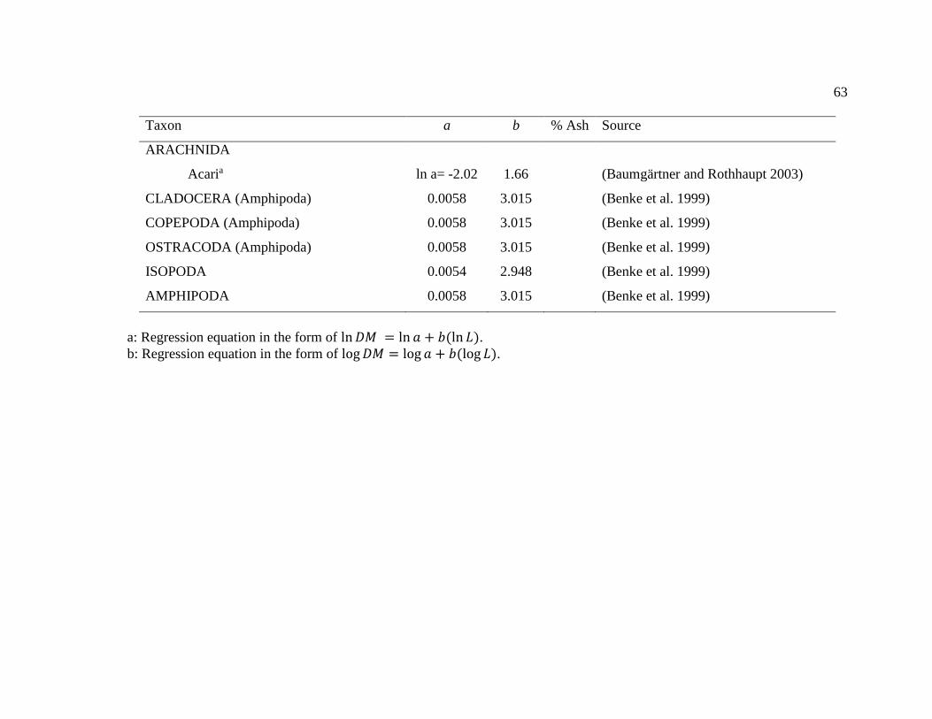
63
Taxon a b % Ash Source
ARACHNIDA
Acaria ln a= -2.02 1.66 (Baumgärtner and Rothhaupt 2003)
CLADOCERA (Amphipoda) 0.0058 3.015 (Benke et al. 1999)
COPEPODA (Amphipoda) 0.0058 3.015 (Benke et al. 1999)
OSTRACODA (Amphipoda) 0.0058 3.015 (Benke et al. 1999)
ISOPODA 0.0054 2.948 (Benke et al. 1999)
AMPHIPODA 0.0058 3.015 (Benke et al. 1999)
a: Regression equation in the form of ln 𝐷𝑀 = ln 𝑎 + 𝑏(ln 𝐿).
b: Regression equation in the form of log 𝐷𝑀 = log 𝑎 + 𝑏(log 𝐿).

64
APPENDIX B
Appendix B. Length-weight regression equations for adult life stages of invertebrates based on body length. The only exception was in the
case of Armadillidium (Isopoda: Armadillidae), which used head capsule width (HW). Equations are in the form of DM=a(Lb)
unless otherwise noted. DM = dry mass, L= body length and a and b are fitted coefficients. If coefficients from a different taxon
were used to calculate DM, taxon are indicated in parenthesis.
Taxon a b Source
Insects
EPHEMEROPTERA 0.014 2.49 (Sabo et al. 2002)
Baetidae
Baetis (Ephemeroptera) 0.014 2.49 (Sabo et al. 2002)
Leptohyphidae
Tricorythodes (Ephemeroptera)
0.014 2.49 (Sabo et al. 2002)
PLECOPTERA 0.26 1.69 (Sabo et al. 2002)
Perlodidae
Isoperla (Plecoptera)
0.26 1.69 (Sabo et al. 2002)
DERMAPTERA
0.598 2.387 (Hódar 1997)
TRICHOPTERA 0.01 2.9 (Sabo et al. 2002)
Hydropsychidae
Hydropsyche (Trichoptera)
0.01 2.9 (Sabo et al. 2002)
LEPIDOPTERA 0.012 2.69 (Sabo et al. 2002)

65
Taxon a b Source
COLEOPTERA
Carabidaea
2.755 -3.724 (Sample et al. 1993)
Coccinellidaea
3.867 -4.927 (Sample et al. 1993)
HYMENOPTERA
0.56 1.56 (Sabo et al. 2002)
Formicidaea
2.919 -4.727 (Sample et al. 1993)
DIPTERA
0.04 2.26 (Sabo et al. 2002)
Chironomidae (Nematocera) 0.01 1.57 (Sabo et al. 2002)
Simuliidae
Simulium (Nematocera)
0.01 1.57 (Sabo et al. 2002)
Tipulidae (Nematocera) 0.01 1.57 (Sabo et al. 2002)
Non-insects
GASTROPODA 0.969 0.529 (Collins 1992)
ARACHNIDA
Aranea 0.05 2.74 (Sabo et al. 2002)
ISOPODA
Armadillidae
Armadillidium (HW, Isopoda) 0.666 3.292 (Hódar 1997)
a: Regression equation in the form of log 𝐷𝑀 = 𝑏 + 𝑎(log 𝐿).

66
APPENDIX C
Appendix C. Invertebrate taxa identified from benthic samples and diet samples of juvenile
steelhead in Dry Creek, Sonoma County, California spring and fall 2013 and their
corresponding taxa codes. All taxa were collected in benthic samples and/or diet
samples.
Order Family Genus Taxa code
Sample
type
Insects
Coleoptera Carabidae Unknown COLCAUt Diet
Coleoptera Coccinellidae Unknown COLCOUt Diet
Coleoptera Curculionidae Unknown COLCUU Diet
Coleoptera Dytiscidae Hydroporus COLDYH Both
Coleoptera Elmidae Narpus COLELN Benthic
Coleoptera Elmidae Optioservus COLELO Both
Coleoptera Noteridae Pronoterus COLNOP Benthic
Coleoptera Psephenidae Psephenus COLPSP Both
Collembola Unknown Unknown COLUNU Both
Dermaptera Unknown Unknown DERUNUt Diet
Diptera Ceratopogonidae Bezzia DIPCEB Both
Diptera Ceratopogonidae Culicoides DIPCEC Benthic
Diptera Dixidae Dixa DIPDID Diet
Diptera Ceratopogonidae Forcipomyia DIPCEF Benthic
Diptera Chironomidae Tanypodinae
(tribe)
DIPCHT Both
Diptera Chironomidae Unknown DIPCHU Both
Diptera Empidinae Clinocera DIPEMC Both
Diptera Empidinae Hemerodromia DIPEMH Both
Diptera Empidinae Unknown DIPEMU Both

67
Order Family Genus Taxa code
Sample
type
Diptera Simuliidae Simulium DIPSIS Both
Diptera Tabanidae Tabanus DIPTAT Diet
Diptera Tanyderidae Unknown DIPTAU Benthic
Diptera Tipulidae Antocha DIPTIA Both
Diptera Tipulidae Dicranota DIPTID Both
Diptera Tipulidae Hexatoma DIPTIH Both
Diptera Unknown Unknown DIPUNU Both
Ephemeroptera Baetidae Baetis EPHBAB Both
Ephemeroptera Ephemerellidae Serratella EPHEPS Both
Ephemeroptera Heptageniidae Epeorus EPHHEE Both
Ephemeroptera Heptageniidae Rhithrogena EPHHER Both
Ephemeroptera Leptophlebiidae Paraleptophlebia EPHLEP Both
Ephemeroptera Leptohyphidae Tricorythodes EPHLET Both
Ephemeroptera Potamanthidae Anthopotamus EPHPOA Benthic
Ephemeroptera Unknown Unknown EPHUNU Both
Hemiptera Corixidae Unknown HEMCOU Both
Hemiptera Hebridae Lipogomphus HEMHEL Both
Hemiptera Unknown Unknown HEMUNU Both
Hymenoptera Formicidae Unknown HYMFOUt Diet
Hymenoptera Unknown Unknown HYMUNUt Both
Lepidoptera Unknown Unknown LEPUNUt Diet
Megaloptera Sialidae Sialis MEGSIS Both
Odonata Gomphidae Ophiogomphus ODOGOO Both
Plecoptera Chloroperlidae Suwallia PLECHS Both
Plecoptera Nemouridae Amphinemura PLENEA Both
Plecoptera Perlidae Calineuria PLEPECA Benthic

68
Order Family Genus Taxa code
Sample
type
Plecoptera Perlidae Hesperoperla PLEPEH Both
Plecoptera Perlodidae Isoperla PLEPEI Both
Plecoptera Pteronarcyidae Pteronarcys PLEPTP Both
Plecoptera Unknown Unknown PLEUNU Both
Trichoptera Brachycentridae Amocentrus TRIBRA Benthic
Trichoptera Calamoceratidae Heteroplectron TRICAH Benthic
Trichoptera Glossosomatidae Glossosoma TRIGLG Both
Trichoptera Hydropsychidae Hydropsyche TRIHYH Both
Trichoptera Hydroptillidae Ochrotrichia TRIHYO Both
Trichoptera Lepidostomatidae Lepidostoma TRILEL Both
Trichoptera Leptoceridae Mystacides TRILEM Both
Trichoptera Leptoceridae Oecetis TRILEO Benthic
Trichoptera Limnephilidae Onocosmoecus TRILIO Benthic
Trichoptera Odontoceridae Nerophilus TRIODN Benthic
Trichoptera Philopotamidae Wormalidia TRIPHW Benthic
Trichoptera Rhyacophilidae Rhycophila TRIRHR Both
Trichoptera Sericostomatidae Gomaga TRISEG Both
Trichoptera Unknown Unknown TRIUNU Both
Non-Insects
Acari Hydrachnidia Unknown ACAHYU Both
Amphipoda Unknown Unknown AMPUNU Both
Aranea Unknown Unknown ARAUNUt Both
Bivalva Sphaeriidae Unknown BIVSPU Benthic
Cladocera Unknown Unknown CLAUNU Both
Copepoda Unknown Unknown COPUNU Both

69
Order Family Genus Taxa code
Sample
type
Gastropoda Unknown Unknown GASUNUt Diet
Gastropoda Lymnidae Unknown GASLYU Both
Gastropoda Physidae Unknown GASPHU Diet
Gastropoda Planobridae Unknown GASPLU Both
Gastropoda Pomatiopsidae Unknown GASPOU Both
Isopod Unknown Unknown ISOUNU Both
Isopod Armadillidae Armadillidium ISOARAt Diet
Nemertea Tetrastemmatidae Prostoma NEMTEP Benthic
Nematoda Unknown Unknown NEMUNU Benthic
Oligochaeta Lumbriculidae Unknown OLILUU Both
Oligochaeta Unknown Unknown OLIUNU Both
Ostracoda Unknown Unknown OSTUNU Both
Turbellaria Planariidae Unknown TURPLU Both
t: Taxa with a strictly terrestrial life history.