comparison and sensitivity of odasi ocean analyses in the

Comparison and Sensitivity of ODASI Ocean Analyses in the Tropical Pacific

CHAOJIAO SUN

Global Modeling and Assimilation Office, NASA Goddard Space Flight Center, Greenbelt, and Goddard Earth Sciences andTechnology Center, University of Maryland, Baltimore County, Baltimore, Maryland

MICHELE M. RIENECKER

Global Modeling and Assimilation Office, NASA Goddard Space Flight Center, Greenbelt, Maryland

ANTHONY ROSATI, MATTHEW HARRISON, AND ANDREW WITTENBERG

Geophysical Fluid Dynamics Laboratory, Princeton, New Jersey

CHRISTIAN L. KEPPENNE, JOSSY P. JACOB, AND ROBIN M. KOVACH

Global Modeling and Assimilation Office, NASA Goddard Space Flight Center, Greenbelt, and Science Applications InternationalCorporation, Beltsville, Maryland

(Manuscript received 22 February 2006, in final form 22 September 2006)

ABSTRACT

Two global ocean analyses from 1993 to 2001 have been generated by the Global Modeling and Assimi-lation Office (GMAO) and Geophysical Fluid Dynamics Laboratory (GFDL), as part of the Ocean DataAssimilation for Seasonal-to-Interannual Prediction (ODASI) consortium efforts. The ocean general cir-culation models (OGCM) and assimilation methods in the analyses are different, but the forcing andobservations are the same as designed for ODASI experiments. Global expendable bathythermograph andTropical Atmosphere Ocean (TAO) temperature profile observations are assimilated. The GMAO analysisalso assimilates synthetic salinity profiles based on climatological T–S relationships from observations(denoted “TS scheme”). The quality of the two ocean analyses in the tropical Pacific is examined here.Questions such as the following are addressed: How do different assimilation methods impact the analyses,including ancillary fields such as salinity and currents? Is there a significant difference in interpretation ofthe variability from different analyses? How does the treatment of salinity impact the analyses? BothGMAO and GFDL analyses reproduce the time mean and variability of the temperature field comparedwith assimilated TAO temperature data, taking into account the natural variability and representationerrors of the assimilated temperature observations. Surface zonal currents at 15 m from the two analysesgenerally agree with observed climatology. Zonal current profiles from the analyses capture the intensityand variability of the Equatorial Undercurrent (EUC) displayed in the independent acoustic Dopplercurrent profiler data at three TAO moorings across the equatorial Pacific basin. Compared with indepen-dent data from TAO servicing cruises, the results show that 1) temperature errors are reduced below thethermocline in both analyses; 2) salinity errors are considerably reduced below the thermocline in theGMAO analysis; and 3) errors in zonal currents from both analyses are comparable. To discern the impactof the forcing and salinity treatment, a sensitivity study is undertaken with the GMAO assimilation system.Additional analyses are produced with a different forcing dataset, and another scheme to modify the salinityfield is tested. This second scheme updates salinity at the time of temperature assimilation based on modelT–S relationships (denoted “T scheme”). The results show that both assimilated field (i.e., temperature) andfields that are not directly observed (i.e., salinity and currents) are impacted. Forcing appears to have moreimpact near the surface (above the core of the EUC), while the salinity treatment is more important belowthe surface that is directly influenced by forcing. Overall, the TS scheme is more effective than the T schemein correcting model bias in salinity and improving the current structure. Zonal currents from the GMAOcontrol run where no data are assimilated are as good as the best analysis.

Corresponding author address: Dr. Chaojiao Sun, Code 610.1, Global Modeling and Assimilation Office, NASA Goddard SpaceFlight Center, Greenbelt, MD 20771.E-mail: [email protected]

2242 M O N T H L Y W E A T H E R R E V I E W VOLUME 135

DOI: 10.1175/MWR3405.1

© 2007 American Meteorological Society

MWR3405

1. Introduction

Ocean data assimilation has reached a level of ma-turity such that, with ocean observations available in atimely manner, ocean products are now regularly gen-erated for many applications. One important applica-tion of ocean data assimilation is the initialization ofclimate forecasts. The ocean’s thermal inertia providesthe memory for the climate system at seasonal andlonger time scales. The initialization of the ocean statetherefore plays a key role in the ability to forecast ElNiño with coupled models. To forecast El Niño, thethermal structure in the equatorial Pacific waveguidehas to be well represented. Coupled climate forecastsystems usually start with ocean initial conditions gen-erated by assimilating subsurface temperature data intoan ocean model driven by observed forcing. Alves et al.(2004) show that the sensitivity of forecasts to forcing ismuch reduced and forecast skills are improved wheninitial conditions are generated through assimilation,suggesting that the impact of wind error could be miti-gated by ocean subsurface data assimilation. In addi-tion to climate forecast initialization, assimilation isalso used to synthesize available observations into ananalysis of the historical climate record (e.g., Stammeret al. 2002; Carton and Giese 2006, manuscript submit-ted to J. Geophys. Res.).

Approaches to data assimilation vary in degrees ofsophistication. The experience in atmospheric assimila-tion seems to indicate that the effort expended in im-proving such details as forecast error covariances,model biases, observation representation errors, andthe quality control of observations may be more impor-tant than the sophistication of the assimilation tech-nique. For the atmosphere, covariance scales are oftenestimated by analysis of the innovations (observationminus forecast) or from the difference between fore-casts and corresponding analyses. Unfortunately, ex-cept for sea surface height (SSH) and sea surface tem-perature (SST), there are so few synoptic observationsof ocean fields available that the estimation of forecasterror covariances for the ocean is problematic.

Advances seem unlikely beyond the simple struc-tures used by, for example, Behringer et al. (1998) andRosati et al. (1997), if our estimation of the covariancestructure is based on differences between model fore-cast and observation. One possibility is to use en-sembles of ocean simulations (forecasts), which areformed by perturbations of forcing and/or perturba-tions of internal parameters, to assess the error struc-tures. These error structures then have a dynamical ba-sis for their anisotropy and heterogeneity. Such en-sembles have been used by Borovikov et al. (2005) in a

static mode and by Keppenne and Rienecker (2002) ina time-evolving ensemble Kalman filter (EnKF;Evensen 1994, 2003; Keppenne et al. 2005). The ques-tion is whether such details impact the analyses andsubsequent forecasts with any discernible significance.Here, we use the better exercised systems of optimalinterpolation (OI) and three-dimensional variationaldata assimilation (3DVAR) to address basic questionssuch as the following: How do different assimilationprocedures impact the analyses, including fields such assalinity and currents that are not observed and updatedby assimilation? Is there a significant difference in in-terpretation of the variability from different analyses?

Several studies have shown that salinity can play animportant role in the variability of the tropical oceans(e.g., Roemmich et al. 1994; Lukas and Lindstrom1991). Salinity could influence the stability of the watercolumn and heat buildup in the western equatorial Pa-cific, and have significant impact on the generation ofEl Niño and La Niña (Maes et al. 2005). Historically,both subsurface temperature and SSH assimilationhave been conducted in a univariate sequential assimi-lation system (e.g., OI or 3DVAR) where only tem-perature corrections have been made. The burden hasbeen on the model to modify the salinity and flow fieldsin accordance with the new temperature analysis. Inrecent years, evidence has emerged of the potential del-eterious effects of univariate sequential assimilation onboth temperature and salinity fields and hence on thedensity field in some assimilation systems (e.g., Ji et al.2000; Troccoli et al. 2002, 2003; Burgers et al. 2002; Bellet al. 2004). The salinity field can be severely degradedand result in artificially strong convection and verticalmixing when correcting temperature without a con-comitant correction in salinity (Derber and Rosati1989; Troccoli and Haines 1999). The degradation ofthe mass field then leads to poor flow fields (e.g., Vi-alard et al. 2003; Ricci et al. 2005).

Given the scarcity of salinity observations, salinitycorrections are usually made by reference to the tem-perature analysis (e.g., Troccoli et al. 2003), by relatingaltimeter data to temperature and salinity profiles (e.g.,Behringer et al. 1998; Segschneider et al. 2001), or bymore sophisticated multivariate schemes (e.g., Boro-vikov et al. 2005; Keppenne et al. 2005). While Seg-schneider et al. (2001) used altimeter data to providesynthetic temperature and salinity profiles, the in-creases in 6-month forecast skill appeared to be dueprimarily to improved correction of salinity rather thanto the use of altimeter data per se. Argo profiles of bothtemperature and salinity to 2000-m depth will likelysignificantly improve ocean analysis by updating tem-perature and salinity fields simultaneously.

JUNE 2007 S U N E T A L . 2243

As part of the Ocean Data Assimilation for Seasonal-to-Interannual Prediction (ODASI) consortium effort,assimilations have been run from 1993 to 2002 by vari-ous ODASI members, using the same forcing datasetand observation data streams to facilitate the intercom-parison of the results. The ODASI consortium was anactivity of the National Oceanic and Atmospheric Ad-ministration’s (NOAA’s) Climate Dynamics/Experi-mental Prediction (CDEP) program. The consortiumwas focused toward improving ocean data assimilationmethods and their implementation in support of fore-casts with coupled general circulation models. The con-sortium activities were coordinated across four themes:ocean data assimilation product intercomparisons, de-velopment of observational data streams; model sensi-tivity experiments, and validation of assimilation prod-ucts in forecast experiments. The ultimate goal was toaccelerate progress in improving coupled model fore-cast skill. The main participants were the Center forOcean–Land–Atmosphere Studies (COLA), Interna-tional Research Institute for Climate and Society (IRI),The Lamont-Doherty Earth Observatory (LDEO),NOAA’s National Centers for Environment Prediction(NCEP), NOAA’s Geophysical Fluid Dynamics Labo-ratory (GFDL), and the Global Modeling and Assimi-lation Office (GMAO) at the National Aeronautics andSpace Administration (NASA) Goddard Space FlightCenter.

Here we focus on two global ocean data assimilationsystems from GFDL and GMAO. These two systemsuse different global ocean general circulation models(OGCMs) and different assimilation methods. The pur-pose of this paper is to evaluate these two analyses from1993 to 2001 and investigate the importance of salinitytreatment. Furthermore, the impact of forcing is ex-plored by sensitivity experiments. Given the end appli-cation of interest, namely, seasonal climate forecasts,we focus the evaluation and comparisons on the tropi-cal Pacific.

This paper is organized as follows: the two oceanmodels used at GMAO and GFDL and datasets of forc-ing and observations are briefly described in section 2.In section 3, the two ocean data assimilation systemsare summarized. The two analyses from GMAO andGFDL are evaluated in section 4. Results from sensi-tivity experiments are discussed in section 5. We sum-marize the results and provide conclusions in section 6.

2. Ocean models and data

a. GMAO ocean model

The GMAO ocean model is the Poseidon globalOGCM (Schopf and Loughe 1995; Yang et al. 1999). It

is a finite-difference, reduced-gravity ocean model anduses a generalized vertical coordinate designed to rep-resent turbulent, well-mixed surface layers and nearlyisopycnal deeper layers. Spherical coordinates with astaggered Arakawa B grid are used in the horizontal.The prognostic variables are layer thickness, tempera-ture, salinity, and current components. The SSH field isdiagnostic.

Vertical mixing is parameterized through a Richard-son-number-dependent mixing scheme (Pacanowskiand Philander 1981) implemented implicitly. An ex-plicit mixed layer is embedded within the surface layersfollowing Sterl and Kattenberg (1994). For layerswithin the mixed layer, the vertical mixing and diffusionare enhanced to mix the layer properties through thedepth of the diagnosed mixed layer. A time-splittingintegration scheme is used whereby the hydrodynamicsare done with a short time step (15 min), but the ver-tical diffusion, convective adjustment, and filtering aredone with coarser time resolution (half daily). In thisstudy, the global resolution is 1/3° latitude � 5/8° lon-gitude, with 27 vertical layers.

b. GFDL ocean model

The GFDL Modular Ocean Model version 4(MOM4) is a finite-difference version of the oceanprimitive equations under the Boussinesq and hydro-static approximation. Here we summarize some basicinformation; details are available from Griffies et al.(2005) and Gnanadesikan et al. (2006). It uses sphericalcoordinates in the horizontal (tripolar grid; see Murray1996) with a staggered Arakawa B grid and the z co-ordinate in the vertical. The ocean surface boundary iscomputed as an explicit free surface. The meridionalresolution varies between 1° in the midlatitudes and1/3° in the Tropics to resolve the equatorial waveguide.The zonal resolution is 1°. There are 50 vertical levelswith 22 uniformly spaced in the upper 220 m. The thick-ness gradually increases to a value of 366 m at depth.Vertical mixing follows the nonlocal K-profile param-eterization (KPP) of Large et al. (1994). The horizontalmixing of tracers uses the isoneutral method pioneeredby Gent and McWilliams (1990). The horizontal mixingof momentum uses an anisotropic viscosity scheme thatproduces large viscosity in the east–west direction, butrelatively small viscosity in the north–south directionoutside of boundary currents, similar to that of Large etal. (2001).

c. Forcing and observation data

The common forcing dataset used by the ODASIconsortium (denoted “ODASI forcing”) includes the


NCEP Climate Data Assimilation System 1 (CDAS 1)daily mean surface fluxes and wind stress [with windstress climatology replaced by Atlas/Special Sensor Mi-crowave Imager (SSM/I) analyses], and Reynolds SSTto provide an additional constraint on SST evolution(Reynolds and Smith 1994; Reynolds et al. 2002).

The observations used in the assimilation are theglobal expendable bathythermograph temperature pro-files available from the National Oceanographic DataCenter (NODC) archive, and temperature profiles inTropical Atmosphere Ocean (TAO)/Triangle Trans-Ocean Buoy Network (TRITON)/Pilot ResearchMoored Array in the Tropical Atlantic (PIRATA) moor-ing data (http://www.pmel.noaa.gov/tao/; McPhaden etal. 1998) are from the TAO project Web site. Variousquality control procedures were implemented to ensurethe quality of the data.

3. The ocean data assimilation systems

Here we summarize the main characteristics of theGMAO and GFDL ocean data assimilation systems.The main parameters used in the two ocean data as-similation systems are shown in Table 1.

a. GMAO ocean data assimilation systems

The GMAO has developed a hierarchy of assimila-tion systems, from univariate OI (Troccoli et al. 2003)to multivariate OI (Borovikov et al. 2005) to the en-semble Kalman filter (Keppenne et al. 2005). Here theunivariate OI scheme used to initialize the GMAO’scoupled forecast system is evaluated.

The background-error covariance used in the OI isconstant in time. Here the anisotropic Gaussian func-tion depends only on the distance between forecast lo-cations:

Pf��, ��, �z� � C exp��

L��2

� ��

L��2

� ��z

Lz��,

where L� defines the zonal decorrelation scale, L� themeridional decorrelation scale, and Lz the verticaldecorrelation scale. In this application, L� � 1800 km,L� � 400 km in the equatorial waveguide, and Lz �50 m. The horizontal scales are consistent with thoseused by Ji et al. (1995). The value for L� is modulatedmeridionally as suggested by Derber and Rosati (1989)to shorten the covariance scales with latitude. For thebackground error covariance of salinity, the relevantscales are set to L� � 800 km, L� � 300 km in theequatorial waveguide, and Lz � 40 m. The model errorvariance is assumed to be homogeneous with a value of(0.7°C)2. The observational error variance is assumed

to be (0.5°C)2 to account for representation error inaddition to instrument error. Observation errors areassumed to be white in time and to have a decorrelationscale of 1500 km.

In addition to the temperature data assimilation, theGMAO system uses a separate univariate OI to providea corresponding salinity analysis. The salinity analysis isbased primarily on synthetic salinity profiles derivedfrom the observed temperature profiles and historicalT–S relationships from the Levitus and Boyer (1994)monthly climatologies. We refer to this scheme as the“TS scheme” hereafter. The observational error vari-ance of the synthetic salinity observations is set to 4times the forecast (or background) error variance. Thisallows correction of model bias in salinity, yet preservesinterannual variability of the salinity field inherent inthe model simulation and in the corresponding tem-perature data.

The assimilation window is 10 days, with data up to 5days before and 5 days after included with a temporaldecay of 20 days applied to the innovations, similar tothat of Alves et al. (2004). The assimilation is per-formed every 5 days.

b. GFDL ocean data assimilation system

The GFDL ocean data assimilation system uses the3DVAR implementation by Derber and Rosati (1989),with background error variance varying geographically(see also Rosati et al. 1997; Zhang et al. 2005). Onlytemperature profiles are assimilated. The assimilationwindow is 30 days, using data up to 15 days before and15 days after the assimilation time. The backgrounderror covariance matrix is constructed by multiplying auniform background variance �2

b to an equivalent cor-relation model (implemented by repeated applicationsof a Laplacian smoother, using a zonal scale xL and ameridional scale yL) as

��rx , ry� � exp�� rx

xL�2

� � ry

yL�2�,

TABLE 1. Main parameters used in the GMAO and GFDLassimilation systems.

GMAO GFDL

Assimilation method OI 3DVARObservation temperature error

(°C)0.5 0.5

Model temperature error (°C) 0.7 0.2Synthetic salinity observation

error200% of model

errorN/A

SSS relaxation time scale (days) 730 10SST relaxation time scale (days) 10 10

JUNE 2007 S U N E T A L . 2245

where rx and ry are the zonal and meridional distance,respectively, of the grid point to the observation loca-tion. The elliptic nature of the correlation structure iscontrolled by xL and yL. At the equator, xL is roughly700 km and yL is 50 km while the correlation structurearound 20°N(S) is roughly isotropic (see Zhang et al.2005). The background error variance, �2

b, is set to(0.2°C)2. The observational errors are assumed uncor-related and the error variance is based on the estimateof observed temperature variance, which is set to(0.5°C)2.

4. Analysis evaluation and validation

We first compare the temperature field from theGMAO and GFDL analyses with the assimilated TAOtemperature profiles at a mooring site as a consistencycheck. Then, independent data from various sourcesare compared with the analyses for more rigorous as-sessment of analysis performance. A simulation-onlyrun (without data assimilation) is also included for com-parison: the GMAO control run (denoted “GMAO-CTL”). Note that the GMAO-CTL uses a differentforcing (the same forcing used in the GMAO seasonalforecast system; denoted “GMAO forcing”) from theODASI forcing used in the GMAO and GFDL analy-ses. The comparison of the analyses with the controlhere is therefore qualitative. However, we will comparethe GMAO-CTL with analyses that use both forcings insection 5 to address the role of forcing.

a. Comparison with TAO temperature profiles at140°W

Here we compare the GMAO and GFDL tempera-ture analyses at a mooring location in the equatorialcentral Pacific with the assimilated TAO profiles. Fig-ure 1 shows the temperature time series from the analy-ses and TAO observations at 140°W on the equatorover the 9-yr period (1993–2001). Both GMAO andGFDL analyses agree well with the TAO observationsas expected. The GMAO-CTL exhibits the observedinterannual variability and the big warming event dur-ing the 1997/98 El Niño. However, it fails to capture therapid cooling event in the thermocline during the 1998La Niña (e.g., see the 20° and 16°C isotherms). This isnot because GMAO-CTL uses a different forcingdataset, since other GMAO analyses using the sameforcing capture this cooling event successfully (notshown).

The statistics of the analyses and observations areshown in Fig. 2. The time mean of the error (differencewith TAO temperature) is around 1°C (GMAO) and0.7°C (GFDL) in the area of the Equatorial Undercur-

rent (EUC), with a standard deviation (STD) of errorabout 0.8°C (GMAO) and 1.2°C (GFDL). To evaluatethe significance of these differences, we compare collo-cated conductivity–temperature–depth (CTD) andTAO measurements that are within 0.2° radius of eachother (as done by Borovikov 2005). The statistics areaveraged over northern and southern areas of Niño-3(5°S–5°N, 150°–90°W) and Niño-4 (5°S–5°N, 160°E to150°W), to account for the different characteristics ofthese areas (Fig. 3). The differences of collocated CTDand TAO reach 1°C in the EUC and about 0.2°C below(Fig. 4). If we interpret these differences as the repre-sentation error, we may conclude that the differencesbetween each analysis and TAO observation are com-parable to representation errors. The variability, repre-sented by the standard deviation of the temperaturetime series, is captured well in the two analyses, al-though the peak variability is slightly underestimated.

b. Comparison with Reverdin and OSCAR surfacecurrent climatology

The surface current estimates in the tropical Pacificare influenced primarily by the surface wind forcing.For example, Fevrier et al. (2000) compared 15-m zonalcurrent anomalies and thermocline depth anomalies inthe tropical Pacific from three OGCMs forced by dif-ferent wind stress products and found that the surfacecurrent depends strongly on the wind forcing product;however, parameterizations in surface layer physicsalso need to be improved to reduce the uncertainty insurface current estimates. Because of the role of advec-tion in SST variations (e.g., Borovikov et al. 2001), it isalso of interest whether the assimilation of the tempera-ture profile data impacts the surface current estimate.Unfortunately, few surface current measurements exist.The near-surface estimates from acoustic Doppler cur-rent profiler (ADCP) at the TAO moorings are notwithout error (e.g., Harrison et al. 2001), and the use ofdrifter estimates requires judicious interpolation andsmoothing to produce a time series useful for compari-son with the assimilation fields.

Here (Fig. 5) we compare climatologies of the zonalcurrent from GFDL and GMAO analyses with theReverdin et al. (1994) and Ocean Surface CurrentAnalyses—Real time (OSCAR) climatologies (Lager-loef et al. 1999; Bonjean and Lagerloef 2002). It shouldbe noted that the Reverdin climatology was computedover the 1987–92 period whereas the other climatolo-gies are computed over the 1993–2001 period. Theagreement between observations and analyses are gen-erally good. The seasonal variability of the current sys-tem, with an intense North Equatorial Counter Current(NECC) near 7°N in boreal fall and weak South Equa-


FIG. 1. Time series of temperature from TAO observations and model simulations (1993–2001) at 140°W on theequator. Model results are from the GMAO and GFDL analyses and a control run from GMAO model simulation underthe “GMAO forcing.” The model values have been sampled in the same way as the data (no model values are used whenthe corresponding data are missing).

JUNE 2007 S U N E T A L . 2247

Fig 1 live 4/C

torial Current (SEC) in spring is present in all the cli-matologies, as are the off-equatorial double maxima inthe SEC. However, the analyses also display some bi-ases. In the GFDL analysis, the western section of theSEC is too strong during summer and fall, and the EUChas surfaced during all seasons. In the GMAO analysis,both the SEC and the NECC are too strong along thewestern boundary and the surfaced EUC is slightly toostrong during summer and fall. The extension of theperiod of eastward surface flow is not a deficiency ofthe models [see the GMAO-CTL in Fig. 6 and the re-sults of Harrison et al. (2001), using a similar model asGFDL], but apparently of the assimilation. Even withthe same wind forcing (ODASI forcing), there are dif-ferences between the GMAO and GFDL surface cur-rent analysis estimates. It is noted that the OSCARproduct, showing eastward flow throughout the year atthe western equatorial boundary, is inconsistent withthe other estimates.

Pattern correlations (Tables 2 and 3) show most con-sistent agreements among the products in fall when thecurrents are strong and least consistent in spring whenthe currents are weak. The assimilation products agreeequally well with Reverdin and OSCAR in the summer,but better with OSCAR in the other seasons. TheGMAO analysis agrees best with the OSCAR productin winter and spring, while the GFDL analysis is in bestagreement in summer. The two analyses are in betteragreement with each other than with either dataset.

c. Comparison with TAO ADCP current profiles

Here we compare zonal current analyses with inde-pendent current data from ADCPs deployed at threeequatorial TAO moorings on the western (165°E), cen-tral (140°W), and eastern Pacific (110°W). For refer-ence, GMAO-CTL is also included in the comparisons.Figure 6 shows the time series of GFDL, GMAO,GMAO-CTL, and TAO zonal current from 1993 to2001. At 165°E in the western equatorial Pacific, bothanalyses have difficulty with the unusually strong andshallow EUC right after the 1997/98 El Niño, while theGMAO-CTL captures this strong event successfully, al-though it tends to be too strong in other years. The

←

FIG. 2. Statistics of analyses and control with respect to theequatorial TAO temperature data at 140°W, averaged over 1993–2001: (a) time–mean temperature profiles of TAO, GMAO-CTL,GFDL, and GMAO analyses; (b) time–mean error with respect toTAO; (c) STD of these monthly time series; and (d) STD of error(difference with respect to TAO). The model values have beensampled in the same way as the data (no model values are usedwhen the corresponding data are missing).


GMAO zonal current has about the right variability;however, the GFDL zonal current is generally tooweak. At 140°W, both the GMAO analysis andGMAO-CTL display the observed variability and EUCintensity. The current reversal during the 1997/98 ElNiño event is best represented in the control simula-tion. The GFDL analysis captures the observed struc-ture but the EUC is too shallow. At 110°W, both analy-ses are able to reproduce the zonal current structurewell. The control has difficulty in reproducing the ob-served EUC intensity.

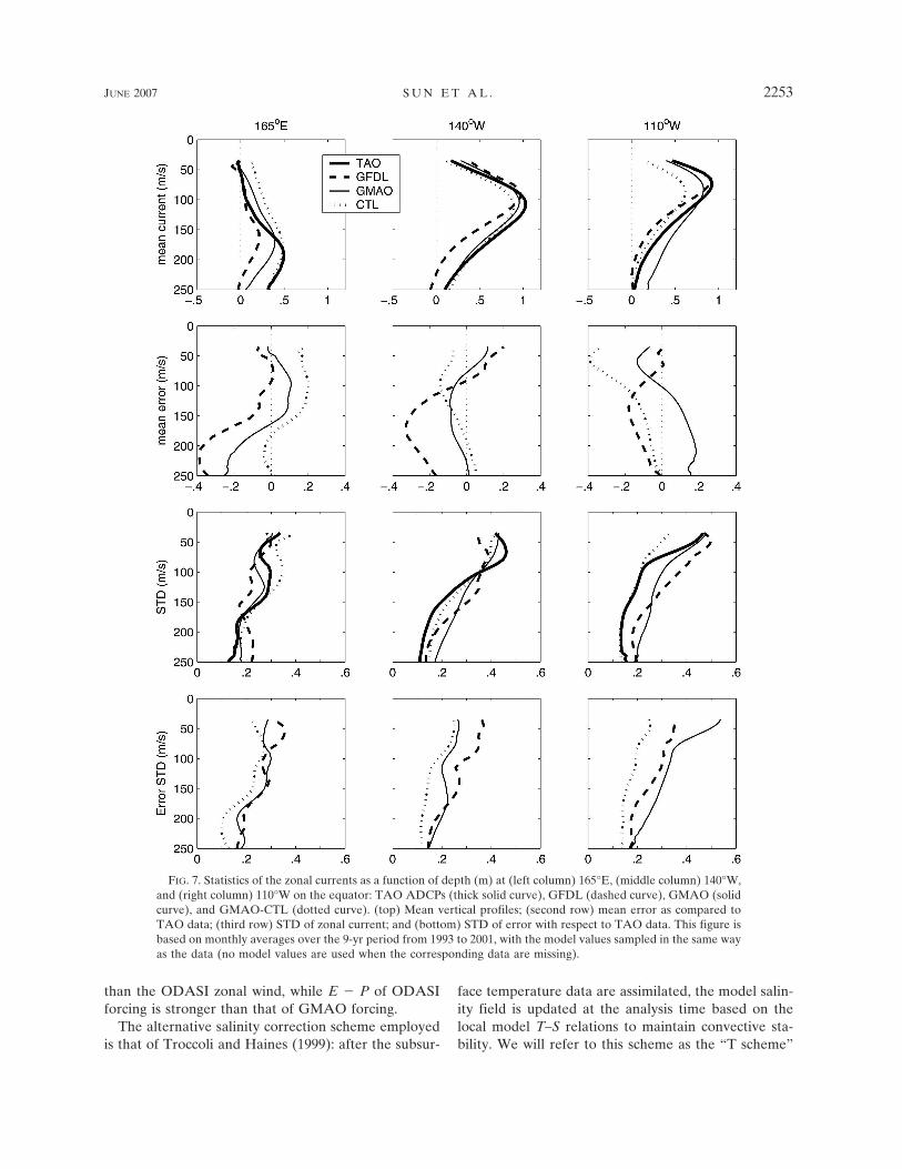
The statistics of the zonal current profiles averagedover the 9-yr period (1993–2001) are shown in Fig. 7. At165°E, the time mean of both GFDL and GMAO cur-rents match TAO observations well above 150 m, yetthey are both too weak in the EUC region below 150 m.The control run matches the lower part of EUC (below180 m) very well, but it is too strong elsewhere (up to0.20 m s�1). The variability in all the analyses and con-trol (shown by STD) are similar to the TAO currents,and the standard deviations of their errors are compa-rable. At 140°W, both the GMAO analysis andGMAO-CTL capture the observed time-mean currentstructure very accurately. Below 80 m, the GFDL cur-rent has a strong westward bias (up to 0.35 m s�1). At110°W, the control current is far too weak above 120 mand thus fails to capture the maximum of the EUC. Insection 5, it is shown that two other analyses producedby GMAO using the same forcing as the control havesimilar current structure at this location. The GFDLand GMAO currents are much closer to the TAO cur-rent in that area, although they both have biases below100 m (a westward bias in the GFDL analysis and aneastward bias in the GMAO analysis). At all three lo-cations, the STD of error is lowest for the control, sug-gesting that the error in the control current is mainly abias.

d. Comparison with TAO salinity profiles at 156°E

There are few salinity observations available in theocean to provide an adequate evaluation of the ocean

analyses. Here we compare our assimilation resultswith independent salinity data retrieved at an equato-rial TAO moored array at 156°E (Fig. 8). The data haveundergone quality control based on the quality flags,and obvious outliers are removed before comparison.Near the surface (above 50 m), both analyses tend to bemore saline than the observations and they are gener-ally in better agreement with each other than with theobservations, probably due to the fact that salinityvariations in the tropical Pacific are mainly driven byevaporation minus precipitation (E � P) forcing. Be-low 100 m, the GMAO salinity analysis is much closerto the TAO observation than the GFDL analysis, sug-gesting that the assimilation of climatological salinity inthe GMAO analysis helps to reduce salinity bias in themodel.

e. Comparison with TAO servicing cruises data

For years, the TAO servicing cruises have collectedCTD profiles and subsurface current measurements us-ing shipboard ADCPs during transects to and from theTAO mooring sites (Johnson et al. 2000, 2002). Thisdataset offers simultaneous measurements of tempera-ture, salinity, and currents. Here we compare our analy-ses with a gridded analysis of these independent datafrom 1994 to 1998 (Johnson et al. 2000). Comparisonstatistics are grouped separately for the northern andsouthern areas of Niño-3 and Niño-4 regions as definedin Fig. 3. The RMS difference (RMSD) between collo-cated model and cruise data in these four areas is shownin Fig. 9.

Both analyses generally improve the temperaturefield over the control, particularly between about 200and 500 m. As Borovikov et al. (2005) show, the rem-nant RMS error in the monthly mean comparisons isgreater than the higher-frequency variance in the con-trol or in the TAO moorings, so the remaining differ-ences are not likely due to a comparison of asynoptic“snapshots” from the cruises with monthly mean analy-ses.

The GMAO analysis is generally effective in correct-

FIG. 3. The four areas for which the RMSD statistics are computed. Areas 1 and 2 are thenorthern part of the Niño-4 (5°S to 5°N, 160°E to 150°W) and Niño-3 (5°S to 5°N, 150° to90°W) regions; areas 3 and 4 are the southern part of the Niño-4 and Niño-3 regions.

JUNE 2007 S U N E T A L . 2249

ing model salinity error, especially in the northern areasof Niño-3 and Niño-4 (areas 1 and 2). In contrast, theGFDL analysis, which does not treat salinity explicitly,has large salinity error in all areas, with the largest near1 psu in the southern Niño-4 region (area 3). Note thatthe degradation of the GMAO salinity analysis nearsurface, most apparent in the southern sections, is dueto the inappropriate use of the synthetic salinity data

within the mixed layer. Johnson et al. (2000) show thatthe isohaline layers in some of these CTD sections ex-tend to below 100 m, which are unlike the climatologyused for the synthetic salinity.

The errors in zonal currents from the two analysesand control are comparable except in the southernNiño-4 region (area 3), where the GFDL current hasslightly larger error below the thermocline. The fact

FIG. 4. STD (solid) and time mean (dashed) of the difference in collocated CTD and TAOmeasurements for the (upper) northern and (lower) southern areas of (right) Niño-3 and (left)Niño-4 regions. The CTD measurements are from TAO servicing cruises conducted duringDecember 1986 to December 1999. The TAO measurements are from the TAO moorings thatare collocated with the CTD casts. The collocation requirement is that the measurements weretaken within 0.2° lat and lon and on the same date. The number of profiles in each area is59 (57) in the Niño-3 region north (south) of the equator and 84 (72) in the Niño-4 regionnorth (south) of the equator.


that the control currents are as good as or even slightlybetter than analysis currents (but not in area 1) is acommon phenomenon in ocean analysis systems whenonly temperature data are assimilated. There could beseveral reasons. One is that the tropical Pacific ismainly wind driven, and both models are well tuned tosimulate the current structure well without assimilation.The assimilation of temperature introduces an imbal-ance in the model, and a correction is needed to bringthe model back to geostrophic balance (e.g., Burgers etal. 2002; Bell et al. 2004; Ricci et al. 2005). Anotherreason that the control is slightly better than theGMAO analysis current is hinted in the next section:the TS-scheme analysis using the same GMAO forcingas the control produces as good currents as the control.We elaborate further in section 5b.

5. Sensitivity analysis

In ocean state estimation, data assimilation helps tocompensate for errors in the surface forcing fields aswell as the initial conditions. We have seen from theprevious section that even with the same forcing fieldsand observation dataset, there are differences in theocean analyses generated with different models and as-similation methods. Here we explore the sensitivity ofthe analysis to the choice of forcing data. Given theimportance of correcting salinity during temperature-only assimilation, we also explore the sensitivity of theanalysis to the method of salinity correction. These sen-sitivity experiments are performed with the GMAO as-similation system.

The second set of forcing (i.e., GMAO forcing) is

FIG. 5. Seasonal climatology of 15-m zonal current from Reverdin et al. (1994), OSCAR, GMAO, and GFDL analyses. The Reverdinclimatology is representative of the period from January 1987 to April 1992. The dashed blue line indicates the equator. (top to bottom)Summer, fall, winter, and spring.

JUNE 2007 S U N E T A L . 2251

Fig 5 live 4/C

that used in the ocean initialization for the GMAOcoupled model forecasts (e.g., Vintzileos et al. 2003,2005). The forcing comprises SSM/I-derived time-varying wind stress (Atlas et al. 1996), Global Precipi-tation Climatology Project (GPCP) monthly mean pre-cipitation (Adler et al. 2003), NCEP CDAS 1 short-wave radiation (for penetrating radiation) and latent

heat flux (for evaporation), and Reynolds and Smith(1994) weekly SST. A comparison of zonal wind stressand freshwater flux (E � P) from ODASI forcing withthose of GMAO forcing at the equator over the 1993–2001 time period is shown in Fig. 10. The seasonal andinterannual variations in the two datasets are consis-tent. However, GMAO zonal wind is often stronger

FIG. 6. The time series of zonal current at 165°E, 140°W, and 110°W on the equator as a function of depth (m)from the TAO observations and models (the GFDL and GMAO analyses, and the GMAO-CTL). The white lineis the zero contour line and the black line is the 1 m s�1 contour line. The model values are sampled in the sameway as the data (i.e., no model values are used when the corresponding data are missing).

TABLE 2. Summer/fall seasonal climatology pattern correlationsof Reverdin, OSCAR, GMAO, and GFDL analyses. Note thatthe correlations above the diagonal are for the summer season,and the correlations below the diagonal are for the fall season.

Reverdin OSCAR GMAO GFDL

Reverdin 1.0000 0.8243 0.7235 0.7946OSCAR 0.8455 1.0000 0.7532 0.7497GMAO 0.7412 0.8510 1.0000 0.7838GFDL 0.7300 0.8250 0.8887 1.0000

TABLE 3. Winter/spring seasonal climatology pattern correla-tions of Reverdin, OSCAR, GMAO, and GFDL analyses. Notethat the correlations above the diagonal are for the winter season,and the correlations below the diagonal are for the spring season.

Reverdin OSCAR GMAO GFDL

Reverdin 1.0000 0.7787 0.7647 0.6655OSCAR 0.6224 1.0000 0.8406 0.7823GMAO 0.6017 0.7455 1.0000 0.8399GFDL 0.6274 0.6476 0.7560 1.0000


Fig 6 live 4/C

than the ODASI zonal wind, while E � P of ODASIforcing is stronger than that of GMAO forcing.

The alternative salinity correction scheme employedis that of Troccoli and Haines (1999): after the subsur-

face temperature data are assimilated, the model salin-ity field is updated at the analysis time based on thelocal model T–S relations to maintain convective sta-bility. We will refer to this scheme as the “T scheme”

FIG. 7. Statistics of the zonal currents as a function of depth (m) at (left column) 165°E, (middle column) 140°W,and (right column) 110°W on the equator: TAO ADCPs (thick solid curve), GFDL (dashed curve), GMAO (solidcurve), and GMAO-CTL (dotted curve). (top) Mean vertical profiles; (second row) mean error as compared toTAO data; (third row) STD of zonal current; and (bottom) STD of error with respect to TAO data. This figure isbased on monthly averages over the 9-yr period from 1993 to 2001, with the model values sampled in the same wayas the data (no model values are used when the corresponding data are missing).

JUNE 2007 S U N E T A L . 2253

hereafter. There is no assimilation in the top layer; themodel SST is relaxed to the Reynolds and Smith (1994)weekly SST product, with a seasonally and spatiallyvarying relaxation time scale derived from Comprehen-sive Ocean–Atmosphere Data Set (COADS) data. Sur-face salinity is relaxed to Levitus and Boyer (1994) cli-matology with an e-folding decay time scale of 2 yr.Salinity within the mixed layer is not updated in this Tscheme.

The GMAO experiments evaluated here are denoted

GMAO-T and GMAO-TS for the experiments usingGMAO forcing, and ODASI-T and ODASI-TS (this isthe GMAO analysis used in comparison with GFDLanalysis in the previous section) for the experimentsusing ODASI forcing (see Table 4). GMAO-CTL isincluded for comparison.

a. Comparison with TAO temperature profiles at 140°W

Here we compare GMAO temperature analyses withdependent data from the TAO mooring at 140°W on

FIG. 8. Time series of monthly mean salinity time series at 156°E on the equator from TAOobservations, GFDL, and GMAO analyses. The correlations between the GFDL and GMAOanalyses are displayed at the lower right-hand corner of each panel.


the equator (Fig. 11, similar to Fig. 2), similar to section4a. The mean temperature profiles from the GMAOanalyses (averaged over the 9-yr period from 1993 to2001) agree with the TAO observation (Fig. 11a). How-

ever, they are slightly too warm in the thermocline.Both TS experiments have slightly larger biases thanthe corresponding T experiments (Fig. 11b). This is notsurprising since the assimilation of synthetic salinity in

FIG. 9. RMSD of (top) temperature, (middle) salinity, and (bottom) zonal current between each of the model runs (GFDL analysis,GMAO control, and analyses) and observations from TAO servicing cruises (for the 5-yr period 1994–98) as a function of depth (m),averaged over the northern and southern Niño-3 and Niño-4 regions as defined in Fig. 3. Note that the x-axis scale for salinity in area3 is from 0 to 1 psu, and is twice as large as the scale for the other areas.

JUNE 2007 S U N E T A L . 2255

TS experiments could cause the analysis to deviatefrom the model temperature structure. All analysescapture the temporal variability well, with only a slightunderestimation of the peak variability (Fig. 11c). The

control underestimates the variability in the upper ther-mocline (above 120 m) and has the largest error STD.The standard deviations of differences are similar forall analyses (Fig. 11d). The GMAO analysis system em-ploys incremental adjustment of the model’s oceanstate through incremental analysis update (IAU;Bloom et al. 1996). This, in combination with the driftof the model forecast between analysis times, couldlead to RMS errors larger than the a priori error esti-mates for the background and observations.

b. Comparison with TAO ADCP current profiles

Similar to section 4c, the GMAO current analysesare compared with independent ADCP observations

TABLE 4. Summary of experiments.

Expt Assimilation method Forcing

GFDL 3DVAR, assimilating T only ODASIODASI-T OI, assimilating T only ODASIODASI-TS OI, assimilating T and S ODASIGMAO-T OI, assimilating T only GMAOGMAO-TS OI, assimilating T and S GMAOGMAO-CTL No assimilation GMAO

FIG. 10. Comparison of GMAO and ODASI forcing at the equatorial Pacific (140°E to 100°W) from 1993 to 2002. (a) ODASI zonalwind stress (N m�2); (b) GMAO zonal wind stress (N m�2); (c) ODASI freshwater flux, E � P (mm day�1); and (d) GMAO freshwaterflux, E � P (mm day�1).


Fig 10 live 4/C

made at three TAO moorings on the equator: 140°W,110°W, and 165°E (Fig. 12, similar to Fig. 7). In thecentral and eastern equatorial Pacific (140° and110°W), we find that the mean current above the EUCcore from GMAO analyses is mostly influenced byforcing rather than the treatment of salinity (Fig. 12,middle and right columns): the biases from analysesusing the same forcing are similar. Below the EUCcore, the biases from analyses using the same salinityupdate scheme are similar, with the TS scheme havingsmaller biases. The assimilation of climatological salin-ity effectively reduces the eastward bias below the EUCcore present in the two T-scheme analyses. This sug-gests that the role of forcing becomes less importantbelow the undercurrent core. In the western equatorialPacific (165°E), the current structure appears to bemore sensitive to the salinity treatment in the analysesthan the forcing used (Fig. 12, left). The two analysesusing the TS scheme have smaller mean error than theother two analyses using the T scheme. However, belowabout 160 m, the westward bias in the TS analyses isslightly larger than that in the control and T analyses.The reason for this result is not clear.

In summary, there is an overall good agreementamong the analyses, control, and TAO current obser-vations. The TS scheme generally produces similar cur-rents to the T scheme under the same forcing in thesurface (above the undercurrent core). However,deeper currents from the TS scheme tend to improveupon those from the T scheme, regardless of the forcingused, according to both mean and RMS error measures(except in the western Pacific). This seems to indicatethat forcing is the dominant factor in determining thedirection and magnitude of the near-surface currents(above 150 m or so), while the salinity treatment hasstrong impact on the deeper currents. The zonal currentfrom the GMAO control run is too weak in the under-current core (except at 165°E), but it is closer to theTAO observations below the core. Interestingly, eachanalysis tends to degrade the zonal current below theundercurrent core.

The results are consistent with the suggestion of Vi-alard et al. (2003) and Ricci et al. (2005), who foundthat the model bias in the salinity from the T scheme

←

FIG. 11. Statistics of GMAO analyses and CTL compared withthe equatorial TAO temperature data at 140°W: (a) Climatologi-cal temperature profiles of TAO, GMAO control, and GMAOanalyses, averaged over 1993–2001; (b) mean error of analysesand CTL with respect to TAO; (c) STD of the temperaturemonthly time series; and (d) STD of error with respect to TAO.

JUNE 2007 S U N E T A L . 2257

Fig 11 live 4/C

induced the downwelling of the eastward-flowing EUC,resulting in an eastward bias below the EUC core. TheT scheme, which relies on the model T–S relationshipto adjust salinity, is not capable of correcting the bias inthe model salinity field. Ricci et al. (2005) also foundthat at 140° and 110°W, the scheme that accounts for

salinity impacts produced smaller eastward bias belowthe core of EUC as compared to the scheme that doesnot correct the salinity bias. This suggests that salinitycorrection is more important at depths that are not di-rectly influenced by surface forcing. Another reasonthat the salinity adjustments help more at depth is that

FIG. 12. Same as in Fig. 7, except that the analyses are different: TAO ADCPs (black solid line), ODASI-TS (redsolid line), GMAO-TS (blue solid line), ODASI-T (red dashed line), GMAO-T (blue dashed line), and theGMAO-CTL (black dashed line).


Fig 12 live 4/C

the integrated effect of the density gradients growslarger with depth.

c. Comparison with TIWE cruise ADCP currentprofiles at 140°W

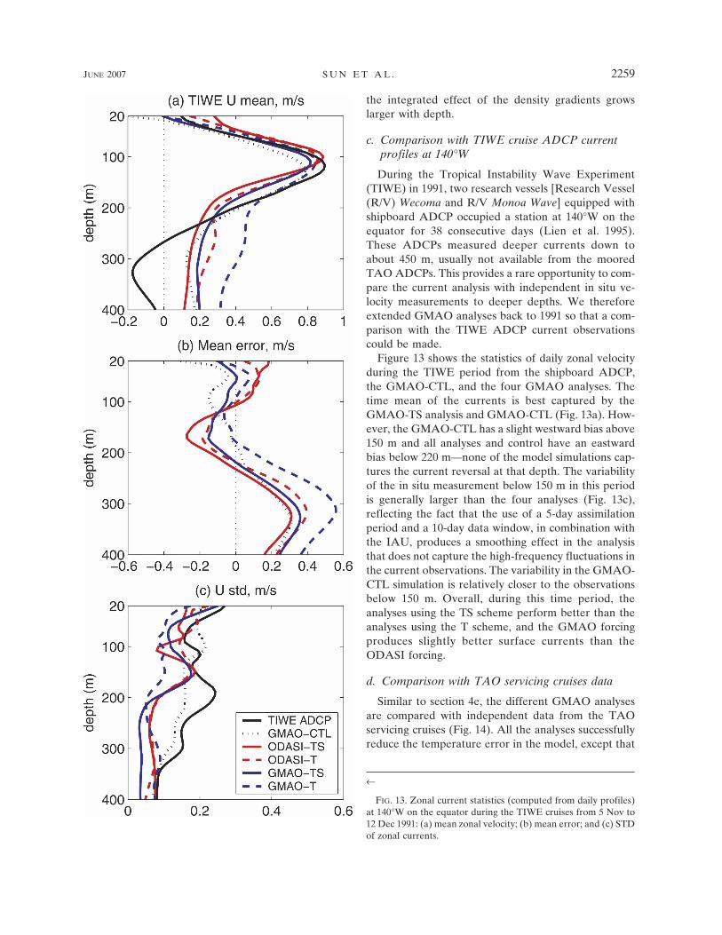
During the Tropical Instability Wave Experiment(TIWE) in 1991, two research vessels [Research Vessel(R/V) Wecoma and R/V Monoa Wave] equipped withshipboard ADCP occupied a station at 140°W on theequator for 38 consecutive days (Lien et al. 1995).These ADCPs measured deeper currents down toabout 450 m, usually not available from the mooredTAO ADCPs. This provides a rare opportunity to com-pare the current analysis with independent in situ ve-locity measurements to deeper depths. We thereforeextended GMAO analyses back to 1991 so that a com-parison with the TIWE ADCP current observationscould be made.

Figure 13 shows the statistics of daily zonal velocityduring the TIWE period from the shipboard ADCP,the GMAO-CTL, and the four GMAO analyses. Thetime mean of the currents is best captured by theGMAO-TS analysis and GMAO-CTL (Fig. 13a). How-ever, the GMAO-CTL has a slight westward bias above150 m and all analyses and control have an eastwardbias below 220 m—none of the model simulations cap-tures the current reversal at that depth. The variabilityof the in situ measurement below 150 m in this periodis generally larger than the four analyses (Fig. 13c),reflecting the fact that the use of a 5-day assimilationperiod and a 10-day data window, in combination withthe IAU, produces a smoothing effect in the analysisthat does not capture the high-frequency fluctuations inthe current observations. The variability in the GMAO-CTL simulation is relatively closer to the observationsbelow 150 m. Overall, during this time period, theanalyses using the TS scheme perform better than theanalyses using the T scheme, and the GMAO forcingproduces slightly better surface currents than theODASI forcing.

d. Comparison with TAO servicing cruises data

Similar to section 4e, the different GMAO analysesare compared with independent data from the TAOservicing cruises (Fig. 14). All the analyses successfullyreduce the temperature error in the model, except that

←

FIG. 13. Zonal current statistics (computed from daily profiles)at 140°W on the equator during the TIWE cruises from 5 Nov to12 Dec 1991: (a) mean zonal velocity; (b) mean error; and (c) STDof zonal currents.

JUNE 2007 S U N E T A L . 2259

Fig 13 live 4/C

the T-scheme analyses are worse than the control below500 m. The reduction of model salinity error by the TSscheme below the thermocline is most prominent in thenorthern sections of Niño-3 and Niño-4 (areas 1 and 2).The errors in zonal currents are smallest in the GMAO-

TS analysis and GMAO-CTL. ODASI-TS analysis isalmost as good except near the surface, which is prob-ably due to slightly larger error in ODASI wind forcing.Both T-scheme analyses have larger errors below thesurface in all four regions. As was found from the TAO

FIG. 14. RMSD of (top) temperature, (middle) salinity, and (bottom) zonal current between model runs and observations from TAOservicing cruises (for the 5-yr period 1994–98) as a function of depth (m), averaged over the northern and southern Niño-3 and Niño-4regions as shown in Fig. 3.


Fig 14 live 4/C

mooring comparison, the TS scheme produces moreaccurate zonal currents than the T scheme. The Tscheme cannot by itself correct model salinity biases.The TS scheme, however, helps to correct model biasesand does not appear (from the smaller errors in zonalcurrents) to disrupt the model balances as much.

e. Temperature comparison along the equatorialPacific section

To get a sense of uncertainty in the temperatureanalyses across the equatorial Pacific section, we com-

pare three GMAO analyses (GMAO-T, GMAO-TS,and ODASI-T) and the GFDL analysis with theODASI-TS analysis (i.e., the GMAO analysis that iscompared with GFDL analysis in section 4). Figure 15shows the statistics of the comparisons (to 500-mdepth): the time mean and STD of temperature pro-files, mean, and standard deviation of the difference ofeach analysis with respect to the ODASI-TS analysis.The time mean of those analyses under the GMAOforcing are most different from the ODASI-TS analysisnear the thermocline (greater than 1°C). These differ-ences are mainly biases with the largest values in the

FIG. 15. (left) Mean temperature profiles, (second column) STD of temperature field, (third column) mean difference, and (right)STD of differences of temperature analyses with respect to the ODASI-TS analysis, averaged over the 9-yr period 1993–2001 at theequatorial Pacific section. The thick white contour line in mean state plots is the 20°C isotherm; contour interval (CI) is 1°C. The thickblack line in STD plots is the 2°C contour; CI is 0.4°C. The white line in the mean difference plots is the zero contour. In both meandifference and STD of difference plots, the thick black line is the 1°C contour and CI is 0.2°C.

JUNE 2007 S U N E T A L . 2261

Fig 15 live 4/C

eastern Pacific (the mean differences are much biggerthan the STD of differences in Fig. 15), but they can besignificant compared with the variability in the signal(see the STD plots in Fig. 15). Significant differencesbetween GFDL and ODASI-TS analyses extend to thewestern end of the Pacific and to larger depths. Thedifferences between ODASI-T and ODASI-TS analy-ses are the smallest above the thermocline. However,note that the differences are the smallest below thethermocline between GMAO-TS and ODASI-TSanalyses. This suggests that forcing error is the mostimportant source of error in the temperature analysisabove the thermocline, even when temperature obser-vations are assimilated. Below the thermocline, the sa-linity treatment in the GMAO analyses has a moredominant impact.

6. Summary and conclusions

This study evaluates the performance of the GFDLand GMAO ocean analyses in the tropical Pacific withdependent and independent data. The GFDL andGMAO ocean data assimilation systems employ differ-ent global ocean circulation models (MOM4 and Posei-don, respectively) and different data assimilation meth-ods (3DVAR and OI, respectively); however, the sameforcing and subsurface temperature observationdatasets are used by both systems to facilitate their in-tercomparison (as designed by the ODASI consor-tium). The GFDL analysis assimilates the temperatureprofiles only, while the GMAO analysis assimilates asynthetic salinity profile in addition to the temperatureprofiles. This so-called TS scheme derives a salinityprofile for each observed temperature profile based onT–S relations in the Levitus climatology (Levitus andBoyer 1994). The results show that both GFDL andGMAO analyses reproduce the time mean and variabil-ity of the temperature field compared with assimilatedTAO temperature data, taking into account the naturalvariability and representation errors of the assimilatedtemperature observations. The assimilation of tempera-ture observations also has an impact on the nonob-served state variables, such as salinity and currents. Sur-face zonal currents at 15 m from the two analyses gen-erally agree with observed climatology from Reverdinet al. (1994) and Bonjean and Lagerloef (2002). Zonalcurrent profiles from the analyses capture the intensityand variability of the Equatorial Undercurrent (EUC)displayed in the independent ADCP data at three TAOmoorings across the equatorial Pacific basin. The as-similation of synthetic salinity in the GMAO systemsignificantly reduces the salinity bias, present in bothmodels. Compared with independent data from TAO

servicing cruises, the results show that 1) temperatureerrors are reduced below the thermocline in both analy-ses; 2) salinity errors are considerably reduced belowthe thermocline in the GMAO analysis; and 3) errors inzonal currents from both analyses are comparable. TheGFDL current appears to be less sensitive to salinityerrors than the GMAO system, probably due to itsmodel’s configuration as a z-level OGCM.

To discern the impact of the forcing and salinitytreatment, a sensitivity study is undertaken with theGMAO assimilation system. Additional analyses areproduced with a different forcing dataset, and anotherscheme to modify the salinity field is tested. This secondscheme updates salinity at the time of temperature as-similation based on model T–S relationships (denoted“T scheme”; Troccoli and Haines 1999). The resultsshow that both assimilated field (i.e., temperature) andfields that are not directly observed (i.e., salinity andcurrents) are impacted. Forcing appears to have moreimpact near the surface (above the core of the Equa-torial Undercurrent), while the salinity treatment ismore important below the surface that is directly influ-enced by forcing. Overall, the TS scheme is more ef-fective than the T scheme in correcting model biases insalinity and improving the current structure. Zonal cur-rents from the GMAO control run where no data areassimilated are as good as the best analysis.

In conclusion, both GMAO and GFDL ocean dataassimilation systems, using different models and assimi-lation systems, generate temperature analyses consis-tent with the observations. The differences are compa-rable to estimates made of observation representationerrors. The assimilation compensates for forcing errors,but differences in forcing products still have a noticeableimpact on the near-surface variations. In the GMAOsystem, assimilating synthetic salinity profiles, deducedfrom in situ temperature profiles and climatologicalT–S relations, is very effective in correcting model biasin salinity and improving the current analysis.

Acknowledgments. The authors thank Dave Beh-ringer at NOAA/NCEP and the TAO project atNOAA/PMEL for providing quality-controlled tem-perature data. Greg Johnson at NOAA/PMEL pro-vided the gridded analyses from TAO servicing cruises.James Moum at Oregon State University and Rien-Chieh Lien at University of Washington provided theTIWE shipboard-ADCP velocity data. Alberto Troc-coli implemented the Troccoli–Haines technique withthe Poseidon ocean model. Sonya Miller performed theGMAO control runs (forced ocean runs). Anna Boro-vikov helped with the use of the TAO servicing cruisedata. Comments from two anonymous reviewers


helped to improve the presentation of this paper. Thisresearch was supported by funding from NOAA/Officeof Global Programs, Climate Diagnostics and Experi-mental Prediction Program, which supported theODASI collaboration, by the NASA Modeling, Analy-sis, and Prediction Program under RTOP 622-24-47 andNASA Physical Oceanography Program under RTOP622-50-01.

REFERENCES

Adler, R. F., and Coauthors, 2003: The version-2 Global Precipi-tation Climatology Project (GPCP) monthly precipitationanalysis (1979–present). J. Hydrometeor., 4, 1147–1167.

Alves, O., M. A. Balmaseda, D. Anderson, and T. Stockdale,2004: Sensitivity of dynamical seasonal forecasts to oceaninitial conditions. Quart. J. Roy. Meteor. Soc., 130, 647–667.

Atlas, R., R. N. Hoffman, S. C. Bloom, J. C. Jusem, and J. Ard-izzone, 1996: A multi-year global surface wind velocity dataset using SSM/I wind observations. Bull. Amer. Meteor. Soc.,77, 869–882.

Behringer, D., M. Ji, and A. Leetmaa, 1998: An improved coupledmodel for ENSO prediction and implications for ocean ini-tialization. Part I: The ocean data assimilation system. Mon.Wea. Rev., 126, 1013–1021.

Bell, M. J., M. J. Martin, and N. K. Nichols, 2004: Assimilation ofdata into an ocean model with systematic errors near theequator. Quart. J. Roy. Meteor. Soc., 130, 873–893.

Bloom, S. C., L. L. Takacs, A. M. da Silva, and D. Ledvina, 1996:Data assimilation using incremental analysis updates. Mon.Wea. Rev., 124, 1256–1271.

Bonjean, F., and G. S. E. Lagerloef, 2002: Diagnostic model andanalysis of the surface currents in the tropical Pacific Ocean.J. Phys. Oceanogr., 32, 2938–2954.

Borovikov, A., 2005: Multivariate error covariance estimates byMonte-Carlo simulation for oceanographic assimilation stud-ies. Ph.D. thesis, University of Maryland, College Park,109 pp.

——, M. M. Rienecker, and P. S. Schopf, 2001: Surface heat bal-ance in the equatorial Pacific Ocean: Climatology and thewarming event of 1994–95. J. Climate, 14, 2624–2641.

——, ——, C. L. Keppenne, and G. C. Johnson, 2005: Multivari-ate error covariance estimates by Monte Carlo simulation forassimilation studies in the Pacific Ocean. Mon. Wea. Rev.,133, 2310–2334.

Burgers, G., M. A. Balmaseda, F. C. Vossepoel, G. J. van Olden-borgh, and P. J. van Leeuwen, 2002: Balanced ocean-dataassimilation near the equator. J. Phys. Oceanogr., 32, 2509–2519.

Derber, J., and A. Rosati, 1989: A global oceanic data assimilationsystem. J. Phys. Oceanogr., 19, 1333–1347.

Evensen, G., 1994: Sequential data assimilation with a nonlinearquasi-geostrophic model using Monte Carlo methods to fore-cast error statistics. J. Geophys. Res., 99, 10 143–10 162.

——, 2003: The ensemble Kalman filter: Theoretical formulationand practical implementation. Ocean Dyn., 53, 343–367.

Fevrier, S., and Coauthors, 2000: A multivariate intercomparisonbetween three oceanic GCMs using observed current andthermocline depth anomalies in the tropical Pacific during1985–1992. J. Mar. Syst., 24, 249–275.

Gent, P. R., and J. C. McWilliams, 1990: Isopycnal mixing inocean circulation models. J. Phys. Oceanogr., 20, 150–155.

Gnanadesikan, A., and Coauthors, 2006: GFDL’s CM2 globalcoupled climate models. Part II: The baseline ocean simula-tion. J. Climate, 19, 675–697.

Griffies, S., and Coauthors, 2005: Formulation of an ocean modelfor global climate simulations. Ocean Sci., 1, 45–79.

Harrison, D. E., R. D. Romea, and G. A. Vecchi, 2001: Centralequatorial Pacific zonal currents. II: The seasonal cycle andthe boreal spring surface eastward surge. J. Mar. Res., 59,921–948.

Ji, M., A. Leetmaa, and J. Derber, 1995: An ocean analysis systemfor seasonal to interannual climate studies. Mon. Wea. Rev.,123, 460–481.

——, R. Reynolds, and D. W. Behringer, 2000: Use of TOPEX/Poseidon sea level data for ocean analyses and ENSO pre-diction: Some early results. J. Climate, 13, 216–231.

Johnson, G. C., M. J. McPhaden, G. D. Rowe, and K. E. McTag-gart, 2000: Upper equatorial Pacific Ocean current and salin-ity variability during the 1996–1998 El Niño–La Niña cycle. J.Geophys. Res., 105, 1037–1053.

——, B. M. Sloyan, W. S. Kessler, and K. E. McTaggart, 2002:Direct measurements of upper ocean currents and waterproperties across the tropical Pacific during the 1990s. Prog-ress in Oceanography, Vol. 52, Pergamon Press, 31–61.

Keppenne, C. L., and M. M. Rienecker, 2002: Initial testing of amassively parallel ensemble Kalman filter with the Poseidonisopycnal ocean general circulation model. Mon. Wea. Rev.,130, 2951–2965.

——, ——, N. P. Kurkowski, and D. D. Adamec, 2005: EnsembleKalman filter assimilation of temperature and altimeter datawith bias correction and application to seasonal prediction.Nonlinear Processes Geophys., 12, 491–503.

Lagerloef, G. S. E., G. T. Mitchum, R. Lukas, and P. P. Niiler,1999: Tropical Pacific near surface currents estimated fromaltimeter, wind, and drifter data. J. Geophys. Res., 104,23 313–23 326.

Large, W. G., J. C. McWilliams, and S. C. Doney, 1994: Oceanicvertical mixing: A review and a model with a nonlocal bound-ary layer parameterization. Rev. Geophys., 32, 363–403.

——, G. Danasbogulu, J. C. McWilliams, P. R. Gent, and F. O.Bryan, 2001: Equatorial circulation of a global ocean climatemodel with anisotropic horizontal viscosity. J. Phys. Ocean-ogr., 31, 518–536.

Levitus, S., and T. P. Boyer, 1994: Temperature. Vol. 4, WorldOcean Atlas 1994, NOAA Atlas NESDIS 4, 117 pp.

Lien, R.-C., D. R. Caldwell, M. C. Gregg, and J. N. Moum, 1995:Turbulence variability at the equator in the central Pacific atthe beginning of the 1991-1993 El Niño. J. Geophys. Res., 100,6881–6898.

Lukas, R., and E. Lindstrom, 1991: The mixed layer of the westernequatorial Pacific Ocean. J. Geophys. Res., 96, 3343–3357.

Maes, C., J. Picaut, and S. Belamari, 2005: Importance of thesalinity barrier layer for the buildup of El Niño. J. Climate,18, 104–118.

McPhaden, M. J., and Coauthors, 1998: The Tropical Ocean-Global Atmosphere observing system: A decade of progress.J. Geophys. Res., 103, 14 169–14 240.

Murray, R. J., 1996: Explicit generation of orthogonal grids forocean models. J. Comput. Phys., 126, 251–273.

Pacanowski, R., and S. Philander, 1981: Parameterization of ver-tical mixing in numerical models of the tropical oceans. J.Phys. Oceanogr., 11, 1443–1451.

JUNE 2007 S U N E T A L . 2263

Reverdin, G., C. Frankignoul, E. Kestenare, and M. J. McPhaden,1994: Seasonal variability in the surface currents of the equa-torial Pacific. J. Geophys. Res., 99, 20 323–20 344.

Reynolds, R. W., and T. M. Smith, 1994: Improved global sea sur-face temperature analyses using optimum interpolation. J.Climate, 7, 929–948.

——, N. A. Rayner, T. M. Smith, D. C. Stokes, and W. Wang,2002: An improved in situ and satellite SST analyses for cli-mate. J. Climate, 15, 1609–1625.

Ricci, S., A. T. Weaver, J. Vialard, and P. Rogel, 2005: Incorpo-rating state-dependent temperature–salinity constraints inthe background error covariance of variational ocean dataassimilation. Mon. Wea. Rev., 133, 317–338.

Roemmich, D., M. Morris, W. R. Young, and J.-R. Donguy, 1994:Fresh equatorial jets. J. Phys. Oceanogr., 24, 540–558.

Rosati, A., K. Miyakoda, and R. Gudgel, 1997: The impact ofocean initial conditions on ENSO forecasting with a coupledmodel. Mon. Wea. Rev., 125, 754–772.

Schopf, P., and A. Loughe, 1995: A reduced-gravity isopycnicocean model: Hindcasts of El Niño. Mon. Wea. Rev., 123,2839–2863.

Segschneider, J., D. L. T. Anderson, J. Vialard, M. A. Balmaseda,and T. N. Stockdale, 2001: Initialization of seasonal forecastsassimilating sea level and temperature observations. J. Cli-mate, 14, 4292–4307.

Stammer, D., and Coauthors, 2002: Global ocean circulation dur-ing 1992–1997, estimated from ocean observations and a gen-eral circulation model. J. Geophys. Res., 107, 3118,doi:10.1029/2001JC000888.

Sterl, A., and A. Kattenberg, 1994: Embedding a mixed layermodel into an ocean general circulation model of the Atlan-tic: The importance of surface mixing for heat flux and tem-perature. J. Geophys. Res., 99, 14 139–14 157.

Troccoli, A., and K. Haines, 1999: Use of the temperature–salinityrelation in a data assimilation context. J. Atmos. OceanicTechnol., 16, 2011–2025.

——, and Coauthors, 2002: Salinity adjustments in the presence oftemperature data assimilation. Mon. Wea. Rev., 130, 89–102.

——, M. M. Rienecker, C. L. Keppenne, and G. C. Johnson, 2003:Temperature data assimilation with salinity corrections: Vali-dations for the NSIPP ocean data assimilation system in thetropical Pacific Ocean, 1993–1998. NASA Tech. Memo. 2003-104606, Vol. 24, 23 pp.

Vialard, J., A. T. Weaver, D. L. T. Anderson, and P. Delecluse,2003: Three- and four-dimensional variational assimilationwith a general circulation model of the tropical Pacific Ocean.Part II: Physical validation. Mon. Wea. Rev., 131, 1379–1395.

Vintzileos, A., M. M. Rienecker, M. J. Suarez, S. K. Miller, P. J.Pegion, and J. T. Bacmeister, 2003: Simulation of the ElNiño–Southern Oscillation phenomenon with NASA’s Sea-sonal-to-Interannual Prediction Project coupled general cir-culation model. CLIVAR Exchanges, No. 8, InternationalCLIVAR Project Office, Southampton, United Kingdom,25–27.

——, ——, ——, S. Schubert, and S. K. Miller, 2005: Local versusremote wind forcing of the equatorial Pacific surface tem-perature in July 2003. Geophys. Res. Lett., 32, L05702,doi:10.1029/2004GL021972.

Yang, S., K. Lau, and P. Schopf, 1999: Sensitivity of the tropicalPacific Ocean to precipitation induced freshwater flux. Cli-mate Dyn., 15, 737–750.

Zhang, S., M. J. Harrison, A. T. Wittenberg, and A. Rosati, 2005:Initialization of an ENSO forecast system using a parallelizedensemble filter. Mon. Wea. Rev., 133, 3176–3201.


comparison and sensitivity of odasi ocean analyses in the

Documents