comparison among muscl, eno and weno procedures …article.aascit.org/file/pdf/9280752.pdf · near...
TRANSCRIPT

Computational and Applied Mathematics Journal 2015; 1(5): 355-377
Published online July 20, 2015 (http://www.aascit.org/journal/camj)
Keywords MUSCL Procedure,
ENO Procedure,
WENO Procedure,
Reentry Flows,
Euler and Navier-Stokes
Equations,
Newton Interpolation Process,
Finite Volume
Received: June 4, 2015
Revised: July 2, 2015
Accepted: July 3, 2015
Comparison Among MUSCL, ENO and WENO Procedures as Applied to Reentry Flows in 2D
Edisson S. G. Maciel
Aeronautical Engineering Division (IEA), Aeronautical Technological Institute (ITA), SP, Brasil
Email address [email protected]
Citation Edisson S. G. Maciel. Comparison Among MUSCL, ENO and WENO Procedures as Applied to
Reentry Flows in 2D. Computational and Applied Mathematics Journal.
Vol. 1, No. 5, 2015, pp. 355-377.
Abstract In this work, a comparison among the second-order MUSCL procedure, the second-,
third-, fourth- and fifth-order ENO procedure, and the third- and fifth-order WENO
procedure is presented. The Euler and Navier-Stokes equations, on a finite volume and
structured contexts, are studied. The numerical algorithm of Van Leer is used to perform
the reentry flow numerical experiments. The “hot gas” hypersonic flow around a blunt
body, in two-dimensions, is simulated. The results have indicated that the 4th
and 5th
order
variants of the ENO procedure and the 3rd
order variant of the WENO procedure have
yielded the best solutions.
1. Introduction
The development of high order accurate, non-oscillatory shock capturing schemes
currently is an area of active interest ([1]). High order accuracy is important for more
complicated unsteady inviscid problems and for direct simulation of compressible flows.
It is fairly straightforward to incorporate high order accuracy in non-conservative finite
difference methods, however, shock capturing will not be possible. Finite volume methods
and conservative finite difference methods, which retain this property, are unfortunately
limited to first or second order accuracy in most cases. An important reason for this
limitation in accuracy is the use of Total Variation Diminishing (TVD) methods to obtain
non-oscillatory solutions. TVD methods are limited to first order accuracy in more than
one dimension close to shock regions, [2], and even in one dimension they reduce to first
order accuracy at non-sonic local extrema ([3]).
Second order spatial accuracy can be achieved by introducing more upwind points or
cells in the schemes. It has been noted that the projection stage, whereby the solution is
projected in each cell face (i-1/2,j; i+1/2,j) on piecewise constant states, is the cause of the
first order space accuracy of the Godunov schemes ([4]). Hence, it is sufficient to modify
the first projection stage without modifying the Riemann solver, in order to generate
higher spatial approximations. The state variables at the interfaces are thereby obtained
from an extrapolation between neighboring cell averages. This method for the generation
of second order upwind schemes based on variable extrapolation is often referred to in the
literature as the MUSCL (“Monotone Upstream-centered Schemes for Conservation
Laws”) approach. The use of nonlinear limiters in such procedure, with the intention of
restricting the amplitude of the gradients appearing in the solution, avoiding thus the
formation of new extrema, allows that first order upwind schemes be transformed in TVD
high resolution schemes with the appropriate definition of such nonlinear limiters,
assuring monotone preserving and total variation diminishing methods.[5-10] developed
in recent years the so called Essentially Non-Oscillatory(ENO) schemes, which do not

356 Edisson S. G. Maciel: Comparison Among MUSCL, ENO and WENO Procedures as Applied to Reentry Flows in 2D
have such limitation and have uniform high order of accuracy
outside discontinuities. The main feature of ENO schemes is
that they use an adaptive stencil. At each grid cell or point a
searching algorithm determines which part of the flow
surrounding that grid cell or point is the smoothest. This
stencil is then used to construct a high order accurate,
conservative interpolation to determine the variables at the
cell faces. This interpolation process can be applied to
conservative variables, characteristic variables, or the fluxes,
either defined as cell averaged or point values. The ENO
scheme tries to minimize numerical oscillations around
discontinuities by using predominantly data from the smooth
parts of the flow field. Due to the constant stencil switching
the ENO scheme is highly non-linear and only limited
theoretical results are available ([5-6]).
WENO schemes are based on ENO schemes, which were
first introduced by [7] in the form of cell averages ([31]). The
key idea of ENO schemes is to use the “smoothest” stencil
among several candidates to approximate the fluxes at cell
boundaries to a high order accuracy and at the same time to
avoid spurious oscillations near shocks. The cell-averaged
version of ENO schemes involves a procedure of
reconstructing point values from cell averages and could
become complicated and costly for multi-dimensional
problems. Later, [9-10] developed the flux version of ENO
schemes which do not require such a reconstruction
procedure.
For applications involving shocks, second-order schemes
are usually adequate if only relatively simple structures are
present in the smooth part of the solution (e.g., the shock tube
problem). However, if a problem contains rich structures as
well as shocks, high order shock capturing schemes (order of
least three) are more efficient than low order schemes in terms
of CPU time and memory requirements.
ENO schemes are uniformly high order accurate right up to
the shock and are very robust to use. However, they also have
certain drawbacks. One problem is with the freely adaptive
stencil, which could change even by a round-off perturbation
near zeroes of the solution and its derivatives. Also, this free
adaptation of stencils is not necessary in regions where the
solution is smooth. Another problem is that ENO schemes are
not cost effective on vector supercomputers such as CRAY
C-90 because the stencil-choosing step involves heavy usage
of logical statements, which perform poorly on such
machines.
The WENO scheme of [32] is another way to overcome
these drawbacks while keeping the robustness and high order
accuracy of ENO schemes. The idea is the following: instead
of approximating the numerical flux using only one of the
candidate stencils, one uses a convex combination of all the
candidate stencils. Each of the candidate stencils is assigned a
weight which determines the contribution of this stencil to the
final approximation of the numerical flux. The weights can be
defined in such a way that in smooth regions it approaches
certain optimal values to achieve a higher order of accuracy
[an kth-order ENO scheme leads to a (2k-1)th-order WENO
scheme in the optical case], while in regions near
discontinuities, the stencils which contain the discontinuities
are assigned a nearly zero weight. Thus essentially
non-oscillatory property is achieved by emulating ENO
schemes around discontinuities and a higher order of accuracy
is obtained by emulating upstream central schemes with the
optimal weights away from the discontinuities. WENO
schemes completely remove the logical statements, that
appear in the ENO stencil choosing step. Another advantage
of WENO schemes is that its flux is smoother that that of ENO
schemes. This smoothness enables us to prove convergence of
WENO schemes for smooth solutions using Strang’s
technique.
In this work, a comparison among the second-order
MUSCL procedure from [26], the second-, third-, fourth- and
fifth-order ENO procedure from [7], and the third- and
fifth-order WENO procedure from [33] is presented. The
Euler and Navier-Stokes equations, in conservative and finite
volume contexts, employing structured spatial discretization,
are studied. The ENO procedure is presented to a conserved
variable interpolation process, using the Newton method, to
second-, third-, fourth- and fifth-orders of accuracy. In the
WENO procedure, each of the candidate stencils is assigned a
weight which determines the contribution of this stencil to the
final approximation of the numerical flux. It allows for
obtaining third- and fifth- high order accurate schemes,
starting from second- and third-order Newton interpolation
polynomials, respectively. The numerical algorithm of [11] is
used to perform the reentry flow numerical experiments,
which give us an original contribution to the CFD community.
The “hot gas” hypersonic flow around a blunt body, in
two-dimensions, is simulated. The convergence process is
accelerated to steady state condition through a spatially
variable time step procedure, which has proved effective gains
in terms of computational acceleration ([12-13]). The reactive
simulations involve Earth atmosphere chemical models of five
species and seventeen reactions, based on the [14] model, and
seven species and eighteen reactions, based on the [15] model.
N, O, N2, O2, and NO species in the former, whereas N, O, N2,
O2, NO, NO+ and e
- species in the latter, are used to perform
the numerical comparisons. In the first case, both chemical
non-equilibrium and thermochemical non-equilibrium are
analyzed. The results have indicated that the 4th
and 5th
order
variants of the ENO procedure and the 3rd
order variant of the
WENO procedure have yielded the best solutions, although
certain non-symmetries aspects are observed in both
procedures. Moreover, the CFL number was penalized in the
ENO and WENO interpolation processes, but the best
quantitative results compensate such drawback.
2. Navier-Stokes Equations and
Reactive Formulation
As the Navier-Stokes equations tend to the Euler equations
when high Reynolds number are employed, only the former

Computational and Applied Mathematics Journal 2015; 1(5): 355-377 357
equations are presented. Moreover, the chemical
non-equilibrium formulation is considered a special case of
the thermochemical formulation as the rotational and
vibrational contributions are not considered; hence, only the
latter formulation is presented. Only the reactive
Navier-Stokes equations for the five species model is
exhibited, although the seven species model could be obtained
including more two species equations and adjusting the
respective terms to this formulation. Details of the five species
model and seven species model implementation are described
in [16-21], and the interested reader is encouraged to read
these works.
The reactive Navier-Stokes equations in thermal and
chemical non-equilibrium were implemented on a finite
volume context, in the two-dimensional space. In this case,
these equations in integral and conservative forms can be
expressed by:
∫ ∫∫ =•+∂∂
V V
CV
S
dVSdSnFQdVt
��
( ) ( ) jFFiEEF veve
���
−+−= , (1)
where: Q is the vector of conserved variables, V is the volume
of a computational cell, F�
is the complete flux vector, n�
is
the unity vector normal to the flux face, S is the flux area, SCV
is the chemical and vibrational source term, Ee and Fe are the
convective flux vectors or the Euler flux vectors in the x and y
directions, respectively, Ev and Fv are the viscous flux vectors
in the x and y directions, respectively. The i�
and j�
unity
vectors define the Cartesian coordinate system. Nine (9)
conservation equations are solved: one of general mass
conservation, two of linear momentum conservation, one of
total energy, four of species mass conservation and one of the
vibrational internal energy of the molecules. Therefore, one of
the species is absent of the iterative process. The CFD
(“Computational Fluid Dynamics”) literature recommends
that the species of biggest mass fraction of the gaseous
mixture should be omitted. To the present study, this species
can be the N2 or the O2. To this work, it was chosen the N2. The
vectors Q, Ee, Fe, Ev, Fv and SCV can, hence, be defined as
follows ([22]):
2
2
1 e 1 e 1
2 2 2
4 4 4
5 5 5
V V V
u v
u u p uv
v uv v p
e Hu Hv
Q , E u , F v ;
u v
u v
u v
e e u e v
ρ ρ ρ ρ ρ + ρ ρ ρ ρ + ρ ρ = ρ = ρ = ρ ρ ρ ρ
ρ ρ ρ ρ ρ ρ ρ ρ ρ
(2)
φ−−ρ−ρ−ρ−ρ−
φ−−−τ+τττ
=
x,vx,v
x55
x44
x22
x11
xx,vx,fxyxx
xy
xx
v
q
v
v
v
v
qqvu
0
Re
1E ; (3)
φ−−ρ−ρ−ρ−ρ−
φ−−−τ+τττ
=
y,vy,v
y55
y44
y22
y11
yy,vy,fyyxy
yy
xy
v
q
v
v
v
v
qqvu
0
Re
1F , (4)
( )
ω+τ−ρωωωω=
∑∑== mols
s,vs
mols
ss,v*
s,vs
5
4
2
1CV
eee
0
0
0
0
S
ɺ
ɺ
ɺ
ɺ
ɺ, (5)
in which: ρ is the mixture density; u and v are Cartesian
components of the velocity vector in the x and y directions,
respectively; p is the fluid static pressure; e is the fluid total
energy; ρ1, ρ2, ρ4 and ρ5 are densities of the N, O, O2 and NO,
respectively; H is the mixture total enthalpy; eV is the sum of
the vibrational energy of the molecules; the τ’s are the
components of the viscous stress tensor; qf,x and qf,y are the
frozen components of the Fourier-heat-flux vector in the x and
y directions, respectively; qv,x and qv,y are the components of
the Fourier-heat-flux vector calculated with the vibrational
thermal conductivity and vibrational temperature; ρsvsx and
ρsvsy represent the species diffusion flux, defined by the Fick
law; φx and φy are the terms of mixture diffusion; φv,x and φv,y
are the terms of molecular diffusion calculated at the
vibrational temperature; s
ωɺ is the chemical source term of
each species equation, defined by the law of mass action; *
ve
is the molecular-vibrational-internal energy calculated with
the translational/rotational temperature; and τs is the
translational-vibrational characteristic relaxation time of each
358 Edisson S. G. Maciel: Comparison Among MUSCL, ENO and WENO Procedures as Applied to Reentry Flows in 2D
molecule.
The viscous stresses, in N/m2, are determined, according to
a Newtonian fluid model, by:
∂∂+
∂∂µ−
∂∂µ=τ
y
v
x
u
3
2
x
u2xx ,
∂∂+
∂∂µ=τ
x
v
y
uxy and
∂∂+
∂∂µ−
∂∂µ=τ
y
v
x
u
3
2
y
v2yy , (6)
in which µ is the fluid molecular viscosity.
The frozen components of the Fourier-heat-flux vector,
which considers only thermal conduction, are defined by:
x
Tkq fx,f ∂
∂−= and y
Tkq fy,f ∂
∂−= , (7)
where kf is the mixture frozen thermal conductivity. The
vibrational components of the Fourier-heat-flux vector are
calculated as follows:
x
Tkq v
vx,v ∂∂
−= and y
Tkq v
vy,v ∂∂
−= , (8)
in which kv is the vibrational thermal conductivity and Tv is
the vibrational temperature, what characterizes this model as
of two temperatures: translational/rotational and vibrational.
The terms of species diffusion, defined by the Fick law, to a
condition of thermal non-equilibrium, are determined by
([22]):
x
YDv
s,MFssxs ∂
∂ρ−=ρ and
y
YDv
s,MFssys ∂
∂ρ−=ρ , (9)
with “s” referent to a given species, YMF,s being the molar
fraction of the species, defined as:
∑=
ρ
ρ=
ns
1k
kk
sss,MF
M
MY
(10)
and Ds is the species-effective-diffusion coefficient.
The diffusion terms φx and φy which appear in the energy
equation are defined by ([14]):
∑=
ρ=φns
1s
ssxsx hv and ∑=
ρ=φns
1s
ssysy hv , (11)
being hs the specific enthalpy (sensible) of the chemical
species “s”. The molecular diffusion terms calculated at the
vibrational temperature, φv,x and φv,y, which appear in the
vibrational-internal-energy equation are defined by ([22]):
∑=
ρ=φmols
s,vsxsx,v hvand ∑
=
ρ=φmols
s,vsysy,v hv, (12)
with hv,s being the specific enthalpy (sensible) of the chemical
species “s” calculated at the vibrational temperature Tv. The
sum of Eq. (12), as also those present in Eq. (5), considers
only the molecules of the system, namely: N2, O2 and NO.
Details of the present implementation for each chemical
model, as well the specification of the thermodynamic and
transport properties, as well the chemical and vibrational
models are described in [16-21].
3. Van Leer Structured Algorithm to
Thermochemical Non-Equilibrium
Considering the two-dimensional and structured case, the
algorithm follows that described in [20-21], considering,
however, the vibrational contribution ([23]) and the version of
the two-temperature model to the frozen speed of sound
([16-19]). Hence, the discrete-dynamic-convective flux is
given by:
ρρρρ
+
ρρρρ
= +++
RL
j,2/1ij,2/1ij,2/1i
aH
av
au
a
aH
av
au
a
M2
1SR
j,2/1i
y
x
LR
j,2/1i
0
pS
pS
0
aH
av
au
a
aH
av
au
a
2
1
+
+
+
ρρρρ
−
ρρρρ
φ− , (13)
the discrete-chemical-convective flux is defined by:
1 1 1 1
2 2 2 2
i 1/2, j i 1/2, j i 1/2, ji 1/2, j4 4 4 4
5 5 5 5L R R L
a a a a
a a a a1 1R S M
a a a a2 2
a a a a
+ + ++
ρ ρ ρ ρ ρ ρ ρ ρ = + − ϕ − ρ ρ ρ ρ ρ ρ ρ ρ
, (14)
and the discrete-vibrational-convective flux is determined by:
( ) ( ) ( ) ( )i 1/2, j i 1/2, j v v i 1/2, j v vL R R Li 1/2, j
1 1R S M e a e a e a e a
2 2+ + ++
= ρ + ρ − ϕ ρ − ρ
. (15)
The same definitions presented in [20-21] are valid to this algorithm. The time integration is performed employing the

Computational and Applied Mathematics Journal 2015; 1(5): 355-377 359
Euler backward method, first-order accurate in time, to the
three types of convective flux. To the dynamic part, this
method can be represented in general form by:
( ) ( ))n(j,ij,ij,i
)n(j,i
)1n(j,i QRVtQQ ×∆−=+
, (16)
to the chemical part, it can be represented in general form by:
( ) ( )[ ])n(j,iCj,i
)n(j,ij,i
)n(j,i
)1n(j,i QSVQRtQQ −×∆−=+
, (17)
where the chemical source term SC is calculated with the
temperature Trrc (reaction rate controlling temperature).
Finally, to the vibrational part:
( ) ( )[ ])n(j,iVj,i
)n(j,ij,i
)n(j,i
)1n(j,i QSVQRtQQ −×∆−=+
, (18)
in which:
∑∑==
− +=mols
s,vs,C
mols
s,VTv eSqS. (19)
The definition of the dissipation term φ determines the
particular formulation of the convective fluxes. The choice
below corresponds to the [11] scheme, according to [24]:
( )( )
i 1/2, j i 1/2, j
2VL
i 1/2, j i 1/2, j i 1/2, j R i 1/ 2, j
2
i 1/2, j L i 1/2, j
M , if M 1;
M 0.5 M 1 , if 0 M 1;
M 0.5 M 1 , if 1 M 0.
+ +
+ + + +
+ +
≥ϕ = ϕ = + − ≤ < + + − < ≤
(20)
This scheme is first-order accurate in space and in time. The
high-order spatial accuracy is obtained by the “MUSCL”
procedure, by the ENO procedure or by the WENO procedure.
These procedures are described in the following sections.
The viscous formulation follows that of [25], which adopts
the Green theorem to calculate primitive variable gradients.
The viscous vectors are obtained by arithmetical average
between cell (i,j) and its neighbours. As was done with the
convective terms, there is a need to separate the viscous flux in
three parts: dynamical viscous flux, chemical viscous flux and
vibrational viscous flux. The dynamical part corresponds to
the first four equations of the Navier-Stokes ones, the
chemical part corresponds to the following four equations and
the vibrational part corresponds to the last equation.
The spatially variable time step technique has provided
excellent convergence gains as demonstrated in [12-13] and is
implemented in the present code.
4. MUSCL Procedure
Second order spatial accuracy can be achieved by
introducing more upwind points or cells in the schemes. It has
been noted that the projection stage, whereby the solution is
projected in each cell face (i-1/2,j; i+1/2,j) on piecewise
constant states, is the cause of the first order space accuracy of
the Godunov schemes ([4]). Hence, it is sufficient to modify
the first projection stage without modifying the Riemann
solver, in order to generate higher spatial approximations. The
state variables at the interfaces are thereby obtained from an
extrapolation between neighboring cell averages. This method
for the generation of second order upwind schemes based on
variable extrapolation is often referred to in the literature as
the MUSCL approach. The use of nonlinear limiters in such
procedure, with the intention of restricting the amplitude of
the gradients appearing in the solution, avoiding thus the
formation of new extrema, allows that first order upwind
schemes be transformed in TVD high resolution schemes with
the appropriate definition of such nonlinear limiters, assuring
monotone preserving and total variation diminishing methods.
Details of the present implementation of the MUSCL
procedure, as well the incorporation of TVD properties to the
schemes, are found in [4]. The expressions to calculate the
fluxes following a MUSCL procedure and the nonlinear flux
limiter definitions employed in this work, which incorporates
TVD properties, are defined as follows.
The conserved variables at the interface (i+1/2,j) can be
considered as resulting from a combination of backward and
forward extrapolations. To a linear one-sided extrapolation at
the interface between the averaged values at the two upstream
cells (i,j) and (i+1,j), one has:
( )j,1ij,ij,iL
j,2/1i QQ2
QQ −+ −ε+= , cell (i,j); (21)
( )j,1ij,2ij,1iR
j,2/1i QQ2
QQ ++++ −ε−= , cell (i+1,j), (22)
leading to a second order fully one-sided scheme. If the first
order scheme is defined by the numerical flux
( )j,1ij,ij,2/1i Q,QFF ++ = (23)
the second order space accurate numerical flux is obtained
from
( )Rj,2/1i
Lj,2/1i
)2(j,2/1i Q,QFF +++ = . (24)
Higher order flux vector splitting methods, such as those
studied in this work, are obtained from:
( ) ( )Rj,2/1i
Lj,2/1i
)2(j,2/1i QFQFF +
−+
++ += . (25)
All second order upwind schemes necessarily involve at
least five mesh points or cells.
To reach high order solutions without oscillations around

360 Edisson S. G. Maciel: Comparison Among MUSCL, ENO and WENO Procedures as Applied to Reentry Flows in 2D
discontinuities, nonlinear limiters are employed, replacing the
term ε in Eqs. (21) and (22) by these limiters evaluated at the
left and at the right states of the flux interface. To define such
limiters, it is necessary to calculate the ratio of consecutive
variations of the conserved variables. These ratios are defined
as follows:
( ) ( )j,1ij,ij,ij,1ij,2/1i QQQQr −++− −−= ,
( ) ( )j,ij,1ij1ij,2ij,2/1i QQQQr −−= +++++ , (26)
where the nonlinear limiters at the left and at the right states of
the flux interface are defined by ( )L
i 1/ 2, jr+
−Ψ = Ψ and
( )R
i 1/ 2, j1 r+
+Ψ = Ψ . In this work, five options of nonlinear
limiters were considered to the numerical experiments. These
limiters are defined as follows:
l
lll
VLl
r1
rr)r(
++
=Ψ , [26] limiter; (27)
2l
2ll
lVAl
r1
rr)r(
++
=Ψ , Van Albada limiter; (28)
( ) ( )( )llllMINl signal,rMIN,0MAXsignalr =Ψ ,
minmod limiter; (29)
( ) ( ) ( )( )2,rMIN,1,r2MIN,0MAXr lllSBl =Ψ , “Super Bee”
limiter, due to [27]; (30)
( ) ( ) ( )( )ββ=Ψ −β,rMIN,1,rMIN,0MAXr lll
Ll , β-limiter, (31)
with “l” varying from 1 to 9 (two-dimensional space), signall
being equal to 1.0 if rl ≥ 0.0 and -1.0 otherwise, rl is the ratio of
consecutive variations of the lth
conserved variable, and β is a
parameter assuming values between 1.0 and 2.0, being 1.5 the
value assumed in this work.
With the implementation of the numerical flux vectors
following this MUSCL procedure, second order spatial
accuracy and TVD properties are incorporated in the
algorithms.
5. ENO Procedure
ENO schemes overcome the limitations of TVD schemes
by relaxing the requirement of total variation non-increasing
([1]). They are conservative, essentially non-oscillatory and
give uniform accuracy in smooth regions, without the
degradation of accuracy at non-sonic local extrema as
observed with TVD methods. There are several possible
approaches when constructing ENO schemes. [7] use the ENO
scheme to construct a higher order solution to the cell-average
of the conservation equation using a sliding average. The ENO
scheme of [7], therefore, gives an r-th order accurate
approximation to the cell averages. According to [7], the ENO
schemes can be expressed as:
)Q(cRe)(EAQ)(E hh •τ•≡•τ , (32)
where:
hE ( ) Qτ • is the new ENO scheme applied to the cell
average solution;
hA is the cell averaging operator;
E( )τ is the exact evolution operator (the solver);
Re c(Q) is the reconstruction operator;
Q is the average solution.
The most important ingredient of their ENO method is the
reconstruction of the point values Q(x,y) from the cell
averaged values i, jQ . These point values are necessary to
compute the flux at the cell faces. This is done with a
reconstruction method that is conservative, essentially
non-oscillatory and gives at all points in a neighborhood
around (xi,yi) an r-th order approximation to Q, when Q is
smooth. This formulation is employed in the present work.
The implementation of the [11] scheme in the ENO method
of [7], which uses a reconstruction from the cell averaged
variables, is straightforward. The first step in the ENO
reconstruction is the determination of the cell averaged
variables. In the present work, it was adopted that the averaged
operator is the identity operator; hence, the averaged variables
are exactly the conserved variable at the cell point. A higher
order polynomial representation of Q in each cell is now
constructing by determining the divided differences used in
the Newton interpolation method using the following
recursive algorithm: Considering the ξ direction, the divided
differences are calculated as follows:
j,ij,ij,i0 Q)(Q][H =ξ=ξ ; 1 i 1, j i 1, j i 1, jH [ ] Q( ) Q+ + +ξ = ξ = ; (33)
( )00 i, j i 1, j 1 i 1, j 0 i, j i 1, j i, jH [ , ] H ( ) H ( )+ + + ξ ξ = ξ − ξ ξ − ξ ; (34)
{ } ( )000 i, j i 1, j i 2, j 01 i 1, j i 2, j 00 i, j i 1, j i 2, j i, jH [ , , ] H , H ,+ + + + + + ξ ξ ξ = ξ ξ − ξ ξ ξ − ξ ; (35)
If the divided difference 000 i, j i 1, j i 2, jH [ , , ]+ +ξ ξ ξ is larger than
001 i 1, j i 2, j i 3, jH [ , , ]+ + +ξ ξ ξ choose 000 001 i 1, j i 2, j i 3, jH H [ , , ]+ + += ξ ξ ξ ;
otherwise, 000 i, j i 1, j i 2, jH [ , , ]+ +ξ ξ ξ is accepted. This process is
repeated until the required order of the interpolation is
obtained and applied to each component of Q independently.
Note that the calculated stencil is computed dynamically at
each point and is non-linear in nature. With the choice of the
minimum divided difference at a point, the best molecule is
Computational and Applied Mathematics Journal 2015; 1(5): 355-377 361
determined to provide high accuracy.
After the determination of the coefficients of the Newton
polynomial, the reconstruction process is finished:
i , j 0 i, j 00 i, j i 1, j 000 i, j i 1, j i 2, jRe c( ,Q) Q( ) H ( ) H ( )( ) H ( )( )( ) ...+ + +ξ = ξ + ξ − ξ + ξ − ξ ξ − ξ + ξ − ξ ξ − ξ ξ − ξ + (36)
This process gives a representation of the solution in each
cell and can be used to determine the values of Q at the cell
faces. The values at the left and right side of the cell, as in the
MUSCL case, are now used in the [11] solver, which gives the
fluxes Ri+1/2,j. Observe that the reconstruction process results
in a polynomial of order r-th to the vector of conserved
variables as function of the generalized coordinate ξ. The
same reasoning is applied to the η direction.
6. WENO Procedure
The present WENO formulation is based on the work of
[33]. The WENO procedure consists to approximate the Q
contribution from each cell by the negative and positive
contributions from adjacent cells. These negative and positive
contributions are determined considering weight coefficients
to balance the influence of each cell. Considering only one
spatial subscript to easy understanding, one has:
k 1(r)
r
r 0
Q Q−
− −
=
= ω∑ and k 1
(r)r
r 0
Q Q−
+ +
=
= ω∑ , (37)
where:
k 1(r)
i r jrj
j 0
Q c Q−
−− +
=
=∑ and
k 1(r)
rj i r j
j 0
Q c Q−
+− +
=
=∑ , (38)
with crj and rjc being constants, and Q being the polynomial
reconstruction function of the ENO scheme, obtained by
Newton interpolation procedure.
It is important to emphasize that for a third-order WENO
scheme, a second order polynomial reconstruction function
should be used, and for a fifth-order WENO scheme, a third
order polynomial function should be prescribed. Another
point is that the Q−
and Q+
functions, from the surrounding
cells around the (i,j) cell, contribute to the Q function from the
following form:
“Q receives Q−
from the i+1 cell to the i+1/2 interface and
receives Q+
from the i-1 cell to the i-1/2 interface.”
Table 1. Values of r, crj and Q (3rd Order).
r cr0 Q cr1 Q
0 1/2 iQ 1/2
i 1Q +
1 -1/2 i 1Q − 3/2
iQ
To a third-order WENO procedure, one has in Tab. 1 the
following values to crj and its associated vector of conserved
variables to the determination of Q−
. Remembering that, in
this case, k = 2 which implies a third-order WENO procedure.
The weighting coefficients ωr, which are 2k-1 accurate, are
described by Eq. (39):
∑−
=
α
α=ω
1k
0s
s
rr
, and ( )2r
rr
d
β+ε=α , (39)
where:
ε = 10-6
, with r varying from 0 to 1;
d0 = 2/3, and d1 = 1/3;
( )2
i 1 i0 Q Q+β = − , ( )2
i i 11 Q Q −β = − .
The parameter ε, presented in Eq. (39), is used to avoid zero
value to the denominator. The βr terms are the so-called
“smooth indicators” of the stencil Sr.
To Q+ determination, one needs the values of rjc and Q ,
defined in Tab. 2. Note that rj r 1jc c −=
Table 2. Values of r, rjc and Q (3rd Order).
r r0c Q r1c Q
0 3/2 iQ -1/2
i 1Q +
1 1/2 i 1Q − 1/2
iQ
The weighting coefficient rω is determined by Eq. (40):
∑−
=
α
α=ω1k
0s
s
rr
, and ( )2r
rr
d
β+ε=α ; (40)
where:
ε and βr are defined as aforementioned and r k 1 rd d − −= .
Hence, one has: 0 1d d 1/ 3= = , and 1 0d d 2 / 3= = . Figure 1
shows a schematic of the Q− and Q+
contributions to cell
(i,j).
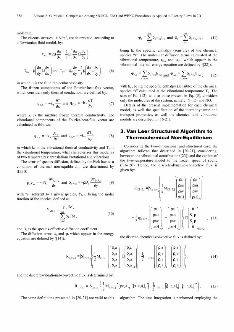
Figure 1. Contributions of Q− and Q+
to cell (i,j).
To k = 3, which implies a fifth-order WENO procedure, r
varies from 0 to 2. The values of crj and Q are shown in Tab.
362 Edisson S. G. Maciel: Comparison Among MUSCL, ENO and WENO Procedures as Applied to Reentry Flows in 2D
3:
Table 3. Values of r, crj and Q (5th Order).
R cr0 Q cr1 Q cr2 Q
0 1/3 iQ 5/6
i 1Q + -1/6 i 2Q +
1 -1/6 i 1Q − 5/6
iQ 1/3 i 1Q +
2 1/3 i 2Q − -7/6
i 1Q − 11/6 iQ
The values of dr, in Eq. (39) are: d0 = 3/10, d1 = 3/5, and d2 =
1/10. The expressions to the smooth indicators are:
( ) ( )2
2i1ii
2
2i1ii0 QQ4Q34
1QQ2Q
12
13++++ +−++−=β (41)
( ) ( )2
1i1i
2
1ii1i1 QQ4
1QQ2Q
12
13+−+− −++−=β ; (42)
( ) ( )2
i1i2i
2
i1i2i2 Q3Q4Q4
1QQ2Q
12
13 +−++−=β −−−− (43)
To Q+
, one has the values of rjc and Q , defined in Tab. 4.
The values of rd are given by: 0 2d d 1/10= = ,
1 1d d 3 / 5= = , and 2 0d d 3 /10= = . With the application of
Eq. (40), the rω coefficients are calculated and the Q−
and
Q+
functions are defined, Eqs. (37-38).
Table 4. Values of r, rjc and Q (5th Order).
r r0c Q r1c Q r 2c Q
0 11/6 iQ -7/6
i 1Q + 1/3 i 2Q +
1 1/3 i 1Q − 5/6
iQ -1/6 i 1Q +
2 -1/6 i 2Q − 5/6
i 1Q − 1/3 iQ
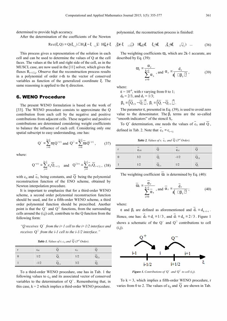
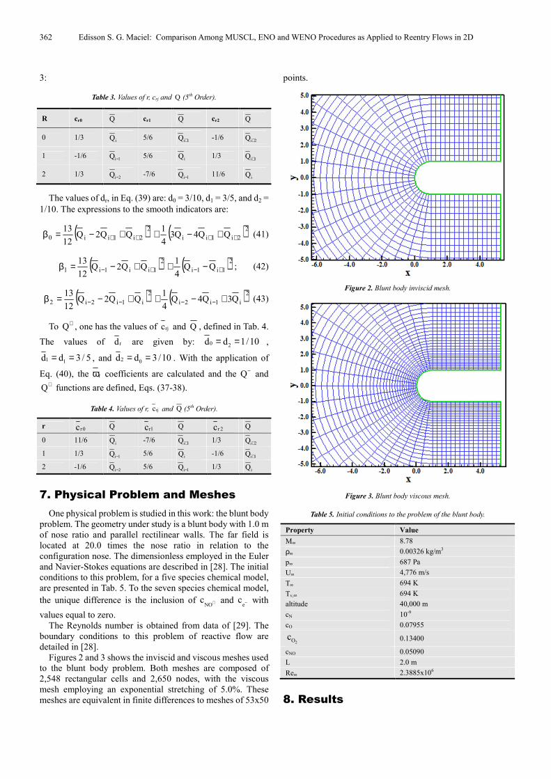
7. Physical Problem and Meshes
One physical problem is studied in this work: the blunt body
problem. The geometry under study is a blunt body with 1.0 m
of nose ratio and parallel rectilinear walls. The far field is
located at 20.0 times the nose ratio in relation to the
configuration nose. The dimensionless employed in the Euler
and Navier-Stokes equations are described in [28]. The initial
conditions to this problem, for a five species chemical model,
are presented in Tab. 5. To the seven species chemical model,
the unique difference is the inclusion of NO
c + and e
c − with
values equal to zero.
The Reynolds number is obtained from data of [29]. The
boundary conditions to this problem of reactive flow are
detailed in [28].
Figures 2 and 3 shows the inviscid and viscous meshes used
to the blunt body problem. Both meshes are composed of
2,548 rectangular cells and 2,650 nodes, with the viscous
mesh employing an exponential stretching of 5.0%. These
meshes are equivalent in finite differences to meshes of 53x50
points.
Figure 2. Blunt body inviscid mesh.
Figure 3. Blunt body viscous mesh.
Table 5. Initial conditions to the problem of the blunt body.
Property Value
M∞ 8.78
ρ∞ 0.00326 kg/m3
p∞ 687 Pa
U∞ 4,776 m/s
T∞ 694 K
Tv,∞ 694 K
altitude 40,000 m
cN 10-9
cO 0.07955
2Oc 0.13400
cNO 0.05090
L 2.0 m
Re∞ 2.3885x10⁶
8. Results

Computational and Applied Mathematics Journal 2015; 1(5): 355-377 363
Tests were performed in a notebook with Intel Processor
Core i7 and 6.0 GBytes of RAM, in a Windows 8.0
environment. As the interest of this work is steady state
problems, it is necessary to define a criterion which guarantees
the convergence of the numerical results. The criterion
adopted was to consider a reduction of no minimal three (3)
orders of magnitude in the value of the maximum residual in
the calculation domain, a typical CFD-community criterion.
The residual of each cell was defined as the numerical value
obtained from the discretized conservation equations. As there
are a maximum of eleven (11), seven species model,
conservation equations to each cell, the maximum value
obtained from these equations is defined as the residual of this
cell. Hence, this residual is compared with the residual of the
other cells, calculated of the same way, to define the maximum
residual in the calculation domain. In the simulations, the
attack angle was set equal to zero.
8.1. Blunt Body Problem
Chemical Non-Equilibrium. In this case, only the five
species model is analyzed. It is important to remember that in
this formulation, the vibrational contribution is not taken into
account. There is only a unique temperature field, that is, the
translational temperature. It is also important to remember that
in this formulation the diffusion transport mechanism present
in the viscous equations is not considered.
(a) Inviscid results:
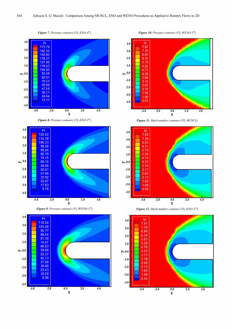
Figures 4 to 10 show pressure contours obtained by the 2nd
order MUSC result, the ENO results to 2nd
, 3rd
, 4th
and 5th
orders, and the WENO results to 3rd
and 5th orders. As can be
seen, good qualitative results are obtained by the three
procedures. In quantitative terms, there are different
estimations of the stagnation pressure.
Figure 4. Pressure contours (VL-MUSCL).
The MUSCL result estimates the stagnation pressure equal
to 120.69 unities, whereas the ENO results estimate the
stagnation pressure close to 172.00 (an average value among
the different values). On the other hand, the WENO results
estimate values to the stagnation pressure around 115.00
unities. All solutions present good symmetry properties.
Figure 5. Pressure contours (VL-ENO-2nd).
Figure 6. Pressure contours (VL-ENO-3rd).
364 Edisson S. G. Maciel: Comparison Among MUSCL, ENO and WENO Procedures as Applied to Reentry Flows in 2D
Figure 7. Pressure contours (VL-ENO-4th).
Figure 8. Pressure contours (VL-ENO-5th).
Figure 9. Pressure contours (VL-WENO-3rd).
Figure 10. Pressure contours (VL-WENO-5th).
Figure 11. Mach number contours (VL-MUSCL).
Figure 12. Mach number contours (VL-ENO-2nd).

Computational and Applied Mathematics Journal 2015; 1(5): 355-377 365
Figure 13. Mach number contours (VL-ENO-3rd).
Figure 14. Mach number contours (VL-ENO-4th).
Figure 15. Mach number contours (VL-ENO-5th).
Figure 16. Mach number contours (VL-WENO-3rd).
Figure 17. Mach number contours (VL-WENO-5th).
Figures 11 to 17 exhibit the Mach number contours
obtained by the three procedures. The ENO results present
more severe Mach number contours than the others. However,
the qualitative aspects of the ENO results show less
symmetrical contours in relation to the y = 0 axis than the
MUSCL and the WENO results. Moreover, the WENO results
present excellent symmetry properties altogether with the
MUSCL result. No pre-shock oscillations are present in the
seven figures; in other words, the Gibbs phenomenon was not
perceptible.
(b) Viscous results:
Figures 18 to 21 exhibit the pressure contours obtained by
the MUSC procedure, the 3rd
and 4th
order pressure contours
of the ENO procedure, and the 3rd
order pressure contours of
the WENO procedure. The second- and fifth-order results of
the ENO procedure did not converge, as well the fifth-order
results of the WENO procedure. Again higher stagnation
pressure values are observed in the ENO solutions than in the
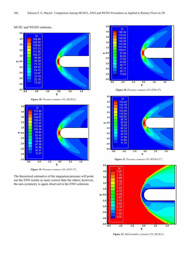
366 Edisson S. G. Maciel: Comparison Among MUSCL, ENO and WENO Procedures as Applied to Reentry Flows in 2D
MUSC and WENO solutions.
Figure 18. Pressure contours (VL-MUSCL).
Figure 19. Pressure contours (VL-ENO-3rd).
The theoretical estimative of the stagnation pressure will point
out the ENO results as more correct than the others; however,
the non-symmetry is again observed in the ENO solutions.
Figure 20. Pressure contours (VL-ENO-4th).
Figure 21. Pressure contours (VL-WENO-3rd).
Figure 22. Mach number contours (VL-MUSCL).

Computational and Applied Mathematics Journal 2015; 1(5): 355-377 367
Figure 23. Mach number contours (VL-ENO-3rd).
Figure 24. Mach number contours (VL-ENO-4th).
Figure 25. Mach number contours (VL-WENO-3rd).
Figures 22 to 25 present the Mach number contours
obtained by the MUSCL, by the ENO and by the WENO
procedures. Mach number fields more severe are observed in
the ENO results, although the 4th
order ENO and the 3rd
order
WENO results highlight a pre-shock oscillation. It is
important to emphasize that the suppression of pre-shock
oscillations is expected to surge effect only in the inviscid
results, where the convective contribution is appropriately
described by the Newton interpolation.
Thermochemical Non-Equilibrium. In this case, the five and
seven species models are analyzed. Moreover, the rotational,
and vibrational modes are considered in the Navier-Stokes
equation, as also the diffusivity contribution. Two
characteristic temperature fields are computed in these
formulations.
(a) Five species – Inviscid results:
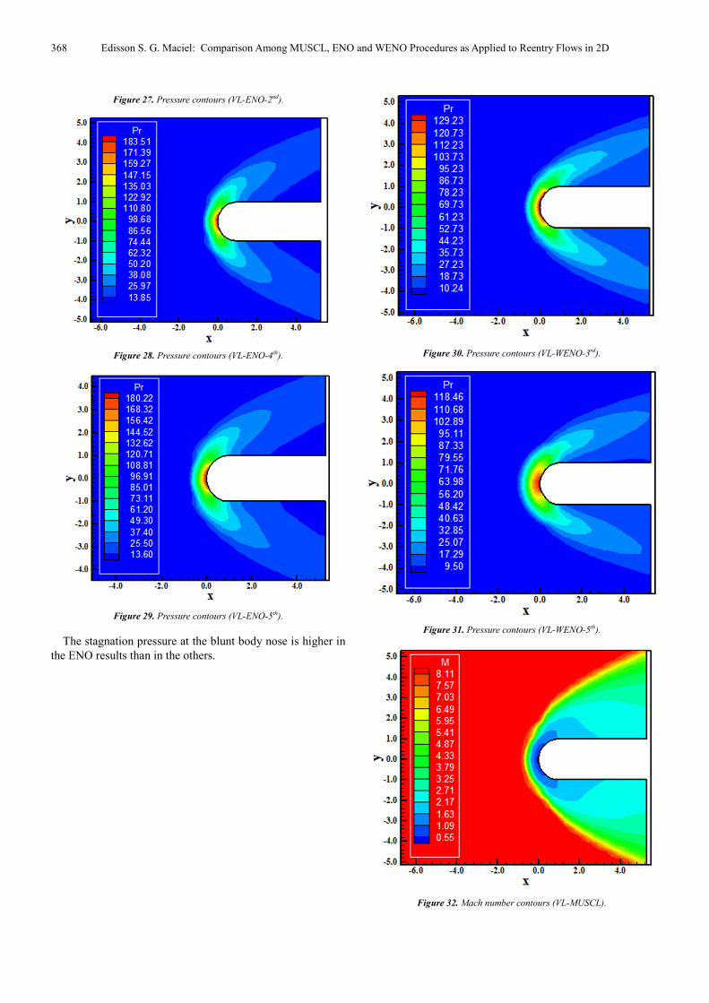
Figures 26 to 31 show the pressure contours obtained by the
MUSCL procedure, by the 2nd
, 4th
and 5th
order ENO
procedure, and by the 3rd
and 5th
order WENO procedure,
respectively. The 3rd
order ENO result did not converge to the
minimum considered criterion and was not plotted.
Figure 26. Pressure contours (VL-MUSCL).
368 Edisson S. G. Maciel: Comparison Among MUSCL, ENO and WENO Procedures as Applied to Reentry Flows in 2D
Figure 27. Pressure contours (VL-ENO-2nd).
Figure 28. Pressure contours (VL-ENO-4th).
Figure 29. Pressure contours (VL-ENO-5th).
The stagnation pressure at the blunt body nose is higher in
the ENO results than in the others.
Figure 30. Pressure contours (VL-WENO-3rd).
Figure 31. Pressure contours (VL-WENO-5th).
Figure 32. Mach number contours (VL-MUSCL).
Computational and Applied Mathematics Journal 2015; 1(5): 355-377 369
Figure 33. Mach number contours (VL-ENO-2nd).
Figure 34. Mach number contours (VL-ENO-4th).
Figure 35. Mach number contours (VL-ENO-5th).
Figure 36. Mach number contours (VL-WENO-3rd).
Figure 37. Mach number contours (VL-WENO-5th).
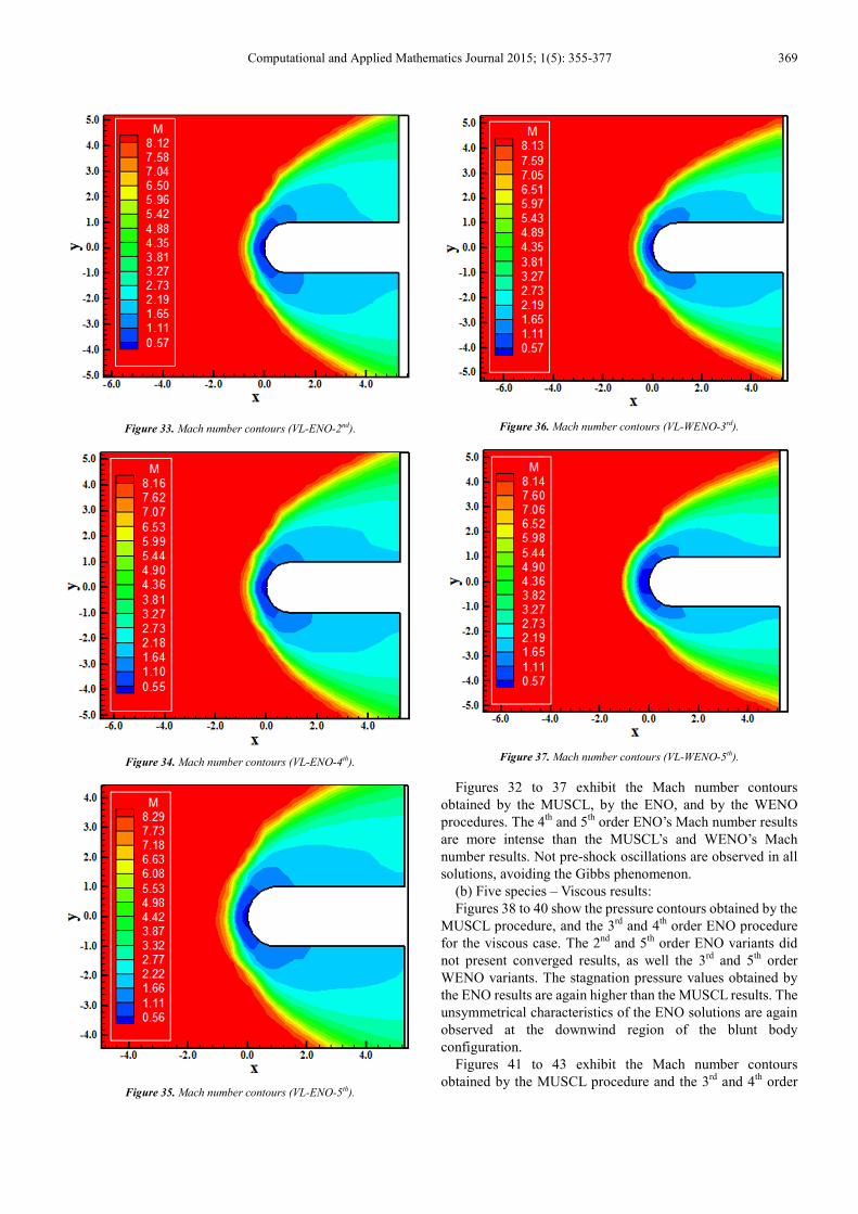
Figures 32 to 37 exhibit the Mach number contours
obtained by the MUSCL, by the ENO, and by the WENO
procedures. The 4th
and 5th
order ENO’s Mach number results
are more intense than the MUSCL’s and WENO’s Mach
number results. Not pre-shock oscillations are observed in all
solutions, avoiding the Gibbs phenomenon.
(b) Five species – Viscous results:
Figures 38 to 40 show the pressure contours obtained by the
MUSCL procedure, and the 3rd
and 4th
order ENO procedure
for the viscous case. The 2nd
and 5th
order ENO variants did
not present converged results, as well the 3rd
and 5th
order
WENO variants. The stagnation pressure values obtained by
the ENO results are again higher than the MUSCL results. The
unsymmetrical characteristics of the ENO solutions are again
observed at the downwind region of the blunt body
configuration.
Figures 41 to 43 exhibit the Mach number contours
obtained by the MUSCL procedure and the 3rd
and 4th
order
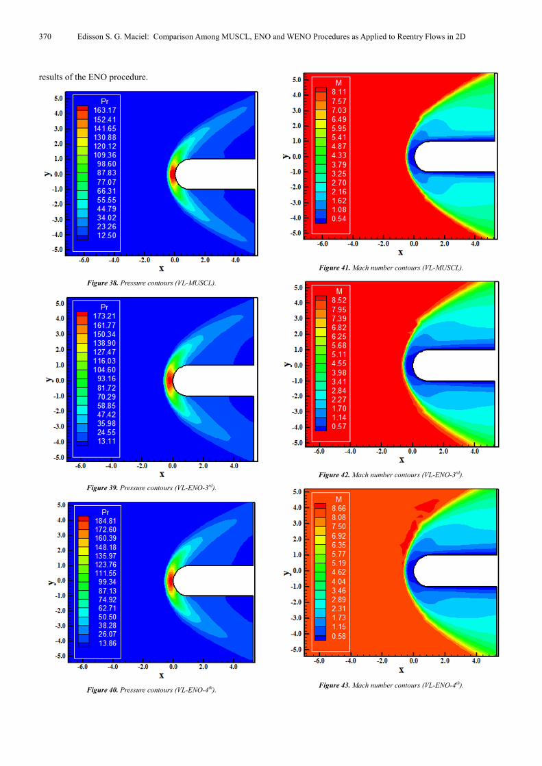
370 Edisson S. G. Maciel: Comparison Among MUSCL, ENO and WENO Procedures as Applied to Reentry Flows in 2D
results of the ENO procedure.
Figure 38. Pressure contours (VL-MUSCL).
Figure 39. Pressure contours (VL-ENO-3rd).
Figure 40. Pressure contours (VL-ENO-4th).
Figure 41. Mach number contours (VL-MUSCL).
Figure 42. Mach number contours (VL-ENO-3rd).
Figure 43. Mach number contours (VL-ENO-4th).
Computational and Applied Mathematics Journal 2015; 1(5): 355-377 371
Both ENO results present Mach number fields more intense
than the MUSCL result, although pre-shock oscillations are
observed in the 4th
order ENO result. It seems that the
limitation of the divided differences of the Newton
polynomial interpolation is not sufficient to avoid the Gibbs
phenomenon in the even variant.
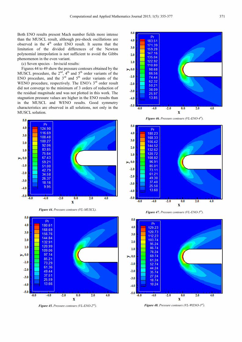
(c) Seven species – Inviscid results:
Figures 44 to 49 show the pressure contours obtained by the
MUSCL procedure, the 2nd
, 4th
and 5th
order variants of the
ENO procedure, and the 3rd
and 5th
order variants of the
WENO procedure, respectively. The ENO’s 3rd
order result
did not converge to the minimum of 3 orders of reduction of
the residual magnitude and was not plotted in this work. The
stagnation pressure values are higher in the ENO results than
in the MUSCL and WENO results. Good symmetry
characteristics are observed in all solutions, not only in the
MUSCL solution.
Figure 44. Pressure contours (VL-MUSCL).
Figure 45. Pressure contours (VL-ENO-2nd).
Figure 46. Pressure contours (VL-ENO-4th).
Figure 47. Pressure contours (VL-ENO-5th).
Figure 48. Pressure contours (VL-WENO-3rd).

372 Edisson S. G. Maciel: Comparison Among MUSCL, ENO and WENO Procedures as Applied to Reentry Flows in 2D
Figure 49. Pressure contours (VL-WENO-5th).
Figure 50. Mach number contours (VL-MUSCL).
Figure 51. Mach number contours (VL-ENO-2nd).
Figure 52. Mach number contours (VL-ENO-4th).
Figure 53. Mach number contours (VL-ENO-5th).
Figure 54. Mach number contours (VL-WENO-3rd).
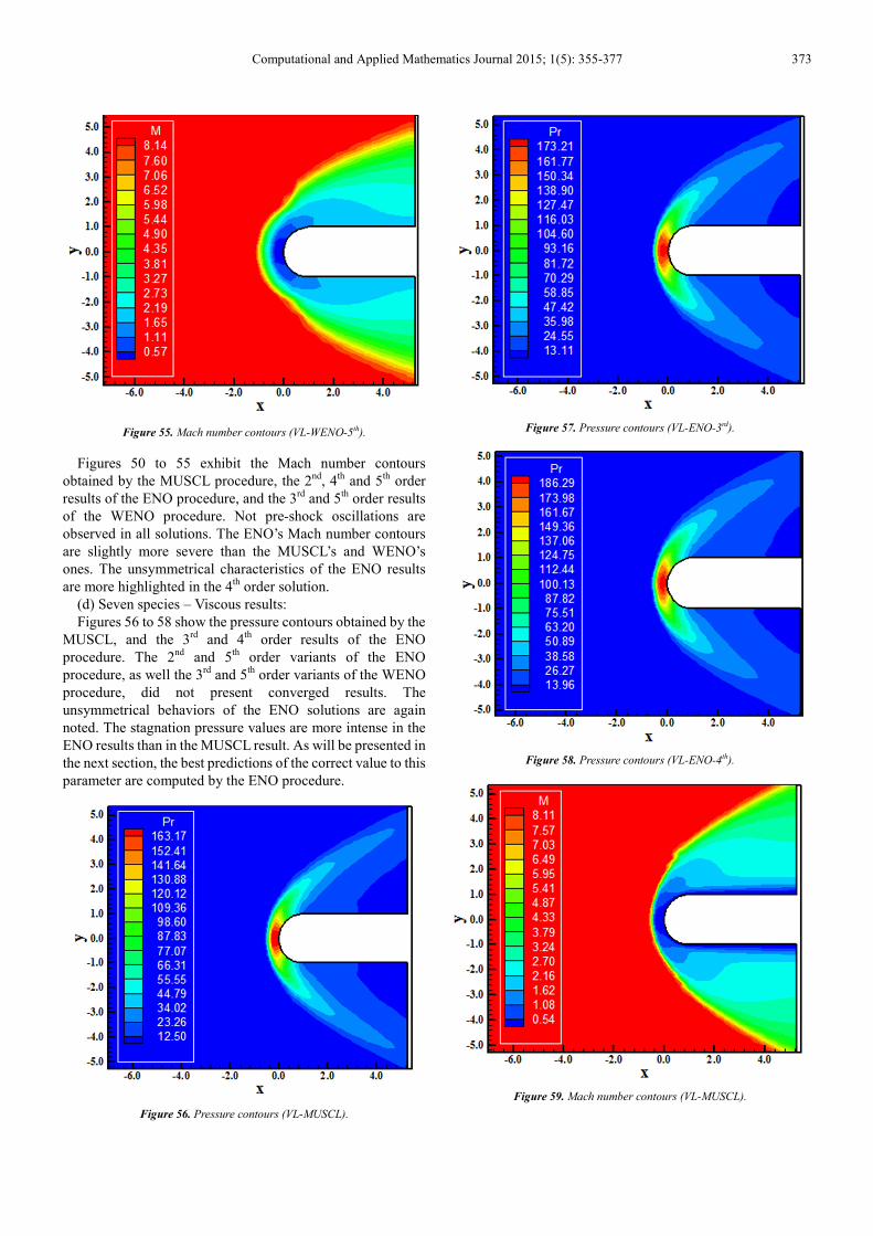
Computational and Applied Mathematics Journal 2015; 1(5): 355-377 373
Figure 55. Mach number contours (VL-WENO-5th).
Figures 50 to 55 exhibit the Mach number contours
obtained by the MUSCL procedure, the 2nd
, 4th
and 5th
order
results of the ENO procedure, and the 3rd
and 5th
order results
of the WENO procedure. Not pre-shock oscillations are
observed in all solutions. The ENO’s Mach number contours
are slightly more severe than the MUSCL’s and WENO’s
ones. The unsymmetrical characteristics of the ENO results
are more highlighted in the 4th
order solution.
(d) Seven species – Viscous results:
Figures 56 to 58 show the pressure contours obtained by the
MUSCL, and the 3rd
and 4th
order results of the ENO
procedure. The 2nd
and 5th order variants of the ENO
procedure, as well the 3rd
and 5th
order variants of the WENO
procedure, did not present converged results. The
unsymmetrical behaviors of the ENO solutions are again
noted. The stagnation pressure values are more intense in the
ENO results than in the MUSCL result. As will be presented in
the next section, the best predictions of the correct value to this
parameter are computed by the ENO procedure.
Figure 56. Pressure contours (VL-MUSCL).
Figure 57. Pressure contours (VL-ENO-3rd).
Figure 58. Pressure contours (VL-ENO-4th).
Figure 59. Mach number contours (VL-MUSCL).
374 Edisson S. G. Maciel: Comparison Among MUSCL, ENO and WENO Procedures as Applied to Reentry Flows in 2D
Figure 60. Mach number contours (VL-ENO-3rd).
Figure 61. Mach number contours (VL-ENO-4th).
Figures 59 to 61 exhibit the Mach number contours
obtained by the MUSCL procedure, and by the ENO 3rd and
4th order variants. The ENO’s Mach number contours are
more intense than the MUSCL’s ones. Pre-shock oscillations
are observed in the 4th order ENO results. As aforementioned,
the best ENO behavior is expected to the inviscid case, not to
the viscous case, although the MUSCL solution did not
indicate such behavior.
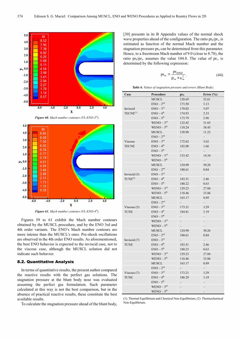
8.2. Quantitative Analysis
In terms of quantitative results, the present author compared
the reactive results with the perfect gas solutions. The
stagnation pressure at the blunt body nose was evaluated
assuming the perfect gas formulation. Such parameter
calculated at this way is not the best comparison, but in the
absence of practical reactive results, these constitute the best
available results.
To calculate the stagnation pressure ahead of the blunt body,
[30] presents in its B Appendix values of the normal shock
wave properties ahead of the configuration. The ratio pr0/pr∞ is
estimated as function of the normal Mach number and the
stagnation pressure pr0 can be determined from this parameter.
Hence, to a freestream Mach number of 9.0 (close to 8.78), the
ratio pr0/pr∞ assumes the value 104.8. The value of pr∞ is
determined by the following expression:
2
initial
a
prpr
∞∞∞
×ρ= . (44)
Table 6. Values of stagnation pressure and errors (Blunt Body).
Case Procedure pr0 Error (%)
MUSCL 120.69 32.61
ENO – 2nd 173.50 3.13
Inviscid ENO – 3rd 170.02 5.07
TECNE(1) ENO – 4th 174.93 2.33
ENO – 5th 173.79 2.96
WENO – 3rd 122.42 31.65
WENO – 5th 110.24 38.45
MUSCL 158.98 11.23
ENO – 2nd – –
Viscous ENO – 3rd 172.62 3.62
TECNE ENO – 4th 182.08 1.66
ENO – 5th – –
WENO – 3rd 153.42 14.34
WENO – 5th – –
MUSCL 124.90 30.26
ENO – 2nd 180.61 0.84
Inviscid (5) ENO – 3rd – –
TCNE(2) ENO – 4th 183.51 2.46
ENO – 5th 180.22 0.63
WENO – 3rd 129.23 27.84
WENO – 5th 118.46 33.86
MUSCL 163.17 8.89
ENO – 2nd – –
Viscous (5) ENO – 3rd 173.21 3.29
TCNE ENO – 4th 184.81 3.19
ENO – 5th – –
WENO – 3rd – –
WENO – 5th – –
MUSCL 124.90 30.26
ENO – 2nd 180.61 0.84
Inviscid (7) ENO – 3rd – –
TCNE ENO – 4th 183.51 2.46
ENO – 5th 180.23 0.63
WENO – 3rd 129.23 27.84
WENO – 5th 118.46 33.86
MUSCL 163.17 8.89
ENO – 2nd – –
Viscous (7) ENO – 3rd 173.21 3.29
TCNE ENO – 4th 186.29 3.19
ENO – 5th – –
WENO – 3rd – –
WENO – 5th – –
(1): Thermal Equilibrium and Chemical Non-Equilibrium; (2): Thermochemical
Non-Equilibrium.

Computational and Applied Mathematics Journal 2015; 1(5): 355-377 375
In the present study, prinitial = 687N/m2, ρ∞ = 0.004kg/m
3 and
a∞ = 317.024m/s. Considering these values, one concludes that
pr∞ = 1.709 (non-dimensional). Using the ratio obtained from
[30], the stagnation pressure ahead of the configuration nose is
estimated as 179.10 unities. Table 6 compares the values
obtained from the simulations with this theoretical parameter
and presents the numerical percentage errors. As can be
observed, all ENO’s solutions present percentage errors less
than 5.10%, which is an excellent estimation of the stagnation
pressure.
Table 7. Values of the shock standoff distance (Blunt Body).
Case Procedure δδδδNUM (m) Error (%)
MUSCL 0.40 5.26
ENO – 2nd 0.40 5.26
Inviscid ENO – 3rd 0.41 7.89
TECNE ENO – 4th 0.41 7.89
ENO – 5th 0.46 21.05
WENO – 3rd 0.45 18.42
WENO – 5th 0.65 71.05
MUSCL 0.35 7.89
ENO – 2nd – –
Viscous ENO – 3rd 0.30 21.05
TECNE ENO – 4th 0.31 18.42
ENO – 5th – –
WENO – 3rd 0.31 18.42
WENO – 5th – –
MUSCL 0.37 2.63
ENO – 2nd 0.37 2.63
Inviscid (5) ENO – 3rd – –
TCNE ENO – 4th 0.38 0.00
ENO – 5th 0.41 7.89
WENO – 3rd 0.38 0.00
WENO – 5th 0.50 31.58
MUSCL 0.30 21.05
ENO – 2nd – –
Viscous (5) ENO – 3rd 0.32 15.79
TCNE ENO – 4th 0.31 18.42
ENO – 5th – –
WENO – 3rd – –
WENO – 5th – –
MUSCL 0.39 2.63
ENO – 2nd 0.38 0.00
Inviscid (7) ENO – 3rd – –
TCNE ENO – 4th 0.37 2.63
ENO – 5th 0.38 0.00
WENO – 3rd 0.39 2.63
WENO – 5th 0.52 36.84
MUSCL 0.30 21.05
ENO – 2nd – –
Viscous (7) ENO – 3rd 0.31 18.42
TCNE ENO – 4th 0.31 18.42
ENO – 5th – –
WENO – 3rd – –
WENO – 5th – –
The best results were obtained with the ENO 5th
order, in an
inviscid case, as expected, and using a five (5) and seven (7)
species thermochemical non-equilibrium formulation, with an
error of 0.63%.
An important observation with the studied problem in this
work is that more realistic results were obtained with the more
complete formulation of thermochemical non-equilibrium, as
expected. The thermochemical non-equilibrium formulation,
using five (5) and seven (7) species, constitutes a good tool to
describe the translational/rotational and vibrational modes of
excitation.
The expectative is that with more severe conditions, the
seven (7) species model be better than the five (5) species
model because the former consider the ionization process
typical of more elaborated flow conditions. Moreover, the
eleven (11) species model should be the most realistic version
of this algorithm, in both simplified and full versions.
Another possibility to quantify the results is the
determination of the shock standoff distance. [34] presents a
graphic in which is plotted the shock standoff distance of a
pre-determined configuration versus the Mach number.
Considering the blunt body nose approximately as a cylinder
and using the value 8.78 to the Mach number, it is possible to
obtain the value 0.19 to the ratio δ/d, where δ is the position of
the normal shock wave in relation to the body nose and d is a
configuration characteristic length. In the present study, d =
2.0m (diameter of the body nose) and δ = 0.38m. Table 7
presents the values obtained by δ for the different cases and
the percentage errors. This table shows that the best results are
obtained with the inviscid 4th
order variant of the ENO
procedure and with the inviscid 3rd
order variant of the WENO
procedure, with errors of 0.00%, respectively, as using the five
(5) and seven (7) species formulations.
As the shock standoff distance presented in [34] is more
realistic, presenting smaller dependence of the perfect gas
hypothesis, improved results were expected to be obtained in
the present study.
8.3. Computational Performance
Table 8 presents the computational data of the MUSCL,
ENO and WENO simulations for the blunt body problem. It
shows the CFL number and the number of iterations to
convergence for all studied cases in the present work. As can
be seen, the best performances are due to the MUSCL
procedure, where CFL numbers of 0.10 were always used.
With it, convergences in less than 4,500 iterations were
always obtained. The best ENO performance was due to the
5th order variant, in the chemical non-equilibrium formulation
and inviscid case, with CFL number of 0.10 and convergence
in 2,518 iterations. On the other hand, the WENO 5th order
variant converged in 1,383 iterations, in the chemical
non-equilibrium inviscid case, and was the absolute best
behavior considering all variants.
Although the best performances indicate the MUSCL
approach as better than the ENO and WENO approaches, the
best behavior of the ENO approach in terms of quantitative
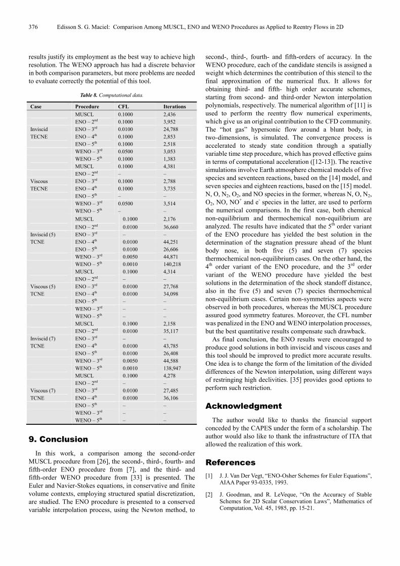
376 Edisson S. G. Maciel: Comparison Among MUSCL, ENO and WENO Procedures as Applied to Reentry Flows in 2D
results justify its employment as the best way to achieve high
resolution. The WENO approach has had a discrete behavior
in both comparison parameters, but more problems are needed
to evaluate correctly the potential of this tool.
Table 8. Computational data.
Case Procedure CFL Iterations
MUSCL 0.1000 2,436
ENO – 2nd 0.1000 3,952
Inviscid ENO – 3rd 0.0100 24,788
TECNE ENO – 4th 0.1000 2,853
ENO – 5th 0.1000 2,518
WENO – 3rd 0.0500 3,053
WENO – 5th 0.1000 1,383
MUSCL 0.1000 4,381
ENO – 2nd – –
Viscous ENO – 3rd 0.1000 2,788
TECNE ENO – 4th 0.1000 3,735
ENO – 5th – –
WENO – 3rd 0.0500 3,514
WENO – 5th – –
MUSCL 0.1000 2,176
ENO – 2nd 0.0100 36,660
Inviscid (5) ENO – 3rd – –
TCNE ENO – 4th 0.0100 44,251
ENO – 5th 0.0100 26,606
WENO – 3rd 0.0050 44,871
WENO – 5th 0.0010 140,218
MUSCL 0.1000 4,314
ENO – 2nd – –
Viscous (5) ENO – 3rd 0.0100 27,768
TCNE ENO – 4th 0.0100 34,098
ENO – 5th – –
WENO – 3rd – –
WENO – 5th – –
MUSCL 0.1000 2,158
ENO – 2nd 0.0100 35,117
Inviscid (7) ENO – 3rd – –
TCNE ENO – 4th 0.0100 43,785
ENO – 5th 0.0100 26,408
WENO – 3rd 0.0050 44,588
WENO – 5th 0.0010 138,947
MUSCL 0.1000 4,278
ENO – 2nd – –
Viscous (7) ENO – 3rd 0.0100 27,485
TCNE ENO – 4th 0.0100 36,106
ENO – 5th – –
WENO – 3rd – –
WENO – 5th – –
9. Conclusion
In this work, a comparison among the second-order
MUSCL procedure from [26], the second-, third-, fourth- and
fifth-order ENO procedure from [7], and the third- and
fifth-order WENO procedure from [33] is presented. The
Euler and Navier-Stokes equations, in conservative and finite
volume contexts, employing structured spatial discretization,
are studied. The ENO procedure is presented to a conserved
variable interpolation process, using the Newton method, to
second-, third-, fourth- and fifth-orders of accuracy. In the
WENO procedure, each of the candidate stencils is assigned a
weight which determines the contribution of this stencil to the
final approximation of the numerical flux. It allows for
obtaining third- and fifth- high order accurate schemes,
starting from second- and third-order Newton interpolation
polynomials, respectively. The numerical algorithm of [11] is
used to perform the reentry flow numerical experiments,
which give us an original contribution to the CFD community.
The “hot gas” hypersonic flow around a blunt body, in
two-dimensions, is simulated. The convergence process is
accelerated to steady state condition through a spatially
variable time step procedure, which has proved effective gains
in terms of computational acceleration ([12-13]). The reactive
simulations involve Earth atmosphere chemical models of five
species and seventeen reactions, based on the [14] model, and
seven species and eighteen reactions, based on the [15] model.
N, O, N2, O2, and NO species in the former, whereas N, O, N2,
O2, NO, NO+ and e
- species in the latter, are used to perform
the numerical comparisons. In the first case, both chemical
non-equilibrium and thermochemical non-equilibrium are
analyzed. The results have indicated that the 5th
order variant
of the ENO procedure has yielded the best solution in the
determination of the stagnation pressure ahead of the blunt
body nose, in both five (5) and seven (7) species
thermochemical non-equilibrium cases. On the other hand, the
4th
order variant of the ENO procedure, and the 3rd
order
variant of the WENO procedure have yielded the best
solutions in the determination of the shock standoff distance,
also in the five (5) and seven (7) species thermochemical
non-equilibrium cases. Certain non-symmetries aspects were
observed in both procedures, whereas the MUSCL procedure
assured good symmetry features. Moreover, the CFL number
was penalized in the ENO and WENO interpolation processes,
but the best quantitative results compensate such drawback.
As final conclusion, the ENO results were encouraged to
produce good solutions in both inviscid and viscous cases and
this tool should be improved to predict more accurate results.
One idea is to change the form of the limitation of the divided
differences of the Newton interpolation, using different ways
of restringing high declivities. [35] provides good options to
perform such restriction.
Acknowledgment
The author would like to thanks the financial support
conceded by the CAPES under the form of a scholarship. The
author would also like to thank the infrastructure of ITA that
allowed the realization of this work.
References
[1] J. J. Van Der Vegt, “ENO-Osher Schemes for Euler Equations”, AIAA Paper 93-0335, 1993.
[2] J. Goodman, and R. LeVeque, “On the Accuracy of Stable Schemes for 2D Scalar Conservation Laws”, Mathematics of Computation, Vol. 45, 1985, pp. 15-21.
Computational and Applied Mathematics Journal 2015; 1(5): 355-377 377
[3] S. Osher, and S. R. Chakravarthy, “High Resolution Schemes and the Entropy Condition”, SIAM Journal on Numerical Analysis, Vol. 21, 1984, pp. 955-984.
[4] C. Hirsch, “Numerical Computation of Internal and External Flows Computational Methods for Inviscid and Viscous Flows”, John Wiley & Sons Ltd, 691p., 1990.
[5] A. Harten, S. Osher, B. Engquist, S. R. Chakravarthy, “Some Results on Uniformly High Order Accurate Essentially Non-Oscillatory Schemes”, Journal of Applied Numerical Mathematics, Vol. 2, 1986, pp. 347-377.
[6] A. Harten, and S. Osher, “Uniformly High-Order Accurate Nonoscillatory Schemes I”, SIAM Journal on Numerical Analysis, Vol. 24, 1987, pp. 279-309.
[7] A. Harten, B. Engquist, S. Osher, S. R. Chakravarthy, “Uniformly High Order Accurate Essentially Non-Oscillatory Schemes III”, Journal of Computational Physics, Vol. 71, 1987, pp. 231-303.
[8] A. Harten, and S. R. Chakravarthy, “Multi-Dimensional ENO Schemes for General Geometries”, ICASE Report 91-76, NASA Langley, Virginia, 1991.
[9] C. –W. Shu, and S. Osher, “Efficient Implementation of Essentially Non-Oscillatory Shock-Capturing Schemes”, Journal of Computational Physics, Vol. 77, 1988, pp. 439-471.
[10] C. –W. Shu, and S. Osher, “Efficient Implementation of Essentially Non-Oscillatory Shock Capturing Schemes, II”, Journal of Computational Physics, Vol. 83, 1989, pp. 32-78.
[11] B. Van Leer, “Flux-Vector Splitting for the Euler Equations”, Lecture Notes in Physics, Springer Verlag, Berlin, Vol. 170, 1982, pp. 507-512.
[12] E. S. G. Maciel, Simulations in 2D and 3D Applying Unstructured Algorithms, Euler and Navier-Stokes Equations – Perfect Gas Formulation. Saarbrücken, Deutschland: Lambert Academic Publishing (LAP), 2015, Ch. 1, pp. 26-47.
[13] E. S. G. Maciel, Simulations in 2D and 3D Applying Unstructured Algorithms, Euler and Navier-Stokes Equations – Perfect Gas Formulation. Saarbrücken, Deutschland: Lambert Academic Publishing (LAP), 2015, Ch. 6, pp. 160-181.
[14] S. K. Saxena and M. T. Nair, “An Improved Roe Scheme for Real Gas Flow”, AIAA Paper 2005-587, 2005.
[15] F. G. Blottner, “Viscous Shock Layer at the Stagnation Point With Nonequilibrium Air Chemistry”, AIAA Journal, Vol. 7, No. 12, 1969, pp. 2281-2288.
[16] E. S. G. Maciel, and A. P. Pimenta, “Thermochemical Non-Equilibrium Reentry Flows in Two-Dimensions – Part I”, WSEAS Transactions on Mathematics, Vol. 11, Issue 6, 2012, pp. 520-545.
[17] E. S. G. Maciel, and A. P. Pimenta, “Thermochemical Non-Equilibrium Reentry Flows in Two-Dimensions – Part II”, WSEAS Transactions on Mathematics, Vol. 11, Issue 11, 2012, pp. 977-1005.
[18] E. S. G. Maciel, and A. P. Pimenta, “Thermochemical Non-Equilibrium Reentry Flows in Two-Dimensions: Seven Species Model – Part I”, WSEAS Transactions on Applied and Theoretical Mechanics, Vol. 7, Issue 4, 2012, pp. 311-337.
[19] E. S. G. Maciel, and A. P. Pimenta, “Thermochemical Non-Equilibrium Reentry Flows in Two-Dimensions: Seven Species Model – Part II”, WSEAS Transactions on Applied and Theoretical Mechanics, Vol. 8, Issue 1, 2013, pp. 55-83.
[20] E. S. G. Maciel, and A. P. Pimenta, “Chemical Non-Equilibrium Reentry Flows in Two-Dimensions – Part I”, WSEAS Transactions on Fluid Mechanics, Vol. 8, Issue 1, 2013, pp. 1-20.
[21] E. S. G. Maciel, and A. P. Pimenta, “Chemical Non-Equilibrium Reentry Flows in Two-Dimensions – Part II”, WSEAS Transactions on Fluid Mechanics, Vol. 8, Issue 2, 2013, pp. 50-79.
[22] R. K. Prabhu, “An Implementation of a Chemical and Thermal Nonequilibrium Flow Solver on Unstructured Meshes and Application to Blunt Bodies”, NASA CR-194967, 1994.
[23] D. Ait-Ali-Yahia, and W. G. Habashi, “Finite Element Adaptive Method for Hypersonic Thermochemical Nonequilibrium Flows”, AIAA Journal Vol. 35, No. 8, 1997, 1294-1302.
[24] R. Radespiel, and N. Kroll, “Accurate Flux Vector Splitting for Shocks and Shear Layers”, Journal of Computational Physics, Vol. 121, 1995, pp. 66-78.
[25] L. N. Long, M. M. S. Khan, and H. T. Sharp, “Massively Parallel Three-Dimensional Euler / Navier-Stokes Method”, AIAA Journal, Vol. 29, No. 5, 1991, pp. 657-666.
[26] B. Van Leer, “Towards the Ultimate Conservative Difference Scheme. II. Monotonicity and Conservation Combined in a Second-Order Scheme”, Journal of Computational Physics, Vol. 14, 1974, pp. 361-370.
[27] P. L. Roe, In Proceedings of the AMS-SIAM “Summer Seminar on Large-Scale Computation in Fluid Mechanics”, Edited by B. E. Engquist et al, Lectures in Applied Mathematics, Vol. 22, 1983, p. 163.
[28] E. S. G., Maciel, “Relatório ao CNPq (Conselho Nacional de Desenvolvimento Científico e Tecnológico) sobre as atividades de pesquisa realizadas no período de 01/07/2009 até 31/12/2009 com relação ao projeto PDJ número 150143/2008-7”, Report to the National Council of Scientific and Technological Development (CNPq), São José dos Campos, SP, Brasil, 102p, 2009. [available in the website www.edissonsavio.eng.br]
[29] R. W. Fox, and A. T. McDonald, “Introdução à Mecânica dos Fluidos”, Guanabara Editor, 1988.
[30] J. D. Anderson Jr., “Fundamentals of Aerodynamics”, McGraw-Hill, Inc., 5th Edition, 1008p., 2010.
[31] G. –S. Jiang, and C. –W. Shu, “Efficient Implementation of Weighted ENO Schemes”, Journal of Computational Physics, Vol. 126, 1996, pp. 202-228.
[32] X. –D. Liu, S. Osher, and T. Chan, “Weighted Essentially Non-oscillatory Schemes”, Journal of Computational Physics, Vol. 115, 1994, pp. 200-212.
[33] C. –W. Shu, “Essentially Non-Oscillatory and Weighted Essentially Non-Oscillatory Schemes for Hyperbolic Conservation Laws”, ICASE Report No. 97-65, 1997.
[34] H. W. Liepmann, and A. Roshko, “Elements of Gasdynamics”, John Wiley & Sons, Inc., 1st Edition, 439p, 1957.

378 Edisson S. G. Maciel: Comparison Among MUSCL, ENO and WENO Procedures as Applied to Reentry Flows in 2D
[35] C. B. Laney, “Computational Gasdynamics”, Cambridge University Press, 1st Edition, 613p., 1998.