978-1-5386-7138-2/18/$31.00 ©2018 IEEE

Comparing the Impact of HEMP Electric Field Waveforms on a Synthetic Grid

Raymund Lee and Thomas J. Overbye Department of Electrical and Computer Engineering

Texas A&M University College Station, TX, USA

Email: lee32982@tamu.edu | overbye@tamu.edu

Abstract—A nuclear bomb detonated above the earth’s surface can cause a high altitude electromagnetic pulse (HEMP). HEMP’s create an electric field at the earth’s surface, which induces unwanted slowly varying dc currents on transmission lines. To evaluate a power grid’s vulnerability to HEMP’s, two electric field waveforms have been used, having peak electric fields of 24 volts per km and 40 volts per km. Recently, a report was released containing six time-varying electric field waveforms and justified using a peak electric field of 84.57 volts per km. This paper compares how the magnitude of each electric field waveform is affected by different 1D conductivity regions. In addition, the impact of each electric field on a 10,000-bus synthetic grid will be evaluated. Analysis of the new waveforms show that there is not a single worst-case waveform. Different electric field waveforms have characteristics that affect the grid in varying ways. It is recommended that comprehensive HEMP vulnerability studies be done with multiple waveforms.

Index Terms—High Altitude Electromagnetic Pulse (HEMP), Geomagnetically Induced Current (GIC), Vulnerability Analysis

I. INTRODUCTION

A high altitude electromagnetic pulse (HEMP) occurs when a nuclear bomb is detonated 30 kilometers (km) or more above the earth’s surface. The HEMP’s blast generates an electric field at the earth’s surface comprised of three consecutive components called E1, E2, and E3. The E1 and E2 components occur first and have durations measured in microseconds and magnitudes measured in hundreds to thousands of volts per km [1]. The E3 occurs last, having magnitudes on the order of tens of volts per km and a duration that can be measured in seconds. Because of these differences, each HEMP electric field component is studied differently. The scope of this paper only includes the E3 component.

The HEMP’s electric field induces slowly varying dc currents, called geomagnetically induced currents (GIC), on transmission lines. To calculate the GIC throughout the grid, the dc voltage induced on the transmission lines, Vdc, must be calculated first using (1) which integrates the electric field, E, along the incremental path of the line, . [2]

=∮ ∙ (1)

GIC imposes a dc-offset on the ac currents that normally flow throughout a power grid. When GIC flow through a transformer, its core saturates, leading to unwanted consequences such as the generation of harmonics, the absorption of reactive power, and transformer heating.

To evaluate the impact of a HEMP’s electric field on a power grid, two publicly available waveforms from [3] and [4] have been used [5]-[7]. Reference [3] and [4] describe electric fields with peak magnitudes of 24 and 40 volts per km respectively.

More recently, [8] was released which declared that the magnitudes of past HEMP electric field waveforms were too low and suggested using a peak electric field of 84.57 volts per km. Six new time-varying and spatially-varying electric fields were also described.

The goal of this paper is to compare the grid impacts of all the HEMP electric fields mentioned above. These waveforms will be applied to a 10,000-bus synthetic case [9], [10]. Their impact on voltage stability and the amount of GIC flowing through transformers will be evaluated.

The paper is organized as follows. Section II covers background information. Section III describes the techniques used in this paper to calculate HEMP electric fields and model their effects. Section IV illustrates how the six electric field waveforms vary under different conductivity regions. It also analyzes the impact of these waveforms on a synthetic grid. Section V summarizes the paper by highlighting key points.

II. BACKGROUND

A. 1D Conductivity Model

The magnitude of the HEMP electric field heavily depends on the earth’s conductivity, hundreds of kilometers beneath the surface. Equations (2) and (3) describe how the impedance of the earth, acts as a transfer function between the electric field and magnetic field.

( ) = ( ) ( ) (2)

( ) = ( ) ( ) (3) E electric field magnitude; Z surface impedance; B magnetic flux density; µ0 magnetic permeability of free space; x northern direction; y eastern direction; ω angular frequency;

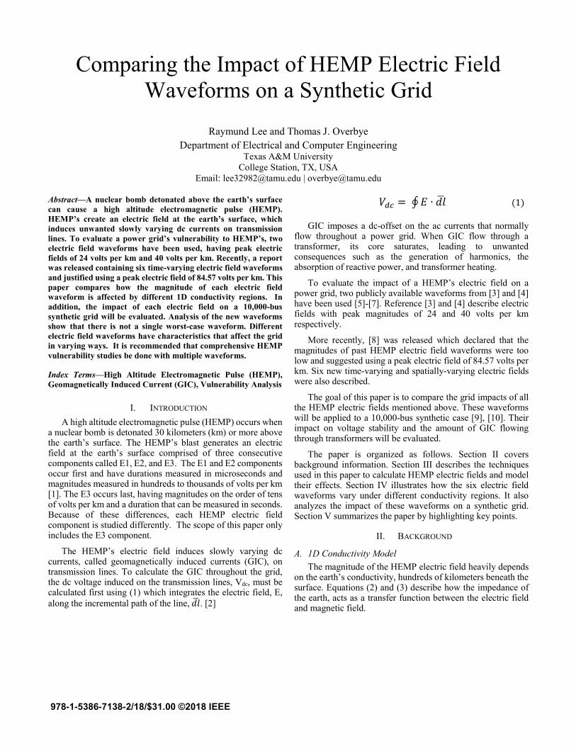
Different models are used to represent the earth’s conductivity. The electric fields from [3], [4], and [8] use uniform conductivity models which assume the earth has a single value of conductivity (10-3, 10-4, and 10-3 Siemens per meter, respectively). This paper utilizes a more detailed ground model called the 1D model from [11] which describes the earth in flat layers of varying thickness and conductivity levels, shown on Fig. 1.

Fig. 1. 1D conductivity model [13]

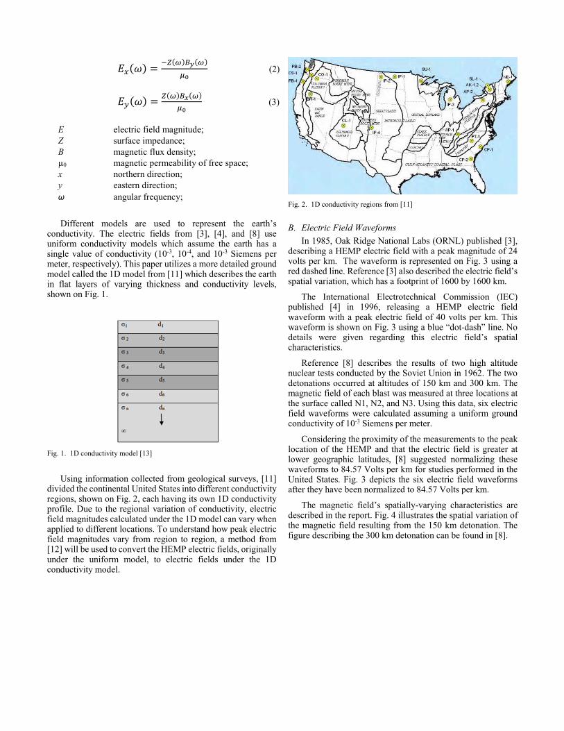
Using information collected from geological surveys, [11] divided the continental United States into different conductivity regions, shown on Fig. 2, each having its own 1D conductivity profile. Due to the regional variation of conductivity, electric field magnitudes calculated under the 1D model can vary when applied to different locations. To understand how peak electric field magnitudes vary from region to region, a method from [12] will be used to convert the HEMP electric fields, originally under the uniform model, to electric fields under the 1D conductivity model.

Fig. 2. 1D conductivity regions from [11]

B. Electric Field Waveforms

In 1985, Oak Ridge National Labs (ORNL) published [3], describing a HEMP electric field with a peak magnitude of 24 volts per km. The waveform is represented on Fig. 3 using a red dashed line. Reference [3] also described the electric field’s spatial variation, which has a footprint of 1600 by 1600 km.

The International Electrotechnical Commission (IEC) published [4] in 1996, releasing a HEMP electric field waveform with a peak electric field of 40 volts per km. This waveform is shown on Fig. 3 using a blue “dot-dash” line. No details were given regarding this electric field’s spatial characteristics.

Reference [8] describes the results of two high altitude nuclear tests conducted by the Soviet Union in 1962. The two detonations occurred at altitudes of 150 km and 300 km. The magnetic field of each blast was measured at three locations at the surface called N1, N2, and N3. Using this data, six electric field waveforms were calculated assuming a uniform ground conductivity of 10-3 Siemens per meter.

Considering the proximity of the measurements to the peak location of the HEMP and that the electric field is greater at lower geographic latitudes, [8] suggested normalizing these waveforms to 84.57 Volts per km for studies performed in the United States. Fig. 3 depicts the six electric field waveforms after they have been normalized to 84.57 Volts per km.

The magnetic field’s spatially-varying characteristics are described in the report. Fig. 4 illustrates the spatial variation of the magnetic field resulting from the 150 km detonation. The figure describing the 300 km detonation can be found in [8].

Fig. 3. Plot of newly-released electric field waveforms, the ORNL 1985 waveform, and the IEC 1996 waveform

Fig. 4. Spatial variation of magnetic field magnitude and direction as shown in [8]. N1, N2, and N3 are the measurement locations.

III. METHODOLOGY

This section covers how the electric field waveforms described in Fig. 3 and Fig. 4 were manipulated to obtain spatially-varying and time-varying electric fields under the 1D model. It also describes how their impact on the grid is modeled.

A. Obtaining Electric Field Under the 1D Model

As mentioned earlier, the electric field waveforms were published assuming the earth has a uniform conductivity. To apply the 1D model to these electric fields, they must first be converted back to a magnetic field using (2) and (3) [12], [13]. To obtain Z(ω), (4) is used, where σ is the uniform conductivity value. E(ω) is obtained by taking an FFT of one of the time-varying electric field waveforms in Fig. 3.

( ) = (4)

Once B(ω) is obtained, it can be combined with Fig. 4 to obtain a spatially-varying and time-varying magnetic field, Bx(x,y,ω) and By(x,y,ω). Equations (2) and (3) can be invoked again, but this time, to calculate the electric field under the 1D model. To find Z(ω) for the 1D model, an iterative method from [13] is used. It is important to note that the 1D region may differ at each point on the spatial grid. After obtaining Ex(x,y,ω) and Ey(x,y,ω), an inverse FFT can be performed to bring the electric field back to the time domain.

B. Modeling the Impact of HEMP’s

Once the electric field has been converted under the 1D model in the time domain, (1) can be used to determine the induced dc voltage on transmission lines.

Next, dc bus voltages, V, can be calculated using (5). G is the network conductance matrix which is augmented to include substation grounding resistance. I is a vector containing the Norton injection currents at each bus, calculated using Vdc. Using V, the flow of GIC throughout the power system can be calculated using Ohm’s law. = (5)

Determining the GIC’s impact on transformers requires the calculation of effective GIC, Igic, which depends on transformer type and the amount of GIC flowing through the transformer windings [14].

Using Igic, the reactive power absorbed by a transformer due to GIC, Qloss, can be found using (6). V is the transformer high side voltage and K is a constant that depends on the transformer’s core type. Qloss is then modeled as a reactive power load on the bus connected to the high side of the transformer.

= (6)

IV. RESULTS AND ANALYSIS

Using the techniques described in the previous section, the impact of the electric field waveforms will be analyzed. First, the effect of different conductivity regions on electric field magnitude will be quantified for each waveform. Lastly, the waveforms will be applied to a synthetic 10,000-bus case to evaluate how they affect the grid.

A. The Effect of 1D Regions on Electric Field Magnitude

In this section, the electric field waveforms from Fig. 3 were converted under each 1D conductivity region to observe how their peak magnitude would vary. Table I summarizes the results of this exercise.

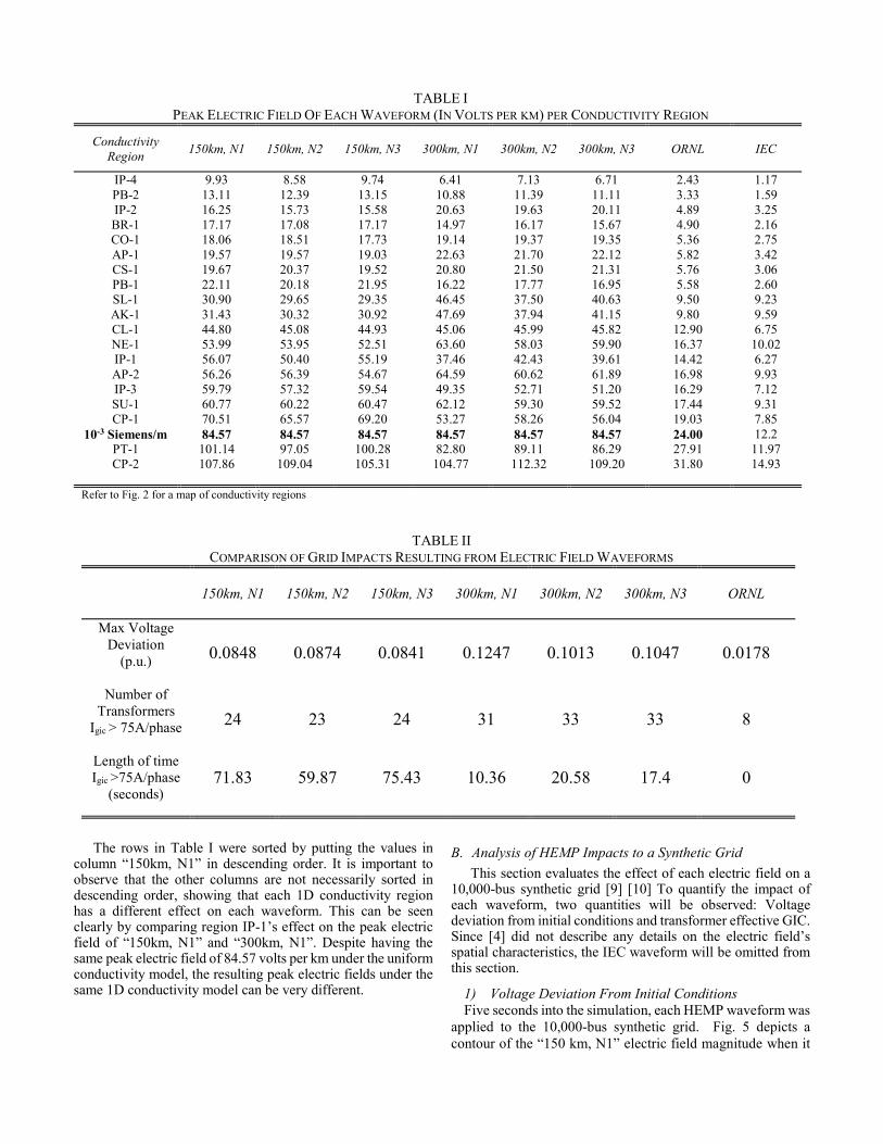
The rows in Table I were sorted by putting the values in column “150km, N1” in descending order. It is important to observe that the other columns are not necessarily sorted in descending order, showing that each 1D conductivity region has a different effect on each waveform. This can be seen clearly by comparing region IP-1’s effect on the peak electric field of “150km, N1” and “300km, N1”. Despite having the same peak electric field of 84.57 volts per km under the uniform conductivity model, the resulting peak electric fields under the same 1D conductivity model can be very different.

B. Analysis of HEMP Impacts to a Synthetic Grid

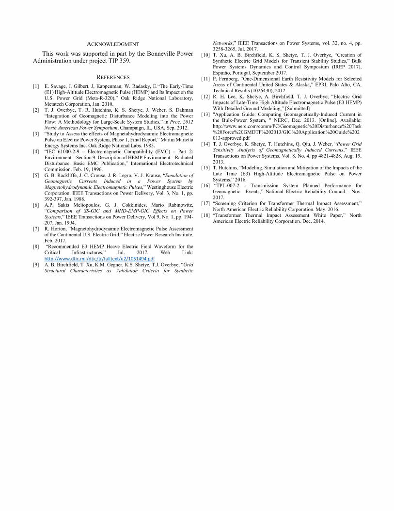
This section evaluates the effect of each electric field on a 10,000-bus synthetic grid [9] [10] To quantify the impact of each waveform, two quantities will be observed: Voltage deviation from initial conditions and transformer effective GIC. Since [4] did not describe any details on the electric field’s spatial characteristics, the IEC waveform will be omitted from this section.

1) Voltage Deviation From Initial Conditions Five seconds into the simulation, each HEMP waveform was

applied to the 10,000-bus synthetic grid. Fig. 5 depicts a contour of the “150 km, N1” electric field magnitude when it

TABLE I PEAK ELECTRIC FIELD OF EACH WAVEFORM (IN VOLTS PER KM) PER CONDUCTIVITY REGION

Conductivity Region

150km, N1

150km, N2

150km, N3 300km, N1

300km, N2

300km, N3

ORNL

IEC

IP-4 9.93 8.58 9.74 6.41 7.13 6.71 2.43 1.17 PB-2 13.11 12.39 13.15 10.88 11.39 11.11 3.33 1.59 IP-2 16.25 15.73 15.58 20.63 19.63 20.11 4.89 3.25 BR-1 17.17 17.08 17.17 14.97 16.17 15.67 4.90 2.16 CO-1 18.06 18.51 17.73 19.14 19.37 19.35 5.36 2.75 AP-1 19.57 19.57 19.03 22.63 21.70 22.12 5.82 3.42 CS-1 19.67 20.37 19.52 20.80 21.50 21.31 5.76 3.06 PB-1 22.11 20.18 21.95 16.22 17.77 16.95 5.58 2.60 SL-1 30.90 29.65 29.35 46.45 37.50 40.63 9.50 9.23 AK-1 31.43 30.32 30.92 47.69 37.94 41.15 9.80 9.59 CL-1 44.80 45.08 44.93 45.06 45.99 45.82 12.90 6.75 NE-1 53.99 53.95 52.51 63.60 58.03 59.90 16.37 10.02 IP-1 56.07 50.40 55.19 37.46 42.43 39.61 14.42 6.27 AP-2 56.26 56.39 54.67 64.59 60.62 61.89 16.98 9.93 IP-3 59.79 57.32 59.54 49.35 52.71 51.20 16.29 7.12 SU-1 60.77 60.22 60.47 62.12 59.30 59.52 17.44 9.31 CP-1 70.51 65.57 69.20 53.27 58.26 56.04 19.03 7.85

10-3 Siemens/m 84.57 84.57 84.57 84.57 84.57 84.57 24.00 12.2 PT-1 101.14 97.05 100.28 82.80 89.11 86.29 27.91 11.97 CP-2 107.86 109.04 105.31 104.77 112.32 109.20 31.80 14.93

Refer to Fig. 2 for a map of conductivity regions

TABLE II COMPARISON OF GRID IMPACTS RESULTING FROM ELECTRIC FIELD WAVEFORMS

150km, N1

150km, N2

150km, N3 300km, N1

300km, N2

300km, N3

ORNL

Max Voltage Deviation

(p.u.)

0.0848 0.0874 0.0841 0.1247 0.1013 0.1047 0.0178

Number of Transformers

Igic > 75A/phase

24 23 24 31 33 33 8

Length of time Igic >75A/phase

(seconds) 71.83 59.87 75.43 10.36 20.58 17.4 0

is at its maximum intensity in relation to the circuit elements of the 10,000-bus synthetic case.

Fig. 6 is a plot of the voltage deviation from initial conditions of a 345kV bus. The “300km, N1” electric field produced the largest amount of voltage deviation while the “150km, N3” electric field produced the lowest. This result confirms previous work which concluded that fast electric field rise times yield higher levels of voltage deviation [15].

The ORNL waveform yielded a maximum voltage drop of only 0.0178 p.u. As expected, it had a much less severe impact on voltage stability compared to the six new waveforms.

Fig. 5. Contour of “150 km, N1” electric field’s magnitude at maximum intensity. The arrows describe the electric field direction. The elements of the 10,000-bus synthetic grid are also shown.

Fig. 6. Plot of a 345kV bus’ voltage deviation from initial conditions during the HEMP simulations

2) Transformer Effective GIC According to [16], transformers which exceed 75 amps per

phase of effective GIC are considered at risk for damage due to transformer hot-spot heating. Reference [17] provides a justification for using 75 amps per phase as a conservative screening criterion. The number of transformers exceeding 75 amps per phase of effective GIC for each waveform is shown on Table II.

The amount of damage sustained by a transformer also depends on the length of time it is exposed to high heat. Furthermore, transformers take time to heat up when exposed to a certain level of effective GIC [18]. Therefore, it is also important to analyze the length of time a transformer is exposed to high levels of effective GIC. The last row of Table II contains the length of time a certain transformer spent above 75 amps per phase of effective GIC. The ORNL waveform caused the observed transformer to reach a peak effective GIC level of only 45.05 amps per phase.

Interestingly, the three 150 km electric field waveforms have low impact considering only the first two rows on Table II. However, they have a greater impact than the other three waveforms regarding the third row’s metric. This is because, despite having slow rise times, the 150km waveforms have sustained levels of high electric field magnitude.

V. CONCLUSION

This paper analyzed HEMP electric field waveforms by converting them to the 1D model to compare their magnitudes at different geographic regions and by applying the fields to a synthetic grid.

In every measure of severity considered in this report, the six waveforms released recently were more severe than the ORNL electric field. This was primarily due to the sheer difference in magnitude between these waveforms.

In some cases, converting different waveforms to the same 1D conductivity region produced in significant differences in the resulting electric field magnitudes. If one HEMP waveform results in a low electric field in a certain region, it does not mean that a different HEMP waveform will also produce low magnitudes in the same region.

When applying the waveforms to a 10,000-bus synthetic grid, the three 300km waveforms yielded the highest levels of voltage deviation and transformer effective GIC. On the other hand, the three 150km waveforms caused the longest sustained high effective GIC levels.

Based on the observations mentioned above, completing a thorough HEMP vulnerability assessment using the new waveforms cannot be done using only one waveform. To protect a grid, whose footprint resides on multiple conductivity regions, against voltage instability and transformer damage, it is important to study the effect of multiple HEMP waveforms to ensure a comprehensive understanding of a grid’s vulnerabilities.

ACKNOWLEDGMENT

This work was supported in part by the Bonneville Power Administration under project TIP 359.

REFERENCES [1] E. Savage, J. Gilbert, J, Kappenman, W. Radasky, E.“The Early-Time

(E1) High-Altitude Electromagnetic Pulse (HEMP) and Its Impact on the U.S. Power Grid (Meta-R-320),” Oak Ridge National Laboratory, Metatech Corporation, Jan. 2010.

[2] T. J. Overbye, T. R. Hutchins, K. S. Shetye, J. Weber, S. Dahman “Integration of Geomagnetic Disturbance Modeling into the Power Flow: A Methodology for Large-Scale System Studies,” in Proc. 2012 North American Power Symposium, Champaign, IL, USA, Sep. 2012.

[3] “Study to Assess the effects of Magnetohydrodynamic Electromagnetic Pulse on Electric Power System, Phase 1, Final Report,” Martin Marietta Energy Systems Inc. Oak Ridge National Labs. 1985.

[4] “IEC 61000-2-9 – Electromagnetic Compatibility (EMC) – Part 2: Environment – Section 9: Description of HEMP Environment – Radiated Disturbance. Basic EMC Publication,” International Electrotechnical Commission. Feb. 19, 1996.

[5] G. B. Rackliffe, J. C. Crouse, J. R. Legro, V. J. Krause, “Simulation of Geomagnetic Currents Induced in a Power System by Magnetohydrodynamic Electromagnetic Pulses,” Westinghouse Electric Corporation. IEEE Transactions on Power Delivery, Vol. 3, No. 1, pp. 392-397, Jan. 1988.

[6] A.P. Sakis Meliopoulos, G. J. Cokkinides, Mario Rabinowitz, “Comparison of SS-GIC and MHD-EMP-GIC Effects on Power Systems,” IEEE Transactions on Power Delivery, Vol 9, No. 1, pp. 194-207, Jan. 1994.

[7] R. Horton, “Magnetohydrodynamic Electromagnetic Pulse Assessment of the Continental U.S. Electric Grid,” Electric Power Research Institute. Feb. 2017.

[8] “Recommended E3 HEMP Heave Electric Field Waveform for the Critical Infrastructures,” Jul. 2017. Web Link: http://www.dtic.mil/dtic/tr/fulltext/u2/1051494.pdf

[9] A. B. Birchfield, T. Xu, K.M. Gegner, K.S. Shetye, T.J. Overbye, “Grid Structural Characteristics as Validation Criteria for Synthetic

Networks,” IEEE Transactions on Power Systems, vol. 32, no. 4, pp. 3258-3265, Jul. 2017.

[10] T. Xu, A. B. Birchfield, K. S. Shetye, T. J. Overbye, “Creation of Synthetic Electric Grid Models for Transient Stability Studies,” Bulk Power Systems Dynamics and Control Symposium (IREP 2017), Espinho, Portugal, September 2017.

[11] P. Fernberg, “One-Dimensional Earth Resistivity Models for Selected Areas of Continental United States & Alaska,” EPRI, Palo Alto, CA, Technical Results (1026430), 2012.

[12] R. H. Lee, K. Shetye, A. Birchfield, T. J. Overbye, “Electric Grid Impacts of Late-Time High Altitude Electromagnetic Pulse (E3 HEMP) With Detailed Ground Modeling,” [Submitted]

[13] "Application Guide: Computing Geomagnetically-Induced Current in the Bulk-Power System, " NERC, Dec. 2013. [Online]. Available: http://www.nerc.com/comm/PC/Geomagnetic%20Disturbance%20Task %20Force%20GMDTF%202013/GIC%20Application%20Guide%202 013-approved.pdf

[14] T. J. Overbye, K. Shetye, T. Hutchins, Q. Qiu, J. Weber, “Power Grid Sensitivity Analysis of Geomagnetically Induced Currents,” IEEE Transactions on Power Systems, Vol. 8, No. 4, pp 4821-4828, Aug. 19, 2013.

[15] T. Hutchins, “Modeling, Simulation and Mitigation of the Impacts of the Late Time (E3) High-Altitude Electromagnetic Pulse on Power Systems.” 2016.

[16] “TPL-007-2 - Transmission System Planned Performance for Geomagnetic Events,” National Electric Reliability Council. Nov. 2017.

[17] “Screening Criterion for Transformer Thermal Impact Assessment,” North American Electric Reliability Corporation. May. 2016.

[18] “Transformer Thermal Impact Assessment White Paper,” North American Electric Reliability Corporation. Dec. 2014.