comparing star formation on large …authors.library.caltech.edu/13713/1/enoapj07.pdfcomparing star...

COMPARING STAR FORMATION ON LARGE SCALES IN THE c2d LEGACY CLOUDS: BOLOCAM1.1 mm DUST CONTINUUM SURVEYS OF SERPENS, PERSEUS, AND OPHIUCHUS

Melissa L. Enoch,1Jason Glenn,

2Neal J. Evans II,

3Anneila I. Sargent,

1

Kaisa E. Young,3,4

and Tracy L. Huard5

Received 2006 November 4; accepted 2007 May 22

ABSTRACT

We have undertaken an unprecedentedly large 1.1 mm continuum survey of three nearby star-forming clouds usingBolocam at the Caltech Submillimeter Observatory. We mapped the largest areas in each cloud at millimeter orsubmillimeter wavelengths to date: 7.5 deg2 in Perseus (Enoch and coworkers), 10.8 deg2 in Ophiuchus (Young andcoworkers), and 1.5 deg2 in Serpens with a resolution of 3100, detecting 122, 44, and 35 cores, respectively. Here wereport on results of the Serpens survey and compare the three clouds. Average measured angular core sizes and theirdependence on resolution suggest that many of the observed sources are consistent with power-law density profiles.Tests of the effects of cloud distance reveal that linear resolution strongly affects measured source sizes and densities,but not the shape of the mass distribution. Core mass distribution slopes in Perseus and Ophiuchus (� ¼ 2:1� 0:1and 2:1� 0:3) are consistent with recent measurements of the stellar IMF, whereas the Serpens distribution is flatter(� ¼ 1:6� 0:2). We also compare the relative mass distribution shapes to predictions from turbulent fragmen-tation simulations. Dense cores constitute less than 10% of the total cloud mass in all three clouds, consistent withother measurements of low star formation efficiencies. Furthermore, most cores are found at high column densities;more than 75% of 1.1 mm cores are associated with AV k 8 mag in Perseus, 15 mag in Serpens, and 20Y23 mag inOphiuchus.

Subject headinggs: ISM: clouds — ISM: individual (Serpens, Perseus, Ophiuchus) — stars: formation —submillimeter

1. INTRODUCTION

Large-scale physical conditions in molecular clouds influencethe outcome of local star formation, including the stellar initialmass function (IMF), star formation efficiency, and the spatial dis-tribution of stars within clouds (e.g., Evans 1999). The physicalprocesses that provide support ofmolecular clouds and control thefragmentation of cloud material into star-forming cores remain amatter of debate. In the classical picture magnetic fields providesupport and collapse occurs via ambipolar diffusion (e.g., Shuet al. 1987), but many simulations now suggest that turbulencedominates both support and fragmentation (for a review seeMacLow & Klessen 2004).

Dense prestellar and protostellar condensations, or cores (fordefinitions and an overview see di Francesco et al. 2007), pro-vide a crucial link between the global processes that control starformation on large scales and the properties of newly formed stars.The mass and spatial distributions of such cores retain imprintsof the fragmentation process, prior to significant influence fromlater protostellar stages such as mass ejection in outflows, coredissipation, and dynamical interactions. These cold (10 K), dense(n > 104 cm�3) cores are most easily observed at millimeter andsubmillimeter wavelengths where continuum emission from colddust becomes optically thin and traces the total mass. Thus, com-plete maps of molecular clouds at millimeter wavelengths are

important for addressing some of the outstanding questions instar formation.Recent advances in millimeter and submillimeter wavelength

continuum detectors have enabled a number of large-scale sur-veys of nearby molecular clouds (e.g., Johnstone et al. 2004;Kirk et al. 2005; Hatchell et al. 2005; Enoch et al. 2006, hereafterPaper I; Stanke et al. 2006; Young et al. 2006, hereafter Paper II ).In addition to tracing the current and future star-forming activityof the clouds on large scales, millimeter and submillimeter obser-vations are essential to understanding the properties of starlesscores and the envelopes of the most deeply embedded protostars(for more on the utility of millimeter observations, see Paper I).We have recently completed 1.1 mm surveys of Perseus

(Paper I ) and Ophiuchus (Paper II ) with Bolocam at the CaltechSubmillimeter Observatory (CSO). In this work we present asimilar 1.1 mm survey of Serpens, completing our three-cloudstudy of nearby northern star-forming molecular clouds. Unlikeprevious work, our surveys not only cover the largest area ineach cloud to date, but the uniform instrumental properties allowa comprehensive comparison of the cloud environments in thesethree regions. A comparison of the results for all three clouds pro-vides insights into global cloud conditions and highlights the in-fluence that cloud environment has on properties of star-formingcores.Background facts on the Perseus and Ophiuchus molecular

clouds are discussed in Papers I and II. The Serpens molecularcloud is an active star formation region at a distance of d¼ 260�10 pc (Straizys et al. 1996). Although the cloud extends morethen 10 deg2 as mapped by optical extinction (Cambresy 1999),most observations of the region have been focused near the mainSerpens cluster at a right ascension (R.A.) of 18h30m and decli-nation (decl.) of 1�150 (J2000.0).The Serpens cluster is a highly extincted region with a high

density of young stellar objects (YSOs), including a number of

1 Division of Physics, Mathematics and Astronomy, California Institute ofTechnology, Pasadena, CA 91125; [email protected].

2 Center for Astrophysics and Space Astronomy, 389-UCB, University ofColorado, Boulder, CO 80309.

3 Astronomy Department, University of Texas, Austin, TX, 78712-0259.4 Department of Physical Sciences, Nicholls State University, Thibodaux,

LA 70301.5 Harvard-Smithsonian Center for Astrophysics, Cambridge, MA 02138.

982

The Astrophysical Journal, 666:982Y1001, 2007 September 10

# 2007. The American Astronomical Society. All rights reserved. Printed in U.S.A.

Class 0 protostars. It has been studied extensively at near-infrared,far-infrared, submillimeter, and millimeter wavelengths (e.g., Eiroa&Casali 1992; Hurt & Barsony 1996; Larsson et al. 2000; Daviset al. 1999; Casali et al. 1993; Testi & Sargent 1998). Some re-cent work has also drawn attention to a less well known clusterto the south, sometimes referred to as Serpens/G3YG6 (Djupviket al. 2006; Harvey et al. 2006). Beyond these two clusters nocontinuum millimeter or submillimeter continuum surveys havebeen done that could shed light on large-scale star formationprocesses.

Following Papers I and II, we utilize the wide-field mappingcapabilities of Bolocam, a large format bolometer array at theCSO, to complete millimeter continuum observations of 1.5 deg2

of the Serpens cloud. These observations are coordinated to coverthe area mapped with Spitzer Space Telescope IRAC and MIPSobservations of Serpens from the ‘‘Cores to Disks’’ (c2d Evanset al. 2003) Legacy project. While millimeter and submillime-ter observations are essential to understanding the properties ofdense prestellar cores and protostellar envelopes, infrared obser-vations are necessary to characterize the protostars embeddedwithin those envelopes. In a future paper (M. Enoch et al. 2007,in preparation) we will take advantage of the overlap betweenour 1.1 mmmaps and the c2d Spitzer Legacy maps to character-ize the deeply embedded and prestellar populations in Serpens.

Here the Bolocam observations and data reduction (x 2), gen-eral cloud morphology and source properties (x 3), and summary(x 4) for Serpens are briefly presented. In x 5 we compare themillimeter survey results for Serpens, Perseus, and Ophiuchus.First, we outline our operational definition of a millimeter coreincluding instrumental effects in x 5.1, and we discuss the obser-vational biases introduced by different cloud distances in x 5.2.Physical implications of source sizes and shapes, as well as dif-ferences between the clouds, are discussed in x 5.3. We examinesource densities and compare the cloud mass versus size distri-butions in x 5.4. We analyze the core mass distributions and theirrelation to cloud turbulence in x 5.5 and the spatial distributionsof the core samples and clustering in x 5.6. The relationship ofdense cores to the surrounding cloud column density and themass fraction in dense cores are discussed in xx 5.7 and 5.8. Weend with a summary in x 6.

2. SERPENS OBSERVATIONS AND DATA REDUCTION

Observations and data reduction for Serpens follow the samemethodology as for Perseus (Paper I) and Ophiuchus (Paper II ).The data reduction techniques we have developed for the molec-ular cloud data are described in detail in Papers I and II, includingremoval of sky noise, construction of pointing and calibrationmodels, application of iterative mapping, and source extraction.Given these previous descriptions, only details specific to Serpenswill be presented here. Further information about the Bolocaminstrument and reduction pipeline is also available in Laurent et al.(2005).

2.1. Observations

As for Perseus and Ophiuchus, millimeter continuum obser-vations of Serpens were made with Bolocam6 at the CSO onMauna Kea, Hawaii. Bolocam is a 144 element bolometer arraythat operates at millimeter wavelengths and is designed to maplarge fields (Glenn et al. 2003). Observations of Serpens werecarried out at a wavelength of k ¼ 1:1 mm, where the field ofview is 7.50 and the beam is well approximated by a Gaussian

with FWHM size of 3100. The instrument has a bandwidth of45 GHz at k ¼ 1:1 mm, excluding the CO (J ¼ 2Y1) line to ap-proximately 99%.

The 1.1mmobservations were designed to cover a regionwithAV � 6 mag in the visual extinction map of Cambresy (1999)shown in Figure 1. As demonstrated in Figure 1, this ensures thatthe Bolocam observations overlap as closely as possible with theregion of Serpens observed with Spitzer IRAC and MIPS as partof the c2d Legacy project. In practice, the Bolocam surveycovers a region slightly larger than the IRAC map and slightlysmaller than the MIPS map.

Serpens was observed during two separate runs in 2003 May21YJune 9 and 2005 June 26Y30. During the 2003 run, 94 of the144 channels were operational, compared to 109 during the 2005run. Scans of Serpens were made at a rate of 6000 s�1 with nochopping of the secondary. The final map consists of 13 scansfrom 2003 in good weather and 17 scans from 2005 in somewhatpoorer conditions. Each scan covered the entire 1.5 deg2 area andtook 35Y40 minutes to complete depending on the scan direc-tion. Scans were made in two orthogonal directions, approxi-mately half in R.A. and half in decl. This strategy allows for goodcross linking in the final map, sub-Nyquist sampling, and mini-mal striping from 1/f noise. Scans were observed in sets of threeoffset by �4300, 000, and +4300 to optimize coverage.

In addition, small maps of pointing sources were observed ap-proximately every 2 hr, and at least one primary flux calibra-tion source, including Neptune, Uranus, andMars, was observed6 See http://www.cso.caltech.edu /bolocam.

Fig. 1.—Bolocam 1.1 mm (thick line) and Spitzer c2d IRAC (thin line) andMIPS (gray line) coverage of Serpens overlaid on the Cambresy (1999) visualextinction map. The area observed with IRACwas chosen to cover AV � 6 magin this portion of the cloud. Our Bolocam survey covers the same area as theIRAC and a slightly smaller area than the MIPS observations.

SURVEYS OF SERPENS, PERSEUS, AND OPHIUCHUS 983

each night. Several larger beam maps of planets were also madeduring each run, to characterize the Bolocam beam at 1.1 mm.

2.2. Pointing and Flux Calibration

A pointing model for Serpens was generated using two nearbypointing sources, G34.3 and the quasar 1749+096. After applica-tion of the pointing model, a comparison to the literature SCUBA850�mpositions offour bright known sources (Davis et al. 1999)in themain Serpens cluster indicated a constant positional offset of(�R:A:; �decl:) ¼ (500; �1000).We corrected for the positional off-set but estimate an uncertainty in the absolute pointing of 1000, stillsmall compared to the beam size of 3100. The relative pointing er-rors, which cause blurring of sources and an increase in the effectivebeam size, should be much smaller, approximately 500. Relativepointing errors are characterized by the rms pointing uncertainty,derived from the deviations of G34.3 from the pointing model.

The Bolocam flux calibration method makes real-time correc-tions for the atmospheric attenuation and bolometer operatingpoint using the bolometer optical loading, by calculating the cal-ibration factor as a function of the bolometer DC resistance. Cal-ibrator maps of Neptune, Uranus, and G34.3, observed at leastonce per night, were used to construct a calibration curve for eachrun. A systematic uncertainty of approximately 10% is associ-ated with the absolute flux calibration, but relative fluxes shouldbe much more accurate.

2.3. Cleaning and Iterative Mapping

Aggressive sky subtraction techniques are required for Bolocamdata to remove sky noise, which dominates over the astronomicalsignal before cleaning. As in Papers I and II, we remove sky noisefrom the Serpens scans using principal component analysis (PCA)cleaning (Laurent et al. 2005 and references therein), by sub-tracting three PCA components.

As described in Paper I, PCA cleaning removes some sourceflux from the map, as well as sky noise, necessitating the use ofan iterative mapping procedure to recover lost astronomical flux.In this procedure, sky subtraction is refined by iteratively re-moving a source model (derived from the cleaned map) from theraw data, thereby reducing contamination of the sky template bybright sources. Simulations show that at least 98% of source fluxdensity is recovered after five iterations, with the exception ofvery large (k10000 FWHM) faint sources, for which we onlyrecover 90% or less of the true flux density (see Paper I). Weconservatively estimate a 10% residual photometric uncertaintyfrom sky subtraction after iterative mapping, in addition to the10% uncertainty in the absolute flux calibration.

Data from the 2003 and 2005 observing runs were iterativelymapped separately because they required different pointing andflux calibration models. After iterative mapping the two epochswere averaged, weighted by the square root of the observationalcoverage.

2.4. Source Identification

Millimeter cores are identified in an optimally filtered mapusing the source extractionmethod described in Paper I. Becausethe signal from a point source lies in a limited frequency band,we can use an optimal (Wiener) filter in Fourier space to atten-uate 1/f noise at low frequencies, as well as high-frequency noiseabove the signal band. The optimal filter preserves the resolutionof the map and the peak brightness of point sources but reducesthe rms noise per pixel by approximately

ffiffiffi3

p, thereby optimiz-

ing the source signal-to-noise ratio (S/N). Extended sources willhave slightly enhanced peak values in the optimally filtered map.After optimal filtering, the map is trimmed to remove areas of

low coverage. Note that the optimally filtered map is used forsource detection only; all photometry is measured in the un-filtered map, and all maps displayed here are unfiltered.Observational coverage, which depends on the scan strategy,

number of scans, and number of bolometer channels, was veryuniform for Serpens; trimming regions where the coverage wasless than 30% of the peak coverage was equivalent to cutting offthe noisy outer edges of the map. The average coverage of theSerpens map is 1600 hits pixel�1, where a hit means a bolometerpassed over this position, with differences in hits per pixel acrossthe map of 18%. The average coverage corresponds to an inte-gration time of 13 minutes pixel�1, although individual pixelsare not independent because the map is oversampled.For each pixel, the local rms noise is calculated in small

(45 arcmin2) boxes using a noise map from which sources havebeen removed. This noise map is derived as part of the iterativemapping process (see Paper I). A simple peak-finding routineidentifies all pixels in the optimally filtered map more than 5 �above the local rms noise level, and source positions are deter-mined using an IDL centroiding routine. Each new source mustbe separated by at least a beam size from any previously identi-fied source centroid. The centroid is a weighted average positionbased on the surface brightness within a specified aperture and iscomputed as the position at which the derivatives of the partialsums of the input image over ( y, x) with respect to (x, y) equalzero. A given centroid is considered ‘‘well defined’’ as long asthe computed derivatives are decreasing. All sources were ad-ditionally inspected by eye to remove spurious peaks near thenoisier edges of the map.

3. SERPENS RESULTS

The final 1000 pixel�1 Serpens map is shown in Figure 2, withthe well-known northern Serpens cluster, cluster A (Harveyet al. 2006), indicated, as well as the southern cluster, cluster B(Serpens/G3YG6). Covering a total area of 1.5 deg2, or 30.9 pc2

at a distance of 260 pc, the map has a linear resolution of7:3 ; 103 AU.We identify 35 sources above the 5 � detection limit in the

Serpens map. The 5 � limit is based on the local rms noise and istypically 50 mJy beam�1. The noise map for Serpens is shownin Figure 3, with the positions of identified sources overlaid.The mean rms noise is 9.5 mJy beam�1 but is higher near brightsources. Most of the 18% variations in the local rms noise occurin the main cluster region, where calculation of the noise is con-fused by residual artifacts from bright sources. Such artifacts mustcontribute significantly to noise fluctuations; coverage variationsalone would predict rms noise variations of only (18)1

=2 ¼ 4%.This means that faint sources near bright regions have a slightlylower chance of being detected than those in isolation.Source positions are listed in Table 1 and identified by red cir-

cles in Figure 4. Figure 4 also shows magnifications of the moredensely populated source regions, including cluster A and clus-ter B.We do not see any circularly symmetric extended emissionon scales k30 in the map. It should, in principle, be possible torecover symmetric structures up to the array size of 7.50, but oursimulations show that sourcesk40 in size are severely affected bycleaning and therefore difficult to fully recover with iterativemapping. The map does contain larger filamentary structures upto 80 long. In particular, the long filament between cluster A andcluster B is reminiscent of the elongated ridge near B1 in Perseus(Paper I). The Serpens filament does not contain the bright compactsources at either end that are seen in the B1 ridge, however.Previous millimeter-wavelength maps of cluster A, such as

the 1.1 mm UKT14 map of Casali et al. (1993) and the 850 �m

ENOCH ET AL.984 Vol. 666

SCUBA map of Davis et al. (1999), generally agree with ourresults in terms of morphology and source structure. Not all ofthe individual 850 �m sources are detected by our peak-findingroutine, presumably due to the poorer resolution of Bolocam(3000) compared to SCUBA (1400), but most can, in fact, be iden-tified by eye in the Bolocam map. An IRAM 1.3 mm continuummap of cluster B with 1100 resolution (Djupvik et al. 2006) is vi-sually quite similar to our Bolocam map of the region. We detecteach of the four 1.3mm sources identified (MMS 1Y4), althoughthe 1.3 mm triplet MMS 1 is seen as a single extended source inour map.

Most of the brightest cores, in particular those in cluster A, areassociated with known YSOs, including a number of Class 0 ob-jects (Hurt &Barsony 1996; Harvey et al. 2006). All bright 1.1mmsources are aligned with bright 160 �m emission in the SpitzerMIPSmap of Serpens observed by the c2d Legacy project (Harveyet al. 2007). Fainter millimeter sources are usually associated withextended 160 �m filaments but do not necessarily correspond topoint sources in the MIPS map. Conversely, one bright extendedregion of 160 �m emission just south of cluster A contains no1.1 mm sources. This area also exhibits extended emission at 70and 24 �m, which may be indicative of warmer, more diffusematerial than that of the dense cores detected at 1.1 mm.

Despite the low rms noise level achieved in Serpens, very fewsources are seen outside the main clusters; most of the area thatwe mapped appears devoid of 1.1 mm emission, despite being ina region of high extinction. Figure 5 shows a comparison between

Fig. 3.—Map of the local 1 � rms noise per beam in the Serpens map. Posi-tions of the 35 sources are indicated by white plus signs. The average rms noiseis 9.5 mJy beam�1, varying by 18% across the map. The noise is higher nearbright sources due to sky subtraction residuals.

Fig. 2.—Bolocam 1.1 mm map of 1.5 deg2 (31 pc 2 at d ¼ 260 pc) in theSerpens molecular cloud. Bolocam has a resolution of 3100, and the map isbinned to 1000 pixel�1. The average 1 � rms noise is 9.5 mJy beam�1.

SURVEYS OF SERPENS, PERSEUS, AND OPHIUCHUS 985No. 2, 2007

the Bolocam millimeter map (gray scale) and visual extinction(contours) derived from c2d near- and mid-infrared Spitzer data.

The majority of sources (90%Y95%) detected by IRAC andMIPS in the c2d clouds have spectral energy distributions (SEDs)characteristic of reddened stars. Thus, we havemeasures of the vi-sual extinction for many lines of sight through themolecular cloudsimaged by c2d. Line-of-sight extinction values are derived byfittingthe RV ¼ 5:5 dust model of Weingartner & Draine (2001) to thenear-infrared through mid-infrared SED (Evans et al. 20067).For each of the three clouds, the derived line-of-sight extinctionswere convolved with uniformly spaced 9000 Gaussian beams toconstruct an extinction map.

Extinction maps used throughout this paper for Serpens, Per-seus, and Ophiuchus are derived from c2d data by this method.The c2d extinction maps accurately trace column densities up toAV � 40 mag but are relatively insensitive to small regions ofhigh volume density because they rely on the detection of back-ground stars. Thus, the extinction maps are complementary to

the 1.1 mm observations, which trace high volume density struc-tures (see x 5.1). In Figure 5, the AV map for Serpens is smoothedto an effective resolution of 2.50.As can be seen in Figure 5, nearly all Serpens millimeter sources

lie within regions of high visual extinction (AV � 10 mag) and, inparticular, all bright Bolocam sources are associated with areasof AV � 15 mag. Nevertheless, there are a number of high ex-tinction areas (AV � 12mag) with no detectable 1.1mm sources.A similar general trend was noted in both Perseus (Paper I) andOphiuchus (Paper II ), with relatively few sources found outsidethe major groups and clusters associated with the highest extinc-tion. In x 5.7 we examine the relationship betweenAV and 1.1mmsources in more detail.

3.1. Source Properties

3.1.1. Positions and Photometry

Positions, peak flux densities, and S/N for the 35 1.1 mmsources identified in the Bolocam map of Serpens are listedin Table 1. The S/N is measured in the optimally filtered map,

TABLE 1

Sources Found in Serpens

ID

R.A.

(J2000.0)

Decl.

(J2000.0)

Peak

(mJy beam�1) S/N Other Names MIPS Source?

Bolo1...................................... 18 28 23.1 +00 26 34.6 95 (12) 5.0 N

Bolo2...................................... 18 28 44.0 +00 53 02.8 198 (12) 9.9 N

Bolo3...................................... 18 28 45.8 +00 51 32.4 227 (12) 13.7 IRAS 18262+0050 Y

Bolo4...................................... 18 28 47.2 +00 50 45.1 145 (10) 7.1 N

Bolo5...................................... 18 28 48.3 +00 14 51.5 73 (9) 5.8 N

Bolo6...................................... 18 28 50.8 +00 50 28.6 115 (10) 7.3 N

Bolo7...................................... 18 28 53.0 +00 19 03.6 119 (11) 5.4 Y

Bolo8...................................... 18 28 55.2 +00 29 28.0 617 (13) 30.8 IRAS 18263+0027; MMS 1 (1) Y

Bolo9...................................... 18 28 55.9 +00 48 30.3 141 (10) 9.1 N

Bolo10.................................... 18 28 56.6 +00 19 10.4 107 (11) 5.7 N

Bolo11.................................... 18 28 57.3 +00 48 06.5 162 (11) 10.9 N

Bolo12.................................... 18 28 58.4 +00 47 35.7 172 (11) 12.0 N

Bolo13.................................... 18 29 00.2 +00 30 19.8 239 (15) 5.5 Y

Bolo14.................................... 18 29 07.0 +00 30 41.5 1016 (14) 59.2 IRAS 18265+0028; MMS 2 (1) Y

Bolo15.................................... 18 29 09.6 +00 31 36.9 626 (14) 33.0 MMS 3 (1) Y

Bolo16.................................... 18 29 13.5 +00 32 12.6 175 (13) 5.8 N

Bolo17.................................... 18 29 16.4 +00 18 15.4 82 (8) 6.7 IRAS 18267+0016 Y

Bolo18.................................... 18 29 19.3 +00 33 29.1 104 (12) 6.0 N

Bolo19.................................... 18 29 31.5 +00 26 49.3 279 (14) 14.8 MMS 4 (1) N

Bolo20.................................... 18 29 31.9 +01 19 00.9 337 (13) 18.3 Y

Bolo21.................................... 18 29 43.4 +00 36 25.2 129 (11) 7.7 N

Bolo22.................................... 18 29 48.8 +01 16 50.6 1694 (16) 80.7 SMM 9 (2); S68N Y

Bolo23.................................... 18 29 50.2 +01 15 24.6 3010 (20) 138 SMM 1 (2); FIRS 1 Y

Bolo24.................................... 18 29 53.8 +00 36 10.1 202 (10) 17.2 IRAS 18273+0034 Y

Bolo25.................................... 18 29 57.4 +01 13 14.9 1980 (23) 62.7 SMM 4 (2) Y

Bolo26.................................... 18 29 59.2 +01 14 07.4 1331 (19) 43.0 SMM 3 (2) Y

Bolo27.................................... 18 30 00.3 +01 10 37.8 425 (19) 14.5 Y

Bolo28.................................... 18 30 00.7 +01 12 56.5 1266 (19) 34.3 SMM 2 (2) Y

Bolo29.................................... 18 30 01.0 +01 11 49.1 979 (19) 33.5 SMM 11 (2) Y

Bolo30.................................... 18 30 02.5 +01 15 24.5 319 (16) 11.3 SMM 8 (2) Y

Bolo31.................................... 18 30 02.8 +01 08 38.3 214 (16) 10.0 Y

Bolo32.................................... 18 30 05.7 +00 39 32.2 105 (12) 5.0 Y

Bolo33.................................... 18 30 06.4 +00 42 37.0 126 (11) 8.3 Y

Bolo34.................................... 18 30 08.2 +01 13 11.5 153 (11) 7.8 N

Bolo35.................................... 18 30 14.7 +01 13 52.6 85 (11) 5.6 N

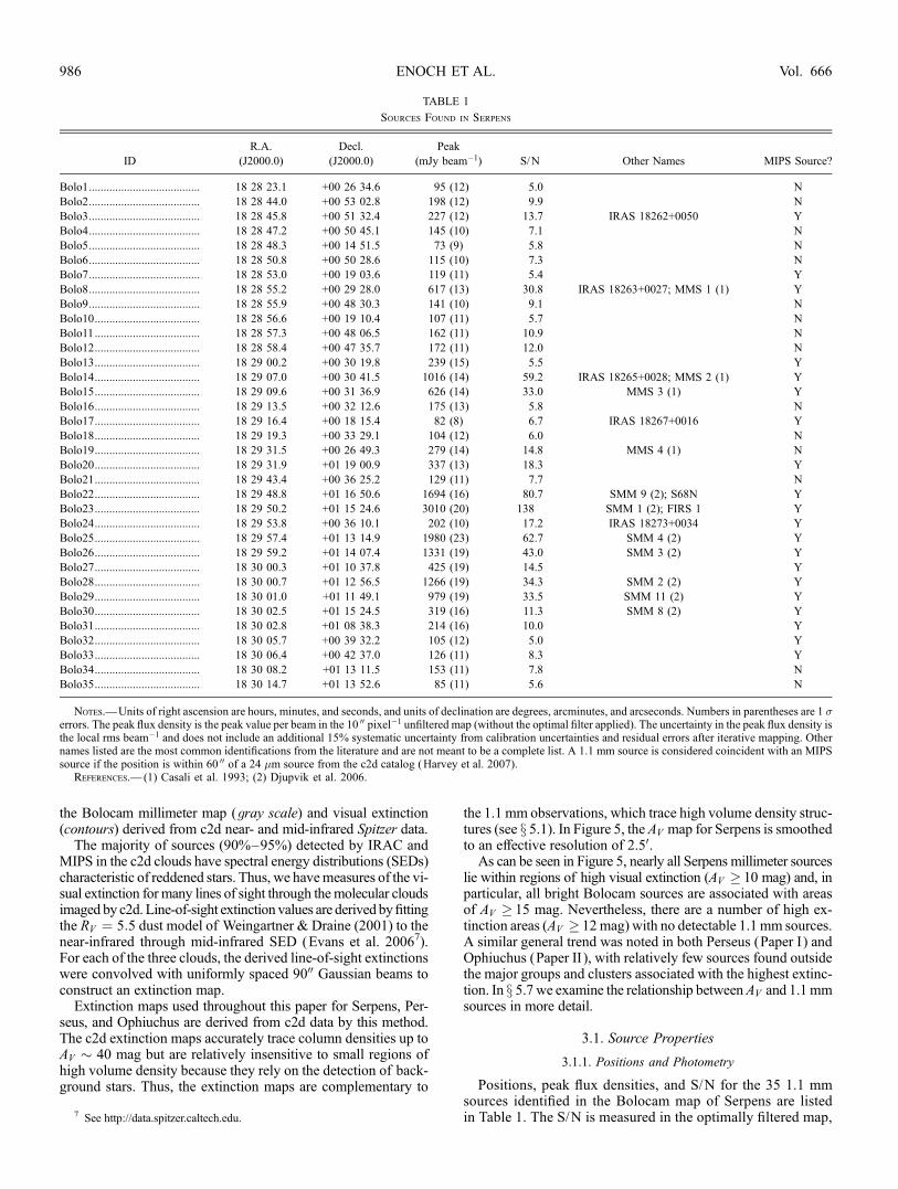
Notes.—Units of right ascension are hours, minutes, and seconds, and units of declination are degrees, arcminutes, and arcseconds. Numbers in parentheses are 1 �errors. The peak flux density is the peak value per beam in the 10 00 pixel�1 unfiltered map (without the optimal filter applied). The uncertainty in the peak flux density isthe local rms beam�1 and does not include an additional 15% systematic uncertainty from calibration uncertainties and residual errors after iterative mapping. Othernames listed are the most common identifications from the literature and are not meant to be a complete list. A 1.1 mm source is considered coincident with an MIPSsource if the position is within 60 00 of a 24 �m source from the c2d catalog (Harvey et al. 2007).

References.— (1) Casali et al. 1993; (2) Djupvik et al. 2006.

7 See http://data.spitzer.caltech.edu.


whereas photometry and all other source properties aremeasuredin the unfiltered, surface brightnessYnormalizedmap. The peak fluxdensity per beam (I�) is given in mJy beam�1 (1 mJy beam�1 ¼0:04 MJy sr�1). Uncertainties in photometry are calculated fromthe local rms beam�1, calculated as in x 2.4. An additional system-atic error of 15% is associated with all flux densities, from theabsolute calibration uncertainty and the systematic bias remainingafter iterativemapping. Table 1 also lists the most commonly usedname from the literature for known sources and indicates if the1.1 mm source is coincident (within 6000) with an MIPS 24 �msource from the c2d database (Harvey et al. 2007).

Table 2 lists photometry in fixed apertures of diameter 4000,8000, and 12000 and the total integrated flux density (S�). Integratedflux densities are measured assuming a sky value of zero and in-clude a correction for the Gaussian beam so that a point source hasthe same integrated flux density in all apertures. No integrated fluxdensity is given if the distance to the nearest neighboring source issmaller than the aperture diameter. The total flux density is inte-grated in the largest aperture (3000Y12000 diameters in steps of 1000)that is smaller than the distance to the nearest neighboring source.

Uncertainties are �ap ¼ �mb(�ap /�mb), where �mb is the localrms beam�1 and (�ap, �mb) are the aperture and beam FWHM,respectively.

Peak and total flux density distributions for the 35 1.1 mmsources in Serpens are shown in Figure 6, with the 5 � detectionlimit indicated. In general, source total flux densities are largerthan peak flux densities because most sources in the map are ex-tended, with sizes larger than the beam. Both distributions lookbimodal; all of the sources in the brighter peak are in either clus-ter A or cluster B. The mean peak flux density of the sample is0.5 Jy beam�1, and themean total flux density is 1.0 Jy, both withlarge standard deviations of order the mean value. Peak AV val-ues of the cores, calculated from the peak flux density as in x 3.1.3,are indicated on the upper axis.

3.1.2. Sizes and Shapes

Source FWHM sizes and position angles (P.A.s, measuredeast of north) are measured by fitting an elliptical Gaussian af-ter masking out nearby sources using a mask radius equal to halfthe distance to the nearest neighbor. The best-fit major- and

Fig. 4.—Bolocam 1.1 mm map of Serpens with the positions of the 35 sources detected above 5 � indicated by red circles. Inset maps magnify the most denselypopulated source regions, including the well-known northern cluster A, cluster B to the south, and an elongated filament reminiscent of the B1 ridge in Perseus (Paper I ).Despite the low rms noise level reached (9.5mJy beam�1), few sources are seen outside the cluster regions.Many bright 1.1mm sources are associatedwithYSOs (Harveyet al. 2006), and all are coincident with 160 �m emission.


minor-axis sizes and P.A.s are listed in Table 2. Errors given arethe formal fitting errors and do not include uncertainties due toresidual cleaning effects, which are of order 10%Y15% for theFWHM and 5

�for the P.A. (see Paper I ).

As can be seen in Figure 7, the minor-axis FWHM values arefairly narrowly distributed around the sample mean of 4900, witha standard deviation of 1200. The major-axis FWHM have a sim-

ilarly narrow distribution with a mean of 6300 and a scatter of 1200.On average sources are slightly elongated, with a mean axis ratioat the half-maximum contour (major-axis FWHM/minor-axisFWHM) of 1.3.Amorphology keyword for each source is also given inTable 2,

to describe the general source shape and environment. Keywordsindicate if the source is multiple (within 30 of another source),extended (major-axis full width at 2 � > 10), elongated (axis ra-tio at 4 � > 1:2), round (axis ratio at 4 � < 1:2), or weak (peakflux densities less than 5 times the rms per pixel in the unfilteredmap). The majority (28/35) of sources are multiple by this def-inition, and nearly all (32/35) are extended at the 2 � contour.

3.1.3. Masses, Densities, and Extinctions

The total massM of gas and dust in a core is proportional to thetotal flux density S� , assuming that the dust emission at 1.1mm isoptically thin and both the dust temperature and opacity areindependent of position within a core:

M ¼ d 2S�

B� TDð Þ��; ð1Þ

where �1:1 mm ¼ 0:0114 cm2 g�1 is the dust opacity per gram ofgas, d ¼ 260 pc is the distance, and TD ¼ 10 K is the dust tem-perature. A gas-to-dust mass ratio of 100 is included in �1:1 mm.The dust opacity is interpolated from Ossenkopf & Henning(1994, Table 1, col. [5]), for dust grains with thin ice mantles,coagulated for 105 yr at a gas density of 106 cm�3. This opacityhas been found to be the best fit in a number of radiative transfermodels (Evans et al. 2001; Shirley et al. 2002; Young et al. 2003,hereafter Y03).Masses calculated in this manner, assuming a dust tempera-

ture of TD ¼ 10 K for all sources, are listed in Table 2. Uncer-tainties given are from the uncertainty in the total flux densityonly; additional uncertainties from �, TD, and d together intro-duce a total uncertainty in the mass of up to a factor of 4 or more(also see Paper I). The dust opacity is uncertain by up to a factorof 2 or more (Ossenkopf & Henning 1994), owing to large uncer-tainties in the assumed dust properties and possible positionalvariations of �� within a core. Variations in both �� and the clouddistance d have smaller effects than dust temperature uncertaintiesfor the range of plausible values (�1:1 mm ¼ 0:005Y0:02 cm2 g�1;d ¼ 200Y300 pc; TD ¼ 5Y30 K).Assuming TD ¼ 10 K is a reasonable compromise to cover

both prestellar and protostellar sources, based on the results ofmore detailed radiative transfermodels (Evans et al. 2001; Shirleyet al. 2002; see also discussion in Paper I). A temperature of 10 Kwill result in overestimates of the masses of protostellar cores,which will be warmer on the inside, by up to a factor of 3 (for a20 K source). Temperature errors are not as problematic as theymight seem, however, as most of the envelope mass is located atlarge radii and low temperatures (see also Paper I).The total mass of the 35 1.1 mm cores in Serpens is 92 M�,

which is only 2.7% of the total cloud mass (3470M�). The cloudmass is estimated from the c2d visual extinction map usingN (H2)/AV ¼ 0:94 ; 1021 mag cm�2 (Bohlin et al. 1978) and

M cloudð Þ ¼ d 2mH�H2�X

N H2ð Þ; ð2Þ

where d is the distance, � is the solid angle,P

indicates sum-mation over all AV > 2 mag pixels in the extinction map, and�H2

¼ 2:8 is the mean molecular weight per H2 molecule.Figure 8 shows the differential mass function of all 1.1 mm

sources in Serpens. The point-source detection limit of 0.13M�

Fig. 5.—Visual extinction (AV ) contours calculated from c2d Spitzer maps,as described in x 3.1.3, overlaid on the gray-scale 1.1 mm map. Contours areAV ¼ 6, 9, 12, 15, 20, and 25 mag and are smoothed to an effective resolution of2.50. All bright 1.1 mm cores are found in regions of high (>15 mag) extinction,but not all high AV areas are associated with strong millimeter sources.

ENOCH ET AL.988

TABLE 2

Photometry and Core Properties

ID

Flux(4000 )

(Jy)

Flux(80 00)

(Jy)

Flux(120 00)

(Jy)

Total Flux

(Jy)

Mass (10 K)

(M�)Peak AV

(mag)

FWHM

(minor)

(arcsec)

FWHM

(major)

(arcsec)

P.A.

(deg)

hni(cm�3) Morphologya

Bolo1........................... 0.137 (0.016) . . . . . . 0.25 (0.03) 0.65 (0.07) 8 52 (1.0) 62 (1.2) 55 (8) 1.0 ; 105 Extended, elongated, weak

Bolo2........................... 0.282 (0.017) . . . . . . 0.51 (0.03) 1.34 (0.08) 17 51 (0.5) 63 (0.6) �57 (4) 2.1 ; 105 Multiple, extended, elongated

Bolo3........................... 0.324 (0.015) . . . . . . 0.382 (0.019) 1.00 (0.05) 19 43 (0.4) 55 (0.5) �77 (3) 3.2 ; 105 Multiple, extended, round

Bolo4........................... 0.226 (0.013) . . . . . . 0.28 (0.017) 0.73 (0.04) 12 43 (0.5) 55 (0.6) 49 (4) 2.2 ; 105 Multiple, extended, elongated

Bolo5........................... 0.094 (0.013) . . . . . . 0.16 (0.02) 0.41 (0.06) 6 50 (1.2) 63 (1.4) �68 (8) 7 ; 104 Extended, round, weak



Bolo8........................... 0.933 (0.018) 1.99 (0.04) . . . 2.63 (0.04) 6.87 (0.12) 52 62 (0.2) 74 (0.2) 68 (1) 5.2 ; 105 Multiple, extended, round

Bolo9........................... . . . . . . . . . 0.169 (0.010) 0.44 (0.03) 12 38 (0.5) 61 (0.7) �58 (2) 1.5 ; 105 Multiple, extended, elongated

Bolo10......................... 0.146 (0.015) . . . . . . 0.146 (0.015) 0.38 (0.04) 9 51 (0.8) 54 (0.9) 11 (25) 8 ; 104 Multiple, extended, elongated

Bolo11......................... . . . . . . . . . 0.199 (0.011) 0.52 (0.03) 14 37 (0.4) 61 (0.7) �59 (2) 1.8 ; 105 Multiple, round

Bolo12......................... 0.246 (0.014) . . . . . . 0.246 (0.014) 0.64 (0.04) 15 39 (0.4) 58 (0.6) �65 (2) 2.2 ; 105 Multiple, extended, elongated

Bolo13......................... 0.36 (0.02) . . . . . . 0.36 (0.02) 0.94 (0.05) 20 52 (0.5) 59 (0.5) �78 (6) 1.7 ; 105 Multiple, extended, round



Bolo16......................... 0.222 (0.018) . . . . . . 0.27 (0.02) 0.71 (0.06) 15 42 (0.5) 62 (0.8) 32 (3) 1.8 ; 105 Multiple, extended, elongated

Bolo17......................... 0.118 (0.011) 0.24 (0.02) 0.4 (0.03) 0.40 (0.03) 1.05 (0.09) 7 80 (1.1) 97 (1.3) �66 (5) 3 ; 104 Extended, elongated

Bolo18......................... 0.144 (0.016) . . . . . . 0.25 (0.03) 0.65 (0.08) 9 48 (0.8) 71 (1.2) �41 (3) 9 ; 104 Multiple, extended, elongated, weak

Bolo19......................... 0.41 (0.018) 0.85 (0.04) 1.28 (0.06) 1.28 (0.06) 3.34 (0.14) 24 74 (0.5) 89 (0.6) �74 (3) 1.3 ; 105 Extended, elongated

Bolo20......................... 0.494 (0.018) 1.01 (0.04) 1.57 (0.05) 1.57 (0.05) 4.11 (0.14) 29 87 (0.5) 90 (0.5) 9 (11) 1.2 ; 105 Extended, elongated

Bolo21......................... 0.177 (0.014) 0.38 (0.03) . . . 0.38 (0.03) 0.98 (0.07) 11 53 (0.7) 64 (0.8) 47 (6) 1.3 ; 105 Multiple, extended, elongated

Bolo22......................... 2.32 (0.02) . . . . . . 3.78 (0.04) 9.86 (0.10) 144 47 (0.1) 57 (0.1) 73 (1) 2.3 ; 106 Multiple, extended, round

Bolo23......................... 3.8 (0.03) 5.91 (0.05) . . . 5.91 (0.05) 15.44 (0.14) 256 46 (0.1) 47 (0.1) 39 (4) 6.1 ; 106 Multiple, extended, round


Bolo25......................... 2.75 (0.03) . . . . . . 3.19 (0.04) 8.33 (0.10) 168 44 (0.1) 51 (0.1) 79 (1) 2.9 ; 106 Multiple, extended, round






Bolo31......................... 0.32 (0.02) 0.65 (0.04) . . . 0.65 (0.04) 1.70 (0.11) 18 45 (0.5) 74 (0.8) �65 (2) 2.4 ; 105 Multiple, extended, elongated

Bolo32......................... 0.151 (0.016) 0.34 (0.03) . . . 0.34 (0.03) 0.88 (0.08) 9 57 (0.9) 74 (1.2) 50 (5) 8 ; 104 Extended, elongated

Bolo33......................... 0.12 (0.015) . . . . . . 0.128 (0.019) 0.34 (0.05) 11 35 (0.9) 39 (1.1) 25 (17) 6.9 ; 106 Round


Bolo35......................... . . . . . . . . . 0.06 (0.011) 0.16 (0.03) 7 24 (1.1) 61 (2.9) �69 (4) 2.4 ; 105 Multiple, weak

Notes.—Masses are calculated according to eq. (1) from the total flux density assuming a single dust temperature of TD ¼ 10 K and a dust opacity at 1.1 mm of �1:1 mm ¼ 0:0114 cm2 g�1. Peak AV is calculated from thepeak flux density as in eq. (3). FWHM and P.A.s are from an elliptical Gaussian fit; the P.A. of the major axis is measured in degrees east of north. Parameter hni is the mean particle density as calculated from the total mass andthe deconvolved average FWHM size. Numbers in parentheses are 1 � uncertainties. Uncertainties for masses are from photometry only and do not include uncertainties from �, TD, or d, which can be up to a factor of a few ormore. Uncertainties for the FWHM and P.A. are formal fitting errors from the elliptical Gaussian fit; additional uncertainties of 10%Y15% apply to the FWHM, and �5� to the P.A. (determined from simulations).

a The morphology keywords given indicate whether the source is multiple (within 30 of another source), extended (major-axis FW at 2 � > 10), elongated (axis ratio at 4 � > 1:2), round (axis ratio at 4 � < 1:2), orweak (peak flux density less than 5 times the rms pixel�1 in the unfiltered map).

is indicated, as well as the 50% completeness limit for sources ofFWHM 5500 (0.35M�), which is the average size of the sample.Completeness is determined from Monte Carlo simulations ofsimulated sources inserted into the raw data and run through thereduction pipeline, as described in Paper I. The best-fit power-law slope to dN /dM / M�� is shown (� ¼ 1:6), as well as thebest-fit lognormal slope.

Our mass distribution has a flatter slope than that found byTesti & Sargent (1998) from higher resolution (500) Owens ValleyRadio Observatory (OVRO) observations (� ¼ �2:1 for M >0:35 M�). This may be due in part to the fact that most of ourdetections, at least 25/35, lie outside the 5:50 ; 5:50 area observedby Testi & Sargent (1998). The resolution differences of the ob-servations may also contribute significantly; for example, a num-ber of our bright sources break down into multiple objects in the500 resolution map.

From the peak flux density I� we calculate the central H2 col-umn density for each source:

N H2ð Þ ¼ I�

�mb�H2mH��B� TDð Þ : ð3Þ

Here �mb is the beam solid angle, mH is the mass of hydrogen,�1:1 mm ¼ 0:0114 cm2 g�1 is the dust opacity per gram of gas, B�

is the Planck function, TD ¼ 10 K is the dust temperature, and�H2

¼ 2:8 as above. From column density we convert to extinc-tion: AV ¼ N (H2)/0:94 ; 1021 mag cm2 (Bohlin et al. 1978),adopting RV ¼ 3:1. We note, however, that this relation was de-termined for the diffuse interstellar medium and may not be idealfor the highly extincted lines of sight probed here.The resulting peakAV values are listed in Table 2. The average

peak AV of the sample is 41 mag with a large standard deviationof 55 mag and a maximum AV of 256 mag. Extinctions calcu-lated from the millimeter emission are generally higher than thosefrom the c2d visual extinctionmap by approximately a factor of 7,likely a combination of both the higher resolution of the Bolocammap (3000 compared with 9000) and the fact that the extinctionmap cannot trace the highest volume densities because it relieson the detection of background sources. Grain growth in densecores beyond that included in the dust opacity fromOssenkopf &Henning (1994) could also lead to an overestimate of the AV fromour 1.1 mm data.Also listed in Table 2 is the mean particle density:

hni ¼ M

4=3ð Þ�R3mH�p

; ð4Þ

whereM is the total mass, R is the linear deconvolved half-widthat half-maximumsize, and�p ¼ 2:33 is themeanmolecularweightper particle. The median of the source mean densities is 2:3 ;105 cm�3, with values ranging from 3:1 ; 104 to 6:1 ; 106 cm�3.

4. SERPENS SUMMARY

We have completed a 1.1 mm dust continuum survey ofSerpens, covering 1.5 deg2, with Bolocam at the CSO.We identify35 1.1 mm sources in Serpens above a 5 � detection limit, whichis 50 mJy beam�1, or 0.13M�, on average. The sample has an av-erage mass of 2.6M� and an average source FWHM size of 5500.

Fig. 6.—Distribution of peak (dashed line) and total (solid line) flux densi-ties of the 35 1.1mm sources in Serpens. PeakAV values derived from the 1.1mmpeak flux densities using eq. (3) are shown on the upper axis. The mean peak fluxdensity of the sample is 0.5 Jy beam�1, themean peak AV is 40mag, and themeantotal flux density is 1.0 Jy. The 5 � detection limit of 0.05 Jy (dotted line) is rela-tively uniform across the cloud.

Fig. 7.—Distribution of source FWHMminor-axis (dashed line) and major-axis (solid line) sizes, determined by an elliptical Gaussian fit. The mean FWHMsizes are 49 00 (minor axis) and 6300 (major axis), and the mean axis ratio (major/minor) is 1.3.

Fig. 8.—Differential mass distribution of the 35 detected 1.1 mm sources inSerpens for masses calculated with TD ¼ 10 K. Dotted lines indicate the point-source detection limit and the empirically derived 50% completeness limit forsources with the average FWHM size of 5500. The best-fit power law (� ¼ 1:6 �0:2) is shown, as well as the best-fit lognormal function.


On average, sources are slightly elongated with a mean axis ratioat half-maximum of 1.3. The differential mass distribution of all35 cores is consistent with a power law of slope � ¼ 1:6� 0:2above 0.35M�. The total mass in dense 1.1 mm cores in Serpens is92 M�, accounting for 2.7% of the total cloud mass, as estimatedfrom our c2d visual extinction map.

5. THREE-CLOUD COMPARISON OF PERSEUS,OPHIUCHUS, AND SERPENS

The survey of Serpens completes a three-cloud study investi-gating the properties of millimeter emission in nearby star-formingmolecular clouds: Perseus (Paper I), Ophiuchus (Paper II ), andSerpens. Having presented the results for the Serpens cloud, wenow compare the three clouds.

Our large-scale millimeter surveys of Perseus, Ophiuchus, andSerpens, completed with the same instrument and reduction tech-niques, provide us with a unique basis for comparing the proper-ties of 1.1mm emission in a variety of star-forming environments.In the following sections we examine similarities and differencesin the samples of star-forming cores and discuss implications forphysical properties of cores and global cloud conditions.

5.1. What is a Core?

Before comparing results from the three clouds, we first de-scribe our operational definition of a millimeter core. The re-sponse of Bolocam to extended emission, together with observedsensitivity limits, determines the type of structure that is detect-able in our 1.1 mmmaps. The Bolocam 1.1 mm observations pre-sented here are sensitive to substructures in molecular cloudswith volume density nk 2 ; 104 cm�3. One way to see this is tocalculate the mean density along the curve defined by the detec-tion as a function of size in each cloud.

Figure 9 demonstrates how the completeness in each cloudvaries as a function of source size. Plotted symbols give the totalmass versus linear deconvolved size for all sources detected ineach cloud, and lines indicate the empirically derived 50% com-pleteness limits. For Ophiuchus the average completeness curveis plotted; as the rms noise varies considerably in Ophiuchus,some regions have higher or lower completeness limits than thecurve shown here. Completeness is determined fromMonte Carlosimulations by adding simulated sources to the raw data, pro-cessing them in the same way as the real data, and attempting todetect them using our peak-finding algorithm (see Paper I). Weare biased against detecting large diffuse sources because wedetect sources based on their peak flux density, whereas the massis calculated from the total flux, which scales approximately asthe size squared.

Calculating mean densities along the 50% completeness curvein each cloud yields nlim � (3Y7) ; 104 cm�3 in Serpens, nlim �(2Y 4) ; 104 cm�3 in Perseus, and nlim � (10Y30) ; 104 cm�3 inOphiuchus. By comparison, the mean cloud density as probedby the extinction map is approximately 1000 cm�3 in Serpens,220 cm�3 in Perseus, and 390 cm�3 in Ophiuchus. To be identi-fied as a core, therefore, individual structures must have a meandensity nk 2 ; 104 cm�3 and a contrast compared to the averagebackground density of at least 30Y100. The mean cloud densityis estimated from the total cloud mass (x 3.1.3) and assumes acloud volume of V ¼ A1:5, where A is the area of the extinctionmap within the AV ¼ 2 contour.

Although we are primarily sensitive to cores with high densitycontrast compared to the background, it is clear that there is struc-ture in the 1.1 mm map at lower contrasts as well, and that manycores are embeddedwithin lower density filaments. The totalmass

in each of the 1.1 mmmaps, calculated from the sum of all pixels>5 �, is approximately twice the mass in dense cores: 176 M�versus 92M� in Serpens, 376M� versus 278M� in Perseus, and83 M� versus 44 M� in Ophiuchus, for ratios of total 1.1 mmmass to total core mass of 1.9, 1.4, and 1.9 respectively. Thus,about half the mass detectable at 1.1 mm is not contained indense cores but is rather in the ‘‘foothills’’ between high-densitycores and the lower density cloud medium.

Structures that meet the above sensitivity criteria and are iden-tified by our peak-finding routine are considered cores. Ourpeak-finding method will cause extended filaments to be brokenup into several separate ‘‘cores’’ if there are local maxima in thefilament separated by more than one beam size, and if each has awell-defined centroid (see x 2.4). There is some question as towhether these objects should be considered separate sources or asingle extended structure, but we believe that our method is morereliable for these data than alternative methods such as Clumpfind(Williams et al. 1994). In Paper I we found that faint extendedsources in our maps, which one would consider single if ex-amining by eye, are often partitioned into multiple sources byClumpfind. Using ourmethod, one filamentary structure in Serpensis broken up into several sources, as are two filaments in Perseus.

Monte Carlo tests were done to quantify biases and systematicerrors introduced by the cleaning and iterative mapping process,which affect the kind of structure we can detect. Measured FWHM,axis ratios, and P.A.s are not significantly affected by eithercleaning or iterative mapping for sources with FWHM P12000;likewise, any loss of flux for such sources has an amplitude lessthan that of the rms noise. Sources with FWHMk 20000 are de-tected, but with reduced flux density (by up to 50%) and largeerrors in the measured FWHM sizes of up to a factor of 2.

The limitation on measurable core sizes of approximately 12000

corresponds to 3 ; 104 AU in Perseus and Serpens and 1:5 ;104 AU in Ophiuchus. Note that these sizes are of order themedian core separation in each cloud (see x 5.6), meaning thatwe are just as likely to be limited by the crowding of cores as byour sensitivity limits in the measurement of large cores. The de-pendence of measurable core size on cloud distance can be seen

Fig. 9.—Completeness as a function of linear deconvolved source size inSerpens, Perseus, andOphiuchus. Symbols show the distribution of sourcemassvs. deconvolved size in each of the three clouds, where the size is the linear de-convolved average FWHM. Lines are empirical 50% completeness limits de-termined from Monte Carlo simulations and demonstrate the dependence ofcompleteness on source size and cloud distance. The beam FWHM of 3100 cor-responds to approximately 8 ; 103 AU in Serpens and Perseus and 4 ; 103 AUin Ophiuchus. Error bars for average-sized sources near the detection limit ineach cloud are also shown, as estimated from the results of Monte Carlo simula-tions and pointing uncertainties of approximately 1000.


in Figure 9, where the completeness rises steeply at smaller lineardeconvolved sizes for Ophiuchus than for Perseus or Serpens.Thus, we are biased against measuring large cores in Ophiuchuscompared to the other two clouds. Although there are cores inour sample with sizes up to 3 ; 104 AU (Fig. 9), most cores havesizes substantially smaller than the largest measurable value,again indicating that we are not limited by systematics.

To summarize, the Bolocam 1.1 mm observations presentedhere naturally pick out substructures in molecular clouds withhigh volume density (nk2 ; 104 cm�3). These millimeter coreshave a contrast of at least 30Y100 compared to the average clouddensity as measured by the visual extinction map [(2Y10) ;103 cm�3]. Many cores are embedded in lower density extendedstructures, which contribute approximately half the mass mea-surable in the Bolocam 1.1 mmmaps. Finally, Monte Carlo testsindicate that we can detect cores with intrinsic sizes up to approx-imately 12000.

5.2. Distance Effects

To test the effects of instrumental resolution and its depen-dence on distance, we convolve the Ophiuchus map with a largerbeam to simulate putting it at approximately the same distance as

Perseus and Serpens. After convolving the unfiltered Ophiuchusmap to 6200 resolution, we apply the optimal filter and recomputethe local rms noise, as described for Serpens (x 2.4). The pixelscale in the convolved map is still 1000 pixel�1, but the resolutionis now 6200 and the rms is lower than in the original map, witha median value of 17 mJy beam�1 in the main L1688 region.Source detection and photometry are carried out in the same wayas for the original map, with the exception that a 6200 beam isassumed.We detect 26 sources in the degraded-resolution map, or 40%

fewer than the 44 sources in the original map. Therefore, a num-ber of sources do become confused at lower resolution. The basicsource properties for the original and degraded-resolution sam-ples, including angular deconvolved sizes, axis ratios, mass dis-tribution, and mean densities, are compared in Figure 10. Herethe angular deconvolved size is defined as �dec ¼ (�2

meas � B2)1=2,

where �meas is the geometric mean of the measured minor- andmajor-axis FWHM sizes and B is the pointing-smeared beamFWHM (32.500 and 6200 for the original and degraded-resolutionmaps, respectively).We note that the average source size in the degraded-resolution

map is nearly twice that in the original Ophiuchus map (average

Fig. 10.—Comparison of the basic source properties for the original (black histogram) and degraded-resolution, or convolved (gray hatched histogram), Ophiuchussource samples, which contain 44 and 26 cores, respectively. (a) Measured angular deconvolved sizes are larger in the degraded-resolution map than in the original mapby approximately a factor of 2 (respective mean values of 9800 and 6100). (b) Sources tend to be slightly more elongated in the degraded-resolution map, with an averageaxis ratio of 1:3� 0:2 compared to 1:2� 0:2 in the original map. (c) The slope of the CMD is not significantly changed for the degraded-resolution sample, but a numberof low-mass cores are blended into a few higher mass sources. (d ) Larger deconvolved sizes lead to lower mean densities for the degraded-resolution sample (medianvalues of 1:6 ; 105 and 5:8 ; 105 cm�3).


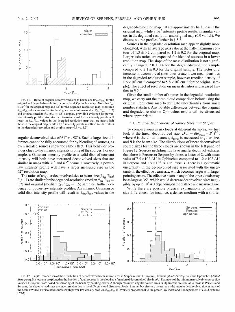
angular deconvolved size of 6100 vs. 9800). Such a large size dif-ference cannot be fully accounted for by blending of sources, aseven isolated sources show the same effect. This behavior pro-vides clues to the intrinsic intensity profile of the sources. For ex-ample, a Gaussian intensity profile or a solid disk of constantintensity will both have measured deconvolved sizes that aresimilar in maps with 3100 and 6200 beams. Conversely, a power-law intensity profile will have a larger measured size in the6200 resolution map.

The ratios of angular deconvolved size to beam size (�dec /�mb;Fig. 11) are similar for the degraded-resolution (median �dec /�mb ¼1:7) and original (median �dec /�mb ¼ 1:5) samples, further evi-dence for power-law intensity profiles. An intrinsic Gaussian orsolid disk intensity profile will result in �dec /�mb values in the

degraded-resolution map that are approximately half those in theoriginal map, while a 1/r2 intensity profile results in similar val-ues in the degraded-resolution and original map (0.9 vs. 1.3). Wediscuss source profiles further in x 5.3.

Sources in the degraded-resolution map appear slightly moreelongated, with an average axis ratio at the half-maximum con-tour of 1:3� 0:2 compared to 1:2� 0:2 for the original map.Larger axis ratios are expected for blended sources in a lowerresolution map. The slope of the mass distribution is not signifi-cantly changed: 2:0� 0:4 for the degraded-resolution samplecompared to 2:1� 0:3 for the original sample. The factor of 2increase in deconvolved sizes does create lower mean densitiesin the degraded-resolution sample, however (median density of1:6 ; 105 cm�3 compared to 5:8 ; 105 cm�3 for the original sam-ple). The effect of resolution on mean densities is discussed fur-ther in x 5.4.

Given the small number of sources in the degraded-resolutionmap, we carry out the three-cloud comparison below using theoriginal Ophiuchus map to mitigate uncertainties from smallnumber statistics. Any notable differences between the originaland degraded-resolution Ophiuchus results will be discussedwhere appropriate.

5.3. Physical Implications of Source Sizes and Shapes

To compare sources in clouds at different distances, we firstlook at the linear deconvolved size: Ddec ¼ d(�2

meas � B2)1=2,

where d is the cloud distance, �meas is measured angular size,and B is the beam size. The distributions of linear deconvolvedsource sizes for the three clouds are shown in the left panel ofFigure 12. Sources inOphiuchus have smaller deconvolved sizesthan those in Perseus or Serpens by almost a factor of 2, with meanvales of 7:5 ; 103 AU in Ophiuchus compared to 1:2 ; 104 AUin Serpens and 1:5 ; 104 AU in Perseus. There is a systematicuncertainty in the deconvolved size associated with the uncer-tainty in the effective beam size, which becomes larger with largerpointing errors. The effective beam in any of the three clouds maybe as large as 3500, whichwould decrease deconvolved sizes negli-gibly, by up to 103AUdepending on the distance andmeasured size.

While there are possible physical explanations for intrinsicsize differences, for instance, a denser medium with a shorter

Fig. 11.—Ratio of angular deconvolved size to beam size (�dec /�mb) for theoriginal and degraded-resolution, or convolved, Ophiuchus maps. Note that �mb

is 3100 for the original map and 6200 for the degraded-resolution map. Measured�dec /�mb values are similar for the degraded-resolution (median �dec /�mb ¼ 1:7)and original (median �dec /�mb ¼ 1:5) samples, providing evidence for power-law intensity profiles. An intrinsic Gaussian or solid disk intensity profile willresult in �dec /�mb values in the degraded-resolution map that are nearly halfthose in the original map, while a 1/r 2 intensity profile results in similar valuesin the degraded-resolution and original map (0.9 vs. 1.3).

Fig. 12.—Left : Comparison of the distribution of deconvolved linear source sizes in Serpens (solid histogram), Perseus (shaded histogram), and Ophiuchus (dottedhistogram). Histograms are plotted as the fraction of total sources in the cloud as a function of deconvolved size in AU. Estimates of the minimum resolvable source size(dashed histograms) are based on smearing of the beam by pointing errors. Although measured angular source sizes in Ophiuchus are similar to those in Perseus andSerpens, the deconvolved sizes are much smaller due to the different cloud distances. Right : Similar, but sizes are measured as the angular deconvolved size in units ofthe beam FWHM. For isolated sources with power-law density profiles, �dec /�mb is inversely proportional to the power-law index and is independent of cloud distance(Y03).


Jeans length should produce smaller cores on average, we aremore likely seeing a consequence of the higher linear resolutionin Ophiuchus, as discussed in x 5.2. Thus, cores in Serpens andPerseus would likely appear smaller if observed at higher resolu-tion, and measured linear deconvolved sizes should be regardedas upper limits. To reduce the effects of distance, we examine theratio of angular deconvolved size to beam size (�dec /�mb; Fig. 12,right panel ). We found in x 5.2 that �dec /�mb does not dependstrongly on the linear resolution but does depend on the intrinsicsource intensity profile.

If the millimeter sources follow power-law density distribu-tions, which do not have a well-defined size, then Y03 show that�dec /�mb depends on the index of the power law, and not on thedistance of the source. So, for example, if sources in Perseus andOphiuchus have the same intrinsic power-law profile, the mean�dec /�mb should be similar in the two clouds, and the mean lineardeconvolved size should be twice as small in Ophiuchus becauseit lies at half the distance. This is precisely the behavior we ob-serve, suggesting that many of the detected 1.1 mm sources havepower-law density profiles.

Considering that a number of the 1.1 mm sources have internalluminosity sources (M. Enoch et al. 2007, in preparation) andthat protostellar envelopes are oftenwell described by power-lawprofiles (Shirley et al. 2002; Y03), this is certainly a plausiblescenario. According to the correlation between �dec and den-sity power-law exponent p found by Y03, median �dec /�mb valuesof 1.7 in Perseus, 1.5 in Ophiuchus, and 1.3 in Serpens would im-ply average indices of p ¼ 1:4, 1.5, and 1.6 respectively. Thesenumbers are consistent with mean p-values found from radia-tive transfer modeling of Class 0 and Class I envelopes ( p � 1:6;Shirley et al. 2002; Y03), although the median for those samplesis somewhat higher ( p � 1:8). Note that source profiles coulddeviate from a power law on scales much smaller than the beamsize, or on scales larger than our size sensitivity (20000), withoutaffecting our conclusions.

Perseus displays the widest dispersion of angular sizes, rang-ing continuously from 1�mb to 4�mb. By contrast, more than halfthe sources in Serpens and Ophiuchus are within 0.5�mb of theirrespective mean values. Although there is a group of Ophiuchussources at large sizes in Figure 12, note that the degraded-resolutionOphiuchus sample displays a very narrow range of sizes (Fig. 11),similar to Serpens. The observed size range in Perseus wouldcorrespond to a wide range of power-law indices, from very shal-low ( p � 1) to that of a singular isothermal sphere ( p ¼ 2). Amore likely possibility, however, is that sourceswith large �dec/�mb

do not follow power-law density profiles.The axis ratio at the half-maximum contour is a simple mea-

sure of source shape. Figure 13 shows the distribution of 1.1 mmsource axis ratios in the three clouds. Our simulations suggestthat axis ratios of up to 1.2 can be introduced by the data reduc-tion (Paper I), so we consider sources with an axis ratio <1.2 tobe round and those with a ratio >1.2 to be elongated. Sources inOphiuchus tend to be round, with a mean axis ratio of 1.2, butnote that themean axis ratio in the degraded-resolutionOphiuchussample is 1.3. The average axis ratio in Serpens is 1.3, and Perseussources exhibit the largest axis ratios with a mean of 1.4 and a tailout to 2.7.

We found in Paper II that Ophiuchus sources were more elon-gated at the 4 � contour than at the half-maximum contour, aswould be the case for round cores embedded in more elongatedfilaments. A similar situation is seen in Serpens; the average axisratio at the 4 � contour is 1.4 in all three clouds. Thus, cores inPerseus are somewhat elongated on average, while objects inSerpens and Ophiuchus appear more round at the half-maximum

contour but elongated at the 4 � contour, suggesting round coresembedded in filamentary structures.In addition to angular sizes, Y03 also note a relationship be-

tween axis ratio and density power-law exponent, finding thataspherical sources are best modeled with shallower density pro-files. The inverse proportionality between p and axis ratio dem-onstrated in Figure 25 of Y03 suggests power-law indices in allthree clouds between 1.5 and 1.7. These values are consistentwith those inferred from the average angular deconvolved sourcesizes, and the wider variation of axis ratios in Perseus againpoints to a larger range in p for that cloud.

5.4. Densities and the Mass versus Size Distribution

Mean densities calculated using linear deconvolved FWHMsizes appear to be significantly higher in Ophiuchus, where themedian of the mean densities of the sample is 5:4 ; 105 cm�3,than in Serpens (median density 2:2 ; 105 cm�3) or Perseus (me-dian density 1:6 ; 105 cm�3), as seen in the left panel of Fig-ure 14. There is a large scatter with standard deviation of ordertwice the mean value in all three clouds. Sources in Ophiuchustend to be less massive than in the other two clouds, so the largermean densities can be entirely attributed to smaller deconvolvedsizes in the Ophiuchus sample, which are sensitive to the shapeof the intrinsic density distribution (Y03). As noted in x 5.2, lin-ear resolution has a strong systematic effect on deconvolvedsizes, and consequently on mean densities. The median densityof the degraded-resolution Ophiuchus sample is 1:6 ; 105 cm�3,similar to both Perseus and Serpens.We additionally calculate mean densities using the full width

at 4 � size rather than the FWHM size (Fig. 14, right panel ) totest the hypothesis that mean density differences are largely aneffect of how source sizes are measured. Using this definition,differences between the clouds are less pronounced, with mediandensities of 1:2 ; 105 cm�3 in Perseus, 1:3 ; 105 cm�3 in Serpens,and 2:0 ; 105 cm�3 in Ophiuchus. These numbers suggest thatsource mean densities are less dependent on cloud distance whenmeasured at the radius where the source merges into the back-ground, rather than at the half-maximum.Figure 15 again displays the source total mass versus size

distribution, using the angular deconvolved size (�dec , in units ofthe beam size) rather than the linear deconvolved size. With the

Fig. 13.—Comparison of the distribution of axis ratios, where the ratio iscalculated at the half-maximum contour. Axis ratios<1.2 are considered round,and >1.2 elongated, based on Monte Carlo simulations. Sources are primarilyround in Ophiuchus and Serpens, with mean axis ratio of 1.2 and 1.3, respec-tively. Perseus exhibits the most elongated sources, with a mean axis ratio of 1.4and a distribution tail extending up to 2.7.


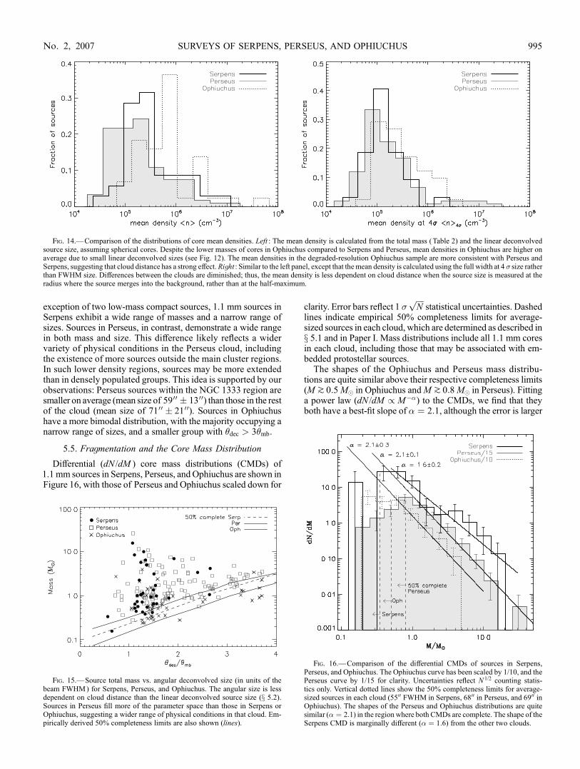
exception of two low-mass compact sources, 1.1 mm sources inSerpens exhibit a wide range of masses and a narrow range ofsizes. Sources in Perseus, in contrast, demonstrate a wide rangein both mass and size. This difference likely reflects a widervariety of physical conditions in the Perseus cloud, includingthe existence of more sources outside the main cluster regions.In such lower density regions, sources may be more extendedthan in densely populated groups. This idea is supported by ourobservations: Perseus sources within the NGC 1333 region aresmaller on average (mean size of 5900 � 1300) than those in the restof the cloud (mean size of 7100 � 2100). Sources in Ophiuchushave a more bimodal distribution, with the majority occupying anarrow range of sizes, and a smaller group with �dec > 3�mb.

5.5. Fragmentation and the Core Mass Distribution

Differential (dN /dM ) core mass distributions (CMDs) of1.1mm sources in Serpens, Perseus, and Ophiuchus are shown inFigure 16, with those of Perseus and Ophiuchus scaled down for

clarity. Error bars reflect 1 �ffiffiffiffiN

pstatistical uncertainties. Dashed

lines indicate empirical 50% completeness limits for average-sized sources in each cloud, which are determined as described inx 5.1 and in Paper I. Mass distributions include all 1.1 mm coresin each cloud, including those that may be associated with em-bedded protostellar sources.

The shapes of the Ophiuchus and Perseus mass distribu-tions are quite similar above their respective completeness limits(M k 0:5M� in Ophiuchus andM k 0:8M� in Perseus). Fittinga power law (dN /dM / M��) to the CMDs, we find that theyboth have a best-fit slope of � ¼ 2:1, although the error is larger

Fig. 15.—Source total mass vs. angular deconvolved size (in units of thebeam FWHM) for Serpens, Perseus, and Ophiuchus. The angular size is lessdependent on cloud distance than the linear deconvolved source size (x 5.2).Sources in Perseus fill more of the parameter space than those in Serpens orOphiuchus, suggesting a wider range of physical conditions in that cloud. Em-pirically derived 50% completeness limits are also shown (lines).

Fig. 16.—Comparison of the differential CMDs of sources in Serpens,Perseus, and Ophiuchus. The Ophiuchus curve has been scaled by 1/10, and thePerseus curve by 1/15 for clarity. Uncertainties reflect N 1/2 counting statis-tics only. Vertical dotted lines show the 50% completeness limits for average-sized sources in each cloud (5500 FWHM in Serpens, 6800 in Perseus, and 6900 inOphiuchus). The shapes of the Perseus and Ophiuchus distributions are quitesimilar (� ¼ 2:1) in the region where both CMDs are complete. The shape of theSerpens CMD is marginally different (� ¼ 1:6) from the other two clouds.

Fig. 14.—Comparison of the distributions of core mean densities. Left : The mean density is calculated from the total mass (Table 2) and the linear deconvolvedsource size, assuming spherical cores. Despite the lower masses of cores in Ophiuchus compared to Serpens and Perseus, mean densities in Ophiuchus are higher onaverage due to small linear deconvolved sizes (see Fig. 12). The mean densities in the degraded-resolution Ophiuchus sample are more consistent with Perseus andSerpens, suggesting that cloud distance has a strong effect. Right : Similar to the left panel, except that the mean density is calculated using the full width at 4 � size ratherthan FWHM size. Differences between the clouds are diminished; thus, the mean density is less dependent on cloud distance when the source size is measured at theradius where the source merges into the background, rather than at the half-maximum.


on the slope for Ophiuchus (�� ¼ 0:3) than for Perseus (�� ¼0:1). The slope of the Serpens CMD is marginally different (� ¼1:6� 0:2), being flatter than in the other two clouds by approx-imately 2 �.

The two-sided Kolmogorov-Smirnov test indicates a highprobability (46%) that the Perseus and Ophiuchus mass distri-butions are representative of the same parent population. Con-versely, the probabilities that the Serpens coremasses are sampledfrom the same population as the Perseus (probability 12%) orOphiuchus (probability 5%) masses are much lower. Although itis possible that the lower linear resolution in Perseus and Serpenshas led to larger masses via blending, the test we conducted to in-crease the effective beam size in the Ophiuchus map did not ap-preciably change the shape of the Ophiuchus mass distribution(see Fig. 10).

If the shape of the CMD is a result of the fragmentation pro-cess, then the slope of the CMD can be compared to models, e.g.,of turbulent fragmentation. Padoan & Nordlund (2002) arguethat turbulent fragmentation naturally produces a power lawwith� ¼ 2:3, consistent with the slopes we measure in Perseus andOphiuchus (� ¼ 2:1), but not with Serpens (� ¼ 1:6). RecentlyBallesteros-Paredes et al. (2006, hereafter BP06) have ques-tioned that result, finding that the shape of the CMD dependsstrongly on the Mach number of the turbulence in their simula-tions. The BP06 smoothed particle hydrodynamics (SPH) simula-tions show that higherMach numbers result in a larger number ofsources with lower mass and a steep slope at the high-mass end(their Fig. 5). Conversely, lower Mach numbers favor sourceswith higher mass, resulting in a smaller number of low-masssources, more high-mass cores, and a shallower slope at the high-mass end.

Using an analytic argument, Padoan & Nordlund (2002) alsonote a relationship between core masses andMach numbers, pre-dicting that the mass of the largest core formed by turbulentfragmentation should be inversely proportional to the square ofthe Alfvenic Mach number on the largest turbulent scale,M2

A.Given that our ability to accurately measure the maximum coremass is limited by resolution, small number statistics, and clouddistance differences, we focus here on the overall CMD shapes.

To compare our observational results to the simulations ofBP06, we estimate the sonic Mach number M ¼ �v /cs in eachcloud. Here �v is the observed rms velocity dispersion, cs ¼(kT /�mH)

1=2 is the isothermal sound speed, and � ¼ 2:33 is themean molecular weight per particle. Large 13CO maps of Perseusand Ophiuchus observed with FCRAO at a resolution of 4400 arepublicly available as part of ‘‘The COMPLETE Survey of StarForming Regions’’8 (COMPLETE; Goodman et al. 2004; Ridgeet al. 2006). Average observed rms velocity dispersions kindlyprovided by the COMPLETE team are �v ¼ 0:68 km s�1 inPerseus, �v ¼ 0:44 km s�1 in Ophiuchus, and �v ¼ 0:92 km s�1

in Serpens (J. Pineda 2006, private communication). These weremeasured by masking out all positions in the map that have peaktemperatures with an S/N less than 10, fitting a Gaussian profileto each, and taking an average of the standard deviations.

We note that the value of �v ¼ 0:68 km s�1 for Perseus issmaller than a previous measurement of �v ¼ 2:0 km s�1 basedon AT&T Bell Laboratory 7 m observations of a similar area ofthe cloud (Padoan et al. 2003). The smaller value derived by theCOMPLETE team is most likely a consequence of the methodused: a line width is calculated at every position and then an av-erage of these values is taken. In contrast to calculating the widthof the averaged spectrum, this method removes the effects of

velocity gradients across the cloud. The different resolutions ofthe surveys (4400 and 0.07 km s�1 for the COMPLETE observa-tions, 10000 and 0.27 km s�1 for the Padoan et al. [2003] obser-vations) may also play a role. Sources of uncertainty in the linewidth measurement are not insignificant and include the possi-bility that 13CO is optically thick to an unknown degree and thefact that line profiles are not necessarily well fitted by aGaussian,especially in Perseus, where the lines sometimes appear doublepeaked.Assuming that the sound speed is similar in all three clouds,

the relative velocity dispersions suggest that turbulence is moreimportant in Serpens than in Perseus or Ophiuchus, by factors ofapproximately 1.5 and 2, respectively. Mach numbers calculatedusing the observed �v and assuming a gas kinetic temperature of10 K areM ¼ 4:9 (Serpens),M ¼ 3:6 (Perseus), andM ¼ 2:3(Ophiuchus). We focus on Serpens and Ophiuchus, as they arethe most different. Serpens is observed to have a higher Machnumber than Ophiuchus, but the CMD indicates a larger numberof high-mass cores, a shallower slope at the high-mass end, and adearth of low-mass cores compared to Ophiuchus. This result iscontrary to the trends found by BP06, which would predict asteeper slope and more low-mass cores in Serpens.9

One core of relatively high mass is measured in the degraded-resolution map of Ophiuchus, as is expected for blending atlower resolution (Fig. 10), making the difference between theSerpens and Ophiuchus CMDs less dramatic. The degraded-resolution CMD for Ophiuchus still has a steeper slope (� ¼2:0� 0:4) than the Serpens CMD, however, and a larger fractionof low-mass sources: 81% of sources in the degraded-resolutionOphiuchus sample have M < 2 M� compared to 49% in theSerpens sample.More accurate measurements of the Mach number and higher

resolution studies of the relative CMD shapes will be necessaryto fully test the BP06 prediction, given that uncertainties are cur-rently too large to draw firm conclusions. As both numerical sim-ulations and observations improve, however, the observed CMDand measurements of the Mach number will provide a powerfulconstraint on turbulent star formation simulations.Comparing the shape of the CMD to the stellar IMF may give

insight into what determines final stellar masses: the initial frag-mentation into cores, competitive accretion, or feedback pro-cesses. The shape of the local IMF is still uncertain (Scalo 2005),but recent work has found evidence for a slope of � ¼ 2:5Y2:8for stellar masses M k 1 M�, somewhat steeper than the slopeswe observe in all three clouds. For example, Reid et al. (2002)find � ¼ 2:5 above 0.6 M� and � ¼ 2:8 above 1 M�. Chabrier(2003) suggests � ¼ 2:7 (M > 1 M�), while Schroder & Pagel(2003) find � ¼ 2:7 for 1:1 M� < M < 1:6 M� and � ¼ 3:1for 1:6 M� < M < 4 M�. For reference, the Salpeter IMF has aslope of � ¼ 2:35 (Salpeter 1955).For comparison to the IMF, we would ideally like to construct

a CMD that includes starless cores only, so that it is a measure ofthe mass initially available to form a star. Although we cannotseparate prestellar cores from more evolved objects with milli-meter data alone, we are currently comparing the Bolocam mapswith c2d Spitzer Legacy maps of the same regions, which willallow us to distinguish prestellar cores from those with internalluminosity sources (M. Enoch et al. 2007, in preparation).

8 See http://cfa-www.harvard.edu/COMPLETE/.

9 It should be noted that the shape of the CMDs presented by BP06 dependson the type of numerical code used, and not on the cloud Mach number alone.Here we have compared to the BP06 SPH simulations (their Fig. 5); for the BP06total variation diminishing (TVD) method (their Fig. 4), a larger number of low-mass cores are again seen for higher Mach numbers, but the CMD slopes at thehigh-mass end are independent of Mach number.


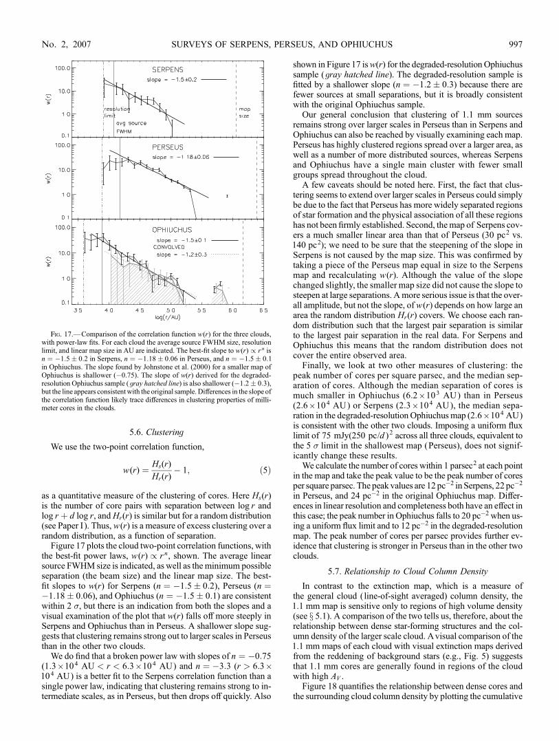
5.6. Clustering

We use the two-point correlation function,

w(r) ¼ Hs(r)

Hr(r)� 1; ð5Þ

as a quantitative measure of the clustering of cores. Here Hs(r)is the number of core pairs with separation between log r andlog r þ d log r, andHr(r) is similar but for a random distribution(see Paper I ). Thus, w(r) is a measure of excess clustering over arandom distribution, as a function of separation.

Figure 17 plots the cloud two-point correlation functions, withthe best-fit power laws, w(r) / r n, shown. The average linearsource FWHM size is indicated, as well as the minimum possibleseparation (the beam size) and the linear map size. The best-fit slopes to w(r) for Serpens (n ¼ �1:5� 0:2), Perseus (n ¼�1:18� 0:06), and Ophiuchus (n ¼ �1:5� 0:1) are consistentwithin 2 �, but there is an indication from both the slopes and avisual examination of the plot that w(r) falls off more steeply inSerpens and Ophiuchus than in Perseus. A shallower slope sug-gests that clustering remains strong out to larger scales in Perseusthan in the other two clouds.

We do find that a broken power law with slopes of n ¼ �0:75(1:3 ; 104 AU < r < 6:3 ; 104 AU) and n ¼ �3:3 (r > 6:3 ;104 AU) is a better fit to the Serpens correlation function than asingle power law, indicating that clustering remains strong to in-termediate scales, as in Perseus, but then drops off quickly. Also

shown in Figure 17 isw(r) for the degraded-resolution Ophiuchussample (gray hatched line). The degraded-resolution sample isfitted by a shallower slope (n ¼ �1:2� 0:3) because there arefewer sources at small separations, but it is broadly consistentwith the original Ophiuchus sample.

Our general conclusion that clustering of 1.1 mm sourcesremains strong over larger scales in Perseus than in Serpens andOphiuchus can also be reached by visually examining each map.Perseus has highly clustered regions spread over a larger area, aswell as a number of more distributed sources, whereas Serpensand Ophiuchus have a single main cluster with fewer smallgroups spread throughout the cloud.

A few caveats should be noted here. First, the fact that clus-tering seems to extend over larger scales in Perseus could simplybe due to the fact that Perseus has more widely separated regionsof star formation and the physical association of all these regionshas not been firmly established. Second, themap of Serpens cov-ers a much smaller linear area than that of Perseus (30 pc2 vs.140 pc2); we need to be sure that the steepening of the slope inSerpens is not caused by the map size. This was confirmed bytaking a piece of the Perseus map equal in size to the Serpensmap and recalculating w(r). Although the value of the slopechanged slightly, the smaller map size did not cause the slope tosteepen at large separations. Amore serious issue is that the over-all amplitude, but not the slope, of w(r) depends on how large anarea the random distribution Hr(r) covers. We choose each ran-dom distribution such that the largest pair separation is similarto the largest pair separation in the real data. For Serpens andOphiuchus this means that the random distribution does notcover the entire observed area.

Finally, we look at two other measures of clustering: thepeak number of cores per square parsec, and the median sep-aration of cores. Although the median separation of cores ismuch smaller in Ophiuchus (6:2 ; 103 AU) than in Perseus(2:6 ; 104 AU) or Serpens (2:3 ; 104 AU), the median sepa-ration in the degraded-resolution Ophiuchusmap (2:6 ; 104 AU)is consistent with the other two clouds. Imposing a uniform fluxlimit of 75 mJy(250 pc/d ) 2 across all three clouds, equivalent tothe 5 � limit in the shallowest map (Perseus), does not signif-icantly change these results.

We calculate the number of cores within 1 parsec2 at each pointin the map and take the peak value to be the peak number of coresper square parsec. The peak values are 12 pc�2 in Serpens, 22 pc�2

in Perseus, and 24 pc�2 in the original Ophiuchus map. Differ-ences in linear resolution and completeness both have an effect inthis case; the peak number in Ophiuchus falls to 20 pc�2 when us-ing a uniform flux limit and to 12 pc�2 in the degraded-resolutionmap. The peak number of cores per parsec provides further ev-idence that clustering is stronger in Perseus than in the other twoclouds.

5.7. Relationship to Cloud Column Density

In contrast to the extinction map, which is a measure ofthe general cloud (line-of-sight averaged) column density, the1.1 mm map is sensitive only to regions of high volume density(see x 5.1). A comparison of the two tells us, therefore, about therelationship between dense star-forming structures and the col-umn density of the larger scale cloud. Avisual comparison of the1.1 mm maps of each cloud with visual extinction maps derivedfrom the reddening of background stars (e.g., Fig. 5) suggeststhat 1.1 mm cores are generally found in regions of the cloudwith high AV .

Figure 18 quantifies the relationship between dense cores andthe surrounding cloud column density by plotting the cumulative

Fig. 17.—Comparison of the correlation function w(r) for the three clouds,with power-law fits. For each cloud the average source FWHM size, resolutionlimit, and linear map size in AU are indicated. The best-fit slope to w(r) / r n isn ¼ �1:5� 0:2 in Serpens, n ¼ �1:18� 0:06 in Perseus, and n ¼ �1:5� 0:1in Ophiuchus. The slope found by Johnstone et al. (2000) for a smaller map ofOphiuchus is shallower (�0.75). The slope of w(r) derived for the degraded-resolution Ophiuchus sample (gray hatched line) is also shallower (�1:2� 0:3),but the line appears consistent with the original sample. Differences in the slope ofthe correlation function likely trace differences in clustering properties of milli-meter cores in the clouds.


fraction of 1.1 mm cores in each cloud as a function of cloud AV .In all three clouds the majority of cores are found at high cloudcolumn density (AV > 7 mag). The AV levels above which 75%of cores are found in each cloud are indicated by thin lines in Fig-ure 18: 75% of 1.1mm cores in Perseus, Serpens, and Ophiuchusare found at visual extinctions of AV k8,k15, andk23 mag,respectively. Although there is not, in general, a strict extinctionthreshold for finding cores, below these AV levels the likelihoodof finding a 1.1 mm core is very low. Only in Ophiuchus doesthere appear to be a trueAV threshold; only two cores are found atAV < 17 mag in this cloud.

The cumulative distribution for the degraded-resolutionOphiuchus sample is nearly identical to the original Ophiuchussample, but shifted to lower AV by 1Y2 mag. For the degraded-resolution map, 75% of cores are found at AV k 20 mag. Basedon this result and the value for the original Ophiuchus sample,we adopt AV � 20Y23 mag for the 75% level in Ophiuchus.Requiring that all cores in the Perseus and Serpens sample meetthe detection threshold for Ophiuchus (approximately 110 mJy)changes the distributions negligibly. Only for Serpens is the 75%level increased slightly, from AV � 15 to 16 mag.

Cloud-to-cloud differences could indicate variations in the coreformation process with environment, differing degrees of sub-structure in the clouds, or varying amounts of foreground extinc-tion. Note that in Papers I and II we found extinction ‘‘thresholds’’for Perseus and Ophiuchus, using a different analysis that lookedat the probability of finding a 1.1 mm core as a function of AV , ofAV � 5 and �9 mag, respectively. Those values were derivedusing 2MASS-onlyAV maps, rather than the c2d extinctionmapsused here.

Johnstone et al. (2004) have suggested an extinction thresholdfor forming dense cores in Ophiuchus at AV � 15 mag, basedon the lowest AV at which SCUBA cores were observed to havesizes and fluxes consistent with those of stable Bonnor-Ebertspheres. We find that most Bolocam cores in Ophiuchus arefound at even higher extinctions (75% at AV > 20Y23 mag); thediscrepancy likely arises from differences in the extinction mapsused. Johnstone et al. (2004) used a 2MASS-derived extinction

map, while the c2d extinction map used here includes IRAC dataas well and probes somewhat higher AV values. Hatchell et al.(2005) find no evidence for an extinction threshold in Perseususing 850 �m SCUBA data, but Kirk et al. (2006), also usingSCUBA data, find a threshold of AV � 5 mag. Despite differ-ences in detail, the relative 75% AV levels found here (highest inOphiuchus and lowest in Perseus) are consistent with the relativevalues of previous extinction threshold measurements in Perseusand Ophiuchus.An extinction threshold has been predicted by McKee (1989)

for photoionization-regulated star formation in magnetically sup-ported clouds. In this model star formation is governed by am-bipolar diffusion, which depends on ionization levels in the cloud.Core collapse and star formation will occur only in shielded re-gions of a molecular cloud where AV k 4Y8 mag. Johnstone et al.(2004) note that it is not clear how turbulent models of star for-mation would produce an extinction threshold for star-formingobjects, and they interpret such a threshold as evidence for mag-netic support.

5.8. Efficiency of Forming Cores

Another interesting measure of global cloud conditions is thefraction of cloud mass contained in dense cores. Table 3 lists thecloud area and cloud mass within increasing AV contours, cal-culated from the c2d visual extinction maps, as well as the totalmass in cores within the same extinction contour. Cloud massesare calculated from the c2d AV maps (x 3.1.3, eq. [2]). The totalcloud mass within AV > 2 mag is 3470M� for Serpens, 7340M�for Perseus, and 3570 M� for Ophiuchus.Within a given AV contour, the mass ratio is defined as the

ratio of total core mass to total cloud mass and is a measure ofthe efficiency of core formation at that AV level. For example, themass ratio at theAV ¼ 2mag contour is equivalent to the fractionof total cloud mass that is contained in dense cores. In each cloud1.1 mm cores account for less than 5% of the total cloud mass.The mass ratios at AV ¼ 2 mag are similar in all three clouds:3.8% in Perseus, 2.7% in Serpens, and 1.2% in Ophiuchus. If werestrict ourselves to AV > 6 mag in each cloud, which is rea-sonable given that the Serpens map was only designed to coverAV > 6mag, themass ratio is still low in all three clouds (<10%)and remains higher in Perseus (7%) than in Serpens (4%) orOphiuchus (2%). Low mass ratios are consistent with measure-ments of the overall star formation efficiency of 1%Y2%, whichsuggests that molecular cloud material is relatively sterile (e.g.,Evans 1999; Leisawitz et al. 1989).Johnstone et al. (2004) find a mass ratio of 2.5% in a survey of

approximately 4 deg2 of Ophiuchus, quite similar to our result.Note, however, that the Johnstone et al. (2004) core masses (andmass ratio) should be multiplied by a factor of 1.5 to compare toour values, due to differences in assumed values of TD, �� , and d.In a similar analysis of 3.5 deg2 in Perseus, also using SCUBA850 �m data, Kirk et al. (2006) found a mass ratio for AV > 0 ofonly 1%. The difference between this result and our value arisesprimarily from the smaller core masses of those authors, whichshould be multiplied by 2.5 to compare to ours.In all three clouds the mass ratio rises with increasing AV

contour, indicating that in high-extinction regions a greater per-centage of cloud mass has been assembled into cores, consistentwith the idea that star formation is more efficient in dense re-gions. Although this is an intuitively obvious result, it is not anecessary one. If, for example, a constant percentage of cloudmass were contained in dense cores at all column densities, therewould be a large number of dense cores lying in a low AV back-ground. On the other hand, a molecular cloud might consist of

Fig. 18.—Cumulative fraction of 1.1 mm cores as a function of cloud AV forsources in Perseus, Serpens, and Ophiuchus. The cloud AV is derived from thereddening of background stars using 2MASS and IRAC data as described in x 3.Thin solid lines denote the AV levels above which 75% of dense cores are foundin each cloud.More than 75% of 1.1 mm cores lie above AV � 8mag in Perseus,AV � 15 mag in Serpens, and AV � 23 mag in Ophiuchus. Results for thedegraded-resolution Ophiuchusmap are shown as well (thin dotted line), but theydo not vary substantially from the original Ophiuchus sample, with 75% of coresabove AV � 20 mag.


large regions of uniformly high extinction in which we wouldfind no 1.1 mm cores because there is no substructure, and milli-meter cores require high density contrast (see x 5.1).

At higher AV levels, mass ratios vary considerably from cloudto cloud. The mass ratio remains fairly low in Ophiuchus, with amaximum value of 9% at AV ¼ 30 mag. In contrast, the mass ratiorises rapidly in Serpens to 65%atAV ¼ 30mag,whichmay suggestthat Serpens has formed cores more efficiently than Ophiuchus athigh AV .

6. SUMMARY

This work completes a three-cloud study of the millimetercontinuum emission in Perseus, Ophiuchus, and Serpens. Weexamine similarities and differences in the current star formationactivity within the clouds using large-scale 1.1 mm continuum

maps completed with Bolocam at the CSO. In total, our surveyscover nearly 20 deg2with a resolution of 3100 (7.5 deg2 in Perseus,10.8 deg2 in Ophiuchus, and 1.5 deg2 in Serpens), and we haveassembled a sample of 200 cores (122 in Perseus, 44 in Ophiuchus,and 35 in Serpens). Point-mass detection limits vary from approx-imately 0.1 to 0.2M� depending on the cloud. The results presentedhere provide an unprecedented global picture of star formation inthree clouds spanning a range of diverse environments.

These Bolocam 1.1 mm observations naturally select densecores with nk 2 ; 104 cm�3 and density contrast compared tothe background cloud of at least 30Y100. We test instrumentalbiases and the effects of cloud distance by degrading the reso-lution of the Ophiuchus map to match the distance of Perseus andSerpens. We find that linear resolution strongly biases measuredlinear deconvolved source sizes and mean densities, but not the

TABLE 3

Cumulative Mass as a Function of Extinction

Min. AV

(mag)

Area

(%)

Cloud Mass

(M�)

Percent

(%)

Core Mass

(M�)

Percent

(%)

Mass Ratioa

(%)

Serpens

2.................................. 100 3470 100 92 100 2.7

4.................................. 97 3420 99 92 100 2.7

6.................................. 60 2560 74 92 100 3.6

8.................................. 28 1530 44 91 98 5.9

10................................ 15 1010 29 91 98 9.0

12................................ 9.4 740 21 89 96 12

14................................ 6.0 540 15 89 96 16

16................................ 3.9 390 11 86 93 22

18................................ 2.6 290 8.3 83 90 29

20................................ 2.0 230 6.7 79 85 34

25................................ 1.0 130 3.7 61 66 47

30................................ 0.4 60 1.7 39 42 65

Perseus

2.................................. 100 7340 100 278 97 3.8

4.................................. 55 5460 74 273 96 5.0

6.................................. 27 3620 49 258 91 7.1

8.................................. 14 2370 32 244 86 10

10................................ 8.0 1620 22 205 72 13

12................................ 4.8 1140 15 161 57 14

14................................ 3.2 840 12 127 45 15

16................................ 2.0 610 8.3 112 39 18

18................................ 1.3 440 6.0 96 34 22

20................................ 0.9 340 4.6 88 31 26

25................................ 0.4 180 2.5 53 19 29

30................................ 0.2 100 1.4 6.1 2.2 6.1

Ophiuchus

2.................................. 100 3570 100 44 100 1.2

4.................................. 55 2710 76 44 100 1.6

6.................................. 25 1830 51 40 92 2.2

8.................................. 14 1330 37 40 92 3.0

10................................ 9.0 1070 30 40 92 3.7

12................................ 7.0 940 26 40 92 4.3

14................................ 5.6 820 23 40 92 4.9

16................................ 4.6 730 20 40 92 5.5

18................................ 3.8 640 18 39 90 6.1

20................................ 3.1 560 16 37 84 6.6

25................................ 2.0 400 11 32 73 8.0

30................................ 1.2 260 7.3 23 52 8.8

Notes.—Cloud areas and masses are calculated using the c2d extinction maps (see x 3) of each cloud and eq. (2). Coremasses are taken from Table 2.

a The mass ratio is computed from the ratio of total core mass to cloud mass within the same contour of AV .


mass distribution slope. Angular deconvolved sizes are lessstrongly affected by cloud distance.

Rather than a true physical difference, the small mean lineardeconvolved sizes in Ophiuchus (0:8 ; 104 AU) compared toPerseus (1:5 ; 104 AU) and Serpens (1:2 ; 104 AU) are likely aresult of observing sources with power-law density profiles, whichdo not have awell-defined size, at a distance of 125 pc inOphiuchusversus 250 pc in Perseus and 260 pc in Serpens. The observedmeanangular deconvolved sizes and axis ratios in each cloud suggestaverage power-law indices ranging from p ¼ 1:4 to 1.7 (Y03).

Sources in Perseus exhibit the largest range in sizes, axis ratios,and densities, whereas sources in both Serpens and Ophiuchusdisplay a fairly narrow range of sizes for a large range of masses.We suggest that this is indicative of a greater variety of physicalconditions in Perseus, supported by the fact that Perseus containsboth dense clusters of millimeter sources and more isolated dis-tributed objects. Awide range in angular deconvolved sizes mayalso imply a range in the power-law index of source profiles inPerseus (Y03).

The slope of the clump mass distribution for both Perseus andOphiuchus is � ¼ 2:1, marginally different than the Serpensslope of � ¼ 1:6. Only Perseus and Ophiuchus are consistentwithin the substantial errors with the stellar IMF (� � 2:5Y2:8)and with the slope predicted for turbulent fragmentation (� ¼2:3) by Padoan & Nordlund (2002).

Turbulent fragmentation simulations by BP06 predict thathigher cloud Mach numbers should result in a large number oflow-mass cores and low Mach numbers in a smaller number ofhighermass cores.Given themeasuredMachnumbers ofM ¼ 4:9in Serpens, 3.6 in Perseus, and 2.3 in Ophiuchus, our observedCMD shapes are inconsistent with the turbulent fragmentationprediction from BP06. We cannot rule out a turbulent fragmen-tation scenario, however, due to uncertainties in the observationsand in our assumptions.

We argue that clustering of 1.1 mm sources remains strongerout to larger scales in Perseus, based on the slope of the two-pointcorrelation function (�1.5 in Serpens and Ophiuchus and �1.2 inPerseus). This result is supported by the fact that the peak number ofcores per square parsec is larger in Perseus (22 pc�2) than in Serpens(12 pc�2) or the degraded-resolution Ophiuchus map (12 pc�2).

Finally, we examine the relationship between dense cores andthe local cloud column density, as measured by visual extinction(AV ). Extinction thresholds for star formation have been sug-gested based on both theory and observation (McKee 1989;

Johnstone et al. 2004). Although in general we do not observe astrict AV threshold, dense 1.1 mm cores do tend to be found athigh AV : 75% of cores in Perseus are found at AV k 8 mag, inSerpens at AV k 15mag, and in Ophiuchus at AV k 20Y23mag.Our results confirm that forming dense cores in molecular cloudsis a very inefficient process, with 1.1 mm cores accounting forless than 10% of the total cloud mass in each cloud. This result isconsistent with measurements of low star formation efficienciesof a few percent from studies of the stellar content of molecularclouds (e.g., Evans 1999).While millimeter-wavelength observations can provide a wealth

of information about the detailed properties of star-formingcores, as well as insight into the large-scale physical properties ofmolecular clouds, they do not tell a complete story. Detectingand understanding the youngest embedded protostars currentlyforming within those cores requires information at mid- to far-infrared wavelengths. The Bolocam maps for all three cloudspresented here are coordinated to cover the same regions as thec2d Spitzer Legacy IRAC and MIPS maps of Serpens, Perseus,and Ophiuchus. Combining millimeter and Spitzer data for theseclouds will allow us to separate starless cores from cores withembedded luminosity sources and to better understand the evo-lution of cores through the early Class 0 and Class I protostellarphases. Synthesis and analysis of the combined data set are cur-rently underway (M. Enoch et al. 2007, in preparation).

The authors are grateful to Paul Harvey, Yancy Shirley, andthe anonymous referee for comments that significantly improvedthis work.We would like to thank members of the Bolocam teamfor instrumental and software support, including James Aguirre,Jack Sayers, Glenn Laurent, and Sunil Golwala. We also thankthe Lorentz Center in Leiden for hosting several meetings thatcontributed to this paper. Support for this work, part of the SpitzerLegacy Science Program, was provided by NASA through con-tracts 1224608 and 1230782 issued by the Jet Propulsion Labora-tory, California Institute of Technology, under NASA contract1407. Bolocam was built and commissioned under grants NSF/AST 96-18798 and NSF/AST 00-98737. K. E. Y. was supportedby NASA under grant NGT5-50401, issued through the Officeof Space Science. Additional support came from NASA Originsgrant NNG04GG24G to N. J. E. and NSF grant AST 02-06158to J. G. Finally, M. L. E. acknowledges support of a Moore Fel-lowship and an NSF Graduate Research Fellowship.

REFERENCES

Ballesteros-Paredes, J., Gazol, A., Kim, J., Klessen, R. S., Jappsen, A-K., &Tejero, E. 2006, ApJ, 637, 384 (BP06)

Bohlin, R. C., Savage, B. D., & Drake, J. F. 1978, ApJ, 224, 132Cambresy, L. 1999, A&A, 345, 965Casali, M. M., Eiroa, C., & Duncan, W. D. 1993, A&A, 275, 195Chabrier, G. 2003, PASP, 115, 763Davis, C. J., Matthews, H. E., Ray, T. P., Dent, W. R. F., & Richer, J. S. 1999,MNRAS, 309, 141

di Francesco, J., Evans, N. J., II, Caselli, P., Myers, P. C., Shirley, Y., Aikawa, Y.,& Tafalla, M. 2007, in Protostars and Planets V, ed. B. Reipurth, D. Jewitt, &K. Keil (Tucson: Univ. Arizona Press), 17

Djupvik, A. A., Andre, Ph., Bontemps, S., Motte, F., Olofsson, G., Galfalk, M.,& Floren, H.-G. 2006, A&A, 458, 789

Eiroa, C., & Casali, M. M. 1992, A&A, 262, 468Enoch, M. L., et al. 2006, ApJ, 638, 293 (Paper I )Evans, N. J. 1999, ARA&A, 37, 311Evans, N. J., II, Rawlings, J. M. C., Shirley, Y. L., & Mundy, L. G. 2001, ApJ,557, 193

Evans, N. J., II, et al. 2003, PASP, 115, 965———. 2006, Final Delivery of Data from the c2d Legacy Project: IRAC andMIPS (Pasadena: Caltech)

Glenn, J., et al. 2003, Proc. SPIE, 4855, 30Goodman, A. A., et al. 2004, in ASP Conf. Ser. 323, Star Formation in theInterstellar Medium, ed. D. Johnstone et al. (San Francisco: ASP), 171

Harvey, P. M., et al. 2006, ApJ, 644, 307———. 2007, ApJ, 663, 1139Hatchell, J., Richer, J. S., Fuller, G. A., Qualtrough, C. J., Ladd, E. F., &Chandler, C. J. 2005, A&A, 440, 151

Hurt, R. L., & Barsony, M. 1996, ApJ, 460, L45Johnstone, D., Di Francesco, J., & Kirk, H. 2004, ApJ, 611, L45Johnstone, D., Wilson, C. D., Moriarty-Schieven, G., Joncas, G., Smith, G.,Gregersen, E., & Fich, M. 2000, ApJ, 545, 327

Kirk, H., Johnstone, D., & Di Francesco, J. 2006, ApJ, 646, 1009Kirk, J. M., Ward-Thompson, D., & Andre, P. 2005, MNRAS, 360, 1506Larsson, B., et al. 2000, A&A, 363, 253Laurent, G., et al. 2005, ApJ, 623, 742Leisawitz, D., Bash, F., & Thaddeus, P. 1989, ApJS, 70, 731Mac Low, M.-M., & Klessen, R. S. 2004, Rev. Mod. Phys., 76, 125McKee, C. F. 1989, ApJ, 345, 782Ossenkopf, V., & Henning, Th. 1994, A&A, 291, 943Padoan, P., Goodman, A. A., & Juvela, M. 2003, ApJ, 588, 881Padoan, P., & Nordlund, 8. 2002, ApJ, 576, 870


Reid, I. N., Gizis, J. E., & Hawley, S. L. 2002, AJ, 124, 2721Ridge, N. A., et al. 2006, AJ, 131, 2921Salpeter, E. E. 1955, ApJ, 121, 161Scalo, J. 2005, in The Stellar Initial Mass Function Fifty Years Later, ed.E. Corbelli, F. Palla, & H. Zinnecker (Dordrecht: Kluwer), 23

Schroder, K.-P., & Pagel, B. E. J. 2003, MNRAS, 343, 1231Shirley, Y. L., Evans, N. J., II, & Rawlings, J. M. C. 2002, ApJ, 575, 337Shu, F. H., Adams, F. C., & Lizano, S. 1987, ARA&A, 25, 23

Stanke, T., Smith, M. D., Gredel, R., & Khanzadyan, T. 2006, A&A, 447, 609Straizys, V., Cernis, K., & Bartasiute, S. 1996, Baltic Astron., 5, 125Testi, L., & Sargent, A. I. 1998, ApJ, 508, L91Weingartner, J. C., & Draine, B. T. 2001, ApJ, 548, 296Williams, J. P., deGeus, E. J., & Blitz, L. 1994, ApJ, 428, 693Young, C. H., Shirley, Y. L., Evans, N. J., II, & Rawlings, J. M. C. 2003, ApJS,145, 111 (Y03)

Young, K. E., et al. 2006, ApJ, 644, 326 (Paper II )


comparing star formation on large …authors.library.caltech.edu/13713/1/enoapj07.pdfcomparing star...

Documents