comparing machine learning algortihms for credit card

COMPARING MACHINE LEARNING ALGORTIHMS FOR CREDIT CARD

FRAUD DETECTION

A Project

Presented to the

Faculty of

California State Polytechnic University, Pomona

In Partial Fulfillment

Of the Requirements for the Degree

Master of Science

In

Computer Science

By

Hetsi Bharatkumar Shah

2020

ii

SIGNATURE PAGE

PROJECT: COMPARING MACHINE LEARNING ALGORTIHMS

FOR CREDIT CARD FRAUD DETECTION

AUTHOR: Hetsi Bharatkumar Shah

DATE SUBMITTED: Spring 2020

Department of Computer Science

Dr. Gilbert S. Young __________________________________________

Project Committee Chair

Computer Science

Dr. Yu Sun __________________________________________

Computer Science

iii

ACKNOWLEDGEMENTS

I would like to express my gratitude to my Project Committee Chair, Dr. Gilbert

S. Young for guiding me, motivating me during my journey. With his guidance and

encouragement, I am able to complete my project and my master’s degree. I would also

like to thank Dr. Yu Sun for acknowledging my work and for agreeing to be a committee

member for my project.

I want to thank God for surrounding me with the people who have shown

immense support and trust. I am lucky to have such a supportive brother who never failed

to encourage and motivate me when I needed the most. Thank you for having faith in me.

I would like to thank my parents for believing in me and for showering their endless love.

iv

ABSTRACT

Credit cards are used to a great extent all over the world in our day to day lives.

Due to which, credit card frauds are increasing day-to-day. Data scientists are trying to

obtain the optimal solution to detect such frauds. As credit card contains sensitive data and

credit card frauds can affect not only the owner of the card but banks, government, and all

type of financial sectors which results in high financial losses. To overcome such losses

and to avoid such a scenario, many Machine Learning algorithms can be used for detecting

fraud transactions. The algorithms like Logistic Regression, Naïve Bayes, Random Forest,

K- Nearest Neighbor, and Neural Network are classification algorithms that can be used

for detecting fraudulent transactions. A Comparative analysis is performed to find out

which algorithm model performs best among them and provide an optimal solution. The

dataset is of Kaggle, which is the dataset of credit card transactions of Europe credit

cardholders of 2013. As the dataset is highly imbalanced, SMOTE (Synthetic Minority

Oversampling Technique) technique is used. Sampling techniques like Oversampling and

Undersampling are also used to compare the results with SMOTE to know which sampling

technique performs better. The programming language for the project is Python.

v

TABLE OF CONTENTS

Signature Page .................................................................................................................... ii

Acknowledgements ............................................................................................................ iii

Abstract .............................................................................................................................. iv

Table Of Contents ............................................................................................................... v

List Of Tables ................................................................................................................... vii

List Of Figures ................................................................................................................. viii

Chapter 1: Introduction ....................................................................................................... 1

1.1 Credit Card Frauds .................................................................................................... 1

1.2 Importance Of Credit Card Fraud Detection ............................................................. 2

Chapter 2: Literature Survey ............................................................................................... 4

2.1 Supervised Learning .................................................................................................. 4

2.2 Classification Algorithms .......................................................................................... 4

2.3 Logistic Regression ................................................................................................... 5

2.4 Naïve Bayes............................................................................................................... 5

2.5 Random Forest .......................................................................................................... 5

2.6 K- Nearest Neighbor ................................................................................................. 6

2.7 Neural Network ......................................................................................................... 6

2.8 Smote (Synthetic Minority Oversampling Technique) ............................................. 6

2.9 Oversampling ............................................................................................................ 6

2.10 Undersampling ........................................................................................................ 7

2.11 Classification Metrics .............................................................................................. 7

2.11.1 Confusion Matrix .............................................................................................. 7

vi

2.11.2 Accuracy ........................................................................................................... 8

2.11.3 Precision ........................................................................................................... 9

2.11.4 Recall ................................................................................................................ 9

2.11.5 F-1 Score........................................................................................................... 9

2.12 Cross-Validation.................................................................................................... 10

Chapter 3: Steps Of Implementation ................................................................................. 11

Chapter 4: Methodology ................................................................................................... 13

4.1 About Dataset .......................................................................................................... 13

4.2 Classification Algorithms ........................................................................................ 15

4.3 Validation Of Data .................................................................................................. 20

4.4 Undersampling ........................................................................................................ 21

4.5 Oversampling .......................................................................................................... 21

4.6 Smote ....................................................................................................................... 21

4.7 Feature Selection ..................................................................................................... 22

Chapter 5: Related Work .................................................................................................. 23

Chapter 6: Results ............................................................................................................. 25

6.1 Comparing Vanilla Model With The Best Model For All The Algorithms ............ 27

Chapter 7: Conclusions And Future Work........................................................................ 31

References ......................................................................................................................... 32

vii

LIST OF TABLES

Table 1 Confusion Matrix .................................................................................................. 7

Table 2 Related Work ....................................................................................................... 23

viii

LIST OF FIGURES

Figure 1 Pie Chart Of Dataset ........................................................................................... 13

Figure 2 Reading Csv File Of Dataset .............................................................................. 14

Figure 3 Rows And Columns Of Dataset ......................................................................... 14

Figure 4 Top 5 Rows Of The Dataset ............................................................................... 14

Figure 5 Describe() For Dataset ........................................................................................ 15

Figure 6 No. Of Fraud And Genuine Transactions ........................................................... 15

Figure 7 Implementing Logistic Regression ..................................................................... 16

Figure 8 Implementing Random Forest ............................................................................ 17

Figure 9 Implementing KNN ............................................................................................ 18

Figure 10 Implementing Naive Bayes .............................................................................. 19

Figure 11 Train-Test Split ................................................................................................. 20

Figure 12 Logistic Regression Results ............................................................................. 27

Figure 13 Naive Bayes Results ......................................................................................... 28

Figure 14 KNN Results ..................................................................................................... 28

Figure 15 Random Forest Results ..................................................................................... 29

Figure 16 DNN Results ..................................................................................................... 29

Figure 17 Confusion Matrix For Random Forest ............................................................. 30

1

CHAPTER 1: INTRODUCTION

1.1 Credit Card Frauds

In today’s digitalized world, all the transactions are done with either debit card/

credit card. Today the use of cash is very less compared to credit card/ debit card

transactions. So, no need to carry cash everywhere and no need to worry about if you carry

enough cash or not. Due to the rapid increase of cashless transactions, fraudulent activities

are also increasing rapidly. Specifically, the frauds which involve credit cards/debit cards,

either it is stealing the card or any other way, are called credit card frauds.

Banks, customers face huge financial losses due to such fraudulent activities. There

are various types of credit card frauds, following are few of them:

1. Lost/ Stolen credit card fraud: This type of frauds occurs when one lost his/her

credit card or dropped off somewhere and it gets stolen, and your credit card is used

by a thief as their own. As the fraudsters have a physical card, they also have CCV

numbers they can make the transaction without any issue. The owner is not able to

know about the transaction unless they receive the monthly statement of expenses.

2. Skimming: Skimming is very risky and difficult, but today there are many

intelligent fraudsters, who can perform this type of fraud. Somehow the fraudster

obtains the card details like the number and the PIN of the card. So, whenever the

owner performs any transaction or uses the credit card, the fraudster gets a certain

percent of balance every time and for each transaction. The amount is not so high

that it can come into notice of the owner, it can be a few pennies.

2

3. False application fraud: This type of fraud is done by identity theft. The fraudster

selects the person who does not have any credit card or have a good credit score,

and they try to obtain the details like Date of Birth, Social Security Number via

calls or fake emails from Social Security Department, Police Department. After

obtaining the details they apply for the credit card using the owner identity.

4. Fraud by data breaches: This fraud is done by breaching the database of the owners

of credit cards. By breaching the database, the fraudsters can have access to all the

details of the owner and the credit/debit card. So, owner details can be used for

fraud application or to do any large amount of transactions.

5. Mail Intercept fraud: When your credit/ debit card is lost or expired, you order the

new one. The new credit/ debit card is sent via mails, while you are waiting for the

mail, even before the owner receives the mail, the thieves take away the mail and

use it, till the cardholder gets to know about the mail, the credit card is already

stolen.

These are not only the ways to fraudster uses for credit card frauds. Such frauds result in a

high amount of losses to the banks, its reputation, and customers

1.2 Importance of credit card fraud detection

As credit card frauds are increases gradually, it is assumed that a $35 million loss

will occur by 2020 end. The United States has the highest rate of credit card frauds, it adds

46% of the credit card frauds. So, to decrease the ratio of credit card fraud, we need to

prevent the frauds. But preventing frauds is difficult as it cannot be assumed using which

technique fraudster is going to perform the fraudulent transaction. So, here Credit Card

3

Fraud Detection can be used. Detecting which transactions are frauds and which are

genuine and classify the transactions.

Machine Learning is widely used to solve the problems that occur in our day to day

life. To detect the fraudulent transaction Machine Learning algorithms can be used.

Majorly Data Mining techniques are used to find the pattern among the data and with those

patterns, Machine Learning Algorithms can be used to train the model. Using these

developing techniques, the accuracy rate of finding fraudulent transactions is increased.

Data scientists are trying to achieve a more accurate model for detecting credit card frauds.

Multiple experiments have been performed to achieve an optimal solution, but it seems that

still the fraud continues, and we need to keep trying to improve the results as the efforts till

now are not enough to stop the stealing.

4

CHAPTER 2: LITERATURE SURVEY

In the literature survey, the terminologies and the techniques used for credit card detection

are discussed here.

2.1 Supervised Learning

There are 3 types of learning methods in Machine Learning

1. Supervised Learning

2. Unsupervised Learning

3. Reinforcement Learning

When we have input and we know what the output will be (i.e. labeled class), based

on inputs and outputs we train the model and try to find the relationship among the input

and output. With the obtained relationship of the data, unlabeled data is evaluated.

This method of learning is called Supervised Learning because there is a labeled

class to supervise that if the model can obtain the expected results.

2.2 Classification Algorithms

Classification algorithms are used when you want to classify your data into a certain

category. There are various types of classification based on the number of categories the

data can be classified into. The types are binary classification, multi-class classification,

multi-label classification. Classification algorithms have various applications, where credit

card fraud detection is one of them. Types of classification algorithms are as follows:

i) Linear classifier

ii) Support Vector machines

iii) Quadratic classifier

iv) Kernel estimation

5

v) Decision trees

vi) Neural Network

vii) Learning vector quantization.

Now we are going to discuss the algorithms used for the comparison for credit card fraud

detection.

2.3 Logistic Regression

Logistic Regression is the most popular and most used machine learning

algorithms. Logistic regression is the classification algorithm and not a regression

algorithm. The model trained by using the Logistic Regression algorithm can be used to

describe the relationship among the variables of data whether it is binary, continuous, or

categorical. Predictors can be used to predict if certain things will occur or not. With the

help of this model, we can estimate the probability, if the variable belongs to the class or

not.

2.4 Naïve Bayes

Naïve Bayes classifier is used to assume if any feature in the class is related or not,

respective to the other feature. It is also known as a probabilistic classifier. This algorithm

is based on Bayes theorem. It is mainly used for text classification.

2.5 Random Forest

Random forest algorithm can be used for classification as well as regression

problems. Random forest algorithms are popular as they are easy to use and are flexible.

The Random forest contains multiple decision trees and each tree is independent of each

other. Each tree is used to check different features or conditions. The final predictions of

random forests are the average of each prediction of the decision tree.

6

2.6 K- Nearest Neighbor

K – Nearest Neighbor algorithm is used for regression as well as a classification

problem. KNN classifies the data based on K Nearest neighbors. It depends on labels. In

the KNN algorithm classification problem it classifies the data based on its neighbor. If the

algorithm finds most of the values are of fraud class, then it classifies the dataset in the

fraud transaction class. KNN is considered as a lazy learning algorithm.

2.7 Neural Network

The Neural network concept is based on the human brain. The Neural network is a

concept of deep learning which uses different layers to perform computation. It provides

more accurate results and deep learning models are highly used due to this reason. Neural

Network uses cognitive learning which is used to create models that can be used to perform

certain tasks like data mining, prediction, detection, etc.

2.8 SMOTE (Synthetic Minority Oversampling Technique)

SMOTE is an abbreviation for Synthetic Minority Oversampling Technique. If the

dataset is imbalanced, or dataset contains a high number of data that falls under one class

and the other class does not have a greater number of datasets, then this method is used.

This technique is used to create a balance between the minor class and major class by

oversampling the minor dataset so that both the classes have an equal number of data.

2.9 Oversampling

When the dataset consists of two classes or more classes that are highly imbalance,

oversampling can be used. In this technique, the minority class is replicated randomly

throughout the dataset. They are replicated until the number of minority class is equal to

the number of the majority class. The advantage of oversampling compared to

7

Undersampling is that there is no loss of data, but the disadvantage is that there is a

redundancy of data of minority class which may mislead during the training of the model.

2.10 Undersampling

When the dataset is biased and not distributed equally, sampling can be done to

obtain the equally distributed dataset. In Undersampling, the majority class data values are

made equal to the number of the minority class. In Undersampling it keeps eliminating the

data of majority class randomly. The main drawback of Undersampling is that we may

miss out the important data, which may help to perform better fraud detection.

2.11 Classification Metrics

Metrics are used to evaluate the performance of the model. There are many types

of metrics. I have discussed the metrics used in classification and the one I have used for

the project.

2.11.1 Confusion Matrix

The Confusion matrix is considered to be the easiest method to evaluate the

performance, as with the help of a confusion matrix you can also visualize the

performance, that how many data instances are classified correctly.

Table 1 Confusion Matrix

Predicted

Actual

Positives (0)

TP

FN

Negatives (1)

FP

TN

Positives (0)

Negatives (1)

8

TP = True Positives FP = False Positive

FN = False Negative TN = True Negative

The confusion matrix represents True Positive values, which means an actual class

of the data matches the predicted class of the data.

False Positive represents that the actual class of the data was 1 but the model

predicted it to be 0.

False Negative represents that the actual value of the class was 0 but it was

predicted to be 1.

True Negative represents that the actual value was 1 and the predicted value is also

1.

For the confusion matrix, higher that value of TP and TN, more accurate is the

model.

2.11.2 Accuracy

Accuracy is used to evaluate the number of True positives. Higher the

number of True Positives, accurate the model is. Sometimes Accuracy metrics can

be misleading when the dataset is highly imbalanced the true positive will be high

for the higher instance class. So, classification metrics should be selected wisely.

Accuracy can be calculated as follows

Accuracy =

True Positives (TP) + True Negative (TN)

---------------------------------------------------------------------------------------------------

True Positives (TP)+False Positives (FP)+True Negative(TN)+False Negative (FN)

9

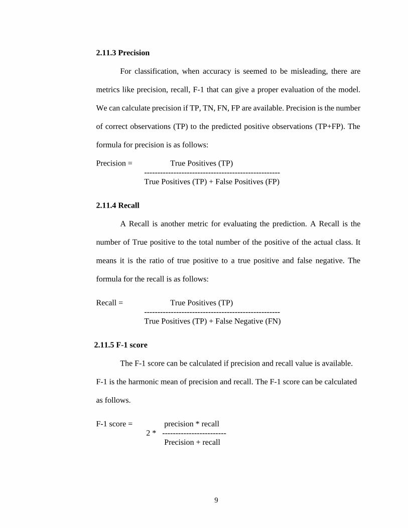
2.11.3 Precision

For classification, when accuracy is seemed to be misleading, there are

metrics like precision, recall, F-1 that can give a proper evaluation of the model.

We can calculate precision if TP, TN, FN, FP are available. Precision is the number

of correct observations (TP) to the predicted positive observations (TP+FP). The

formula for precision is as follows:

Precision = True Positives (TP)

---------------------------------------------------

True Positives (TP) + False Positives (FP)

2.11.4 Recall

A Recall is another metric for evaluating the prediction. A Recall is the

number of True positive to the total number of the positive of the actual class. It

means it is the ratio of true positive to a true positive and false negative. The

formula for the recall is as follows:

Recall = True Positives (TP)

---------------------------------------------------

True Positives (TP) + False Negative (FN)

2.11.5 F-1 score

The F-1 score can be calculated if precision and recall value is available.

F-1 is the harmonic mean of precision and recall. The F-1 score can be calculated

as follows.

F-1 score = precision * recall

2 * ------------------------

Precision + recall

10

2.12 Cross-Validation

When the model is trained using the training dataset, the model needs to be checked

if the training is correct or not if the model is not overfitted. For this reason, validation is

done. Cross-validation is done by dividing the dataset and a small portion of the dataset is

not used for training. After the training of the model is done, the remaining dataset is used

to validate the model. Such a process is known as cross-validation. There are multiple ways

for cross-validation

1. K- Fold Cross-Validation

2. Leave One Out Cross-Validation (LOOCV)’

3. Holdout

4. Repeated random sub-sampling validation

11

CHAPTER 3: STEPS OF IMPLEMENTATION

In this chapter, the steps are taken to train the model and perform the comparative

analysis are discussed.

Step 1: Gathering Data

When we use machine learning, the initial step is to know your problem. According to

problem definition, collect the data. For machine learning, you can create your dataset or

can use the one already exists. There are many platforms which provide the collection of

datasets to solve machine learning problems

Step 2: Preprocessing the data

After the data is collected, the data needs to be processed. Without preprocessing the data

or providing raw data to the model, it does not provide the expected results. Try to use the

techniques which can provide the best form of the data which increases the accuracy of the

model. If the dataset is skewed dataset try to balance it, perform feature selection, feature

extraction, transferred learning.

Step 3: Split the dataset

After cleaning data, divide the dataset. Data can be split into train test ration, train-test-

validation ratio, or use cross-validation. By splitting the dataset, you provide a training

dataset for the training of the model and remaining for evaluating the model. By doing this

we avoid the overfitting of the model.

Step 4: Choosing a model

After dealing with data, we need to select the model according to our dataset, and the type

of task needed to be performed like classification, clustering. Choosing an appropriate

model is very important or else results will not be achieved.

12

Step 5: Evaluate the model

After the training of the model, predict the results on the unseen dataset. If the prediction

metrics provide the results which are expected, then the model is said to be ready for

classifying the data. If the results are not satisfactory retrain the model and change the

parameters, fine-tune them, keep trying until the achieved results are satisfactory.

13

CHAPTER 4: METHODOLOGY

In this chapter, we are going to discuss how the results were achieved and which

methods were used to achieve the result.

4.1 About Dataset

Datasets play a very important role in Machine Learning. The efficiency of the

model depends on the type of data provided to the model. As the project includes the credit

card details as it is a credit card fraud detection task, creating a personal dataset was not

possible. So, the database used for fraud detection is from Kaggle.

Kaggle had provided the dataset that contains the transaction details or European

cardholders in September 2013. There are 31 columns in the dataset. Due to the

confidentiality issue, the dataset consists of numerical values, and columns are labeled as

V1, V2, ….., V28, Amount, Time, Class. For confidentiality, the real labels of the columns

are not provided and the whole dataset consists of numerical values as the original values

are converted into PCA values except the values of Amount and Time. The feature ‘Class’

states if the dataset instance is fraud or genuine transaction. Values for the class are either

0 or 1. 0 means Not fraud/ Genuine transaction and 1 means it is a fraudulent transaction.

There are 284807 data instances which include fraud and genuine transactions.

Figure 1 Pie Chart of dataset

14

99.827% of the dataset are genuine transactions. 0.173% of the transactions are fraudulent

transactions.

The dataset file is in CSV form. With pandas (Python library) we can read the CSV file.

Figure 2 Reading csv file of dataset

Figure 2 shows the total number of rows and columns of the dataset.

Figure 3 Rows and columns of dataset

The below figure shows the top 5 rows of the dataset, it also shows few values of

the features till V8. As seen in the figure all the values for the features are numerical values

which PCA values due to confidentiality. Time feature in the dataset is time, followed by

V1 to V28 then Amount and finally the Class.

Figure 4 Top 5 rows of the dataset

After viewing the dataset, the next step was to know how the data is distributed and

visualize the stats of data. Figure 4 shows the mean, max, in values that can be obtained by

using describe() function.

15

Figure 5 describe() for dataset

We can say that the credit card fraud dataset is highly imbalance as shown in figure

5 the number of genuine transactions is very high compared to the number of fraudulent

transactions.

Figure 6 No. of Fraud and genuine transactions

As the dataset consists of 99. 827 % of genuine transactions and only 0.173% of

fraud transactions the training with raw data will not produce expected results even if the

evaluation metrics show high results.

4.2 Classification algorithms

For the comparative analysis, the classification algorithms that are selected are

Naïve Bayes, KNN, Random Forest, Logistic Regression, and Dense Neural Network. As

we know in machine learning each parameter, hyperparameters play an important role

while training the model.

Keeping in mind, each parameter contributes differently to achieve the efficient

model, comparisons were done keeping the same parameters for all the above-listed

algorithms, and only then the results were noted. The research work done before, all the

16

researchers compared their algorithms based on the individual parameter tuning and overall

results. For this project, the comparison is done based on how each sampling technique or

feature selection works on the individual algorithm and finally tried to improve the results

of classification metrics.

Methods used to train the model using the classification algorithms are as follows

1. Using algorithms with default parameters

2. Using Standardscalar()

3. By performing feature selection

4. For all 3 sampling methods i.e. Undersampling, oversampling and SMOTE

5. Parameters tuning for each algorithm.

First comparison for all the basic models which means the parameters for the algorithms

used were by default ones.

(i) Logistic regression

The Logistic regression model was implemented using scikit-library. This library

is used for Machine Learning as it provides features for model training, data preprocessing,

model evaluation, and much more.

Figure 7 Implementing Logistic regression

The results obtained for logistic regression will be discussed in the result chapter.

The results obtained by training the logistic regression model with default parameters was

low compared to the results after applying Standardscalar() to the data. It helped in

increasing the efficiency of the model.

17

The default parameters for logistic regression were as follows:

• Penalty: It is used to set the regularization penalty.

Default value for the penalty is: l2

• Dual: It is used for dual or primal foundation

Default value: False

• Tol: it is used as a parameter for tolerance as a stopping criteria

Default: 1e-4

• C: It is used to define the inverse of regularization strength

Default: 1.0

• Random_state: int, RandomState instance, default=none: It is used as a seed number to

generate random number when it is used for shuffling of data.

• Solver: It defines the algorithm to be used for the optimization

Default: lbfgs

And more parameters can be passed in the logistic regression classifier. This classifier had

0.999 of accuracy, 0.716 for F-1 score, 0.705 for recall, 0.727 for precision for the test

dataset.

(ii) Random Forest

Random Forest classifier was implemented using the scikit-learn library.

Figure 8 Implementing Random Forest

The parameters for random forest are as follows:

• N_estimators: It defines the number of trees in the forest.

Default: 100

18

• Criterion: it is used to measure the quality of the split.

Default: Gini

• Max_depth = used to define the maximum depth of the tree.

Default: None

• N_jobs: it is used to define the number of jobs that can run in parallel

Default = None

• Verbose: Used to control the verbosity when the model is fitting or predicting

Default = 0

• Bootstrap: it is used to define whether the bootstrap samples should be used when

building the tree.

Default= True

More parameters can also be defined. Random Forest provided the best results for vanilla

model training. Accuracy for Random Forest was 0.999, Recall was 0.801, f-1 was 0.861,

precision was 0.931.

(iii) KNN

K- nearest neighbor was also defined using scikit-learn.

Figure 9 Implementing KNN

The parameters for KNN are as follows:

• N_neighbors: it defines the number of neighbors for k-neighbor.

Default: 5, used: 3 for better results

• Weights: weights are the weight function used while prediction

Default: uniform

19

• N_jobs: number of jobs that can perform parallel.

Default: None

• Metric_params: keywords for the metric function that can be added additionally

Default: None.

The results for KNN algorithms were not satisfactory. Accuracy was 1.0, precision was

0.998, recall was 0.044, F-1 was 0.084

(iv) Naïve Bayes

Naïve Bayes is implemented using scikit-learn. I have used the Gaussian Naïve

Bayes algorithm for the classification of fraud transactions.

Figure 10 Implementing Naive Bayes

The parameters for GaussuanNB was as follows:

• Priors: it is used to define the prior probabilities of the classes.

Value: n_classes

• Var_smoothing: it defines the largest variance among all the features which can be used

to add to variances for calculation stability.

Default: 1e-9

The results for Naïve Bayes were also low. Accuracy was 0.993, precision was 0.141, recall

was 0.667, F-1 was 0.232.

(v) DNN

A Dense Neural network was implemented using Keras.

The parameters for Dense Neural Network are as follows:

• Optimizer: used for optimization to minimize or maximize function and passed as a

20

parameter.

Value= adam

• Loss: loss function represents how well the dataset is provided to the model. Higher

the loss value, worse is the input to the model. If the prediction is different than actual

expected output, the loss value will be higher.

Value: binary_corssentropy

• Metrics: metrics is a function that is used to evaluate the performance of the model.

Value: accuracy

The result for DNN for accuracy was 0.990, for precision was 0.25, for recall was 0.007,

F-1 score was 0.014. The results are not satisfactory. Even the accuracy was too high, but

the other metrics were too low.

4.3 Validation of Data

After training the model, it necessary to know if the training of the model is optimal

or not. So, for that validation of data is done. There are 2 ways, train-test split or cross-

validation. For this fraud detection model evaluation, both techniques were used and both

techniques provided approximately equal accuracy value.

Figure 11 train-test split

For all the algorithms test size of kept 0.3 which means 70% of the data will be

used for training and 30% of the data will be used to evaluate the model and to predict the

class.

Creditcarddetails are the data instances for dataset features and classvalues are the class

features. By this function, the dataset instances are divided randomly into a 70-30 ratio.

21

Traun_x: values for training dataset with a class feature

Test_x: testing dataset without a class feature

Train_y: class feature values for train_x

Test_y: class feature values for Test_x

4.4 Undersampling

Undersampling was done as the dataset was highly imbalanced. The data was

randomly undersampled by reducing the number of instances of the majority class. Due to

which there are chances that few of the important data instances are not used for training

of the data. For undersampling, Random Forest performed best compared to other

algorithms.

4.5 Oversampling

Oversampling was performed as the dataset was imbalanced. The results obtained

by the models for oversampling are random sampling and SMOTE is also an oversampling

technique that was nearly similar. As oversampling increases, the number of data instances,

the training of the model is done better. The results were compared for SMOTE and random

oversampling which means with the help of the python library, the minor class instances

were randomly generated and were scattered throughout the dataset. For oversampling too

Random Forest’s performance was the best.

4.6 SMOTE

SMOTE technique is widely used for oversampling the data for the datasets that

are highly imbalanced. SMOTE technique provided better results compared to randomly

oversampling and undersampling. So, when it comes to sampling techniques for

22

classification algorithms, the SMOTE technique provides more accurate results

comparatively.

4.7 Feature Selection

For credit card fraud detection, the dataset used was having 31 features in total. One

of them was ‘class’. To improve the efficiency of the model, feature selection can be

performed, which means providing the only features to the model, which are important,

and which can be useful in training the model. Fewer features as input mean models take

less time to train the model. If only relevant features are provided as input, the efficiency

of the model can be increased. So, feature selection is important.

For the project, the feature selection was performed. Features like time, amount

were dropped as they were not correlated and were not providing any input in increasing

the accuracy of the model.

23

CHAPTER 5: RELATED WORK

Table 2 Related work

Research Paper Name

Results

Credit Card Fraud

Learning methods

Detection - Machine SMOTE technique was used to perform

credit card detection better for imbalanced

data which improve the results.

Detection of Credit Card Fraud

Transactions Using Machine Learning

Algorithms and Neural Networks: A

Comparative Study

Performed comparative analysis for

machine learning algorithms and neural

network and evaluated the best model

based on accuracy metrics.

Credit Card Fraud Detection Using

Various Classification and Sampling

Techniques: A Comparative Study

Performed a comparative analysis to

investigate among k-nearest neighbor,

logistic regression, naïve Bayes classifier,

SVM and used sampling techniques like

oversampling, undersampling, ROSE,

SMOTE.

Comparative Evaluation of credit card

fraud detection using machine learning

techniques

Comparing three algorithms i.e. Logistic

Regression, KNN, Support Vector

Machine. The evaluation is performed on

the basis on accuracy, sensitivity,

precision, specificity

24

Analysis of Machine Learning Techniques

for Credit Card Fraud Detection

Comparing ML algorithms i.e. Logistic

Regression, Random Forest, Support

Vector Machine, decision tree. The

evaluation is performed on the basis on

accuracy, sensitivity, precision, specificity

25

CHAPTER 6: RESULTS

The results for the basic models were not so satisfactory, as the dataset was highly

imbalanced. Accuracies for all the models were high as 99.8% of the data was genuine, so

accuracy mostly achieved was above 98%, but precision, recall, F-1 were low, which

means the model has not trained accurately.

In this chapter, I am going to discuss the results, achieved for the algorithms for all the

sampling methods.

• The results for vanilla for the algorithms are as follows:

Logistic regression:

Precision: 0.727, Recall: 0.705, F-1: 0.716, Accuracy: 0.999

Naïve Bayes:


KNN:


RF:


DNN:


• The results for undersampling for the algorithms are as follows:



Naïve Bayes:


26

KNN:


RF:


DNN:


• The results for oversampling for the algorithms are as follows:



Naïve Bayes:


KNN:


RF:


DNN:


• The results for SMOTE for the algorithms are as follows:



Naïve Bayes:


27

KNN:


RF:


DNN:


These were the results of all the algorithms. As seen in the results, accuracy was always

high for all the algorithms, but it is misleading, so to get better idea, I have used recall,

precision, and F-1 for comparison.

6.1 Comparing Vanilla model with the best model for all the algorithms

The difference between evaluation metrics results for vanilla model and the final

best model for all the algorithms are as follows:

1. Logistic regression:

0

0.2

0.4

0.6

0.8

1

1.2

Precision Recall F-1 Accuracy

Logistic regression

Vanilla Final

Figure 12 Logistic regression results

28

2. Naïve Bayes:

0

0.2

0.4

0.6

0.8

1

1.2


Naïve Bayes

Vanilla Final

Figure 13 Naive Bayes results

3. KNN:

0

0.2

0.4

0.6

0.8

1

1.2


KNN

Vanilla Final

Figure 14 KNN results

29

4. Random Forest:

0

0.2

0.4

0.6

0.8

1

1.2


Random Forest

Vanilla Final

Figure 15 Random Forest results

5. Dense Neural Network

0

0.2

0.4

0.6

0.8

1

1.2


Dense Neural Network

Vanilla Final

Figure 16 DNN results

30

Following are the best accuracies obtained for each algorithm using sampling methods

among which Random Forest shows the optimal results.

• Logistic regression: SMOTE (acc - 97.26%)

• Random forest: Oversampling (acc - 99.99%)

• KNN: Oversampling (acc - 99.98%)

• Naive Bayes: Oversampling (acc - 91.61%)

• Dense Neural Network: SMOTE (acc - 27.78%)

Figure 17 shows the confusion matrix for Random Forest oversampling.

Figure 17 Confusion matrix for Random Forest

31

CHAPTER 7: CONCLUSIONS AND FUTURE WORK

After comparing all the classification algorithms, it is concluded that under various

conditions, Random Forest performed best among them. After feature selection and fine-

tuning, the parameters the performance of the models was increased up to 15-20%. For

sampling method comparison, Oversampling provided best results compared to SMOTE

and undersampling. Sampling methods provided much better results compared to raw data.

Comparing all the models under every condition Random Forest performed best for

oversampling technique with 0.999 accuracy, precision, recall, and F-1 score.

For future work, the efficiency of the models can be improved if the dataset is

larger, and balanced so, that the sampling method is not needed. If the original values of

the dataset are known, then we can know how the data is correlated and which features are

really important and train accordingly. In future different methods can be used to improve

the results, more parameter tuning can be done.

32

REFERENCES

[1] Dejan Varmedja, Mirjana Karanovic, Srdjan Sladojevic, Marko Arsenovic, Andras

Anderla, “Credit Card Fraud Detection - Machine Learning methods 2019 18th

International Symposium INFOTECH-JAHORINA (INFOTECH)

[2] A. H. Nadim, I. M. Sayem, A. Mutsuddy and M. S. Chowdhury, "Analysis of Machine

Learning Techniques for Credit Card Fraud Detection," 2019 International Conference

on Machine Learning and Data Engineering (iCMLDE), Taipei, Taiwan, 2019, pp. 42-

47, doi: 10.1109/iCMLDE49015.2019.00019.

[3] I. SADGALI, N. SAEL and F. BENABBOU, "Fraud detection in credit card transaction

using machine learning techniques," 2019 1st International Conference on Smart

Systems and Data Science (ICSSD), Rabat, Morocco, 2019, pp. 1-4, doi:

10.1109/ICSSD47982.2019.9002674.

[4] O. Adepoju, J. Wosowei, S. lawte and H. Jaiman, "Comparative Evaluation of Credit

Card Fraud Detection Using Machine Learning Techniques," 2019 Global Conference

for Advancement in Technology (GCAT), BANGALURU, India, 2019, pp. 1-6, doi:

10.1109/GCAT47503.2019.8978372.

[5] J. V. V. Sriram Sasank, G. R. Sahith, K. Abhinav and M. Belwal, "Credit Card Fraud

Detection Using Various Classification and Sampling Techniques: A Comparative

Study," 2019 International Conference on Communication and Electronics Systems

(ICCES), Coimbatore, India, 2019, pp. 1713-1718, doi:

10.1109/ICCES45898.2019.9002289.

[6] D. Dighe, S. Patil and S. Kokate, "Detection of Credit Card Fraud Transactions Using

Machine Learning Algorithms and Neural Networks: A Comparative Study," 2018

https://ieeexplore-ieee-org.proxy.library.cpp.edu/author/37086837154






https://ieeexplore-ieee-org.proxy.library.cpp.edu/xpl/conhome/8713398/proceeding

https://ieeexplore-ieee-org.proxy.library.cpp.edu/xpl/conhome/8713398/proceeding

33

Fourth International Conference on Computing Communication Control and

Automation (ICCUBEA), Pune, India, 2018, pp. 1-6, doi:

10.1109/ICCUBEA.2018.8697799.

[7] S. Mittal and S. Tyagi, "Performance Evaluation of Machine Learning Algorithms for

Credit Card Fraud Detection," 2019 9th International Conference on Cloud

Computing, Data Science & Engineering (Confluence), Noida, India, 2019, pp. 320-

324, doi: 10.1109/CONFLUENCE.2019.8776925.

[8] Emailmefrom: https://www.emailmeform.com/blog/credit-card-fraud-types.html

comparing machine learning algortihms for credit card

Documents