comparing global hydrological models and combining them
TRANSCRIPT

This is an Open Access document downloaded from ORCA, Cardiff University's institutional
repository: http://orca.cf.ac.uk/129903/
This is the author’s version of a work that was submitted to / accepted for publication.
Citation for final published version:
Mehrnegar, Nooshin, Jones, Owen, Singer, Michael Bliss, Schumacher, Maike, Bates, Paul and
Forootan, Ehsan 2020. Comparing global hydrological models and combining them with GRACE
by dynamic model data averaging (DMDA). Advances in Water Resources 138 , 103528.
10.1016/j.advwatres.2020.103528 file
Publishers page: http://dx.doi.org/10.1016/j.advwatres.2020.103528
<http://dx.doi.org/10.1016/j.advwatres.2020.103528>
Please note:
Changes made as a result of publishing processes such as copy-editing, formatting and page
numbers may not be reflected in this version. For the definitive version of this publication, please
refer to the published source. You are advised to consult the publisher’s version if you wish to cite
this paper.
This version is being made available in accordance with publisher policies. See
http://orca.cf.ac.uk/policies.html for usage policies. Copyright and moral rights for publications
made available in ORCA are retained by the copyright holders.

Comparing Global Hydrological Models and Combining them1
with GRACE by Dynamic Model Data Averaging (DMDA)2
Nooshin Mehrnegara, Owen Jonesb, Michael Bliss Singera,c, Maike Schumacherd,3
Paul Batese, Ehsan Forootana,d4
aSchool of Earth and Ocean Sciences, Cardiff University, Cardiff CF103AT, UK5
bSchool of Mathematics, Cardiff University, Cardiff CF244AG, UK6
cEarth Research Institute, University of California Santa Barbara, Santa Barbara, 91306, USA7
dInstitute of Physics and Meteorology (IPM), University of Hohenheim, Stuttgart D70593,8
Germany9
eSchool of Geographical Sciences, University of Bristol, University Road, Clifton, Bristol BS81SS,10
UK11
Abstract12
Historically, hydrological models have been developed to represent land-atmosphere13
interactions by simulating water storage and water fluxes. These models, however,14
have their own unique characteristics (strength and weakness) in capturing different15
aspects of the water cycle, and their results are typically compared to or calibrated16
against in-situ observations such as river runoff measurements. As a result, there17
may be gross inaccuracies in the estimation of water storage states produced by18
these models. In this study, we present the novel approach of Dynamic Model Data19
Averaging (DMDA), which can be used to compare and merge multi-model water20
storage simulations with monthly Terrestrial Water Storage (TWS, a vertical summa-21
tion of surface and sub-surface water storage) estimates from the Gravity Recovery22
And Climate Experiment (GRACE) satellite mission. Here, the main hypothesis is23
that merging GRACE data with multi-model outputs likely provides more skillful24
hydrological estimations compared to a single model or data set. Theoretically, the25
proposed DMDA combines the benefits of the Kalman Filter (KF) and Bayesian26
Model Averaging (BMA) techniques and has the capability to deal with various ob-27
servations and models with different error structures. Based on the Bayes theory,28
DMDA provides time-variable weights for hydrological models to compute an aver-29
age of their outputs that are best fited to GRACE TWS estimates. Numerically,30
the DMDA method is implemented by integrating the output of six hydrological and31
land surface models (PCR-GLOBWB, SURFEX-TRIP, LISFLOOD, HBV-SIMREG,32
W3RA, and ORCHIDEE) and monthly GRACE TWS estimates (2002–2012) within33
the world’s 33 largest river basins, while considering the inherent uncertainties of34
1
all inputs. Our results indicate that DMDA correctly separates GRACE TWS es-35
timates into surface water, soil moisture and groundwater compartments. Linear36
trends fitted to the DMDA-derived groundwater compartment are found to be dif-37
ferent from those of original models. This means that anthropogenic influences within38
the GRACE data, which are not well reflected by models, are introduced by DMDA.39
We also find that temporal correlation coefficients between the DMDA-derived in-40
dividual water storage estimations (surface water, soil moisture, and groundwater)41
and the El Nino Southern Oscillation (ENSO) index are considerably increased com-42
pared to those derived between individual model simulations and ENSO (e.g., an43
increase from -0.2 to 0.6 in the Murray River Basin). For the Nile River Basin, they44
changed from 0.1 to 0.4 for the soil moisture, and from 0.3 to 0.7 for the surface wa-45
ter compartment. Comparisons between the DMDA-derived surface water and those46
from independent satellite altimetry observations indicate that after implementing47
DMDA, temporal correlation coefficients within major lakes are increased. Based on48
these results, we have gained confidence in the DMDA water storage estimates to be49
used for improving the characterization of water storage over broad regions of the50
globe.51
Keywords: GRACE, Terrestrial Water Storage (TWS), Dynamic Model Data52
Averaging (DMDA), Kalman Filter (KF), Bayesian Model Averaging (BMA),53
Multi-Hydrological Models, Satellite Altimetry54
1. Introduction55
Studying global water storage changes and their relationships with climate vari-56
ability and exploring their trends are important to understand the interactions be-57
tween the Earth’s water, energy, and carbon cycles. It is also essential for managing58
water resources and understanding floods and food risks in a changing climate. In-59
situ and/or remote sensing observations provide estimates of different aspects of60
the Earth system, but they do not provide water cycle closure due to sampling61
and retrieval errors. In practice, hydrological models are used to quantify hydro-62
meteorological processes such as interactions between the global climate system and63
the water cycle (Sheffield et al., 2012), the contribution of land hydrology to global64
sea level rise (Boening et al., 2012), as well as to support applications related to wa-65
ter resources planning and management (Hanington et al., 2017). However, model66
simulations are prone to errors due to imperfect model structure, as well as errors in67
inputs and forcing data that are used to run model simulations. As a result, avail-68
able models operating at regional to global scales have limited skills to reflect human69
Preprint submitted to Advances in Water Resources December 3, 2019
impacts on water storage and runoff changes (Wada et al., 2012; Scanlon et al., 2018;70
Singer et al., 2018).71
Among available remote sensing techniques, the Gravity Recovery And Climate72
Experiment (GRACE, 2002–2017) satellite mission (Tapley et al., 2004) and its73
Follow-On mission (GRACE-FO, 2018–onward) provide an opportunity to assess74
the global water cycle by monitoring time-variable gravity fields. Global GRACE-75
derived time-variable gravity field data can be used to estimate changes in Terrestrial76
Water Storage (TWS), which is a vertical summation of canopy, surface water (lakes,77
rivers, and wetlands), as well as soil moisture and groundwater storage. Changes in78
TWS provide a critical measure of regional and global water balances, which cannot79
be measured by any other satellite mission. A review of GRACE applications in80
hydrology, and particularly for groundwater monitoring, can be found in Frappart81
and Ramillien (2018).82
GRACE data can be used in conjunction with hydrological models to maximize83
information gained from modelling with rationalisation and separation of GRACE84
TWS. Thus, the gravimetric data from GRACE can inject realism into regional hy-85
drological predictions, which are often poorly constrained in terms of TWS. Generally86
speaking, integrating GRACE data with hydrological models is important from two87
perspectives: (1) it can update (modify) water storage simulation within hydrologi-88
cal models and (2) it vertically separates GRACE TWS into storage compartments.89
The first point is of interest for hydrologists since most global models are not usually90
combined with water storage observations (Bai et al., 2018). Therefore, such updates91
may lead to more realistic water storage simulations, which makes these models more92
useful for water resource applications (see e.g., Werth et al., 2009; Mostafaie et al.,93
2018). Regarding the second point, it is important to state that any attempt to94
vertically separate GRACE-derived TWS into its individual components requires a95
priori information from other sources, such as, hydrological models, satellite altime-96
try observations to estimate surface water storage, and soil moisture remote sensing97
data to estimate shallow depth soil moisture storage changes (Forootan et al., 2014).98
Various studies have developed techniques to merge multi-resources and achieve99
vertical separation of surface and sub-surface water storage compartments by several100
methods outlined below.101
(a) Forward modeling techniques are used to evaluate different compartments of102
mass variations through a simple reduction process, relying on model and/or observa-103
tion data for other compartments, e.g., surface water and soil moisture, if groundwa-104
ter should be estimated (e.g., Tiwari et al., 2009; Rodell et al., 2009; Strassberg et al.,105
2009; Feng et al., 2013; Khandu et al., 2016). This method is relatively straightfor-106
ward, but it is not necessarily the most accurate way to separate GRACE signals,107
3

due to the reflection of modeling error and/or observation errors on the final estima-108
tion of mass changes. Also, the spatial and temporal resolution of the observations109
(from satellites or in-situ) and model outputs, as well as their signal content are not110
necessarily consistent (see the discussions in, e.g., Forootan et al., 2014). Most of111
these limitations are taken into account by the methods described in what follows.112
(b) Statistical inversion techniques, which are formulated based on statistical sig-113
nal decomposition techniques, such as Principal Component Analysis (PCA, Lorenz ,114
1956) and its alternatives, e.g., Independent Component Analysis (ICA, Forootan115
and Kusche, 2012, 2013), have been used in previous studies to separate GRACE116
TWS into individual water storage estimates. For example, Schmeer et al. (2012)117
used PCA to generate a priori information about mass changes from global ocean,118
atmosphere, and land hydrology models. Then, they applied a least squares tech-119
nique to use GRACE TWS to modify their priori estimates. A statistical inversion,120
which works based on both PCA and ICA, was proposed in Forootan et al. (2014,121
2017) and Awange et al. (2014) to separate GRACE TWS using auxiliary data of sur-122
face water from satellite altimetry and individual sub-surface water storage estimate123
from a land surface model (Global Land Data Assimilation System (GLDAS, Rodell124
et al., 2004)). This inversion harmonizes the use of all available data sets within a125
single least squares framework. As a result, a more consistent mass estimate (than126
that of the forward modeling in (a)) for individual water storage components can be127
achieved.128
(c) Data Assimilation (DA) as well as simultaneous Calibration/Data Assimila-129
tion (C/DA) have been used in recent years to merge GRACE data with hydrological130
model outputs or other types of observations. These techniques rely on the model131
equations to relate water and energy fluxes to water storage changes. Therefore,132
unlike the inversion approach (b), combining information from observations (e.g.,133
GRACE TWS estimates) and a model is performed in a physically justifiable way.134
DA or C/DA can potentially increase physical understanding of the model and im-135
prove the model states by decreasing the simulation errors. For example, DA is used136
in Zaitchik et al. (2008); Girotto et al. (2016, 2017); Tian et al. (2017); Khaki et al.137
(2018d,e), while C/DA is applied in Schumacher et al. (2016, 2018) to improve global138
models such as GLDAS (Rodell et al., 2004), World-Wide Water Resources Assess-139
ment (W3RA, Van Dijk , 2010), WaterGap Global Hydrological Model (WGHM, Doll140
et al., 2003), and NOAH Multi Parameterization Land Surface Model (NOAH-MP141
LSM, Niu et al., 2011). Most of the previous DA and C/DA are implemented region-142
ally (except Van Dijk et al. (2014); Khaki et al. (2017a, 2018a)) for example over the143
Mississippi River Basin (Zaitchik et al., 2008; Schumacher et al., 2016), Bangladesh144
(Khaki et al., 2018d), the Middle East (Khaki et al., 2018e), and the Murray-Darling145
4

River Basin (Tian et al., 2017; Schumacher et al., 2018). In addition, these studies146
rely on simulation from (only) one selected hydrological model, which could contain147
errors in the model structure such as biases in the model’s internal parameters and148
boundary conditions. In each of these studies, multiple realisations of the model-149
derived water storage simulations were generated by perturbing the input forcing150
data and/or model parameters. A sequential integration techniques such as the En-151
samble Kalman Filtering (EnKF, Evensen, 1994) or its extensions was then used to152
merge GRACE data with the (ensemble) outputs of a single model (e.g., Schumacher153
et al., 2016, 2018; Khaki et al., 2017b).Van Dijk et al. (2014) used EnKF to merge154
GRACE data with a priori data from models and other remote sensing techniques.155
Their study covered the period of 2003-2012 and focused on updating the individual156
water storage estimates rather than interpreting the water storage estimates in terms157
of trends or addressing the suitability of models used to perform the analyses.158
(d) In recent years, Bayesian-based techniques have been used to combine differ-159
ent observations with models and update their outputs. For example, Long et al.160
(2017) applied the Bayesian Model Averaging (BMA, Hsu et al., 2009) technique to161
average multiple GRACE TWS products and global hydrological models to analyse162
spatial and temporal variability of global TWS. However, their study did not as-163
sess the update of individual surface and sub-surface water storage estimates. Sha164
et al. (2018) used a model-data synthesis framework based on Bayesian Hierarchical165
Modelling (BHM, see e.g., Banerjee et al., 2004) to use GRACE TWS estimates to166
update land surface deformations derived from Glacial Isostatic Adjustment (GIA)167
models. Their study did not, however, address global hydrological mass changes.168
It is worth mentioning here that the Ensamble Kalman Filter used for DA and169
C/DA can also be classified as a Bayesian-based technique because the cost function170
for updating unknown state parameters condition on the measurement data, is for-171
mulated based on the Bayes theory (see e.g., Evensen, 2003; Schumacher , 2016; Fang172
et al., 2018). Methods, such as Particle Filter (PF) and Particle Smoother (PS) are173
also Bayesian (Sarkka, 2013), and have already been applied in a wide range of geo-174
physical and hydrological applications. For example, Weerts and El Serafy (2006)175
compared the capability of EnKF and PF to update a conceptual rainfall-runoff176
model using discharge and rainfall data. Plaza Guingla et al. (2013) also used the177
standard PF to assimilate a densely sampled discharge records into a conceptual178
rainfall-runoff model. However, Bain and Crisan (2008) and Del Moral and Miclo179
(2000) show that the rate of convergence of the approximate probability distribu-180
tion until attainment of the true posterior is inversely proportional to the number181
of particles used in the filter. This means that the filter perfectly approximates the182
posterior distribution when the number of particles tends to infinity. However, since183
5

the computational cost of PF grows with the number of particles, choosing a specific184
number of particles in the design of filters is a key parameter for these methods. The185
rationale for introducing a new Bayesian data-model merging algorithm in this study186
is described in (e).187
(e) In this study, we present the Dynamic Model Data Averaging method (DMDA,188
i.e., a modified version of Dynamic Model Averaging (DMA) approach presented by189
Raftery et al., 2010) to merge multi-model derived water storage simulations with190
GRACE TWS estimates, as an alternative technique to that described in (d). Our191
main goal is to evaluate available model outputs against GRACE TWS and merge192
them in a sensible way to gain more realistic insights about global surface and sub-193
surface water storage changes. The main hypothesis behind the presented approach is194
that each global hydrological model has its own unique characteristics and strengths195
in capturing different aspects of the water cycle. Therefore, relying on a single196
model often leads to predictions that represent some phenomena or events well at197
the expenses of others. Scanlon et al. (2018) recently compared GRACE TWS with198
the outputs of global models, whose results indicated inconsistencies in long-term199
trends and cyclic (e.g., seasonal) components. Besides, many studies have concluded200
that effective combination of multiple models may provide more skillful hydrological201
simulations compared to a single model (Duan et al., 2007). Therefore, a multi-model202
choice is considered in this study.203
Our motivation to formulate the DMDA is based on its capability to deal with204
various observations and models with different structures. In summary, DMDA is205
based on the Bayes theory and provides time-variable weights to compute an average206
of hydrological model outputs, yielding the best fit to GRACE TWS estimates, while207
considering their errors (see section 3). These time-variable weights indicate which of208
the available models at a given point in time fits better to GRACE TWS estimates.209
These weights can then be used to separate the components of TWS and modify the210
estimation of water storage in these individual components. Therefore, the DMDA-211
derived ensemble is expected to yield more skillful (realistic) hydrological simulations212
compared to any individual model (see similar arguments in Duan et al., 2007). Here,213
we promote the use of DMDA over the previously introduced EnKF, PF, and PS214
methods because it is computationally more efficient in handling large dimensional215
problems such as the global integration implemented in this study. In addition, the216
DMDA’s time-variable weights can be used to assess the performance of hydrological217
models, whereas this aspect is missing in other merging techniques. More details218
about the computational aspects of DMDA are provided in section 3.219
To implement the DMDA method, surface and sub-surface water storage simu-220
lations of the six published global hydrological and land surface models (Schellekens221
6

et al., 2017) are used. These models are structurally different but they are all forced222
by the same reanalysis data set (WATCH-Forcing-Data-ERA-Interim, WFDEI Wee-223
don et al., 2014) as inputs. GRACE-derived TWS estimates are then used in the224
DMDA method to compare their outputs and merge them. A challenging problem in225
merging GRACE TWS with the outputs from multiple hydrological models is related226
to their different spatial and temporal resolutions. To overcome the computational227
problem caused by the spatial and temporal mismatch, Schumacher et al. (2016)228
introduced spatial and temporal matching functions, which are able to avoid compu-229
tational problems. In this study, we did not implement the spatial/temporal operator230
because both model outputs and GRACE data were set at monthly (temporal) and231
basin-averaged (spatial). Handling the differences in spectral domain is described232
in section 2.2. A realistic synthetic example is presented in section 4.1 to test the233
performance of the DMDA method, where the true merged values are known and the234
method can be evaluated to provide the confidence that it can be applied to a real235
case study. Our numerical results cover the world’s 33 largest river basins (see Figure236
ESM.1 in Electronic Supporting Material, ESM) for the period of 2002–2012, during237
which both GRACE data and model simulations are available. Global hydrological238
model outputs are compared against GRACE TWS, using DMDA-derived temporal239
weights, within the largest river basins for the period of this study (see section 4.2).240
The DMDA-derived updates, which are assigned to the long-term trend of surface241
and sub-surface water storage components, are explored and interpreted (see section242
4.3).243
Among many climatic factors that influence inter-annual to decadal TWS changes,244
the El Nino Southern Oscillation (ENSO, Barnston and Livezey , 1987) events rep-245
resent a dominant impact on global precipitation and TWS changes (see, e.g., Hurk-246
mans et al., 2009; Chen et al., 2010; Zhang et al., 2015; Forootan et al., 2016; Ni et al.,247
2018; Anyah et al., 2018; Forootan et al., 2019). In this study, temporal correlation248
coefficients between model-derived storage outputs and the ENSO index are used as249
a measure to determine whether implementing the DMDA helps to derive realistic250
storage simulations (see section 4.3.1). In addition, independent surface water level251
observations from satellite altimetry within14 major lakes, located in different river252
basins around the world, are used to validate our results (see section 4.4). This paper253
contains an Electronic Supporting Material (ESM) document that provide auxiliary254
information to improve understanding of the performed investigations.255
2. Data sources256
The data used in this paper include the monthly GRACE data to compute Terres-257
trial Water Storage (TWS) and individual water storage estimates from global models258
7
to provide a priori estimates to perform a Bayesian signal separation. GRACE TWS259
estimates are used in the DMDA to modify the multi-model water storage outputs.260
2.1. GRACE Data261
The latest release of the monthly GRACE level-2 (L2) product (RL06), expressed262
as dimensionless spherical harmonic coefficients up to degree and order 90, are down-263
loaded for the period of April 2002 to December 2012 from the Center for Space Re-264
search (CSR, http://www2.csr.utexas.edu/grace/RL06.html). A limited length265
of the GRACE data is used here since the global hydrological model outputs of266
Schellekens et al. (2017) were available until 2012.267
Recommended corrections are applied to generate monthly TWS fields from the268
GRACE product, i.e., degree 1 coefficients are replaced by those from Swenson et al.269
(2008) to account for the movement of the Earth’s center of mass. The zonal degree270
2 spherical harmonic coefficients (C20) are replaced by more stable ones derived from271
Satellite Laser Ranging (SLR) data (Chen et al., 2007). Surface deformations known272
as the Glacial Isostatic Adjustment (GIA) are reduced using the output of the model273
provided by Wahr and Zhong (2012). GRACE level-2’s correlated errors are reduced274
by applying the DDK2 an-isotropic de-correlation filter (Kusche et al., 2009). The275
application of smoothing filters causes a spatial leakage problem, which is evaluated276
in terms of TWS errors following the approach in Wahr et al. (1998); Khaki et al.277
(2018c) over the world’s 33 largest river basins as shown in Fig. ESM.1. An overview278
of the TWS’s strength and our error estimates is shown in ESM-section 2 (see Figure279
ESM.2).280
2.2. Global Hydrological Model (GHM) Outputs281
Monthly water balance components from six large-scale Global Hydrological Mod-282
els (GHMs) including PCR-GLOBWB (Van Beek et al., 2011; Wada et al., 2014),283
SURFEX-TRIP (Decharme et al., 2013), LISFLOOD (Van Der Knijff et al., 2010),284
HBV-SIMREG (Lindstrom et al., 1997), W3RA (Van Dijk , 2010), and ORCHIDEE285
(Polcher et al., 2011) are used in this study to provide a priori information about286
groundwater, soil moisture, surface water, canopy, and snow water storage com-287
ponents. The output of these models are published by the eartH2Observe Tier-1288
(Schellekens et al., 2017), and are available at 0.5◦ spatial resolution covering the pe-289
riod of 1979–2012 which can be downloaded from http://earth2observe.github.290
io/water-resource-reanalysis-v1.291
Although, these models are structurally different, i.e., they use different method-292
ology to simulate water changes, they are driven by the same reanalysis-based forcing293
data set, WFDEI (WATCH Forcing Data methodology applied to ERA-Interim re-294
analysis Weedon et al., 2014). In other words, all hydrological models that are used295
8

in this study may represent the TWS, but their respective approaches for simulating296
TWS and its corresponding storage compartments are not identical. For example,297
Schellekens et al. (2017) state that PCR-GLOBWB and SURFEX-TRIP contain all298
surface and sub-surface water storage components in their TWS estimation. In con-299
trast, TWS derived from LISFLOOD, HBV-SIMREG, and W3RA are equal to the300
summation of groundwater, soil moisture, and snow, while that of ORCHIDEE is301
the summation of soil moisture, surface water, and snow storage components.302
An overview of the model outputs used in this study is provided in Table 1, and303
the linear trend (as a representative of monotonic long-term storage changes) fitted304
to the model outputs are shown in ESM-section 3.305
TABLE 1
To ensure that the TWS estimates from GRACE L2 data and model outputs have306
the same spectral content, 0.5◦ resolution hydrological model outputs are transformed307
into the spectral domain and truncated to the maximum degree and order 90. The308
conversion follows an ordinary integration while considering the Gibbs effect along309
the coast lines (for more details please see, e.g., Wang et al., 2006; Forootan et al.,310
2013). Basin averages of each model components and their errors in terms of water311
storage are obtained from the same procedure used to process GRACE L2 data, i.e.,312
implemented here following Wahr et al. (1998); Khaki et al. (2018c).313
2.3. El Nino Southern Oscillation (ENSO) Index314
The El Nino Southern Oscillation (ENSO, Barnston and Livezey , 1987) is a315
large-scale inter-annual climate variability phenomenon in the Tropical Pacific Ocean,316
which affects the climate of many regions of the Earth due to its ability to change317
the global atmospheric circulation, which influences temperature and precipitation318
across the globe (Trenberth, 1990; Forootan et al., 2016). The positive phase on319
ENSO is known as El Nino, and its opposite phase is known as La Nina. The320
ENSO index used in this study is derived from sea surface temperature in the Nino321
3.4 region (5◦N − 5◦S, 170◦E − 120◦W ). Monthly ENSO index (Nino 3.4 index),322
which is provided by the NOAA National Center for Environmental Information323
(NCEI) covering 1948 onward, is downloaded from https://www.esrl.noaa.gov/324
psd/data/correlation/nina34.data. This index will be used later in this study325
to demonstrate whether the DMDA-derived surface and sub-surface water storage326
estimates are closer to the reality than those from individual models.327
2.4. Satellite Altimetry of Major Lakes328
Water level measurement by satellite altimetry has been developed and optimised329
for open oceans, yet improved post-processing techniques can be used to obtain reli-330
9

able satellite altimetry-derived height measurements within inland water bodies such331
as lakes, rivers, floodplains and wetlands (e.g., Moore and Williams , 2014; Uebbing332
et al., 2015). In this study, satellite altimetry-derived surface water observations333
are used to validate TWS changes of GRACE and models as well as surface wa-334
ter derived from GHMs and the DMDA method. Satellite altimetry time series of335
major global lakes are available from the U.S. Department of Agriculture (USDA)336
(https://ipad.fas.usda.gov/). Repeated observations of the TOPEX/Poseidon337
(T/P), Jason-1, and Jason2/OSTM altimetry missions are included in this database.338
USDA provides time series of lake water level variations from 1992 to the present-day339
within 81 lakes, and from 2008 to present-day within more than 280 lakes around340
the world. An assessment over 14 lakes located within 8 river basins of this study341
is presented in section 4.4 for the period of 2002–2012. Details of these lakes are342
reported in Table 2.343
TABLE 2
3. Dynamic Model Data Averaging (DMDA) Method344
In this section, we present the mathematical formulation of Dynamic Model Data345
Averaging (DMDA), which follows the method of Dynamic Model Averaging (DMA,346
Raftery et al., 2010) but with some modifications to achieve a recursive update of347
hydrological model outputs using GRACE TWS data (Fig. 1 summarises the DMDA348
method). It will also be shown that the implementation of DMDA combines the349
benefits of state-space merging techniques, such as Kalman Filtering (KF, Evensen,350
1994) or Particle Filtering (PF, Gordon et al., 1993), Markov Chain (MC, Metropolis351
et al., 1953; Chan and Geyer , 1994; Kuczera and Parent , 1998), and Bayesian Model352
Averaging (BMA, Hsu et al., 2009). DMDA can be applied in data assimilation353
applications that work with only one model, e.g., (Girotto et al., 2016; Khaki et al.,354
2017c,b; Schumacher et al., 2018), as well as in handling multi-model outputs as in355
Van Dijk et al. (2014).356
DMDA is formulated based on the representation of a state-space equation, which357
dynamically relates the GRACE TWS estimates and hydrological model outputs as:358
yt = ztθt + ǫt, (1)
θt = θt−1 + δt, (2)
Equation (1) is known as ‘observation equation’ and represents a linear regression359
between the observation yt (GRACE TWS estimates) and the vector of predictors360
10
zt (model-derived water storage simulations). The unknown regression parameter361
θt, commonly known as the ‘state vector’ (Bernstein, 2005), is allowed to evolve in362
time, according to equation (2), and is known as the ‘state equation’. In equations363
(1) and (2), ǫt and δt can be interpreted as the residual of output vector and state364
parameters, respectively. They are usually defined using a normal distribution with365
the mean value of zero and a standard deviation, which will be computed during the366
DMDA procedure.367
It is worth mentioning here that the EnKF (Evensen, 1994) and PF are among368
popular algorithms that can be used to recursively update an estimate of the model369
states and produce corresponding innovation values given a sequence of observations370
in the state-space equation (similar to what introduced above). In theory, EnKF371
accomplishes this goal by linear projections, and the estimations in PF are performed372
through a Sequential Monte Carlo sampling. Comparing EnKF and PF, the latter373
includes a random element so it converges to the true posterior probability function374
if the number of samples is very large. While the strength of PF is in its ability to375
account for both Gaussian and non-Gaussian error distributions, it suffers from the376
curse of dimensionality, which means that the sample size increases exponentially377
with the dimension of the state-space in order to achieve a certain performance.378
This fact precludes the use of PF in high-dimensional data-model fusion problems379
(Bengtsson et al., 2008; Daum and Huang , 2003; Snyder et al., 2008). For linear and380
Gaussian-type state-space models, as presented in this study, the PF method will381
yield the same likelihood as EnKF when the number of simulations is large enough382
(this has been tested but the results are not shown to keep the focus of this study on383
presenting the DMDA). Therefore, the DMDA, which combines the benefits of the384
EnKF and it is mathematically rigorous like PF, is adopted for the global data-model385
integration of this study.386
Equations (1) and (2) are formulated with the main assumption that there is little387
physical knowledge about how the defined regression model and its parameters are388
likely to evolve in time. However, we will show that, by introducing two parameters389
of λ and α, which are referred to as ‘forgetting factors’, one can control the temporal390
dependency of the DMDA solutions. These two parameters provide the opportunity391
to treat model simulations and observations of each step temporally dependent on,392
or independent from, previous steps. Since changes in water storage depend on the393
history of hydrological processes, accounting for temporal dependency between water394
states sounds logical.395
11

Formulating DMDA to Update Multi-Model Outputs using GRACE TWS396
Here the DMDAmethod is formulated to update the outputs of multi-hydrological397
models, Mk, (for six models: k = 1, ..., 6). It is worth mentioning that since available398
models have different storage definitions, the length of the state vector can change399
from one model to another. Additionally, the structure of each individual storage400
components can also be defined differently in different models (e.g., the number of soil401
layers does not remain constant in different hydrological models). These differences402
can be handled by DMDA.403
In the following, Yt = [y1, ..., yt] represents the vector of observations (i.e., GRACE404
TWS estimates in our study) up to the time step t. To use this vector to update the405
water storage simulation of a single-model, one can estimate the unknown (linear)406
regression parameters (θt) as407
θt−1|Yt−1 ∼ N(θt−1, Σt−1). (3)
The distribution of each parameter can be assumed to be normal with unknown408
mean θt−1 and the variance Σt−1. The regression coefficients at time t (θt) can then409
be obtained using θt−1 from equation (3) and by introducing δt ∼ N (0,Wt) to the410
state equation (equation (2)). Therefore, the desired parameters at time t are defined411
by412
θt|Yt−1 ∼ N(θt−1, Rt), (4)
where413
Rt = Σt−1 +Wt. (5)
In equation (5), Wt is the covariance matrix of the state innovation vector (δt414
in equation (2)) and it shows the dependency of the regression parameters at each415
time point to the previous time. However, in practice, there is no information about416
the temporal relationship between GRACE TWS estimates and hydrological model417
outputs to be used to define Wt. Therefore, to mathematically define a temporal418
dependency, Rt in equation (4) can be replaced by419
Rt = λ−1Σt−1, (6)
where λ (0 < λ ≤ 1) controls the influence of previous observations on the regression420
value at time t, and is known as ‘forgetting factor’ in the DMDA method (see, e.g.,421
Fagin, 1964; Jazwinski , 2007).422
Hannan et al. (1989) indicated that in the recursive estimation of auto-regressive423
models, the covariance of previous steps is derived as a weighted product of the424
12

current step (i.e., weighted by λ−1 in equation (6)). By this assumption, the effective425
window size of temporal dependency is estimated by 1/(1 − λ). In our case, we426
choose λ to be 0.95, which means that for monthly data, the effective window size is427
equivalent to 18 months. This value is chosen experimentally because it minimized428
the Root Mean Square (RMS) of differences between TWS derived from DMDA and429
GRACE.430
To apply DMDA and update water storage simulated by K different models, the431
parameter prediction of equation (4) is extended as432
θ(k)t |Mt = k, Yt−1 ∼ N(θ
(k)t−1, λ
−1Σ(k)t−1), k = 1, ..., K, (7)
where Mt = k denotes which model (from the k = 1, 2, ..., K available models)433
applies at time t, and the solution θ(k)t and Σ
(k)t−1 can be obtained using a Kalman434
Filter (KF)-type update conditional on Mt = k for each sample. This (KF-type)435
update at time t is derived as436
θ(k)t |Yt ∼ N(θ
(k)t , Σt
(k)). (8)
Regression parameters to update multi-model storage simulations can be estimated437
as438
θ(k)t = θ
(k)t−1 +R
(k)t z
(k)t (Vt + z
(k)t (R
(k)t +Q
(k)t )z
(k)Tt )T (y
(k)t − z
(k)t θ
(k)t−1), (9)
where Vt is the covariance matrix of GRACE TWS estimates (our observation), and439
Qt is the covariance matrix of predictor zt (see equation (1)). In this study, the440
leakage errors of model-derived TWS are estimated for the world’s 33 river basins441
(similar to those of GRACE). These errors are used to generate Qt, which is therefore442
a diagonal matrix in the DMDA implementation of this study. For a grid based443
implementation of DMDA, one can use the full covariance matrix of GRACE TWS444
similar to Schumacher et al. (2016). The covariance matrix Σt in equation (8) can445
be estimated from446
Σt(k) = R
(k)t −R
(k)t z
(k)Tt (Vt + z
(k)t (R
(k)t +Q
(k)t )z
(k)Tt )−1z
(k)t R
(k)t . (10)
It is evident from equations (9) and (10) that the estimation of regression parame-447
ter θt is conditional on a particular model. Therefore, the DMDA solution to obtain448
unconditional results and update multi-model simulations involves calculating the449
posterior model probability P (Mt = k|Yt) as a weight for each model, which changes450
at each time step. In the following, we show that time-variable weights need to be451
computed for each model k by choosing a forgetting factor α in a recursive method,452
13

where k = 1, ..., K. These weights are then used to average the models, which leads453
to the best fit to the GRACE TWS estimates. This justifies the term ‘Dynamic’ in454
the DMDA and makes the method different from other averaging techniques such as455
the Bayesian Model Averaging (BMA).456
Let us assume that P (Mt = k|Yt) = πt|t,k, then the posterior model probability457
for each model k at time t can be estimated as458
πt|t,k =πt|t−1,kP (yt|Mt = k, Yt−1)∑K
l=1 πt|t−1,lP (yt|Mt = l, Yt−1), (11)
where, P (yt|Mt = k, Yt−1) is the density of the observation at time t, conditional on459
model k, as well as Yt−1 = [y1, y2, ..., yt−1], which is estimated by a normal distribution460
as461
yt|Mt = k, Yt−1 ∼ N(z(k)t θ
(k)t−1, Vt + z
(k)t (R
(k)t +Q
(k)t )z
(k)Tt ), (12)
and, πt|t−1,k is the model prediction equation, which is defined by462
πt|t−1,k = ΣKl=1πt−1|t−1,kakl. (13)
In equation (12), θ(k)t−1 is estimated using the KF-type update as formulated in463
equations (9) and (10), while R(k)t is obtained from equation (6) by choosing a for-464
getting factor λ, i.e., between 0 and 1.465
In equation (13) akl = P (Mt = l|Mt−1 = k) is the element of the K×K transition466
matrix A(akl) between models, which can be onerous when the number of models is467
large, e.g., for K models and τ time steps, the number of combinations of models will468
be K2τ . In our study, we have 6 hydrological models, and 122 time steps over the469
entire period of the study (2002–2012), which leads to 6244 combinations of models.470
To specify the transition matrix A, one way is to use the Markov Chain Monte Carlo471
method (MCMC, Geyer , 2011), which will typically be computationally expensive.472
Therefore, in this study, we avoid the implicit specification of the transition matrix473
using the forgetting factor of 0 < α < 1, which has the same role as λ in equation474
(6). As a result, the model prediction equation (13) can be rewritten as475
πt|t−1,k =παt−1|t−1,k∑K
l=1 παt−1|t−1,l
. (14)
The posterior model probability, or weights, for each model at time t is estimated476
in a recursive solution between equations (11), (12), and (14). This process is initial-477
ized by setting π0|0,k =1K
for k = 1, ..., K, and assigning a prior values to the initial478
14

condition of the states θ(k)0 ∼ N(0,Σ
(k)0 ) and Σ
(k)0 =Variance (y
(k)t )/Variance (z
(k)t ).479
The reason of choosing this prior value is that in a linear regression, a regression480
coefficient for a predictor zt is likely to be less than the standard deviation of the ob-481
servations yt divided by the standard deviation of predictors zt (for more information482
see e.g., Raftery , 1993). In our numerical evaluation of DMDA with six hydrological483
models, the optimum regression estimates are found when 0.85 < α < 0.9, because484
the RMS of differences between the DMDA-derived TWS and those of GRACE were485
at a minimum here. By choosing a forgetting factor α = 0.9, we assume a tem-486
poral smoothing window with 36 month time steps between 6 hydrological model487
ensembles to predict posterior probability values of each model k at time t. It means488
that the contribution of hydrological models at time t− 37 in to the posterior model489
probability of each model k at time t is negligible. The length of this smoothing490
window is reduced e.g., to 8 months if we choose α = 0.2.491
The multi-model predictions of yt is a weighted average of model specific pre-492
diction yt, using the posterior model probabilities, πt|t,k = Pr(Mt = k|Yt), as its493
weights, i.e.,494
yDMDAt =
K∑
l=1
πt|t,ly(l)t , (15)
where y(k)t = z
(k)t θ
(k)t .495
The posterior model probability for each model at time t, along with the estimated496
time-variable regression parameter θ(k)t from KF-type updating equation (9) are used497
to estimate the multi-model prediction of water storage components as498
zDMDAj,t =
K∑
l=1
πt|t,lz(l)j,t θ
(l)j,t , (16)
where j represents each of the water storage components, i.e. groundwater, soil499
moisture, surface water, canopy, and snow. To update the water storage simulations500
of a single-model using the GRACE TWS estimates and the DMDA approach, K501
needs to be set to 1, and the prediction step is limited to the conditional estimation502
of the parameter θ(k)t |M (k)
t using equation (9).503
The posterior model probability can also be used to estimate unconditional prob-504
ability distribution of regression parameters Θt = (θ(1)t , ..., θ
(K)t ) given by observation505
Yt following506
p(Θt|Yt) =K∑
l=1
p(θ(l)t |Mt = k, Yt)P (Mt = k|Yt), (17)
15
where p(θ(k)t |M (k)
t , Yt) shows the conditional distribution of θ(k)t which is approxi-507
mated by a normal distribution as:508
θ(k)t |M (k)
t , Yt ∼ N(θ(k)t , Σ
(k)t ). (18)
The DMDA approach can be recovered to a standard Bayesian Model Averaging509
(BMA, Hoeting et al. (1999)) when α = λ = 1. Then the posterior model probability510
of model k is given by511
P (Mt = k|Yt) =p(Yt|Mt = k)
∑K
l=1 p(Yt|Mt = l), (19)
where p(Yt|Mt = k) is the marginal likelihood, obtained by integrating the product of512
the likelihood, P (Yt|θ(k),Mt = k), and the prior, P (θ(k)|Mt = k), over the parameter513
space (see also Hsu et al., 2009). Figure 1 summarises the work-flow of the DMDA514
approach.515
FIGURE 1
4. Results516
4.1. Setup a Simulation to Test the Performance of DMDA517
Before applying the DMDA method on real data, its performance is tested in a518
controlled synthetic simulation, where the results of the Bayesian update are known519
by definition. In the first step of our simulation, we aim to compare DMDA and BMA520
in terms of updating hydrological model outputs with respect to the observations (i.e.,521
GRACE TWS estimates in this study). In the second step, it will be shown that the522
DMDA-derived time-variable weights are the same as the expected values.523
To make the synthetic study simple, we assumed that TWS is defined as the524
summation of just groundwater and soil moisture components. By this definition,525
the time series of groundwater and soil moisture of two hydrological models, i.e., here526
selected as LISFLOOD (M1) and SURFEX-TRIP (M2), are introduced as predictors527
to the DMDA, and TWS derived from a third model, here selected to be PCR-528
GLOBWB, is considered as the observation (here standing in for GRACE derived529
TWS). By this choice, after applying DMDA to merge M1 and M2 with simulated530
observed TWS, we expect that the updated (DMDA-derived) groundwater and soil531
moisture storage estimates will be fitted to those of simulated observation. Here, we532
selected results within the Niger River Basin (id:20 in Fig. ESM.1), covering the pe-533
riod of 2002–2012. Figure 2 (A) shows the PCR-GLOBWB TWS as our observation,534
16

Fig. 2 (B) represents the time series of groundwater and soil moisture derived from535
M1 (B1, B3, blue curves) and M2 (B2, B4, green curves), while the expected value536
of DMDA-derived groundwater and soil moisture (simulated observation) are shown537
with the red color curves in these figures.538
The magnitude of minimum (Min), maximum (Max) and the Root Mean Square539
(RMS) of the signal for all simulated data sets can be found in Table 3. The uncer-540
tainty of these data sets are computed following a least squares error propagation,541
while considering the leakage error of GRACE TWS in the Niger River Basin. It542
is worth mentioning that the final results of the simulation do not depend on the543
selection of models and the adopted simplification. The RMS of differences between544
the simulated TWS and two selected models (reported in Table 3) indicates that M2545
(RMS of ∆TWS = 14.1 mm) had a better agreement with the observations compared546
to M1 (RMS of ∆TWS = 18.6 mm). Figure 2 (C1) shows the estimated weights for547
the first model (W1, Mean= 0.47) and second model (W2, Mean= 0.53) obtained548
using DMDA (equation (11)). These results show that the model which had a better549
agreement with observations gained higher weights.550
To compare DMDA and BMA methods to average hydrological components, we551
apply both of these methods on simulated data sets. The final results are shown in552
Fig. 2 (D1: groundwater) and (D2: soil moisture). Groundwater, soil moisture, and553
consequently TWS derived from DMDA shows better agreement with the expected554
values in comparison to the BMA results. The RMS of errors for both methods are555
reported in Table 3, which indicates that although TWS derived from BMA follow556
the expected value (RMS of error= 8.4 mm), the obtained individual components557
from this method are not close to the simulated values (RMS of errors of 20.4 mm and558
18.6 mm are found for groundwater and soil moisture, respectively). A considerable559
decrease in the differences between hydrological components and the expected values560
of DMDA shows that the method is suitable to update multi-model water storage561
estimates. Details of the numerical comparisons can be found in Table 3.562
In the second step of our simulation, we use the weights of the first step (W1, W2,563
Fig. 2 (C1)) plus a temporal white noise with standard deviation of 0.02 m (equal564
to the standard deviation of GRACE TWS error within the Niger River Basin)565
to simulate GRACE like TWS estimates. Reconstructed weights after applying the566
DMDA for the second time, using the new synthetic TWS observations, are shown in567
Fig. 2 (C2). The correlation coefficient between W1 and W2 with their reconstructed568
values is found to be 0.73 and the RMS of the reconstruction’s errors is found to be569
0.18. This indicates that the DMDA-derived weights are close to reality and further570
motivates us to apply it on real data sets.571
17

FIGURE 2572
TABLE 3
4.2. DMDA Weights to Compare Global Hydrological Models573
TWS derived from DMDA is a weighted average of selected models by estimating574
time varying weights based on the Bayes rule as in equation (15). Figure 3 shows the575
estimated weights for ten basins with the largest RMS of differences between TWS576
derived from individual models and GRACE TWS. Time-variable weights derived577
from DMDA allow us (1) to quantify the quality and compare individual water stor-578
age simulations derived from each global hydrological model against GRACE TWS579
for different periods of time, and (2) to separate GRACE TWS in a Bayesian frame-580
work, while considering different model structures and errors within and between581
model simulations and GRACE data. The average of weights during 2002–2012 is582
considered as the basis to select the best model in DMDA results over 33 river basins583
which is shown in the middle of Fig. 3. From our numerical results, PCR-GLOBWB584
is found to gain the largest weights during this period, thus, it contributed the most585
in the DMDA-derived TWS in North Asia, Central Africa, and North America.586
The weights computed for SURFEX-TRIP are found to be larger than other models587
within the snow-dominated regions, such as, the Yukon and Mackenzie in the north588
part of America and the Lena in the Northeast Asia. Our results confirm the inves-589
tigations by Schellekens et al. (2017), who compared the mentioned models against590
the Interactive Multi-sensor snow and Ice Mapping System (IMS, Ramsay , 1998).591
Apparently, multiple snow layers of SURFEX-TRIP helps it to better simulate snow592
dynamics during the cold seasons.593
We also find that SURFEX-TRIP received the highest averaged weights (com-594
pared to other models) within the Amazon and Brahmaputra River Basins during595
2002–2012. The explanation is that SURFEX-TRIP likely better accounts for (1)596
the snow coverage of the Brahmaputra River Basin, (2) the considerable contribution597
of surface water storage components in the TWS changes within the Amazon River598
Basin, and (3) the overall dry period within both basins (Chen et al., 2009; Khandu599
et al., 2016), specially the extreme hydrological droughts of 2005 and 2010 (Forootan600
et al., 2019). In the Amazon River Basin, we also find the highest performance for601
SURFEX-TRIP between 2009-2011. Chen et al. (2009) reported that in 2009 the602
Amazon River Basin experienced an extreme flood, which increased the magnitude603
of inter-annual TWS in this basin. TWS changes within the Amazon are also closely604
connected to the ENSO events in the tropical Pacific (Kousky et al., 1984; Ropelewski605
18

and Halpert , 1987). Later we will show that surface water derived from SURFEX-606
TRIP shows the highest correlation with ENSO index in comparison with the other607
models of this study. This could be another reason that we derive the highest weights608
for SURFEX-TRIP between 2009-2011 within the Amazon River Basin.609
Our results (Fig. 3) indicate that within the river basins with considerable irriga-610
tion (such as the Indus, Euphrates, and Orange River Basins), the relatively highest611
weights are assigned to the LISFLOOD and ORCHIDEE, where both account for612
human water-use (Schellekens et al., 2017). ORCHIDEE is also found to perform613
well within the Brahmaputra, Ganges, and Murray River Basins, each of which expe-614
rienced a strong decline in rainfall over the entire period of our study (e.g., 9.0 ± 4.0615
mm/decade between 1994–2014 over Ganges and Brahmaputra Khandu et al., 2016).616
Specifically, ORCHIDEE contains 14 soil layers (see Table 1) that help it to better617
resolve vertical water exchange within the irrigated regions. In ESM-section 2, it is618
shown that GRACE TWS changes within the Murray River Basin are considerably619
influenced by ENSO events (see also Forootan et al., 2012, 2016), and the simulated620
outputs of ORCHIDEE reflects these changes better than the other tested models621
justifying the higher weights that are assigned to this model within the DMDA pro-622
cedure. In ESM-section 5, we show that after applying the DMDA, model-derived623
TWS simulations are tuned to GRACE TWS.624
FIGURE 3
4.3. DMDA-Derived Individual Water Storage Estimates625
The estimated weights for the six models of section 4.2 along with the computed626
regression coefficients θt (see the flowchart of Fig. 1), are used to compute the627
DMDA-derived groundwater, soil moisture, and surface water. In order to interpret628
the monotonic changes of water storage changes within the river basins, a long-term629
linear trend is fitted to the DMDA results that are shown in Figure 4, and the630
numerical values are reported in Table 4.631
FIGURE 4632
TABLE 4
Figure 4 (a1) and (a2) show the linear trend fitted to the DMDA-derived ground-633
water and its uncertainty. The results indicate a decrease in groundwater in 42% of634
the assessed river basis (i.e., 14 of 33). The largest decreasing trends are found in635
basins with large-scale irrigation such as the Ganges (-14.77 ± 0.25 mm/yr), Indus636
(-8.26 ± 0.16 mm/yr) and Euphrates (-5.36 ± 0.23 mm/yr). The results confirm637
19

the findings by Khandu et al. (2016), Forootan et al. (2019), and Voss et al. (2013),638
respectively. The strongest increasing trends in groundwater are seen in the To-639
cantins basin (South America) at the rate of 2.41 ± 0.47 mm/yr, the Okavango640
(South Africa) with a rate of 1.74 ± 1.31 mm/yr, and the Lena (Northeast Asia)641
with 1.74 ± 0.11 mm/yr. However, all of these trends are not statistically significant.642
The positive trends in groundwater storage in these last two basins are associated643
to the heavy rainfalls, seasonal floods and the geographical location of the Okavango644
Delta (McCarthy et al., 1998), and underground ice melting caused by global warm-645
ing (Dzhamalov et al., 2012), respectively. Comparisons between the DMDA-derived646
groundwater and those of hydrological models indicate that after merging GRACE647
TWS with output from multiple hydrological models, the linear trend has changed648
considerably. This means that introducing GRACE data can successfully modify the649
anthropogenic effects, which are not well simulated by models (linear trends of the650
modelled groundwater are shown in ESM-section 3).651
The linear trend fitted to the DMDA-derived soil moisture and its uncertainty652
are shown in Fig. 4 (b1) and (b2). We find strongest increasing trends in soil653
moisture estimates within the Murray (Australia), Okavango, and Orinoco (South654
America) River Basins with rates of 6.66 ± 0.15, 3.92 ± 0.55, and 3.45 ± 0.26 mm/yr655
respectively, and largest decreasing trends in the Brahmaputra and Euphrates with656
rates of -7.00 ± 0.69 and -5.75 ± 0.39 mm/yr.657
Figure 4 (c1) and (c2) show the linear trends and their uncertainty fitted to658
the surface water storage estimated through the DMDA method. Linear trends of659
surface water within the 28 out of the 33 river basins are found to be statistically660
insignificant (values between -1 and +1 mm/yr). The strongest negative trends are661
found in the Euphrates, Murray, and Okavango River Basins with rates of -2.09 ±662
0.09, -1.47 ± 0.04, and -1.42 ± 0.37 mm/yr respectively. In contrast, the largest663
positive trends are found within the Amazon and Colorado, at the rate of 1.43 ±664
0.06 and 1.04 ± 0.04 mm/yr, respectively. The heavy flood during the summer of665
2008–2009 (Marengo et al., 2011; Chen et al., 2010), which was considerably bigger666
than the temporal mean, likely caused these positive trend in the Amazon River667
Basin. Negative trends in all three water storage compartments of the Euphrates668
River Basin (groundwater -5.36 ± 0.23 mm/yr, soil moisture -5.75 ± 0.39 mm/yr,669
and surface water -2.09 ± 0.09 mm/yr) can be associated to both irrigation and670
long-term drought as shown by Forootan et al. (2017).671
4.3.1. Contribution of ENSO in DMDA-Derived Water Storage Components672
To demonstrate that the DMDA-derived surface and sub-surface water storage673
estimates are closer to the reality than those from any individual model, we extract674
20

the dominant ENSOmode from the DMDA estimates and compare them with climate675
indices (see e.g., Anyah et al., 2018) in terms of temporal correlation coefficients with676
the ENSO index (-Nino 3.4 index, Fig. 5, 6, and 7). The reason for this comparison677
is that GRACE captures considerable variability due to the ENSO events (Phillips678
et al., 2012; Forootan et al., 2018). Therefore, by merging multi-model outputs with679
GRACE data, their skill in representing water storage changes due to large-scale680
teleconnections would be improved.681
In order to extract the ENSO modes from the DMDA-derived water storage682
estimates and the original outputs of the six models (PCRGLOB-WB, SURFEX-683
TRIP, LISFLOOD, HBV-SIMREG, W3RA, and ORCHIDEE) Principal Component684
Analysis (PCA, Lorenz , 1956) method is applied after removing the long-term linear685
trend and seasonality from hydrological components. More details about PCA results686
and extracting ENSO modes from DMDA water storage components are reported in687
ESM-section 6.688
Figure 5 shows temporal correlations between the ENSO mode of groundwater689
(from DMDA and original models) and the ENSO index. Maximum and minimum690
correlation of 0.75 and 0.53 corresponding to a maximum lag of up to 2 months are691
found globally between the DMDA groundwater and the ENSO index, respectively.692
Smaller correlations are found between the original models and the ENSO index.693
Among these models, W3RA and HBV-SIMREG indicate stronger correlations (∼694
0.6 and ∼ 0.4 respectively) with the ENSO index with a maximum lag of 2 months.695
Other models such as LISFLOOD and SURFEX-TRIP indicate notably different696
correlations (compared to HBV-SIMREG and W3RA as well as that of DMDA)697
with ENSO in various basins. We find small positive correlations with a maximum698
value of 0.3 between original PCR-GLOBWB’s groundwater and the ENSO index.699
Although the maximum lag of 3 month is estimated in most of the 33 basins, a lag700
of 15 months is estimated for the Nile, Okavango, and Zambezi (Africa), Colorado701
and Nelson (North America), Ob, Lena, and Yellow (Asia) River Basins, which are702
likely not realistic (see, e.g., Awange et al., 2014; Anyah et al., 2018).703
FIGURE 5
Similar assessments are performed between the soil moisture and surface water704
storage changes with the ENSO index and the results are shown in Figs. 6 and705
7. Correlation coefficients of up to 0.8 are computed from the DMDA estimates706
with a maximum lag of up to 2 months. Among the six models, correlation in707
soil moisture of the SURFEX-TRIP and LISFLOOD models is found to be the708
highest, i.e., correlations of 0.6 to 0.8 within the 33 river basins examined here.709
PCR-GLOBWB and W3RA show a correlation of ∼ 0.5, while those from HBV-710
21

SIMREG and ORCHIDEE are different from our other estimations, for example,711
less than 0.1 in the Niger and Nile River Basins, and greater than 0.75 in North712
Asia. Khaki et al. (2018b) indicate that over the Nile River Basin, all the three713
hydrological components, (i.e., groundwater, surface water, and soil moisture) are714
strongly influenced by ENSO. Therefore, the obtained correlation of 0.1 in the Nile715
River Basin from HBV-SIMREG is likely not realistic.716
FIGURE 6
The DMDA-derived surface water storage is compared with those of PCR-GLOBWB,717
SURFEX-TRIP, and ORCHIDEE, which contain the surface water storage compart-718
ment. The correlation coefficients are found to be generally smaller than those of soil719
moisture and groundwater components (with a maximum of 0.5), which likely shows720
that the modelling of surface water needs improvement because in reality surface wa-721
ter in lakes and rivers within regions like East Africa shows an immediate response to722
ENSO (e.g., Becker et al., 2010; Khaki et al., 2018b). Figure 7 shows that the surface723
water storage output of SURFEX-TRIP had the highest correlations with the ENSO724
index in all basins of America (values between 0.33 and 0.51) and Africa (values725
between 0.23 and 0.48), while ORCHIDEE shows the highest correlations (values726
between 0.32 and 0.58) in most parts of Asia. The correlations for PCR-GLOBWB727
are found to be relatively smaller, i.e., between 0.1 and 0.2 with lags of between 5-12728
months. Comparisons between the DMDA and original model outputs indicate that729
combining models with GRACE data improve the correlations with the ENSO index730
and the correlation lags are considerably reduced globally. It is worth mentioning731
that the DMDA results that are presented here are derived by setting the α value732
in equation (14) to 0.9. This means that we assume a 36 month temporal correla-733
tions between water storage simulations of the six models. This value guarantee an734
extraction of the ENSO modes within two PCA modes after merging GRACE and735
model outputs.736
FIGURE 7
4.4. Evaluating the DMDA Results with satellite altimetry observation737
To validate our results, TWS and surface water derived from DMDA and six738
hydrological models are compared with independent surface water observations from739
satellite altimetry. The results are shown for various regions with reliable satellite740
altimetry measurements such as the Nile, Niger, and Zambezi River Basins in Africa,741
Ob and Euphrates in Asia, St’ Lawrence and Nelson in North America, and Orinoco742
in South Africa. Here, we assessed 14 lakes located in the 8 mentioned river basins.743
22

Comparisons are performed in terms of correlation coefficients between TWS and744
surface water estimates (within the river basins), and water mass variations within745
the lakes (i.e., lake level heights from satellite altimetry data are converted to mass746
variations following Moore and Williams (2014)). The numerical results are sum-747
marized in Table 5, which indicates that after implementing the DMDA method,748
correlation coefficients are increased in most of the lakes. High values are found in749
the Nile River Basin, e.g., Tana Lake (0.718), Euphrates (Tharthar Lake, 0.569), and750
Niger (Chad Lake, 0.558), while low values are found in the Kainiji Lake of the Niger751
River Basin (0.102) and Winnipegosis of the Nelson River Basins (0.249). It should752
be noted here that although low correlations are found for some lakes, the values are753
increased when compared with the original model simulations. More details can be754
found in ESM-section 7.755
TABLE 5
5. Summary and Conclusion756
In this study, the method of Dynamic Model Data Averaging (DMDA) is intro-757
duced, which can be used (1) to compare multi-model (individual) water storage758
simulations with GRACE-derived Terrestrial Water Storage (TWS) estimates; and759
(2) to separate GRACE TWS into horological water storage compartments. DMDA760
combines the property of Kalman Filter (equations (9), (10)) and a Bayesian weight-761
ing (equation (11)) to fit multi-model water storage changes to GRACE TWS esti-762
mates. The method is flexible in accounting for errors in observations and a priori763
information (equation 9 and equation 10), and can deal with state vectors of different764
length.765
The benefit of the DMDA method over the commonly used PF or PS methods766
are twofold: 1) these methods might not be efficient for high-dimensional fusion767
tasks (e.g., Snyder et al., 2008; Van Leeuwen, 2009) such as the global hydrological768
application presented here, but the DMDA’s computational load is lower than these769
techniques; 2) DMDA provides time-variable weights that can be used to under-770
stand the behavior of a priori information (here the output of hydrological models)771
against GRACE TWS estimates, while considering their errors. The advantage of772
the DMDA over the Ensemble Kalman Filter-based of techniques is that the poste-773
rior distributions are computed through a Bayesian rule that result in more reliable774
estimations of states and their errors, while avoiding the high computational loads775
of the PF techniques.776
A realistic synthetic example was defined to evaluate the performance of DMDA777
(Fig. 2), which showed that the method is able to correctly separate GRACE TWS778
23

estimates into its individual hydrological components. We also showed that the779
DMDA’s estimation of temporal weights (for each model) was close to the real-780
ity, and can be used to assess the performance of available models. Based on the781
real data, we showed that the representation of linear trends and seasonality within782
global hydrological models, as well as their water storage changes due to the El Nino783
Southern Oscillation (ENSO) can be improved using DMDA, while considering the784
uncertainties of models and observations (see Fig. 1). Our results also showed that785
how the DMDA method is able to deal with models with different structures, and786
how it updates their water storage simulations while considering their errors. Consid-787
ering these arguments, we believe that the new water storage estimates, i.e., models788
combined with GRACE, are of great values and can be used for further hydrological789
and climate research investigations compared to model or GRACE only estimates.790
Therefore, the presented results can be considered as one step forward to improve791
model deficiencies following the insights of Scanlon et al. (2018). In what follows,792
the main conclusions and remarks of this study are summarized.793
• Estimated weights (Fig. 3) showed that the PCR-GLOBWB model gained the794
largest weights, thus, it contributed the most in the DMDA-derived TWS in795
North Asia, North America, and the center of Africa. SURFEX-TRIP per-796
formed best within basins with dominant surface water storage changes, as797
well as in snow-dominant regions. The LISFLOOD and ORCHIDEE models798
were found to perform well within irrigated basins, and those affected by ENSO799
events.800
• DMDA results in Fig. 4 (a1) showed that considerable trends exist in ground-801
water storage changes within the Ganges, Indus, and Euphrates basins during802
2002–2012. These changes are dominantly influenced by anthropogenic modi-803
fications. Trends in soil moisture (Fig. 4 (b1)) were found to be mostly related804
to meteorological prolonged drought events such as those in the Brahmaputra805
and Euphrates River Basins.806
• DMDA was able to modify the ENSO mode of water storage variability in807
most of the world’s 33 largest river basins (see Fig. 5, Fig. 6, and Fig. 7).808
DMDA assigned the biggest corrections of ENSO mode in groundwater to the809
Nile, Murray, Tocantins, Ob, Okavango and Orange River Basins. The highest810
corrections of the ENSO mode in soil moisture were found for the Nile, Niger,811
Zambezi, and Amur River Basins, and in surface water to Nile, Niger, Congo,812
Tocantins, and Murray River Basin. For example, the correlation coefficient813
between groundwater storage and ENSO in the Murray River Basin changed814
24

from -0.2 to 0.6. For the Nile River Basin, they changed from 0.1 to 0.4 for soil815
moisture, and from 0.3 to 0.7 for the surface water compartment.816
• Comparison between TWS and surface water derived from DMDA with inde-817
pendent surface water observations from satellite altimetry (Fig. ESM.15 and818
Fig. ESM.16 in ESM-section 7) showed that, DMDA was able to correctly de-819
tect the best performing model and maximize its contribution in the dynamic820
averaging process which enhanced the reality of water storage estimates.821
• To implement the DMDA in this study a forgetting factor of 0.95 was con-822
sidered in equation (6), which is equivalent to the temporal dependency in823
estimating time variable regression parameters in equation (2). In section 3,824
it was shown that this selection is equivalent to 18 months temporal depen-825
dency between GRACE TWS observations and model simulations. This value826
is selected because the DMDA results were closest to that of GRACE. After827
selecting this value, we also obtained a distinguishable ENSO mode from the828
DMDA-derived TWS and individual water storage estimates. Therefore, we829
conclude that this temporal lag might be considered in other works that at-830
tempt to apply sequential mergers or smoothers to assimilate observed water831
storage data into models.832
• In order to reduce the computational load of this work, instead of implementing833
a Markov Chain Monte Carlo (MCMC) technique to estimate the transition834
matrix between models in equation (13), a forgetting factor of 0.9 was con-835
sidered in equations (14). This might be replaced with an efficient MCMC836
implementation in future.837
The DMDA method, introduced in this study, has the potential to be used in dif-838
ferent climate and hydrological applications to compare available models (which can839
be of various types of hydrological or climate models) against reliable observations.840
It can also be used to generate ensembles from multi-model outputs such as climate841
projections. The application of this study can also be extended by incorporating842
other types of remote sensing observations such as satellite based soil moisture or843
water level data beside those of GRACE. A secondary application of the DMDA844
can also be devoted to its application for predicting (or extrapolating) water storage845
estimates. To achieve this purpose, however, the DMDA’s formulation needs to be846
extended. For example, one approach can be to use the DMDA weights, which are847
computed for the period of study, to identify best models in different river basins cov-848
ering different seasons. By analysing this information and knowing the TWS in the849
25

future, one can use a combination of different model runs (weighted by the DMDA850
outputs) and extrapolate the surface and sub-surface water storage estimates.851
26
References852
Anyah, R. O., E. Forootan, J. L. Awange, and M. Khaki (2018), Understanding853
linkages between global climate indices and terrestrial water storage changes over854
africa using grace products, Science of The Total Environment, 635, 1405–1416,855
doi:10.1016/j.scitotenv.2018.04.159.856
Awange, J. L., E. Forootan, M. Kuhn, J. Kusche, and B. Heck (2014), Water stor-857
age changes and climate variability within the nile basin between 2002 and 2011,858
Advances in Water Resources, 73, 1–15, doi:10.1016/j.advwatres.2014.06.010.859
Bai, P., X. Liu, and C. Liu (2018), Improving hydrological simulations by incor-860
porating grace data for model calibration, Journal of Hydrology, 557, 291–304,861
doi:10.1016/j.jhydrol.2017.12.025.862
Bain, A., and D. Crisan (2008), Fundamentals of stochastic filtering, vol. 60, Springer863
Science & Business Media, doi:10.1007/978-0-387-76896-0.864
Banerjee, S., B. P. Carlin, and A. E. Gelfand (2004), Hierarchical modeling and865
analysis for spatial data, Chapman and Hall/CRC.866
Barnston, A. G., and R. E. Livezey (1987), Classification, seasonality and persistence867
of low-frequency atmospheric circulation patterns,Monthly weather review, 115 (6),868
1083–1126, doi:10.1175/1520-0493(1987)115〈1083:CSAPOL〉2.0.CO;2.869
Becker, M., W. LLovel, A. Cazenave, A. Guntner, and J.-F. Cretaux (2010), Recent870
hydrological behavior of the east african great lakes region inferred from grace,871
satellite altimetry and rainfall observations, Comptes Rendus Geoscience, 342 (3),872
223–233, doi:10.1016/j.crte.2009.12.010.873
Bengtsson, T., P. Bickel, B. Li, et al. (2008), Curse-of-dimensionality revisited: Col-874
lapse of the particle filter in very large scale systems, in Probability and statistics:875
Essays in honor of David A. Freedman, pp. 316–334, Institute of Mathematical876
Statistics, doi:10.1214/193940307000000518.877
Bernstein, D. S. (2005), Matrix mathematics: Theory, facts, and formulas with ap-878
plication to linear systems theory, vol. 41, Princeton university press Princeton.879
Boening, C., J. K. Willis, F. W. Landerer, R. S. Nerem, and J. Fasullo (2012), The880
2011 la nina: So strong, the oceans fell, Geophysical Research Letters, 39 (19),881
doi:10.1029/2012GL053055.882
27

Chan, K. S., and C. J. Geyer (1994), Discussion: Markov chains for explor-883
ing posterior distributions, The Annals of Statistics, 22 (4), 1747–1758, doi:884
10.1214/aos/1176325754.885
Chen, J. L., C. R. Wilson, J. S. Famiglietti, and M. Rodell (2007), Attenuation effect886
on seasonal basin-scale water storage changes from grace time-variable gravity,887
Journal of Geodesy, 81 (4), 237–245, doi:10.1007/s00190-006-0104-2.888
Chen, J. L., C. R. Wilson, B. D. Tapley, Z. L. Yang, and G. Y. Niu (2009), 2005889
drought event in the amazon river basin as measured by grace and estimated890
by climate models, Journal of Geophysical Research: Solid Earth, 114 (B5), doi:891
10.1029/2008JB006056.892
Chen, J. L., C. R. Wilson, and B. D. Tapley (2010), The 2009 exceptional amazon893
flood and interannual terrestrial water storage change observed by grace, Water894
Resources Research, 46 (12), doi:10.1029/2010WR009383.895
Daum, F., and J. Huang (2003), Curse of dimensionality and particle filters, in 2003896
IEEE Aerospace Conference Proceedings (Cat. No. 03TH8652), vol. 4, pp. 4 1979–897
4 1993, IEEE, doi:10.1109/AERO.2003.1235126.898
Decharme, B., E. Martin, and S. Faroux (2013), Reconciling soil thermal and hydro-899
logical lower boundary conditions in land surface models, Journal of Geophysical900
Research: Atmospheres, 118 (14), 7819–7834, doi:10.1002/jgrd.50631.901
Del Moral, P., and L. Miclo (2000), Branching and interacting particle systems ap-902
proximations of feynman-kac formulae with applications to non-linear filtering, in903
Seminaire de probabilites XXXIV, pp. 1–145, Springer, doi:10.1007/BFb0103798.904
Doll, P., F. Kaspar, and B. Lehner (2003), A global hydrological model for deriving905
water availability indicators: model tuning and validation, Journal of Hydrology,906
270 (1-2), 105–134, doi:10.1016/S0022-1694(02)00283-4.907
Duan, Q., N. K. Ajami, X. Gao, and S. Sorooshian (2007), Multi-model ensemble hy-908
drologic prediction using bayesian model averaging, Advances in Water Resources,909
30 (5), 1371–1386, doi:10.1016/j.advwatres.2006.11.014.910
Dzhamalov, R. G., G. N. Krichevets, and T. I. Safronova (2012), Current changes in911
water resources in lena river basin, Water Resources, 39 (2), 147–160, doi:10.1134/912
S0097807812020042.913
28

Evensen, G. (1994), Sequential data assimilation with a nonlinear quasi-geostrophic914
model using monte carlo methods to forecast error statistics, Journal of Geophys-915
ical Research: Oceans, 99 (C5), 10,143–10,162, doi:10.1029/94JC00572.916
Evensen, G. (2003), The ensemble kalman filter: Theoretical formulation917
and practical implementation, Ocean dynamics, 53 (4), 343–367, doi:10.1007/918
s10236-003-0036-9.919
Fagin, S. L. (1964), Recursive linear regression theory, optimal filter theory, and error920
analysis of optimal systems, in IEEE international convention record, vol. 12, pp.921
216–245.922
Fang, H., N. Tian, Y. Wang, M. Zhou, and M. A. Haile (2018), Nonlinear bayesian923
estimation: from kalman filtering to a broader horizon, IEEE/CAA Journal of924
Automatica Sinica, 5 (2), 401–417, doi:10.1109/JAS.2017.7510808.925
Feng, W., M. Zhong, J. M. Lemoine, R. Biancale, H.-T. Hsu, and J. Xia (2013),926
Evaluation of groundwater depletion in north china using the gravity recovery927
and climate experiment (grace) data and ground-based measurements, Water Re-928
sources Research, 49 (4), 2110–2118, doi:10.1002/wrcr.20192.929
Forootan, E., and J. Kusche (2012), Separation of global time-variable gravity signals930
into maximally independent components, Journal of Geodesy, 86 (7), 477–497, doi:931
0.1007/s00190-011-0532-5.932
Forootan, E., and J. Kusche (2013), Separation of deterministic signals using inde-933
pendent component analysis (ica), Studia Geophysica et Geodaetica, 57 (1), 17–26,934
doi:10.1007/s11200-012-0718-1.935
Forootan, E., J. Awange, J. Kusche, B. Heck, and A. Eicker (2012), Independent936
patterns of water mass anomalies over australia from satellite data and models,937
Remote sensing of environment, 124, 427–443, doi:10.1016/j.rse.2012.05.023.938
Forootan, E., O. Didova, J. Kusche, and A. Locher (2013), Comparisons of atmo-939
spheric data and reduction methods for the analysis of satellite gravimetry ob-940
servations, Journal of Geophysical Research: Solid Earth, 118 (5), 2382–2396, doi:941
10.1002/jgrb.50160.942
Forootan, E., R. Rietbroek, J. Kusche, M. A. Sharifi, J. L. Awange, M. Schmidt,943
P. Omondi, and J. S. Famiglietti (2014), Separation of large scale water storage944
patterns over iran using grace, altimetry and hydrological data, Remote Sensing945
of Environment, 140, 580–595, doi:10.1016/j.rse.2013.09.025.946
29

Forootan, E., J. L. Awange, M. Schumacher, R. O. Anyah, A. I. J. M. van Dijk,947
J. Kusche, et al. (2016), Quantifying the impacts of enso and iod on rain gauge948
and remotely sensed precipitation products over australia, Remote sensing of En-949
vironment, 172, 50–66, doi:10.1016/j.rse.2015.10.027.950
Forootan, E., A. Safari, A. Mostafaie, M. Schumacher, M. Delavar, and J. L. Awange951
(2017), Large-scale total water storage and water flux changes over the arid and952
semiarid parts of the middle east from grace and reanalysis products, Surveys in953
Geophysics, 38 (3), 591–615, doi:10.1007/s10712-016-9403-1.954
Forootan, E., J. Kusche, M. Talpe, C. K. Shum, and M. Schmidt (2018), Develop-955
ing a complex independent component analysis (cica) technique to extract non-956
stationary patterns from geophysical time series, Surveys in Geophysics, 39 (3),957
435–465, doi:10.1007/s10712-017-9451-1.958
Forootan, E., M. Khaki, M. Schumacher, V. Wulfmeyer, N. Mehrnegar, A. I. J. M.959
van Dijk, L. Brocca, S. Farzaneh, F. Akinluyi, G. Ramillien, C. Shum, J. L.960
Awange, and A. Mostafaie (2019), Understanding the global hydrological droughts961
of 2003–2016 and their relationships with teleconnections, Science of The Total962
Environment, 650, 2587–2604, doi:10.1016/j.scitotenv.2018.09.231.963
Frappart, F., and G. Ramillien (2018), Monitoring groundwater storage changes964
using the gravity recovery and climate experiment (grace) satellite mission: A965
review, Remote Sensing, 10 (6), 829, doi:10.3390/rs10060829.966
Geyer, C. J. (2011), Introduction to markov chain monte carlo, Handbook of Markov967
Chain Monte Carlo, p. 46.968
Girotto, M., G. J. De Lannoy, R. H. Reichle, and M. Rodell (2016), Assimilation of969
gridded terrestrial water storage observations from grace into a land surface model,970
Water Resources Research, 52 (5), 4164–4183, doi:10.1002/2015WR018417.971
Girotto, M., G. J. De Lannoy, R. H. Reichle, M. Rodell, C. Draper, S. N. Bhanja,972
and A. Mukherjee (2017), Benefits and pitfalls of grace data assimilation: A case973
study of terrestrial water storage depletion in india, Geophysical research letters,974
44 (9), 4107–4115, doi:10.1002/2017GL072994.975
Gordon, N. J., D. J. Salmond, and A. F. Smith (1993), Novel approach to976
nonlinear/non-gaussian bayesian state estimation, in IEE proceedings F (radar977
and signal processing), vol. 140, pp. 107–113, IET, doi:10.1049/ip-f-2.1993.0015.978
30

Hanington, P., Q. T. To, P. D. T. Van, N. A. V. Doan, and A. S. Kiem (2017), A979
hydrological model for interprovincial water resource planning and management:980
a case study in the long xuyen quadrangle, mekong delta, vietnam, Journal of981
Hydrology, 547, 1–9, doi:10.1016/j.jhydrol.2017.01.030.982
Hannan, E. J., A. McDougall, and D. Poskitt (1989), Recursive estimation of au-983
toregressions, Journal of the Royal Statistical Society. Series B (Methodological),984
51 (2), 217–233, doi:10.1111/j.2517-6161.1989.tb01759.x.985
Hoeting, J. A., D. Madigan, A. E. Raftery, and C. T. Volinsky (1999), Bayesian986
model averaging: A tutorial, Statistical Science, 14 (4), 382–417.987
Hsu, K.-l., H. Moradkhani, and S. Sorooshian (2009), A sequential bayesian approach988
for hydrologic model selection and prediction, Water Resources Research, 45 (12),989
doi:10.1029/2008WR006824.990
Hurkmans, R., P. A. Troch, R. Uijlenhoet, P. Torfs, and M. Durcik (2009), Effects991
of climate variability on water storage in the colorado river basin, Journal of992
hydrometeorology, 10 (5), 1257–1270, doi:10.1175/2009JHM1133.1.993
Jazwinski, A. H. (2007), Stochastic processes and filtering theory, Courier Corpora-994
tion.995
Khaki, M., B. Ait-El-Fquih, I. Hoteit, E. Forootan, J.L., and M. Kuhn (2017a), A996
two-update ensemble kalman filter for land hydrological data assimilation with an997
uncertain constraint, Journal of Hydrology, 555, 447–462, doi:10.1016/j.jhydrol.998
2017.10.032.999
Khaki, M., I. Hoteit, M. Kuhn, J. L. Awange, E. Forootan, A. I. J. M. Van Dijk,1000
M. Schumacher, and C. Pattiaratchi (2017b), Assessing sequential data assimila-1001
tion techniques for integrating grace data into a hydrological model, Advances in1002
Water Resources, 107, 301–316, doi:10.1016/j.advwatres.2017.07.001.1003
Khaki, M., M. Schumacher, E. Forootan, M. Kuhn, J. L. Awange, and A. I. J. M.1004
van Dijk (2017c), Accounting for spatial correlation errors in the assimilation of1005
grace into hydrological models through localization, Advances in Water Resources,1006
108, 99–112, doi:10.1016/j.advwatres.2017.07.024.1007
Khaki, M., B. Ait-El-Fquih, I. Hoteit, E. Forootan, J. L. Awange, and M. Kuhn1008
(2018a), Unsupervised ensemble kalman filtering with an uncertain constraint for1009
land hydrological data assimilation, Journal of Hydrology, 564, 175–190, doi:10.1010
1016/j.jhydrol.2018.06.080.1011
31

Khaki, M., J. L. Awange, E. Forootan, and M. Kuhn (2018b), Understanding the1012
association between climate variability and the nile’s water level fluctuations and1013
water storage changes during 1992–2016, Science of The Total Environment, 645,1014
1509–1521, doi:10.1016/j.scitotenv.2018.07.212.1015
Khaki, M., E. Forootan, M. Kuhn, J. L. Awange, L. Longuevergne, and Y. Wada1016
(2018c), Efficient basin scale filtering of grace satellite products, Remote Sensing1017
of Environment, 204, 76–93, doi:10.1016/j.rse.2017.10.040.1018
Khaki, M., E. Forootan, M. Kuhn, J. L. Awange, F. Papa, and C. K. Shum (2018d),1019
A study of bangladesh’s sub-surface water storages using satellite products and1020
data assimilation scheme, Science of the Total Environment, 625, 963–977, doi:1021
10.1016/j.scitotenv.2017.12.289.1022
Khaki, M., E. Forootan, M. Kuhn, J. L. Awange, A. I. J. M. van Dijk, M. Schu-1023
macher, and M. A. Sharifi (2018e), Determining water storage depletion within1024
iran by assimilating grace data into the w3ra hydrological model, Advances in1025
Water Resources, 114, 1–18, doi:10.1016/j.advwatres.2018.02.008.1026
Khandu, K., E. Forootan, M. Schumacher, J. L. Awange, and H. Muller-Schmied1027
(2016), Exploring the influence of precipitation extremes and human water use on1028
total water storage (tws) changes in the ganges-brahmaputra-meghna river basin,1029
Water Resources Research, 52 (3), 2240–2258, doi:10.1002/2015WR018113.1030
Kousky, V. E., M. T. Kagano, and I. F. Cavalcanti (1984), A review of the southern1031
oscillation: oceanic-atmospheric circulation changes and related rainfall anomalies,1032
Tellus A, 36 (5), 490–504, doi:10.1111/j.1600-0870.1984.tb00264.x.1033
Kuczera, G., and E. Parent (1998), Monte carlo assessment of parameter uncertainty1034
in conceptual catchment models: the metropolis algorithm, Journal of Hydrology,1035
211 (1-4), 69–85, doi:10.1016/S0022-1694(98)00198-X.1036
Kusche, J., R. Schmidt, S. Petrovic, and R. Rietbroek (2009), Decorrelated grace1037
time-variable gravity solutions by gfz, and their validation using a hydrological1038
model, Journal of geodesy, 83 (10), 903–913, doi:10.1007/s00190-009-0308-3.1039
Lindstrom, G., B. Johansson, M. Persson, M. Gardelin, and S. Bergstrom (1997),1040
Development and test of the distributed hbv-96 hydrological model, Journal of1041
hydrology, 201 (1-4), 272–288, doi:10.1016/S0022-1694(97)00041-3.1042
32

Long, D., Y. Pan, J. Zhou, Y. Chen, X. Hou, Y. Hong, B. R. Scanlon, and L. Longuev-1043
ergne (2017), Global analysis of spatiotemporal variability in merged total water1044
storage changes using multiple grace products and global hydrological models,1045
Remote sensing of environment, 192, 198–216, doi:10.1016/j.rse.2017.02.011.1046
Lorenz, E. N. (1956), Empirical orthogonal functions and statistical weather predic-1047
tion.1048
Marengo, J. A., C. A. Nobre, G. Sampaio, L. F. Salazar, and L. S. Borma (2011),1049
Climate change in the amazon basin: Tipping points, changes in extremes, and1050
impacts on natural and human systems, in Tropical rainforest responses to climatic1051
change, pp. 259–283, Springer, doi:10.1007/978-3-642-05383-2 9.1052
McCarthy, T. S., A. Bloem, and P. A. Larkin (1998), Observations on the hydrology1053
and geohydrology of the okavango delta, South African Journal of Geology/Suid-1054
Afrikaanse Tydskrif vir Geologie, 101 (2), 101–117.1055
Metropolis, N., A. W. Rosenbluth, M. N. Rosenbluth, A. H. Teller, and E. Teller1056
(1953), Equation of state calculations by fast computing machines, The journal of1057
chemical physics, 21 (6), 1087–1092, doi:10.1063/1.1699114.1058
Moore, P., and S. D. P. Williams (2014), Integration of altimetric lake levels and grace1059
gravimetry over africa: Inferences for terrestrial water storage change 2003–2011,1060
Water Resources Research, 50 (12), 9696–9720, doi:10.1002/2014WR015506.1061
Mostafaie, A., E. Forootan, A. Safari, and M. Schumacher (2018), Comparing multi-1062
objective optimization techniques to calibrate a conceptual hydrological model1063
using in situ runoff and daily grace data, Computational Geosciences, 22 (3), 789–1064
814, doi:10.1007/s10596-018-9726-8.1065
Ni, S., J. Chen, C. R. Wilson, J. Li, X. Hu, and R. Fu (2018), Global terrestrial water1066
storage changes and connections to enso events, Surveys in Geophysics, 39 (1), 1–1067
22, doi:10.1007/s10712-017-9421-7.1068
Niu, G.-Y., Z.-L. Yang, K. E. Mitchell, F. Chen, M. B. Ek, M. Barlage, A. Kumar,1069
K. Manning, D. Niyogi, E. Rosero, et al. (2011), The community noah land sur-1070
face model with multiparameterization options (noah-mp): 1. model description1071
and evaluation with local-scale measurements, Journal of Geophysical Research:1072
Atmospheres, 116 (D12), doi:10.1029/2010JD015139.1073
33

Phillips, T., R. Nerem, B. Fox-Kemper, J. Famiglietti, and B. Rajagopalan (2012),1074
The influence of enso on global terrestrial water storage using grace, Geophysical1075
Research Letters, 39 (16), doi:10.1029/2012GL052495.1076
Plaza Guingla, D. A., R. De Keyser, G. J. De Lannoy, L. Giustarini, P. Matgen, and1077
V. R. Pauwels (2013), Improving particle filters in rainfall-runoff models: Appli-1078
cation of the resample-move step and the ensemble gaussian particle filter, Water1079
Resources Research, 49 (7), 4005–4021, doi:10.1002/wrcr.20291.1080
Polcher, J., N. Bertrand, H. Biemans, D. B. Clark, M. Floerke, N. Gedney, D. Gerten,1081
T. Stacke, M. Van Vliet, and F. Voss (2011), Improvements in hydrological pro-1082
cesses in general hydrological models and land surface models within watch.1083
Raftery, A. (1993), Model selection and accounting for model uncertainty in linear1084
regression models, Citeseer.1085
Raftery, A. E., M. Karny, and P. Ettler (2010), Online prediction under model1086
uncertainty via dynamic model averaging: Application to a cold rolling mill, Tech-1087
nometrics, 52 (1), 52–66, doi:10.1198/TECH.2009.08104.1088
Ramsay, B. H. (1998), The interactive multisensor snow and ice mapping system, Hy-1089
drological Processes, 12 (10-11), 1537–1546, doi:10.1002/(SICI)1099-1085(199808/1090
09)12:10/11〈1537::AID-HYP679〉3.0.CO;2-A.1091
Rodell, M., P. R. Houser, U. Jambor, J. Gottschalck, K. Mitchell, C.-J. Meng, K. Ar-1092
senault, B. Cosgrove, J. Radakovich, M. Bosilovich, et al. (2004), The global land1093
data assimilation system, Bulletin of the American Meteorological Society, 85 (3),1094
381–394, doi:10.1175/BAMS-85-3-381.1095
Rodell, M., I. Velicogna, and J. S. Famiglietti (2009), Satellite-based estimates of1096
groundwater depletion in india, Nature, 460 (7258), 999, doi:10.1038/nature08238.1097
Ropelewski, C. F., and M. S. Halpert (1987), Global and regional scale precipitation1098
patterns associated with the el nino/southern oscillation, Monthly weather review,1099
115 (8), 1606–1626, doi:10.1175/1520-0493(1987)115〈1606:GARSPP〉2.0.CO;2.1100
Sarkka, S. (2013), Bayesian filtering and smoothing, vol. 3, Cambridge University1101
Press, doi:10.1201/b16018.1102
Scanlon, B. R., Z. Zhang, H. Save, A. Y. Sun, H. M. Schmied, L. P. van Beek, D. N.1103
Wiese, Y. Wada, D. Long, R. C. Reedy, et al. (2018), Global models underestimate1104
34
large decadal declining and rising water storage trends relative to grace satellite1105
data, Proceedings of the National Academy of Sciences, 115 (6), E1080–E1089,1106
doi:10.1073/pnas.1704665115.1107
Schellekens, J., E. Dutra, A. Martınez-de la Torre, G. Balsamo, A. van Dijk, F. S.1108
Weiland, M. Minvielle, J.-C. Calvet, B. Decharme, S. Eisner, et al. (2017), A global1109
water resources ensemble of hydrological models: the earth2observe tier-1 dataset,1110
Earth System Science Data, 9 (2), 389–413, doi:10.5194/essd-9-389-2017.1111
Schmeer, M., M. Schmidt, W. Bosch, and F. Seitz (2012), Separation of mass sig-1112
nals within grace monthly gravity field models by means of empirical orthogonal1113
functions, Journal of Geodynamics, 59, 124–132, doi:10.1016/j.jog.2012.03.001.1114
Schumacher, M. (2016), Methods for assimilating remotely-sensed water storage1115
changes into hydrological models, Ph.D. thesis, Universitats-und Landesbibliothek1116
Bonn.1117
Schumacher, M., J. Kusche, and P. Doll (2016), A systematic impact assessment1118
of grace error correlation on data assimilation in hydrological models, Journal of1119
Geodesy, 90 (6), 537–559, doi:10.1007/s00190-016-0892-y.1120
Schumacher, M., E. Forootan, A. I. J. M. van Dijk, H. M. Schmied, R. S. Crosbie,1121
J. Kusche, and P. Doll (2018), Improving drought simulations within the murray-1122
darling basin by combined calibration/assimilation of grace data into the watergap1123
global hydrology model, Remote Sensing of Environment, 204, 212–228, doi:10.1124
1016/j.rse.2017.10.029.1125
Sha, Z., J. Rougier, M. Schumacher, and J. Bamber (2018), Bayesian model-data1126
synthesis with an application to global glacio-isostatic adjustment, Environmetrics,1127
doi:10.1002/env.2530.1128
Sheffield, J., E. F. Wood, and M. L. Roderick (2012), Little change in global drought1129
over the past 60 years, Nature, 491 (7424), 435, doi:10.1038/nature11575.1130
Singer, M. B., K. Michaelides, and D. E. Hobley (2018), Storm 1.0: a simple,1131
flexible, and parsimonious stochastic rainfall generator for simulating climate1132
and climate change, Geoscientific Model Development, 11 (9), 3713–3726, doi:1133
10.5194/gmd-11-3713-2018.1134
Snyder, C., T. Bengtsson, P. Bickel, and J. Anderson (2008), Obstacles to high-1135
dimensional particle filtering, Monthly Weather Review, 136 (12), 4629–4640, doi:1136
10.1175/2008MWR2529.1.1137
35

Strassberg, G., B. R. Scanlon, and D. Chambers (2009), Evaluation of groundwa-1138
ter storage monitoring with the grace satellite: Case study of the high plains1139
aquifer, central united states, Water Resources Research, 45 (5), doi:10.1029/1140
2008WR006892.1141
Swenson, S., D. Chambers, and J. Wahr (2008), Estimating geocenter variations from1142
a combination of grace and ocean model output, Journal of Geophysical Research:1143
Solid Earth, 113 (B8), doi:10.1029/2007JB005338.1144
Tapley, B. D., S. Bettadpur, J. C. Ries, P. F. Thompson, and M. M. Watkins (2004),1145
Grace measurements of mass variability in the earth system, Science, 305 (5683),1146
503–505, doi:10.1126/science.1099192.1147
Tian, S., P. Tregoning, L. J. Renzullo, A. I. J. M. van Dijk, J. P. Walker, V. R.1148
Pauwels, and S. Allgeyer (2017), Improved water balance component estimates1149
through joint assimilation of grace water storage and smos soil moisture retrievals,1150
Water Resources Research, 53 (3), 1820–1840, doi:10.1002/2016WR019641.1151
Tiwari, V., J. Wahr, and S. Swenson (2009), Dwindling groundwater resources in1152
northern india, from satellite gravity observations, Geophysical Research Letters,1153
36 (18), doi:10.1029/2009GL039401.1154
Trenberth, K. E. (1990), Recent observed interdecadal climate changes in the north-1155
ern hemisphere, Bulletin of the American Meteorological Society, 71 (7), 988–993,1156
doi:10.1175/1520-0477(1990)071〈0988:ROICCI〉2.0.CO;2.1157
Uebbing, B., J. Kusche, and E. Forootan (2015), Waveform retracking for improving1158
level estimations from topex/poseidon, jason-1, and jason-2 altimetry observations1159
over african lakes, IEEE Transactions on Geoscience and Remote Sensing, 53 (4),1160
2211–2224, doi:10.1109/TGRS.2014.2357893.1161
Van Beek, L. P. H., Y. Wada, and M. F. P. Bierkens (2011), Global monthly water1162
stress: 1. water balance and water availability, Water Resources Research, 47 (7),1163
doi:10.1029/2010WR009791.1164
Van Der Knijff, J. M., J. Younis, and A. P. J. De Roo (2010), Lisflood: a gis-1165
based distributed model for river basin scale water balance and flood simulation,1166
International Journal of Geographical Information Science, 24 (2), 189–212, doi:1167
10.1080/13658810802549154.1168
36

Van Dijk, A. I. J. M. (2010), The australian water resources assessment system:1169
Technical 901 report 3, landscape model (version 0.5) technical description, csiro,1170
Water for a Healthy Country National Research Flagship.1171
Van Dijk, A. I. J. M., L. J. Renzullo, Y. Wada, and P. Tregoning (2014), A global1172
water cycle reanalysis (2003–2012) merging satellite gravimetry and altimetry ob-1173
servations with a hydrological multi-model ensemble, Hydrology and Earth System1174
Sciences, 18 (8), 2955–2973, doi:10.5194/hess-18-2955-2014.1175
Van Leeuwen, P. J. (2009), Particle filtering in geophysical systems, Monthly Weather1176
Review, 137 (12), 4089–4114, doi:10.1175/2009MWR2835.1.1177
Voss, K. A., J. S. Famiglietti, M. Lo, C. De Linage, M. Rodell, and S. C. Swenson1178
(2013), Groundwater depletion in the middle east from grace with implications1179
for transboundary water management in the tigris-euphrates-western iran region,1180
Water resources research, 49 (2), 904–914, doi:10.1002/wrcr.20078.1181
Wada, Y., L. P. H. van Beek, F. C. S. Weiland, B. F. Chao, Y.-H. Wu, and M. F. P.1182
Bierkens (2012), Past and future contribution of global groundwater depletion to1183
sea-level rise, Geophysical Research Letters, 39 (9), doi:10.1029/2012GL051230.1184
Wada, Y., D. Wisser, and M. Bierkens (2014), Global modeling of withdrawal, al-1185
location and consumptive use of surface water and groundwater resources, Earth1186
System Dynamics Discussions, 5 (1), 15–40, doi:10.5194/esdd-4-355-2013.1187
Wahr, J., and S. Zhong (2012), Computations of the viscoelastic response of a 3-d1188
compressible earth to surface loading: an application to glacial isostatic adjustment1189
in antarctica and canada, Geophysical Journal International, 192 (2), 557–572, doi:1190
10.1093/gji/ggs030.1191
Wahr, J., M. Molenaar, and F. Bryan (1998), Time variability of the earth’s gravity1192
field: Hydrological and oceanic effects and their possible detection using grace,1193
Journal of Geophysical Research: Solid Earth, 103 (B12), 30,205–30,229, doi:10.1194
1029/98JB02844.1195
Wang, H., P. Wu, and Z. Wang (2006), An approach for spherical harmonic analysis1196
of non-smooth data, Computers and geosciences, 32 (10), 1654–1668, doi:10.1016/1197
j.cageo.2006.03.004.1198
Weedon, G. P., G. Balsamo, N. Bellouin, S. Gomes, M. J. Best, and P. Viterbo1199
(2014), The wfdei meteorological forcing data set: Watch forcing data methodology1200
37

applied to era-interim reanalysis data, Water Resources Research, 50 (9), 7505–1201
7514, doi:10.1002/2014WR015638.1202
Weerts, A. H., and G. Y. El Serafy (2006), Particle filtering and ensemble kalman1203
filtering for state updating with hydrological conceptual rainfall-runoff models,1204
Water resources research, 42 (9), doi:10.1029/2005WR004093.1205
Werth, S., A. Guntner, S. Petrovic, and R. Schmidt (2009), Integration of grace1206
mass variations into a global hydrological model, Earth Planet. Sci. Lett., 277(1),1207
166–173, doi:10.1016/j.epsl.2008.10.021.1208
Zaitchik, B. F., M. Rodell, and R. H. Reichle (2008), Assimilation of grace terrestrial1209
water storage data into a land surface model: Results for the mississippi river basin,1210
Journal of Hydrometeorology, 9 (3), 535–548, doi:10.1175/2007JHM951.1.1211
Zhang, Z., B. Chao, J. Chen, and C. Wilson (2015), Terrestrial water storage anoma-1212
lies of yangtze river basin droughts observed by grace and connections with enso,1213
Global and Planetary Change, 126, 35–45, doi:10.1016/j.gloplacha.2015.01.002.1214
38

Figures and Tables1215
39
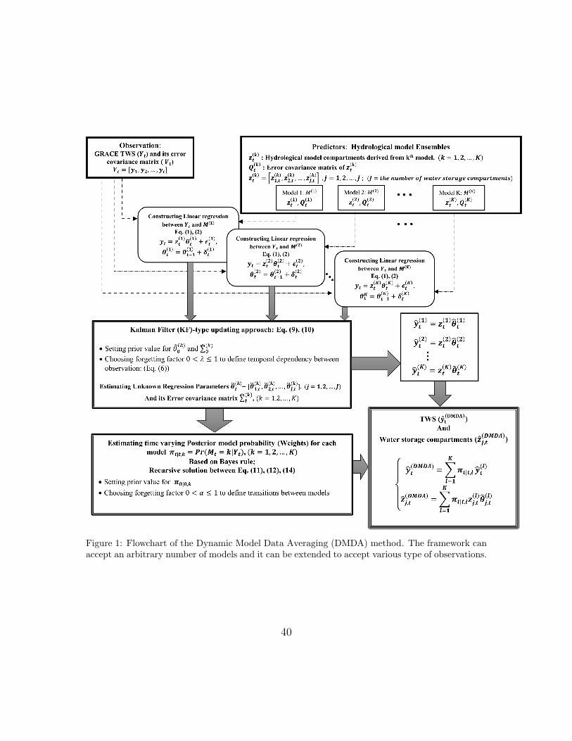
Figure 1: Flowchart of the Dynamic Model Data Averaging (DMDA) method. The framework canaccept an arbitrary number of models and it can be extended to accept various type of observations.
40

Figure 2: A synthetic example, where DMDA is applied in a controlled set up, to integrate 2hydrological models (here selected as SURFEX-TRIP and LISFLOOD) with simulated observedTWS to separate its compartments (i.e., groundwater and soil moisture). All data sets in thissimulation is related to the Niger River Basin and covering the period between 2002–2012; Figure2 (A) shows TWS simulated from PCR-GLOBWB (here standing in for observed TWS); Figure2 (B) shows the time series of groundwater and soil moisture derived from model 1 (B1, B3) andmodel 2 (B2, B4), which are considered as the input predictors in DMDA; Figure 2 (C1) presents thetime varying weights estimated for two selected model,and Figure 2 (C2) shows the reconstructed ofweights in the second step of our simulation. Figure 2 (D1) and (D2) show the updated hydrologicalcomponents obtained from the DMDA and BMA method and comparison between the obtainedresults and the expected values derived form simulated observation data.
41

Figure 3: Posterior model probabilities for the six initially considered models, over 10 selected riverbasins with the biggest RMSEs computed using GRACE and models-derived TWS. In the middleof Fig 3 the most contributed models in the DMDA-derived TWS are shown over the world’s 33largest river basins, covering the period of 2002–2012.
42

Figure 4: Long-term (2002–2012) linear trend in the DMDA-derived groundwater (a1), soil moisture(b1), and surface water (c1) components, expressed in mm/yr. The uncertainty of these fitted lineartrends are shown in (a2), (b2), (c2) respectively.
43

Figure 5: Correlation coefficients and their lags between the ENSO (-Nino 3.4 index) and ground-water estimates derived from the DMDA method and hydrological models used in this study forthe period of 2002–2012.
44

Figure 6: Correlation coefficients and their lags between the ENSO (-Nino 3.4 index) and soilmoisture estimates derived from the DMDA method and hydrological models used in this study forthe period of 2002–2012.
45

Figure 7: Correlation coefficients and their lags between the ENSO (-Nino 3.4 index) and surfacewater estimates derived from the DMDA method and hydrological models used in this study forthe period of 2002–2012.
46

Table 1: Overview of models used in this study and their water storage components.
Water Storage CompartmentsModel GroundWater Soil layer Surface
WaterCanopy Snow Snow
layerWater Use
PCR-GLOBWB Yes 2 Yes Yes Yes 1 NoW3RA Yes 3 No No Yes 1 No
HBV-SIMREG Yes 1 No No Yes 1 NoSURFEX-TRIP Yes 14 Yes Yes Yes 12 NoLISFLOOD Yes 2 No No Yes 1 YesORCHIDEE No 11 Yes No Yes 6 irrigation
47

Table 2: An overview of satellite altimetry observation used to validate DMDA results.
Lake River BasinLake Latitude Satellite
Cyclemid range passpoint of pass
Nasser Nile23.31◦N
[22.91◦N 23.66◦N] 94 4832.83◦E
Tana Nile12.11◦N
[11.95◦N 12.19◦N] 94 3837.40◦E
chad Niger13.01◦N
[12.94◦N 13.05◦N] 248 2514.38◦E
Kainiji Niger10.49◦N
[10.40◦N 10.50◦N] 135 214.50◦E
Malawi Zambezi10.84◦S
[12.042◦S 9.70◦S] 44 434.40◦E
Tanganyika Zambezi6.41◦S
[8.44◦S 4.461◦S] 222 1129.23◦E
Guri Orinoco7.37◦N
[7.06◦N 7.67◦N 152 69117.12◦W
Winnipeg Nelson53.18◦N
[52.82◦N 53.55◦N] 195 998.21◦W
Winnipegosis Nelson51.91◦N
[51.85◦N 52.05◦N 195 17100.01◦W
Erie St. Lawrence42.11◦N
[41.60◦N 42.54◦N] 193 4581.48◦W
Ontario St. Lawrence43.56◦N
[43.35◦N 43.83◦N] 15 3677.47◦W
Tharthar Euphrates33.87◦N
[33.75◦N 34.00◦N] 133 7043.37◦E
Urmia Euphrates37.25◦N
[37.25◦N 37.31◦N] 133 445.45◦E
Chany Ob54.96◦N
[54.94◦N 55.02◦N] 5 2877.33◦E
48

Table 3: Magnitude of simulated predictors, observations, and DMDA results in a controlled syn-thetic simulation.
Hydrological Compartment Model nameMin Max RMS[mm] [mm] [mm]
Groundwater (First model) LISFLOOD -10.5 16.1 7.9Groundwater (Second model) SURFEX-TRIP -12.1 39.8 14.2Groundwater (Expected value of DMDA) PCR-GLOBWB -39.5 70.4 24.2Groundwater (DMDA result) DMDA Output -35.3 92.3 19.9Groundwater (BMA result) BMA Output -46.0 130.2 43.8
Soil Moisture (First model) LISFLOOD -37.4 62.2 30.8Soil Moisture (Second model) SURFEX-TRIP -45.7 79.9 41.5Soil Moisture (Expected value of DMDA) PCR-GLOBWB -52.0 107.9 48.7Soil Moisture (DMDA result) DMDA Output -58.5 113.8 51.2Soil Moisture (BMA result) BMA Output -40.8 49.6 21.0
TWS (First model) LISFLOOD -46.8 75.5 37.2TWS (Second model) SURFEX-TRIP -57.6 115.2 54.6TWS (Expected value of DMDA results) PCR-GLOBWB -83.3 164.5 64.2TWS (DMDA result) DMDA Output -77.8 153.8 63.2TWS (BMA result) BMA Output -77.8 153.8 63.2
|∆|Groundwater |LISFLOOD− Expected value| 0 58.1 11.2|∆|Groundwater |SURFEX− Expected value| 0 45.8 10.3|∆|Groundwater |DMDA− Expected value| 0 31.2 5.3|∆|Groundwater |BMA− Expected value| 0 87.6 20.4
|∆|Soil Moisture |LISFLOOD− Expected value| 0 46.8 9.6|∆|Soil Moisture |SURFEX− Expected value| 0 29.3 5.7|∆|Soil Moisture |DMDA− Expected value| 0 29.2 5.2|∆|Soil Moisture |BMA− Expected value| 0 89.5 18.6
|∆|TWS |LISFLOOD− Expected value| 0 94.7 18.6|∆|TWS |SURFEX− Expected value| 0 60.9 14.1|∆|TWS |DMDA− Expected value| 0 24.2 6.2|∆|TWS |BMA− Expected value| 0 31.4 8.4
49

Table 4: The amplitude of linear trend [mm/yr] and its uncertainty, fitted to the DMDA-derivedgroundwater, soil Moisture, and surface water, during 2002–2012.
Basin DMDA DMDA DMDA
ID Name GroundWater Soil Moisture Surface Water
1 Amazon 0.17 ± 0.12 -1.92 ± 0.09 1.43 ± 0.062 Amur 0.46 ± 0.06 2.61 ± 0.09 0.25 ± 0.033 Aral 0.02 ± 0.08 -1.43 ± 0.22 0.21 ± 0.124 Brahmaputra -0.44 ± 0.16 -7.00 ± 0.69 -0.13 ± 0.215 Caspian-Volga -2.06 ± 0.15 -2.98 ± 0.16 -0.02 ± 0.076 Colorado 0.80 ± 0.11 -0.75 ± 0.09 0.82 ± 0.087 Congo -0.72 ± 0.08 0.59 ± 0.03 0.06 ± 0.068 Danube -0.47 ± 0.18 -0.75 ± 0.21 -0.08 ± 0.049 Dnieper -0.5 ± 0.29 -2.27 ± 0.28 -0.03 ± 0.1810 Euphrates -5.36 ± 0.23 -5.75 ± 0.39 -2.09 ± 0.0911 Lake Eyre 0.55 ± 0.16 2.42 ± 0.19 0.77 ± 0.0412 Ganges -14.77 ± 0.25 2.69 ± 0.40 0.29 ± 0.0513 Indus -8.26 ± 0.16 1.10 ± 0.13 -0.06 ± 0.0714 Lena 1.74 ± 0.11 1.94 ± 0.05 0.20 ± 0.0815 Mackenzie 0.51 ± 0.06 0.12 ± 0.05 -0.05 ± 0.1016 Mekong 1.58 ± 0.43 -0.79 ± 0.33 0.83 ± 0.1717 Mississippi 1.25 ± 0.09 1.36 ± 0.09 0.33 ± 0.0218 Murray 0.06 ± 0.06 6.66 ± 0.15 -1.47 ± 0.0419 Nelson 0.70 ± 0.18 2.45 ± 0.15 0.11 ± 0.0320 Niger -1.14 ± 0.15 0.75 ± 0.15 0.32 ± 0.0521 Nile 0.45 ± 0.06 0.77 ± 0.06 -0.05 ± 0.0222 Ob -1.42 ± 0.08 -1.54 ± 0.06 0.05 ± 0.0723 Okavango 1.74 ± 1.31 3.92 ± 0.55 -1.42 ± 0.3724 Orange 1.32 ± 0.05 1.28 ± 0.06 -0.85 ± 0.0525 Orinoco 0.87 ± 0.11 3.45 ± 0.26 -0.22 ± 0.1926 Parana 0.68 ± 0.08 0.03 ± 0.13 1.04 ± 0.0427 St. Lawrence 1.49 ± 0.18 1.07 ± 0.07 0.48 ± 0.0528 Tocantins 2.41 ± 0.47 2.37 ± 0.35 0.08 ± 0.2129 Yangtze 0.55 ± 0.23 -0.30 ± 0.09 0.20 ± 0.0230 Yellow -3.50 ± 0.14 -0.27 ± 0.05 0.08 ± 0.2131 Yenisei -0.26 ± 0.07 1.79 ± 0.06 0.75 ± 0.1132 Yukon -4.73 ± 1.08 -1.52 ± 0.20 -1.11 ± 0.2333 Zambezi 1.19 ± 0.38 0.65 ± 0.31 0.35 ± 0.25
50

Table 5: Correlation between satellite altimetery observation and: I) TWS , II) Surface Water(SW) derived from GRACE, DMDA, and individual models, during 2002–2012.
Correlation between Altimetry Obs. and:
Basin
Waterstorage
GRACE
DMDA
PCR-G
LOBW
B
SURFEX-T
RIP
LISFLOOD
HBV-SIM
REG
W3RA
ORCHID
EE
Nile TWS 0.358 0.381 0.326 0.239 0.095 -0.082 0.001 0.180
(Nasser Lake) SW - 0.462 0.363 0.441 - - - -0.046
Nile TWS 0.682 0.718 0.602 0.569 0.517 0.302 0.231 0.635
(Tana Lake) SW - 0.492 0.340 0.603 - - - 0.455
St. Lawrence TWS 0.353 0.261 0.271 0.010 -0.121 -0.114 -0.087 -0.010
(Erie Lake) SW - 0.432 0.483 0.126 - - - 0.227
St. Lawrence TWS 0.410 0.364 0.353 0.110 -0.063 -0.064 -0.023 0.037
(Ontario Lake) SW - 0.582 0.572 0.273 - - - 0.239
Euphrates TWS 0.698 0.569 0.225 0.021 0.103 -0.057 0.043 0.182
(Tharthar Lake) SW - 0.236 0.127 0.093 - - - -0.282
Euphrates TWS 0.737 0.628 0.223 0.080 0.148 0.021 0.095 0.185
(Urmia Lake) SW - 0.172 0.170 0.131 - - - -0.325
Ob TWS 0.393 0.482 0.371 0.303 0.336 0.338 0.348 0.328
(Chany Lake) SW - 0.296 0.278 0.177 - - - -0.333
Zambezi TWS 0.552 0.632 0.362 0.277 0.346 0.225 0.246 0.391
(Malawi Lake) SW - 0.382 0.247 0.410 - - - 0.394
Zambezi TWS 0.414 0.365 0.231 0.192 0.121 0.117 0.128 0.160
(Tanganyika Lake) SW - 0.243 0.096 0.241 - - - -0.093
Niger TWS 0.576 0.558 0.436 0.318 0.308 0.065 0.188 0.519
(Chad Lake) SW - 0.657 0.511 0.616 - - - 0.689
Niger TWS 0.132 0.102 -0.002 -0.149 -0.174 -0.383 -0.278 0.079
(Kainiji Lake) SW - 0.282 0.126 0.200 - - - 0.214
Orinoco TWS 0.585 0.539 0.332 0.427 0.431 0.321 0.301 0.434
(Guri Lake) SW - 0.421 0.314 0.390 - - - 0.318
Nelson TWS 0.285 0.270 0.139 -0.185 -0.444 -0.440 -0.389 -0.279
(Winnipeg Lake) SW - 0.104 -0.290 0.072 - - - 0.012
Nelson TWS 0.216 0.249 0.238 0.135 -0.09 -0.164 -0.088 -0.065
(Winnipegosis Lake) SW - 0.098 -0.321 -0.015 - - - -0.480
51