Comparing different searches

for gravitational-wave bursts on simulated LIGO and VIRGO data

Michele Zanolin -MITon behalf of the LIGO-VIRGO joint working group

• Benefits

• Pipeline

• Results

• Future plans

Benefits of comparing LIGO and Virgo searches

on single interferometer simulated data • Compare time domain and frequency domain methods over

different class of waveforms.

• Detector independent measure of performance

• Simulated noise (see inspiral talk) allows to test the limit of design sensitivity and improved vetos (and no restrictions due to use of real data)

• Single interferometer analysis decouples the properties of the trigger generation from those of coincidence modules

• Events might happen when only one interferometer is on lock

Pipeline• 7 methods already involved (3 more will join soon) • Simulated data have been produced• Simulated injections have been generated • Receiver operating characteristics have been computed on the 3

hours of simulated data for false rates from 0.1 to 0.0001 Hz.• Trigger lists ( containing rough time-frequency volume) and sets

of figures of merit have been generated• A method independent parameterisation of the triggers is adopted

(Sylvestre, Sutton, Lazzarini). A post processing stand alone parameter estimation module is introduced, that uses Maximum likelihood estimators and assumes colored Gaussian noise (Zanolin, Sylvestre).

Time-frequency Methods • Q-pipeline (see talk by S.Chatterji): multiresolution time frequency

search for excess power applied on data that are first whitened using zero phase linear prediction. Equivalent to optimal matched filter for minimum uncertainty waveforms of unknown phase in the whitened data.

• Kleine Welle (L.D. - L. Blackburn): search for statistically significant clusters of coefficients in the dyadic Haar wavelet decomposition.

• S-transform (V.D. - see talk byA.C. Clapson): search for statistically significant clusters of coefficients in the time frequency map generated using a kernel composed of complex exponentials shaped by Gaussian profiles with width inversely proportional to frequency. High pass and line removal applied on Virgo data.

• Power Filter (G.Guidi): search for excess power over different time intervals and sets of frequencies.

Time domain methods

• Peak Correlator (P.Hello): Search for peaks of Wiener filtered data with Gaussian templates. For Virgo data a high pass filter and a line removal filter are applied to remove the resonance at 0.6 Hz.

• Mean Filter (M. A. Bizouard): Search for excess in moving averages of whitened data over intervals containing from 10 to 200 samples.

• ALF (M.A.Bizouard): Search for change in slope over moving windows of whitened data over intervals containing from 10 to 300 samples.

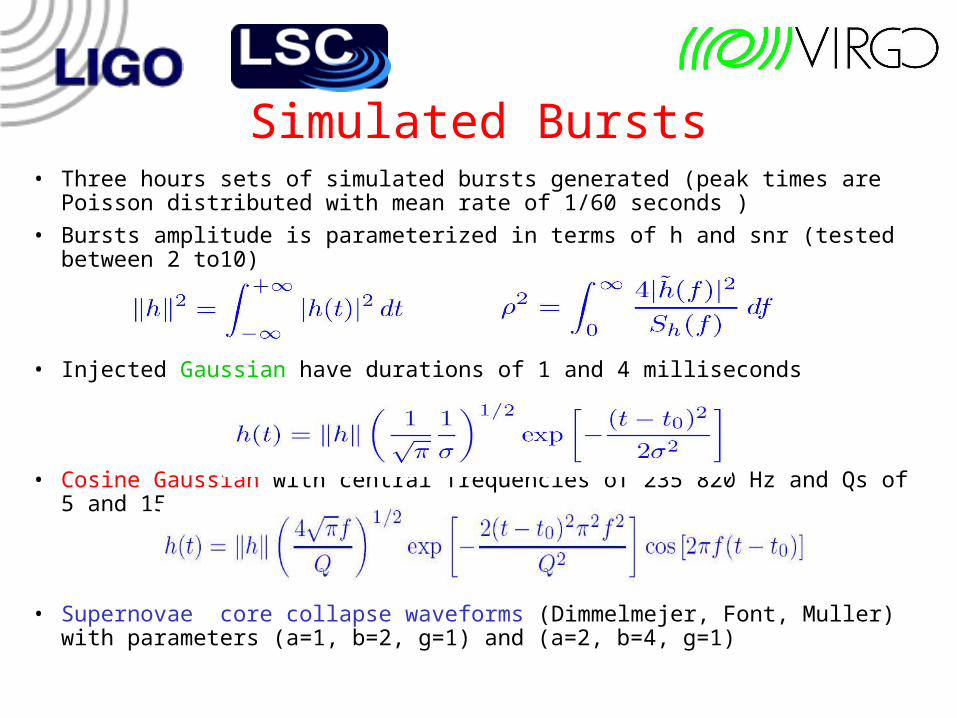
Simulated Bursts• Three hours sets of simulated bursts generated (peak times are Poisson

distributed with mean rate of 1/60 seconds )

• Bursts amplitude is parameterized in terms of h and snr (tested between 2 to10)

• Injected Gaussian have durations of 1 and 4 milliseconds

• Cosine Gaussian with central frequencies of 235 820 Hz and Qs of 5 and 15

• Supernovae core collapse waveforms (Dimmelmejer, Font, Muller) with parameters (a=1, b=2, g=1) and (a=2, b=4, g=1)

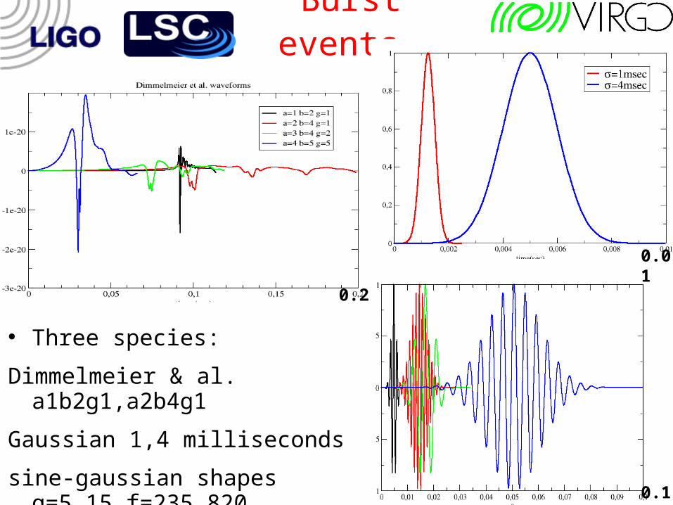
Burst events

● Three species:

Dimmelmeier & al. a1b2g1,a2b4g1

Gaussian 1,4 milliseconds

sine-gaussian shapes q=5,15 f=235,820

0.2

0.1

0.01

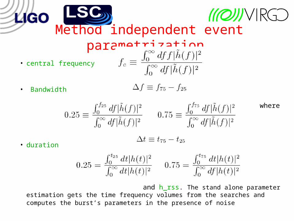
Method independent event parametrization

• central frequency

• Bandwidth where

• duration where

and h_rss. The stand alone parameter estimation gets the time frequency volumes from the searches and computes the burst’s parameters in the presence of noise

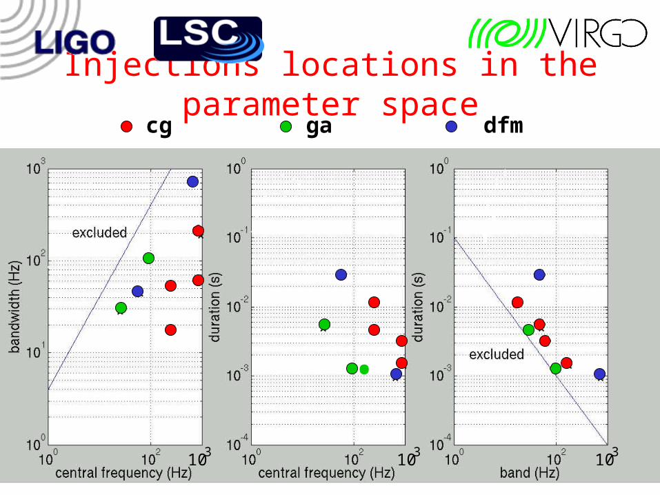
Injections locations in the parameter space

..

10 10103 33

cg ga dfm

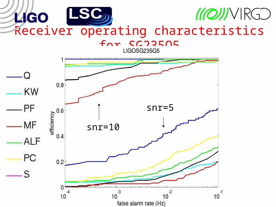
Receiver operating characteristics for SG235Q5

snr=10

snr=5

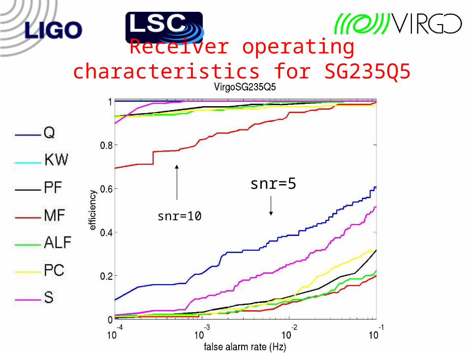
Receiver operating characteristics for SG235Q5

snr=5

snr=10

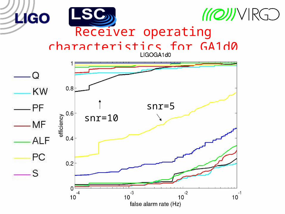
Receiver operating characteristics for GA1d0

snr=10snr=5

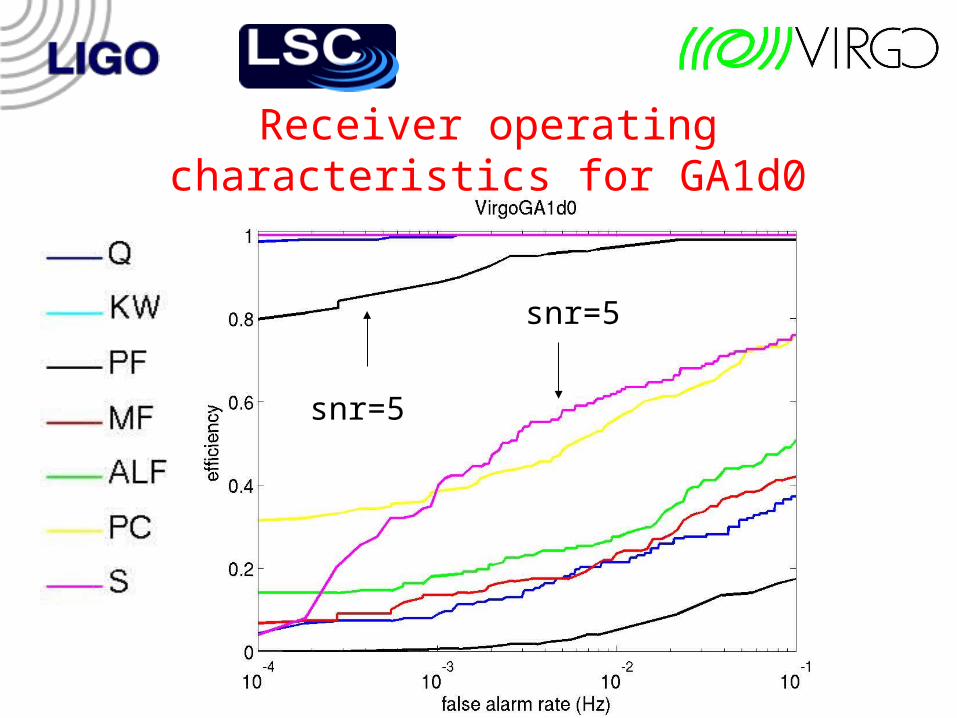
Receiver operating characteristics for GA1d0

snr=5

snr=5

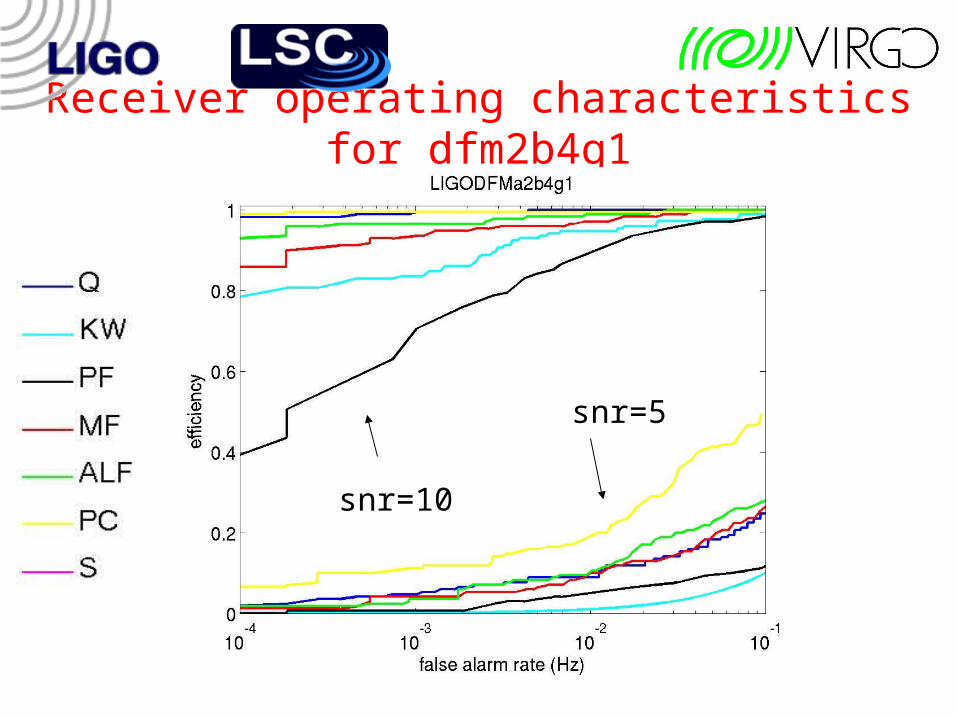
Receiver operating characteristics for dfm2b4g1

snr=10

snr=5

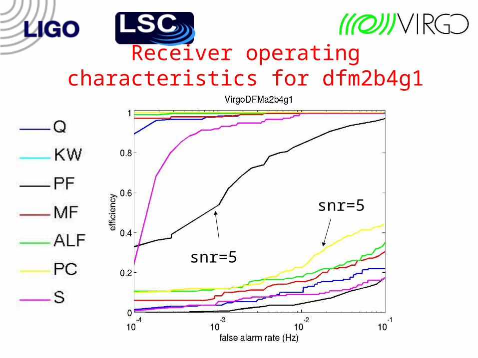
Receiver operating characteristics for dfm2b4g1

snr=5

snr=5

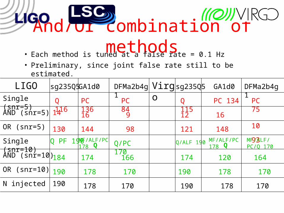
And/Or combination of methods

lLIGOSingle (snr=5)

AND (snr=5)

OR (snr=5)

AND (snr=10)

OR (snr=10)

Single (snr=10)

N injected

sg235Q5 sg235Q5

14

130

Q PF 190

184

190

178

144

DFMa2b4g1Virgo

Q 116

16 9

PC 84PC 136

93

DFMa2b4g1GA1d0 GA1d0

16

121

PC 75PC 134

12

Q 115

10

98 148

Q/PC 170MF/ALF/PC 178

164174

Q/ALF 190

178 170

174 166

190 178 170

190 190170 170178

MF/ALF/PC 178

MF/ALF/PC/Q 170

120

• Each method is tuned at a false rate = 0.1 Hz

• Preliminary, since joint false rate still to be estimated.

Q Q

What did we learn

• Learn to process each others' data, exchange, and compare triggers

• Different methods perform differently in different regions of the parameter space

• OR combinations of methods increases efficiency (false rates for combinations of the methods still to be investigated)

• Confront burst search performance with optimal matched filtering (see S.Chatterji talk)

Future directions• As first project of exchanging simulated noise and signal data of the

LIGO and Virgo instruments is successfully carrying out and address the goals set by the joint working group the next steps are approaching:

- A program to continue the data exchange within the framework of simulated data but using astrophysical (coherent) waveform injections onto simulations is forthcoming (useful to quantify the scientific potential of a combined analysis )

- Ultimate goal is to operate the instruments as part of a global network.

We are defining the details of exchange of triggers (and/or) data will

actually take place.

From now on back up material

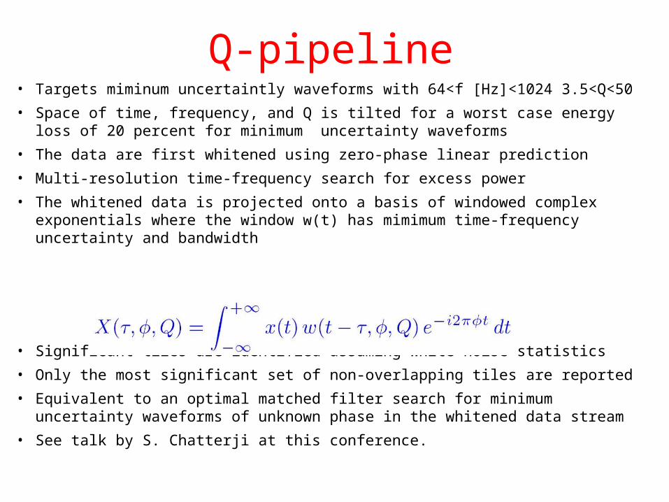
Q-pipeline• Targets miminum uncertaintly waveforms with 64<f [Hz]<1024 3.5<Q<50

• Space of time, frequency, and Q is tilted for a worst case energy loss of 20 percent for minimum uncertainty waveforms

• The data are first whitened using zero-phase linear prediction

• Multi-resolution time-frequency search for excess power

• The whitened data is projected onto a basis of windowed complex exponentials where the window w(t) has mimimum time-frequency uncertainty and bandwidth

• Significant tiles are identified assuming white noise statistics

• Only the most significant set of non-overlapping tiles are reported

• Equivalent to an optimal matched filter search for minimum uncertainty waveforms of unknown phase in the whitened data stream

• See talk by S. Chatterji at this conference.

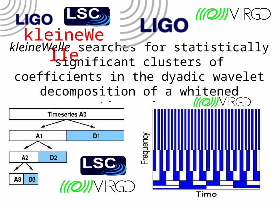
kleineWellekleineWelle searches for statistically significant

clusters of coefficients in the dyadic wavelet decomposition of a whitened timeseries.

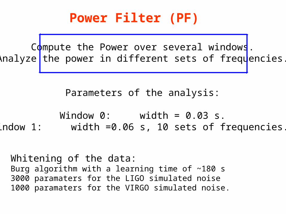
Power Filter (PF)

Compute the Power over several windows.Analyze the power in different sets of frequencies.

Parameters of the analysis:

Window 0: width = 0.03 s.Window 1: width =0.06 s, 10 sets of frequencies.

Whitening of the data: Burg algorithm with a learning time of ~180 s3000 paramaters for the LIGO simulated noise1000 paramaters for the VIRGO simulated noise.

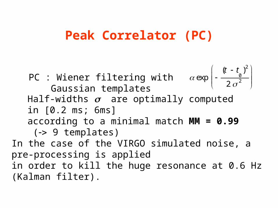
Peak Correlator (PC)

2

2

0

2

)(exp

ttPC : Wiener filtering with Gaussian

templatesHalf-widths are optimally computed in [0.2 ms; 6ms] according to a minimal match MM = 0.99 ( 9 templates)

In the case of the VIRGO simulated noise, a pre-processing is appliedin order to kill the huge resonance at 0.6 Hz (Kalman filter).

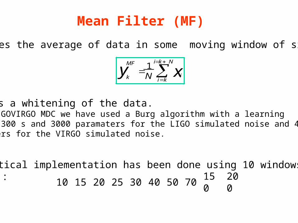
Mean Filter (MF)

Nki

kii

MF

k xy N1

MF computes the average of data in some moving window of size N :

MF needs a whitening of the data. In the LIGOVIRGO MDC we have used a Burg algorithm with a learning time of 300 s and 3000 paramaters for the LIGO simulated noise and 4000 paramaters for the VIRGO simulated noise.

The practical implementation has been done using 10 windows : N (bins) : 20

0150 70 50 40 30 25 20 15 10

ALF

taxb22

ttxttxa

)1(2

ba

ba

yk

)12(

20

122

NN

f

a )1(242

NNN

b )12

1(

23

NN

yyykk

ALF

k

22

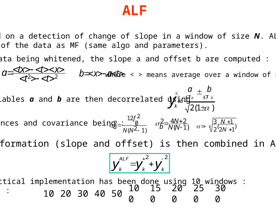
ALF is based on a detection of change of slope in a window of size N. ALF needsa whitening of the data as MF (same algo and parameters).

Assuming data being whitened, the slope a and offset b are computed :

where < > means average over a window of size N

The variables a and b are then decorrelated using

variances and covariance being :

All the information (slope and offset) is then combined in ALF :

300

250 200 150 100 50 40 30 20 10

The practical implementation has been done using 10 windows : N (bins) :

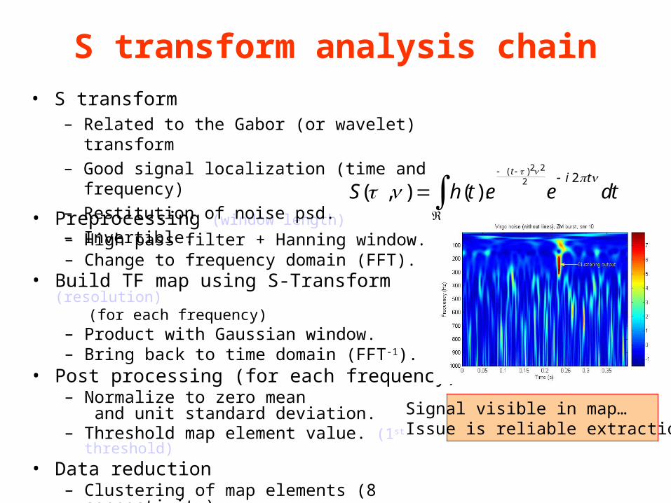
• Preprocessing (window length)– High pass filter + Hanning window.– Change to frequency domain (FFT).

• Build TF map using S-Transform (resolution) (for each frequency)

– Product with Gaussian window.– Bring back to time domain (FFT-1).

• Post processing (for each frequency)– Normalize to zero mean

and unit standard deviation.– Threshold map element value. (1st threshold)

• Data reduction– Clustering of map elements (8 connectivity)– Threshold on total cluster energy. (2nd threshold)

• S transform– Related to the Gabor (or wavelet) transform

– Good signal localization (time and frequency)

– Restitution of noise psd.

– Invertible.

dteethSti

t

22

22)(

).(),(

S transform analysis chain

Signal visible in map…Issue is reliable extraction!