Comparing and forecasting performances indifferent events of athletics using a

probabilistic model

Brian GodseySchool of Medicine,

University of Maryland,Baltimore, MD, USA

brian@briangodsey.com

Published in the Journal of Quantitative Analysis in Sports inJune 2012

AbstractThough athletics statistics are abundant, it is a difficult task to quantitatively com-pare performances from different events of track, field, and road running in ameaningful way. There are several commonly-used methods, but each has itslimitations. Some methods, for example, are valid only for running events, orare unable to compare men’s performances to women’s, while others are basedlargely on world records and are thus unsuitable for comparing world records toone other. The most versatile and widely-used statistic is a set of scoring tablescompiled by the IAAF, which are updated and published every few years. Un-fortunately, these methods are not fully disclosed. In this paper, we propose astraight-forward, objective, model-based algorithm for assigning scores to ath-letic performances for the express purpose of comparing marks between differentevents. Specifically, the main score we propose is based on the expected numberof athletes who perform better than a given mark within a calendar year. Comput-ing this naturally interpretable statistic requires only a list of the top performancesin each event and is not overly dependent on a small number of marks, such asthe world records. We found that this statistic could predict the quality of fu-ture performances better than the IAAF scoring tables, and is thus better suitedfor comparing performances from different events. In addition, the probabilistic

1

arX

iv:1

408.

5924

v1 [

stat

.AP]

25

Aug

201

4

model used to generate the performance scores allows for multiple interpretationswhich can be adapted for various purposes, such as calculating the expected topmark in a given event or calculating the probability of a world record being brokenwithin a certain time period. In this paper, we give the details of the model andthe scores, a comparison with the IAAF scoring tables, and a demonstration ofhow we can calculate expectations of what might happen in the coming Olympicyear. Our conclusion is that a probabilistic model such as the one presented hereis a more informative and more versatile choice than the standard methods forcomparing athletic performances.

1 IntroductionQuantitatively comparing performances from different athletic events and speci-fying how much more impressive one performance is than another are not sim-ple tasks. There are a few good models that are valid for running events, par-ticularly longer distances, namely those by McMillan (2011), Cameron (1998),Riegel (1977), and Daniels and Gilbert (1979). These models rely on physiologi-cal measurements such as speed and running economy to compare performancesat different race distances, either for men or for women, but not between them.

Purdy Points (Gardner and Purdy, 1970) have long been used to comparemarks from different events in both track and field, but these scores are basedmainly on the world records of each event at a particular date in the past, whichleads to two main disadvantages: (1) it is impossible to compare world recordsto each other if the model is based on them, and (2) basing the model on such asmall data set leads to much uncertainty and variation in the scores as the recordsand model evolve over time. In other words, if a particular world record is “weak”in some sense, Purdy points will likely unfairly assign a higher score to perfor-mances in that event when compared to others.

Currently, the most popular method for comparing performances across allevents in track and field as well as road running is to consult the IAAF scoringtables (Spiriev and Spiriev, 2011). These tables are updated every few years usingmethods that are not fully disclosed, with the last two updates occurring in 2008and 2011. The IAAF is the main official governing body for international athlet-ics, and they also publish the official scoring tables for “combined events compe-titions” such as the heptathlon and decathlon. These “combined events” consistof seven women’s and ten men’s events, respectively, and which are contested atmost major international athletics competitions, and the winner is declared to bethe competitor with the highest point total from all of the events. These combinedevents scoring tables were intended to assign a similar amount of points to a per-formances that are “similar in quality and difficulty” (International Association of

2

Athletics Federations, 2001). All point values P in these tables can be calculatedusing a formula of the form P = a(M−b)c, where M is the measured performance(use M =−T for running times T , where a lower performance is better) and a, b,and c are constants estimated by undisclosed methods (International Associationof Athletics Federations, 2001). The combined events tables are not the same asthe general IAAF scoring tables, but it may be deduced that both sets of tablesare produced using similar methods. Which data are used and how exactly theconstants are estimated is not clear.

In this publication, we introduce a method of scoring athletic performancesbased on the idea that a good performance is a rare or improbable performance.Two very common reasons why one might think that an athletic performance isgood are:

1. A performance is good if few athletes improve upon it, or

2. A performance is good if it is close to or improves upon the [previous] bestperformance.

The first reason is important because it puts emphasis on what has actuallyhappened. In other words, if an athlete is in the top ten in the world in her event,she is likely better than an athlete who is ranked 50th or 100th. On the otherhand, the second reason is important because it focuses more on what is possible.Sometimes in sport, a revolution occurs, whether in training, technique, equip-ment, or facilities, and performances improve dramatically. Certain events in his-tory cause people to re-think what they thought was good—Bob Beamon’s 1968Olympic long jump in Mexico City, Paula Radcliffe’s 2003 London Marathon, andmore recently Usain Bolt’s 2009 World Championship 100m run in Berlin cometo mind. In some of these cases, but not in others, what we once thought wasunthinkable becomes commonplace. In 1996, many people thought that MichaelJohnson’s 200m world record would last an eternity—it was revolutionary—butnow it is only fourth on the all-time list. The men’s marathon record has droppedtremendously in recent years, carried in part by Haile Gebreselassie and Paul Ter-gat, who accomplished the same feat for the 10,000m run in the 1990s. Thepoint is only that a superb, dominating performance might be one of the great-est feats ever witnessed, but it also might be an inevitability. Usain Bolt’s 9.58smark in the Berlin 100m dash in 2009 is certainly impressive, but we saw threemen running 9.72s or faster in the 100m dash in 2008, all under the world recordfrom 2007; so how impressive was 9.58s really? Is it a statistical outlier, or is it theexpected result of a general increase in performance level which by chance hadnot yet produced the outstanding performance that was bound to happen? Theseare some questions this paper was intended to answer.

3

The methods introduced here utilize a large amount of historical data to esti-mate directly the improbability of athletic performances. Using a data set consist-ing of the top n performances of all time—where n is generally well over 100 andcan be different for each event—we estimate a log-normal distribution for eachevent, allowing us to calculate directly both the probability that a specific markis exceeded as well as the expected number of such performances within a giventime period. We use this model to predict the number and quality of top perfor-mances in the subsequent years, for data up until the year 2000 and also 2008, andwe show that our scoring tables based on data prior to 2008 correlate more highlywith actual data than do the 2008 IAAF scoring tables. Lastly, we look aheadto the coming year and the 2012 Olympic Games in London, and we determinewhich world records are most in danger of being broken and which are most likelyto last a while longer.

2 MethodsIn general, we estimate a log-normal distribution for each athletic event k using alist of the best nk marks from that event. Equivalently, we assume that the naturallogarithms of performances from each event are normally distributed. We use thissecond formulation throughout this paper.

A list of best marks represents only one tail of the distribution, and so forsimplicity we convert marks so that we perform all calculations on the lower tail.For running events, a lower time is better, and thus we take only the natural log-arithm of the times, in seconds, before fitting a normal distribution to the data.For throwing and jumping events, a higher mark is better, so we assume that theinverse (negative) of the natural logarithm is normally distributed. This does notcause any adverse consequences as long as we again take the inverse before con-verting back to an actual mark, typically in centimeters (cm).

Figure 1 illustrates how a normal distribution can be fit to a list of top [log-]performances, represented by a histogram. Since we are working exclusivelywith the tail of the distribution, the parameters must be estimated from the shapeof the tail.

In our first set of analyses, we fit the model to the data as it would have beenat the beginning of 2000, and we test its predictive ability for the subsequentyears. Below, we elaborate on exactly how we calculate these predictions andtheir comparison with actual outcomes.

In the second set of analyses, we fit the model to the data as it would have beenat the beginning of 2008, and we test its predictive ability for the following fouryears. Then we generate a set of scoring tables analogous to the IAAF scoringtables and we compare some predictions that could be made from the tables to

4

mens400m

log(performance)

Tota

l num

ber

of p

erfo

rman

ces

3.78 3.80 3.82 3.84 3.86

010

020

030

0

mens400m

log(performance)

Tota

l num

ber

of p

erfo

rman

ces

3.77 3.78 3.79 3.80 3.81

050

100

200

Figure 1: Illustration of model fit. Both panels in this figure show a histogramof log-performances for the men’s 400m dash (all data until the present day) aswell as the fitted normal distribution curve that is re-scaled to match the histogram.The left panel gives a wider view, while the right panel shows in more detail thearea of the graph which contains performances appearing on the list of top marks.

those of the IAAF scoring tables. Granted, the IAAF may not have intended forsuch specific predictions to be made, but we try to be as fair as possible basedon what it might mean for one athletic performance to be “better” than another.We think that, generally, performances that are given equal scores should, in anygiven year, (1) have approximately the same number of marks exceed them, (2)should have the same chance of being broken, and (3) should have a comparablerelative margin (in percent) between itself and the best mark of the year.

We then give the results of a third set of analyses that uses data through Oc-tober 1st, 2011, including predictions about the numbers of top performances thatwill occur in the coming years as well as what we expect the top mark to be ineach event and the probabilities of new world records being set.

2.1 DataAn ideal data set would consist of a complete list of every performance by anelite athlete in the modern era of athletics. Such a list, as far as we can tell, doesnot exist. We do have, however, lists of the best performances ever. The listscompiled by www.alltime-athletics.com (Larsson, 2011) include all of thetop performances of all time—list lengths ranging from a few hundred to severalthousand, depending on the event. We have data for all track and field events con-tested in the modern Olympic Games for men and women, except the heptathlonand decathlon, plus the marathon, half marathon, one mile run and 3000m run.

5

We assume that these lists are complete, in the sense that each list is indeed thebest nk performances for event k, with no missing marks.

For the three time periods we consider—to which we will refer by year, 2000,2008, and 2012—we do two sets of analyses, one using all data prior to that year,and the other using data from only the prior 5 years.

The performance lists for performances prior to the present day (1 Octo-ber 2011) have lengths between 215 and 9672, with a median of 1596.5. Forthe five years prior to the present day, list lengths range from 10 to 4630, witha median of 275. The women’s one mile run is the shortest list, and the secondshortest list has 51 entries.

The performance lists for performances prior to 2008 have lengths between205 and 5547, with a median of 1273. Using five years of data prior to 2008gives a range of list lengths from 18 to 4235, with a median of 298.5. The listof length 18 belongs to the women’s one mile run, and the next shortest is thewomen’s shot put, with 38 entries. These are special cases where either the eventis rarely contested (one mile run) or has a dearth of recent top performances (shotput). All other lists include at least 68 performances.

The performance lists for performances prior to 2000 have lengths between63 and 3761, with a median of 790. For the five years prior to 2000, list lengthsrange from 52 to 1288, with a median of 252.5.

2.2 The modelA normal (or log-normal) distribution takes two parameters: mean µ and vari-ance σ2. Given these parameters, we can calculate the probability pa that a par-ticular performance in event k exceeds a specified mark a using the formula:

pa =

a∫−∞

N(x | µk,σ2k )dx (1)

where a is a specified performance (natural logarithm of a mark, inverted forevents in which greater marks are better) and N(x | µk,σ

2k ) is the normal dis-

tribution probability density function (pdf). Equation 1 is equivalent to the cu-mulative distribution function (cdf) of the normal distribution with mean µk andvariance σ2

k , which we call F(a | µk,σ2k ). If we accurately estimate µk and σ2

k ,then pa is easy to compute.

We can use F(a | µk,σ2k ) to formulate the pdf of a normal distribution trun-

cated at ck as:

6

pk(x | µk,σ2k ) =

N(x|µk,σ

2k )

F(ck|µk,σ2k )

for x≤ ck

0 elsewhere(2)

Bayes’ Theorem then gives the un-normalized posterior density for the modelparameters:

`(µk,σ2k | Xk) = ∏

x∈Xk

N(x | µk,σ2k )p(µk)p(σ2

k )

F(ck | µk,σ2k )

(3)

where Xk is the set of performances on the list for event k, and p(µk) and p(σ2k )

are the prior probability distributions of µk and σ2k , respectively.

2.3 Development of an empirical priorIn general, we would like to use non-informative prior distributions for our modelparameters µk and σ2

k , but when first fitting our model to the data, it quicklybecame clear that there was much uncertainty about the total population size Nkfor each event k. So, we used an empirical Bayes approach to estimate reasonableprior expectations for the Nk in order to reduce this uncertainty.

That is, the posterior densities suggested that when using non- or weakly-informative priors for each event, many {µk,σ

2k } pairs were nearly equally likely,

and they gave a wide range of values for Nk, as calculated according to the follow-ing relation:

F(wk | µk,σ2k ) =

nk

Nk(4)

where, nk is the [constant] length of the list of best performances for event k,and wk is the worst mark on that list. Equation 4 is inherently true, as it saysonly that the cumulative density through the region for which we have data—i.e.the tail—is equal to the size of the data set, nk, divided by the size of the largestpossible data set, Nk.

In order to reduce this uncertainty over the Nk and ensure that the estimatedpopulation sizes for different events were similar, we re-parametrized the model,using equation 4, to use Nk as a parameter instead of σ2

k . Then, we assume a log-normal prior distribution for the Nk, with parameters µN and σ2

N , as well as a uni-form prior distribution over all real numbers for the µk, which is non-informativeand improper.

We would, ideally, optimize the parameters µN and σ2N of the prior for Nk, as

suggested by MacKay (1999), iteratively as we fit the model, but since the modelis fit independently for each event and because calculation takes a considerable

7

amount of time, we are not able to use many iterations. We chose to approxi-mate two such iterations, where in the first iteration we fit all models using a veryweakly-informative prior for Nk (i.e. µN = 10,000 and σ2

N = e20), and then, inthe second iteration, we re-fit the models with updated parameters µN and σ2

N ,which were optimized based on point estimates for the Nk. Specifically, we calcu-late from the first-iteration posterior distributions, for each k, the expected valueof Nk, E[Nk], and then using these estimates to update µN and σ2

N according to thefollowing:

µN = median({log(E[Nk]) : for all k}) (5)

σ2N = min

K⊂{all k}var({log(E[Nk]) : k ∈ K}) (6)

where the subset K comprises 75% of the set of all events. Thus, both priordistribution parameters µN and σ2

N are robust to some outlying Nk, which we en-countered in a few cases, particularly in events for which we have little data, aswell as with data from the sprints, high jump, and pole vault, because those dataare more discrete than others, as many competitors share the same mark. Wechose the value 75% somewhat arbitrarily, but it ensures that most of the data areused while allowing for inaccurate values due, for example, to small or highlydiscrete data sets. Updating the prior distribution for the Nk only once in thismanner gives a compromise between non-informative and fully optimized priors,while improving convergence and sharing some information between models fordifferent events.

While we do not expect the population sizes from different events to be identical—there are many reasons why there could be more participants or performances inone event than another—we do not expect them to be vastly different, either. Forexample, there are more marathon times posted each year than in any other event,though admittedly most are not elite times. Also, the one mile run and the 1500mrun are very similar in distance, yet each year there are far more 1500m races thanmile races. Sprinters tend to run more races each year than long distance runners,as well. On the other hand, we expect the population sizes to be relatively simi-lar, perhaps within an order of magnitude of each other, simply because—amongother reasons—awards, medals, and championships are generally identical in na-ture and quantity for most events, and identical incentive leads us to believe thatpopulation sizes would be approximately equal. We have tried to address this inchoosing our prior distributions.

2.4 Fitting the model to the dataTo fit the model (3) for each event, we use Markov chain Monte Carlo (MCMC)methods as implemented in the mcmc package (Geyer., 2010) of the R program-

8

ming language (R Development Core Team, 2008), which is a version of theMetropolis-Hastings algorithm (Hastings, 1970). We use a “burn in” period of 1,000steps, after which we test the sample acceptance rate, requiring it to be between 0.2and 0.4 (we found that this range generally gives good convergence), and if un-acceptable we re-do the burn-in with an adjusted sample step size. This processis automated. Following burn-in, we use a subsequent 1,000 batches of 50 stepseach with 10 random parameter initializations to determine the joint distributionof µk and σ2

k —and/or Nk—for each k.Convergence of the MCMC sampling was assessed visually using various

plots as well as using the multivariate diagnostic of Gelman and Rubin (1992)as implemented in the coda (Plummer, Best, Cowles, and Vines, 2006) packagein R (R Development Core Team, 2008).

2.5 Some meaningful statisticsThe value of pa as calculated in equation 1 can be interpreted as the probabilitythat in a given performance a specified member of the total elite athlete populationfor the given event performs better than the mark a. This is a natural measure ofperformance quality, but it is not easy to test its accuracy using real data. There-fore, in this section we give some other statistics based on the model that may bebetter at describing the performances we witness during an athletic season. Theyare based on the ideas stated in the introduction to this paper, that we can measurethe rarity—and quality—of a performance by the number of marks that improveupon it or by comparing it with a reference performance. Unless stated otherwise,the statistics below are estimated using 1000 samples of the parameter values.

2.5.1 Expected number of performances improving upon a specified mark

If we fit the model to tm years of data, then for any point estimates of µk, σk,and Nk (and hence the cdf F(a | µk,σ

2k )) for each event k, the expected number of

performances during one calendar year that are better than a is:

Ak(a | µk,Nk) =Nk

tmF(a | µk,Nk) (7)

using the re-parametrized version of the cdf function F (with µk and Nk as givenparameters instead of µk and σ2

k ). We can use our previously-obtained samplesfrom the posterior distributions of the parameters to efficiently find the posteriorexpected value nk(a) of Ak(a | µk,Nk):

nk(a) =∫∫

Ak(a | µk,Nk)p(µk,Nk | Xk) dµk dNk (8)

9

This expected number of marks can be compared with data from future athleticsseasons (i.e. data not included when fitting the models).

2.5.2 Probability of a record being broken

If we fit the model to tm years of data, then for any point estimates of µk, σ2k ,

and Nk for each event k, the probability that the best performance over t f calendaryears is better than a performance a is:

Bk(a | µk,Nk) = 1− [1−F(a | µk,Nk)]t f Nk

tm (9)

We can compute the posterior expectation of Bk(a | µk,Nk) as we did in equation 8:

pk(a) =∫∫

Bk(a | µk,Nk)p(µk,Nk | Xk) dµk dNk (10)

This estimated probability pk(a) of a mark a being broken by anyone during thegiven year can be useful for comparing the very best performances—as we doin the Results section—but is less suitable for comparing lesser marks. This isbecause the probability of a lesser mark being broken in the course of a year isvery high, and quickly approaches 1 as the quality of the mark a decreases.

2.5.3 Expected best performance

Equation 10 gives the estimated probability that a particular mark will be brokenin a given calendar year. In other words, it is the estimated cdf of the best perfor-mance for the year. Therefore, the probability density of the best performance y1during that year is the derivative of pk(a) from equation 10, and the expected bestperformance is:

y1 =

∞∫−∞

y1

(d

dy1pk(y1)

)dy1 (11)

The quantity y1 is the expectation of an order statistic on normally distributed data,for which there is no closed-form expression. Furthermore, we have calculated thevalues of the function pk(a) using numerical integration over the posterior param-eter distributions, so the calculation of y1 is not straight-forward. However, thehigh-density region of the derivative of pk(y1)—i.e. the pdf of the year’s bestperformance—is unimodal and in a predictable location, namely close to otheryears’ best performances. Thus, to calculate y1, we first estimate the derivativeof pk(y1) by estimating pk(y1) for a large number of values of y1 (using sam-ples {µk,Nk} from the parameter posterior distributions) and calculating the esti-mated differentials ∆pk(y1) between adjacent values of y1. Then, we use the esti-

10

mates ∆pk(y1)/∆y1 in place of the derivative to perform the integral in equation 11numerically. Because the density function for y1—the derivative of pk(y1)—isunimodal and has high density only in a predictable location, this numerical inte-gration is quick, easy, and accurate.

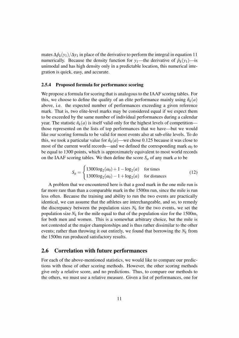
2.5.4 Proposed formula for performance scoring

We propose a formula for scoring that is analogous to the IAAF scoring tables. Forthis, we choose to define the quality of an elite performance mainly using nk(a)above, i.e. the expected number of performances exceeding a given referencemark. That is, two elite-level marks may be considered equal if we expect themto be exceeded by the same number of individual performances during a calendaryear. The statistic nk(a) is itself valid only for the highest levels of competition—those represented on the lists of top performances that we have—but we wouldlike our scoring formula to be valid for most events also at sub-elite levels. To dothis, we took a particular value for nk(a)—we chose 0.125 because it was close tomost of the current world records—and we defined the corresponding mark a0 tobe equal to 1300 points, which is approximately equivalent to most world recordson the IAAF scoring tables. We then define the score Sa of any mark a to be

Sa =

{1300log2(a0)+1− log2(a) for times

1300log2(a0)−1+ log2(a) for distances(12)

A problem that we encountered here is that a good mark in the one mile run isfar more rare than than a comparable mark in the 1500m run, since the mile is runless often. Because the training and ability to run the two events are practicallyidentical, we can assume that the athletes are interchangeable, and so, to remedythe discrepancy between the population sizes Nk for the two events, we set thepopulation size Nk for the mile equal to that of the population size for the 1500m,for both men and women. This is a somewhat arbitrary choice, but the mile isnot contested at the major championships and is thus rather dissimilar to the otherevents; rather than throwing it out entirely, we found that borrowing the Nk fromthe 1500m run produced satisfactory results.

2.6 Correlation with future performancesFor each of the above-mentioned statistics, we would like to compare our predic-tions with those of other scoring methods. However, the other scoring methodsgive only a relative score, and no predictions. Thus, to compare our methods tothe others, we must use a relative measure. Given a list of performances, one for

11

each athletic event, we assign scores to each mark and then calculate the Pear-son correlation coefficient between the scores and some future outcome, eitherthe number of better performances for each event or the improvement in perfor-mance over some reference mark. For the purposes of comparing with the IAAFscoring tables, we define “improvement in performance” of a new mark anew overan old mark aold to be − log(anew/aold). This gives a measure of the relativeimprovement, which could be negative if the new mark is worse than the oldmark. As above, we use the inverse of this score for events in which a highermark is better. The expected relative improvement is another estimate of thequality of a given performance. Below, we use as reference performances aoldthe 10th, 25th, 50th, and 100th best all-time performances prior to the analysisyear (2000, 2008, or 2012).

For example, for the year 2000 analysis, we calculate the expected best per-formance x1 over the next two years (2000-2001) and we let this be anew whilethe 10th, 25th, 50th, and 100th best performances prior to 2000 are each usedas aold . This gives four different versions of the expected improvement score foreach athletic event for each analysis year, for which we can then calculate a Pear-son correlation with actual performances in those subsequent years. If an aold fora particular event is weaker than that of other events, we expect to see a larger im-provement in subsequent years, and likewise a smaller improvement for strongerreference performances aold .

Below, we list many such correlations for our scoring methods, and we com-pare them with correlations for the IAAF scoring tables.

3 ResultsIn this section, we give three sets of results: one for data preceding 2000, which wecompare with later performances; one for data preceding 2008, which we comparewith later performances as well as to the 2008 IAAF scoring tables; and one fordata up to the present day (1 October 2011), which we use to make predictions forthe coming years.

3.1 ConvergenceFor the three time periods, 2000, 2008, and 2012, and for each of these using allprior data and then only five years of data (thus, six cases in total), the MCMCsampling converged usually without using the empirical prior on the total popula-tion size. The slowest convergence in general occurred when using five years ofdata prior to 2008. Only 37 out of 48 events had Gelman-Rubin diagnostic statis-tics less than 1.1. When using the empirical prior, the Gelman-Rubin diagnostic

12

was less than 1.1 for every event in every case, and in each case was less than 1.05for at least 43 of the 48 events.

Population sizes varied between the events, and the use of the empirical prioron Nk improved convergence and moderated unreasonable population sizes. Forexample, for all data preceding 2008, the median population size was 19,028,and the robust standard deviation (using 75% of the events) of log(Nk) was 2.93.The smallest (unrestricted) estimated population size was 510.4 for the women’smile run, and the largest was 2.71× 1016 for men’s pole vault. Large populationsizes such as that of the men’s pole vault are clearly too large, and thus usingthe empirical prior makes intuitive sense as well as improves convergence. Theestimated population size for men’s pole vault when using the empirical prior wasstill 38.0 million (3.8× 107), and that of the women’s mile run was 1309.9, sosome flexibility in the choice of population sizes was preserved.

A set of selected posterior expectations of parameter values are shown in ta-ble 1. Fans of track and field will notice that the marks eµk are rather mediocrefor elite athletes, and those events with larger estimated population sizes have lessimpressive values for eµk , which makes sense intuitively. Assuming that the verybest athletes are always participating in their respective events, a larger populationsize indicates that there are more less-talented athletes participating and makingthe average performance weaker.

3.2 Predictions made prior to 2000We used data from before 2000 to predict both the number of performances ex-ceeding and the expected improvement over four different reference marks in eachevent, namely the 10th, 25th, 50th, and 100th best ever marks in each event at theend of 1999. The Pearson correlations of our predictions with the actual outcomesin the subsequent 12 years can be seen in tables 2 and 3.

We can see in table 2 that the predicted number of better performances corre-lates much more highly with the actual outcomes when we used only the previousfive years of data. In fact, the predictions using all data had very poor correla-tion (Pearson) with the actual outcomes, but the same is not true of the predictedperformance improvement. The predicted improvements were significantly corre-lated with the actual improvements both when we used all data and when we usedonly the previous five years of data, though the latter still gives better results. Wesuspect that that the total number of athletes participating in the various eventshas changed more dramatically over time than has the quality of the very bestperformers, making our predictions of best performances—and the associated im-provement score over the reference marks—more accurate than our predictions ofnumbers of athletes exceeding the same reference mark.

Table 4 gives the Pearson correlation of the predicted probabilities of a world

13

Event eµk−2σk eµk eµk+2σk E[Nk]mens100m 10.55 11.28 12.05 1371048mens200m 21.76 23.66 25.72 1543952mens1500m 3:32.22 3:38.78 3:45.55 2469mensMarathon 2:05:55.76 2:11:13.44 2:16:44.49 1284mensHJ 2.00 2.11 2.22 695184mensLJ 6.30 6.96 7.68 326672womens100m 11.33 12.01 12.73 83707womens200m 23.32 24.75 26.27 146548womens1500m 3:59.52 4:05.33 4:11.29 625womensMarathon 2:22:38.28 2:29:23.24 2:36:27.37 823womensHJ 1.69 1.82 1.96 11229womensLJ 5.53 6.00 6.51 174252

Table 1: Examples of fitted distributions. Shown here are a few summaries ofselected fitted distributions. In the rightmost four columns, we give the log-normalequivalent of a normal distribution’s (1) mean minus two standard deviations (i.e.eµk−2σk), (2) the mean, and (3) mean plus two standard deviations, as well as (4)the posterior expectation of the total population size. Running times are given inhours:minutes:seconds, where applicable, distances and heights are given in me-ters, and population sizes are the number of performances in the five-year period2007-2011.

years using all prior data using 5 years of prior data10th 25th 50th 100th 10th 25th 50th 100th

2000-2001 -0.185 -0.139 -0.118 0.090 0.226 0.414 0.498 0.6122000-2003 -0.198 -0.095 -0.100 0.062 0.163 0.380 0.463 0.5812000-2005 -0.175 -0.082 -0.094 0.050 0.139 0.352 0.423 0.5722000-2007 -0.164 -0.082 -0.096 0.049 0.124 0.331 0.397 0.5542000-2009 -0.161 -0.085 -0.097 0.051 0.117 0.323 0.388 0.5482000-2011 -0.158 -0.085 -0.097 0.049 0.116 0.319 0.382 0.552

Table 2: Correlations, 2000 number of better performances. Given in thetable are the Pearson correlation coefficients between the predicted and actualnumber of performances exceeding a reference mark, based on the year 2000.The reference marks (the columns) are the 10th, 25th, 50th, and 100th best priormark in each event.

record being set with the actual outcome (1 for a world record, 0 for none) over agiven time period. Again, there is significant correlation between the predictionsand the outcomes, and the predictions based on five years of data were generally

14

years using all prior data using 5 years of prior data10th 25th 50th 100th 10th 25th 50th 100th

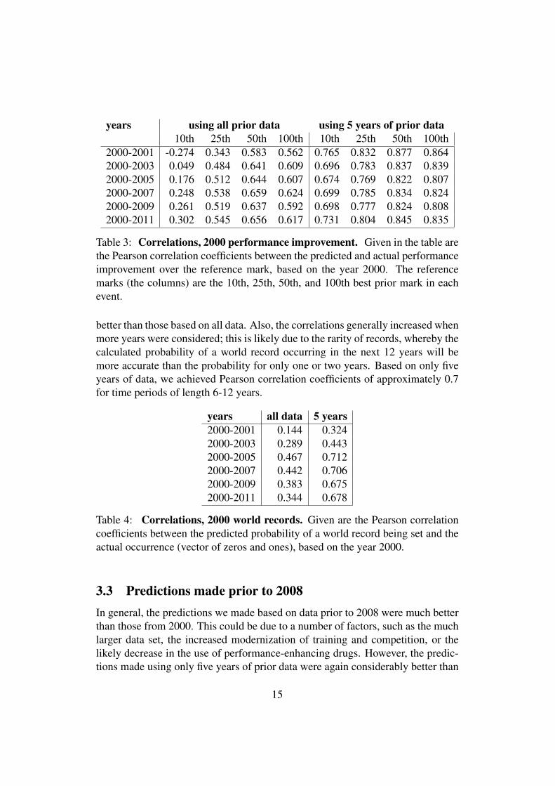
2000-2001 -0.274 0.343 0.583 0.562 0.765 0.832 0.877 0.8642000-2003 0.049 0.484 0.641 0.609 0.696 0.783 0.837 0.8392000-2005 0.176 0.512 0.644 0.607 0.674 0.769 0.822 0.8072000-2007 0.248 0.538 0.659 0.624 0.699 0.785 0.834 0.8242000-2009 0.261 0.519 0.637 0.592 0.698 0.777 0.824 0.8082000-2011 0.302 0.545 0.656 0.617 0.731 0.804 0.845 0.835

Table 3: Correlations, 2000 performance improvement. Given in the table arethe Pearson correlation coefficients between the predicted and actual performanceimprovement over the reference mark, based on the year 2000. The referencemarks (the columns) are the 10th, 25th, 50th, and 100th best prior mark in eachevent.

better than those based on all data. Also, the correlations generally increased whenmore years were considered; this is likely due to the rarity of records, whereby thecalculated probability of a world record occurring in the next 12 years will bemore accurate than the probability for only one or two years. Based on only fiveyears of data, we achieved Pearson correlation coefficients of approximately 0.7for time periods of length 6-12 years.

years all data 5 years2000-2001 0.144 0.3242000-2003 0.289 0.4432000-2005 0.467 0.7122000-2007 0.442 0.7062000-2009 0.383 0.6752000-2011 0.344 0.678

Table 4: Correlations, 2000 world records. Given are the Pearson correlationcoefficients between the predicted probability of a world record being set and theactual occurrence (vector of zeros and ones), based on the year 2000.

3.3 Predictions made prior to 2008In general, the predictions we made based on data prior to 2008 were much betterthan those from 2000. This could be due to a number of factors, such as the muchlarger data set, the increased modernization of training and competition, or thelikely decrease in the use of performance-enhancing drugs. However, the predic-tions made using only five years of prior data were again considerably better than

15

those using all prior data. In fact, our predictions of both the number of perfor-mances exceeding and the relative improvement over the 100th best performancesof all time have Pearson correlations greater than 0.83 with the actual outcomes inthe 2008 athletics season as well as for all seasons through 2011. Tables 5 and 6show the details of the correlation coefficients.

year(s) using all prior data using 5 years of prior data10th 25th 50th 100th 10th 25th 50th 100th

2008 0.322 0.330 0.294 0.193 0.561 0.765 0.774 0.8412008-2009 0.329 0.298 0.298 0.197 0.672 0.752 0.784 0.8342008-2010 0.333 0.299 0.331 0.206 0.602 0.728 0.783 0.8312008-2011 0.321 0.308 0.345 0.210 0.605 0.751 0.806 0.847

Table 5: Correlations, 2008 number of better performances. Given in thetable are the Pearson correlation coefficients between the predicted and actualnumber of performances exceeding a reference mark, based on the year 2008.The reference marks (the columns) are the 10th, 25th, 50th, and 100th best priormark in each event.

year(s) using all prior data using 5 years of prior data10th 25th 50th 100th 10th 25th 50th 100th

2008 0.188 0.129 0.249 0.286 0.825 0.821 0.830 0.8352008-2009 0.110 0.064 0.191 0.260 0.847 0.842 0.849 0.8512008-2010 0.038 0.042 0.181 0.260 0.846 0.841 0.849 0.8532008-2011 0.030 0.068 0.214 0.298 0.837 0.836 0.847 0.853

Table 6: Correlations, 2008 performance improvement. Given in the table arethe Pearson correlation coefficients between the predicted and actual performanceimprovement over the reference mark, based on the year 2008. The referencemarks (the columns) are the 10th, 25th, 50th, and 100th best prior mark in eachevent.

Table 7 shows the Pearson correlation between predicted probabilities of worldrecord being set and the actual outcomes. For the period 2008-2011, the predictedprobabilities had a correlation coefficient of 0.48 with the actual outcomes, whichis slightly higher than the corresponding correlation coefficient from the four-yearperiod beginning in 2000, as shown in table 4. Thus, our predictions from thebeginning of the year 2008 are better in nearly every case than those from theyear 2000.

16

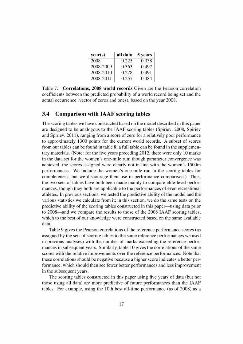
year(s) all data 5 years2008 0.225 0.3382008-2009 0.363 0.4972008-2010 0.278 0.4912008-2011 0.257 0.484

Table 7: Correlations, 2008 world records Given are the Pearson correlationcoefficients between the predicted probability of a world record being set and theactual occurrence (vector of zeros and ones), based on the year 2008.

3.4 Comparison with IAAF scoring tablesThe scoring tables we have constructed based on the model described in this paperare designed to be analogous to the IAAF scoring tables (Spiriev, 2008, Spirievand Spiriev, 2011), ranging from a score of zero for a relatively poor performanceto approximately 1300 points for the current world records. A subset of scoresfrom our tables can be found in table 8; a full table can be found in the supplemen-tary materials. (Note: for the five years preceding 2012, there were only 10 marksin the data set for the women’s one-mile run; though parameter convergence wasachieved, the scores assigned were clearly not in line with the women’s 1500mperformances. We include the women’s one-mile run in the scoring tables forcompleteness, but we discourage their use in performance comparison.) Thus,the two sets of tables have both been made mainly to compare elite-level perfor-mances, though they both are applicable to the performances of even recreationalathletes. In previous sections, we tested the predictive ability of the model and thevarious statistics we calculate from it; in this section, we do the same tests on thepredictive ability of the scoring tables constructed in this paper—using data priorto 2008—and we compare the results to those of the 2008 IAAF scoring tables,which to the best of our knowledge were constructed based on the same availabledata.

Table 9 gives the Pearson correlations of the reference performance scores (asassigned by the sets of scoring tables to the same reference performances we usedin previous analyses) with the number of marks exceeding the reference perfor-mances in subsequent years. Similarly, table 10 gives the correlations of the samescores with the relative improvements over the reference performances. Note thatthese correlations should be negative because a higher score indicates a better per-formance, which should then see fewer better performances and less improvementin the subsequent years.

The scoring tables constructed in this paper using five years of data (but notthose using all data) are more predictive of future performances than the IAAFtables. For example, using the 10th best all-time performance (as of 2008) as a

17

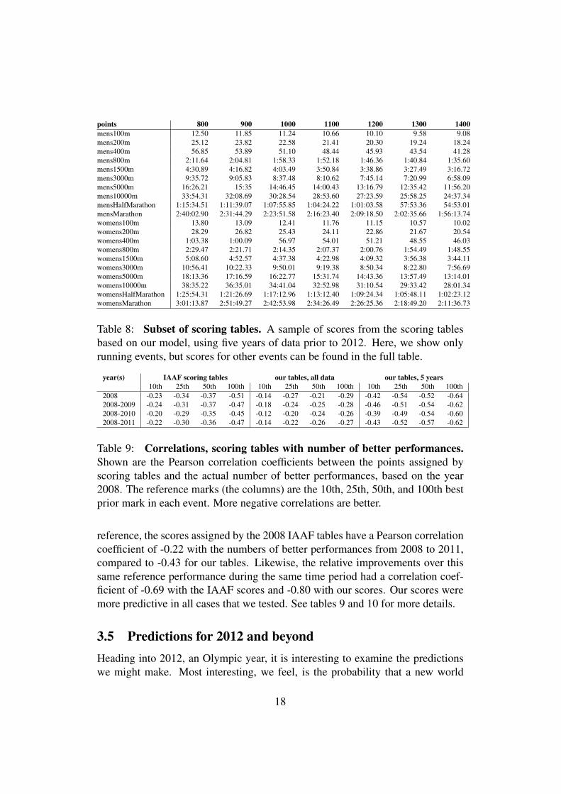
points 800 900 1000 1100 1200 1300 1400mens100m 12.50 11.85 11.24 10.66 10.10 9.58 9.08mens200m 25.12 23.82 22.58 21.41 20.30 19.24 18.24mens400m 56.85 53.89 51.10 48.44 45.93 43.54 41.28mens800m 2:11.64 2:04.81 1:58.33 1:52.18 1:46.36 1:40.84 1:35.60mens1500m 4:30.89 4:16.82 4:03.49 3:50.84 3:38.86 3:27.49 3:16.72mens3000m 9:35.72 9:05.83 8:37.48 8:10.62 7:45.14 7:20.99 6:58.09mens5000m 16:26.21 15:35 14:46.45 14:00.43 13:16.79 12:35.42 11:56.20mens10000m 33:54.31 32:08.69 30:28.54 28:53.60 27:23.59 25:58.25 24:37.34mensHalfMarathon 1:15:34.51 1:11:39.07 1:07:55.85 1:04:24.22 1:01:03.58 57:53.36 54:53.01mensMarathon 2:40:02.90 2:31:44.29 2:23:51.58 2:16:23.40 2:09:18.50 2:02:35.66 1:56:13.74womens100m 13.80 13.09 12.41 11.76 11.15 10.57 10.02womens200m 28.29 26.82 25.43 24.11 22.86 21.67 20.54womens400m 1:03.38 1:00.09 56.97 54.01 51.21 48.55 46.03womens800m 2:29.47 2:21.71 2:14.35 2:07.37 2:00.76 1:54.49 1:48.55womens1500m 5:08.60 4:52.57 4:37.38 4:22.98 4:09.32 3:56.38 3:44.11womens3000m 10:56.41 10:22.33 9:50.01 9:19.38 8:50.34 8:22.80 7:56.69womens5000m 18:13.36 17:16.59 16:22.77 15:31.74 14:43.36 13:57.49 13:14.01womens10000m 38:35.22 36:35.01 34:41.04 32:52.98 31:10.54 29:33.42 28:01.34womensHalfMarathon 1:25:54.31 1:21:26.69 1:17:12.96 1:13:12.40 1:09:24.34 1:05:48.11 1:02:23.12womensMarathon 3:01:13.87 2:51:49.27 2:42:53.98 2:34:26.49 2:26:25.36 2:18:49.20 2:11:36.73

Table 8: Subset of scoring tables. A sample of scores from the scoring tablesbased on our model, using five years of data prior to 2012. Here, we show onlyrunning events, but scores for other events can be found in the full table.

year(s) IAAF scoring tables our tables, all data our tables, 5 years10th 25th 50th 100th 10th 25th 50th 100th 10th 25th 50th 100th

2008 -0.23 -0.34 -0.37 -0.51 -0.14 -0.27 -0.21 -0.29 -0.42 -0.54 -0.52 -0.642008-2009 -0.24 -0.31 -0.37 -0.47 -0.18 -0.24 -0.25 -0.28 -0.46 -0.51 -0.54 -0.622008-2010 -0.20 -0.29 -0.35 -0.45 -0.12 -0.20 -0.24 -0.26 -0.39 -0.49 -0.54 -0.602008-2011 -0.22 -0.30 -0.36 -0.47 -0.14 -0.22 -0.26 -0.27 -0.43 -0.52 -0.57 -0.62

Table 9: Correlations, scoring tables with number of better performances.Shown are the Pearson correlation coefficients between the points assigned byscoring tables and the actual number of better performances, based on the year2008. The reference marks (the columns) are the 10th, 25th, 50th, and 100th bestprior mark in each event. More negative correlations are better.

reference, the scores assigned by the 2008 IAAF tables have a Pearson correlationcoefficient of -0.22 with the numbers of better performances from 2008 to 2011,compared to -0.43 for our tables. Likewise, the relative improvements over thissame reference performance during the same time period had a correlation coef-ficient of -0.69 with the IAAF scores and -0.80 with our scores. Our scores weremore predictive in all cases that we tested. See tables 9 and 10 for more details.

3.5 Predictions for 2012 and beyondHeading into 2012, an Olympic year, it is interesting to examine the predictionswe might make. Most interesting, we feel, is the probability that a new world

18

year(s) IAAF scoring tables our tables, all data our tables, 5 years10th 25th 50th 100th 10th 25th 50th 100th 10th 25th 50th 100th

2008 -0.65 -0.66 -0.68 -0.69 0.02 -0.06 -0.18 -0.28 -0.77 -0.77 -0.78 -0.802008-2009 -0.68 -0.69 -0.71 -0.72 0.06 -0.02 -0.14 -0.24 -0.78 -0.78 -0.79 -0.802008-2010 -0.68 -0.68 -0.71 -0.71 0.07 -0.01 -0.14 -0.24 -0.79 -0.79 -0.80 -0.812008-2011 -0.69 -0.69 -0.71 -0.72 0.05 -0.04 -0.18 -0.28 -0.80 -0.80 -0.81 -0.83

Table 10: Correlations, scoring tables with performance improvement.Shown are the Pearson correlation coefficients between the points assignedby scoring tables and the actual performance improvements over the refer-ence mark, based on the year 2008. The reference marks (the columns) arethe 10th, 25th, 50th, and 100th best prior mark in each event. More negativecorrelations are better.

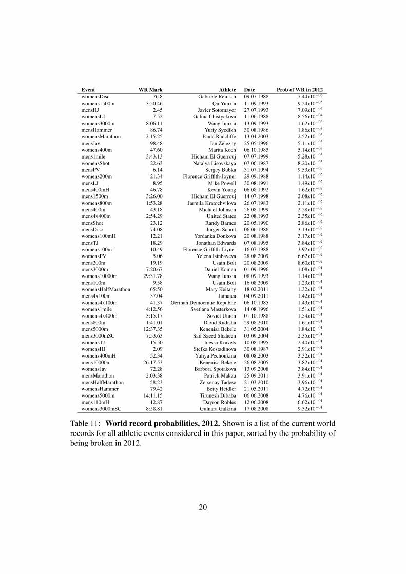
record is set. Thus, we have compiled in table 11 all of the current world recordsand we have sorted them by probability of being broken in 2012.

The probabilities range from less than 1/100,000 for women’s discus to al-most certain (0.95) for women’s steeplechase. Most of the world records (26 outof 48) have less than a 10% chance of being broken, a quarter (12) have less thana 1% chance, and only two—women’s steeplechase and men’s 110m hurdles—are likely to get broken. In both of these events, the world record was set recently,in 2008 in both cases, and there are many other recent marks that come close tothe record. In particular, there are nine women’s steeplechase performances fromthe past five years that are within ten seconds of the world record, including therecord itself. There are seven marks (including the record) in the men’s 110m hur-dles from the past five five years that are within 0.05s of the world record. Thissuggests that in both of these events, with so many recent marks that are close tothe record, it is more likely than not that a record will be set in 2012.

On the other end of the spectrum, those records least likely to get broken aresome of the older records, with only 6 of the 25 toughest (according to table 11)records occurring in the past 15 years, whereas 17 of the 25 weakest records haveoccurred in the past 15 years. In the women’s discus, where the record is leastlikely to get broken, no one has produced a mark in the top 100 in nearly 20 years.The women’s 1500m run, which has the second toughest record, has seen no timewithin five seconds of the record in over ten years.

Notably, two events, the one mile run and the 3000m run (non-Olympic events),are contested less frequently than the rest, and therefore the probabilities of theirrecords being broken are lower than if they were contested more often. For in-stance, the men’s one mile world record is obviously—to any track and fieldfan—easier for a well-trained athlete to break than the 1500m world record, butthe probability of the mile record actually being broken is lower since there arefar fewer attempts.

19

Event WR Mark Athlete Date Prob of WR in 2012womensDisc 76.8 Gabriele Reinsch 09.07.1988 7.44x10−06

womens1500m 3:50.46 Qu Yunxia 11.09.1993 9.24x10−05

mensHJ 2.45 Javier Sotomayor 27.07.1993 7.09x10−04

womensLJ 7.52 Galina Chistyakova 11.06.1988 8.56x10−04

womens3000m 8:06.11 Wang Junxia 13.09.1993 1.62x10−03

mensHammer 86.74 Yuriy Syedikh 30.08.1986 1.86x10−03

womensMarathon 2:15:25 Paula Radcliffe 13.04.2003 2.52x10−03

mensJav 98.48 Jan Zelezny 25.05.1996 5.11x10−03

womens400m 47.60 Marita Koch 06.10.1985 5.14x10−03

mens1mile 3:43.13 Hicham El Guerrouj 07.07.1999 5.28x10−03

womensShot 22.63 Natalya Lisovskaya 07.06.1987 8.20x10−03

mensPV 6.14 Sergey Bubka 31.07.1994 9.53x10−03

womens200m 21.34 Florence Griffith-Joyner 29.09.1988 1.14x10−02

mensLJ 8.95 Mike Powell 30.08.1991 1.49x10−02

mens400mH 46.78 Kevin Young 06.08.1992 1.62x10−02

mens1500m 3:26.00 Hicham El Guerrouj 14.07.1998 2.08x10−02

womens800m 1:53.28 Jarmila Kratochvilova 26.07.1983 2.11x10−02

mens400m 43.18 Michael Johnson 26.08.1999 2.28x10−02

mens4x400m 2:54.29 United States 22.08.1993 2.35x10−02

mensShot 23.12 Randy Barnes 20.05.1990 2.86x10−02

mensDisc 74.08 Jurgen Schult 06.06.1986 3.13x10−02

womens100mH 12.21 Yordanka Donkova 20.08.1988 3.17x10−02

mensTJ 18.29 Jonathan Edwards 07.08.1995 3.84x10−02

womens100m 10.49 Florence Griffith-Joyner 16.07.1988 3.92x10−02

womensPV 5.06 Yelena Isinbayeva 28.08.2009 6.62x10−02

mens200m 19.19 Usain Bolt 20.08.2009 8.60x10−02

mens3000m 7:20.67 Daniel Komen 01.09.1996 1.08x10−01

womens10000m 29:31.78 Wang Junxia 08.09.1993 1.14x10−01

mens100m 9.58 Usain Bolt 16.08.2009 1.23x10−01

womensHalfMarathon 65:50 Mary Keitany 18.02.2011 1.32x10−01

mens4x100m 37.04 Jamaica 04.09.2011 1.42x10−01

womens4x100m 41.37 German Democratic Republic 06.10.1985 1.43x10−01

womens1mile 4:12.56 Svetlana Masterkova 14.08.1996 1.51x10−01

womens4x400m 3:15.17 Soviet Union 01.10.1988 1.54x10−01

mens800m 1:41.01 David Rudisha 29.08.2010 1.61x10−01

mens5000m 12:37.35 Kenenisa Bekele 31.05.2004 1.84x10−01

mens3000mSC 7:53.63 Saif Saeed Shaheen 03.09.2004 2.35x10−01

womensTJ 15.50 Inessa Kravets 10.08.1995 2.40x10−01

womensHJ 2.09 Stefka Kostadinova 30.08.1987 2.91x10−01

womens400mH 52.34 Yuliya Pechonkina 08.08.2003 3.32x10−01

mens10000m 26:17.53 Kenenisa Bekele 26.08.2005 3.82x10−01

womensJav 72.28 Barbora Spotakova 13.09.2008 3.84x10−01

mensMarathon 2:03:38 Patrick Makau 25.09.2011 3.91x10−01

mensHalfMarathon 58:23 Zersenay Tadese 21.03.2010 3.96x10−01

womensHammer 79.42 Betty Heidler 21.05.2011 4.72x10−01

womens5000m 14:11.15 Tirunesh Dibaba 06.06.2008 4.76x10−01

mens110mH 12.87 Dayron Robles 12.06.2008 6.62x10−01

womens3000mSC 8:58.81 Gulnara Galkina 17.08.2008 9.52x10−01

Table 11: World record probabilities, 2012. Shown is a list of the current worldrecords for all athletic events considered in this paper, sorted by the probability ofbeing broken in 2012.

20

4 DiscussionThis paper has been an attempt to rigorously quantify what it means for an athleticperformance to be “good”, and, alternatively, what it means for a performanceto be better than another performance, particularly if the two performances arein different events. We use primarily two alternative reasons why an observerof track and field might believe that a performance is good, restated from theintroduction:

1. A performance is good if few athletes improve upon it, or

2. A performance is good if it is close to or improves upon the [previous] bestperformance.

In the introduction, we suggested that the 9.58s 100m dash that Usain Boltran in the 2009 World Champtionships might be one of the greatest athletics featsever. But, we can see in table 11 that there are many records that are less likelyto be broken next year than Usain Bolt’s 9.58s. In fact, his own 200m worldrecord (19.19) is one of them. On the other hand, of the world records that wereset since the year 2000 (18 of them), these are the third and fourth least likelyto be broken, so perhaps they are so impressive because they are among the bestrecords of recent memory.

In addition to calculating probabilities of world records, we also calculatedexpected number of performances improving upon a given mark, expected bestperformances, and a set of scoring tables intended to be analagous to the IAAFscoring tables. Our results, particularly tables 9 and 10, show that our model canpredict the levels of future performances with considerable success, and betterthan the most common method of performance scoring, the IAAF scoring tables.Given a set of performances or records, we can predict which ones will be broken,how many times, and by how much, and these predictions have a Pearson correla-tion coefficient of over 0.8 in many cases with actual future outcomes. Our scoringtables, which are derived from the expected number of annual performances ex-ceeding a given mark, outperformed the IAAF scoring tables for two differentprediction types, each with four sets of reference marks and four time periods,giving 32 cases wherein our predictions correlated more highly in every case.

The keys to the success, we believe, are the large amount of data used in modelfitting and the probabilistic approach. Past scoring methods typically have used afixed number of top performances—in some cases very few—such as the top tenor one hundred within a particular time period; we wanted to avoid this restric-tion and use all available data to compute actual probabilities. In general, moredata is better, though admittedly there were some outlying circumstances in thepast when, for example, performance enhancing drugs have been used without

21

detection, or marks were set under other questionable circumstances. One glaringexample of this is the fact that no woman has produced a top-100 mark in the shotput or the discus in the past ten years. Likely because of these questionable per-formances, we have found that the most accurate way to predict the performancesof the next year is by fitting the model only to recent data. Another example of anegative shift in performance is the recent switch to all-women road races, partic-ularly in the marathon. Paula Radcliffe’s marathon world record is one of the bestmarks in athletics, but it was set with men running alongside the women. It hasbeen ruled (by the IAAF) that mixed-sex races are no longer eligible for women’srecords, but it seems that previous marks will be allowed to stand. Though notpreviously considered cheating, male pacers can help women significantly, andin their absence we have indeed seen a drop in the quality of women’s marathontimes, as most major marathons have in the past few years switched to separatemen’s and women’s races. These shifts in performance level are a problem wemight address in future research. It is reasonable to assume that performancelevels improve over time due to improved training and technique, and any large-scale decline is the result of a reduction in the prevalence of performance enhanc-ing drugs or other forms of performance aid or cheating. There are a number ofways we might detect and remove—or otherwise take into account—these ques-tionable performances, possibly using robust statistics or parameter optimizationtechniques. In addition, other probability distributions might also be considered ifthey seem to fit the data.

In a more general sense, it would likely help the predictive ability of the modelif time were included as a contributing variable. Modeling general performancechanges over time would give us further abilities to discuss and describe the his-tory of athletics, such as in detecting or predicting eras of great improvement orchange and also in modeling the maturity of a event, in the sense that, for exam-ple, the women’s steeplechase isn’t quite mature yet since it has been an Olympicevent since only 2008 and its records still fall quite often.

Lastly, the type of analysis demonstrated in this paper need not be limited toathletics. Any standardized competition with a large number of performances thatare either normally or log-normally distributed can be modeled in this way. Swim-ming and rowing come to mind, though those are more dependent on technologythan athletics and thus may be more difficult to model. All in all, a probabilisticapproach to studying sports performances seems to be a practical and valuabletool in examining the history and predicting the future of sport.

22

ReferencesCameron, D. F. (1998): “Time equivalence model,” web page, URL http://www.

cs.uml.edu/~phoffman/cammod.html, accessed on 2011.10.01.

Daniels, J. and J. Gilbert (1979): Oxygen Power: Performance Tables for DistanceRunners, J Daniels and J Gilbert.

Gardner, J. and J. Purdy (1970): “Computer generated track scoring tables,”Medicine and science in sports, 2, 152–161.

Gelman, A. and D. B. Rubin (1992): “Inference from iterative simulation usingmultiple sequences,” Statistical Science, 7, 457–472.

Geyer., C. J. (2010): mcmc: Markov Chain Monte Carlo, URL http://CRAN.

R-project.org/package=mcmc, r package version 0.8.

Hastings, W. (1970): “Monte carlo sampling methods using markov chainsand their applications,” Biometrika, 57, 97–109, URL http://biomet.

oxfordjournals.org/content/57/1/97.abstract.

International Association of Athletics Federations (2001): “IAAF scoring ta-bles for combined events,” pdf document, URL http://www.iaaf.org/

competitions/technical/scoringtables/index.html.

Larsson, P. (2011): “Alltime-athletics.com,” Web site, URL http://

alltime-athletics.com, data as of 2011.10.01.

MacKay, D. J. C. (1999): “Comparison of approximate methods for handlinghyperparameters,” Neural Computation, 11, 1035–1068.

McMillan, G. (2011): “The McMillan running calculator,” Web page, URL http:

//www.mcmillanrunning.com/mcmillanrunningcalculator.htm.

Plummer, M., N. Best, K. Cowles, and K. Vines (2006): “Coda: Convergencediagnosis and output analysis for mcmc,” R News, 6, 7–11, URL http:

//CRAN.R-project.org/doc/Rnews/.

R Development Core Team (2008): R: A language and environment for statisticalcomputing, R Foundation for Statistical Computing, Vienna, Austria, URLhttp://www.R-project.org, ISBN 3-900051-07-0.

Riegel, P. (1977): “Time predicting,” Runner’s World.

Spiriev, B. (2008): “IAAF scoring tables of athletics: 2008 revised edi-

23

tion,” pdf document, URL http://www.iaaf.org/mm/Document/

Competitions/TechnicalArea/ScoringOutdoor2008_742.pdf.

Spiriev, B. and A. Spiriev (2011): “IAAF scoring tables of athletics: 2011 revisededition,” pdf document, URL http://www.iaaf.org/competitions/

technical/scoringtables/index.html.

24