Comparative Evaluation of Discrete-Time Dynamic Models of TCSC

S. R. Joshi, A. M. KulkarniIndian Institute of Technology Bombay

Mumbai, Indiasrjoshi@iitb.ac.in, anil@ee.iitb.ac.in

Abstract - This paper presents a comparative evalua-tion of linearized discrete-time models of TCSC. The mod-els considered are modular, use six samples per cycle andare sample-invariant. Two different techniques to interfaceTCSC model with the rest of the system are compared: onein which the discrete TCSC model is interfaced with the dis-cretized model of the rest of the system, and the other inwhich the TCSC is converted into an equivalent continuoustime model and interfaced with the continuous model of therest of the system. The result of eigen-analysis using thesemodels is compared with detailed digital simulation. Casestudies involving open and closed loop control of TCSC andSSR are presented. The discrete-time model with linear vari-ation of interface variables is found to give good accuracy un-der all tested situations, whereas maintaining interface vari-ables constant in a sampling interval can give incorrect in-formation of the stability of super-synchronous network orTCSC modes.

Keywords - TCSC, Dynamic Modeling, Discrete-TimeSystems

1 Introduction

ANALYSIS of Thyristor Controlled Series Compen-sator (TCSC), i.e., its effect on the stability of net-

work, torsional and controller modes, requires an accu-rate model of the dynamic system. While the nonlinearequations of a power system and time variant equationsof TCSC can be handled by a simulation program, tech-niques like eigen-analysis are useful and insightful, espe-cially for design and parameter sensitivity studies. There-fore, attempts have been made in the past to obtain lin-earized models suitable for eigen-analysis.Ghosh and Ledwich [1], Rajaraman et al [2] and Jalali etal ( [3] and [4]) have presented analytical discrete-timemodels of TCSC based on Poincare mapping technique.However these models are not modular, i.e., the TCSCmodel cannot be derived independent of the rest of thesystem and subsequently interfaced with it. Othman andAngquist [5] overcame this difficulty by approximatingthe line current to be constant in the half cycle intervalin between the samples.A higher bandwidth discrete-time model using six-samples per cycle was obtained in [6]. However, thisdiscrete-time model is not modular and requires numeri-cal computation of the state transition matrix. The modelis also sample variant and yields periodically varying dis-crete state space matrices. Therefore, a “lifting” techniquewas used to analyze this model.

Sample invariance and modularity can be introduced inthe six-sample per cycle model by using a sample vari-ant transformation in the discrete domain, as given in [7],and by assuming that the interface variables (line currentand TCSC voltage) are constant in a sampling interval [5].Further refinement made in this paper by assuming a lin-ear variation of interface variables.Two different techniques can be used to interface TCSCmodel with the rest of the system: one in which the dis-crete TCSC model is interfaced with the discretized modelof the rest of the system, and the other in which the TCSCis converted into an equivalent continuous time model andinterfaced with the continuous model of the rest of thesystem. These techniques involve some approximationsregarding the behavior of the interface variables and thezero-sequence components. Hence there is a need to crit-ically analyze the effect of these methods to introducemodularity.This paper presents a comparative assessment of threevariants of six-sample-per cycle modular TCSC models.The studies done in this paper also incorporate the ef-fects of a current synchronized Phase Locked Loop (PLL),TCSC voltage controller, and generator turbine shaft dy-namics. The results obtained are tested against those ob-tained by detailed digital simulation. An important fea-ture of this paper is that the accuracy of these modelsis tested by a quantitative comparison of the predictedcontroller instability gains and the frequency/damping ofdominant modes. Eigen-analysis of a TCSC compensatedline for Subsynchronous Resonance (SSR) studies usingthese models is also done and the critical torsional modesand their decrement factor is predicted and validated. Thediscrete-time model with linear variation of interface vari-ables is found to give good accuracy under all tested situa-tions, whereas maintaining interface variables constant ina sampling interval can give incorrect information of thestability of super-synchronous TCSC or network modes.

2 TCSC Model

LaT

v

ii

Thyristor Strings

C

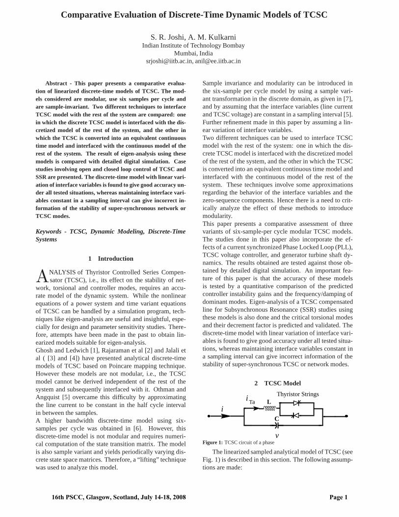
Figure 1: TCSC circuit of a phase

The linearized sampled analytical model of TCSC (seeFig. 1) is described in this section. The following assump-tions are made:

16th PSCC, Glasgow, Scotland, July 14-18, 2008 Page 1

1. TCSC is operated in capacitive mode only and theconduction angle of thyristors,σ, is limited to 60electrical degrees. Most TCSCs usually operate inthis range.

2. The thyristors are assumed to be ideal. For simplic-ity, the reactor is assumed to be lossless.

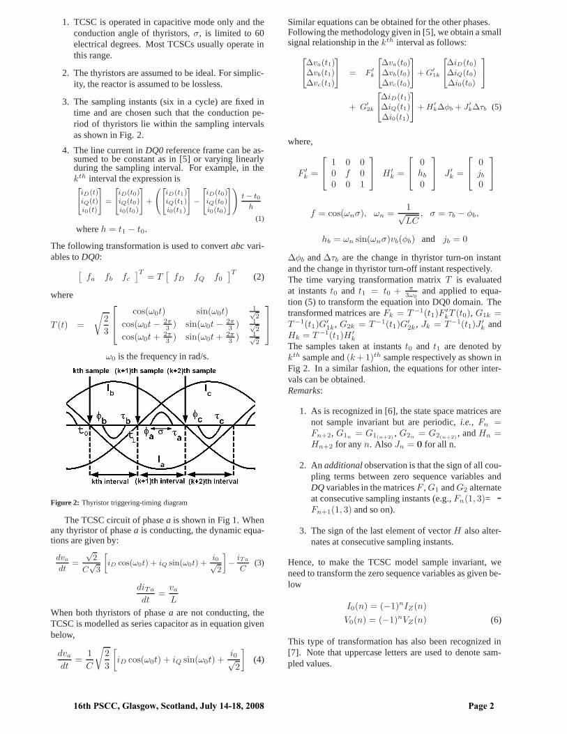
3. The sampling instants (six in a cycle) are fixed intime and are chosen such that the conduction pe-riod of thyristors lie within the sampling intervalsas shown in Fig. 2.

4. The line current inDQ0 reference frame can be as-sumed to be constant as in [5] or varying linearlyduring the sampling interval. For example, in thekth interval the expression is2

4

iD(t)iQ(t)i0(t)

3

5 =

2

4

iD(t0)iQ(t0)i0(t0)

3

5 +

0

@

2

4

iD(t1)iQ(t1)i0(t1)

3

5 −

2

4

iD(t0)iQ(t0)i0(t0)

3

5

1

A

t − t0

h

(1)

whereh = t1 − t0.

The following transformation is used to convertabc vari-ables toDQ0:

[fa fb fc

]T= T

[fD fQ f0

]T(2)

where

T (t) =

√

2

3

cos(ω0t) sin(ω0t)1√2

cos(ω0t − 2π3

) sin(ω0t − 2π3

) 1√2

cos(ω0t + 2π3

) sin(ω0t + 2π3

) 1√2

ω0 is the frequency in rad/s.

Figure 2: Thyristor triggering-timing diagram

The TCSC circuit of phasea is shown in Fig 1. Whenany thyristor of phasea is conducting, the dynamic equa-tions are given by:

dva

dt=

√2

C√

3

»

iD cos(ω0t) + iQ sin(ω0t) +i0√2

–

− iTa

C(3)

diTa

dt=

va

L

When both thyristors of phasea are not conducting, theTCSC is modelled as series capacitor as in equation givenbelow,

dva

dt=

1

C

√

2

3

[

iD cos(ω0t) + iQ sin(ω0t) +i0√2

]

(4)

Similar equations can be obtained for the other phases.Following the methodology given in [5], we obtain a smallsignal relationship in thekth interval as follows:

2

4

∆va(t1)∆vb(t1)∆vc(t1)

3

5 = F′

k

2

4

∆va(t0)∆vb(t0)∆vc(t0)

3

5 + G′

1k

2

4

∆iD(t0)∆iQ(t0)∆i0(t0)

3

5

+ G′

2k

2

4

∆iD(t1)∆iQ(t1)∆i0(t1)

3

5 + H′

k∆φb + J′

k∆τb (5)

where,

F ′k =

1 0 00 f 00 0 1

H ′k =

0hb

0

J ′k =

0jb

0

f = cos(ωnσ), ωn =1√LC

, σ = τb − φb,

hb = ωn sin(ωnσ)vb(φb) and jb = 0

∆φb and∆τb are the change in thyristor turn-on instantand the change in thyristor turn-off instant respectively.The time varying transformation matrixT is evaluatedat instantst0 and t1 = t0 + π

3ω0and applied to equa-

tion (5) to transform the equation into DQ0 domain. Thetransformed matrices areFk = T−1(t1)F

′kT (t0), G1k =

T−1(t1)G′1k, G2k = T−1(t1)G

′2k, Jk = T−1(t1)J

′k and

Hk = T−1(t1)H′k

The samples taken at instantst0 and t1 are denoted bykth sample and(k + 1)th sample respectively as shown inFig 2. In a similar fashion, the equations for other inter-vals can be obtained.Remarks:

1. As is recognized in [6], the state space matrices arenot sample invariant but are periodic,i.e., Fn =Fn+2, G1n

= G1(n+2), G2n

= G2(n+2), andHn =

Hn+2 for anyn. Also Jn = 0 for all n.

2. Anadditional observation is that the sign of all cou-pling terms between zero sequence variables andDQ variables in the matricesF , G1 andG2 alternateat consecutive sampling instants (e.g.,Fn(1, 3)= -Fn+1(1, 3) and so on).

3. The sign of the last element of vectorH also alter-nates at consecutive sampling instants.

Hence, to make the TCSC model sample invariant, weneed to transform the zero sequence variables as given be-low

I0(n) = (−1)nIZ(n)

V0(n) = (−1)nVZ(n) (6)

This type of transformation has also been recognized in[7]. Note that uppercase letters are used to denote sam-pled values.

16th PSCC, Glasgow, Scotland, July 14-18, 2008 Page 2

If we apply this transformation of zero sequence variables,the resultingsample invariant set of equations are:

∆VD(n + 1)∆VQ(n + 1)∆VZ(n + 1)

= F

∆VD(n)∆VQ(n)∆VZ(n)

+ G1

∆ID(n)∆IQ(n)∆IZ(n)

+ G2

∆ID(n + 1)∆IQ(n + 1)∆IZ(n + 1)

+ H∆φ(n)(7)

The sample invariance obtained by using a transformationis elegant and straight-forward as compared to the liftingof alternate samples described in [6]. For eigen-analysis,it obviates the need to choose between (a) neglecting ef-fect of zero sequence variables, (b) using eitherFn orFn+1, and (c)FnFn+1 of the lifted system.The model represented by (7) is denoted asModel A. Ifwe assume that the line current is constant during sam-pling interval as in [5], thenG1 is appropriately modifiedandG2 is set to zero. The obtained TCSC model is de-noted asModel B. Model C is obtained by converting theTCSC Model B into continuous-time model as follows [5]:

2

4

∆VD(t)

∆VQ(t)

∆VZ(t)

3

5 = At

2

4

∆VD(t)∆VQ(t)∆VZ(t)

3

5 + Bt

2

4

∆ID(t)∆IQ(t)∆IZ(t)

3

5 + Et∆φ(t) (8)

where

At =lnFh

, Bt = (F − I)−1AtG,

Et = (F − I)−1AtH and G = G1 + G2

Discrete Time SampleInvariant Model

Model A

(Six Samples/ cycle)

(Six Samples/ cycle)TCSC Model

Linear Time Variant

During Sampling IntervalLinear Variation of current

Discrete Time Sample Invariant Model

Continuous Time Model(Eq. 8)

Model B Model C

During Sampling IntervalCurrent Constant

Figure 3: Derivation of TCSC Model Variants

The derivation of the three models is schematicallyshown in Fig. 3.

3 Computation of Initial Conditions

The linearized discrete and continuous models requireinitial conditions (at equilibrium) of the line current andTCSC voltages at the turn on instants. Considerable sim-plicity is achieved if we assume line current to be sinu-soidal and free of zero sequence components. The follow-ing steps can be used to determine the initial conditions iffiring delay angle (or conduction angle) is given:

1. The fundamental frequency reactance can be ob-tained using the TCSC reactance formula as a func-tion of the delay angle [9].

2. Phasor analysis (a loadflow) of the entire systemcan be done to determine the fundamental frequencyline current and TCSC voltages.

3. The dominant harmonics of the TCSC voltage canthen be obtained from the TCSC fundamental fre-quency voltage using the relationships given in [9].

4. The approximate TCSC instantaneous voltage canbe obtained analytically from step 3, from whichone can determine the TCSC voltages at turn on in-stants of the thyristors.

4 Interfacing With Rest of The System

The rest of the system consists of the transmissionnetwork including generators, TCSC controller and PLL.A schematic of the inter-connection of these subsys-tems is shown in Fig. 4. TCSC voltage is a forcingfunction (i.e., an input) for the rest of the system.

Figure 4: Schematic diagram of system with TCSC

4.1 Network Equations

The equations of the transmission network and gen-erators can be expressed in theDQ0 frame of reference.Phase symmetry is assumed. Therefore, the equations in-volving zero sequence variables are decoupled from theDQ variables. The equations for small deviations from theequilibrium trajectory are written as follows:

∆xN = AN∆xN + BN∆vDQ0 (9)

∆iDQ0 = CN∆xN + DN∆vDQ0 (10)

where∆vDQ0 =[∆vD ∆vQ ∆v0

]Tand

∆iDQ0 =[∆iD ∆iQ ∆i0

]T

4.2 Phase Locked Loop (PLL) and TCSC Controller

The general form of controller and Current Synchro-nized PLL equations is as follows:

∆xC = AC∆xC + BC

[∆xT

N ∆vTDQ0

]T(11)

∆α = CC∆xC + DC

[∆xT

N ∆vTDQ0

]T(12)

∆θt = CPLL∆xC + DPLL∆xN (13)

16th PSCC, Glasgow, Scotland, July 14-18, 2008 Page 3

whereα is the firing delay angle,θt is the PLL timing sig-nal andxC denote the states of controller and PLL.Combining (9) and (11) we can write the continuous timestate space equations of rest of the system in followingform.

∆x′r = Ar∆x′

r + Br∆vDQ0 (14)

wherex′r = [ xT

N xTC ]T .

∆iDQ0, ∆α and∆θt are the outputs of the rest of the sys-tem and are related algebraically to∆x′

r and∆vDQ0.Since theDQ0 variables are not constant in steady state,due to harmonics, the system which is linearized aboutthe equilibrium trajectory will not be time-invariant. How-ever, the variables inx′

r which feature in the nonlinearities(e.g. generator fluxes in the electrical torque expression,line current in a PLL) are relatively free of harmonics.Therefore for simplicity, it is reasonable to assume thatAr is constant.

4.3 Interfacing of Continuous-Time TCSC Model

The overall system model is obtained by combining(8) and (14). However, the sample invariant transforma-tion (6) is in the discrete domain and it is difficult to re-late iZ with i0 by a continuous domain transformation.Therefore, the zero sequence components of rest of thesystem and their corresponding differential equations areneglected when interfacing Model C and the rest of thesystem. This is not expected to make a significant dif-ference since zero sequence component of line current isexpected to be quite small.

4.4 Interfacing of Discrete-Time TCSC Model

To interface Models A and B, the rest of the system isalso discretized. For Model A, we can assume that∆vDQ0

varies linearly within a sampling interval. For example, inthekth interval,

2

4

∆vD(t)∆vQ(t)∆v0(t)

3

5=

2

4

∆vD(t0)∆vQ(t0)∆v0(t0)

3

5+

0

@

2

4

∆vD(t1)∆vQ(t1)∆v0(t1)

3

5−

2

4

∆vD(t0)∆vQ(t0)∆v0(t0)

3

5

1

A

t − t0

h

(15)The discretized model for the rest of the system can thenbe written as follows.

∆X′

r(k + 1) = ArD∆X′

r(k) + B1∆vDQ0(k)

+ B2∆vDQ0(k + 1) (16)

The discretization can be done exactly (i.e.,ArD = eArh)or approximately, say, using Trapezoidal rule. In the casestudies presented in the paper, exact discretization hasbeen done. Although the discrete system (16) is sample in-variant, transformation (6) needs to be applied to the zerosequence variables in∆X ′

r and∆VDQ0 in order to facili-tate interfacing with TCSC equations. There is acompletedecoupling between the zero sequence equations and theequations of the other variables because of phase symme-try. Therefore the application of the sample variant trans-formation to (16)does not result in sample variance.The firing instant is given byφ = α+π/2−θt

ω0. , where it is

assumed that the PLL timing signalθt is synchronized to

line current. Forkth interval,∆φ(k), is given by :

∆φ(k) = ∆φb

= ∆α|t=φb− ∆θt|t=φb

(17)

If we assume linear variation forα andθt in a samplinginterval, we obtain:

∆φ(k) = ∆α(k) + (∆α(k + 1) − ∆α(k))

(φb − t0

h

)

−∆θt(k) − (∆θt(k + 1) − ∆θt(k))

(φb − t0

h

)

= k0(∆α(k) − ∆θt(k)) + k1(∆α(k + 1) − ∆θt(k + 1)) (18)

Since constantsk0 andk1 are time independent, the aboveequation is valid for any interval n. The overall systemmodel is obtained by combining equations (6), (7), (16),and (18), and using the algebraic relationships (10), (12)and (13). It has following form,

∆X(n + 1) = Asys∆X(n) (19)

For Model B, the interface variables are assumed constantover a sampling interval and therefore,B1 andko are ap-propriately modified andB2 andk1 are set to zero.Note:

1. The discrete-time system eigenvalues (λd) of Asys

can be converted to “equivalent” continuous-timeeigenvalues (λc) for ease of correlation with thesimulated time response. This is done using the fol-lowing relation.

λc =log(λd)

h(20)

2. Some care must be taken while interpreting theseeigenvalues since there is no unique value ofλc fora givenλd, i.e., if λc satisfies the above equation,thenj 2πl

h+ λc, wherel is any positive or negative

integer, also satisfies the same. This is essentially amanifestation of aliasing.

3. If one considers only one equivalent eigenvalue foreachλd, then one may have unconjugated eigenval-ues in the equivalent continuous domain (e.g., ifλd

is a negative real number). The conjugate can beobtained by addition ofj 2πl

hto the unconjugated

eigenvalue with an appropriately chosenl.

5 Case Studies

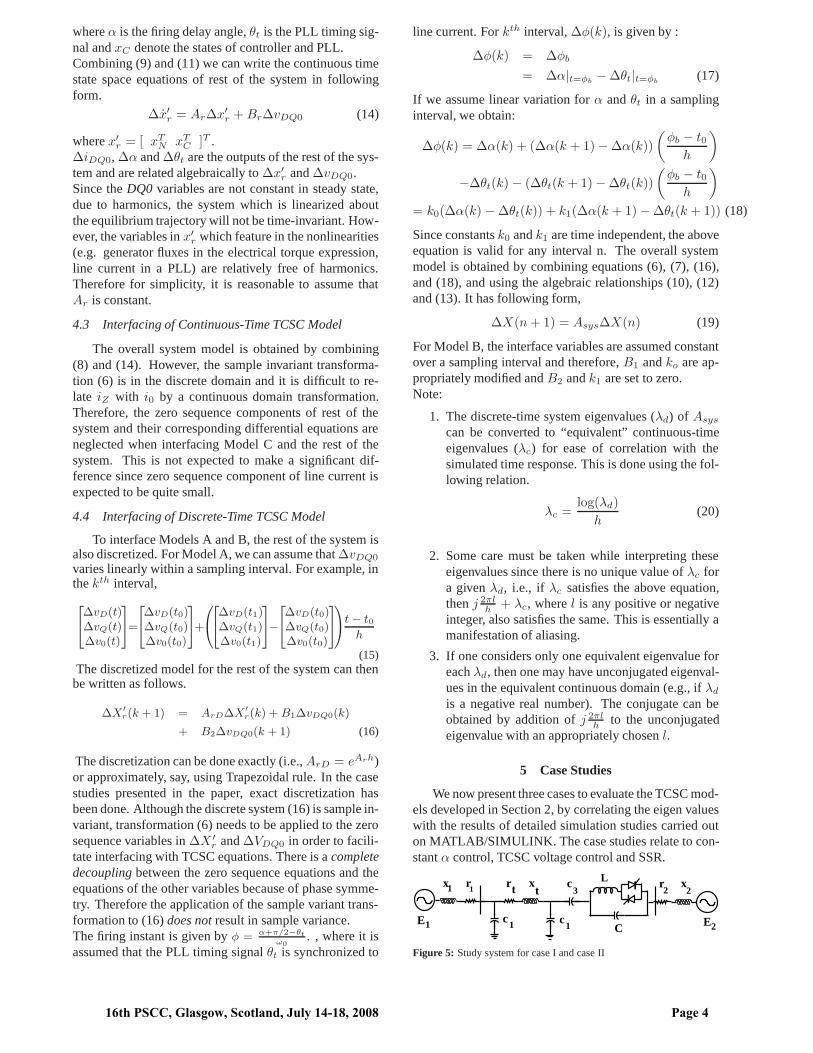
We now present three cases to evaluate the TCSC mod-els developed in Section 2, by correlating the eigen valueswith the results of detailed simulation studies carried outon MATLAB/SIMULINK. The case studies relate to con-stantα control, TCSC voltage control and SSR.

1L

C

r

E1 E2

2 2

c c

3

11

ttx1 r x c r x

Figure 5: Study system for case I and case II

16th PSCC, Glasgow, Scotland, July 14-18, 2008 Page 4

The test system for Case I and II consists of a 400 kV,400 km transmission line compensated by a fixed seriescapacitor along with TCSC and constant voltage sourcesat both ends of line. The single line diagram of the studysystem is shown in Fig 5. The system data, PLL data andPLL block diagram are given in Appendix A and B. Thefixed capacitor provides 27% compensation and TCSCprovides 8% in blocking mode. The transmission line isrepresented by aπ model.

5.1 Case I

Table 1: Eigenvalues atα0 = 155 ˚

Model A Model B Model CSr. No. Equivalent Continuous Domain Eigenvalues1 -2.43 ±j563.75 -38.13±j560.6

2 -2.76 ±j908.48 -0.72 ±j893.52 -2.82 ±j4683.3

3 -1.65 ±j621.55 -2.47 ±j622.02

4 -2.78 ±j280.12 3.65 ±j284.06 -2.64 ±j4055.1

5 -2.07 ±j71.44 -2.10 ±j71.22 -2.07 ±j3698.7

6 -2.11 ±j700.00 -3.41 ±j700.89 -2.06 ±j3070.4

7 -19.20±j459.74 -18.26±j472.19 -16.93 ±j458.68

8 -24.53±j164.28 -23.13±j169.00 -17.42 ±j165.99

9 -20.46±j864.24 -21.10±j864.47

10 -0.40 -0.40 -0.4011 -218.71 -207.06 -239.7512 -28.28±j629.95 1.91 ±j618.9 -28.63±j633.23

13 -29.33 -27.72 -30.84

Table 2: Eigenvalues atα0 = 165 ˚

Model A Model B Model CSr. No. Equivalent Continuous Domain Eigenvalues1 -2.50 ± j564.49 -14.13 ±j574.08

2 -2.78 ± j908.49 -0.51 ±j893.67 -2.27±j4696

3 -1.64 ± j621.53 -1.60 ±j621.52

4 -2.79 ± j280.10 3.60 ± j284.11 -5.66±j4065.9

5 -2.07 ± j71.44 -2.06 ±j71.31 -2.07±j3699.2

6 -2.11 ± j699.88 -3.01 ±j700.29 -2.21±j3070.8

7 -23.53± j472.62 -0.66 ±j475.88 -32.2±j476.7

8 -24.55± j145.98 -37.08±j152.9 -23.6±j145.2

9 -26.79± j862.03 -27.72±j859.65

10 -0.40 -0.40 -0.411 -293.47 -349.22 -279.812 -155.63±j305.82 -146.22±j250.38 -151.0±j318.14

13 -184.32+j942.48 -179.59+j942.48 -201.31+j942.79

The eigen-analysis presented in this sub-section is for afixedα. The TCSC model is tested for two different op-erating conditions,α0 = 165 ˚ and α0 = 155 ˚ . Theequivalent continuous time eigenvalues (λc) are shown inTable 1 and Table 2.The 12th and 13th modes correspond to the TCSC stateswhile 10thand11th modes correspond to PLL. The modes2,4,5,6,7,8 can be easily correlated to the modes of ModelC if j 2πl

his added to the eigenvalues, wherel is an integer.

The modes 1, 3 and 9 are mainly associated with the trans-formed zero sequence variables of the network. Thesemodes are not shown in results of eigen-analysis of thesystem with Model C (see discussion in Section 4.3). Themodes 7 and 8 are subsynchronous and super-synchronousnetwork modes of the system respectively, correspondingto series capacitive compensation.Model B indicates that one (atα0 = 155 ˚ ) or two(at α0 = 165 ˚ ) super-synchronous modes are unstable.Also, the damping of the super-synchronous mode corre-sponding to fixed series compensation (mode 7) is sub-stantially lower for Model B whenα0 = 165 ˚ . On the

other hand, Models A and C give similar results.We have carried out a detailed digital simulation of thesame system using a50 µs time step. The responses areobtained for two degree pulse change of firing delay angleand are given in Fig. 6 and Fig. 7.

0.5 0.6 0.7 0.8 0.9 1 1.1 1.2 1.3

−25

−20

VD

[ k

V ]

0.5 0.6 0.7 0.8 0.9 1 1.1 1.2 1.3−4

−2

0

2

VQ

[ k

V ]

0.5 0.6 0.7 0.8 0.9 1 1.1 1.2 1.3−5

0

5

Time [ Sec ]

V0

[ kV

]

Figure 6: Response of system for 2 ˚ pulse change inα atα0 = 155 ˚

0.5 0.6 0.7 0.8 0.9 1 1.1 1.2 1.3

−14.5

−14

−13.5

VD

[ k

V ]

0.5 0.6 0.7 0.8 0.9 1 1.1 1.2 1.3−1

−0.5

0

VQ

[ k

V ]

0.5 0.6 0.7 0.8 0.9 1 1.1 1.2 1.3

−0.5

0

0.5

Time [ Sec ]

V0

[ kV

]

Figure 7: Response of system for 2 ˚ pulse change inα atα0 = 165 ˚

Clearly, no instability is seen, indicating that Model Bdoes not give an accurate prediction of stability. More-over, the eigenvalue near−29 predicted by eigen-analysis(Model A and C) is clearly manifested as the dominantmode in Fig. 6. Forα0 = 165 ˚ , the damped oscillatorymode nearj145 rad/s is seen in the simulation result, -Fig. 7

5.2 Case II

A TCSC can be made to operate in reactance, volt-age, current or power control modes. To check the accu-racy of the models, we consider a controller which reg-ulates the magnitude of TCSC voltageVC , whereVC =√

v2D + v2

Q + v20 as shown in Fig. 8.

16th PSCC, Glasgow, Scotland, July 14-18, 2008 Page 5

−Σ

+− −

√

v2D + v2

Q + v20

KPC

KIC

s

Vref α

Figure 8: TCSC voltage regulator

In Table 3, the instability gains predicted by variousTCSC models are given along with the instability gain ob-tained from detailed digital simulation, for two operating

conditions. The ratioKIC

KPC

is maintained at 50.

Table 3: Instability Gain,KPC in Degrees/kV

Vref =14 kV Vref =24 kVInstability gain seen in detaileddigital simulation

8.50 (552.0 rad/s) 2.55 (610.0 rad/s)

Model A 11.20 (524.4 rad/s) 3.00 (606.7 rad/s)Model A (line shunt capacitanceneglected)

11.22 (526.5 rad/s) 2.95 (606.4 rad/s)

Model C 2.12 (4692.8 rad/s) 2.38 (613.3 rad/s)Model C (line shunt capacitanceneglected)

6.30 (516.8 rad/s) 2.35 (615.3 rad/s)

The instability gain predicted by Model A matches closelywith that seen in detailed digital simulation. When shuntcapacitance of the line is considered, a high frequencymode of frequency 4692.8 rad/s is shown to be unstablewhich does not manifest in the simulation. However, ifshunt capacitance of the line is neglected, the instabilitygain predicted by Model C matches closely with the sim-ulation.The simulated response of the system when gains areswitched from 0.9 to 1.2 times the instability gain areshown in Figs. 9 and 10. Note that frequency of the unsta-ble mode obtained by inspection of the time response (ap-proximately 88Hz forVref = 14 kV and 97 Hz forVref =24 kV) also matches closely with the prediction of ModelA.

Figure 9: Instability seen in simulated response -Vref = 14kV

Figure 10: Instability seen in simulated response -Vref = 24kV

5.3 Case III

We now present the analysis of IEEE First BenchMark (FBM) system [8] with the various TCSC models.A TCSC is included in series with the fixed series capac-itor. The parametersL andC of TCSC are such that its

natural frequency 1√LC

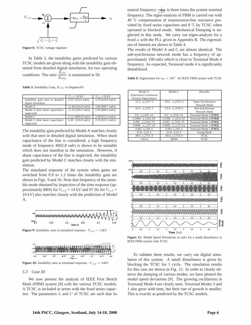
is three times the system nominalfrequency. The eigen-analysis of FBM is carried out with40 % compensation of transmission-line reactance pro-vided by fixed series capacitors and 8% by TCSC whenoperated in blocked mode. Mechanical Damping is ne-glected in this study. We carry out eigen-analysis for afixedα with the PLL given in Appendix B. The eigenval-ues of interest are shown in Table 4.The results of Model A and C are almost identical. Thesub-synchronous network mode has a frequency of ap-proximately 190 rad/s which is close to Torsional Mode 4frequency. As expected, Torsional mode 4 is significantlydestabilized.

Table 4: Eigenvalues forα0 = 160 ˚ for IEEE FBM system with TCSC

Model A Model C Remarks(Equivalent ContinuousDomain Eigenvalues)

-12.5 ±j557.5 -16.6 ±j555.5 Super-SynchronousNetwork Mode

-16.2 ±j191.1 -15.4 ±j190.5 Sub-SynchronousNetwork Mode

0.0 ±j298.18 0.0 ±j298.18 Torsional Mode 5(TM5)0.2696±j202.69 0.2596±j202.68 Torsional Mode 4(TM4)0.091 ±j160.72 0.091 ±j160.73 Torsional Mode 3(TM3)0.0096±j127.04 0.0093±j127.04 Torsional Mode 2(TM2)

0.067±j99.3 0.064±j99.3 Torsional Mode 1(TM1)-0.41±j9.5 -0.41±j9.5 Swing Mode

-89.5±j751.8 -85.6±j759.0 TCSC-101.4 -98.60 TCSC

0 0.5 1 1.5 2 2.5 3 3.5 4 4.5 5−0.01

0

0.01

TM

5

0 0.5 1 1.5 2 2.5 3 3.5 4 4.5 5−2

0

2

0 0.5 1 1.5 2 2.5 3 3.5 4 4.5 5−1

0

1

0 0.5 1 1.5 2 2.5 3 3.5 4 4.5 5−1

0

1

0 0.5 1 1.5 2 2.5 3 3.5 4 4.5 5−1

0

1

0 0.5 1 1.5 2 2.5 3 3.5 4 4.5 5

−1

0

1

Time [ s ]

TM

4T

M3

TM

2T

M1

Swin

gM

ode

Figure 11: Modal Speed Deviations in rad/s for a small disturbance inIEEE FBM system with TCSC

To validate these results, we carry out digital simu-lation of this system. A small disturbance is given byblocking the TCSC for 1 cycle. The simulation resultsfor this case are shown in Fig. 11. In order to clearly ob-serve the damping of various modes, we have plotted themodal speed deviations [9]. The growing oscillations inTorsional Mode 4 are clearly seen. Torsional Modes 3 and1 also grow with time, but their rate of growth is smaller.This is exactly as predicted by the TCSC models.

16th PSCC, Glasgow, Scotland, July 14-18, 2008 Page 6

6 Discussion

Model A was found to be consistently accurate in allthese cases, whereas Model B shows spurious instability.Although Model C involves additional approximations, itis convenient to use since it does not require discretizationof the rest of the system. Since most tools for controllerdesign and SSR analysis are formulated in the continuousdomain, Model C is a natural choice. While we did ob-serve spurious instability in Case II when using this model,it arose due to the presence of very high frequency dynam-ics. When shunt capacitances of the system were ignored,this model gave accurate results. For relatively slower dy-namics associated with sub-synchronous torsional modes,Model A and C gave almost identical results.Additional cases with different (1) firing angles (2) levelsof compensation (3) ratios of fixed and TCSC capacitivereactances, were also considered. These gave similar in-ferences as above.The controllers and PLL used in this paper are based onDQ variables; this results in relatively simple models.With individual (‘per phase’) firing and control schemes,there is an increase in modelling complexity and thederivations can become quite tedious. However, modu-larity is the redeeming virtue of these models, because thederivations can be done independent of the rest of the sys-tem and involve a one-time effort.

7 Conclusion

A comparative evaluation of variants of six-sampleper cycle, modular and sample-invariant models has beendone. The discrete-time model with linear variation of in-terface variables is found to give good accuracy under alltested situations, whereas maintaining interface variablesconstant in a sampling interval can give incorrect infor-mation of the stability of super-synchronous network orTCSC modes. Conversion of the TCSC model to continu-ous domain before interfacing to the network is convenientand is accurate in most cases.These linearized models have sufficient accuracy andbandwidth for design and parametric studies relating toSubsynchronous resonance, controller and low frequencynetwork and torsional modes. Modularity and sample-invariance ensure their easy implementation in computerprograms. They can be a useful complement to digitalsimulation studies and should find greater use in the fu-ture.

Acknowledgment

The financial support received under RSOP from Cen-tral Power Research Institute (CPRI), Ministry of Power,Government of India is gratefully acknowledged.

REFERENCES

[1] A. Ghosh and G. Ledwich,“Modelling and controlof thyristor controlled switched Compensators”,IEEProc. Genr. Transm. Disrib.,vol.142, no.3, pp. 297-304, May 1995.

[2] R. Rajaraman, Ian Dobson, R. H. Lasseter and Y. Sh-ern, “Computing the damping of subsynchronous os-cillations due to thyristor controlled switched capac-

itor”, IEEE Trans. on Power Delivery., vol.11, no.2,pp. 1120-1127, April 1996.

[3] Sasan G. Jalali, Robert H. Lasseter and Ian Dob-son, “Dynamic Response of a Thyristor ControlledSwitched Capacitor”,IEEE Trans. on Power Deliv-ery, vol.9, no.3, pp. 1609-1615, July 1994.

[4] Sasan G. Jalali, R A Hedin, M. Pereira and K. Sadek,“A stability model for the advanced series com-pensator (ASC)”, IEEE Trans. on Power Delivery,vol.11, no.2, pp. 1128-1137, Apr 1996.

[5] Hisham A. Othman and Lennart Angquist, “Analyti-cal Modelling of Thyristor-Controlled Series Capac-itor For SSR Study”, IEEE Trans. on Power Syst,vol.11, no.1, pp. 119-127, Feb 1996.

[6] Khosro Kabiri, Sebastian Henschel, Jose RamonMartı and Hermann W. Dommel, “A Discrete State-Space Model for SSR Stabilizing Controller Designfor TCSC Compensated System”,IEEE Trans. onPower Delivery, vol.20,, no. 1, pp. 466-473, Jan2005.

[7] Lennart Angquist, “Synchronous voltage ReversalControl of Thyristor Controlled Capacitor” , PhDThesis, Royal Institute of Technology, Stockholm,2002.

[8] IEEE Subsynchronous Resonance Task Force, FirstBench Mark Model for Computer Simulation of Sub-synchronous Resonance,IEEE Trans. Power Appa-ratus and Systems, Vol. PAS-96, no. 5, pp. 1565-1572, Sep./Oct. 1977.

[9] K. R. Padiyar, Analysis of Subsynchronous Reso-nance in Power Systems., 1st ed, USA: Kluwer Aca-demic Publishers, 1999.

A System Data for Case I and II

Transmission Line ω0 = 314.159 rads

PositiveSequence

rt xt B1

11.9168 Ω 132.8 Ω 6.9375 × 10−4

ZeroSequence

r0 x0 B0

64.768 Ω 496 Ω 4.48 × 10−4

Voltage SourcesE1 r1 + jx1 E2 r2 + jx2

400∠20 ˚ kV 0.1 +j13.5088 Ω 400∠0 ˚ kV 0.1 +j8.1681 Ω

Series Compensation PLLL C c3 KP Ki

4.4mH 306µF 90µF 144.34rads

57.74 rads2

B PLL Block Diagram

Oscillatore

e

︷ ︸︸ ︷

θt = ω

θt

ω0

ω

0 1√3

2−1

2

−√

3

2−1

2

sin

cos

U1

PI

U2

iaI

+

+Σ

Controlled

U2

0 1 −1

−1 0 1

1 −1 0

U′1

ibI

icI

∝sin(ω0t+tan−1 iDiQ− θt)I =

√

i2a + i2b + i2c

Figure 12: PLL

16th PSCC, Glasgow, Scotland, July 14-18, 2008 Page 7