comparative analysis of empirical descriptions of
TRANSCRIPT

Powder Technology 270 (2015) 393–410
Contents lists available at ScienceDirect
Powder Technology
j ourna l homepage: www.e lsev ie r .com/ locate /powtec
Comparative analysis of empirical descriptions of eccentric flow in silomodel by the linear and nonlinear regressions
Irena Sielamowicz a,⁎, Artur Czech b, Tomasz A. Kowalewski c
a University of Zielona Góra, 65-516 Zielona Góra, Prof. Z. Szafrana 1, Polandb Bialystok University of Technology, Wiejska 45 A, Bialystok, Polandc Institute of Fundamental Technological Research, Polish Academy of Sciences, Pawińskiego 5B, Warsaw, Poland
⁎ Corresponding author.E-mail addresses: [email protected] (I. Sie
(A. Czech), [email protected] (T.A. Kowalewski).
http://dx.doi.org/10.1016/j.powtec.2014.10.0070032-5910/© 2014 Elsevier B.V. All rights reserved.
a b s t r a c t
a r t i c l e i n f oArticle history:Received 9 June 2014Received in revised form 29 September 2014Accepted 3 October 2014Available online 14 October 2014
Keywords:Eccentric granular flowSilo modelEmpirical descriptionLinear and nonlinear regressionGaussian descriptionDouble logarithm
This paper is a third of a series of the threewhere eccentric cases of flow in silomodels recorded by theDPIV tech-nique are presented and discussed in detail. The methodology of empirical descriptions of velocities, flow rateand stagnant zone boundaries on the base of registered velocity fields in eccentric filling and discharge in 2Dsilo model was discussed. In previous two papers [1,2] we analyzed also eccentric flows but with different loca-tions of the outlet. It was stated that in practice even tiny eccentricity of filling or discharge processesmay lead toquite an unexpected behavior of the silo structure. During asymmetrical processes, flow patterns andwall stress-es may be quite different. It is therefore crucial to identify how flow patterns developed in the material duringeccentric filling or discharge and to determine both the flow rate and wall stresses occurring under such stateof loads. Thus,we discuss here the third case of discharge— located in the center of the silo bottom. A comparisonof these three cases of discharge mode will be presented in the next paper. Empirical descriptions of eccentricflow velocities in silo model by the linear and nonlinear regressions are presented here with specific functionslike the Gaussian function and “the double logarithmic function”. In both methods the velocity was alsodescripted by linearization and in the Gaussian method also by the nonlinear method of Gauss–Newton and inthe case of the method of double logarithm — the nonlinear method of Levenberg–Marquardt was applied.Velocities were predicted by using interpolation due to the nonlinear model of the Gaussian type and to thenonlinear function of “the double logarithm”.
© 2014 Elsevier B.V. All rights reserved.
1. Literature review
Eccentricity is always a dangerous factor influencing to the silostructure. Technological processes canbe disruptedwhile any eccentric-ity occurred. International Standards usually relate to axial symmetricstates of stresses and even avoid defining discharge pressures andflow patterns because of continuing uncertainties defining the flowchannel geometry and wall pressures under eccentric discharge or thevalues of increased coefficients of horizontal pressure during eccentricdischarge [3,4]. In [3–6] we read comments on the eccentricity of theoutlet, on the flow channel geometry and the wall pressure under ec-centric discharge. Eccentric discharge is described as a flow pattern inthe stored solid arising frommoving solid being asymmetrically distrib-uted relative to the vertical centreline of the silo. This normally arises asa result of an eccentrically located outlet but can be caused by otherasymmetrical phenomena which are not clearly defined. As it wascommented in [1] calculations for flow channel geometry are requiredfor only one size of flow channel contact with the wall, which should
lamowicz), [email protected]
be determined for ΘC = 35° and wall pressures under eccentric dis-charge are also defined and discussed in [1]. Researchers tried to makeapproaches to develop designing of bins under eccentric discharge[7–9] and Carson [10] in detail presented the issue of eccentricity asone of the major causes of hopper failures. Eccentricity of the flow tothe silo axis causes the pressure patterns to become much morecomplex than in centric cases. In the field of silo investigations threemain issues are usually analyzed: pressures under eccentric discharge,flow patterns and stagnant zone boundaries.
Works on eccentric discharge have been published for many yearsand a few researchers have dealt with this complicated problem. In [1]one canfind a detail discussion of investigations in silos during eccentricdischarge, silo loads and wall loads, measurements of wall loads whenunloaded eccentrically, the effect of eccentric unloading in a model binfor different unloading rates, the effect of eccentricity and ways of dis-charge in silo, flow patterns in a silo with symmetrical and eccentricoutlet. There are works [7–13] where authors investigated the behaviorof silos under eccentric discharge, identified flow patterns and stresseson the wall during centric and eccentric discharges. They also mademeasurements of the wall pressures under eccentric discharge, investi-gated discharge and the eccentricity of the hopper influence on silo wallpressures, and measured experimentally the heights of the stagnant

394 I. Sielamowicz et al. / Powder Technology 270 (2015) 393–410
zones for two kinds of granular materials after hopper eccentric andcentric discharges. Theoretical analyses were made using the kinematicmodel, proposed by Nedderman and Tüzün [10,13,14], for filling anddischarge — centrally and eccentrically. Further numerical investiga-tions were conducted in [15,16] by applying FEMmodeling in the anal-ysis of influence of hopper eccentricity on wall pressures or a bucklingstrength of steel silo subject to code specified pressures for eccentricdischarge. Another field of investigationswas related to localized defor-mation pattern in granularmaterials, investigating shear localizations ingranular materials numerically and compared the obtained results toexperimental data [17]. In [18] one can find a long list of referencesconcerning investigation of eccentric discharge.
Investigation of flow patterns and wall stresses in silos and otherhoppers is usually carried out on laboratory models. Many differentmeasurement techniques have been used in such studies: visual mea-surements through transparent walls, colored layers and photography,colored layers and dissection after freezing the flow with paraffin wax,photographic or video techniques, and tracer techniques using X-raysand radio pills and insertion of markers to measure residence times[18]. In laboratory tests very significant scale effects in silo flow andpressures were reported in [19–23]. However, almost all of these tech-niques are not viable at full scale. Many tests on full scale silos weremade to measure wall pressures [24]. There are a few examples givenin literature where themeasurements of flow patterns were performedon line [18,25,26]. Such investigations are very expensive, due not onlyto the enormous size of the silo but also to the difficulties in accessingthe structure. Because of the difficulties of access at natural scale suchas opaque walls, opaque solids, surface covered with dust and intrusiveinvestigation techniques, such as the penetration of the wall, rarelyacceptable by silo owners, model silo studies seem to be very useful inthe recognizing flow patterns. Though, the challenge of observing flowprocesses at full scale remains considerable. The flow inside the silohas been poorly identified till today and the investigation of flowmodes inside the silo is almost impossible.
Silos are structures having round horizontal cross sections. Usuallyall laboratory models are flat and only flat flow is investigated. Thereare also round laboratory models but in this case, it is much moredifficult to measure stagnant zone boundaries. In such models usuallythe problem of flow modes and determining wall pressures are made.
2. Experimental procedure
To register velocities of flowing grains we applied the DPIV (DigitalParticle Image Velocimetry) technique which made it possible toidentify the eccentric flow in the plane flat-bottomed model silo madeof Plexiglas. Two other eccentric cases of the flow were discussed in[1,2]. The images of the flowing material were recorded by a high-resolution camera and evaluated using theDPIV technique. The adoptedDPIV technique was based on the optical flow algorithm, which hasbeen found to be most reliable for granular flow images. In [43] theauthors presented a detailed description of the OF-DPIV, including itsdevelopment and application. The experimental setup used for theflow analysis consisted of a transparent acrylic plastic box, a set ofillumination lamps, and a high-speed CCD camera (PCO1200HS) withan objective 50 mm lens produced by PCO AG, Kelheim, Germany[http://www.pco.de/high-speed-cameras/pco1200-hs/]. The transpar-ent flat-bottom silo model had a height 800 mm, a depth of 100 mmand a width of 260 mm. The model was placed on a stand and granularmaterial was supplied through a box suspended above the model. Thebottom of the supplying box contained a sieve and the box was filledwith flax seeds to 2/3 of its height. The model was filled close to theleft wall. The discharge outlet was located centrally at the bottom ofthe silo. The width of the outlet was 10 mm. In order to evaluatetransient velocity fields, long sequences of 100–400 images weretaken at variable time intervals, covering the whole of the dischargetime. The DPIV technique used here produced velocity fields for the
full interrogation area. The velocity profiles obtained inside the quasitwo-dimensional silo were smooth and free of shock-like discontinu-ities. The flax seeds showed some effects of static electricity whenflowing and sliding over the transparent acrylic plastic. The granularmaterial was introduced in a form of a uniform stream into the silomodel to obtain uniform and repeatable packing of the material withno particle segregation. The evolution of the flow region and the tracesof flowing particles were evaluated from recorded images. Pairs of dig-ital short exposure images were taken to describe how the velocity fieldvaries in the flowing material. This data was used in empirical descrip-tion of the flow. The properties of the amaranth seed used in the exper-iments were: wall friction against transparent Plexiglas φw=26°, angleof internal friction φe = 25° granular material density depositedthrough a pipe with zero free-fall 746 kg/m3 at 1 kPa and 747 kg/m3
at 8 kPa, Young's modulus 6.11 MPa. The values of the angle of in-ternal friction for the flax-seed are taken from the Polish StandardPN-89/B-03262. Sequences of 12-bit images with the resolution of1280 × 1024 pixels were acquired by Pentium 4 based personal com-puter using IEEE1394 interface. The system allowed acquiring up to1000 images at time interval of 1.5 ms (667 fps). The velocity fieldwas evaluated for triplets of images using the DPIV based on the OpticalFlow technique. Dense velocity fields with vectors for each pixel of theimage were obtained and used for further evaluation of the velocityprofiles, velocity contours and streamlines. The term “streamline” is de-fined as a direction of theflow of different particles at the same time. In-trinsic resolution of the PIV technique is limited by the size of the area ofinterest that is used in the application of the cross correlation algorithmbetween subsequent images and this is generally one order of magni-tude larger than a single pixel. The aim of the present investigation isto explore the possibility of using the Optical Flow technique based onPIV in measuring granular material flow velocity. In granular materialflowoneusually visualizes a track of individual particles, not necessarilycoinciding with the streamline. Such tracks were obtained by Choi et al.[11], who used a high-speed imaging technique to trace the position ofsingle particles in granular materials. Velocity profiles obtained thatway for the flow of granular material inside a quasi-two-bottomedsilo were smooth and free of shock-like discontinuities. In contrast,theDPIV technique used here produces velocityfield for the full interro-gation area, and this can be used to predict the natural track ofindividual particles.
In general, this techniquewas applied in fluidmechanics and its firstapplications to granularmaterial flowwere presented by [27,28]. One ofthe first successful attempts to apply the PIV technique to granularmatter was described in [28–35] and reported the use of the PIV tech-nique in their experiments to obtain information on local velocities ofparticles at several elevations in densely packed materials. Ostendorfand Schwedes in [30] combined PIV measurements with wall normalstress measurements at different points of time in a large scale silo.
Observations of the discharge process allow us to understand thebehavior of theflowingmaterial. Asmentioned above, differentmeasure-ment techniques havebeenused in investigations offlow in silomodels. Anumber of experimental works have been focused to measure flow pat-terns. Optical techniques are commonly used in the analysis of velocityprofiles near the transparent silo walls. The X-ray technique was fre-quently applied to obtain information from deeper flow layers [36,37].Also, other non-invasive measurement techniques were applied to regis-ter granular flow, density and velocity fields in flowing zones, amongothers spy-holes, radio transmitters, positron emission [38],magnetic res-onance imaging, radioactive tracers, and ultrasonic speckle velocimetry.More details on different techniques used in investigations of granularflow in small models can be found in references given in [28,38–42].
The case discussed here is recognized as eccentric filling but the po-sition of the outlet that was symmetrically located was shown in Fig. 1.This location of the outlet produces a very interesting flowmode of thematerial, becoming symmetrical very quickly after opening the outlet.Despite eccentric feeding, just after 25th of the flow, the material
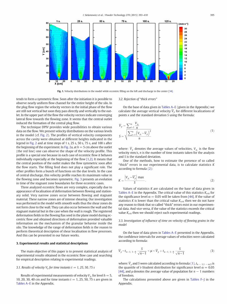
Fig. 1. Velocity distributions in the model while eccentric filling on the left and discharge in the center [34].
395I. Sielamowicz et al. / Powder Technology 270 (2015) 393–410
tends to form a symmetric flow. Soon after the initiation it is possible toobserve nearly uniform flow channel for the entire height of the silo. Inthe plug flow region the velocity vectors in the initial phase of the floware still not vertical but soon they pass directly and vertically to the out-let. In the upper part of theflow the velocity vectors indicate converginglateral flow towards the flowing zone. It seems that the central outletinduced the formation of the central plug flow.
The technique DPIV provides wide possibilities to obtain variousdata on the flow.We present velocity distributions on the various levelsin the model (cf. Fig. 2). The profiles of vertical velocity componentsacross the cavity were obtained at different heights indicated in thelegend in Fig. 2 and at time steps of 1 s, 25 s, 50 s, 75 s, and 100 s afterthe beginning of the experiment. In Fig. 2a, at h=5 cmabove the outlet(the red line) one can observe the shape of the velocity profile. Thisprofile is a special one because in each case of eccentric flow it behavesindividually especially at the beginning of the flow [1,2]. It means thatthe central position of the outlet makes the flow symmetric soon afterthe flow starts. The filling feed does not play a significant role. Theother profiles form a bunch of functions on the due levels. In the caseof central discharge, this velocity profile reaches its maximum value inthe flowing zone and becomes symmetric. Fig. 3 presents an evolutionin time of the stagnant zone boundaries for three eccentric cases.
Three analyzed eccentric flows are very complex, especially due toappearance of localisation of deformation between flowing and station-ary solid. Very narrow zones occur between flowing and stagnantmaterial. These narrow zones are of intense shearing. Our investigationwas performed in themodel with smoothwalls thus the shear zones donot form close to thewall. They can also occur between thewall and thestagnantmaterial but in the casewhen the wall is rough. The registereddeformationfields in the flowingflax seed in the planemodel during ec-centric flow and obtained directions of deformation provided valuableinformation on the mechanism of the granular behavior inside thesilo. The knowledge of the range of deformation fields is the reason toperform theoretical description of shear localisation in flow processes.And this can be presented in our future works.
3. Experimental results and statistical descriptions
The main objective of this paper is to present statistical analysis ofexperimental results obtained in the eccentric flow case and searchingfor empirical description relating to experimental readings.
3.1. Results of velocity Vy for time instants t = 1, 25, 50, 75 s
Results of experimental measurements of velocityVyi for level h=5,10, 20, 30, 40 cm and for time instants t = 1, 25, 50, 75 s are given inTables A–E in the Appendix.
3.2. Rejection of “thick errors”
On the base of data given in Tables A–E (given in the Appendix) wecalculate the average vertical velocity Vy for different localizations ofpoints x and the standard deviation S using the formula:
Vy ¼Xn
i¼1
Vyi
n
S ¼
ffiffiffiffiffiffiffiffiffiffiffiffiffiffiffiffiffiffiffiffiffiffiffiffiffiffiffiffiffiffiffiffiffiffiffiffiffiXni¼1
Vyi−Vy
� �2
n
vuut ð1Þ
where: Vy denotes the average values of velocities, Vyiis the flow
velocity mm/s, n is the number of time instants taken for the analysisand S is the standard deviation.
One of the methods, how to estimate the presence of so called“thick” errors in our experimental data, is to calculate statistics Kaccording to formula (2):
K ¼Vyi
−Vy
������ max
S: ð2Þ
Values of statistics K are calculated on the base of data given inTables A–E in the Appendix. The critical value of this statistics Kcrit forthe significance level α = 0.05 will be taken from [44]. If the value ofstatistics K is lower than the critical value Kcrit then we do not haveany reason to think that so called “thick” errors exist in our experimen-tal data. And vice versa, if the value of the statistics exceeds the criticalvalue Kcrit then we should reject such experimental readings.
3.3. Investigation of influence of time on velocity of flowing grains in themodel
On the base of data given in Tables A–E presented in the Appendix,the confidence intervals for average values of velocities were calculatedaccording to formula:
Vy−tn−1; 1−α2
Sffiffiffiffiffiffiffiffiffiffiffin−1
p b μ b Vy þ tn−1; 1−α2
Sffiffiffiffiffiffiffiffiffiffiffin−1
p ð3Þ
where:Vy and Swere calculated according to formula (1), tn − 1,1 − α/2 isthe quantile of t-Student distribution for significance level α = 0.05[44], and μ denotes the average value of population for n − 1 numbersof freedom.
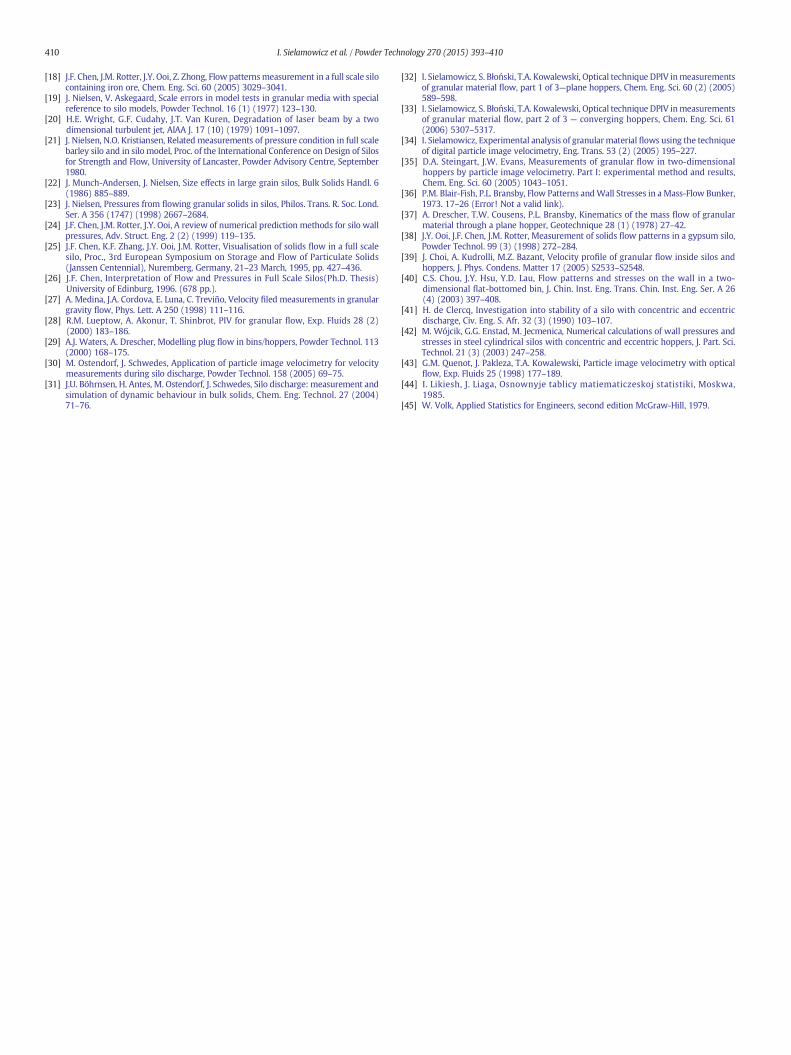
The calculations presented above are given in Tables F–J in theAppendix.

396 I. Sielamowicz et al. / Powder Technology 270 (2015) 393–410
Comparing data given in Tables A–E with data given in Tables F–Jpresented in the Appendixwe can state, that there is no reason to reject“zero hypothesis”, that means that time is not an important factorinfluencing on the velocity for any given point x.
3.4. Investigation of velocity values for points located symmetrical to thesilo symmetry axis
The axis of symmetry of the silo model is located in the distance atx = 13 cm from the lateral edge of the model. Symmetrical locationsof points are for abscissa 13− ni and 13+ ni, where ni is the readingsof velocities for points located on both sides of the axis of symmetryof the silo model.
We assume “the zero hypothesis” (H) and “the opposite hypothesis”(H1):
H : μ13−ni¼ μ13þni
; H1 : μ13−ni≠ μ13þni
and in this way we verify the hypothesis of the average value of twopopulations. To do this we calculate statistics t in the case of the same
Fig. 2.A–E) Velocity profiles for theflow offlax-seed obtained for A) eccentric filling on the left aG–J) velocity profiles on selected levels inside the model [34].
number of repetitions:
t ¼X13−ni
− X13þni
������ffiffiffiffiffiffiffiffiffiffiffiffiffiffiffiffiffiffiffiffiffiffiffiffiffiffiffiffiffiffiffi
S213−niþ S213þni
q ffiffiffiffiffiffiffiffiffiffiffin−1
pð4Þ
or in the case of different numbers of repetitions of experiments byformula (5):
t ¼X13−ni
−X13þni
������ffiffiffiffiffiffiffiffiffiffiffiffiffiffiffiffiffiffiffiffiffiffiffiffiffiffiffiffiffiffiffiffiffiffiffiffiffiffiffiffiffiffiffiffiffiffiffiffiffiffiffiffiffiffiffiffi
n13−niS213−ni
þ n13þniS213þni
qffiffiffiffiffiffiffiffiffiffiffiffiffiffiffiffiffiffiffiffiffiffiffiffiffiffiffiffiffiffiffiffiffiffiffiffiffiffiffiffiffiffiffiffiffiffiffiffiffiffiffiffiffiffiffiffiffiffiffiffiffiffiffiffiffiffiffiffiffiffiffiffin13−ni
n13þnin13−ni
þ n13þni−2
� �n13−ni
þ n13þni
vuut:
ð5Þ
The critical value in this case at the level of significance α = 0.05according to the t-Student is tcritical ¼ t0:05;13−ni ;13þni
.In this case when the value of statistics calculated from formula (4) to
(5) is higher than the critical value then the hypothesis H should berejected, in the opposite case there is no reason to reject the hypothesis.
Before calculating formulas (4) and (5), we have found the homoge-neity of the variance for various heights h in the model using the
nd discharge in the central part of the bottom; F) variation of velocity–distribution in time,
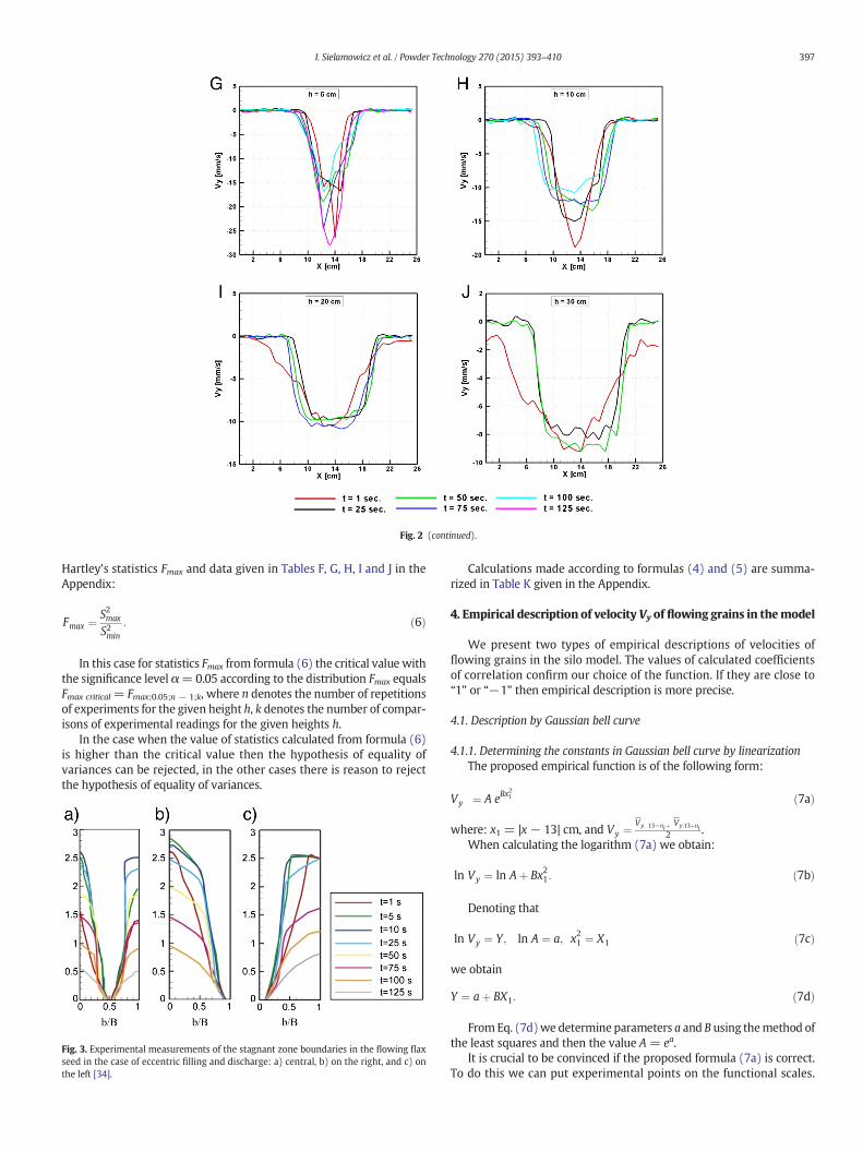
Fig. 2 (continued).
397I. Sielamowicz et al. / Powder Technology 270 (2015) 393–410
Hartley's statistics Fmax and data given in Tables F, G, H, I and J in theAppendix:
Fmax ¼S2max
S2min
: ð6Þ
In this case for statistics Fmax from formula (6) the critical value withthe significance level α=0.05 according to the distribution Fmax equalsFmax critical = Fmax;0.05;n − 1;k, where n denotes the number of repetitionsof experiments for the given height h, k denotes the number of compar-isons of experimental readings for the given heights h.
In the case when the value of statistics calculated from formula (6)is higher than the critical value then the hypothesis of equality ofvariances can be rejected, in the other cases there is reason to rejectthe hypothesis of equality of variances.
Fig. 3. Experimental measurements of the stagnant zone boundaries in the flowing flaxseed in the case of eccentric filling and discharge: a) central, b) on the right, and c) onthe left [34].
Calculations made according to formulas (4) and (5) are summa-rized in Table K given in the Appendix.
4. Empirical description of velocityVy of flowing grains in themodel
We present two types of empirical descriptions of velocities offlowing grains in the silo model. The values of calculated coefficientsof correlation confirm our choice of the function. If they are close to“1” or “−1” then empirical description is more precise.
4.1. Description by Gaussian bell curve
4.1.1. Determining the constants in Gaussian bell curve by linearizationThe proposed empirical function is of the following form:
Vy ¼ A eBx21 ð7aÞ
where: x1 = |x − 13| cm, and Vy ¼Vy; 13−niþ Vy;13þni
2 .When calculating the logarithm (7a) we obtain:
ln Vy ¼ ln Aþ Bx21: ð7bÞ
Denoting that
ln Vy ¼ Y ; ln A ¼ a; x21 ¼ X1 ð7cÞ
we obtain
Y ¼ aþ BX1: ð7dÞ
FromEq. (7d)we determine parameters a and B using themethod ofthe least squares and then the value A = ea.
It is crucial to be convinced if the proposed formula (7a) is correct.To do this we can put experimental points on the functional scales.
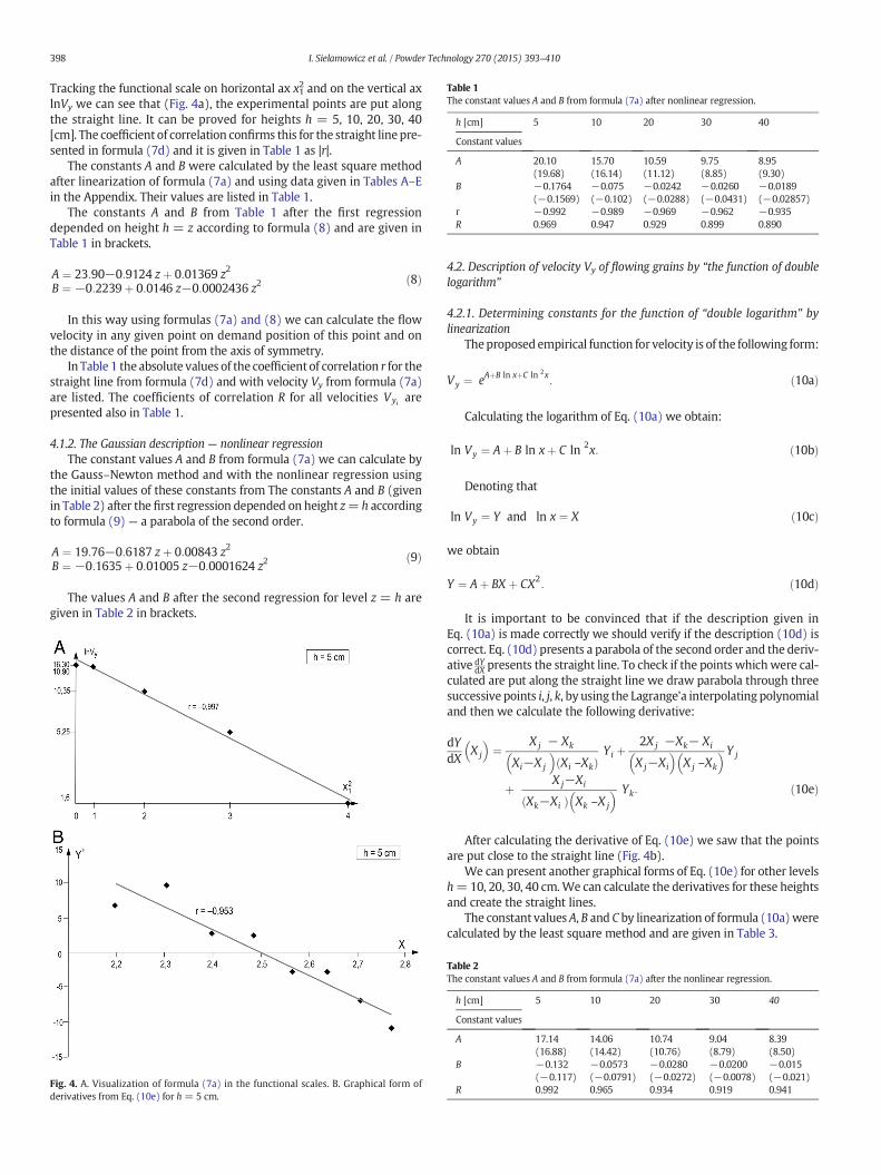
Table 1The constant values A and B from formula (7a) after nonlinear regression.
h [cm] 5 10 20 30 40
Constant values
A 20.10(19.68)
15.70(16.14)
10.59(11.12)
9.75(8.85)
8.95(9.30)
B −0.1764(−0.1569)
−0.075(−0.102)
−0.0242(−0.0288)
−0.0260(−0.0431)
−0.0189(−0.02857)
r −0.992 −0.989 −0.969 −0.962 −0.935R 0.969 0.947 0.929 0.899 0.890
398 I. Sielamowicz et al. / Powder Technology 270 (2015) 393–410
Tracking the functional scale on horizontal ax x12 and on the vertical ax
lnVy we can see that (Fig. 4a), the experimental points are put alongthe straight line. It can be proved for heights h = 5, 10, 20, 30, 40[cm]. The coefficient of correlation confirms this for the straight line pre-sented in formula (7d) and it is given in Table 1 as |r|.
The constants A and B were calculated by the least square methodafter linearization of formula (7a) and using data given in Tables A–Ein the Appendix. Their values are listed in Table 1.
The constants A and B from Table 1 after the first regressiondepended on height h = z according to formula (8) and are given inTable 1 in brackets.
A ¼ 23:90−0:9124 zþ 0:01369 z2
B ¼ −0:2239þ 0:0146 z−0:0002436 z2ð8Þ
In this way using formulas (7a) and (8) we can calculate the flowvelocity in any given point on demand position of this point and onthe distance of the point from the axis of symmetry.
In Table 1 the absolute values of the coefficient of correlation r for thestraight line from formula (7d) and with velocity Vy from formula (7a)are listed. The coefficients of correlation R for all velocities Vyi arepresented also in Table 1.
4.1.2. The Gaussian description — nonlinear regressionThe constant values A and B from formula (7a) we can calculate by
the Gauss–Newton method and with the nonlinear regression usingthe initial values of these constants from The constants A and B (givenin Table 2) after the first regression depended on height z= h accordingto formula (9) — a parabola of the second order.
A ¼ 19:76−0:6187 zþ 0:00843 z2
B ¼ −0:1635þ 0:01005 z−0:0001624 z2ð9Þ
The values A and B after the second regression for level z = h aregiven in Table 2 in brackets.
Fig. 4. A. Visualization of formula (7a) in the functional scales. B. Graphical form ofderivatives from Eq. (10e) for h = 5 cm.
4.2. Description of velocity Vy of flowing grains by “the function of doublelogarithm”
4.2.1. Determining constants for the function of “double logarithm” bylinearization
Theproposed empirical function for velocity is of the following form:
Vy ¼ eAþB ln xþC ln 2x: ð10aÞ
Calculating the logarithm of Eq. (10a) we obtain:
ln Vy ¼ Aþ B ln xþ C ln 2x: ð10bÞ
Denoting that
ln Vy ¼ Y and ln x ¼ X ð10cÞ
we obtain
Y ¼ Aþ BX þ CX2: ð10dÞ
It is important to be convinced that if the description given inEq. (10a) is made correctly we should verify if the description (10d) iscorrect. Eq. (10d) presents a parabola of the second order and the deriv-ative dY
dX presents the straight line. To check if the points whichwere cal-culated are put along the straight line we draw parabola through threesuccessive points i, j, k, by using the Lagrange'a interpolating polynomialand then we calculate the following derivative:
dYdX
X j
� �¼ X j − Xk
Xi−X j
� �Xi –Xkð Þ
Yi þ2X j −Xk− Xi
X j−Xi
� �X j –Xk
� �Y j
þ X j−Xi
Xk−Xið Þ Xk –X j
� � Yk: ð10eÞ
After calculating the derivative of Eq. (10e) we saw that the pointsare put close to the straight line (Fig. 4b).
We can present another graphical forms of Eq. (10e) for other levelsh=10, 20, 30, 40 cm.We can calculate the derivatives for these heightsand create the straight lines.
The constant values A, B and C by linearization of formula (10a)werecalculated by the least square method and are given in Table 3.
Table 2The constant values A and B from formula (7a) after the nonlinear regression.
h [cm] 5 10 20 30 40
Constant values
A 17.14(16.88)
14.06(14.42)
10.74(10.76)
9.04(8.79)
8.39(8.50)
B −0.132(−0.117)
−0.0573(−0.0791)
−0.0280(−0.0272)
−0.0200(−0.0078)
−0.015(−0.021)
R 0.992 0.965 0.934 0.919 0.941

Fig. 5. Experimental results of velocities Vy and their empirical descriptions on levelh = 5 cm.
Table 3The constant values from formula (10a) calculated by using the linear regression.
h [cm] 5 10 20 30 40
Constant values
A −136.37(−141.84)
−81.53(−70.36)
−41.84(−34.61)
−15.47(−22.70)
−11.05(−16.74)
B 109.71(114.29)
67.34(57.90)
35.38(29.71)
14.41(20.31)
10.97(15.61)
C −21.62(−22.55)
−13.44(−11.49)
−7.05(−5.96)
−2.94(−4.12)
−2.28(−3.20)
R 0.983 0.873 0.805 0.920 0.889
399I. Sielamowicz et al. / Powder Technology 270 (2015) 393–410
The constant values A, B and C given in Table 3 depended onheight z = h according to formula (11):
A ¼ 1:130−714:881z; r ¼ −0:987
B ¼ 1:513þ 563:861z; r ¼ 0:985
C ¼ −0:434−110:601z; r ¼ −0:985:
ð11Þ
The values calculated from formula (11) are given in Table 3 inbrackets.
4.2.2. Description of velocity Vy using the nonlinear regressionThe constant values A, B and C from formula (10a) we can calculate
by the Levenberg–Marquardtmethod andwith thenonlinear regressionusing the initial values of these constants given in Table 3. Their valuesafter the nonlinear regression are presented in Table 4.
The constant values A, B and C given in Table 4 depended onheight z = h according to formula (12).
A ¼ 10:696−756:661z; r ¼ −0:998
B ¼ −5:906þ 593:511z; r ¼ 0:998
C ¼ 1:089−115:771z; r ¼ −0:988:
ð12Þ
The values of these parameters calculated for z= h after the secondregression are listed in Table 4 in brackets.
5. Analysis of empirical results
5.1. Comparison of empirical description with experimental results
In Figs. 5, 7, 9, 11, and 13 the comparison of experimental resultswith empirical description by the function of Gaussian type accordingto formula (7a) and using data given in Tables 1 and 2 is presented.
In Figs. 6, 8, 10, 12, and 14 the results of empirical description byfunction of “the double logarithm” according formula (10a) using thedata from Tables 3 and 4 are presented.
In Figs. 5–14 the constant values for the empirical description weredetermined by the method of linearization (linear regression is denotedas solid lines) and by the method of nonlinear regression (dotted lines).
Table 4Constant values for formula (10a) calculated by using the nonlinear regression.
h [cm] 5 10 20 30 40
Constant values
A −143.62(−141.24)
−59.46(−65.67)
−28.76(−27.74)
−16.98(−15.23)
−9.67(−8.82)
B 114.63(112.80)
48.74(53.45)
24.59(23.76)
15.25(13.88)
9.61(8.93)
C −22.43(−22.07)
−9.56(−10.49)
−4.85(−4.70)
−3.03(−2.77)
−1.96(−1.81)
R 0.994 0.968 0.918 0.928 0.920
In these figures we can see a good agreement of both descriptionsbut the better compatibility to the experimental results was obtainedby using the nonlinear regression. In Figs. 5, 7, 9, 11, and 13 the compar-ison between experimental results and the empirical description(Gaussian function) according to formula (7a) with data given inTables 1 and 2 is presented. In Figs. 4, 6, 8, 10, and 12 the comparisonbetween the experimental results and the empirical description (“thedouble logarithm” function) according to formula (10a) with usingdata given in Tables 3 and 4 is presented.
Analyzing Figs. 5–14 we can notice differences in empirical descrip-tions when determining the constant values in functions calculated bythe method of linearization (formulas 7a or 10a) and also in the caseof using the nonlinear regression. The better description was obtainedusing the nonlinear regression (the dotted lines in Figs. 5–14). Whencomparing the results,we can see that a special large discrepancy in em-pirical descriptions occurred in description for lower levels (h = 5, 10,20 cm). There are also differences both in the Gaussian descriptionand in the function of “the double logarithm”. In the first casewe obtain-ed symmetrical description relative to the symmetry axis of silo model,i.e. to the location of points at x=13 cm, in the other cases, the descrip-tion is not symmetrical due to the shape of the empirical function. Theseconclusions are also supported by the sum of the squares of differences
∑ Vyi exp−Vyi emp
� �2that is presented in Table 5a.
Fig. 6. Experimental results of velocities Vy and their empirical descriptions on levelh = 5 cm.
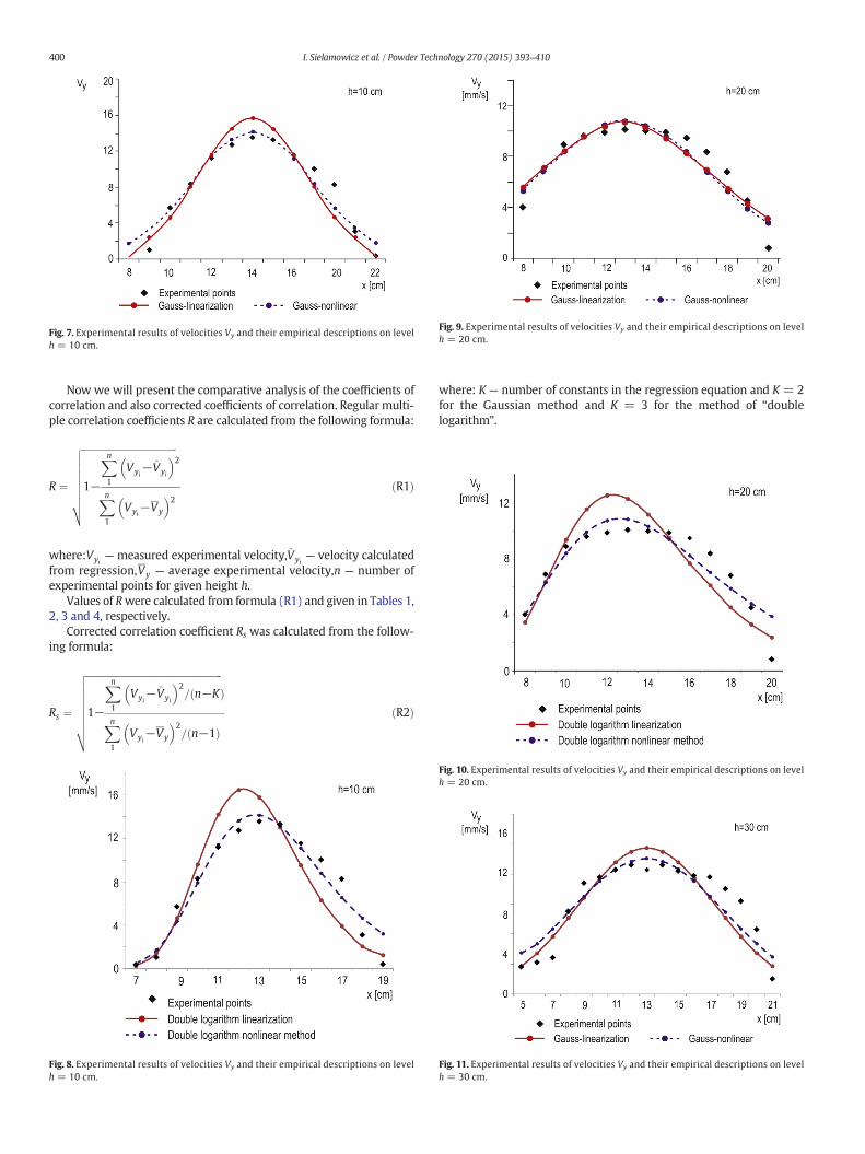
Fig. 9. Experimental results of velocities Vy and their empirical descriptions on levelh = 20 cm.
Fig. 7. Experimental results of velocities Vy and their empirical descriptions on levelh = 10 cm.
400 I. Sielamowicz et al. / Powder Technology 270 (2015) 393–410
Now we will present the comparative analysis of the coefficients ofcorrelation and also corrected coefficients of correlation. Regular multi-ple correlation coefficients R are calculated from the following formula:
R ¼
ffiffiffiffiffiffiffiffiffiffiffiffiffiffiffiffiffiffiffiffiffiffiffiffiffiffiffiffiffiffiffiffiffiffiffiffiffiffiffi
1−
Xn1
Vyi−V̂yi
� �2
Xn1
Vyi−Vy
� �2
vuuuuuuutðR1Þ
where:Vyi— measured experimental velocity,V̂yi
— velocity calculatedfrom regression,Vy — average experimental velocity,n — number ofexperimental points for given height h.
Values of Rwere calculated from formula (R1) and given in Tables 1,2, 3 and 4, respectively.
Corrected correlation coefficient Rs was calculated from the follow-ing formula:
Rs ¼
ffiffiffiffiffiffiffiffiffiffiffiffiffiffiffiffiffiffiffiffiffiffiffiffiffiffiffiffiffiffiffiffiffiffiffiffiffiffiffiffiffiffiffiffiffiffiffiffiffiffiffiffiffiffiffiffi
1−
Xn1
Vyi−V̂yi
� �2= n−Kð Þ
Xn1
Vyi−Vy
� �2= n−1ð Þ
vuuuuuuutðR2Þ
Fig. 8. Experimental results of velocities Vy and their empirical descriptions on levelh = 10 cm.
where: K — number of constants in the regression equation and K = 2for the Gaussian method and K = 3 for the method of “doublelogarithm”.
Fig. 10. Experimental results of velocities Vy and their empirical descriptions on levelh = 20 cm.
Fig. 11. Experimental results of velocities Vy and their empirical descriptions on levelh = 30 cm.

Fig. 14. Experimental results of velocities Vy and their empirical descriptions on levelh = 40 cm.
Table 5aComparison of the sums of the squares of differences of velocities for points located at8 cm ≤ x ≤ 17 cm.
h [cm] ∑ Vyi exp−Vyi emp
� �2
Gaussian method Method of double logarithm
Linearization Nonlinear methodof Gauss–Newton
Linearization Nonlinear method ofLevenberg–Marquardt
Fig. 12. Experimental results of velocities Vy and their empirical descriptions on levelh = 30 cm.
401I. Sielamowicz et al. / Powder Technology 270 (2015) 393–410
In Table 5b the coefficient of correlation R and corrected coefficientsRs are listed.
When analyzing the data given in Table 5b we can notice rathersmall differences between the regular multiple correlation coefficientsand the corrected ones for the Gaussianmethodwith the number of re-gression constants K=2. A little higher differences between these coef-ficients can be noticed for the method of “double logarithm” with thenumber of constants K = 3 especially for linearization.
5.2. Predicting velocities due to extrapolation
5.2.1. Predicting velocities due to the nonlinear Gaussian descriptionUsing formula (9) for level h = 50 cm we obtain values of parame-
ters A and B as follows:
A h ¼ 50cmð Þ ¼ 9:9 and B h ¼ 50cmð Þ ¼ −0:07: ð13Þ
Substituting formula (13) to formula (7a) we obtain the predictedvalues of velocities:
Vy ¼ 9:9 e−0:07x21 : ð14Þ
The calculations according to formula (14) and the experimentalresults are given in Table 6.
Fig. 13.Experimental results of velocities Vy and their empirical descriptions on levelh = 40 cm.
5.2.2. Predicting velocities Vy due to the nonlinear description of “the doublelogarithm” function
Using formula (12) we calculate the constant values A, B and C forlevel z = 50 cm
A 50cmð Þ ¼ −5:037;B 50cmð Þ ¼ 5:964;C 50cmð Þ ¼ −1:23: ð15Þ
Substituting the calculated values from formula (15) to formula (10a)we obtain formula to calculate velocities as follows:
Vy ¼ e−5:037þ5:964 ln x−1:23 ln 2x: ð16Þ
The calculated values of velocities according formula (16) arelisted in Table 7. For comparison and for more clear understanding
5 22.02 6.09 12.62 4.3110 30.56 16.85 70.22 9.1320 7.15 6.87 32.23 5.3530 9.75 3.27 8.46 2.5740 4.86 2.16 6.36 2.26
Table 5bComparative summary of correlation coefficients R and corrected correlation coefficientss RS.
Method of description h [cm]
5 10 20 30 40
“Gauss” linearization R 0.969 0.947 0.929 0.899 0.890Rs 0.965 0.942 0.922 0.892 0.889
“Gauss” nonlinear R 0.995 0.965 0.934 0.919 0.941Rs 0.991 0.962 0.928 0.914 0.937
“Double logarithm” linearization R 0.983 0.873 0.805 0.920 0.889Rs 0.978 0.846 0.760 0.884 0.873
“Double logarithm” nonlinear R 0.994 0.968 0.918 0.928 0.920Rs 0.992 0.961 0.900 0.917 0.908

Table 6The results of predicted and experimental velocities Vy for level h = 50 cm due to the Gaussian method.
x [cm] 6 7 8 9 10 11 12 13 14 15 16 17 18 19 20
Vy [mm/s]
Vy predicted 0.32 0.8 1.72 3.23 5.27 7.48 9.23 9.9 9.23 7.48 5.27 3.23 1.72 0.8 0.32Vy exp 6.4 6.6 7.1 7.5 7.5 7.5 7.6 7.6 7.6 6.6 7.4 6.6 6.3 5.8 3.5
Table 7Results of the predicted values of velocities for level h = 50 cm were calculated due to the method of “the double logarithm”.
x [cm] 6 7 8 9 10 11 12 13 14 15 16 17 18 19 20
Vy [mm/s]
Vy predicted 5.47 6.76 7.74 8.41 8.80 8.95 8.92 8.74 8.46 8.11 7.72 7.29 6.86 6.42 6.0Vy exp 6.4 6.6 7.1 7.5 7.5 7.5 7.6 7.6 7.6 6.6 7.4 6.6 6.3 5.8 3.5
402 I. Sielamowicz et al. / Powder Technology 270 (2015) 393–410
of the analysis, the valuesVy exp which were calculated in Table 6, arerepeated in Table 7.
5.3. Prediction velocities of flowing grains by using interpolation
5.3.1. Prediction velocities due to the nonlinear model of the Gaussian typeUsing formula (9) we also calculate the constant values A and B for
level z = 15 cm and their values are following:
A 15cmð Þ ¼ 14:82;B 15cmð Þ ¼ −0:0442: ð17Þ
Substituting the parameters from formula (17) to formula (7a) weobtain expression for velocity, from which we can calculate velocitiesfor corresponding values, x1:
Vy ¼ 14:82 e−0:0442x21 : ð18Þ
Table 8Results for interpolation obtained for level h = 15 cm due to the Gaussian method.
x [cm] 6 7 8 9 10 11 12
Vy [mm/s]
Vy interpol 1.7 3.02 4.91 7.31 9.96 12.42 14.18Vy exp 0 0.4 5.5 8.6 10.1 10.6 10.5
Table 9The results of predicted velocities by using interpolation for level h = 15 cm according to the
x [cm] 6 7 8 9 10 11 12
Vy [mm/s]
Vy interpol 0.29 1.17 3.02 5.73 8.69 11.18 12.66Vy exp 0 0.4 5.5 8.6 10.1 10.6 10.5
Table 10Values of the flow rate.
h[cm]
xmin xmax Flow rate Q [cm2/s]
Gaussian method
Nonlinearregression
Nonlinear regression according to formula (23) andconstants from Table 11
5 8 17 8.15 8.1710 6 20 10.23 10.0820 7 21 10.16 10.4730 4 22 10.52 10.5240 4 22 10.70 10.53
Detailed calculations of velocities due to formula (18) are given inTable 8, where we also put the experimental results for more clearcomparison and analysis.
5.3.2. Prediction velocities due to the nonlinear function of “the doublelogarithm”
Using formula (12) for level z=15 cmwe obtain values of constantparameters as follows:
A 15cmð Þ ¼ −40:35;B 15cmð Þ ¼ 33:66;C 15cmð Þ ¼ −6:63: ð19Þ
Substituting values from formula (19) to formula (10a), we obtainthe expression for velocities:
Vy ¼ e−40:35þ33:66 ln x−6:63 ln 2x: ð20Þ
13 14 15 16 17 18 19 20
14.82 14.18 12.42 9.96 7.31 4.91 3.02 1.710.5 10.5 9.4 9.9 8.6 5.5 4 0.25
method of “the double logarithm.”
13 14 15 16 17 18 19 20
13.0 12.36 11.04 9.39 7.67 6.06 4.66 3.5110.5 10.5 9.4 9.9 8.6 5.5 4.0 0.25
Method of “the double logarithm”
Nonlinearregression
Nonlinear regression according to formula (23) andconstants from Table 11
7.74 7.7510.34 10.2710.48 10.5910.50 10.5610.63 10.52
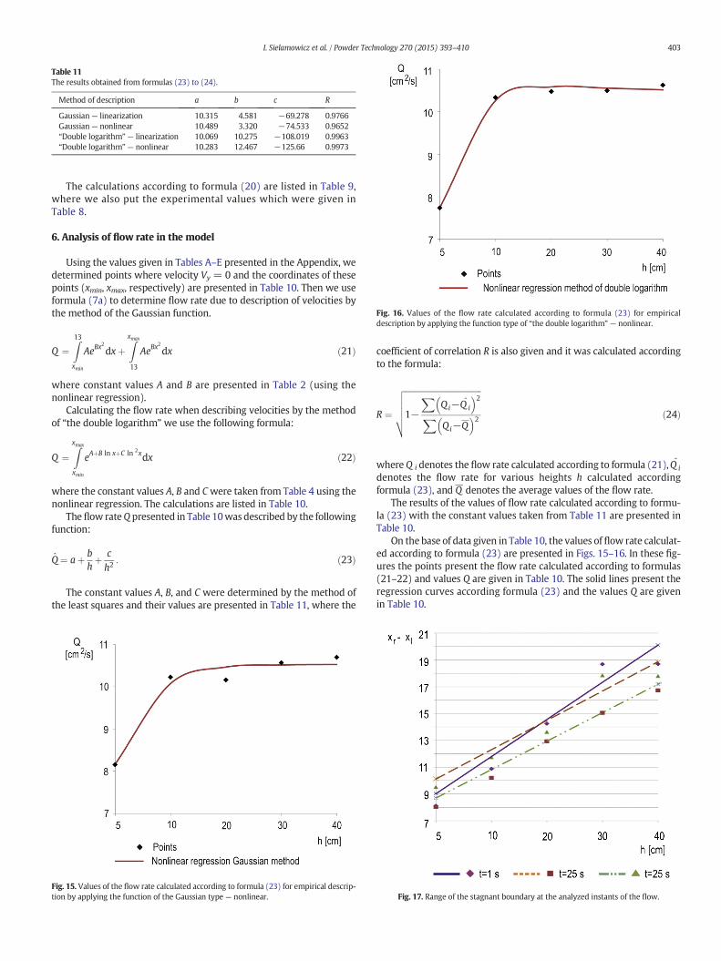
Fig. 16. Values of the flow rate calculated according to formula (23) for empiricaldescription by applying the function type of “the double logarithm” — nonlinear.
Table 11The results obtained from formulas (23) to (24).
Method of description a b c R
Gaussian— linearization 10.315 4.581 −69.278 0.9766Gaussian— nonlinear 10.489 3.320 −74.533 0.9652“Double logarithm” — linearization 10.069 10.275 −108.019 0.9963“Double logarithm” — nonlinear 10.283 12.467 −125.66 0.9973
403I. Sielamowicz et al. / Powder Technology 270 (2015) 393–410
The calculations according to formula (20) are listed in Table 9,where we also put the experimental values which were given inTable 8.
6. Analysis of flow rate in the model
Using the values given in Tables A–E presented in the Appendix, wedetermined points where velocity Vy = 0 and the coordinates of thesepoints (xmin, xmax, respectively) are presented in Table 10. Then we useformula (7a) to determine flow rate due to description of velocities bythe method of the Gaussian function.
Q ¼Z13
xmin
AeBx2
dxþZxmax
13
AeBx2
dx ð21Þ
where constant values A and B are presented in Table 2 (using thenonlinear regression).
Calculating the flow rate when describing velocities by the methodof “the double logarithm” we use the following formula:
Q ¼Zxmax
xmin
eAþB ln xþC ln 2xdx ð22Þ
where the constant values A, B and Cwere taken from Table 4 using thenonlinear regression. The calculations are listed in Table 10.
The flow rateQ presented in Table 10was described by the followingfunction:
Q̂ ¼ aþ bhþ ch2
: ð23Þ
The constant values A, B, and C were determined by the method ofthe least squares and their values are presented in Table 11, where the
Fig. 15. Values of the flow rate calculated according to formula (23) for empirical descrip-tion by applying the function of the Gaussian type — nonlinear.
coefficient of correlation R is also given and it was calculated accordingto the formula:
R ¼
ffiffiffiffiffiffiffiffiffiffiffiffiffiffiffiffiffiffiffiffiffiffiffiffiffiffiffiffiffiffiffiffiffiffiffiffiffiffi1−
XQi−Q ̂
i
� �2
XQi−Q
� �2
vuuuut ð24Þ
where Q i denotes the flow rate calculated according to formula (21),Q ̂i
denotes the flow rate for various heights h calculated accordingformula (23), and Q denotes the average values of the flow rate.
The results of the values of flow rate calculated according to formu-la (23) with the constant values taken from Table 11 are presented inTable 10.
On the base of data given in Table 10, the values of flow rate calculat-ed according to formula (23) are presented in Figs. 15–16. In these fig-ures the points present the flow rate calculated according to formulas(21–22) and values Q are given in Table 10. The solid lines present theregression curves according formula (23) and the values Q are givenin Table 10.
Fig. 17. Range of the stagnant boundary at the analyzed instants of the flow.

404 I. Sielamowicz et al. / Powder Technology 270 (2015) 393–410
7. Empirical description of stagnant zones boundaries
In Table L given in the Appendix a certain set of data is determined.They are x1 and x2, where x1 is the distance from the left side of themodel where velocity Vy is equal to zero and x2 is the distance fromthe right side of the model, where Vy is also equal to zero. Thesedistances were appointed for time instants t= 1, 25, 50 s and for levelsh = 5, 10, 20, 30, 40 cm.
On the base of values of x1 and x2 the difference x = x2 − x1 wascalculated where Vy ≠ 0. This difference was described by the linearfunction:
t ¼ 1 s½ �; x̂ ¼ x2−x1 ¼ 7:45þ 0:3166 h; r ¼ 0:965t ¼ 25 s½ �; x̂ ¼ x2−x1 ¼ 7:47þ 0:2433 h; r ¼ 0:988t ¼ 50 s½ �; x̂ ¼ x2−x1 ¼ 8:88þ 0:2485 h; r ¼ 0:964:
ð25Þ
Critical values rk = 0.878 for significance level α= 0.05 and for 5− 2 = 3 degrees of freedom according to publication [45].
In Fig. 17 the relations (25) are presented in the graphical form.
8. Conclusions
We can draw out a few significant conclusions and discuss them.They are the following:
1. Rejection “the thick” statistical errors calculated according toformulas (1) and (2), which are given in Tables A, B, C, D, and E inthe Appendix, and comparing with the critical value Kcrit leads tothe conclusion that it occurs rather seldom for locations of extremepoints where velocities are close to zero.
2. Comparing data given in Tables A–E with data in Tables F–J given intheAppendix, where the calculations of confidence interval for signif-icant levels α = 0.05 are presented, we see that time does not haveinfluence to velocities.
3. Description of velocities of flow by the function of the Gaussian type,i.e. formula (7a) and the function of “the double logarithm”, i.e.
Table BReadings at level h = 10 cm.
Time t [s] Vy [mm/s] for the distance from the left wall x [cm]
7 8 9 10 11 12
Before rejecting After rejecting
1 1 1 1 3 6 10 1525 0 0 0 0.5 4 13 14.550 0 1 1 6 10 11 11.575 0.25 2 2 9 11.5 12 12100 0.5 6 – 10 10 10 10.5K 0.936 1.907 1.414 1.455 1.524 1.544 1.315
α = 0.05, Kkr = 1.869.
Table AReadings at level h = 5 cm.
Time t [s] Vy [mm/s] for the distance from the left wall x [cm]
8 9 10 11 12
1 0.25 0.5 1 6 1525 0 0 2 10 1450 0 0.5 6 12 1875 0.25 3 6 11 19100 0.5 3 6 10 15K 1.009 1.213 1.437 1.862 1.44
α = 0.05, Kkr = 1.869.
formula (10a), is presented in this paper. The constant values tothese formulas were calculated by two methods, by the linearizationof these functions or by using the nonlinear regression. Figs. 5–14confirm that much better description, when calculating the constantvalues, was obtained when using nonlinear regression. Also datagiven in Table 5awhere the sumof squares of thedifferences of veloc-ities (using the nonlinear regression), is even a few times lower thanusing the linearization. Analyzingdata in Table 5awe see that the bet-ter description can be obtained by using the function of “the doublelogarithm”.
4. The above conclusion is further confirmed by comparison of Table 6with Table 7 and Table 8 with Table 9, respectively. Analyzing datain Tables 6 and 7 we see that using extrapolation it makes it possibleto obtain results of velocities much more close to the experimentalvalues when using the function of “the double logarithm”. Thesame conclusion can be drawn when analyzing data obtained by in-terpolation and presented in Tables 8 and 9. Especially this conclu-sion is true for the points located further from the symmetry axis ofthe silo.
5. Analyzing the curves presented in Figs. 15–16 we can see that theflow rate has different values in the volume up to h= 10 cm. Higherthan this level the flow rate is stabilized.
6. In Fig. 17 we analyzed the stagnant zone boundaries. They were line-ar as presented between level h = 5 and up to h = 40 cm. This factwas also proved by formula (25) where we see the high value ofthe Pearson coefficient of correlation and it is higher than the criticalvalue for the significant level α = 0.05.
Acknowledgments
The experiments were performed in the Institute of FundamentalTechnological Research PolishAcademyof Sciences using the equipmentand software for DPIV technique. Statistical analysis was done using thesoftware Statistica10.
Appendix
Statistical analysis of experimental results.
13 14 15 16 17 18 19
Before rejecting After rejecting
18 17.5 13 8 3.5 – 1 015 14.5 11 10 6 6 0.5 012 12.5 13 13 9 9 3 0.512 12.5 12 12 10.5 10.5 6 110.75 9.75 8.75 8.5 7.5 7.5 5 0.51.693 1.563 1.768 1.392 2.354 1.341 1.346 1.604
13 14 15 16 17
14.5 26 7 1 0.515 16 17 6 0.517 13 12.5 11 2.520 14 11 8 215 9 7 5.5 3.5
4 1.814 1.832 1.628 1.616 1.316

Table CReadings at level h = 20 cm.
Time t [s] Vy [mm/s] for the distance from the left wall x [cm]
3 4 5 6 7 8 9 10 11 12 13 14
Beforerejecting
Afterrejecting
Beforerejecting
Afterrejecting
Beforerejecting
Afterrejecting
Beforerejecting
Afterrejecting
Beforerejecting
Afterrejecting
1 0.5 0 1 0 2 0 3 0 4 0 5 5.5 8 9 10 10.25 1025 0 0 0 0 0 0 0 0 0 0 1 5 8 9.5 9.5 9.75 9.7550 0 0 0 0 0 0 0 0 0 0 3 8 9.5 9.75 9.75 9.75 9.7575 0 0 0 0 0 0 0 0 0 0 7 9 10 10.25 10.5 10.5 10.5K 1.728 0 1.732 0 1.732 0 2.261 0 1.732 0 1.341 1.195 1.254 1.397 1.509 1.354 1.633
Table C (continued)Readings at level h = 20 cm.
Time t [s] Vy [mm/s] for the distance from the left wall x [cm]
15 16 17 18 19 20 21 22 23 24 25 26
Beforerejecting
Afterrejecting
Beforerejecting
Afterrejecting
Beforerejecting
Afterrejecting
Beforerejecting
Afterrejecting
Beforerejecting
Afterrejecting
Beforerejecting
Afterrejecting
1 9.75 8.5 6.5 4.5 3 1.75 1 0 1 0 0.75 0 0.75 0 0.75 0 0.75 025 9.5 .5 9.5 8.25 4 0 0 0 0 0 0 0 0 0 0 0 0 050 9.5 9.5 8.75 8.5 6 0.25 0 0 0 0 0 0 0 0 0 0 0 075 10.75 10.5 9 6 5 1 0 0 0 0 0 0 0 0 0 0 0 0K 1.689 1.414 1.651 1.398 1.271 1.460 1.732 0 1.732 0 1.723 0 1.724 0 1.723 0 1.723 0
α = 0.05, Kkr = 1.689.
405I.Sielam
owicz
etal./Powder
Technology270
(2015)393
–410

Table DReadings at level h = 30 cm.
Time t [s] Vy [mm/s] for the distance from the left wall x [cm]
0 1 2 3 4 5 6 7 8 9 10 11 12 13
Beforerejecting
Afterrejecting
Beforerejecting
Afterrejecting
Beforerejecting
Afterrejecting
Beforerejecting
Afterrejecting
Beforerejecting
Afterrejecting
1 1 0 1 0 1 0 2 0 4 0 5 5.75 5.75 6 7 7.75 9 9 925 0 0 0 0 0 0 0 0 0 0 0 0 0.5 5.5 7.25 7.5 7.5 8 7.550 0 0 0 0 0 0 0 0 0 0 0.5 0.5 1 5 8 8.25 8.25 8.75 8.5K 1.422 0 1.422 0 1.414 0 1.415 0 1.416 0 1.410 1.412 1.407 1.225 1.365 1.365 1.226 1.365 1.330
Table D (continued)Readings at level h = 30 cm.
Time t [s] Vy [mm/s] for the distance from the left wall x [cm]
14 15 16 17 18 19 20 21 22 23 24 25 26
Beforerejecting
Afterrejecting
Beforerejecting
Afterrejecting
Beforerejecting
Afterrejecting
Beforerejecting
Afterrejecting
Beforerejecting
Afterrejecting
1 9 7.75 7 6.5 5.5 4 4 2.5 2 0 2 0 2 0 2 0 2 025 7.75 8.25 8 8 7.5 6.5 4 0 0 0 0 0 0 0 0 0 0 050 9 8.5 8.5 9 8 8 4.75 0.5 0 0 0 0 0 0 0 0 0 0K 1.409 1.346 1.283 1.295 0.505 1.315 1.412 1.380 1.414 0 1.414 0 1.414 0 1.414 0 1.414 0
α = 0.05, Kkr = 1.412.
406I.Sielam
owicz
etal./Powder
Technology270
(2015)393
–410

Table EReadings at level h = 40 cm.
Time t [s] Vy [mm/s] for the distance from the left wall x [cm]
0 1 2 3 4 5 6 7 8 9 10 11 12 13
Beforerejecting
Afterrejecting
Beforerejecting
Afterrejecting
Beforerejecting
Afterrejecting
Beforerejecting
Afterrejecting
Beforerejecting
Afterrejecting
1 1 0 2.5 0 3 0 4 0 5 0 5.75 6.5 6.5 7.5 8 8.25 9 8.75 8.525 0 0 0 0 0 0 0 0 0 0 0.25 2 6.25 6.25 6.75 6.75 6.75 6.5 7.2550 0 0 0 0 0 0 0 0 0.25 0 0.25 2.5 3.75 5 7 7.75 8 8.25 9K 1.422 0 1.416 0 1.415 0 1.416 0 1.526 0 1.412 1.405 1.409 1.224 1.329 1.33 1.272 1.378 1.41
Table E (continued)Readings at level h = 40 cm.
Time t [s] Vy [mm/s] for the distance from the left wall x [cm]
14 15 16 17 18 19 20 21 22 23 24 25 26
Beforerejecting
Afterrejecting
Beforerejecting
Afterrejecting
Beforerejecting
Afterrejecting
Beforerejecting
Afterrejecting
Beforerejecting
Afterrejecting
1 7.25 7.25 7 6.5 6 5 4 3.25 3.25 0 3.4 0 2.75 0 2.75 0 2.75 025 6.5 6.5 6.5 7 7 6 3 0 0 0 0 0 0 0 0 0 0 050 8.75 8.75 8.75 8.5 7.75 6.5 5.5 2 0 0 0 0 0 0 0 0 0 0K 1.359 1.337 1.378 1.376 1.283 1.33 1.293 1.307 2.386 0 2.386 0 1.414 0 1.414 0 1.414 0
α = 0.05, Kkr = 1.412.
407I.Sielam
owicz
etal./Powder
Technology270
(2015)393
–410
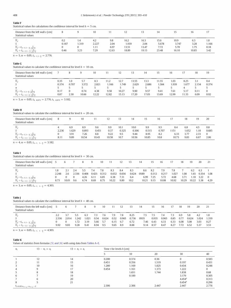
Table FStatistical values for calculations the confidence interval for level h = 5 cm.
Distance from the left wall x [cm]Statistical values
8 9 10 11 12 13 14 15 16 17
Vy 0.2 1.4 4.2 9.8 16.2 16.3 15.6 10.9 6.3 1.8S 0.187 1.319 2.227 2.04 1.939 2.04 5.678 3.747 3.28 1.166Vy−tn−1;1− α
2
Sffiffiffiffiffiffiffin−1
p 0 0 1.11 6.97 13.51 13.47 7.72 5.70 1.75 0.18Vy þ tn−1;1− α
2
Sffiffiffiffiffiffiffin−1
p 0.46 3.23 7.29 12.63 18.89 19.13 23.48 16.10 10.85 3.42
n = 5, α = 0.05, tn−1;1−α2= 2.776.
Table GStatistical values to calculate the confidence interval for level h = 10 cm.
Distance from the left wall x [cm]Statistical values
7 8 9 10 11 12 13 14 15 16 17 18 19
Vy 0.35 1.0 5.7 8.3 11.2 12.7 13.55 13.3 11.55 1.03 8.25 3.1 0.4S 0.374 0.707 3.572 2.821 1.166 1.749 2.629 2.686 1.584 1.939 1.677 2.154 0.374n 5 5 5 5 5 5 5 5 5 5 4 5 5Vy−tn−1;1−α
2
Sffiffiffiffiffiffiffin−1
p 0.17 0 0.74 4.38 9.58 10.27 9.90 9.57 9.41 7.61 5.17 0.11 0Vy þ tn−1;1−α
2
Sffiffiffiffiffiffiffin−1
p 0.87 2.30 10.66 12.22 12.82 15.13 17.20 17.03 13.69 12.99 11.33 6.09 0.92
n = 5, α = 0.05, t4, 0,975 = 2.776, t3, 0,975 = 3.182.
Table HStatistical values to calculate the confidence interval for level h = 20 cm.
Distance from the left wall x [cm]Statistical values
8 9 10 11 12 13 14 15 16 17 18 19 20
Vy 4 6.9 8.9 9.6 9.9 10.1 10.0 9.9 9.5 8.4 6.8 4.5 0.8S 2.236 1.629 0.893 0.451 0.37 0.325 0.306 0.515 0.707 1151 1.652 1.18 0.685Vy−tn−1;1− α
2
Sffiffiffiffiffiffiffin−1
p 0 3.91 7.26 8.8 9.22 9.5 9.44 8.95 8.2 6.33 3.77 2.33 0Vy þ tn−1;1− α
2
Sffiffiffiffiffiffiffin−1
p 8.11 9.89 10.54 10.43 10.58 10.7 10.56 10.85 10.8 10.73 9.83 6.67 2.06
n = 4, α = 0.05, tn−1; 1− α2= 3.182.
Table IStatistical values to calculate the confidence interval for level h = 30 cm.
Distance from the left wall x [cm]Statistical values
5 6 7 8 9 10 11 12 13 14 15 16 17 18 19 20 21
Vy 1.8 2.1 2.4 5.5 7.4 7.8 8.3 8.4 8.3 8.6 8.2 7.9 7.8 7 6.2 6.3 1S 2.248 2.6 2.336 0.408 0.425 0.312 0.632 0.656 0.624 0589 0.312 0.217 1.027 1.08 1.65 0.354 1.08Vy−tn−1;1− α
2
Sffiffiffiffiffiffiffin−1
p 0 0 0 4.26 6.11 6.85 6.38 7.31 6.4 6.99 7.25 5.72 4.68 3.71 1.18 3.22 0Vy þ tn−1;1− α
2
Sffiffiffiffiffiffiffin−1
p 8.73 10.01 9.6 6.74 8.69 8.75 10.22 9.89 10.2 10.21 9.15 10.08 10.92 10.29 10.22 5.38 4.29
n = 3, α = 0.05, tn−1; 1− α2= 4.303.
Table KValues of statistics from formulas (5) and (6) with using data from Tables A–E.
ni 13 − ni = xi 13 + ni = xi Time t for levels h [cm]
5 10 20 30 40
1 12 14 0.200 0.374 0.36 0 0.5832 11 15 0.451 0.356 1.519 0.197 0.4313 10 16 1.280 1.169 1.825 0.434 0.2464 9 17 0.454 1.161 1.373 1.222 05 8 18 1.651 1.744 1.838 0.686 7 19 0.189 3.179 0.3057 6 20 4.454x 0.3138 5 21 0.454x 0.296tcr:0:05:n13−ni
þn13þni−2 2.306 2.306 2.447 2.447 2.776
Table JStatistical values to calculate the confidence interval for level h = 40 cm.
Distance from the left wall x [cm]Statistical values
5 6 7 8 9 10 11 12 13 14 15 16 17 18 19 20 21
Vy 2.2 3.7 5.5 6.3 7.3 7.6 7.9 7.8 8.25 7.5 7.5 7.4 7.3 6.9 5.8 4.2 1.8S 2.536 2.014 1.242 1.021 0.54 0.624 0.52 0.965 0.736 0935 0.935 0.965 0.85 0.77 0.624 1.024 1.339Vy−tn−1;1− α
2
Sffiffiffiffiffiffiffin−1
p 0 0 1.72 3.19 5.66 5.7 6.15 6.7 6.72 7.46 6.43 6.33 6.33 6.08 5.08 3.03 0.27Vy þ tn−1;1− α
2
Sffiffiffiffiffiffiffin−1
p 9.92 9.83 9.28 9.41 8.94 9.5 9.65 8.9 8.88 9.14 8.57 8.47 8.27 7.72 6.52 5.37 3.53
n = 3, α = 0.05, tn−1; 1− α2= 4.303.
408 I. Sielamowicz et al. / Powder Technology 270 (2015) 393–410
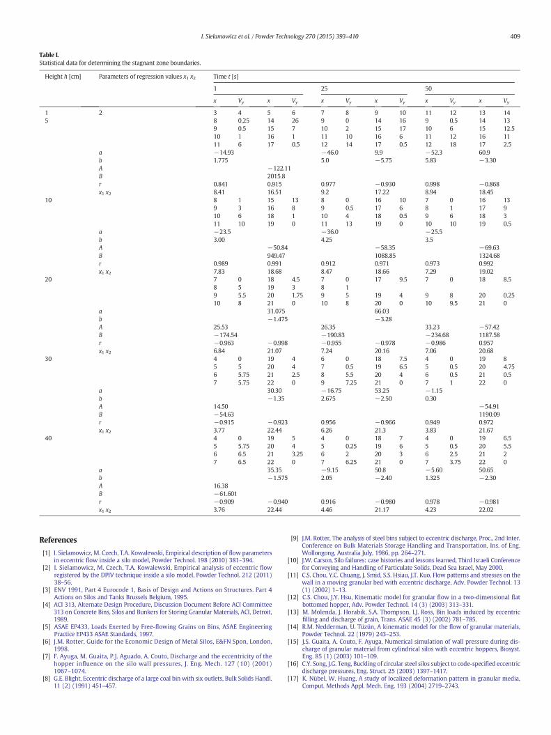
Table LStatistical data for determining the stagnant zone boundaries.
Height h [cm] Parameters of regression values x1 x2 Time t [s]
1 25 50
x Vy x Vy x Vy x Vy x Vy x Vy
1 2 3 4 5 6 7 8 9 10 11 12 13 145 8 0.25 14 26 9 0 14 16 9 0.5 14 13
9 0.5 15 7 10 2 15 17 10 6 15 12.510 1 16 1 11 10 16 6 11 12 16 1111 6 17 0.5 12 14 17 0.5 12 18 17 2.5
a −14.93 −46.0 9.9 −52.3 60.9b 1.775 5.0 −5.75 5.83 −3.30A −122.11B 2015.8r 0.841 0.915 0.977 −0.930 0.998 −0.868x1 x2 8.41 16.51 9.2 17.22 8.94 18.45
10 8 1 15 13 8 0 16 10 7 0 16 139 3 16 8 9 0.5 17 6 8 1 17 910 6 18 1 10 4 18 0.5 9 6 18 311 10 19 0 11 13 19 0 10 10 19 0.5
a −23.5 −36.0 −25.5b 3.00 4.25 3.5A −50.84 −58.35 −69.63B 949.47 1088.85 1324.68r 0.989 0.991 0.912 0.971 0.973 0.992x1 x2 7.83 18.68 8.47 18.66 7.29 19.02
20 7 0 18 4.5 7 0 17 9.5 7 0 18 8.58 5 19 3 8 19 5.5 20 1.75 9 5 19 4 9 8 20 0.2510 8 21 0 10 8 20 0 10 9.5 21 0
a 31.075 66.03b −1.475 −3.28A 25.53 26.35 33.23 −57.42B −174.54 −190.83 −234.68 1187.58r −0.963 −0.998 −0.955 −0.978 −0.986 0.957x1 x2 6.84 21.07 7.24 20.16 7.06 20.68
30 4 0 19 4 6 0 18 7.5 4 0 19 85 5 20 4 7 0.5 19 6.5 5 0.5 20 4.756 5.75 21 2.5 8 5.5 20 4 6 0.5 21 0.57 5.75 22 0 9 7.25 21 0 7 1 22 0
a 30.30 −16.75 53.25 −1.15b −1.35 2.675 −2.50 0.30A 14.50 −54.91B −54.63 1190.09r −0.915 −0.923 0.956 −0.966 0.949 0.972x1 x2 3.77 22.44 6.26 21.3 3.83 21.67
40 4 0 19 5 4 0 18 7 4 0 19 6.55 5.75 20 4 5 0.25 19 6 5 0.5 20 5.56 6.5 21 3.25 6 2 20 3 6 2.5 21 27 6.5 22 0 7 6.25 21 0 7 3.75 22 0
a 35.35 −9.15 50.8 −5.60 50.65b −1.575 2.05 −2.40 1.325 −2.30A 16.38B −61.601r −0.909 −0.940 0.916 −0.980 0.978 −0.981x1 x2 3.76 22.44 4.46 21.17 4.23 22.02
409I. Sielamowicz et al. / Powder Technology 270 (2015) 393–410
References
[1] I. Sielamowicz, M. Czech, T.A. Kowalewski, Empirical description of flow parametersin eccentric flow inside a silo model, Powder Technol. 198 (2010) 381–394.
[2] I. Sielamowicz, M. Czech, T.A. Kowalewski, Empirical analysis of eccentric flowregistered by the DPIV technique inside a silo model, Powder Technol. 212 (2011)38–56.
[3] ENV 1991, Part 4 Eurocode 1, Basis of Design and Actions on Structures. Part 4Actions on Silos and Tanks Brussels Belgium, 1995.
[4] ACI 313, Alternate Design Procedure, Discussion Document Before ACI Committee313 on Concrete Bins, Silos and Bunkers for Storing Granular Materials, ACI, Detroit,1989.
[5] ASAE EP433, Loads Exerted by Free-flowing Grains on Bins, ASAE EngineeringPractice EP433 ASAE Standards, 1997.
[6] J.M. Rotter, Guide for the Economic Design of Metal Silos, E&FN Spon, London,1998.
[7] F. Ayuga, M. Guaita, P.J. Aguado, A. Couto, Discharge and the eccentricity of thehopper influence on the silo wall pressures, J. Eng. Mech. 127 (10) (2001)1067–1074.
[8] G.E. Blight, Eccentric discharge of a large coal bin with six outlets, Bulk Solids Handl.11 (2) (1991) 451–457.
[9] J.M. Rotter, The analysis of steel bins subject to eccentric discharge, Proc., 2nd Inter.Conference on Bulk Materials Storage Handling and Transportation, Ins. of Eng.Wollongong, Australia July, 1986, pp. 264–271.
[10] J.W. Carson, Silo failures: case histories and lessons learned, Third Israeli Conferencefor Conveying and Handling of Particulate Solids, Dead Sea Israel, May 2000.
[11] C.S. Chou, Y.C. Chuang, J. Smid, S.S. Hsiau, J.T. Kuo, Flow patterns and stresses on thewall in a moving granular bed with eccentric discharge, Adv. Powder Technol. 13(1) (2002) 1–13.
[12] C.S. Chou, J.Y. Hsu, Kinematic model for granular flow in a two-dimensional flatbottomed hopper, Adv. Powder Technol. 14 (3) (2003) 313–331.
[13] M. Molenda, J. Horabik, S.A. Thompson, I.J. Ross, Bin loads induced by eccentricfilling and discharge of grain, Trans. ASAE 45 (3) (2002) 781–785.
[14] R.M. Nedderman, U. Tüzün, A kinematic model for the flow of granular materials,Powder Technol. 22 (1979) 243–253.
[15] J.S. Guaita, A. Couto, F. Ayuga, Numerical simulation of wall pressure during dis-charge of granular material from cylindrical silos with eccentric hoppers, Biosyst.Eng. 85 (1) (2003) 101–109.
[16] C.Y. Song, J.G. Teng, Buckling of circular steel silos subject to code-specified eccentricdischarge pressures, Eng. Struct. 25 (2003) 1397–1417.
[17] K. Nübel, W. Huang, A study of localized deformation pattern in granular media,Comput. Methods Appl. Mech. Eng. 193 (2004) 2719–2743.
410 I. Sielamowicz et al. / Powder Technology 270 (2015) 393–410
[18] J.F. Chen, J.M. Rotter, J.Y. Ooi, Z. Zhong, Flow patternsmeasurement in a full scale silocontaining iron ore, Chem. Eng. Sci. 60 (2005) 3029–3041.
[19] J. Nielsen, V. Askegaard, Scale errors in model tests in granular media with specialreference to silo models, Powder Technol. 16 (1) (1977) 123–130.
[20] H.E. Wright, G.F. Cudahy, J.T. Van Kuren, Degradation of laser beam by a twodimensional turbulent jet, AIAA J. 17 (10) (1979) 1091–1097.
[21] J. Nielsen, N.O. Kristiansen, Related measurements of pressure condition in full scalebarley silo and in silo model, Proc. of the International Conference on Design of Silosfor Strength and Flow, University of Lancaster, Powder Advisory Centre, September1980.
[22] J. Munch-Andersen, J. Nielsen, Size effects in large grain silos, Bulk Solids Handl. 6(1986) 885–889.
[23] J. Nielsen, Pressures from flowing granular solids in silos, Philos. Trans. R. Soc. Lond.Ser. A 356 (1747) (1998) 2667–2684.
[24] J.F. Chen, J.M. Rotter, J.Y. Ooi, A review of numerical prediction methods for silo wallpressures, Adv. Struct. Eng. 2 (2) (1999) 119–135.
[25] J.F. Chen, K.F. Zhang, J.Y. Ooi, J.M. Rotter, Visualisation of solids flow in a full scalesilo, Proc., 3rd European Symposium on Storage and Flow of Particulate Solids(Janssen Centennial), Nuremberg, Germany, 21–23 March, 1995, pp. 427–436.
[26] J.F. Chen, Interpretation of Flow and Pressures in Full Scale Silos(Ph.D. Thesis)University of Edinburg, 1996. (678 pp.).
[27] A. Medina, J.A. Cordova, E. Luna, C. Treviño, Velocity filed measurements in granulargravity flow, Phys. Lett. A 250 (1998) 111–116.
[28] R.M. Lueptow, A. Akonur, T. Shinbrot, PIV for granular flow, Exp. Fluids 28 (2)(2000) 183–186.
[29] A.J. Waters, A. Drescher, Modelling plug flow in bins/hoppers, Powder Technol. 113(2000) 168–175.
[30] M. Ostendorf, J. Schwedes, Application of particle image velocimetry for velocitymeasurements during silo discharge, Powder Technol. 158 (2005) 69–75.
[31] J.U. Böhrnsen, H. Antes, M. Ostendorf, J. Schwedes, Silo discharge: measurement andsimulation of dynamic behaviour in bulk solids, Chem. Eng. Technol. 27 (2004)71–76.
[32] I. Sielamowicz, S. Błoński, T.A. Kowalewski, Optical technique DPIV inmeasurementsof granular material flow, part 1 of 3—plane hoppers, Chem. Eng. Sci. 60 (2) (2005)589–598.
[33] I. Sielamowicz, S. Błoński, T.A. Kowalewski, Optical technique DPIV inmeasurementsof granular material flow, part 2 of 3 — converging hoppers, Chem. Eng. Sci. 61(2006) 5307–5317.
[34] I. Sielamowicz, Experimental analysis of granularmaterial flows using the techniqueof digital particle image velocimetry, Eng. Trans. 53 (2) (2005) 195–227.
[35] D.A. Steingart, J.W. Evans, Measurements of granular flow in two-dimensionalhoppers by particle image velocimetry. Part I: experimental method and results,Chem. Eng. Sci. 60 (2005) 1043–1051.
[36] P.M. Blair-Fish, P.L. Bransby, Flow Patterns andWall Stresses in a Mass-Flow Bunker,1973. 17–26 (Error! Not a valid link).
[37] A. Drescher, T.W. Cousens, P.L. Bransby, Kinematics of the mass flow of granularmaterial through a plane hopper, Geotechnique 28 (1) (1978) 27–42.
[38] J.Y. Ooi, J.F. Chen, J.M. Rotter, Measurement of solids flow patterns in a gypsum silo,Powder Technol. 99 (3) (1998) 272–284.
[39] J. Choi, A. Kudrolli, M.Z. Bazant, Velocity profile of granular flow inside silos andhoppers, J. Phys. Condens. Matter 17 (2005) S2533–S2548.
[40] C.S. Chou, J.Y. Hsu, Y.D. Lau, Flow patterns and stresses on the wall in a two-dimensional flat-bottomed bin, J. Chin. Inst. Eng. Trans. Chin. Inst. Eng. Ser. A 26(4) (2003) 397–408.
[41] H. de Clercq, Investigation into stability of a silo with concentric and eccentricdischarge, Civ. Eng. S. Afr. 32 (3) (1990) 103–107.
[42] M. Wójcik, G.G. Enstad, M. Jecmenica, Numerical calculations of wall pressures andstresses in steel cylindrical silos with concentric and eccentric hoppers, J. Part. Sci.Technol. 21 (3) (2003) 247–258.
[43] G.M. Quenot, J. Pakleza, T.A. Kowalewski, Particle image velocimetry with opticalflow, Exp. Fluids 25 (1998) 177–189.
[44] I. Likiesh, J. Liaga, Osnownyje tablicy matiematiczeskoj statistiki, Моskwa,1985.
[45] W. Volk, Applied Statistics for Engineers, second edition McGraw-Hill, 1979.