compaction for two models of logarithmic-depth …

COMPACTION FOR TWO MODELS OF LOGARITHMIC-DEPTH TREES:ANALYSIS AND EXPERIMENTS

OLIVIER BODINI, ANTOINE GENITRINI, BERNHARD GITTENBERGER, ISABELLA LARCHER,AND MEHDI NAIMA

Abstract. We are interested in the quantitative analysis of the compaction ratio for two clas-sical families of trees: recursive trees and plane binary increasing trees. These families aretypical representatives of tree models with a small depth. Once a tree of size n is compactedby keeping only one occurrence of all fringe subtrees appearing in the tree the resulting graphcontains only O(n/ lnn) nodes. This result must be compared to classical results of compactionin the families of simply generated trees, where the analogous result states that the compactedstructure is of size of order n/

√lnn. The result about the plane binary increasing trees has

already been proved, but we propose a new and generic approach to get the result. Finally,an experimental study is presented, based on a prototype implementation of compacted binarysearch trees that are modeled by plane binary increasing trees.

Keywords: Analytic Combinatorics; Tree compaction; Common subexpression recognition;Increasing trees; Binary search trees

1. Introduction

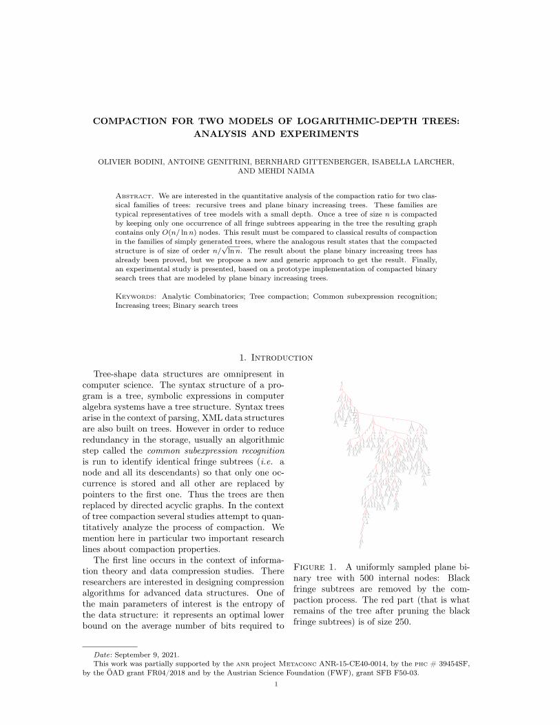
Figure 1. A uniformly sampled plane bi-nary tree with 500 internal nodes: Blackfringe subtrees are removed by the com-paction process. The red part (that is whatremains of the tree after pruning the blackfringe subtrees) is of size 250.

Tree-shape data structures are omnipresent incomputer science. The syntax structure of a pro-gram is a tree, symbolic expressions in computeralgebra systems have a tree structure. Syntax treesarise in the context of parsing, XML data structuresare also built on trees. However in order to reduceredundancy in the storage, usually an algorithmicstep called the common subexpression recognitionis run to identify identical fringe subtrees (i.e. anode and all its descendants) so that only one oc-currence is stored and all other are replaced bypointers to the first one. Thus the trees are thenreplaced by directed acyclic graphs. In the contextof tree compaction several studies attempt to quan-titatively analyze the process of compaction. Wemention here in particular two important researchlines about compaction properties.

The first line occurs in the context of informa-tion theory and data compression studies. Thereresearchers are interested in designing compressionalgorithms for advanced data structures. One ofthe main parameters of interest is the entropy ofthe data structure: it represents an optimal lowerbound on the average number of bits required to

Date: September 9, 2021.This work was partially supported by the anr project Metaconc ANR-15-CE40-0014, by the phc # 39454SF,

by the ÖAD grant FR04/2018 and by the Austrian Science Foundation (FWF), grant SFB F50-03.1

2 O. BODINI, A. GENITRINI, B. GITTENBERGER, I. LARCHER, AND M. NAIMA

represent the data structure: see for example [10] for an introduction to the subject. For trees,the entropy of some models of plane trees1 has been studied in particular in [26, 9, 20].

An analysis of a model of non-plane binary trees has been presented in [9]. The authors focuson the number of symmetry nodes (internal nodes having two isomorphic subtrees as children)and its relation with Rényi entropy. In all investigations of that kind, the probability distributionused for the tree model is central. The aforementioned work [9] is focusing on a growing treemodel that is also seen as the classical binary search tree distribution model. Likewise, it can berephrased as the binary increasing tree model we will deal with in Section 3, as it was alreadypointed out in [4]. We are, however, interested in different aspects of these trees (see below formore details).

The second line of research has been started by the seminal paper of Flajolet et al [19]. Inthis paper the authors consider the compaction ratio of classical binary trees compared with theircorresponding compacted structures. They prove, starting from a large binary tree of size n (con-taining n nodes) and then compacting it, then the average size of the compacted result is αn/

√lnn

with a computable constant α. In the end of the paper the authors finally state that their analysisis fully adapted to all families of simply generated trees as defined by Meir and Moon in theirfundamental paper [28] and thus for all kinds of tree structures we mentioned above as examples,we get the same kind of ratio for the compaction. In Figure 1 we have represented a uniformlysampled binary tree with 500 internal nodes. If we compact it then all the fringe subtrees in blackare removed and only the red structure is kept with addition of several pointers (that are notrepresented in the figure). The remaining red tree is of size 250. We recall that in the context ofsimply generated trees of size n, the typical depth is of order

√n (this is the case for the binary

trees). Bousquet-Mélou et al. [7] present the complete proof for the compaction quantitative anal-ysis of simply generated tree families and apply it experimentally on XML-trees. Finally, in [32]the authors are interested in the number of fringe subtrees with at least r occurrences in a randomsimply generated tree. This approach is an extension of the previous results where it was dealtwith subtrees appearing at least once (thus for r = 1).

But there are also several other kinds of tree structures that cannot be modeled through theconcept of simply generated trees. In particular, we have in mind all structures used for searching,and thus usually with a small depth of order lnn for a whole structure of size n. The classicalbinary search trees (bst), red-black trees or AVL trees belong to these families. But we canalso point out priority heaps like binary or binomial heaps. The reader can refer for example toKnuth’s book [24] for details about all these structures. In this context, all nodes contain differentlabels (or information) and thus the compaction process as described before has no effect (no twosubtrees are identical due to the labeling). But, if we remove the labels from the nodes, then atree structure remains whose typical depth is of order lnn for n nodes. Hence we can compact thetree structure. In Figure 2 we have depicted a binary search tree structure of size 500. Once the

Figure 2. A uniformly sampled (plane) binary search tree structure with 500 internalnodes: Black fringe subtrees are removed by the compaction. The red part is only ofsize 172.

1Plane trees are such that the descendants of a node are ordered contrary to non-plane trees where the descen-dants are seen as a set instead of a sequence of subtrees.

COMPACTION FOR TWO MODELS OF LOGARITHMIC-DEPTH TREES: ANALYSIS AND EXPERIMENTS 3

structure is compacted, it remains a tree with 172 nodes (represented in red).Our study focuses on the number of non-isomorphic subtrees in a tree and this corresponds also

to the size of the compacted tree (also called minimal DAG representation in [33]). This parameteris different from the study of symmetry nodes mentioned above (see [9]), since there symmetrieshappen if an internal node has two isomorphic children (a local symmetry) whereas the numberof non-isomorphic subtrees of a tree is capturing a global symmetry. Using the results in [9] todesign and analyze a data compression algorithm leads to constant compression rate on average,as was already shown in [16]. In our case, we gain on average at least a logarithmic factor.

For both investigations, a Riccati-like functional-differential equation must be analyzed. But,not only the equations in [9] and in Section 3 are different, but the global nature of the parameterof our interest is reflected by the need of uniform asymptotics, which required a delicate singularityanalysis.

In this paper, we analyze the underlying unlabeled tree structure of a plane and a non-planemodel of increasingly labeled trees, namely increasing binary trees and recursive trees. For thesetwo models of trees picking a tree uniformly at random and erasing the labels from it givesan unlabeled plane binary tree or an unlabeled non-plane general tree (also called Pólya tree).However, for each model the probability distribution of the resulting unlabeled tree is non-uniform.The distribution on plane binary trees we use is the same as the one of [9, 26]. Even if the analyzedparameters are not the same, for all such studies the mathematical tools are based on differentialequation analyses due to the underlying distribution on trees.

Finally, another way to reach the non-uniform distribution is as a very simple natural evolutionprocess. First let us mention the plane binary tree model: start with a single node, and at eachstep select randomly one of the leaves (external node) and replace with a binary node. While forPólya trees, start with a node and at each step select randomly one of the nodes and append anew leaf to it.

We are interested in the analysis of the compaction ratio, relating the tree size and its minimalDAG size as in [33] for two families of trees that are not simply generated trees. The first familyconsists of recursive trees (Section 2). The family has been introduced by Moon [30] and furtherstudied by Meir and Moon in the 70s [28]. Their motivation was to present a tree model forthe spread of epidemics. The second tree family we are interested in is the class of plane binaryincreasing tree (Section 3). It corresponds to the tree model for binary search trees. Both familieshave been extensively studied in the last two decades with probabilistic methods [27, 12, 8, 14] aswell as with combinatorial ones [4, 25, 31].

For recursive trees and binary increasing trees, informally speaking we prove that, asymptoti-cally, if a tree of size n is compacted, then the resulting structure has on average size O (n/ lnn),with a lower bound of Ω(

√n).

In the context of binary increasing trees the result has already been derived. The upper boundO (n/ lnn) was proved in [16] as a specific result in the context of patterns in random binarysearch trees. The proof is based on some bivariate generating function analysis in the AnalyticCombinatorics context. The stronger Θ-result has then been proved in [11] based on a preliminaryresult in [15]. These papers are based on probability theory rather than Analytic Combinatorics.But recently other authors [2, 3] presented new proofs based on Analytic Combinatorics. We,however, decided to briefly present a further proof based on Analytic Combinatorics, as it is genericin the following sense: the same approach is valid for recursive trees as well as for binary increasingtrees. Especially in order to derive our results, we analyze a perturbation of the differentialequation defining the tree models, observing that analogous functions related to the increasinglabeling of the tree structure are central in both tree models. And under the assumption that acertain experimentally supported conjecture is true, almost the same proof can be used to improvethe lower bound and get a Θ-result for both classes.

We thus remark that such a kind of trees are compacted in a more efficient way (in the sense ofthe number of remaining nodes) than simply generated trees. Finally, we end the paper (Section 4)with a section dedicated to the compaction of binary search trees (bst) in practice, in order toexhibit the way we can compact the tree structure, but by keeping some extra information we loseno information (about the labeling of the initial bst). An experimental study is provided by using


a prototype in python for our new data structure, the compacted bst. The experiments are veryencouraging for the development of such new compacted search tree structures.

So, as a synthesis, Section 2 is dedicated to the compaction analysis of recursive trees. ThenSection 3 contains the key elements to derive the same result for binary increasing trees andfinally, Section 4 presents an experimental approach to verify the latter result in the context ofdata structures.

Remarks. We note that for all figures we present, we use a postorder traversal of the tree represen-tation in order to compact them. However, whatever traversal is chosen, the quantitative resultsare always identical.

Recall that the size of the compacted tree also equals the number of distinct unlabeled fringesubtrees appearing in the original tree.

2. Recursive trees

The class of recursive trees has been studied by Meir and Moon [28]. These trees are modelsin several contexts as e.g. for the study of epidemic spreads, and thus many quantitative studyhave focused on this family. Some details are presented either in [13] or in [18]. Using the classicaloperators from Analytic Combinatorics, recursive trees can be specified by the so-called boxedproduct, or Greene operator,

T = Z ? Set(T ),

meaning that the structure of a recursive tree (in the class T ) is defined as a root Z attached to aset of recursive trees (the set may be empty, then Z is a leaf) and such that the whole structureis canonically labeled (1, 2, . . . , up to the size). The box in the boxed product indicates that thelowest label goes into the left component (the atom in this case). The atoms Z in the structureare therefore labeled increasingly on each path from the root of the tree to any leaf. See [18,Section II.6.3] for details about the constraint labeling operators. The class of recursive trees isalso presented in [13, Section 1.3].

1

6

7

9 11

17

2

4

5

16

12

3

138

1410 15

Figure 3. Example of a recursive tree of size 17

On the left side of Figure 3 we have represented a recursive tree of size 17. The children of anode are put in lexicographic order of their root labels. We remark that the unlabeled structuresunderlying the fringe subtrees rooted at 4 and 7 have the same unlabeled non-plane structure.And obviously the leaves are also identical. So, in the middle of the figure we represent with blackedges the fringe subtrees whose unlabeled non-plane structure has already been seen through apostorder traversal of the leftmost tree. Finally, on the right side of the figure we replace themultiple occurrences of a subtree by pointers to the first occurrence.

In Figure 4 we have represented a recursive tree structure containing 5,000 nodes on the leftside. It has been uniformly sampled among all trees with the same size. The original root of thetree is represented using a small circle . On the right side we have depicted the nodes that arekept after the compaction of the latter tree. Only 663 nodes remain.

We define the exponential generating function T (z) =∑n≥1 Tn

zn

n! , where Tn corresponds tothe number of trees containing n nodes i.e. of size n. Using the now classical symbolic methodfrom Analytic Combinatorics, from the latter unambiguous specification we deduce the following


Figure 4. (left) A uniformly sampled non-plane recursive tree of size 5,000: Blackfringe subtrees are removed by the compaction. (right) The red part is of size 663.

functional equation satisfied by T (z):

T (z) =

∫ z

0

exp(T (v)) dv.

The unique power series solution satisfying T (0) = 0 is

T (z) = ln1

1− z,

whose dominant singularity is ρ = 1. Finally, we get the value Tn = (n− 1)!.Let Tn be the class of recursive trees of size n; the size of a tree τ is defined as the number of its

nodes and is denoted by |τ |. Let Xn be the size of the compacted tree corresponding to a randomrecursive tree τ of size n. In other words, Xn is the number of distinct fringe subtree shapes in τ .We define P as the set of Pólya trees, i.e., non-plane unlabeled trees such that the degrees of theirnodes are arbitrary. This class of trees is presented in detail in Drmota’s book [13, Section 1.2.5].and it corresponds to the possible shapes of the recursive trees, once the increasing labeling hasbeen removed. We denote by P≤n the set of all Pólya trees with size at most n. Then we have

E (Xn) =∑t∈P≤n

P(t occurs as subtree of τ) =∑t∈P≤n

1− P(t does not occur as subtree of τ). (1)

Recall that the tree t corresponds to a tree shape, it is unlabeled, while τ is a recursive tree andtherefore is increasingly labeled.

Now, for a given Pólya tree t ∈ P let us consider a perturbed combinatorial class St thatcontains all recursive trees except for those that contain a t-shape as a (fringe) subtree. Thecorresponding exponential generating function satisfies the differential equation

S′t(z) = exp(St(z))− P ′t (z), (2)

where Pt(z) = `(t) z|t|

|t|! , with `(t) denoting the number of ways to increasingly label the tree shape t.


So, using (1) we obtain

E (Xn) =∑t∈P≤n

(1− P(t does not occur as shape of a fringe subtree of τ))

=∑t∈P≤n

(1− [zn]St(z)

[zn]T (z)

). (3)

Therefore, the problem is now essentially reduced to the analysis of the asymptotic behavior of[zn]St(z).

Solving (2) we obtain the exponential generating function

St(z) = ln

(1

1−∫ z

0exp(−Pt(v)) dv

)− Pt(z). (4)

Thus, for the dominant singularity ρt of St(z), the following equation must hold:∫ ρt

0

exp(−Pt(v)) dv = 1. (5)

As exp(−Pt(v)) < 1 for positive v, the dominant singularity ρt is greater than 1. Recall that ρdenotes the dominant singularity of T (z), thus ρ = 1 and therefore we write ρt = ρ(1+ εt) = 1+ εtwith suitable εt > 0.

Notations. Before we proceed, let us introduce some frequently used notations: For the size andthe weight of a Pólya tree t we use

k := |t| and w(t) :=`(t)

|t|!,

respectively. Moreover, let

G(z) :=

∫ z

0

e−Pt(v) dv =

∫ z

0

e−w(t)vk dv,

if z ≥ 0 and its complex continuation if z is not a nonnegative real number. With this notation(5) reads as G(1 + εt) = 1. By expanding the integrand, we obtain

G(z) =∑`≥0

(−w(t))`z`k+1

(`k + 1) · `!,

which shows that G(z) is an entire function.

How to proceed. Taking a random recursive tree of size n, we are interested in the asymptoticbehavior of the size of the compacted tree issued from the compaction of the recursive one. Inorder to obtain bounds for this compacted size we proceed as follows: First, in Lemma 1, wecompute a upper bound for ρt.

Then, in Proposition 1, we provide uniform asymptotics for the n-th coefficient of the generatingfunction St(z) when n tends to infinity, thereby showing that the error term is sufficiently smallfor what is needed later on.

The average size of a compacted tree corresponding to a random recursive tree is expressed asa sum over the forbidden trees. Thereby, the two cases where the size k of the forbidden tree tis smaller or larger than log n are treated in a different way: Upper bounds for the size of thecompacted tree are derived in Proposition 2 (small trees) and Proposition 3 (large trees). Finally,Proposition 4, gives a (crude) lower bound for the size of the compacted tree.

Lemma 1. Let St(z) be the generating function of the perturbed combinatorial class ( cf. Equa-tion (2)) of recursive trees that do not contain a subtree of shape t and ρt be the dominant singu-larity of St(z) ( cf. Equation (5)). Furthermore, let k = |t| and w(t) = `(t)/k! where `(t) denotesthe number of possible increasing labelings of the Pólya tree t. Then

ρt = 1 + εt < 1 +2w(t)

k.


Proof. First observe that the number of increasing labelings of the Pólya tree t is bounded by(k − 1)!, which gives the very crude bound w(t) ≤ 1/k which is valid for any tree t.

Next, as ρt satisfies G(1 + εt) = 1, it suffices to show the inequality G(

1 + 2w(t)k

)> G(1 + εt).

We show the equivalent inequality G(

1 + 2w(t)k

)−G(1) > G(1 + εt)−G(1): If k = 2, then t is a

path of length one and therefore w(t) = 1/2. This gives explicitly∫ 3/2

1e−v

2/2 dv > 1/6 which iseasily verified.If k ≥ 3, then we have the lower bound

G

(1 +

2w(t)

k

)−G(1) ≥ 2w(t)

kexp

(−w(t)

(1 +

2w(t)

k

)k)

≥ 2w(t)

kexp

(−w(t)

(1 +

2

k2

)k),

because w(t) ≤ 1/k. Then for k ≥ 3 we have(1 + 2

k2

)k< 2 and again, since w(t) ≤ 1/k, we obtain

2e−2/3 > 1 and thus

G

(1 +

2w(t)

k

)−G(1) ≥ w(t)

k· 2e−2w(t) >

w(t)

k + 1.

On the other hand, we have

G(1 + εt)−G(1) = 1−∫ 1

0

e−w(t)vk dv ≤ 1−∫ 1

0

(1− w(t)vk) dv =w(t)

k + 1,

which implies the assertion.

With a similar reasoning as in the above proof a lower bound for ρt can be shown:

Corollary 1. With the notations of Lemma 1 we have the following estimate:

ρt > 1 +w(t)

k + 1.

Corollary 2. With the notations of Lemma 1 we have the following asymptotic relation:

ρt = 1 + εt ∼ 1 +w(t)

k, as k →∞.

Proof. Write G(z) as G(z) = z +R(z) with

R(z) =∑`≥1

(−w(t))`z`k+1

(`k + 1) · `!(6)

As ρt = 1 + εt is the smallest positive solution of G(z) = 1, it is the smallest positive zero ofz − 1 +R(z). From Lemma 1 we know that εt = O

(1/k2

)and thus ρkt ∼ 1, as k tends to infinity,

and R(ρt) = w(t)ρk+1t /(k + 1) +O

(1/k3

). This implies

εt ∼w(t)

k + 1ρk+1t ∼ w(t)

k,

as desired.

Remark. In the paper [21], which is related to pattern exclusion in recursive trees, the same resultabout the singularity ρt is proved. Using more terms of the expansion of G(z), it is possible toderive a more accurate asymptotic expression for εt (in principle up to arbitrary order). As anexample, we state

ρt = 1 +w(t)

k + 1+

w(t)2(3k + 1)

(k + 1)(4k + 2)+w(t)3(29k3 + 32k2 + 10k + 1)

6(k + 1)2(2k + 1)(3k + 1)+O

(w(t)4

k

).


Note that in the sequel we will have to evaluate the coefficient [zn]St(z) for n tending to infinityand |t| tending to infinity with n as well. Thus a standard transfer lemma in the sense of Flajoletand Odlyzko [17] is not sufficient. We need a tight and uniform error term. In order to find this,we need to know where the second dominant singularity is, or rather where we can be sure thatthere will not be any singularity. The next lemma provides information about an eventually largeenough singularity-free region.

Lemma 2. Let St(z) be the generating function of the perturbed class of recursive trees definedin (4). Then St(z) has no singularity in the domain

ρt < |z| < 1 +ln(1/w(t)) + ln ln ln(1/w(t))

k.

Proof. Recall that by (4) we have

St(z) = ln

(1

1−G(z)

)− Pt(z).

Since G(z) is an entire function, the singularities of St(z) are exactly the zeros of G(z) − 1.Therefore, consider z0 such that G(z0) = 1 and write G(z) = z +R(z) with R(z) as in (6). Thenthe chosen number z0 must satisfy the inequality

|R(z0)| ≤ |z0|k + 1

∑`≥1

|w(t)|`|z0|k`+1

`!<

1

k(e|w(t)||z0|k − 1). (7)

The first step is to show that G(z)−1 does not have any zeros (except ρt) in a sufficiently largedomain, i.e. that either z0 = ρt or |z0| is large. We have to approach this in two steps.

Case 1: Assume first that |z0| ≤ 1 + α ln(1/w(t))k for some α < 1. As the dominant singularity

of St(z) is ρt and ρt > 1, we must have |z0| > 1. Thus, the upper bound on |z0| implies |z0|k ≤exp (α ln(1/w(t))) = (1/w(t))α = o(1/w(t)) and by (6) we obtain then

1− z0 = R(z0) ∼ −w(t)

kzk0 = o

(1

k

). (8)

This implies further that zk0 ∼ 1, hence z0 is asymptotically equal to a k-th root of unity. Butthen z0 = ρt, because the distance between the other k-th roots of unity and 1 is greater than1/k, which contradicts (8).

Case 2: Now, assume that |z0| = 1+η with α ln(1/w(t))/k < η ≤ (ln(1/w(t))+ln ln ln(1/w(t))−δ)/k for some arbitrary but small δ > 0. Then w(t)|z0|k ≤ ln ln(1/w(t))e−δ and so by (7) we havethen

|R(z0)| ≤

(ln 1

w(t)

)e−δ− 1

k. (9)

But we assumed |z0 − 1| > α ln(1/w(t))/k and so R(z0) would be too small to compensate thevalue of z0 − 1. Indeed, we observe that in this region

|G(z)− 1| > 1

k+α ln 1

w(t) −(

ln 1w(t)

)e−δk

≥γ ln 1

w(t)

k(10)

holds, where γ is a suitable positive constant.Summarizing what we have so far, we infer that either z0 = ρt or

|z0| ≥ 1 +ln(1/w(t)) + ln ln ln(1/w(t))

k,

as claimed.

Now we are able to derive a uniform asymptotic expression for the coefficients of St(z) with asufficiently small error term.

Proposition 1. Let St(z) be the generating function of the perturbed class of recursive trees definedin (4) and fix a constant L > 2. Then, uniformly for D ≤ |t| ≤ n with D independent of n andsufficiently large, the following asymptotic relations hold, depending of the magnitude of w(t):


• If ln 1w(t) = o

(√k), then the coefficients of St(z) behave asymptotically as follows:

[zn]St(z) =ρ−ntn

1 +O

1√k

(kcw(t)

ln ln 1w(t)

)n/k , as n→∞,

where c is an arbitrary constant satisfying c > 1.• If ln 1

w(t) = Ω(√

k)and ln 1

w(t) ≤ Lk, then

[zn]St(z) =ρ−ntn

(1 +O

(exp

(n

k· ln(L+ 1)

Lln(kw(t))

))), as n→∞.

• If ln 1w(t) > Lk, then

[zn]St(z) =ρ−ntn

(1 +O

(ln(k) exp

(−n(

ln

(ln

1

w(t)− ln k

)− ln k

)))), as n→∞.

Proof. Notice that G′(ρt) = exp(−w(t)ρkt

)6= 0 and therefore ρt is a simple zero of G(z)−1. Thus

G(z)− 1 = (z − ρt)G(z) where G(z) is analytic in the considered domain and does not have anyzeros there. Thus,

St(z) = ln

(1

1−G(z)

)− Pt(z) = − ln

(1− z

ρt

)− ln(ρtG(z))− Pt(z),

where, apart from the first summand, there are no singularities in |z| < 1 + ln(1/w(t))+ln ln ln(1/w(t))k

(see Lemma 2). Expanding the logarithm gives

[zn]St(z) =ρ−ntn

(1 +O

(nρnt [zn] ln G(z)

))and we want to estimate [zn] ln G(z) using Cauchy’s estimate. Therefore we use the integrationcontour

Γ :=

z : |z| = 1 +

ln 1w(t) + ln ln ln 1

w(t) − δk

for some small δ > 0, which we split into a part Γ1 where |z − 1| ≤ 5 ln(1/w(t))/k and itscomplement Γ2.

As we want to estimate the logarithm of G(z) = (G(z)− 1)/(z − ρt), we need an upper and alower bound for G(z).

First of all, note that on the whole integration contour certain useful inequalities hold, providedthat k is sufficiently large:

|z − ρt| ≥ |z − 1| − |1− ρt| ≥ |z − 1| − 2w(t)

k≥ |z − 1|

(1− 2w(t)

ln 1w(t)

)≥ |z − 1|

2,

|z − ρt| ≤ |z − 1|+ |ρt − 1| ≤ |z − 1|+ 2w(t)

k≤ |z − 1|

(1 +

2w(t)

ln 1w(t)

)≤ 2|z − 1|,

which is true, because |1− ρt| < 2w(t)/k due to Lemma 1 and ln(1/w(t))/k ≤ |z − 1|. For z ∈ Γ1

the upper bound can be slightly improved: Indeed, we even have |z − ρt| ≤ |z − 1|. Moreover,recall the inequality

|R(z)| ≤α ln 1

w(t) − 1

k,

which follows from (9). On Γ1 we also haveln(1/w(t))

2k≤ |z − ρt| ≤

5 ln(1/w(t))

k. (11)

From all these inequalities we infer a universal upper bound (for all z ∈ Γ1 ∪ Γ2) for G(z):∣∣∣∣G(z)− 1

z − ρt

∣∣∣∣ ≤ |z − 1||z − ρt|

+|R(z)||z − ρt|

≤ 2 +2(e− 1)

ln(1/w(t))≤ 3.


Here we used that the first inequality in (11) actually holds on the whole integration contour.Using (10) and the second inequality in (11) we get for z ∈ Γ1 the lower bound∣∣∣∣G(z)− 1

z − ρt

∣∣∣∣ ≥ γ

5>

1

5.

These two bounds and the fact that the length of the curve Γ1 is less than 10 ln(1/w(t))/k imply

∣∣∣[zn] ln G(z)∣∣∣ ≤ (1 +


w(t) − δk

)−n 10 ln(

1w(t)

)ln 5

k+

1

2π

∫Γ2

| ln G(z)||z|n+1

|dz|.

Turning to Γ2, we obtain the lower bound∣∣∣∣G(z)− 1

z − ρt

∣∣∣∣ ≥ |z − 1||z − ρt|

− |R(z)||z − ρt|

≥ 1

2−α ln 1

w(t) − 1

k

k

5 ln 1w(t)

≥ 1

10,

and so | ln G(z)| is bounded on Γ2.Finally, let M := max(ln(10), 10 ln(1/w(t)) ln(10)/k). Altogether the above estimates show

that for sufficiently large k we have

nρnt |[zn] ln G(z)| ≤ nρnt

(1 +


w(t) − δk

)−n10 ln(

1w(t)

)ln 5

k+ ln(10)M

≤ n

(1 +


w(t) − 2δ

k

)−n10 ln(

1w(t)

)ln 5

k+ ln(10)M

= O

n(1 +ln 1

w(t) − ln k + ln ln ln 1w(t) − 2δ

k+

lnn

n

)−k·nk·

ln 1w(t)

k

(12)

= O

ln 1w(t)

k

(w(t)ke2δ

ln ln 1w(t)

)n/k ,

where the last step is only true in the case where ln(1/w(t)) = o(√

k)

and yields the desiredresult after all.

In all the other cases, only the last step is different. Indeed, going back to (12), we can estimateln ln ln 1

w(t) − 2δ > 0 and thus

nρnt |[zn] ln G(z)| = O

(ln 1

w(t)

k(1 +X)−n

),

with X = (ln(1/w(t))− ln k)/k.If ln(1/w(t)) = Ω

(√k), but ln(1/w(t)) ≤ Lk, we write (1+X)−n = exp(−n ln(1+X)) and get

the final result by using ln(1 +X) ≥ X ln(L+ 1)/L, which is true for 0 ≤ X ≤ L. The prefactorln(1/w(t))/k is bounded by L in the considered case.

And finally, if ln(1/w(t)) > Lk (and so X > L), then simply use ln(1 +X) > lnX. This yields

(1 +X)−n ≤ exp

(−n(

ln

(ln

1

w(t)− ln k

)− ln k

)).

As w(t) ≤ (k − 1)!, we get ln(1/w(t))/k = O (ln k) and the proof is complete.

The uniform error term in Proposition 1 allows us to derive a simple upper bound for k not toolarge. It turns out that the bound in Corollary 1 is actually good enough to cover the error termfrom Proposition 1.


Corollary 3. If k is sufficiently large, then

[zn]St(z) ≤1

n

(1 +

w(t)

k + 1

)−n,

as n tends to infinity and k = O (√n).

Proof. We know from Proposition 1 that [zn]St(z) = ρ−nt n−1(1 + rn) with rn = o(1). Thus wemust show that

rn ≤ ρnt(

1 +w(t)

k + 1

)−n− 1 =

(1 +O

(w(t)2

)k)n − 1.

As rn tends to 0, the inequality is trivial if nw(t)2/k does not tend to 0, as in this case theright-hand side grows exponentially. Otherwise we are left with having to show the estimatern = O

(nw(t)2/k

). Let us compare nw(t)2/k with the exponential part of the error term given

by Proposition 1. In the case where w(t) is large (ln 1w(t) = o(

√k )) this gives(

kcw(t)

ln ln 1w(t)

)n/kk

nw(t)2

= exp

((−nk

+ 2)

ln1

w(t)+(nk

+ 1)

ln k − n

kln ln ln

1

w(t)+n

kln c− lnn

)≤ exp

(3 ln k − n

kln ln ln k +

n

kln c− lnn

),

where the inequality holds because of ln 1w(t) ≥ ln k. As our assumptions imply n/k → ∞ and

so the dominant term in the exponent, −nk ln ln ln k, is negative, we obtain rn = o(nw(t)2/k) asdesired.

In the case where w(t) has intermediate size, the difference of the logarithms of the exponentialterm in the error and of nw(t)2/k is equal to(

−nk

ln(L+ 1)

L+ 2

)ln

1

w(t)+

(n

k

ln(L+ 1)

L+ 1

)ln k − lnn

which is negative if k = O (√n).

Finally, if w(t) is small, then the difference of the logarithms equals

− n(

ln

(ln

1

w(t)− ln k

)− ln k

)+ 2 ln

1

w(t)+ ln k − lnn

≤ −n(ln((L− 1)k)− ln k) + 2 ln1

w(t)+ ln k − lnn

≤ −n ln(L− 1) + 2 ln1

w(t)+ ln k − lnn

which is again negative if k = O (√n).

Within this section many logarithms that occur are with respect to the base 1σ ≈ 2.9955765,

where σ ≈ 0.3383218 denotes the dominant singularity of the generating function of Pólya trees(cf. [18, Section VII.5]). We thus use the notation log 1

σfor the logarithm with respect to base 1

σ .Now we decompose the sum (3) into

E (Xn) =∑t∈P≤nk<log 1

σn

(1− [zn]St(z)

[zn]T (z)

)+

∑t∈P≤nk≥log 1

σn

(1− [zn]St(z)

[zn]T (z)

), (13)

and investigate the two sums individually, starting with the first one, whose summands are prob-abilities and thus bounded by 1.


Proposition 2. The first sum in (13) behaves asymptotically as

∑t∈P≤nk<log 1

σn

(1− [zn]St(z)

[zn]T (z)

)=

n→∞O

(n√

(lnn)3

).

Proof. Remember that we have set k := |t|. Furthermore, we denote by P (z) the generatingfunction of Pólya trees and by σ its dominant singularity. Then∑

t∈P≤nk<log 1

σn

(1− [zn]St(z)

[zn]T (z)

)≤

∑t∈P≤nk<log 1

σn

1 =∑

k<log 1σn

[zk]P (z)

∼ 1

1− σ[zblog 1

σnc

]P (z) = O

σ−blog 1

σnc√

(log 1σn)3

.

Since log 1σn has the base 1/σ, we estimate σ

−blog 1σnc ≤ n, which completes the proof.

In order to analyze the second sum from (13) we rely on counting arguments, which werepresented in [21, Remark 4.2]. For the sake of self-containedness we restate the counting argumentshere.

Proposition 3. The second sum in (13) behaves asymptotically as

∑t∈P≤nk≥log 1

σn

(1− [zn]St(z)

[zn]T (z)

)= O

(n

log 1σn

).

Proof. Remember that we have set k := |t| and k tends to infinity in this proof. We are interestedin 1− [zn]St(z)

[zn]T (z) , the probability that a tree of size n contains a fringe subtree of shape t.We start with a counting argument, allowing multiple counting, to construct a tree of size n

having a fringe subtree of shape t. Let ν denote the root label of t in the tree of size n. If severaloccurrences of t do appear, we consider one of them.

First suppose k < n. Then choose a tree of size n− k to which t will be attached. Recall thatthe number of possible choices for that tree equals (n − k − 1)!. The number of ways to choosethe labels of t is

(n−νk−1

), as ν is the smallest label in t and |t| = k. Once the labels for t have been

chosen, there are `(t) possibilities to distribute them over the vertices of t in order to obtain aproper labeling. The initially chosen (and already labeled) tree of size n − k gets the remaininglabels (that have not been chosen for t), which replace the original label in an order-preservingway. Finally, there are ν − 1 possible parent nodes to which t can be attached.

Putting all this together, we get the number of all recursive trees of size n having t as a fringesubtree, but each counted as many times as there are occurrences of t. This is clearly an upperbound. We obtain

1− [zn]St(z)

[zn]T (z)≤ (n− k − 1)!

(n− 1)!

n−k+1∑ν=2

(ν − 1)

(n− νk − 1

)`(t) (14)

=`(t)

(k − 1)!

n

k(k + 1)=

nw(t)

k(k + 1).

Now let k = n. This means that we are interested in the probability that a recursive tree hasshape t. In this case,

1− [zn]St(z)

[zn]T (z)=

`(t)

(n− 1)!= nw(t).


Now we apply this to the sum we want to estimate. Recall that∑t∈Pk w(t) = 1/k. We get∑

t∈P≤nk≥log 1

σn

(1− [zn]St(z)

[zn]T (z)

)≤ n

∑t∈Pn

w(t) +∑

k≥log 1σn

n

k + 1

∑t∈Pk

w(t)

= 1 +∑

k≥log 1σn

n

k(k + 1)

= 1 +∑

k≥log 1σn

n

(1

k− 1

k + 1

)= Θ

(n

log 1σn

)

Theorem 1. Let Xn be the size of the compacted tree corresponding to a random recursive tree τof size n. Then

E (Xn) =n→∞

O( n

lnn

).

Proof. The result follows directly by combining the previous propositions.

Finally, we prove a lower bound for the average size of the compacted tree based on a randomrecursive tree of size n.

Proposition 4. Let P≤n denote the class of Pólya trees of size at most n. Then∑t∈P≤n

log 1σn≤k≤

√n

(1− [zn]St(z)

[zn]T (z)

)=

n→∞Ω(√n).

Proof. For the sake of simplified reading we will use the abbreviation∑t :=

∑t∈Pk in this proof.

First, we use Corollary 3 and the inequality (1 +x)−n ≤ exp(−nx+ nx2

2

)in order to estimate

An :=

b√nc∑

k=blog 1σnc

∑t

(1− [zn]St(z)

[zn]T (z)

)≥

b√nc∑

k=blog 1σnc

∑t

(1−

(1 +

w(t)

k + 1

)−n)

≥b√nc∑

k=blog 1σnc

∑t

(1− exp

(−nw(t)

k + 1+

nw(t)2

(k + 1)2

)). (15)

Since x 7→ 1− exp(−nx+ nx2

2

), 0 ≤ x ≤ 2, is a concave nonnegative function with a zero in the

origin and x = w(t)/(k+ 1) certainly falls in this range for all t, we can estimate the inner sum in(15), which yields

An ≥b√nc∑

k=blog 1σnc

1− exp

−n∑t

w(t)

k + 1+ n

(∑t

w(t)

k + 1

)2

As∑t w(t) ≤ 1/k, we get

An ≥b√nc∑

k=blog 1σnc

(1− exp

(− n

(k + 1)2+O

( nk4

)))

∼n→∞

∫ √nlog 1

σn

(1− exp

(− n

x2+O

( nx4

)))dx

=√n

∫ 1

n−1/2 log 1σn

(1− exp

(− 1

y2+O

(1

ny4

)))dy.

Since the integral is convergent this gives a lower bound that is Θ(√n).


We strongly believe that the upper bound presented in Theorem 1 is in fact the actual orderof magnitude. Unfortunately, we cannot prove this. It seems that a finer knowledge on thedistribution of the values of w(t) is necessary.

Conjecture 1. If k ≥ log 1σn, then

∑t∈Pk w(t)2 = O (1/n).

It is not easy to carry out experiments to support or disprove this conjecture. But for smallvalue of n this works and they seem to confirm the conjecture. If it is true, then our conjectureon the order of magnitude E(Xn) is true as well.

Theorem 2. If Conjecture 1 is true, then∑t∈P≤n

log 1σn≤k≤

√n

(1− [zn]St(z)

[zn]T (z)

)=

n→∞Ω( n

lnn

).

Consequently, then E(Xn) = Θ(n/ lnn).

Proof. Let us again use the notation∑t :=

∑t∈Pk . Then by Corollary 3 we have

b√nc∑

k=blog 1σnc

An :=∑t

(1− [zn]St(z)

[zn]T (z)

)≥

b√nc∑

k=blog 1σnc

∑t

(1−

(1 +

w(t)

k + 1

)−n).

The function f(x) = 1− (1 +x)−n is concave, monotonically increasing for x ≥ 0 and nonnegativethere. Moreover, f(0) = 0. Thus f(x) ≥ xf ′(x), since the slope at some x0 > 0 is flatter thanthe slope at 0 and so the line x 7→ xf ′(x0) stays below the graph of f at least until x = x0. Thisimplies

An ≥b√nc∑

k=blog 1σnc

∑t

nw(t)

k + 1

(1 +

w(t)

k + 1

)−n−1

=

b√nc∑

k=blog 1σnc

n

k(k + 1)

∑t

kw(t)

(1 +

w(t)

k + 1

)−n−1

.

Now observe that∑t kw(t) = 1 and that g(x) = 1/(1 + x)n+1 is a convex function. Thus the last

sum is a convex linear combination of values of g(x) and so Jensen’s inequality gives

An ≥b√nc∑

k=blog 1σnc

n

k(k + 1)

(1 +

∑t

k

k + 1w(t)2

)−n−1

.

Under our assumption that Conjecture 1 is true, this can be further transformed into

An ≥b√nc∑

k=blog 1σnc

n

k(k + 1)

(1 +O

(1

n

))−n−1

= Θ( n

lnn

).

3. Plane increasing binary trees

As already mentioned in the introduction, the main result of this section related to the size ofthe compaction of a random binary increasing tree (or a random binary search tree) has alreadybeen proved. But here we want to show that the methodology of the previous section is applicableto other classes of increasing trees as well. Thus we aim at presenting a new proof of this knownresult based on the same approach as the one we used for random recursive trees. Thus, manyproofs will only be sketched.

Plane binary increasing trees have a classical specification in the context of Analytic Combina-torics, once again by using the Greene operator, or boxed product, allowing to define increasinglabeling constraint for decomposable objects. Thus the specification of this class T is

T = Z ? (1 + T )2. (16)

This specification defines a tree to be rooted with an atom Z associated to a pair of elements thatare either the empty element (representing no subtree) or a subtree itself from the class T . Once


again the operator · ? · ensures the fact that the smallest available label must be used for theatom Z.

1

2

7

9

10

11

13

3

4

6

5

128

14

Figure 5. Example of a plane increasing binary tree of size 14

On the left side of Figure 5 we present an example of a plane increasing binary tree. Note thatthe internal nodes have a left child or a right child or both children. In particular, the unlabeledsubtree rooted at 8 is the same as the one rooted at 11, but they are not the same as the onerooted either at 4 or at 9. The two other structures in the right of the figure are the compactedversion of the plane increasing binary tree. In [13, Section 1.3.3] Drmota exhibits the link betweenplane increasing binary trees and binary search trees.

Figure 6. (left) A uniformly sampled (plane) increasing binary tree of size 5,000: Blackfringe subtrees are removed by the compaction. (right) The red part is of size 1,361.

In Figure 6 we have represented on the left side a plane increasing binary tree structure con-taining 5, 000 nodes. It has been uniformly sampled among all trees with the same size. Theoriginal root of the tree is represented using a small circle . On the right side, we have depictedthe nodes that are kept after the compaction of the latter tree. Only 1, 361 nodes remain.

By using the symbolic method [18], the latter specification (16) translates as

T (z) =

∫ z

0

(1 + T (v))2

dv,

in terms of T (z) the exponential generating function for T . We can also rewrite it as a differentialequation

T ′(z) = (1 + T (z))2, with T (0) = 0.


The equation can be solved such that

T (z) =z

1− z,

with the dominant singularity ρ = 1.The exponential generating function St(z) of the perturbed class of plane increasing binary

trees that do not contain the tree shape t (where t is a non-labeled binary tree) as a fringe subtree,fulfills the equation

S′t(z) = (1 + St(z))2 − P ′t (z) with St(0) = 0 (17)

where Pt(z) = `(t)z|t|

|t|! and `(t) denotes the number of ways to increasingly label the plane binarytree t. The quantity `(t) is also called the hook length of t and it is well known that `(t) equals|t|! divided by the product of the sizes of all fringe subtrees of t (cf. e.g. [24, p.67] or [6]). We firststart with a lemma establishing an upper bound for the normalized hook length.

Lemma 3. Let t be a binary tree of size k. By defining the weight of the tree t as w(t) := `(t)k! ,

where `(t) denotes the hook length of t, we have

w(t) ≤ 1

2k−2.

Key ideas of the proof. Transforming the hook length formula into a recursive relation we prove

w(t) =

1kw(t′) if the root of t has one child t′1kw(t`)w(tr) if the root of t has the two children t` and tr.

Set wn := maxt∈Pn w(t). Then compute the first values w1 up to w7, which confirms the claim,and then proceed by induction for k ≥ 8.

Finally, note that the term by term inverse of the sequence (wn)n≥0 corresponds to the sequencestored as OEIS A1328622.

By the same combinatorial argument as in the previous section we know that St(z) has a uniquedominant singularity ρt, which is greater than the dominant singularity ρ = 1 of T (z). Thus, we setagain ρt = ρ(1+ εt) = 1+ εt. Since (17) is a Riccati differential equation (cf. [23] for a backgroundon Riccati equations), we use the ansatz St(z) = −u′(z)

u(z) to get the transformed equation

u′′(z)− 2u′(z) + (1− w(t)kzk−1)u(z) = 0, (18)

where we use the same abbreviations as in the previous section, namely k := |t| and w(t) := `(t)k! .

Note that the condition St(0) = 0 implies u′(0) = 0 and u(0) 6= 0.The singularities of a function u(z) solving a linear differential equation (with polynomial

coefficients) are given by the singularities of the coefficient of the highest derivative, i.e., in ourcase the coefficient of u′′(z), which is 1. The reader can refer to Miller [29] for details. Thus, we canconclude that u(z) is an entire function. As a direct consequence we know that the singularitiesof St(z) are given by the zeros of u(z) (that are not zeros of u′(z)) and are therefore poles. Moreprecisely the dominant singularity ρt must be a simple pole for St(z), since for u(z) = (ρt−z)lv(z),(such that ρ is not a zero of v(z)), it follows that u′(z) = −(ρt − z)l−1v(z) + (ρt − z)lv′(z). Thus

St(z) =l

ρt − z− v′(z)

v(z),

which implies

St(z) ∼z→ρt

l/ρt1− z/ρt

.

2This corresponds to the reference of this sequence in Sloane’s Online Encyclopedia of: Integer Sequenceswww.oeis.org.


Taking the derivative we get S′t(z) ∼ 1ρ2t

l(1−z/ρt)2

. Plugging in the asymptotic expressions for Stand S′t in the original differential equation (17) we get

1

ρ2t

l(1− z

ρt

)2 ∼z→ρt

(1 +

l/ρt1− z

ρt

)2

,

since the monomial Pt is analytic in ρt. Comparing the main coefficients yields l = 1, and thus ρtis a simple zero of the function u(z) and

St(z) ∼z→ρt

1

ρt − z.

How to proceed. As in the previous section, we have a singularity ρt = 1+εt with εt > 0 dependingon t, or k. In order to get results on the average size of the compacted tree of a random increasingbinary tree we proceed similarly to the recursive tree case. Lemma 5 gives an asymptotic expressionfor ρt that quantifies its dependence on t, when the size k of the “forbidden” tree tends to infinity.

As a next step, Lemma 6 shows that St(z) has a unique dominant singularity ρt on the circle ofconvergence, which is used in Proposition 5 to obtain the asymptotic behavior of the coefficientsof the generating function St(z).

Again, the average size of a compacted tree can be represented as a sum over the forbiddentrees, where we distinguish between the two cases whether the size of the trees is smaller or largerthan lnn in order to get an upper bound (see Propositions 6 and 7).

We start from the equation u′′(z)−2u′(z) + (1−w(t)kzk−1)u(z) = 0 with the initial conditionsu(0) = γ, and u′(0) = 0. The value γ can be chosen arbitrarily, as St(z) = γu′(z)/(γu(z)), andthus, γ cancels. For simplification reasons in the following we choose u(0) = −1 together with theinitial condition u′(0) = 0.

Lemma 4. The function u(z) defined by the differential equation (18) and the initial conditionsu(0) = −1 and u′(0) = 0 satisfies

u(z) = zez∑m≥0

(w(t)k

(k + 1)2

)m1

m!(m+ α)mz(k+1)m − ez

∑m≥0

(w(t)k

(k + 1)2

)m1

m!(m− α)mz(k+1)m,

where (x)m denotes the falling factorials (x)m = x(x− 1) · · · (x−m+ 1) and α = 1/(k + 1).

Recall (for details refer to the book of Bender and Orszag [1]) that the solutions y(z) of theordinary differential equation

z2y′′(z) + zy′(z) + (z2 − α2)y(z) = 0,

with α not being an integer are linear combinations of the Bessel functions Jα(z) and Yα(z). Somemodifications on (18) let us exhibit the combination of Bessel functions that yields the result ofLemma 4.

Proof (sketch). Substituting y(z) := u(z) · exp(−z)/√z and then x :=

(k+1

2√−w(t)k

z

)2/(k+1)

trans-

forms the differential equation for u(z) into

β2y′′(β) + βy′(β) +

(β2 − 1

(k + 1)2

)y(β) = 0,

with β =2√−w(t)k

k+1 t(k+1)/2. We recognize the Bessel equation and thus y(β) is a linear combinationof the Bessel functions Jα(β) and Yα(β).

Due to the relationship between the function u(z), y(β) and the Bessel functions, we deduceu(z) is a linear combination of the functions f(z) and f(z) where

f(z) =√z exp(z)Jα

(2βz

12α

)and f(z) =

√z exp(z)J−α

(2βz

12α

),

with β :=

√−w(t)k

k+1 and α := 1k+1 .


By means of the initial conditions u(0) = −1 and u′(0) = 0 the coefficients of the linearcombination can be computed. Finally, using the well-known power series expansions for Jα(x)

and J−α(x) as well as the formula Γ(1+α)Γ(m+1+α) = 1

(m+α)m, with (x)m being the falling factorials

(x)m = x(x− 1) · · · (x−m+ 1), the previously obtained sum of power series eventually simplifiesto the expression in the assertion.

We are now ready to analyze the dominant singularity of St(z).

Lemma 5. Let St(z) be the generating function of the perturbed combinatorial class of planeincreasing binary trees that do not contain the shape t as a subtree (of size k). With ρt denotingthe dominant singularity of St(z), we get

ρt = 1 + εt ∼k→∞

1 +2w(t)

k2,

where w(t) = `(t)k! and `(t) denotes the hook length of t.

Proof. For combinatorial reasons we deduced that the equation u(z) = 0 must have a solutionρt > 1 and no smaller positive solution. When k tends to infinity we expect that ρt = 1 + εt tendsto 1, i.e. εt tends to 0.

First observe that u(0) = −1 and

u

(1 +

1

k2

)=

1

k2+O

(w(t)

k

)> 0,

as w(t) decays exponentially due to Lemma 3. Thus εt = O(1/k2

)and plugging z = 1 + εt into

u(z) = 0 gives then

εt + (1 + εt)k+1 w(t)k

(k + 1)2

(1 + εt1 + α

− 1

1− α

)= O

(w(t)2

k2

).

This implies εt − 2w(t)/k2 = O(w(t)2/k2

)and hence εt ∼ 2w(t)/k2, which finishes the proof.

So, Lemma 5 ensures that for |t| = k tending to infinity the generating function St(z) has adominant singularity at ρt ∼ 1 + 2w(t)/k2. Now we show that in a sufficiently large disk there isno other singularity for St(z).

Lemma 6. Let ρt be the dominant singularity of St(z). Then, for all δ > 0 the following assertionholds: If k is sufficiently large, then the generating function St(z) does not have any singularityin the domain ρt < |z| < 1 + (1−δ) ln(1/w(t))+ln k

k .

Proof (sketch). First note that the singularities of St(z) are exactly the zeros of u(z). Defineu(z) := u(z) exp(−z) and note that u(z) and u(z) have the same zeros. By Lemma 4 we can writeu(z) = zF (z)−G(z) with

F (z) =∑m≥0

(w(t)k

(k + 1)2

)m1

m!

1

(m+ α)mz(k+1)m, and

G(z) =∑m≥0

(w(t)k

(k + 1)2

)m1

m!

1

(m− α)mz(k+1)m,

with α := 1/(k + 1). Therefore we get |F (z) − G(z)| = O(w(t)|z|k+1/k2

). Now, let us rewrite

u(z) as

u(z) = (z − 1)F (z) + F (z)−G(z), (19)

set |z| = 1 + η and perform a distinction of two cases:Case 1: η = O (1/k). This implies |z|k+1 = Θ(1) for k tending to infinity. Thus F (z) ∼ 1,

G(z) ∼ 1, and then F (z)−G(z)→ 0. In view of this, (19) and u(z) = 0 imply z−1 ∼ G(z)−F (z) =O(w(t)/k2

)and thus |z − 1| = O (ρt − 1) = o(1/k).


But for zeros z0 of u(z) with |z0| = 1 + o (1/k) we know z0 − 1 ∼ (2w(t)/k2) · zk0 ∼ 2w(t)/k2,so zk0 ∼ 1. Hence z0 ∼ k

√1 = cos

(2πk

)+ i sin

(2πk

)which contradicts z0 − 1 ∼ 2w(t)/k2. Thus, the

function u(z) has no zeros in the domain ρt < |z| ≤ 1 +O (1/k).Case 2: η = Ck/k, with Ck ≤ (1 − δ) ln 1

w(t) + ln k. In this case we have |z|k+1 ≤ eCk =

O (k/w(t)1−δ

), and thus |F (z)−G(z)| = o(1/k) and F ∼ 1 +O(w(t)δ

). Using again (19) yields

u(z) = z − 1 + o(|z − 1|wδ) + o(1/k) ∼ z − 1. (20)

Since |z| = 1 + η we have |z − 1| ≥ Ck/k > 1/k and thus u(z) cannot be zero in ρt < |z| <1 + ((1− δ) ln 1

w(t) + ln k)/k.

Now we are interested in the ratio [zn]St(z)/[zn]T (z), which corresponds to the probability that

a random plane binary tree of size n does not contain the binary tree shape t as a fringe subtree.

Proposition 5. Let T (z) be the generating function of plane binary increasing trees and St(z)the generating function of the perturbed class that has the dominant singularity ρt. Fix a constantL > 2. Then, uniformly for D ≤ |t| ≤ n with D independent of n and sufficiently large, thefollowing asymptotic relations hold, depending on the magnitude of w(t):

• If ln 1w(t) ≤ Lk, then

[zn]St(z) = ρ−n−1t

(1 +O

(exp

(−nk· ln(L+ 1)

Lln

1

w(t)

))), as n→∞.

• If ln 1w(t) > Lk, then

[zn]St(z) = ρ−n−1t

(1 +O

(ln(k) exp

(−n(

ln

((1− δ) ln

1

w(t)

)− ln k

)))), as n→∞,

with arbitrary δ > 0.

Remark. In contrast to Proposition 1 there are only two cases. The reason is that we know fromLemma 3 that ln 1

w(t) cannot be too small. In fact, we have (k − 1) ln 2 ≤ ln 1w(t) ≤ k ln k.

Proof (sketch). First, let us remember that ρt is a unique zero of the function u(z). Thus, we canwrite

u(z) =

(1− z

ρt

)v(z), (21)

with v(ρt) 6= 0 and by Lemma 6 we additionally know that v(z) 6= 0 in ρt < |z| < 1 +(1−δ) ln(1/w(t))+ln k

k , provided that k is sufficiently large. This implies

St(z) =1

ρt − z− v′(z)

v(z).

And thus,

[zn]St(z) = ρ−n−1t − [zn]

v′(z)

v(z)= ρ−n−1

t − (n+ 1)[zn+1] ln v(z). (22)

Now, we estimate the second summand in (22). First we use a Cauchy integral to write

n [zn] ln v(z) =n

2πi

∫C

ln v(t)

tn+1dt, (23)

where the curve C is described by |t| = 1 + (1−δ) ln(1/w(t))+ln kk with some δ > 0. The absolute

value of the logarithm of v(z) is given by | ln v(z)| =∣∣ln (|v(z)|ei arg v(z)

)∣∣ = |ln |v(z)|+ i arg(v(z))|.Furthermore, by (21) we have |v(z)| = |u(z)|/ |1− z/ρt|, which can be estimated along C via

|u(z)|2 + ln k

≤ |v(z)| ≤ k|u(z)|(1− δ) ln(1/w(t))

.


Now, we have to estimate |u(z)|. Using the expansion in Lemma 4 and estimating, we find thatthere is a µ > 0 such that

|u(z)| ≤ e|z|∑m≥0

(w(t)

k

)m1

m!

∣∣∣∣ z

(m+ α)m− 1

(m− α)m

∣∣∣∣ |z|(k+1)m

≤ e|z|∑m≥0

wδm2 + µ

m!(m− α)m= O (k) .

To get a lower bound, observe that |u(z)| ≥ e−|z||u(z)| ≥ |u(z)|/(ke) and by (20) we have u(z) ∼z − 1. This yields |u(z)| ≥ (1− δ) ln(1/w(t))/(k2e) = Ω(ln(k)/k2).

Putting all together, we can estimate the integral (23) by

n|[zn] ln v(z)| = O

(n ln k

(1 +

(1− δ) ln(1/w(t)) + ln k

k

)−n)

= O

(nρ−nt ln k

(1 +

(1− δ) ln(1/w(t)) + ln k − δk

)−n)

= O

(nρ−nt ln k

(1 +

(1− δ) ln(1/w(t))

k+

lnn

n

)−n).

Finally, proceed as at the end of the proof of Proposition 1 to complete the proof.

Now, we split the sum of interest, i.e.∑t∈B P [t occurs at subtree of τ ], where τ denotes a

plane increasing binary tree of size n and B denotes the class of (unlabeled) plane binary trees,analogously as we did in the previous section for recursive trees.

Remark. Now our underlying class of tree shapes is the class of plane binary trees and no morethe class of Pólya trees. Since the dominant singularity of the generating function of binary treesis 1/4, we use henceforth log4 n, the logarithm with respect to base 4.

E (Xn) =∑t∈B≤nk<log4 n

(1− [zn]St(z)

[zn]T (z)

)+

∑t∈B≤nk≥log4 n

(1− [zn]St(z)

[zn]T (z)

). (24)

In order to estimate the first sum, we proceed analogously to Proposition 2.

Proposition 6. Let B(z) be the generating function associated to B, of (unlabeled) binary trees,whose dominant singularity is 1/4. Then asymptotically when n tends to infinity we have∑

t∈B≤nk<log4 n

(1− [zn]St(z)

[zn]T (z)

)=

n→∞O

(n√

(lnn)3

).

Proof. A crude estimate gives∑t∈B≤nk<log4 n

(1− [zn]St(z)

[zn]T (z)

)≤

∑t∈B≤nk<log4 n

1 =∑

k<log4 n

[zk]B(z) ∼n→∞

1

1− 14

[zblog4 nc]B(z)

=n→∞

O

((14

)−blog4 nc√(log4 n)3

).

This is already sufficient, since(

14

)−blog4 nc ≤ n, which completes the proof.

Estimating the second sum in (24) is based on some counting arguments, analogously to theproof of Proposition 3 in the previous section. However, due to the fewer grafting possibilities forthe tree shape t a straight-forward analog of the proof of Proposition 3 yields a too crude upperbound. Thus a finer analysis is needed.


Proposition 7. Let B≤n denote the class of binary trees of size at most n. Then∑t∈B≤nk≥log4 n

(1− [zn]St(z)

[zn]T (z)

)=

n→∞O( n

lnn

).

Proof. Using a similar counting approach as the one proposed in Proposition 3, we obtain fork = |t| < n

1− [zn]St(z)

[zn]T (z)≤ 1

n!

n−k+1∑ν=2

(n− νk − 1

)`(t)(n− k)!(ν − 1).

Let t be the shape that appears in a tree of size n and ν be the root label of this occurrence oft. Then there at most ν − 1 possibilities to attach t to a tree of size n − k, because the node towhich t is attached must have a label smaller than ν and a free place, as we consider incompletebinary trees here. Moreover, there are

(n−νk−1

)ways to choose the labels for t, `(t) ways to make

a proper labeling on t with the chosen labels, and (n − k)! trees of size n − k to which t will beattached. As we want an upper bound, we do not care for multiple counting.

After simplification we obtain `(t)/k! · (n − k)/(k + 1), but this is too large to get the analogof Proposition 3. The problem here comes from the fact there are usually much fewer possibilitiesto graft t, in particular if |t| is small. To get a better upper bound, we rely on [5, Theorem 5],where it is proved that the number of binary increasing trees of size i+j having exactly k subtreesattached to the head of the tree (that is the minimal subtree that contains all nodes labeled withthe smallest i labels) is (

i+ 1

k

)(j − 1

k − 1

)i! j!.

Here we are interested in trees of size n − k containing the first ν − 1 labels and having exactlyr available possibilities to graft the tree t, thus ν − r trees are already attached to the head.According to the above formula the number of such trees is(

ν

ν − r

)(n− k − νν − r − 1

)(ν − 1)! (n− k − ν + 1)!.

If ν < n − k + 1 this value is correct for r ranging from 0 to ν − 1. Otherwise if ν = n − k + 1then r can also be equal to ν and then the number of possibilities to attach t to all heads of sizen− k is (n− k + 1)!. So we obtain the better upper bound

1− [zn]St(z)

[zn]T (z)≤ 1

n!

n−k+1∑ν=2

(n− νk − 1

)`(t)

ν−1∑r=1

r

(ν

ν − r

)(n− k − νν − r − 1

)(ν − 1)!(n− k − ν + 1)!

+ `(t)(n− k + 1)!

n!.

Following [22, p. 169] this simplifies toν−1∑r=1

r

(ν

ν − r

)(n− k − νν − r − 1

)= ν

(n− k − 1

ν − 2

).

Using this result we deduce

1− [zn]St(z)

[zn]T (z)≤ `(t)

n!

n−k+1∑ν=2

ν!(n− ν)!(n− k − 1)!

(k − 1)!(ν − 2)!(n− k − ν + 1)!+ `(t)

(n− k + 1)!

n!

= `(t)(n− k − 1)!

n!

n−k+1∑ν=2

ν(ν − 1)

(n− νk − 1

)+ `(t)

(n− k + 1)!

n!.

Again using [22, p. 169], we further simplify and getn−k+1∑ν=2

ν(ν − 1)

(n− νk − 1

)= 2

n−k+1∑ν=2

(ν

2

)(n− νk − 1

)= 2

(n+ 1

k + 2

).


We thus conclude

1− [zn]St(z)

[zn]T (z)≤ `(t)

k!

(2(n+ 1)

(k + 2)(k + 1)+k

n

k − 1

n− 1. . .

1

n− k + 1

)≤ `(t)

k!

(2(n+ 1)

(k + 2)(k + 1)+

1

n− k + 1

).

Furthermore, for |t| = n, we have

1− [zn]St(z)

[zn]T (z)=`(t)

n!.

Finally, we finish the proof like in Proposition 3 and get the stated result.

Theorem 3. Let Xn be the size of the compacted tree corresponding to a random binary increasingtree of size n. Then

E (Xn) =n→∞

O( n

lnn

).

Proof. The result follows directly by combining the previous propositions.

Recall that this result has already been shown in [16, 11], even with Θ instead of big-O. Otherproofs were presented as well, see [2, 3].

To get a crude lower bound for the number of non-isomorphic subtree shapes in a randomincreasing binary tree, we may proceed as in the case of recursive trees. Indeed, the uniformasymptotics given in Proposition 5 enable us to derive a lower bound for for the dominant singu-larity: ρt > 1 + w(t)/k2 (cf. Corollary 3). With this bound we can perform all the steps of theproof of Proposition 4 and get the lower bound Ω(

√n ).

Likewise, if the analog of Conjecture 1 for plane binary increasing trees were true, then we wouldbe able to redo the proof of Theorem 2 to obtain the lower bound Ω(n/ lnn). Unfortunately, eventhe better knowledge on w(t) given by Lemma 3 is not sufficient to show the analog of Conjecture 1.

4. A compressed data structure

The probability model induced by plane increasing binary trees is the classical permutationmodel of binary search trees (or bst). Thus the typical shape of a uniformly sampled planeincreasing binary tree consisting of n internal nodes corresponds to the typical shape of a binarysearch tree built using a uniform random permutation of n elements. See Drmota [13, Section1.3.3] for details about the latter correspondence. Thus the tree structure of a typical bst has theproperties we have found out in the previous section. In particular, by removing the informationstored in the nodes the typical compaction of the tree gives a compacted structure consisting ofO(n/ lnn) nodes (on average).

Throughout this section, we aim at designing a new data structure based on the tree structureinduced by the compaction of a bst associated to some extra information in the nodes and theedges in order to keep all the information (the integer values) from the original bst. And of coursewe must be able to retrieve information efficiently, as in bsts. Our approach is supported with apython prototype and the experiments are obtained through this implementation.

The bst built for example on the permutation (4, 8, 6, 2, 9, 1, 3, 7, 5) is represented with theclassical tree structure in the left-hand side of Figure 7. This example will be used as an illustrationthroughout the whole section. In order to compress the tree structure, first the node labels mustbe removed, as presented before. Thus by using a compaction through a postorder traversal ofthe tree, the example becomes the tree structure presented in the right-hand side Figure 7. Byadding the values stored in the original bst we get the tree of Figure 8. When a substructure hasbeen removed through the compaction process, then in addition to the red pointer, the list of thelabels, obtained through a preorder traversal of the substructure is stored. The latter, associatedto the size of the substructures, depicted with the circled blue values, allows efficient searching.Let us present an example. We would like to know if 7 is stored in the structure. 7 is larger than4, thus from the root we take the right edge to reach 8. The value we are looking for is smallerthan 8. We take the left black pointer, and take also in consideration the list L := [6, 5, 7]. We


4

2 8

6 9

75

1 3

Figure 7. (left) A bst built e.g. on (4, 8, 6, 2, 9, 1, 3, 7, 5); (right) The compacted treestructure associated to the bst

49©

23©

85©

[6, 5, 7]

11© [9][3]

Figure 8. Labeled compacted structure associated to the original bst

define an index i = 0 corresponding to the actual index in the list we are interested in. Using thepointer, we reach 2 that corresponds in fact to L[0] = 6. Since 7 is larger than 6, we must followthe right child of 2, thus the new index is i := i + 2 (the list stores the values obtained throughthe preorder traversal), the constant 2 is the size of the left subtree attached to 2 plus 1 for thenode labeled by 2. Now L[2] = 7, we have reached the value we were interested in.

Proposition 8. In the compacted bst containing n values, the search complexity is the same as inthe bst with respect to the number of value comparisons. There may be an extra-cost correspondingto the number of additions (related to the index) to traverse a list. The number of additions is atmost equal to the number of comparisons to search for the value.

Proof. The number of value comparisons is exactly the same in the compacted structure as inthe original bst. In fact, we just share the identical unlabeled tree structure, thus the number ofcomparisons does not change. For the same reason, if we must search inside a list associated to ablack pointer, then, for each comparison there is one addition to shift inside the list.

In the following Figure 9 we have represented two experiments through our python prototype.On the left-hand side we are interested in the compaction ratio between the compressed datastructure and the original bst. Here we are interested in the whole size needed in memory. Inparticular the size of the integer values is counted but further the data structure size itself isimportant. It is this latter that is in fact compressed: in the bst many pointers are needed toreach the nodes of the tree. Many pointers and nodes are replaced in the compressed data by listsof integers that need much less memory in practice. In the figure, in the abscissa we represent thenumber of integers stored in the data structures; and in the ordinate, we compute the ratio betweenthe size in memory of the compressed data structure in front of the size of its corresponding bst.Each dot corresponds to one sample, and the green curve is the average value among all samples.The experiments are starting with 250 integer values up to 20,000 with steps every 250 values, andfor each size we have used 30 uniformly sampled bsts. We observe that even for small bsts, thecompression ratio is very interesting, smaller than 0.5. Further we remark that the green curvelooks like the theoretical result: it is very close to a function x 7→ α/ lnx for a given α.


Figure 9. (left) Experimental compression ratio; (right) Experimental search timecomparison

On the right-hand side of Figure 9, for the same set of bsts and associated compacted structures,we search for 1,000 randomly sampled values present in the two structures. Each red dot is theaverage time, in milliseconds, (among the 1,000 searches) for finding the value inside the bst,and the blue point is the analogous time for the search in the compressed structure. For bothcomplexity measures (number of comparisons or of arithmetic additions) the average complexitystays of the same order O(lnn) as for the original bst, as we see it in the figure. By computingthe ratio of the blue values and the red values, the mean seems oscillating around 1.25 for thewhole range of sampled structures.

Let us conclude this section with the following remark. The point of view we have chosen is tobuild first the bst and then, once the insertion and deletion process is done, we convert the bstinto a compressed data structure that is used only for searching. We could develop a prototypedata structure that manages insertion in deletion but the efficiency would probably be much lessthan the one of bst, because of the substructure recognition problem.

5. Conclusion

We showed for two exemplary families of increasing trees that the size of the compacted treeis smaller than for simply generated trees. This was done for recursive trees and plane increasingbinary trees. Though the result for the latter family was already known (and even with betterlower bound), we presented a new proof here and showed that our approach might work for moreclasses of increasing trees.

More precisely, we proved that the compacted tree belonging to a random recursive or increasingbinary tree of size n is on average of size Ω(

√n) and O(n/ lnn). Numerical simulations on recursive

trees suggest that this upper bound is already sharp, i.e., that the size of the compacted tree isΘ(n/ ln). For the binary case that was already shown with other methods.

However, in order to prove this conjecture, one has to find the distribution of the weights w(t),which turns out to be a very challenging task, especially in case of non-plane trees due to theappearance of automorphisms. However, we could formulate a simple to state condition underwhich we can prove the sharpness of the lower bound. Thus, obtaining the (maximum) number oflabelings of non-plane trees of a given size is still work in progress, with the aim to improve thelower bounds such that we can show the Θ-result. Furthermore, we conjecture that on averagethe compacted tree is of size Θ

(n

lnn

)for all classes of increasing trees.

We explain the choice of the two classes of increasing trees, that were investigated withinthis paper. The reason to choose recursive trees and increasing binary trees was that for thesetwo classes our computer algebra system is able to solve the differential equation defining St(z),although in case of increasing binary trees the solution is already more complicated and involvessome Bessel functions. On the other hand, this makes it easier, as we could then deal with explicitexpansions. However, in case of the third prominent class of increasing trees, ports (plane oriented


recursive trees), we did not get any explicit solution for the analogous of St(z); thus this case isstill an open question.

As a final note, remember the way we have compacted the bsts in the last section. Usinga pointer to describe the erased fringe subtree and the list of the labels in a specific traversal(labels that must be kept in the compacted tree), we are able to search in the compacted structureefficiently. But more generally, the way we have compacted the tree can be used for all possibletree structures. In the original paper [19] by Flajolet et al., the authors compact only identicalfringe subtrees in simply generated trees. We focus on the tree structure and its compaction aswell, but the probability model on the tree shapes is a different one, induced by the labeling.Moreover, we use a different additional information management in order to cope with labels andcould there extend the compaction to labeled tree models. It is desirable to study other naturallabeled tree classes and the resulting compaction ratio.

Acknowledgments

The authors thank the anonymous referees for pointing out several references, but also for theircomments and suggested improvements. In particular, we express our gratitude to one of thereferees who pointed out a subtle error and several smaller ones. All these persistent remarks havegreatly increased the quality of the paper.

References

[1] C. Bender and S. Orszag. Advanced Mathematical Methods for Scientists and Engineers: Asymptotic Methodsand Perturbation Theory, volume 1. 1999.

[2] L. Seelbach Benkner and M. Lohrey. Average case analysis of leaf-centric binary tree sources. In 43rd Interna-tional Symposium on Mathematical Foundations of Computer Science, MFCS, volume 117 of LIPIcs, pages16:1–16:15, 2018.

[3] L. Seelbach Benkner and S. G. Wagner. On the collection of fringe subtrees in random binary trees. In Theo-retical Informatics - 14th Latin American Symposium, (LATIN), volume 12118 of Lecture Notes in ComputerScience, pages 546–558. Springer, 2020.

[4] F. Bergeron, P. Flajolet, and B. Salvy. Varieties of increasing trees. In CAAP ’92 (Rennes, 1992), volume 581of Lecture Notes in Comput. Sci., pages 24–48. Springer, Berlin, 1992.

[5] O. Bodini and A. Genitrini. Cuts in increasing trees. In 12th SIAM Meeting on Analytic Algorithmics andCombinatorics (ANALCO), pages 66–77, San Diego, USA, January 2015.

[6] O. Bodini, A. Genitrini, and F. Peschanski. A Quantitative Study of Pure Parallel Processes. Electronic Journalof Combinatorics, 23(1):P1.11, 39 pages, (electronic), 2016.

[7] M. Bousquet-Mélou, M. Lohrey, S. Maneth, and E. Noeth. XML compression via directed acyclic graphs.Theory of Computing Systems, 57(4):1322–1371, 2015.

[8] N. Broutin, L. Devroye, E. McLeish, and M. de la Salle. The height of increasing trees. Random Struct.Algorithms, 32(4):494–518, 2008.

[9] J. Cichoń, A. Magner, W. Szpankowski, and K. Turowski. On Symmetries of Non-Plane Trees in a Non-Uniform Model, pages 156–163. 2017.

[10] T. M. Cover and J. A. Thomas. Elements of Information Theory, 2nd edition. Wiley-Interscience, 2006.[11] L. Devroye. On the richness of the collection of subtrees in random binary search trees. Inf. Process. Lett.,

65(4):195–199, 1998.[12] M. Drmota. An analytic approach to the height of binary search trees II. J. ACM, 50(3):333–374, 2003.[13] M. Drmota. Random Trees. Springer, Vienna-New York, 2009.[14] M. Drmota, A. Iksanov, M. Moehle, and U. Roesler. A limiting distribution for the number of cuts needed to

isolate the root of a random recursive tree. Random Struct. Algorithms, 34(3):319–336, 2009.[15] J. Fill. On the distribution of binary search trees under the random permutation model. Random Struct.

Algorithms, 8:1–25, 1996.[16] P. Flajolet, X. Gourdon, and C. Martínez. Patterns in random binary search trees. Random Structures Algo-

rithms, 11(3):223–244, 1997.[17] P. Flajolet and A. Odlyzko. Singularity analysis of generating functions. SIAM Journal on discrete mathemat-

ics, 3(2):216–240, 1990.[18] P. Flajolet and R. Sedgewick. Analytic Combinatorics. Cambridge University Press, 2009.[19] P. Flajolet, P. Sipala, and J.-M. Steyaert. Analytic variations on the common subexpression problem. In

Automata, languages and programming (Coventry, 1990), volume 443 of Lecture Notes in Comput. Sci., pages220–234. Springer, New York, 1990.

[20] Z. Gołębiewski, A. Magner, and W. Szpankowski. Entropy and optimal compression of some general planetrees. ACM Transactions on Algorithms (TALG), 15(1):1–23, 2018.


[21] M. Gopaladesikan, S. Wagner, and M. D. Ward. On the asymptotic probability of forbidden motifs on thefringe of recursive trees. Experimental Mathematics, 25(3):237–245, 2016.

[22] R. L. Graham, D. E. Knuth, and O. Patashnik. Concrete Mathematics: A Foundation for Computer Science.Addison-Wesley Longman Publishing Co., Inc., 2nd edition, 1994.

[23] E. L. Ince. Ordinary Differential Equations. Dover Publications, New York, 1944.[24] D. E. Knuth. The Art of Computer Programming, volume 3: (2nd ed.) Sorting and Searching. Addison Wesley

Longman Publishing Co., Inc., Redwood City, CA, USA, 1998.[25] M. Kuba and A. Panholzer. On the degree distribution of the nodes in increasing trees. J. Comb. Theory, Ser.

A, 114(4):597–618, 2007.[26] A. Magner, K. Turowski, and W. Szpankowski. Lossless compression of binary trees with correlated vertex

names. IEEE Transactions on Information Theory, 64(9):6070–6080, 2018.[27] H. M. Mahmoud and R. T. Smythe. A Survey of Recursive Trees. Theo. Probability and Mathematical Statistics,

51:1–37, 1995.[28] A. Meir and J. W. Moon. On the altitude of nodes in random trees. Canadian Journal of Mathematics,

30(5):997–1015, 1978.[29] P. D. Miller. Applied Asymptotic Analysis. Graduate studies in mathematics. American Mathematical Society,

2006.[30] J. Moon. The distance between nodes in recursive trees. In London Math. Soc. Lecture Note Ser., volume 13,

pages 125–132, 1974.[31] A. Panholzer and H. Prodinger. Level of nodes in increasing trees revisited. Random Struct. Algorithms,

31(2):203–226, 2007.[32] D. Ralaivaosaona and S. Wagner. Repeated fringe subtrees in random rooted trees. In 2015 Proceedings of the

Twelfth Workshop on Analytic Algorithmics and Combinatorics (ANALCO), pages 78–88. SIAM, Philadel-phia, PA, 2015.

[33] J. Zhang, E.-H. Yang, and J. C. Kieffer. Redundancy analysis in lossless compression of a binary tree via itsminimal dag representation. In 2013 IEEE International Symposium on Information Theory, pages 1914–1918.IEEE, 2013.

Olivier Bodini and Mehdi Naima. Université Sorbonne Paris Nord, Laboratoire d’Informatiquede Paris Nord, CNRS, UMR 7030, F-93430, Villetaneuse, France.

E-mail address: Olivier.Bodini, [email protected]

Antoine Genitrini. Sorbonne Université, CNRS, Laboratoire d’Informatique de Paris 6 -LIP6-UMR 7606, F-75005 Paris, France.

E-mail address: [email protected]

Bernhard Gittenberger and I. Larcher. Department of Discrete Mathematics and Geometry,Technische Universität Wien, Wiedner Hauptstraße 8-10/104, 1040 Wien, Austria.

E-mail address: Gittenberger, [email protected]

compaction for two models of logarithmic-depth …

Documents