compact optical design solutions using focus tunable lenses compact optical design... · compact...

Compact optical design solutions using focus tunable lenses

M. Blum, M. Büeler, C. Grätzel, M. Aschwanden

Optotune AG, Bernstrasse 388, 8953 Dietikon, Switzerland

ABSTRACT

Several approaches have been demonstrated to build focus tunable lenses. The additional degree of freedom enables the

design of elegant, compact optical systems, typically with less mechanics. We present a new range of electrically and

mechanically focus tunable lenses of different sizes and tuning ranges and discuss their characteristics. We show how

tunable lenses can be used to improve optical design for auto-focus and zoom in terms of size, quality and speed.

Furthermore, we present an LED-based spot light with variable illumination angle, which shows optimal performance in

terms of spot quality and optical efficiency.

Keywords: Focus tunable lenses, shape-changing polymer lenses, liquid lenses, compact optical design

1. INTRODUCTION

1.1 Motivation

Adaptive optical elements are of great importance in a wide range of industrial, medical and scientific applications [1].

For instance, shape changing diffraction gratings are used as compact optical switches in communication systems and

displays [2]. Other examples include liquid crystal displays [3] and spatial light modulators. Additionally, acousto-optic

modulators [4] are used in optical microscopes to adjust the intensity of the illumination laser light. Driven by the surge

of cameras in mobile phones, a variety of focus tunable lenses are being developed around the globe. Apart from

miniaturized cameras, such lenses find countless applications: spot size control in lamps, fast focusing in machine vision

or microscopy, more compact ophthalmic equipment or focus control in laser processing to name a few. Furthermore,

tunable lens technology has large potential for bio-medical applications in the form of spectacles or even intra-ocular

lenses.

1.2 Focus tunable lens principles

There are two principle approaches to focus tunable lenses. The first is based on local changes in refractive index that

enable the implementation of a Fresnel lens. These changes can be induced by an electro-optic or acousto-optic effect.

The most popular technology for this approach is liquid crystals, with the advantage of low drive voltage, small power

dissipation and ease of miniaturization. However, liquid crystals are sensitive to polarization, slow in response due to

reordering of molecules and low in optical damage threshold.

The second approach is to control the shape of a lens, which results in better quality, higher tuning range and low

polarization dependence. A heavily researched lens technology is based on the electrowetting effect [5]. These so called

liquid lenses consist of two liquids with the same density but different refractive indices, typically water and oil. The

curvature of the interface can be controlled by applying a voltage to an insulated metal substrate. Advantages of this

technology are a compact design, relatively fast response times, low power consumption and inexpensive fabrication.

The main drawback is the limited aperture size. As the capillary forces are low it is very difficult to build lenses with

apertures over 3mm. In addition, gravity induces a coma when then lens is in upright position (optical axis horizontal)

and the density of the two liquids does not match, which is usually the case except for a certain design temperature.

Another category of shape-changing lenses is based on a liquid/membrane principle: An optical liquid is concealed in a

container with at least one side being an elastic membrane. A change of pressure in the container causes the membrane to

deflect, thus forming a lens. While most of the concepts shown are based on hydraulic or mechanical actuation [6], we

present two novel concepts for fast and compact realization of focus tunable lenses, which have led to a variety of

commercially available products.

A review of the most common approaches to focus tunable lenses can be found here [7, 8].

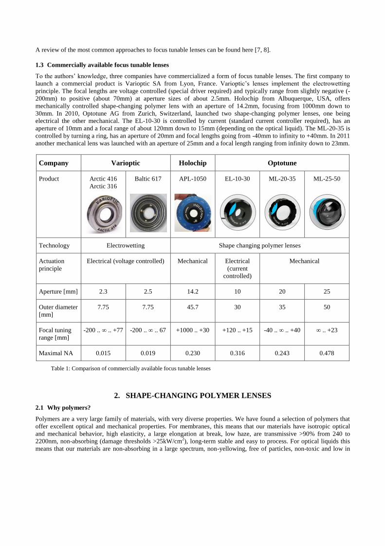
1.3 Commercially available focus tunable lenses

To the authors’ knowledge, three companies have commercialized a form of focus tunable lenses. The first company to

launch a commercial product is Varioptic SA from Lyon, France. Varioptic’s lenses implement the electrowetting

principle. The focal lengths are voltage controlled (special driver required) and typically range from slightly negative (-

200mm) to positive (about 70mm) at aperture sizes of about 2.5mm. Holochip from Albuquerque, USA, offers

mechanically controlled shape-changing polymer lens with an aperture of 14.2mm, focusing from 1000mm down to

30mm. In 2010, Optotune AG from Zurich, Switzerland, launched two shape-changing polymer lenses, one being

electrical the other mechanical. The EL-10-30 is controlled by current (standard current controller required), has an

aperture of 10mm and a focal range of about 120mm down to 15mm (depending on the optical liquid). The ML-20-35 is

controlled by turning a ring, has an aperture of 20mm and focal lengths going from -40mm to infinity to +40mm. In 2011

another mechanical lens was launched with an aperture of 25mm and a focal length ranging from infinity down to 23mm.

Company Varioptic Holochip Optotune

Product Arctic 416

Arctic 316

Baltic 617

APL-1050

EL-10-30

ML-20-35

ML-25-50

Technology Electrowetting Shape changing polymer lenses

Actuation

principle

Electrical (voltage controlled) Mechanical Electrical

(current

controlled)

Mechanical

Aperture [mm] 2.3 2.5 14.2 10 20 25

Outer diameter

[mm]

7.75 7.75 45.7 30 35 50

Focal tuning

range [mm]

-200 .. ∞ .. +77 -200 .. ∞ .. 67 +1000 .. +30 +120 .. +15 -40 .. ∞ .. +40 ∞ .. +23

Maximal NA 0.015 0.019 0.230 0.316 0.243 0.478

Table 1: Comparison of commercially available focus tunable lenses

2. SHAPE-CHANGING POLYMER LENSES

2.1 Why polymers?

Polymers are a very large family of materials, with very diverse properties. We have found a selection of polymers that

offer excellent optical and mechanical properties. For membranes, this means that our materials have isotropic optical

and mechanical behavior, high elasticity, a large elongation at break, low haze, are transmissive >90% from 240 to

2200nm, non-absorbing (damage thresholds >25kW/cm2), long-term stable and easy to process. For optical liquids this

means that our materials are non-absorbing in a large spectrum, non-yellowing, free of particles, non-toxic and low in

viscosity over a large temperature range. We present three liquids with different optical properties (see Table 2). While

the high refraction liquid with an nD of 1.56 allows for applications with very large focal tuning ranges, it is suboptimal

for polychromatic imaging due to its high dispersion characteristic. The low dispersion liquid on the other hand only has

an nD of 1.30 but an extremely high Abbe number making it the ideal choice for imaging applications.

High refraction

liquid

Medium refraction

liquid

Low dispersion

liquid

Refractive index nD 1.56 1.46 1.30

Abbe number V 31 55 100

Transmission range [nm] 330-1550 300-2000 240-2500

Toxicity None None None

Yellowing None None None

Applications Monochromatic

applications that

require a large tuning

range (e.g. lasers)

Illumination systems

based on lasers or

LEDs

Polychromatic imaging

Table 2: Comparison of three optical liquids

2.2 Shape-changing polymer lens principle

The basic principle of the presented shape-changing polymer lenses is as follows: A thin membrane builds the interface

between two chambers each containing an optically clear material, with different refractive index (Figure 1). In the

simplest case, one chamber is filled with a liquid, the other with air. The pressure difference between the two chambers

defines the deflection of the membrane and with that the radius or the lens.

Figure 1: Basic principle of the shape changing polymer lens

The pressure difference can be controlled in many ways: mechanically (e.g. by using a thread ring to push a ring-shaped

actuator down onto the chamber, see Figure 2), electromechanically (by using voice coils, piezo or stepper motors to

exert the mechanical force, see Figure 3), pneumatically (by pumping liquid into or out of the chamber) or

electrostatically (by using the principle of electroactive polymers [9, 10] to change the tension in the membrane).

n1 n2

MembraneCover glass Cover glass

p1 p2

Chamber 2Chamber 1

Figure 2: Working principle of the Optotune’s ML-20-35, which achieves a lens shape ranging from concave to flat to convex.

The ring that forms the lens is pushed towards the container, thus filling the lens with liquid.

Figure 3: Working principle of the Optotune’s EL-10-30. In this case, the lens-shaper ring remains in place relative to the

container. The only movement is a ring that pushes down on the membrane with increasing current in the outer part of the lens,

thus pumping the liquid into the lens that forms in the center.

This two chamber principle offers many possibilities. Various materials can be used to achieve the desired optical effect.

Even a double fluid lens is feasible. The tunable lenses can be shaped from convex to flat to concave and can easily be

combined with various types of cover glasses or rigid offset lenses. Figure 2 shows different configurations that are

possible.

Figure 4: Possible variations of the shape-changing polymer lens

Positive

only lens

Negative

only lens

Pos. & neg.

lens

Lens with neg.

cover glass

Lens with pos.

cover glass

Lens with higher-

order cover glass

Cover glass variationsDouble fluid lenses

n1 n2

From a number of wavefront and surface measurements, we have found that the lens shape is principally spherical. By

changing the mechanical properties of the membrane it is even possible to achieve aspheric lens shapes. Furthermore, by

using e.g. a rectangular design, a cylindrical lens can be implemented. In optical simulations the membrane can be

modeled as a single surface element, as its influence is negligible due to its minimal and homogenous thickness and the

fact that its refractive index is similar to most liquids used.

In general, lens aperture and thickness can be varied from sub‐millimeters to several centimeters. The focal tuning range

can be designed according to application requirements. However, there is always a trade-off between size, tuning range

and response time.

2.3 Pros and Cons of shape-changing polymer lenses

The biggest advantage of shape-changing polymer lenses is the additional degree of freedom offered to optics designers

by the focus tunability of the lens. A change in lens radius of several micrometers can have the same optical effect as

moving the entire lens several centimeters. Optical systems can thus be designed more compact, oftentimes with less

lenses and usually with less or no translational movement. This means that there is no more need for expensive

mechanical actuators. Less movement also leads to a more robust design, which can be completely closed so that no dust

can enter. Furthermore, the materials employed are all lighter than glass, saving overall weight. Less movement and

weight also means less power consumption and that the response time of systems with tunable lenses can be very low, in

the order of milliseconds. As can be seen in section 3.1 on auto-focus, using the radius as a degree of freedom can also

mean superior optical quality by design. Another advantage becomes obvious during production. The fact that less

optical parts are moved combined with the tunability of the radius during operation results in higher yield rates. Finally,

the components of the lens can be manufactured at low cost, making this technology suitable for consumer applications.

Some typical downsides of most focus tunable lenses remain. The coma, which is observed with electrowetting liquid

lenses, is also an issue for the approach with polymer lenses. While the effect of gravity is negligible when the lens is in

horizontal position (optical axis vertical), it is significant when used in upright position (optical axis horizontal). In

comparison to the liquid lens the coma is not temperature dependant and is typically smaller, as the membrane has a

relatively strong retaining force. Its magnitude depends mostly on size of the lens and mechanical properties of the

membrane, but also on density difference of the two materials used. With small lenses of up to 4mm aperture the coma is

negligible. At 10mm aperture, the coma term measured is in the range of 0.1 to 0.8 λ RMS (at 525nm), depending on the

membrane and liquid used. In general the quality can be improved by using stiffer and thicker membranes. However, that

does have a negative impact on tuning range or power consumption. For large lenses (greater than 10mm), best optical

quality is achieved by combining stiff membranes with the double-fluid concept, although this is at the expense of focal

tuning range.

Depending on the materials used, a thermal expansion can be observed, which has an influence on the lens radius. This

can be an issue in open loop systems. As this effect is systematic, it is consistent over the life-time of a lens and can

usually be handled by sensing the temperature and using look-up tables.

3. COMPACT OPTICAL DESIGN SOLUTIONS

In this section the advantages of focus tunable lenses are discussed from an optical design perspective. Instead of

presenting complex multi-lens designs we demonstrate some key principles that are easy to understand and replicate.

3.1 Auto-focus

Traditionally, focusing on objects at different distances is solved by moving a single lens or a group of lenses along the

optical axis. A simple example where this is done with one lens is shown in Figure 5. In A) the system is focused at

infinity and exhibits a relatively good resolution with an MTF30 value of 96 line pairs per millimeter. In B) the object

distance is reduced to 100mm and no re-focusing is performed. The result is a disastrous drop in resolution. In C) the

lens is axially repositioned by 1.36mm to re-focus, resulting in an MTF30 of 38lp/mm, which is still a large drop in

resolution. In D) the re-focusing is achieved by tuning the shape of the lens (central deflection is increased by 0.04mm).

The resulting MTF looks much better with the MTF30 at 62lp/mm.

Apart from the better resolution it can be noted that the movement for tuning the lens in D) is 34 times smaller than the

axial repositioning in C). In consequence it is reasonable to assume that an autofocus system with tunable lenses can be

designed with significantly less total height and that less actuation is needed. The latter also means that focusing can be

performed faster and with less power consumption.

Another benefit of tunable lenses becomes apparent in E). If the object distance is further decreased down to 50mm, the

system can easily be re-focused by deflecting the lens another 0.04mm. The resulting MTF curve is still significantly

better than in C) with an MTF30 of 46lp/mm. In this example, it was actually not possible to focus on 50mm by axial

movement as the lens would have crossed the aperture stop. Focus tunable lenses are thus oftentimes the only means to

design systems with very large focus ranges.

Figure 5: Comparison of focusing by translation versus tuning of a lens. For better readability only the zero-field is illustrated in

the MTF plots, as the effect is very similar for fields on the sensor.

In microscopy axial focusing of several hundred micrometers can be achieved using focus tunable lenses. Traditionally,

this would require moving the specimen or the objective with precision piezo stages. By including focus tunable lenses

in the optical pathway, focus control becomes movement-free and faster. Optotune’s EL-10-30 has proven to be

applicable for several types of microscopy including wide-field microscopy, confocal microscopy and two-photon

microscopy [11]. An example optical setup for the latter is depicted in Figure 6.

AF - tutorial model [shifted lens].zmx

Configuration 1 of 3

Layout

05.08.2011

Total Axial Length: 15.01615 mm

0.0

0

0.1

10

0.2

20

0.3

30

0.4

40

0.5

50

0.6

60

0.7

70

0.8

80

0.9

90

1.0

100

Spatial Frequency in cycles per mm

TS Diff. Limit

TS 0.0000 mm



M

o

d

u

l

u

s

o

f

t

h

e

O

T

F

Polychromatic Diffraction MTF

05.08.2011

Data for 0.5500 to 0.5500 µm.

Surface: Image



Layout

05.08.2011


0.0

0

0.1

10

0.2

20

0.3

30

0.4

40

0.5

50

0.6

60

0.7

70

0.8

80

0.9

90

1.0

100


TS Diff. Limit

TS 0.0000 mm



M

o

d

u

l

u

s

o

f

t

h

e

O

T

F


05.08.2011

Data for 0.5500 to 0.5500 µm.

Surface: Image



Layout

05.08.2011


0.0

0

0.1

10

0.2

20

0.3

30

0.4

40

0.5

50

0.6

60

0.7

70

0.8

80

0.9

90

1.0

100


TS Diff. Limit

TS 0.0000 mm



M

o

d

u

l

u

s

o

f

t

h

e

O

T

F


05.08.2011

Data for 0.5500 to 0.5500 µm.

Surface: Image

AF - tutorial model [tunable lens].zmx


Layout

05.08.2011


0.0

0

0.1

10

0.2

20

0.3

30

0.4

40

0.5

50

0.6

60

0.7

70

0.8

80

0.9

90

1.0

100


TS Diff. Limit

TS 0.0000 mm



M

o

d

u

l

u

s

o

f

t

h

e

O

T

F


05.08.2011

Data for 0.5500 to 0.5500 µm.

Surface: Image



Layout

05.08.2011


0.0

0

0.1

10

0.2

20

0.3

30

0.4

40

0.5

50

0.6

60

0.7

70

0.8

80

0.9

90

1.0

100


TS Diff. Limit

TS 0.0000 mm



M

o

d

u

l

u

s

o

f

t

h

e

O

T

F


05.08.2011

Data for 0.5500 to 0.5500 µm.

Surface: Image

B) Object at 100mmNo focus correction

A) Object at infinity

D) Object at 100mmFocusing by tuning lens (0.04mm deflection)

C) Object at 100mmFocusing by shifting lens 1.36mm

E) Object at 50mmFocusing by tuning lens (0.08mm deflection)

Figure 6: Example of axial focusing in two-photon microscopy using Optotune’s EL-10-30, a concave offset lens and 40x NA

0.8 microscope objective [12]

3.2 Optical zoom

In the previous example on auto-focus, we have seen that focus tunable lenses can significantly reduce the overall height

of an optical module. This advantage becomes even more apparent for zoom designs, where usually two or more lenses

or lens groups are axially repositioned. A very basic solution is shown in Figure 7. Two lenses are used in this example

that both change their shape from convex to concave. The backsides of the two lenses are assumed to be rigid and are

used to optimize the optical performance of the module across three zoom states. This would correspond to using lens-

shaped cover glasses with a refractive index identical to the optical liquid. All lens surfaces are spherical.

The module was designed to achieve a zoom factor of 3.27 (semi-field-of-view variable from 10° to 30°). Assuming the

image sensor to be 4mm in diagonal (1/4” sensor), the total height of the model results in 14mm. That height could be

further reduced by adding additional lenses to the system and running respective optimizations.

Figure 7: Example of a compact zoom design using two focus tunable lenses. With semi-field-of-view angles going from 30° in

wide angle to 10° in tele mode, a zoom factor of 3.27 is achieved.

0μm 300μm 600μm

Microscope objectiveOlympus LUMPlanFL/IR 40x NA 0.8

Offset lens f = -100mm

Tunable lens EL-10-30

0.8 0.6 0.5NA

Focus shift

Tunable lens 1

Tunable lens 2

¼“ image sensor

SFOV: 30 SFOV: 20 SFOV: 10

14mm

4 mm

X

Y

Z X

Y

Z X

Y

Z

3.3 Variable spot sizes in illumination

Apart from imaging applications focus tunable lenses prove to be very useful for illumination purposes. As large tuning

ranges and high optical powers are required, shape-changing condenser lenses are particularly suited. A basic application

presented here is a spot light with a variable beam angle going from “flood” to “spot” mode. The design includes an

LED, secondary optics (total-internal-reflection lens), a shape-changing condenser lens and a protective cover glass (see

Figure 8). The LED and the secondary optics together define the maximum beam angle of the spotlight, which is

achieved in the planer state of the tunable lens when the light passes through without any deflections. By tuning the

condenser lens to a convex shape the light is focused to a smaller spot size.

Figure 8: Example of adaptive illumination using Optotune’s ML-25-50 Lumilens

The components used in this example are a Cree MC-E LED, a Carclo 10196 "Frosted Wide" TIR-lens and Optotune’s

ML-25-50 Lumilens. The resulting beam angles range from 45° FWHM (full width half maximum) down to 12° FWHM.

The tuning range could be even further increased if the tunable lens was to start in a concave state, which is possible but

would require a more complex mechanical design of the lens.

A change in beam angle could also be achieved by axial movement of lenses. However, there are several advantages of

the approach with a tunable lens. As the lens is not shifted away from the light source no light is lost, which results in

high optical efficiency over all tuning states. The spot quality also remains consistent over the entire tuning range, unlike

the frequent appearance of intensity rings when lenses are shifted. Also, the low-dispersion materials ensure that no color

errors occur. Finally, the optical design remains comparably compact.

While most lighting situations require a diffuse spot, it is sometimes required to have a homogenously lit up spot with a

specific delimiting shape, e.g. a trapezoid for perspective illumination of a painting in a museum. In such cases, an

intermediate mask is imaged by projection optics. The same principle applies to gobo projectors, where the mask

contains a slide e.g. of a company logo. To vary the size of such a projection zoom optics are required that include

several lenses. Again, focus tunable lenses can help reduce the size and increase the efficiency of such optics. The basic

design for such systems follows the design discussed above in section 3.2.

4. CONCLUSION

Focus tunable lens principles have been researched for a long time and some have successfully found their way into

commercial applications in the past few years, electrowetting lenses in particular. However, the range of applications is

still limited, mainly due to the constraint in aperture size to about 2.5mm. The introduction of a variety of shape-

changing polymer lenses opens up numerous new possibilities. Especially zoom applications benefit from the increase in

focal tuning range and illumination applications benefit from large aperture sizes of several centimeters. The high quality

For layout screen shots.zmx


3D Layout

Single LED with tunable lens for lighting

25.07.2011

X

Y

Z



3D Layout


25.07.2011

X

Y

Z



3D Layout


25.07.2011

X

Y

Z



3D Layout


25.07.2011

X

Y

Z

Maximal lens deflection

(65% of lens semi-diameter)

FWHM beam angle: 12

Minimal lens deflection

(0% of lens semi-diameter)

FWHM beam angle: 45

of the polymer materials used even allow to enter applications, which have been reserved for highest quality glass lenses

like high-power laser processing in UV or near infrared. In consequence, we expect focus tunable lenses to grow in

importance, especially in designs where versatility, compactness and speed matter.

ACKNOWLEDGEMENTS

We thank Fabian F. Voigt for performing extensive tests with the EL-10-30 and providing the optical layout depicted in

Figure 6.

REFERENCES

[1] U. Wittrock, editor. “Adaptive optics for industry and medicine”. Springer (2005).

[2] O. Solgaard, F. S. A. Sandejas, and D. M. Bloom. “Deformable grating optical modulator”. Opt. Lett.,

17(9):668-690 (May 1992).

[3] G. W. Gray and S. N. Kelly. “Liquid crystals for twisted nematic display devices”. J. Mater. Chem., 9(9):2037-

2050 (1999).

[4] A. Korpel. “Acoust-optics”. Academic Press, 2nd

edition, (1988).

[5] L. Saurei, J. Peseux, F. Laune and B. Berge. “Tunable liquid lens based on electrowetting technology:

principles, properties and applications”. 10th

Ann. Micro-optics Conf. (Sept. 2004).

[6] H. Ren, D. Fox, P. A. Anderson, B. Wu, and S.-T. Wu. “Tunable-focus liquid lens controlled using a servo

motor”. Optics Express, Vol. 14, No. 18 (Sept. 2006).

[7] A. Wilson, editor. “Tunable Optics”. www.vision-systems.com/articles/2010/07/Tunable_Optics.html (2010).

[8] H. Zappe, editor. “Fundamentals of Micro-Optics”. Cambridge University Press (2010).

[9] Y. Bar-Cohen, editor. “Electroactive polymer (EAP) actuators as artificial muscles”. SPIE press, 2nd

edition

(2004).

[10] T. Mirfakhrain, J. D. W. Madden, and R. H. Baughman. “Polymer artificial muscles”. Materials Today,

10(4):30-38 (April 2007).

[11] B. F. Grewe, F. F. Voigt, M. van't Hoff, F. Helmchen, “Fast two-layer two-photon imaging of neuronal cell

populations using an electrically tunable lens.” Biomedical Optics Express, Vol. 2, Issue 7, pp. 2035-2046

(2011).

[12] A. Katsuyuki, “Embodiment 1” Japanese Patent 8–292374 (Nov. 5, 1996).

http://www.vision-systems.com/articles/2010/07/Tunable_Optics.html

compact optical design solutions using focus tunable lenses compact optical design... · compact...

Documents