comp 5138 relational database management systems semester 2, 2007 lecture 10 storage and indexing

COMP 5138COMP 5138

Relational Database Relational Database

Management Systems Management Systems

Semester 2, 2007Semester 2, 2007

Lecture 10Lecture 10

Storage and IndexingStorage and Indexing

2222

L9L9Storage &Storage &

IndexingIndexing

StorageDiskBuffer managementFile organization

IndexingTree-structured IndexingHash-based Indexing

Today’s Agenda

3333


IndexingIndexing DBMS Architecture Overview

Web Forms Application Front Ends SQL Interface

Parser Plan Executor

Optimizer Operator Evaluator

File and Access Methods

Buffer Manager

Disk Space Manager

RecoveryManager

SystemCatalog

IndexFiles

DataFiles

DATABASE

DBMS

SQL Commands

QueryEvaluationEngine

TransactionManager

LockManager

Concurrency Control

today’stopic

4444


IndexingIndexing Disks and Files

DBMS stores information on (“hard”) disks.

This has major implications for DBMS design!READ: transfer data from disk to main memory (RAM).WRITE: transfer data from RAM to disk.Both are high-cost operations, relative to in-memory operations, so must be planned carefully!Indeed, overall performance is determined largely by the number of disk I/Os done

5555


IndexingIndexingWhy Not Store Everything in Main

Memory?

Main memory costs too much to be used for all the data an enterprise needs. $150 will buy you either 1GB of RAM or 320GB of disk today.

Main memory is volatile. We want data to persist between runs. (Obviously!)

6666


IndexingIndexing Storage Hierarchy

Capacity Speed Price

CPU-Cache(SRAM)

Main Memory(DRAM)

Secondary Storage(disks, Flash etc.)

Tertiary Storage(Tape, optical discs, jukeboxes)

• Problem: Access Gap between primary and secondary storage

256 KB - 16 MB

up to 16 GB

80 GB - 1 TB

unlimited

3 GB/s

5 - 60 MB/s

1 GB/s

2 - 10 MB/s

primarystorage

16c/MB

50c/GB

5c/GB

7777


IndexingIndexing Storage Hierarchy (cont’d)

primary storage: Fastest media but volatile (cache, RAM).secondary storage: next level in hierarchy, non-volatile, moderately fast access time

also called on-line storage E.g. flash memory, magnetic disks

tertiary storage: lowest level in hierarchy, non-volatile, slow access time

also called off-line storage E.g. magnetic tape, optical storage

Typical storage hierarchy:Main memory (RAM) for currently used data.Disk for the main database (secondary storage).Tapes for archiving older versions of the data (tertiary storage).

8888


IndexingIndexing Disks

Secondary storage device of choice. Main advantage over tapes: random access vs. sequential.

Data is stored and retrieved in units called disk blocks or pages.Unlike RAM, time to retrieve a disk page varies depending upon location on disk.

Therefore, relative placement of pages on disk has real impact on DBMS performance!

Trends: Disk capacity is growing rapidly, but access speed is not!

9999


IndexingIndexing Components of a Disk

The platters spin (say, 120rps).

The arm assembly is moved in or out to position a head on a desired track. Tracks under heads make a cylinder (imaginary!).

Only one head reads/writes at any one time.

Block size is a multiple of sector size (which is fixed).

block

10101010


IndexingIndexing Accessing a Disk Page

Time to access (read/write) a disk block:seek time (moving arms to position disk head on track)rotational delay (waiting for block to rotate under head)transfer time (actually moving data to/from disk surface)

Seek time and rotational delay dominate.Seek time varies from about 1 to 20msecRotational delay varies from 0 to 10msecTransfer rate is about 1msec per 4KB page

Key to lower I/O cost: reduce seek/rotation delays! Hardware vs. software solutions?

11111111


IndexingIndexing RAID

Data Array: arrangement of several disks

RAID: Redundant Arrays of Independent Disks Data striping + redundancy

Data stripingdistribute data over several disks

High capacity and high speed

the more disk,, the lower reliability e.g., a system with 100 disks, each with MTTF of 100,000 hours (approx. 11 years), will have a system MTTF of 1000 hours (approx. 41 days)

Redundancyredundant information is maintained

high reliability by storing data redundantly, so that data can be recovered even if a disk fails

12121212


IndexingIndexing Storage Access

A database file is partitioned into fixed-length storage units called blocks (also: page). Blocks are units of both storage allocation and data transfer.

Database system seeks to minimize the number of block transfers between the disk and memory.

We can reduce the number of disk accesses by keeping as many blocks as possible in main memory.

Buffer – portion of main memory available to store copies of disk blocks.

Each portion is called a buffer frame

Buffer manager – subsystem responsible for allocating buffer space in main memory.

13131313


IndexingIndexing Buffer Manager

1. If the block is already in the buffer, the address of the block in main memory is returned

2. If the block is not in the buffer,a. the buffer manager chooses

an empty frame if possible.b. if all frames are used,

replaces (throwing out) some other block

If the block that is thrown out, was modified (marked ‘dirty’), it is written back to disk.

c. Once a frame is allocated in the buffer, the buffer manager reads the block from the disk.

DBMS calls the buffer manager when it needs a block from disk.

Buffer Manager

block

Relation

frame

buffer

Also named: page

14141414


IndexingIndexing Buffer-Replacement Policies

The algorithm by which the buffer manager decides which buffer frame to choose is called buffer-replacement policy

Several policies available which decide based on age or usage of a frame

FIFO (first in, first out)LFR (least-frequently-referenced)LRU (least recently used), CLOCK, MRU, …

Very common is a least recently used (LRU) strategyreplaces the buffer frame that has not been accessed longestMost DBMS use a variant of LRU called CLOCK

Sometimes concurrency control or recovery constrains replacement

A block may be pinned (not allowed to be replaced) or at times forced to be copied to disk (but it can stay in buffer)

15151515


IndexingIndexing DBMS vs. OS File System

OS does disk space & buffer mgmt: why not leave OS to manage these tasks for the DBMS?

Differences in OS support: portability issuesSome limitations, e.g., files can’t span disks.Buffer management in DBMS requires ability to:

pin a page in buffer pool, force a page to disk (important for implementing CC & recovery),adjust replacement policy, and pre-fetch pages based on access patterns in typical DB operations.

16161616


IndexingIndexing File Organisation

File organization: Method of arranging a file of records on external storage.

The database is stored as a collection of files. Each file is a collection of records. A record is a sequence of fields.Issues:

How to put arrange the fields in a recordHow to arrange the records in a file

Remember: a goal is to get fast access to given information

17171717


IndexingIndexing Record Layout

Two approaches to structure of individual records:Fixed-length records

All records in a single file have the same size and structure Different files are used for different relations

Variable-length recordsRecord types that allow variable lengths for one or more fields.Or, storage of multiple record types in a file.

18181818


IndexingIndexing Fixed Length Records

Information about field types same for all records in a file; stored in system catalogs.

Finding i’th field does not require scan of record.

Base address (B)

L1 L2 L3 L4

F1 F2 F3 F4

Address = B+L1+L2

19191919


IndexingIndexing Variable Length Records

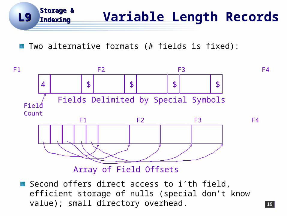
Two alternative formats (# fields is fixed):

Second offers direct access to i’th field, efficient storage of nulls (special don’t know value); small directory overhead.

4 $ $ $ $

FieldCount

Fields Delimited by Special Symbols

F1 F2 F3 F4

F1 F2 F3 F4

Array of Field Offsets

20202020


IndexingIndexing Page Formats: Fixed Length Records

Record id = <page id, slot #>. In first alternative, moving records for free space management changes rid; may not be acceptable.

Slot 1Slot 2

Slot N

. . . . . .

N M10. . .

M ... 3 2 1PACKED UNPACKED, BITMAP

Slot 1Slot 2

Slot N

FreeSpace

Slot M

11

number of records

numberof slots

21212121


IndexingIndexingPage Formats: Variable Length

Records

Can move records on page without changing rid; so, attractive for fixed-length records too.

Page iRid = (i,N)

Rid = (i,2)

Rid = (i,1)

Pointerto startof freespace

SLOT DIRECTORY

N . . . 2 120 16 24 N

# slots

22222222


IndexingIndexing Files of Records

Page or block is OK when doing I/O, but higher levels of DBMS operate on records, and files of records.FILE: A collection of pages, each containing a collection of records. Must support:

insert/delete/modify recordread a particular record (specified using record id)scan all records (possibly with some conditions on the records to be retrieved)

23232323


IndexingIndexingOrganization of Records in

Files

Heap – a record can be placed anywhere in the file where there is space

Sequential – store records in sequential order, based on the value of the search key of each record

Hashing – a hash function computed on some attribute of each record; the result specifies in which block of the file the record should be placed

Records of each relation may be stored in a separate file. In a clustering file organization records of several different relations can be stored in the same file

Motivation: store related records on the same block to minimize I/O

24242424


IndexingIndexing Heap file

Each record is inserted somewhere if there is spaceOften at the end of the file

The records are not arranged in any apparent wayThe only way to find something is to scan the whole file

Perryridge A-201 900

Brighton A-217 750

Downtown A-110 600


Downtown A-101 500

Mianus A-215 700

Redwood A-222 700

Block 1

Block 2

25252525


IndexingIndexing Sequential file

Records are kept in order based on some attributeSearch can be easier (eg binary search)But rearrangement is needed for insertion or deletion or update of the ordering attribute

Brighton A-217 750

Downtown A-110 600

Downtown A-101 500

Mianus A-215 700



Redwood A-222 700

Block 1

Block 2

Account file ordered by branch

26262626


IndexingIndexing Clustering File Organization

Simple file structure stores each relation in a separate file Can instead store several relations in one file using a clustering file organization

E.g., clustering organization of customer and depositor:

good for join queries involving depositor and customergood for queries involving one single customer and his accountsbad for queries involving only customerresults in variable size records

Customer1 record

Customer2 record

Depositor recordsRelated to customer1

Depositor recordsRelated to customer2

27272727


IndexingIndexingOracle: Logical and Physical Storage

DATABASE

OWNER

TABLESPACE

SEGMENT

DATAFILE

EXTENT

DB_BLOCK OS_BLOCK

SCHEMA

Logical Objects (Oracle) Physical Objects (O.S.)

User Objects contained in Schema - Tables, Indexes, Views, Clusters, Stored Procedures, etc

28282828


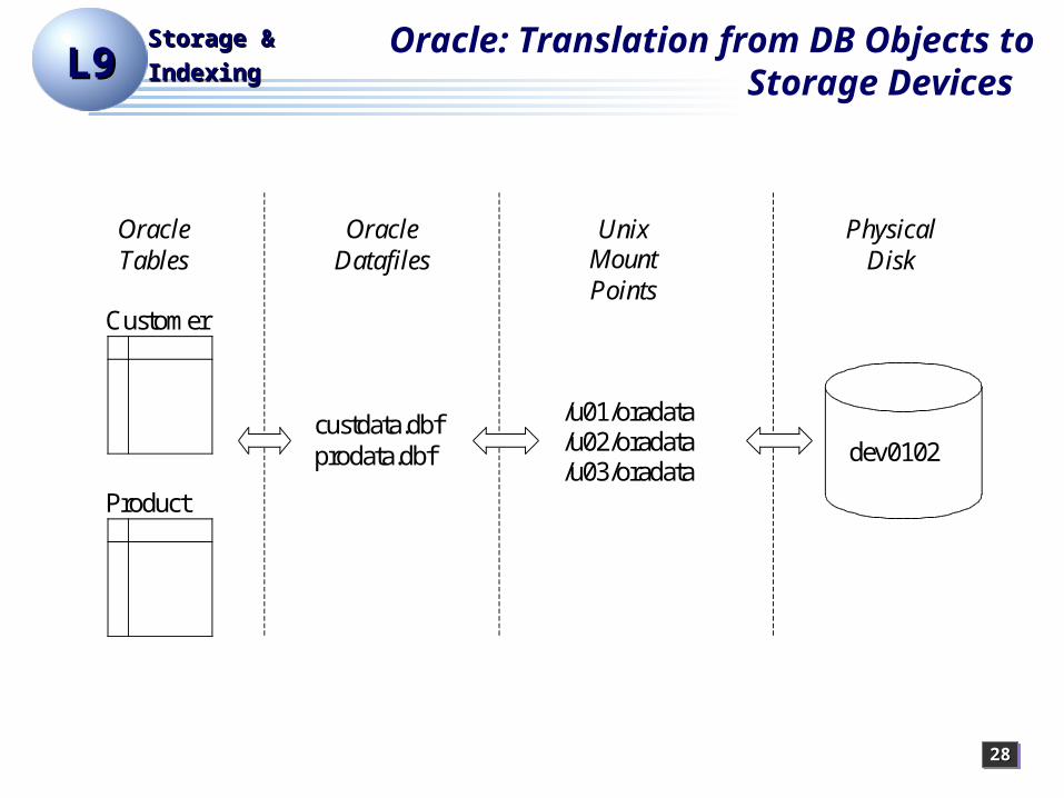
IndexingIndexing Oracle: Translation from DB Objects

to Storage Devices

Oracle Tables

Customer

Unix Mount Points

dev0102

/u01/oradata /u02/oradata /u03/oradata

custdata.dbf prodata.dbf

Product

Oracle Datafiles

Physical Disk

29292929


IndexingIndexing Data Dictionary Storage

Data dictionary (also called system catalog) stores metadata such as:

Information about relationsnames of relationsnames and types of attributes of each relationnames and definitions of viewsintegrity constraints

User and accounting information, including passwordsStatistical and descriptive data

number of tuples in each relation

Physical file organization informationHow relation is stored (sequential/hash/…)Physical location of relation

(operating system file names or disk addresses etc)

Information about indicesTypically stored as a set of relations (e.g. Oracle: USER_TABLES etc.)

30303030


IndexingIndexing

Example

attr_name rel_name type position attr_name Attribute_Cat string 1 rel_name Attribute_Cat string 2 type Attribute_Cat string 3 position Attribute_Cat integer 4 sid Students string 1 name Students string 2 login Students string 3 age Students integer 4 gpa Students real 5 fid Faculty string 1 fname Faculty string 2 sal Faculty real 3

Data Dictionary Storage

Attr_Cat(attr_name, rel_name, type, position)

31313131


IndexingIndexing



Today’s Agenda

32323232


IndexingIndexing Index Structures

An index on a relation is an access path to speed up selections on the search key fields for the index.

Any subset of the fields of a relation can be the search key for an index on the relation.Search key is not the same as primary or candidate key (minimal set of fields that uniquely identify a record in a relation).

An index consists of records (called data entries) each of which has a value for the search key eg of the form

Index files are typically much smaller than the original file

search-key pointer

33333333


IndexingIndexing Index Example

sid name birthdate

studentscountry

300697336300673435300136899 300304642 300002001 300254672

PeterHa TschiJamesNgaJesseAhmed

01.01.8431.5.7929.02.8204.05.8511.10.8630.12.80

IndiaChina

AustraliaSingapur

ChinaPakistan

AhmedHa TschiJamesJesseNgaPeter

Index(name)

Ordered index: data entries are stored in sorted order by the search key

Hash index: search keys are distributed uniformly across “buckets” using a “hash function”.

Bitmap index

34343434


IndexingIndexingAlternatives for Data Entry k*

Three alternatives for the information in the index, used to search for a value k of the search key:

Data record with value k for this attribute <k, rid of one data record with search key value k> <k, list of rids of data records with search key k>

Choice of alternative for data entries is orthogonal to the indexing technique used to locate data entries with a given key value k.

Examples of indexing techniques: B+ trees, hash-based structuresTypically, index contains auxiliary information that directs searches to the desired data entries

35353535


IndexingIndexing Alternatives for Data Entries

Alternative 1:If this is used, index structure is a file organization for data records (instead of a Heap file or sequential file).At most one index on a given collection of data records can use Alternative 1. (Otherwise, data records are duplicated, leading to redundant storage and potential inconsistency.)If data records are very large, # of pages containing data entries is high. Implies size of auxiliary information in the index is also large, typically.

36363636


IndexingIndexing Alternatives for Data Entries

Alternatives 2 and 3:Data entries typically much smaller than data records. So, better than Alternative 1 with large data records, especially if search keys are small. (Portion of index structure used to direct search, which depends on size of data entries, is much smaller than with Alternative 1.)Alternative 3 more compact than Alternative 2, but leads to variable sized data entries even if search keys are of fixed length.

37373737


IndexingIndexing Index Classification

Primary vs. secondary: If search key contains primary key, then called primary index.

Unique index: Search key contains a candidate key.

Clustered vs. unclustered: If order of data records is the same as, or `close to’, order of data entries, then called clustered index.

Alternative 1 implies clustered; in practice, clustered also implies Alternative 1 (since sorted files are rare).A file can be clustered on at most one search key.Cost of retrieving data records through index varies greatly based on whether index is clustered or not!

38383838


IndexingIndexing Clustered vs. Unclustered Index

Suppose that Alternative (2) is used for data entries To build clustered index, first sort the Heap file (with some free space on each page for future inserts). Overflow pages may be needed for inserts. (Thus, order of data recs is `close to’, but not identical to, the sort order.)

Index entries

Data entries

direct search for

(Index File)

(Data file)

Data Records

data entries

Data entries

Data Records

CLUSTERED UNCLUSTERED

39393939


IndexingIndexingUnclustered index for Heap file

Data entries in index are sorted by the search keyBut the pointers go to data records that are all over the place


Brighton A-217 750

Downtown A-110 600


Downtown A-101 500

Mianus A-215 700

Redwood A-222 700

Block 1

Block 2

A-101

A-102

A-110

A-201

A-215

A-217

A-222

Index ordered by accountno

40404040


IndexingIndexingClustered index for

Sequential file

Usually, a clustered index is sparseData entries are only used for the first data record in each data blockThis makes the index very small compared to the data

Brighton A-217 750

Downtown A-110 600

Downtown A-101 500

Mianus A-215 700



Redwood A-222 700

Account file ordered by branch, index ordered by branch

Brighton

Perryridge

41414141


IndexingIndexing Index Definition in SQL

Create an indexcreate index <index-name> on <relation-

name> (<attribute-list>)

E.g.: create index b-index on branch(branch-name)

You can use create unique index to indirectly specify and enforce the condition that the search key is a candidate key.

Not really required if SQL unique integrity constraint is supported

To drop an index drop index <index-name>

42424242


IndexingIndexingClustered Index Definition in

Oracle

Create a clustercreate cluster <clustername>

(<columnname1>, …)Columnnames are the columns used to arrange the records

Create table(s) in the clustercreate table <tablename> (column definitions as usual)cluster <clustername>

Create index on the cluster create index <index-name> on cluster <clustername>

43434343


IndexingIndexing Index structures

There are many alternatives for how to arrange the data entries in the indexAnd often there are higher levels of pointers that lead to the data entries

A tree structure for the index

Different vendors offer different choicesThis can have some impact on performanceBut the biggest performance problems usually come from not having index at all!

44444444


IndexingIndexing Tree-Structured Indices

Index Sequential Access Method (ISAM)ordered sequential file with a (fixed) primary index.Disadvantage of ISAM

performance degrades as file grows, since many overflow blocks get created. Periodic reorganization of entire file is required.

B+ Treedynamic multi-level index structuremost commonly used: B+-Treereorganization of entire file is not required to maintain performance.Disadvantages: extra insertion and deletion overhead and space overhead.

45454545


IndexingIndexing B+ Tree: Most Widely Used Index

Insert/delete at log F N cost; keep tree height-balanced. (F = fanout, N = # leaf pages)Minimum 50% occupancy (except for root). Each node contains d <= m <= 2d entries. The parameter d is called the order of the tree.Supports equality and range-searches efficiently.

Index Entries

Data Entries("Sequence set")

(Direct search)

46464646


IndexingIndexing B+-Tree Index

Non-leafPages

Pages (Sorted by search key)

Leaf

Leaf nodes contain data entries, and are chained Non-leaf nodes have index entries;only used to direct searches

P1 K1 P2 . . . Pi Ki Pi+1 . . . Pn-1 Kn-1 Pn

keys < Ki keys >= Ki

47474747


IndexingIndexing Example of a B+-tree

Note how data entries in the leaf level are sortedFind 28? 29? All > 15 and < 30?Insert/delete:

Find data entry in leaf, then change it.Need to adjust parent sometimes.

2* 3*

Root

17

30

14*16* 33*34*38*39*

135

7*5* 8* 22*24*

27

27* 29*

Entries <= 17 Entries > 17

48484848


IndexingIndexing B+-Tree Index Structure

A B+-tree is a rooted tree satisfying the following properties:

All paths from root to leaf are of the same lengthi.e., it is a balanced tree

Each node that is not a root or a leaf has between [n/2] and n (pointers to) children.

The number of pointers in a node is also called fanoutThe search keys within a node are sorted.

A leaf node has between [(n–1)/2] and n–1 valuesSpecial cases:

If the root is not a leaf, it has at least 2 children.If the root is a leaf (that is, there are no other nodes in the tree), it can have between 0 and (n–1) values.

49494949


IndexingIndexing Queries on B+-Trees

Find all records with a search-key value of k.

1. Start with the root node1. Examine the node for the smallest search-key >= k.2. If such a value exists, assume it is Ki. Then follow Pi to the child

node3. Otherwise k Kn–1, where there are n pointers in the node.

Then follow Pn to the child node.

2. Repeat the above procedure until a leaf node is reached.3. Eventually reach a leaf node. If for some i, key Ki = k follow

pointer Pi to the desired record or bucket. Else no record with search-key value k exists.

50505050


IndexingIndexing Updates on B+-Trees

To insert a data entry, when a data record is inserted (or when the search key is updated) 1. Find where the new entry should be2. If there is room in that page, insert it3. If not, split the page into two, and redistribute the entries;

then insert the new entry4. This may lead to further splits higher in the tree

The algorithm and code is complicated!Deletion can be done similarly, but in practice the entry

is simply removed, which may leave the page underfull

51515151


IndexingIndexing B+ Trees in Practice

Typical order: 100. Typical fill-factor: 67%.average fanout = 133

Typical capacities:Height 4: 1334 = 312,900,700 recordsHeight 3: 1333 = 2,352,637 records

Can often hold top levels in buffer pool:Level 1 = 1 page = 8 KbytesLevel 2 = 133 pages = 1 MbyteLevel 3 = 17,689 pages = 133 MBytes

52525252


IndexingIndexing Bulk Loading of a B+ Tree

If we have a large collection of records, and we want to create a B+ tree on some field, doing so by repeatedly inserting records is very slow.Bulk Loading can be done much more efficiently.Initialization: Sort all data entries, insert pointer to first (leaf) page in a new (root) page.

3* 4* 6* 9* 10* 11* 12* 13* 20* 22* 23* 31* 35* 36* 38* 41* 44*

Sorted pages of data entries; not yet in B+ treeRoot

53535353


IndexingIndexing Static Hashing

In a hash file organization we obtain the bucket of a

record directly from its search-key value using a hash

function.

A bucket is a unit of storage containing one or more records

(a bucket is typically a disk block).

Hash function h is a function from the set of all search-key

values K to the set of all bucket addresses B.

Hash function is used to locate records for access, insertion

as well as deletion.

Records with different search-key values may be mapped to

the same bucket; thus entire bucket has to be searched

sequentially to locate a record.

54545454


IndexingIndexingExample of Hash File

OrganizationHash file organization of account file, using branch-name as key

e.g. h(Perryridge) = 5 h(Round Hill) = 3 h(Brighton) = 3

55555555


IndexingIndexing Cost Model for Our Analysis

We ignore CPU costs, for simplicity:B: The number of data pagesR: Number of records per pageD: (Average) time to read or write disk pageMeasuring number of page I/O’s ignores gains of pre-fetching a sequence of pages; thus, even I/O cost is only approximated. Average-case analysis; based on several simplistic assumptions.

Good enough to show the overall trends!

56565656


IndexingIndexing Comparing File Organizations

Heap files (random order; insert at eof)Sorted files, sorted on <age, sal> Clustered B+ tree file, Alternative (1), search key <age, sal>Heap file with unclustered B + tree index on search key <age, sal>Heap file with unclustered hash index on search key <age, sal>

57575757


IndexingIndexing Operations to Compare

Scan: Fetch all records from diskEquality searchRange selectionInsert a recordDelete a record

58585858


IndexingIndexing Assumptions in Our Analysis

Heap Files:Equality selection on key; exactly one match.

Sorted Files:Files compacted after deletions.

Indexes: Alt (2), (3): data entry size = 10% size of record Hash: No overflow buckets.

80% page occupancy => File size = 1.25 data size

Tree: 67% occupancy (this is typical).Implies file size = 1.5 data size

59595959


IndexingIndexing Cost of Operations

(a) Scan (b) Equality (c ) Range (d) Insert (e) Delete

(1) Heap BD 0.5BD BD 2D Search +D

(2) Sorted BD Dlog 2B Dlog 2 B + # matches

Search + BD

Search +BD

(3) Clustered 1.5BD Dlog F 1.5B Dlog F 1.5B + # matches

Search + D

Search +D

(4) Unclustered Tree index

BD(R+0.15) D(1 + log F 0.15B)

Dlog F 0.15B + # matches

D(3 + log F 0.15B)

Search + 2D

(5) Unclustered Hash index

BD(R+0.125)

2D BD 4D Search + 2D

Several assumptions underlie these (rough) estimates!

60606060


IndexingIndexing Understanding the Workload

For each query in the workload:Which relations does it access?Which attributes are retrieved?Which attributes are involved in selection/join conditions? How selective are these conditions likely to be?

For each update in the workload:Which attributes are involved in selection/join conditions? How selective are these conditions likely to be?The type of update (INSERT/DELETE/UPDATE), and the attributes that are affected.

61616161


IndexingIndexing Choice of Indexes

What indexes should we create?Which relations should have indexes? What field(s) should be the search key? Should we build several indexes?

For each index, what kind of an index should it be?Clustered? Hash/tree?

62626262


IndexingIndexing Choice of Indexes (Contd.)

One approach: Consider the most important queries in turn. Consider the best plan using the current indexes, and see if a better plan is possible with an additional index. If so, create it.

Obviously, this implies that we must understand how a DBMS evaluates queries and creates query evaluation plans!For now, we discuss simple 1-table queries.

Before creating an index, must also consider the impact on updates in the workload!

Trade-off: Indexes can make queries go faster, updates slower. Require disk space, too.

63636363


IndexingIndexing Index Selection Guidelines

Attributes in WHERE clause are candidates for index keys.Exact match condition suggests hash index.Range query suggests tree index.

Clustering is especially useful for range queries; can also help on equality queries if there are many duplicates.

Multi-attribute search keys should be considered when a WHERE clause contains several conditions.

Order of attributes is important for range queries.Such indexes can sometimes enable index-only strategies for important queries.

For index-only strategies, clustering is not important!

Try to choose indexes that benefit as many queries as possible. Since only one index can be clustered per relation, choose it based on important queries that would benefit the most from clustering.

64646464


IndexingIndexing Choosing an Index

An index should support a query of the application that has a significant impact on performance

Choice based on frequency of invocation, execution time, acquired locks, table size

Example 1: SELECT E.Id FROM Employee E WHERE E.Salary < :upper AND E.Salary > :lower

– This is a range search on Salary. – Since the primary key is Id, it is likely that there is a clustered, main index on that attribute that is of no use for this query. – Choose a secondary, B+ tree index with search key Salary

65656565


IndexingIndexing Choosing An Index (cont’d)

This is an equality search on grade. Since the primary key is (sid, CourseId) it is likely that there is a main, clustered index on these attributesthat is of no use for this query.

Choose a secondary, B+ tree or hash index with search key grade

Example 2: SELECT E.sid FROM EnrolledEnrolled E WHERE E.grade = :grade

66666666


IndexingIndexing Choosing an Index (cont’d)

Equality search on StudId and grade. If the primary key is (StudId, CourseId) it is likely that there is a main, clustered index on this sequence of attributes.

If the main index is a B+ tree it can be used for this search. If the main index is a hash it cannot be used for this search. Choose B+ tree or hash with search key StudId (since grade is not as selective as StudId) or (StudId, grade)

Example 3: SELECT E.CourseCode, E.grade FROM EnrolledEnrolled E WHERE E.StudId = :sid AND E.grade = ‘D’

67676767


IndexingIndexing

Indexes with Composite Search Keys

Composite Search Keys: Search on a combination of fields.

Equality query: Every field value is equal to a constant value. E.g. wrt <sal,age> index:

age=20 and sal =75

Range query: Some field value is not a constant. E.g.:

age =20; or age=20 and sal > 10

Data entries in index sorted by search key to support range queries.

Lexicographic order, orSpatial order.

sue 13 75

bob

cal

joe 12

10

20

8011

12

name age sal

<sal, age>

<age, sal> <age>

<sal>

12,20

12,10

11,80

13,75

20,12

10,12

75,13

80,11

11

12

12

13

10

20

75

80

Data recordssorted by name

Data entries in indexsorted by <sal,age>

Data entriessorted by <sal>

Examples of composite keyindexes using lexicographic order.

68686868


IndexingIndexingComposite Search Keys

To retrieve Emp records with age=30 AND sal=4000, an index on <age,sal> would be better than an index on age or an index on sal.

Choice of index key orthogonal to clustering etc.

If condition is: 20<age<30 AND 3000<sal<5000: Clustered tree index on <age,sal> or <sal,age> is best.

If condition is: age=30 AND 3000<sal<5000: Clustered <age,sal> index much better than <sal,age> index!

Composite indexes are larger, updated more often.

69696969


IndexingIndexing

Index-Only Plans

A number of queries can be answered without retrieving any tuples from one or more of the relations involved if a suitable index is available.

SELECT D.mgrFROM Dept D, Emp EWHERE D.dno=E.dno

SELECT D.mgr, E.eidFROM Dept D, Emp EWHERE D.dno=E.dno

SELECT E.dno, COUNT(*)FROM Emp EGROUP BY E.dno

SELECT E.dno, MIN(E.sal)FROM Emp EGROUP BY E.dno

SELECT AVG(E.sal)FROM Emp EWHERE E.age=25 AND E.sal BETWEEN 3000 AND 5000

<E.dno>

<E.dno,E.eid>Tree index!

<E.dno>

<E.dno,E.sal>Tree index!

<E. age,E.sal> or<E.sal, E.age>

Tree!

70707070


IndexingIndexing

Index-Only Plans (Contd.)

Index-only plans are possible if the key is <dno,age> or we have a tree index with key <age,dno>

Which is better?What if we consider the second query?

SELECT E.dno, COUNT (*)FROM Emp EWHERE E.age=30GROUP BY E.dno

SELECT E.dno, COUNT (*)FROM Emp EWHERE E.age>30GROUP BY E.dno

71717171


IndexingIndexing Summary

Many alternative file organizations exist, each appropriate in some situation.If selection queries are frequent, sorting the file or building an index is important.

Hash-based indexes only good for equality search.Sorted files and tree-based indexes best for range search; also good for equality search. (Files rarely kept sorted in practice; B+ tree index is better.)

Index is a collection of data entries plus a way to quickly find entries with given key values.

72727272


IndexingIndexing Summary (Contd.)

Data entries can be actual data records, <key, rid> pairs, or <key, rid-list> pairs.

Choice orthogonal to indexing technique used to locate data entries with a given key value.

Can have several indexes on a given file of data records, each with a different search key.Indexes can be classified as clustered vs. unclustered, primary vs. secondary, and dense vs. sparse. Differences have important consequences for utility/performance.

73737373


IndexingIndexing Summary (Contd.)

Understanding the nature of the workload for the application, and the performance goals, is essential to developing a good design.

What are the important queries and updates? What attributes/relations are involved?

Indexes must be chosen to speed up important queries (and perhaps some updates!).

Index maintenance overhead on updates to key fields.Choose indexes that can help many queries, if possible.Build indexes to support index-only strategies.Clustering is an important decision; only one index on a given relation can be clustered!Order of fields in composite index key can be important.

74747474


IndexingIndexing Wrap-Up



75757575


IndexingIndexingExtra non-examinable

material

Details of RAID structures for disksDetails of B+-tree update operations

76767676


IndexingIndexing RAID Levels

Schemes to provide redundancy at lower cost by using disk striping combined with parity bits

Different RAID organizations, or RAID levels, have differing cost, performance and reliability characteristics

RAID Level 0: Block striping; non-redundant. Used in high-performance applications where data lost is not critical.

RAID Level 1: Mirrored disks with block striping Offers best write performance. Popular for applications such as storing log files in a database system.

RAID 0: nonredundant striping RAID 1: mirrored disks

77777777


IndexingIndexing RAID Levels (Cont.)

RAID Level 0+1: Striping and MirroringParallel reads, a write involves two disks.

RAID Level 2: Memory-Style Error-Correcting-Codes (ECC) with bit striping.

Striping unit is single bitStore code for error correcting

RAID 0+1: striping and mirroring RAID 2: error correcting codes

HDD for data storing HDD for ECC storing

78787878



RAID Level 3: Bit-Interleaved Paritya single parity bit is enough for error correction, since we know which disk has failed

When writing data, corresponding parity bits must also be computed and written to a parity bit disk

RAID Level 4: Block-Interleaved Parity; uses block-level striping, and keeps a parity block on a separate disk for corresponding blocks from N other disks.

RAID 3: bit-interleaved parity

HDD for data storing HDD for parity storing

RAID 4: block-interleaved parity

HDD for data storing HDD for parity storing

79797979



RAID Level 5: Block-Interleaved Distributed Parity; partitions data and parity among all N + 1 disks, rather than storing data in N disks and parity in 1 disk.

E.g., with 5 disks, parity block for nth set of blocks is stored on disk (n mod 5) + 1, with the data blocks stored on the other 4 disks.

RAID Level 6: P+Q Redundancy scheme; similar to Level 5, but stores extra redundant information to guard against multiple disk failures.

Better reliability than Level 5 at a higher cost; not used as widely.

RAID 5: block-interleaved distribute parity RAID 6: P+Q redundancy schem

80808080


IndexingIndexing Example of RAID Levels

RAID Level 5: Block-Interleaved Distributed Parity; partitions data and parity among all N + 1 disks, rather than storing data in N disks and parity in 1 disk.

E.g., with 5 disks, parity block for nth set of blocks is stored on disk (n mod 5) + 1, with the data blocks stored on the other 4 disks.

RAID Level 6: P+Q Redundancy scheme; similar to Level 5, but stores extra redundant information to guard against multiple disk failures.

Better reliability than Level 5 at a higher cost; not used as widely.

RAID 5: block-interleaved distribute parity RAID 6: P+Q redundancy schem

81818181


IndexingIndexing Choice of RAID Level

Factors in choosing RAID levelMonetary costPerformance: # of I/Os per second and bandwidth during normal operationPerformance during failurePerformance during rebuild of failed disk / time to rebuild failed disk

RAID 0 is used only when data safety is not important e.g. data can be recovered quickly from other sources

Level 2 and 4 never used since they are subsumed by 3 and 5Level 3 is not used anymore since bit-striping forces single block reads to access all disks, wasting disk arm movement, which block striping (level 5) avoidsLevel 6 is rarely used since levels 1 and 5 offer adequate safety for almost all applicationsSo competition is between 1 and 5 only

Level 5 is preferred for applications with low update rate,and large amounts of dataLevel 1 is preferred for all other applications

82828282


IndexingIndexingUpdates on B+-Trees:

Insertion

Find the leaf node in which the search-key value would appear.

If the search-key value is already there in the leaf node, record is added to file and if necessary a pointer is inserted.

If the search-key value is not there, then add the record to the main file if necessary. Then:

If there is room in the leaf node, insert (key-value, pointer) pair in the leaf nodeOtherwise, split the node (along with the new (key-value, pointer) entry) as discussed in the next slide.

83838383



Insertion (Cont.)

Splitting a node:take the n(search-key value, pointer) pairs (including the one being inserted) in sorted order. Place the first [ n/2] in the original node, and the rest in a new node.let the new node be p, and let k be the least key value in p. Insert (k,p) in the parent of the node being split. If the parent is full, split it and propagate the split further up.

The splitting of nodes proceeds upwards till a node that is not full is found. In the worst case the root node may be split increasing the height of the tree by 1.

84848484


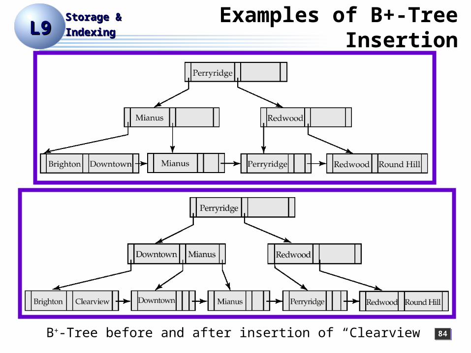
IndexingIndexingExamples of B+-Tree

Insertion

B+-Tree before and after insertion of “Clearview”

85858585



Deletion

Find the record to be deleted, and remove it from the main file

Remove (search-key value, pointer) from the leaf node

If the node has too few entries due to the removal, and the entries in the node and a sibling fit into a single node, then

Insert all the search-key values in the two nodes into a single node (the one on the left), and delete the other node.Delete the pair (Ki–1, Pi), where Pi is the pointer to the deleted node, from its parent, recursively using the above procedure.

86868686



Deletion

Otherwise, if the node has too few entries due to the removal, and the entries in the node and a sibling fit not into a single node, then

Redistribute the pointers between the node and a sibling such that both have more than the minimum number of entries.Update the corresponding search-key value in the parent of the node.

The node deletions may cascade upwards till a node which has [n/2] or more pointers is found. If the root node has only one pointer after deletion, it is deleted and the sole child becomes the root.

87878787


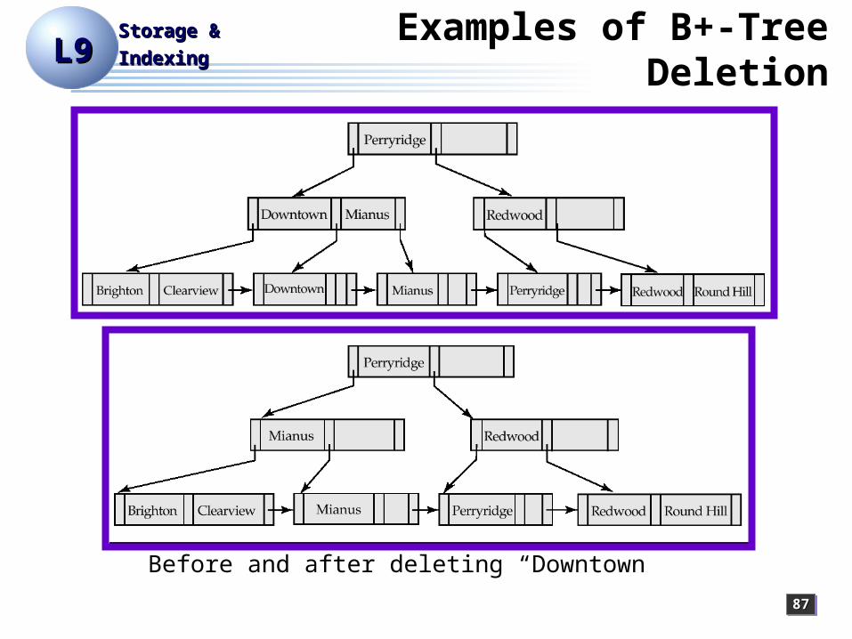
IndexingIndexingExamples of B+-Tree

Deletion

Before and after deleting “Downtown”

comp 5138 relational database management systems semester 2, 2007 lecture 10 storage and indexing

Documents