community-driven dispersal in an individual-based …grant/papers/community.pdf · community-driven...

Community-driven dispersal in an individual-basedpredator–prey model

Elise Filotas a, Martin Grant b, Lael Parrott a,*, Per Arne Rikvold c

aComplex Systems Laboratory, Departement de Geographie, Universite de Montreal, C.P. 6128, Succursale Centre-ville,

Montreal, Quebec H3C 3J7, CanadabDepartment of Physics, McGill University, 3600 rue University, Montreal, Quebec H3A 2T8, CanadacSchool of Computational Science, Center for Materials Research and Technology, National High Magnetic Field Laboratory,

and Department of Physics, Florida State University, Tallahassee, FL 32306, USA

e c o l o g i c a l c o m p l e x i t y 5 ( 2 0 0 8 ) 2 3 8 – 2 5 1

a r t i c l e i n f o

Article history:

Received 18 July 2007

Received in revised form

30 November 2007

Accepted 8 January 2008

Published on line 4 March 2008

Keywords:

Community-driven dispersal

Spatial model

Predator–prey dynamics

Individual-based modeling

Spatiotemporal patterns

a b s t r a c t

We present a spatial, individual-based predator–prey model in which dispersal is dependent

on the local community. We determine species suitability to the biotic conditions of their

local environment through a time and space varying fitness measure. Dispersal of indivi-

duals to nearby communities occurs whenever their fitness falls below a predefined

tolerance threshold. The spatiotemporal dynamics of the model is described in terms of

this threshold. We compare this dynamics with the one obtained through density-inde-

pendent dispersal and find marked differences. In the community-driven scenario, the

spatial correlations in the population density do not vary in a linear fashion as we increase

the tolerance threshold. Instead we find the system to cross different dynamical regimes as

the threshold is raised. Spatial patterns evolve from disordered, to scale-free complex

patterns, to finally becoming well-organized domains. This model therefore predicts that

natural populations, the dispersal strategies of which are likely to be influenced by their

local environment, might be subject to complex spatiotemporal dynamics.

# 2008 Elsevier B.V. All rights reserved.

avai lable at www.sc iencedi rec t .com

journal homepage: ht tp : / /www.e lsev ier .com/ locate /ecocom

1. Introduction

During the past 20 years, spatial modeling has gained

increased recognition as a theoretical tool to understand

and study spatially structured populations (Hogeweg, 1988;

Bascompte and Sole, 1995, 1998; Hanski, 1998). Interest in such

models has emerged in parallel with the desire to comprehend

how space contributes to population dynamics (Hassell et al.,

1994; Bascompte et al., 1997; Ranta et al., 1997; Bjørnstad et al.,

1999; Blasius et al., 1999) and to achieve insights into the origin

of the many spatiotemporal patterns observed in nature

(Bascompte and Sole, 1998; Marquet, 2000; Wootton, 2001).

One central mechanism in spatially explicit models is

species dispersal. Unfortunately, it has been difficult to

* Corresponding author. Tel.: +1 514 343 8032; fax: +1 514 343 8008.E-mail address: [email protected] (L. Parrott).

1476-945X/$ – see front matter # 2008 Elsevier B.V. All rights reservedoi:10.1016/j.ecocom.2008.01.002

establish regular and common rules governing species

dispersal from the numerous empirical studies of individual

movements between habitats. This absence of general

behavioral rules has often brought theoretical ecologists to

adopt the simplest possible assumptions when modeling

dispersal processes (Bowler and Benton, 2005). Most spatial

models have been designed using a density-independent rate

of dispersal, which implies that a constant ratio of the local

populations moves in each generation, regardless of local

conditions (Sole et al., 1992; Hastings, 1993; Bascompte and

Sole, 1994; Hassell et al., 1995; Rohani et al., 1996; Kean and

Barlow, 2000; Kendall et al., 2000; Sherratt, 2001). This random

or passive dispersal indeed operates on many groups of

organisms (some invertebrates, fish, insects and sessile

d.

mailto:[email protected]

http://dx.doi.org/10.1016/j.ecocom.2008.01.002

e c o l o g i c a l c o m p l e x i t y 5 ( 2 0 0 8 ) 2 3 8 – 2 5 1 239

organisms such as plants) that depend on either animal

vectors, wind or current for dispersal (Maguire, 1963; Bilton

et al., 2001; Nathan, 2006). On the other hand, it is now well

recognized that dispersal for many animals largely depends

on factors such as local population size, resource competi-

tion, habitat quality, habitat size, etc. (Johst and Brandl, 1997;

Bowler and Benton, 2005). Therefore, recent models have

started to incorporate more varied dispersal rules, and

results suggest that the dispersal mechanism can signifi-

cantly influence modeling predictions. One such dispersal

rule, which has received great attention, is the use of a

density-dependent rate of dispersal (Amarasekare, 1998,

2004; Ruxton, 1996; Doebeli and Ruxton, 1998; Sæther et al.,

1999; Ylikarjula et al., 2000). A positive rate expresses

intraspecific competition, while a negative rate mimics the

inconveniences associated with isolation, such as higher

predation risk and foraging and mating difficulties. Other

condition-dependent dispersal strategies have also been

investigated, such as dependence on habitat saturation

(South, 1999), the dependence on resource availability (Johst

and Schops, 2003), or migration following the theory of the

ideal free distribution (Ranta and Kaitala, 2000; Jackson et al.,

2004), to name but a few. For a thorough review see Bowler

and Benton (2005). These studies focus on the effect of

condition-dependent dispersal on the persistence of popula-

tions in space, as well as the stabilization and synchroniza-

tion of their dynamics.

Here, we explore the effects of a novel community-driven

dispersal strategy on the dynamics of spatially structured

predator–prey populations using an individual-based model.

We measure the impact of the community on its constituent

species using a single quantity designed to take into account

the effects of interspecific competition, intraspecific competi-

tion and resource availability on the individuals of the system.

Hence, this quantity, which we name ‘‘fitness’’, is introduced

as a way to quantify the multiple environmental pressures

arising from various biotic factors that transcend simple

population density. At this point it is important to clarify that

the term fitness as used here does not have any evolutionary

biology meaning (Ariew and Lewontin, 2004). The fitness of an

individual, as used throughout this report, should not be

confused with the usual definition of ‘‘expected number of

offspring’’. We associate the term fit with the loose definition

of a species being suited to a particular biotic environment and

hence being apt to reproduce therein.

The dispersal strategy we adopt in our model encapsulates

the idea that dispersal is a mean for individuals to enhance

their fitness. Here, the fitness of a species is a local quantity

evolving in time, which influences the reproduction rate as

well as dispersal. Individuals who are unfit to their commu-

nity, relative to a predefined fitness tolerance threshold, are

free to migrate in the ‘‘hope’’ of finding a more favorable

habitat.

We study the spatiotemporal dynamics of this predator–

prey model with respect to specific levels of tolerance through

a quantitative analysis of the spatial patterns of correlation.

We show that three distinct dynamical regimes emerge from

this community-driven dispersal model, namely random

motion, complex spatiotemporal patterns, and highly orga-

nized spatial domains. We also reveal that dynamics of such

complexity cannot be generated with the use of density-

independent motion.

2. Definition of the model

We use an individual-based model inspired by the Tangled-

Nature model (Christensen et al., 2002; Hall et al., 2002; di

Collobiano et al., 2003; Jensen, 2004) and a similar model by

Rikvold and co-authors (Rikvold and Zia, 2003; Zia and Rikvold,

2004; Sevim and Rikvold, 2005; Rikvold, 2007; Rikvold and

Sevim, 2007), which are both non-spatial models of biological

coevolution. In these models, the individuals of the commu-

nity are identified by their species genotype and interact via a

set of fixed species–species interactions. Individuals repro-

duce asexually according to their fitness and are subject to

mutation, which results in the creation of offspring of a

different genotype. The fitness of a species varies with the type

and strength of its interactions with the species of the

community, as well as their respective population sizes. As

the diversity and population sizes of species in the ecosystem

fluctuate under reproduction and mutation, so does the fitness

of each species.

Interest in such models comes from their simplicity and

impressive intermittent dynamics over long time scales,

which is reminiscent of punctuated equilibria (Eldredge and

Gould, 1972). Lawson and Jensen (2006) have investigated the

behavior of the Tangled-Nature model when coupled to a

spatial lattice under density-dependent dispersal and found

power law species–area relations over evolutionary time

scales. On the other hand, the focus of the present paper is

the dispersal dynamics of a predator–prey system. We will

therefore explore the behavior of this type of model on

ecological time scales and with the addition of spatial degrees

of freedom. To this end, we set the mutation rate to zero, and

we associate the definition of fitness used in these coevolu-

tionary models to the species reproduction probability, the

local measure of a species’ suitability to the local ecological

community. Moreover, only two species are considered, a

predator and its prey. A tacit benefit of using this framework

obviously is that it could in the future be generalized to

describe a multi-species system with mutation.

Space is modeled as a matrix composed of L � L cells, each

containing a non-spatial version of the model. Two processes

control the time development of the model: reproduction, an

intra-cell process, and dispersal, an inter-cell one. The

probability that an individual of a given species i reproduces

is given by fi, its species’ fitness, where i equals v for the prey

and p for the predator. Reproducing individuals are replaced

by two offspring, while individuals which are not able to

reproduce are removed from the ecosystem. This procedure

gives rise to non-overlapping generations. Dispersal, on the

other hand, is controlled by the parameter pmotion, which has

identical values for the predator and prey. Dispersing

individuals travel to neighboring cells. After one reproduction

and one dispersal attempt the process is reiterated. Note that

migration is the only means of interaction between cells.

Predators and prey are not allowed to feed from neighboring

cells. The local population ni(x, y, t) of species i at cell (x, y) is

therefore modified at each time iteration t, first through

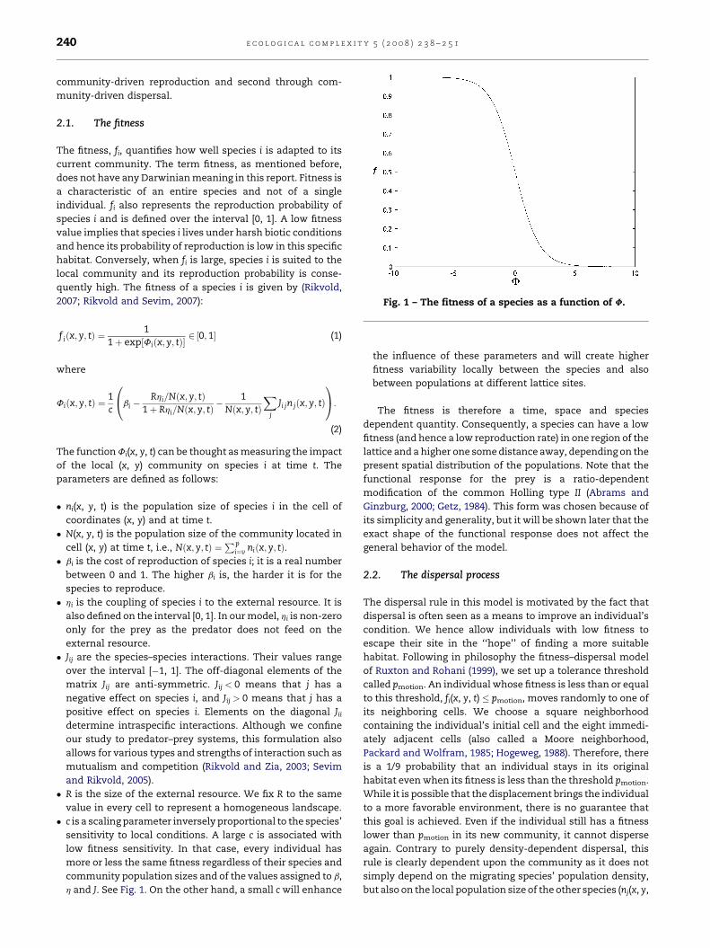
Fig. 1 – The fitness of a species as a function of F.


community-driven reproduction and second through com-

munity-driven dispersal.

2.1. The fitness

The fitness, fi, quantifies how well species i is adapted to its

current community. The term fitness, as mentioned before,

does not have any Darwinian meaning in this report. Fitness is

a characteristic of an entire species and not of a single

individual. fi also represents the reproduction probability of

species i and is defined over the interval [0, 1]. A low fitness

value implies that species i lives under harsh biotic conditions

and hence its probability of reproduction is low in this specific

habitat. Conversely, when fi is large, species i is suited to the

local community and its reproduction probability is conse-

quently high. The fitness of a species i is given by (Rikvold,

2007; Rikvold and Sevim, 2007):

f iðx; y; tÞ ¼1

1þ exp½Fiðx; y; tÞ�2 ½0; 1� (1)

where

Fiðx; y; tÞ ¼1c

bi �Rhi=Nðx; y; tÞ

1þ Rhi=Nðx; y; tÞ� 1

Nðx; y; tÞX

j

Ji jn jðx; y; tÞ

0@

1A:

(2)

The function Fi(x, y, t) can be thought as measuring the impact

of the local (x, y) community on species i at time t. The

parameters are defined as follows:

� n
i(x, y, t) is the population size of species i in the cell of
coordinates (x, y) and at time t.

� N
(x, y, t) is the population size of the community located in
cell (x, y) at time t, i.e., Nðx; y; tÞ ¼Pp

i¼v niðx; y; tÞ.
� b i is the cost of reproduction of species i; it is a real number
between 0 and 1. The higher bi is, the harder it is for the

species to reproduce.

� h
i is the coupling of species i to the external resource. It is
also defined on the interval [0, 1]. In our model, hi is non-zero

only for the prey as the predator does not feed on the

external resource.

� Ji
j are the species–species interactions. Their values range
over the interval [�1, 1]. The off-diagonal elements of the

matrix Jij are anti-symmetric. Jij < 0 means that j has a

negative effect on species i, and Jij > 0 means that j has a

positive effect on species i. Elements on the diagonal Jiidetermine intraspecific interactions. Although we confine

our study to predator–prey systems, this formulation also

allows for various types and strengths of interaction such as

mutualism and competition (Rikvold and Zia, 2003; Sevim

and Rikvold, 2005).

� R
is the size of the external resource. We fix R to the same
value in every cell to represent a homogeneous landscape.

� c
is a scaling parameter inversely proportional to the species’
sensitivity to local conditions. A large c is associated with

low fitness sensitivity. In that case, every individual has

more or less the same fitness regardless of their species and

community population sizes and of the values assigned to b,

h and J. See Fig. 1. On the other hand, a small c will enhance

the influence of these parameters and will create higher

fitness variability locally between the species and also

between populations at different lattice sites.

The fitness is therefore a time, space and species

dependent quantity. Consequently, a species can have a low

fitness (and hence a low reproduction rate) in one region of the

lattice and a higher one some distance away, depending on the

present spatial distribution of the populations. Note that the

functional response for the prey is a ratio-dependent

modification of the common Holling type II (Abrams and

Ginzburg, 2000; Getz, 1984). This form was chosen because of

its simplicity and generality, but it will be shown later that the

exact shape of the functional response does not affect the

general behavior of the model.

2.2. The dispersal process

The dispersal rule in this model is motivated by the fact that

dispersal is often seen as a means to improve an individual’s

condition. We hence allow individuals with low fitness to

escape their site in the ‘‘hope’’ of finding a more suitable

habitat. Following in philosophy the fitness–dispersal model

of Ruxton and Rohani (1999), we set up a tolerance threshold

called pmotion. An individual whose fitness is less than or equal

to this threshold, fi(x, y, t) � pmotion, moves randomly to one of

its neighboring cells. We choose a square neighborhood

containing the individual’s initial cell and the eight immedi-

ately adjacent cells (also called a Moore neighborhood,

Packard and Wolfram, 1985; Hogeweg, 1988). Therefore, there

is a 1/9 probability that an individual stays in its original

habitat even when its fitness is less than the threshold pmotion.

While it is possible that the displacement brings the individual

to a more favorable environment, there is no guarantee that

this goal is achieved. Even if the individual still has a fitness

lower than pmotion in its new community, it cannot disperse

again. Contrary to purely density-dependent dispersal, this

rule is clearly dependent upon the community as it does not

simply depend on the migrating species’ population density,

but also on the local population size of the other species (nj(x, y,


t)) and on the resource availability (R). Note that while pmotion

has the same value for the predator and the prey, this does not

imply that both species share the same dispersal rate, since

the impact of the community on each species is different.

In order to appreciate how community-driven motion

affects the predator–prey spatiotemporal dynamics, we

compare the model to its density-independent dispersal

version. In this classical scenario, the dispersal rule is

controlled by the probability parameter pind 2 [0, 1], which is

a constant value independent of species, time and space.

While it would seem ecologically more realistic to allow the

predator and prey species to disperse at different rates, in this

study, as it has been done elsewhere (Sole et al., 1992; Lawson

and Jensen, 2006), we use a single parameter pind for both

species. This simplistic set-up permits a more direct compar-

ison with the community-driven dispersal scenario. There-

fore, this means that during each iteration of the model, each

individual of both species located anywhere on the landscape

has the same probability pind to undergo dispersal, regardless

of its fitness in the local community.

Therefore, for both models, the temporal dynamics of the

local population ni(x, y, t) of species i at cell (x, y) is determined

first by the community-driven reproduction process, where

individuals are removed from the community and replaced or

not by two offspring according to the fitness of their species,

and second by the dispersal process, which controls the

migration flow in and out of cell (x, y).

3. Methods

3.1. Simulation details

The spatiotemporal dynamics of the model is investigated as a

function of the dispersal parameters pmotion and pind, for the

community-driven and density-independent models, respec-

tively. The analysis is pursued by varying pmotion and pind from

their lowest to their maximum value (0–1). Because the focus

of this article is the consequence of community-driven

dispersal, we fix the other parameters of the model:

R ¼ 200 b ¼0:3

0:5

� �h ¼

0:5

0:0

� �J ¼

�0:1 �0:9

0:9 �0:1

� �

(3)

where the first coordinate corresponds to prey attributes v

while the second coordinate is for the predator p. The

parameters are chosen so as to generate an oscillatory pre-

dator–prey dynamics, but other selections could have been

considered. Notice that we have selected a smaller cost of

reproduction for the prey (bv ¼ 0:3) as generally prey has

smaller body size than their predator and hence require less

energy to reproduce. Moreover, we have set the predator–prey

interaction to a high value (jJv pj ¼ jJ pvj ¼ 0:9) to clearly express

the negative impact of the predator on the prey and the

converse positive impact of the prey on the predator.

We are also interested in the effect of the scaling parameter

c on the spatiotemporal dynamics of the system. The majority

of our study is performed with c fixed to 0.06, a choice based on

the following ecological considerations. First, we require the

fitness of a single prey individual in the absence of predators to

be near unity and, second, the fitness of a single predator

individual in the absence of preys should be near zero. While

any c smaller than 0.06 satisfies these two conditions, such

values inconveniently produce a fitness which changes

abruptly under small modifications of the population sizes.

Indeed, due to the shape of the fitness curve as a function of F

(Fig. 1), smaller values of c generate fitness values that are

mainly distributed on the top (fitness close to one) and bottom

(fitness close to zero) branches of the curve with few

intermediate fitness values between zero and one. On the

other hand, with the intermediate value c = 0.06, the fitness of

both species has a realistic sensitivity and can cover the entire

range [0, 1], offering enough variation to generate a rich and

diverse dynamics. A detailed analysis of this scenario is

pursued with simulations repeated over 100 different initial

conditions. An initial condition corresponds to a random

spatial distribution of the population, where predator and prey

local populations ni(x, y, t) can take any value between 0 and

200 individuals. In addition, in order to explore how the

dynamics fluctuates under fitness sensitivity to the commu-

nity, we run a smaller number of simulations (20) with other

values of c chosen from the interval [0.01, 0.4].

The simulations are carried out on a square lattice of side

L = 128 with periodic boundary conditions. Every run lasts 2048

generations. Although the system reaches a statistically stable

state generally around 100 iterations, the results presented

throughout this article are computed on the last 1024 time

steps of the simulations.

During the simulations, we record the temporal evolution

of four variables: the average species density and the local

species density for each of the two species. The average

density ri(t) is a global measure (Eq. (4)). It is computed by

counting the population size of species i over the entire

territory and normalizing by the total number of cells, L2. The

local density Di(x, y, t), on the other hand, is computed for each

cell as the ratio of the local population size of species i

compared to the population size of the local community in

that cell (Eq. (5)):

riðtÞ ¼1

L2

XL

x¼1

XL

y¼1

niðx; y; tÞ (4)

Diðx; y; tÞ ¼niðx; y; tÞNðx; y; tÞ if Nðx; y; tÞ 6¼ 0

0 if Nðx; y; tÞ ¼ 0

8<: (5)

3.2. Spatial pattern analysis: the structure factor

Previous studies have mainly adopted tools from non-linear

dynamics, such as bifurcation graphs and Lyapunov expo-

nents, when analyzing the outcome of their spatial models

(Bascompte and Sole, 1994; Doebeli and Ruxton, 1998).

Although these methods are useful to identify the presence

of chaotic or complex regimes, they do not provide informa-

tion concerning the spatial structures and the scales of

emerging patterns. While the patterns of spatial synchrony

produced by population models have been investigated, these


analyses consisted in computing the temporal correlation

between time series of the population density at different

locations in the landscape (Ranta et al., 1997; Kendall et al.,

2000). Such analyses do not provide information about the

characteristic spatial scales of patterns on the landscape.

Moreover, many studies of models that generate interesting

complex structures provide only qualitative descriptions

(Hassell et al., 1995; Li et al., 2005). This prevents any detailed

comparison to be drawn between models varying in their

dispersal strategy.

Here we employ two-dimensional spectral analysis to

characterize the model’s spatial structure. More precisely, we

make use of the structure factor, akin to the R-spectrum, a

standard method of analysis in condensed matter physics

(Goldenfeld, 1992; Reichl, 1998) and statistical spatial ecology

(Platt and Denman, 1975; Renshaw and Ford, 1984). The

structure factor is simply the Fourier transform of the spatial

autocorrelation function. It gives information about spatial

patterns in reciprocal space instead of real space. The

structure factor can be understood as the spatial analogue

of the power spectrum of a temporal series of data. The power

spectrum retrieves the frequencies at which a process varies

in time. Similarly, the structure factor finds the wave numbers

characterizing the spatial patterns. Just as the period at which

a process repeats itself can be obtained as the inverse of the

frequency for a time series, the inverse of the wave number

gives the length scale of the spatial patterns. Therefore, the

structure factor is a convenient tool when spatial structures

have synchronous behavior. Moreover, the structure factor is

computationally more efficient than the spatial autocorrela-

tion function. Indeed, it is easily computed using the fast

Fourier transform (FFT). For a landscape of size L � L, this

algorithm necessitates only L2 log L2 operations compared to

the L4 used to obtain the spatial autocorrelation function

(Press et al., 1992). This difference is important when dealing

with large territories.

The structure factor is defined in the following way. LetDi(x,

y, t) be the density of species i at cell (x, y) and at time t. The

two-dimensional Fourier transform of this quantity is

Diðkx; ky; tÞ ¼XL

x¼1

XL

y¼1

e j2pkxðx=LÞ e j2pkyðy=LÞDiðx; y; tÞ (6)

where j is the imaginary unit. The structure factor is the

squared amplitude of Diðkx; ky; tÞ, averaged over a large num-

ber of initial conditions:

Siðkx; ky; tÞ ¼ hjDiðkx; ky; tÞj2i (7)

Because Di(x, y, t) is isotropic (i.e., patterns in our model do

not favor any specific orientation), the structure factor can be

averaged over the radial wave number k ¼ffiffiffiffiffiffiffiffiffiffiffiffiffiffiffiffik2

x þ k2y

q. Moreover,

once the initial period is over, the structure factor remains

statistically similar in time. We can thus average S over time

and write:

SiðkÞ ¼ hjDiðkÞj2i (8)

Our investigation of the spatial correlations in population

densities will hence consist in the analysis and comparison of

the structure factors calculated for each simulation under the

variation of pmotion, for community-driven dispersal, and pind,

for density-independent dispersal.

4. Spatiotemporal dynamics

4.1. Community-driven dispersal

In this section, we describe the spatiotemporal dynamics of

the model when the dispersal depends on the local commu-

nity. As will become clear in the next section, this dynamics is

markedly different from the one emerging from traditional

density-independent dispersal. The dynamics passes through

three different regimes as pmotion varies from 0 (no dispersal) to

1 (total dispersal), giving the appearance of phase transitions,

although at this point we cannot say if they are true phase

transitions or just smooth crossovers. Each of these regimes is

characterized by specific spatiotemporal patterns, going from

disordered to complex to highly organized domains, which

can be categorized distinctively by their respective structure

factors.

4.1.1. Spatial analysisWe provide here a detailed description of the three dynamical

regimes for the scenario c = 0.06 (Fig. 2a). Regime I, of

disordered patterns, corresponds to low fitness threshold

values. Only individuals with very low fitness are allowed to

disperse, and, as a consequence, few movements happen in

the landscape. This dynamics gives rise to random patterns in

the spatial population density: dispersal is not high enough to

induce correlations between the populations of neighboring

cells (Fig. 2b and c). The calculation of the structure factor

confirms this absence of spatial structure. In Fig. 2e the

structure factor plotted on a log–log scale depends only weakly

on the wave number k.

One can note however a peak of higher correlation around

k* � 0.5. This indicates that population densities have similar

values on cells at a small separation, 1/k*. This peak is caused

by the short-range interactions between the neighboring cells.

Consistently, the peak emerges at the same wave number for

every simulation in regime I and II, regardless of the value of

pmotion. We have also confirmed (not shown) that as we change

our definition of the cell’s neighborhood, for example by

enlarging it from 9 to 25 cells, the position of the peak also

varies in inverse proportion. On the other hand, the other

features of the structure factor are unchanged by the

modification of the neighborhood’s definition. Because it is

not related to the general properties of the community-driven

dispersal system, we can consider this peak to be an artifact of

the model’s construction. This peak indeed arises due to the

grid representation of the landscape, which does not exist in

natural systems. Therefore, it is a weakness of the model in

the sense that the model best describes the general properties

of the system only on large length scales (k� k*) and not on the

scale of single grid cells.

The complex regime II is associated with intermediate

fitness threshold values. Inside this regime the global

population is very well divided between local populations of

fitness below and above the threshold value. The motion of

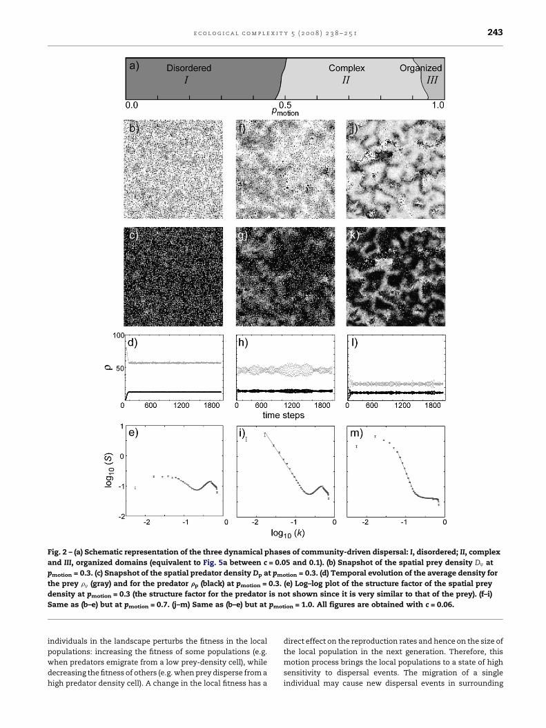
Fig. 2 – (a) Schematic representation of the three dynamical phases of community-driven dispersal: I, disordered; II, complex

and III, organized domains (equivalent to Fig. 5a between c = 0.05 and 0.1). (b) Snapshot of the spatial prey density Dv at

pmotion = 0.3. (c) Snapshot of the spatial predator density Dp at pmotion = 0.3. (d) Temporal evolution of the average density for

the prey rv (gray) and for the predator rp (black) at pmotion = 0.3. (e) Log–log plot of the structure factor of the spatial prey

density at pmotion = 0.3 (the structure factor for the predator is not shown since it is very similar to that of the prey). (f–i)

Same as (b–e) but at pmotion = 0.7. (j–m) Same as (b–e) but at pmotion = 1.0. All figures are obtained with c = 0.06.


individuals in the landscape perturbs the fitness in the local

populations: increasing the fitness of some populations (e.g.

when predators emigrate from a low prey-density cell), while

decreasing the fitness of others (e.g. when prey disperse from a

high predator density cell). A change in the local fitness has a

direct effect on the reproduction rates and hence on the size of

the local population in the next generation. Therefore, this

motion process brings the local populations to a state of high

sensitivity to dispersal events. The migration of a single

individual may cause new dispersal events in surrounding

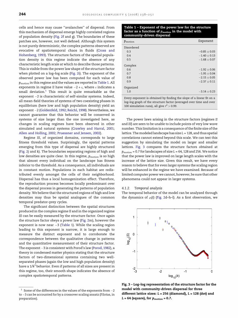
Table 1 – Exponent of the power law for the structurefactor as a function of pmotion in the model withcommunity-driven dispersal

pmotion Exponent

Disordered

0.3 �0.85 0.03

0.4 �1.40 0.13

0.5 �1.68 0.07

Complex

0.6 �1.92 0.06

0.7 �1.95 0.04

0.8 �2.15 0.05

0.9 �2.37 0.11

Organized

1.0 �3.14 0.23

Every exponent is obtained by finding the slope of a linear fit on a

log–log graph of the structure factor (averaged over time and over

100 simulation runs), all give r2 > 0.99.


cells and hence may cause ‘‘avalanches’’ of dispersal. From

this mechanism of dispersal emerge highly correlated regions

of population density (Fig. 2f and g). The boundaries of these

patches are, however, not well defined. Although this system

is not purely deterministic, the complex patterns observed are

evocative of spatiotemporal chaos in fluids (Cross and

Hohenberg, 1993). The structure factors of the spatial popula-

tion density in this regime indicate the absence of any

characteristic length scale at which to describe those patterns.

This is visible from the power law shape of the structure factor

when plotted on a log–log scale (Fig. 2i). The exponent of the

observed power law has been computed for each value of

pmotion in this regime and the values are reported in Table 1. All

exponents in regime II have value �2 + e, where e indicates a

small deviation.1 This result is quite remarkable as the

exponent �2 is characteristic of self-similar systems. Indeed,

all mean-field theories of systems of two coexisting phases in

equilibrium (here low and high population density) yield an

exponent�2 (Goldenfeld, 1992; Reichl, 1998). Nevertheless, we

cannot guarantee that this behavior will be conserved in

systems of size larger than the one investigated here, as

changes in scaling regimes have been observed in other

simulated and natural systems (Crawley and Harral, 2001;

Allen and Holling, 2002; Pruessner and Jensen, 2002).

Regime III, of organized domains, corresponds to large

fitness threshold values. Surprisingly, the spatial patterns

emerging from this type of dispersal are highly structured

(Fig. 2j and k). The boundaries separating regions of high and

low densities are quite clear. In this regime, pmotion is so high

that almost every individual on the landscape has fitness

inferior to the threshold. As a consequence, all individuals are

in constant motion. Populations in each habitat are redis-

tributed evenly amongst the cells of their neighborhood.

Dispersal has thus a local homogenization effect. Therefore,

the reproduction process becomes locally predominant over

the dispersal process in generating the patterns of population

density. We believe that the structured regions of high and low

densities may thus be spatial analogues of the common

temporal predator–prey cycles.

The significant distinction between the spatial structures

produced in the complex regime II and in the organized regime

III can be easily measured by the structure factor. Once again

the structure factor obeys a power law (Fig. 2m), however the

exponent is now near �3 (Table 1). While the scaling region

leading to this exponent is narrow, it is large enough to

measure the distinct exponent and to corroborate the

correspondence between the qualitative change in patterns

and the quantitative measurement of their structure factor.

The exponent�3 is consistent with Porod’s law (Porod, 1982), a

theory in condensed matter physics stating that the structure

factors of two-dimensional systems containing two well-

separated phases (again the low and high population density)

have a 1/k3 behavior. Even if patterns of all sizes are present in

this regime, too, their smooth shape indicates the absence of

complex spatiotemporal patterns.

1 Some of the differences in the values of the exponents from�2to�3 can be accounted for by a crossover scaling ansatz (Filotas, inpreparation).

The power laws arising in the structure factors (regimes II

and III) are seen to be unable to include points of very low wave

number. This limitation is a consequence of the finite size of the

lattice. The modeled landscape has sizeL = 128, and thus spatial

correlations cannot extend beyond this scale. We can test this

suggestion by simulating the model on larger and smaller

lattices. Fig. 3 compares the structure factors obtained at

pmotion = 0.7 for landscapes of size L = 64, 128 and 256. We notice

that the power law is improved on large length scales with the

increase of the lattice size. Given this result, we have every

reason to believe that for even larger systems the scaling region

will be enhanced in the regime we have examined. Because of

limited computer power we cannot, however, be sure that other

phenomena could not appear in larger systems.

4.1.2. Temporal analysisThe temporal behavior of the model can be analyzed through

the dynamics of ri(t) (Fig. 2d–h–l). As a first observation, we

Fig. 3 – Log–log representation of the structure factor for the

model with community-driven dispersal for three

different lattice sizes: L = 256 (diamond), L = 128 (dot) and

L = 64 (square), for pmotion = 0.7.

Fig. 4 – Standard deviation of the average population density r for the model with community-driven dispersal as a function

of pmotion for the prey (square) and for the predator (dot). Three ratio-dependent functional responses are represented: (a)

Holling type II, (b) Holling type III (sigmoidal) and (c) exponential.


note that the average density of the prey, rvðtÞ, decreases

monotonically with pmotion, while the average predator

density, rp(t), is almost constant. We suppose that this effect

arises from the fact that, for low values of pmotion, predator and

prey are mostly restricted to their original habitat giving rise to

communities of even abundance throughout the landscape.

The low predator abundance in each of these communities is

an advantage for the prey which depends on the constant

external resource for growth, and hence the prey’s average

population density stays high. As pmotion increases, predator

and prey become more mobile. The chase–escape motion

leads to regions where the prey (predator) population is

abundant and the predator (prey) population is small. In the

regions where the prey is abundant, the predator population

will tend to increase, while in the low prey abundance regions,

the predator population will be diminished. On average, these

two effects cancel out and explain the lack of change in the

predator population density with pmotion. On the other hand,

the prey are more sensitive to the predator’s presence and the

decrease of the predator population in certain regions is not

enough to compensate for the negative effect of the increase of

the predator population on the prey in the other regions.

Moreover, it is of interest to note that the temporal

dynamics of the global variable ri(t) corroborates the spatial

analysis of the dynamics. Indeed, the three-regime dynamics

we have described is also evident from the variation of the

average density ri(t) with respect to pmotion. In the disordered

regime I, the temporal evolution of ri(t) oscillates only slightly

around a mean value (Fig. 2d), while in the complex regime II,

these oscillations develop into large fluctuations (Fig. 2h).

These extreme variations can be explained by the increase of

correlation which synchronizes the oscillatory dynamics of

local populations over large areas. In the organized regime III,

domains are so well partitioned that they behave indepen-

dently. This produces out-of-phase dynamics that cancel each

other in the computation of the average density ri(t). Hence the

fluctuations of ri(t) are reduced when regime III is attained

(Fig. 2l). This statistical stabilization which reduces global

predator–prey cycles is a common phenomenon which has

been reported in other models such as the spatial Lotka–

Volterra and the spatial Rosenzweig–MacArthur model (Jan-

sen and de Roos, 2000) as well as in a spatial three-species

competition model by Durrett and Levin (1998). To gauge the

change in the amplitude of the fluctuations we show a graph of

the standard deviation of the average density, the time-

independent s(ri) (Eq. (9)), as a function of pmotion (Fig. 4a):

sðriÞ ¼ffiffiffiffiffiffiffiffiffiffiffiffiffiffiffiffiffiffiffiffiffiffiffiffihr2

i i � hrii2q

(9)

This figure shows the resemblance of this dynamics with

that of a phase transition. It should be noted, however, that for

the investigated system size, we were unable to observe the

sharp peak characteristic of a phase transition.

We have also investigated the robustness of the dynamics

against modification of the prey’s functional response. We

replaced the ratio-dependent Holling type II response (Eq. (1))

with a ratio-dependent Holling type III (sigmoid) as well as a

general ratio-dependent exponential response:

f III ¼ hiðR=Nðx; y; tÞÞ2

1þ ðR=Nðx; y; tÞÞ2(10)

fe ¼ 1� exp�hiR

Nðx; y; tÞ

� �(11)

We find that the general dynamics is unaltered under

different functional responses, but the boundaries between

the three regimes change. However, for each of these

scenarios we recover similar behavior for the standard

deviation of the average density (Fig. 4). The existence of

three different spatiotemporal regimes of dynamics is there-

fore unaffected by the foraging properties chosen for the

model.

4.1.3. Impact of the scaling parameterWe have also investigated the variation of the three regimes

with the scaling parameter c. Recall that c varies inversely with

the degree of the species sensitivity to the local biotic

conditions. It hence defines the variability in species fitness

in a community. When c is set to a large value, for example

Fig. 5 – Dynamical regimes for (a) community-driven dispersal and (b) density-independent dispersal. The phase diagrams

are expressed as functions of the level of fitness sensitivity (effect of scaling parameter c) and the dispersal probability

( pmotion in the community-driven case and pind in the density-independent case). Points drawn on the diagram have been

computed through simulations while the position of the phase boundaries has been deduced. Estimated 0.05 and 0.1 errors

on the dispersal probability should be considered in (a) and (b), respectively. As before, regime I, II and III correspond,

respectively, to the disordered, complex and organized regime.


above c = 0.4, the fitness of every species is almost identical to

0.5. Hence, the fitness of a species is not affected by its local

community and becomes independent of its position in the

landscape. Therefore, the dispersal process cannot produce

any increase or decrease of an individual’s fitness. The species

at every point on the lattice reproduce more or less at the same

rate, which precludes any spatial patterns of population

density to emerge. Thus the dynamics stays in regime I

regardless of changes in pmotion (Fig. 5a).

At the opposite end of the spectrum, a small c produces

large variations in the species’ fitness. This means that the

fitness is very sensitive to changes in the local population

sizes. Therefore, dispersal events, even of the smallest

amplitude, modify considerably the local fitness and hence

the local population density. As a result, at every pmotion this

dynamics generates complex spatial patterns and evolves in

regime II (see Fig. 5a at c = 0.01).

Fig. 5 depicts the model’s behavior with changes in pmotion

and in c. The emergence of regime II, which corresponds to

complex spatiotemporal patterns, is what distinguishes

community-driven dispersal from density-independent dis-

persal. Therefore, in an ecosystem where predators and prey

will usually have very distinct responses to their local

environment (corresponding to c in the range �(0.005, 0.1)),

we expect complex population dynamics to be one of the

possible outcomes of community-driven dispersal.

4.2. Density-independent dispersal

During dispersal controlled by a density-independent rate pind,

a fixed proportion of individuals leave each cell of the

landscape at each iteration of the model. The motion is

independent of local fitness, and, as a result, individuals that

are perfectly ‘‘happy’’ with their local biotic conditions may be

forced to move out of their habitat in an artificial manner.

Therefore, the main difference between this type of dispersal

and the previously described community-driven motion, is

that in each generation, each cell sees its population

transformed by migration flow. Every population is obliged

to participate in the dispersal process. As the dispersal

probability pind rises from 0 to 1, the participation of each

population in the dispersal process increases in a linear

fashion.

The spatial patterns produced under this dynamics are

consistent with this linear augmentation of the migration

rate (Fig. 6a). For example, consider again the case c = 0.06.

When pind is small, the interactions between the cells are

weak, and no spatial structures are apparent (Fig. 6b and c). As

pind is increased, correlations in population density are

induced by greater dispersal in the landscape, and small

and definite patterns become visible (Fig. 6f and g). As pind is

increased further, those patterns develop into highly orga-

nized domains but conserve the same explicit profile (Fig. 6j

and k). In fact, the spatial correlation increases in a smooth

manner without any abrupt modifications in the structure

factors (Fig. 6e, i, and m). Note that the cases pmotion = 1.0

(Fig. 2j–m) and pind = 1.0 (Fig. 6j–m) are statistically identical

because in both scenarios every individual continually

disperses. Accordingly, the structure factor for pind = 1.0

generates the same power law of exponent �3 as we find

for pmotion = 1.0. The exponents of the power laws for the

cases pind < 1.0 and c = 0.06 are reported in Table 2. It is seen

that the exponents increase continually from�2.5 at pind = 0.5

(as soon as patterns are noticeable) to �3 at pind = 1.0. This

dynamics is therefore equivalent to going smoothly from

regime I to regime III without passing through the spatio-

temporal complex phase.

One should note that the value of the power law exponent

is not the only factor considered when assessing the nature of

the dynamical regime as a function of dispersal. First, the

entire shape of the structure factor should be taken into

account. For example, the value of the exponents for pind = 0.3

and 0.4 is very close to �2 (Table 2), and one could be tempted

to argue that they are part of a complex regime. On the other

hand, their structure factors (not shown) have a weak k-

dependence and therefore the power law does not span as

Fig. 6 – (a) Schematic representation of the two dominant dynamical phases for density-independent dispersal: I, disordered

and III, organized domain (equivalent to Fig. 5b between c = 0.05 and 0.1). (b) Snapshot of the spatial prey density Dv at

pind = 0.1. (c) Snapshot of the spatial predator density Dp at pind = 0.1. (d) Temporal evolution of the average density for the

prey rv (gray) and for the predator rp (black) at pind = 0.1. (e) Log–log plot of the structure factor of the spatial prey density at

pind = 0.1. (f–i) Same as (b–e) but at pind = 0.7. (j–m) Same as (b–e) but at pind = 1.0. All figures are obtained at c = 0.06.


many decades as the one obtained in the presence of complex

spatiotemporal patterns. This indicates that the dynamics of

the model at pind = 0.3 and 0.4 seems to be somewhere

between a disordered state and a highly organized one, but

should not be confused with the complex phase.

Second, the absence of the complex regime also appears in

the variation of the average density ri(t) (Figs. 6d–h–l and 7).

Density-independent dispersal does not generate large fluc-

tuations of the global population size as correlations cancel

out between regions of domain organization.

Table 2 – Exponent of the power law for the structurefactor as a function of pind in the model with density-independent dispersal

pmotion Exponent

Disordered

0.1 �0.46 0.04

0.2 �1.16 0.07

0.3 �1.74 0.04

0.4 �2.13 0.10

0.5 �2.41 0.18

Organized

0.6 �2.66 0.11

0.7 �2.80 0.04

0.8 �2.99 0.04

0.9 �3.07 0.09

1.0 �3.15 0.08

Every exponent is obtained by finding the slope of a linear fit on a

log–log graph of the structure factor (averaged over time and over

100 simulation runs), all give r2 > 0.99.


Moreover, in the community-driven model, the average

prey density decreases with pmotion (Fig. 2d–h–l) while this

effect is not observed in the density-independent version

(Fig. 6d–h–l) where the prey density stays almost constant with

the variation of pind. This is another consequence of the

density-independent motion rule. Predators and prey are

allowed to move regardless of their condition in the commu-

nity, and this enhances the chance of encounters between the

two species. As a result, prey highly suited to their community,

that remained isolated from their predators in the commu-

nity-dependent case, become more vulnerable in the density-

independent counterpart, and their population density

diminishes.

The impact of the scaling parameter c on the density-

independent dispersal model is shown in Fig. 5b. For large

values of c, the dynamics remains in regime I. Spatial patterns

do not emerge in a population of poor fitness variability. For

Fig. 7 – Standard deviation of the average population

density r for the model with density-independent

dispersal as a function of pind for the prey (square) and for

the predator (dot). Note the different vertical scale from

Fig. 4.

low values of c (between 0 and 0.1) the dynamics is similar to

that described earlier for c = 0.06: a smooth transition between

a disordered state (regime I) to a highly organized state (regime

III). In the region bounded by c = 0.11 and 0.14, a narrow

complex regime emerges. We suspect that for the given values

of c, there must be a threshold in the population sizes, around

which the fitness fluctuates rapidly to values above and below

0.5. The fitness of the local populations hence becomes quite

sensitive to migration events, and as a result, regions of high

and low population densities develop in a fractal fashion

across the landscape. This complex regime is not found for

values of c below 0.11.

We should mention at this point that the boundaries

separating the regimes in the phase diagram for the density-

independent scenario (Fig. 5b) were harder to deduce than for

the community-driven model. The reason is, that the varia-

tions of the spatiotemporal patterns, and hence of the

structure factors, with dispersal probability occur gradually

in the density-independent case with no sudden changes. The

boundaries in the density-independent case could therefore

represent crossovers between different types of behavior.

There is a notable difference between the phase diagrams

of the community-driven and density-independent models

(Fig. 5). While both scenarios allow complex spatiotemporal

patterns to emerge, these two complex regimes do not develop

at the same level of fitness sensitivity. An important

distinction is that the region of high fitness sensitivity (low

c values) in the phase diagram is occupied by the complex

regime II in the community-driven case but is dominated by

the organized regime III when dispersal is density-indepen-

dent. Therefore, the density-independent model is unable to

predict self-similar complex patterns of population density at

a level of community sensitivity that we expect to find in

natural ecosystems.

5. Discussion and conclusion

In this paper, we have presented a simple spatial predator–

prey model. The model is based on a general hypothesis

regarding species interactions, foraging and reproduction. The

innovative feature of this model is that it includes the idea that

dispersal is dependent on the local community. While it is

known that dispersal is a way for individuals to escape

communities for which they are poorly adapted, to our

knowledge no spatial model so far has employed commu-

nity-driven dispersal.

We found an interesting spatiotemporal dynamics mark-

edly different from the one obtained using simple density-

independent dispersal. This difference manifests itself

through the appearance of a large complex regime, which

occurs when species are particularly sensitive to the local

environment. We expect biotic conditions in natural ecosys-

tems to indeed have a great effect on species life history, and

therefore complex population dynamics should be considered

as one of the possible outcomes of community-driven

dispersal.

The complex regime is caused by the motion rule, which

depends on a tolerance threshold, and hence brings the local

populations to a state of extreme sensitivity to dispersal


events. A single migration event may thus propagate from one

cell to another in a chain of dispersal. The resulting dynamic

phase diagram is dominated by a complex (II) and a disordered

(I) phase region, with a small organized phase region (III) for

large dispersion threshold and intermediate fitness sensitiv-

ity, as shown in Fig. 5a. This threshold-based dynamical

process cannot develop fully under density-independent

dispersal, in which case every population participates equally

in the dispersion process, irrespective of its condition in the

local community. The result is a dynamic phase diagram

dominated by the disordered (I) and organized (III) phases,

with only a very narrow complex phase region (II) for

intermediate fitness sensitivity, as shown in Fig. 5b.

Emergence of complex or chaotic spatiotemporal pat-

terns is a much discussed topic of the past decades and has

been observed in numerous spatial predator–prey models

(Segel and Jackson, 1972; Hassell et al., 1991, 1994; Sole et al.,

1992; Pascual, 1993; Wilson et al., 1993; Bascompte and Sole,

1995; Gurney et al., 1998; Savil and Hogeweg, 1999; Sherratt,

2001; Biktashev et al., 2004; Morozov et al., 2004, 2006; Li

et al., 2005). Moreover, criticality in ecosystems undergoing

phase like transition which results in the absence of

characteristic spatial scale in patterns, has been reported

in other studies (Sole and Manrubia, 1995; Malamud et al.,

1998; Kizaki and Katori, 1999; Guichard et al., 2003; Pascual

and Guichard, 2005). It is probable that self-organization is a

common phenomenon in models based on growth-inhibi-

tion or recovery-disturbance processes and does not depend

on the specific model details. On the other hand, not all

self-organized patterns are alike, and different dispersal

rules, as we have shown, can lead to different types of

emerging patterns and hence have different ecological

implications.

The conclusion of our study is therefore twofold. First, we

demonstrate the relevance of studying spatial models, in

which condition-dependent dispersal strategies are incorpo-

rated, since such dispersal strategies are common in nature

(Bowler and Benton, 2005) and are likely to cause non-trivial

dynamics. Second, we emphasize the need for comprehensive

investigations on the relation between dispersal processes

and spatial patterns. The structure factor provides significant

information about the spatial structure and the scales of

emerging patterns. We suggest that this method or similar

spatial correlation-based techniques (Bjørnstad et al., 1999;

Medvinsky et al., 2002; Morozov et al., 2006) are necessary for

detailed comparison to be drawn between models varying in

their dispersal strategy.

Acknowledgments

Funding for this research was provided by the Natural

Sciences and Engineering Research Council of Canada (NSERC)

and le Fond Quebecois de la Recherche sur la Nature et les

Technologies. We are thankful to the Reseau Quebecois de

Calcul de Haute Performance (RQCHP) for providing computa-

tional resources. Work at Florida State University was

supported in part by U.S. National Science Foundation Grant

Nos. DMR-0240078 and DMR-0444051. E. Filotas would like to

thank V. Tabard-Cossa for his help on figure editing.

r e f e r e n c e s

Abrams, P.A., Ginzburg, L.R., 2000. The nature of predation: preydependent, ratio dependent or neither? Trends Ecol. Evol.15, 337–341.

Allen, C.R., Holling, C.S., 2002. Cross-scale structure and scalebreaks in ecosystems and other complex systems.Ecosystems 5, 315–318.

Amarasekare, P., 1998. Interactions between local dynamics anddispersal: insights form single species models. Theor. Pop.Biol. 53, 44–59.

Amarasekare, P., 2004. The role of density-dependent dispersalin source-sink dynamics. J. Theor. Biol. 226, 159–168.

Ariew, A., Lewontin, R.C., 2004. The confusions of fitness. Brit. J.Philos. Sci. 55, 347–363.

Bascompte, J., Sole, R.V., 1994. Spatially induced bifurcations insingle-species population dynamics. J. Anim. Ecol. 63, 256–264.

Bascompte, J., Sole, R.V., 1995. Rethinking complexity:modelling spatiotemporal dynamics in ecology. TrendsEcol. Evol. 9, 361–366.

Bascompte, J., Sole, R.V., 1998. Spatiotemporal patterns innature. Trends Ecol. Evol. 13, 173.

Bascompte, J., Sole, R.V., Martinez, N., 1997. Population cyclesand spatial patterns in snowshoe hares: an individual-oriented simulation. J. Theor. Biol. 187, 213–222.

Biktashev, V.N., Brindley, J., Holden, A.V., Tsyganov, M.A., 2004.Pursuit-evasion predator–prey waves in two spatialdimensions. Chaos 14, 988–994.

Bilton, D.T., Freeland, J.R., Okamura, B., 2001. Dispersal infreshwater invertebrates. Annu. Rev. Ecol. Syst. 32, 159–181.

Bjørnstad, O.N., Ims, R.A., Lambin, X., 1999. Spatial populationdynamics: analyzing patterns and processes of populationsynchrony. Trends Ecol. Evol. 14, 427–432.

Blasius, B., Huppert, A., Stone, L., 1999. Complex dynamics andphase synchronization in spatially extended ecologicalsystems. Nature 399, 354–359.

Bowler, D.E., Benton, T.G., 2005. Causes and consequences ofanimal dispersal strategies: relating individual behavior tospatial dynamics. Biol. Rev. 80, 205–225.

Christensen, K., di Collobiano, S.A., Hall, M., Jensen, H.J., 2002.Tangled nature: a model of evolutionary ecology. J. Theor.Biol. 216, 73–84.

Crawley, M.J., Harral, J.E., 2001. Scale dependence in plantbiodiversity. Science 291, 864–868.

Cross, M.C., Hohenberg, P.C., 1993. Pattern formation outside ofequilibrium. Rev. Mod. Phys. 65, 851–1112.

di Collobiano, S.A., Christensen, K., Jensen, H.J., 2003. Thetangled-nature model as an evolving quasi-species model. J.Phys. A: Math. Gen. 36, 883–891.

Doebeli, M., Ruxton, D.G., 1998. Stabilization through spatialpattern formation in metapopulations with long-rangedispersal. Proc. R. Soc. Lond. B 265, 1325–1332.

Durrett, R., Levin, S., 1998. Spatial aspects of interspecificcompetition. Theor. Pop. Biol. 53, 30–43.

Eldredge, N., Gould, S.J., 1972. Punctuated equilibria: analternative to phyletic gradualism. In: Schopf, T.J.M. (Ed.),Models in Paleobiology. Freeman, Cooper & Company, SanFrancisco, pp. 82–115.

Getz, W.M., 1984. Population dynamics: a resource per capitaapproach. J. Theor. Biol. 108, 623–644.

Goldenfeld, N., 1992. Lectures on Phase Transitions and theRenormalization Group. Addison-Wesley, Boston.

Guichard, F., Halpin, P.M., Allison, G.W., Lubchenco, J., Menge,B.A., 2003. Mussel disturbance dynamics: signatures ofoceanographic forcing from local interactions. Am. Nat. 161,889–904.


Gurney, W.S.C., Veitch, A.R., Cruickshank, I., McGeachin, G.,1998. Circles and spirals: population persistence in aspatially explicit predator–prey model. Ecology 79, 2516–2530.

Hall, M., Christensen, K., di Collobiano, S.A., Jensen, H.J., 2002.Time-dependent extinction rate and species abundance in atangled-nature model of biological evolution. Phys. Rev. E66, 011904.

Hanski, I., 1998. Metapopulation dynamics. Nature 396, 41–49.Hassell, M.P., Comins, H.N., May, R.M., 1991. Spatial structure

and chaos in insect population dynamics. Nature 353, 255–258.

Hassell, M.P., Comins, H.N., May, R.M., 1994. Species coexistenceand self-organizing spatial dynamics. Nature 370, 290–292.

Hassell, M.P., Miramontes, O., Rohani, P., May, R.M., 1995.Appropriate formulations for dispersal in spatiallystructured models: comments on Bascompte & Sole. J.Anim. Ecol. 64, 662–664.

Hastings, A., 1993. Complex interactions between dispersal anddynamics: lessons from coupled logistic equations. Ecology74, 1362–1372.

Hogeweg, P., 1988. Cellular automata as a paradigm forecological modeling. Appl. Math. Comput. 27, 81–100.

Jackson, A.L., Ranta, E., Lundberg, P., Kaitala, V., Ruxton, D.G.,2004. Consumer–resource matching in a food chain whenboth predators and prey are free to move. Oikos 106, 445–450.

Jansen, V.A.A., de Roos, A.M., 2000. The role of space in reducingpredator–prey cycles. In: Dieckmann, U., Law, R., Metz, J.A.J.(Eds.), The Geometry of Ecological Interactions. CambridgeUniversity Press, Cambridge, pp. 183–201.

Jensen, H.J., 2004. Emergence of species and punctuatedequilibrium in the tangled nature model of biologicalevolution. Physica A 340, 697–704.

Johst, K., Brandl, R., 1997. The effect of dispersal on localpopulation dynamics. Ecol. Model. 104, 87–101.

Johst, K., Schops, K., 2003. Persistence and conservation of aconsumer–resource metapopulation with localoverexploitation of resources. Biol. Cons. 109, 57–65.

Kean, J.M., Barlow, N.D., 2000. The effects of density-dependence and local dispersal in individual-basedstochastic metapopulations. Oikos 88, 282–290.

Kendall, B.E., Bjørnstad, O.N., Bascompte, J., Keitt, T.H., Fagan,W.F., 2000. Dispersal, environmental correlation, andspatial synchrony in population dynamics. Am. Nat. 155,628–636.

Kizaki, S., Katori, M., 1999. Analysis of canopy-gap structures offorests by Ising–Gibbs states—equilibrium and scalingproperties of real forests. J. Phys. Soc. Jpn. 68, 2553–2560.

Lawson, D., Jensen, H.J., 2006. The species–area relationship andevolution. J. Theor. Biol. 241, 590–600.

Li, Z.-Z., Gao, M., Hui, C., Han, X.-Z., Shi, H., 2005. Impact ofpredator prey pursuit and prey evasion on synchrony andspatial patterns in metapopulation. Ecol. Model. 185, 245–254.

Maguire Jr., B., 1963. The passive dispersal of small aquaticorganisms and their colonization of isolated bodies ofwater. Ecol. Monogr. 33, 161–185.

Malamud, B.D., Morein, G., Turcotte, D.L., 1998. Forest-fires: anexample of self-organized critical behavior. Science 281,1840–1842.

Marquet, P.A., 2000. Invariants, scaling laws, and ecologicalcomplexity. Science 289, 1487–1488.

Medvinsky, A.B., Petrovskii, S., Tikhonova, I.A., Molchow, H., Li,B.-L., 2002. Spatiotemporal complexity of plankton and fishdynamics. SIAM Rev. 44, 311–370.

Morozov, A., Petrovskii, S., Li, B.-L., 2004. Bifurcations and chaosin a predator–prey system with Allee effect. Proc. R. Soc.Lond. B 271, 1407–1414.

Morozov, A., Petrovskii, S., Li, B.-L., 2006. Spatiotemporalcomplexity of patchy invasion in a predator–prey systemwith Allee effect. J. Theor. Biol. 238, 18–35.

Nathan, R., 2006. Long-distance dispersal of plants. Science 313,786–788.

Packard, N.H., Wolfram, S., 1985. Two-dimensional cellularautomata. J. Stat. Phys. 38, 901–946.

Pascual, M., 1993. Diffusion-induced chaos in spatial predator–prey system. Proc. R. Soc. Lond. B 251, 1–7.

Pascual, M., Guichard, F., 2005. Criticality and disturbancein spatial ecological systems. Trends Ecol. Evol. 20,88–95.

Platt, T., Denman, K.L., 1975. Spectral analysis in ecology. Annu.Rev. Ecol. Syst. 6, 189–210.

Porod, G., 1982. General theory. In: Glatter, O., Kratky, L. (Eds.),Small Angle X-ray Scattering. Academic Press, New York,pp. 17–51.

Press, W.H., Flannery, B.P., Teukolsky, S.A., Vetterling, W.T.,1992. Numerical Recipes in C: The Art of ScientificComputing, 2nd ed. Cambridge University Press, New York.

Pruessner, G., Jensen, H.J., 2002. Broken scaling in the forest firemodel. Phys. Rev. E 65, 056707.

Ranta, E., Kaitala, V., 2000. Resource matching and populationdynamics in a two-patch system. Oikos 91, 507–511.

Ranta, E., Kaitala, V., Lundberg, P., 1997. The spatial dimensionin population fluctuations. Science 278, 1621–1623.

Reichl, L.E., 1998. A Modern Course in Statistical Physics, 2nded. Wiley & Sons, New York.

Renshaw, E., Ford, E.D., 1984. The description of spatial patternsusing two-dimensional spectral analysis. Vegetatio 56, 75–85.

Rikvold, P.A., 2007. Self-optimization, community stability, andfluctuations in two individual-based models of biologicalcoevolution. J. Math. Biol. 55, 653–677.

Rikvold, P.A., Sevim, V., 2007. An individual-based predator–prey model for biological coevolution: fluctuations, stability,and community structure. Phys. Rev. E 75, 051920.

Rikvold, P.A., Zia, R.K.P., 2003. Punctuated equilibria and 1/fnoise in a biological coevolution model with individual-based dynamics. Phys. Rev. E 68, 031913.

Rohani, P., May, R.M., Hassell, M.P., 1996. Metapopulations andequilibrium stability: the effects of spatial structure. J.Theor. Biol. 181, 97–109.

Ruxton, D.G., 1996. Density-dependent migration and stabilityin a system of linked populations. Bull. Math. Biol. 58, 643–660.

Ruxton, D.G., Rohani, P., 1999. Fitness-dependent dispersal inmetapopulations and its consequences for persistence andsynchrony. J. Anim. Ecol. 68, 530–539.

Sæther, B.-E., Engen, S., Russell, L., 1999. Finite metapopulationmodels with density-dependent migration and stochasticlocal dynamics. Proc. R. Soc. Lond. B 266, 113–118.

Savil, N.J., Hogeweg, P., 1999. Competition and dispersal inpredator–prey waves. Theor. Pop. Biol. 56, 243–263.

Segel, L.A., Jackson, J.L., 1972. Dissipative structure: anexplanation and an ecological example. J. Theor. Biol. 37,545–559.

Sevim, V., Rikvold, P.A., 2005. Effects of correlated interactionsin a biological coevolution model with individual-baseddynamics. J. Phys. A: Math. Gen. 38, 9475–9489.

Sherratt, J.A., 2001. Periodic travelling waves in cyclic predator–prey systems. Ecol. Lett. 4, 30–37.

Sole, R.V., Manrubia, S.C., 1995. Are rainforests self-organized ina critical state? J. Theor. Biol. 173, 31–40.

Sole, R.V., Bascompte, J., Valls, J., 1992. Stability and complexityof spatially extended two-species competition. J. Theor.Biol. 159, 469–480.

South, A., 1999. Dispersal in spatially explicit populationmodels. Conserv. Biol. 13, 1039–1046.


Wilson, W.G., de Roos, A.M., McCauley, E., 1993. Spatialinstabilities within the diffusive Lotka–Volterra system: indi-vidual-based simulation results. Theor. Pop. Biol. 43, 91–127.

Wootton, J.T., 2001. Local interactions predict large-scalepattern in empirically derived cellular automata. Nature413, 841–844.

Ylikarjula, J., Alaja, S., Laakso, J., Tesar, D., 2000. Effects of patchnumber and dispersal patterns on population dynamics andsynchrony. J. Theor. Biol. 207, 377–387.

Zia, R.K.P., Rikvold, P.A., 2004. Fluctuations and correlations inan individual-based model of biological coevolution. J. Phys.A: Math. Gen. 37, 5135–5155.

community-driven dispersal in an individual-based …grant/papers/community.pdf · community-driven...

Documents