Community-Based Stormwater Mitigation:

Rescuing a Clam Fishery in Middens Creek, N.C.

by

Stephen J. Durkee

Dr. Bill Kirby-Smith, Advisor

May 2008

Masters project submitted in partial fulfillment of the requirements for the Master of Environmental Management degree in

the Nicholas School of the Environment and Earth Sciences of Duke University

2008

Abstract

Eastern North Carolina’s expansive aquatic environment, with large lagoonal sounds tapering

into winding inland waterways, maximizes the number of residents with direct influence on our

coastal waters. Such a system creates a complex management scenario where regulating non-

point source pollution proves difficult. To examine sources and potential remedies of fecal

coliform loading, a study was initiated in our model waterway, Middens Creek, where active

shellfish harvesting is ongoing. Through a multi-phase investigation, current legislation aimed

at reducing stormwater impacts is reviewed and pre- and post-storm fecal coliform levels

characterized. It became evident during the course of the study that non-point source runoff is

the primary way fecal coliform is conveyed into Middens Creek. Quantifying the impact of this

runoff in the subwatershed was further extended to examine the statistical link between

human development and bacteria levels within the creek and significant correlations between

the two were found. Finally, public outreach and education was initiated to affect grassroots

change among the residents living along the model waterway in an effort to mitigate the trend

anthropogenic impacts.

Table of Contents:

Introduction p. 1

Phase I: Policy Review p. 4

Policy Framework p. 4

Total Ecology p. 10

Phase II: Current Fecal Coliform Characterization and Shoreline Survey p. 14

Introduction p. 14

Methods p. 14

Results p. 17

Discussion p. 18

Conclusion p. 21

Phase III: Historical/Spatial Data Analysis p. 23

Introduction p. 23

Methods p. 23

Discussion p. 27

Conclusion p. 30

Phase IV: Public Outreach and Education p. 31

Project Conclusion p. 33

References Cited p. 35

Figures p. 38

Graphs p. 49

Tables p. 57

Appendix p. 65

Introduction

Coastal North Carolina is home to the second most expansive estuarine ecosystem on

the east coast of the US, and is among the most important nursery habitats for juvenile fish

and invertebrates (Lin et al 2007). The Pamlico Sound, as it stretches south into the Core

Sound and Back Sound, is typified by a shallow sandy bottom and high salinity variability due

to fresh and saltwater inputs, precipitation and evaporation (Giese et al 1985). While regular

inputs of seawater enter the system through inlets into the Atlantic Ocean, the lagoonal

nature of the estuary limits free flow back and forth producing a moderately closed system

(Paerl et al 2001). Due to the fragile nature of the resource and the economic importance of

seafood harvesting in the area, adequate water quality is of specific concern to residents,

visitors, and policy makers in the area. Nowhere is this concern more critical than in the

coastal counties lying at the confluence of the aquatic environment and human development.

Here, the impacts of man’s presence are concentrated along the sensitive coastal areas, and

general housing data shows little sign of this trend slowing (Mallin et al 2001). In an effort to

investigate our impact on these coastal waters, a study was initiated on a typical waterway

found in Eastern North Carolina. Middens Creek, a small tidal waterway located outside

Smyrna, North Carolina, was selected as an appropriate locale for study (Figure 1). Its small

size allows for complete, timely water quality characterization, the low population density

(Carteret County Tax Office 2007) simplifies public outreach efforts, and the creek is close

enough to the testing laboratory at the Duke University Marine Laboratory (DUML) to allow for

quick response in the collection of post-storm samples. Furthermore, the waterway contains

1

several actively harvested shellfish leases giving a quantifiable economic consequence to

degraded water quality.

Since shellfishing is one of the major uses of the creek, water quality sampling focused

on fecal coliform (FC) levels within the waterway. Fecal coliform is an enteric bacteria found in

the digestive tract of all warm blooded animals and is reported as Most Probable Number of

Colonies (MPN). Although it is not harmful to shellfish or human consumers, it is a fairly

simple bacteria to test for and is therefore used as an indicator of the presence of other, more

dangerous microbes found in endothermic gut tracts (Dadswell 1993). As shellfish take in and

filter the ambient water, harmful bacteria and viruses are inadvertently collected and stored

within their tissue. Since the shellfish are often consumed raw, these microbes pose potential

health concerns for consumers, and therefore harvest is banned when levels of the indicator

bacteria, fecal coliform, reach a certain concentration. In North Carolina the Shellfish

Sanitation Section is responsible for testing shellfishing waters for fecal coliform and making

recommendations as to their harvesting status. A section within the Division of Environmental

Health, Shellfish Sanitation will recommend a closure of a waterway when the geomean of 15

consecutive samples exceeds the 14 MPN threshold. In 2007, the closure line in Middens

Creek, which indicates that all upstream waters are closed for harvest, was moved

downstream 100 yards (DEH 2006), creeping to within a quarter mile of actively harvested

clam beds. Figure 2 shows both the old and new shellfish closure lines, as well as the

additional 5 acres of closed area. This map shows that the majority of the creek is now closed,

and that the current shellfish lease holders at the mouth of the waterway face an uncertain

2

future. This loss of productive harvesting grounds is the focus of the project, and reversing the

trend is the goal.

This project and study location is particularly timely, as the state government is

currently in the process of making changes to the coastal stormwater rules. These changes,

which have passed through a series of public comment periods and appear to be on their way

to the legislature for review, are highlighted within this study. The contentious nature of these

rules have raised interest in this project, and increased interest in the public outreach and

education efforts. As of the submission date for this project, the North Carolina Legislature

sent the coastal stormwater rules back to the Environmental Management Commission for

some minor changes is wording. No deviations from the proposal are expected, and the rules

should be resubmitted shortly. (Wynn 2007)

This study consists of four phases to ensure a well-rounded examination of shellfish

closure causes and solutions. The first phase involves a policy review examining the federal,

state, and local laws impacting water quality in the study area. The second consists of

gathering current pre and post-storm fecal coliform data and shoreline descriptions. The third

phase examines statistical links between development and bacteria levels within the

subwatershed as well as past and future development trends. Finally, the fourth phase, public

outreach and education, provides a chance to directly communicate project results to the

residents of Middens Creek in an effort to affect grassroots change.

3

Phase I: Policy Review

In the context of working toward stopping and possibly reversing the trend of

increasing shellfish closure area, the policies regulating coastal stormwater are discussed as

well as the federal mandates that spurred their development. The total ecology of the issue is

described as well, including both the biophysical and human components, to give context and

highlight the major players in the issue.

Policy Framework

The foundation of improving coastal water quality lies with the Federal Water Pollution

Control Act. More widely known as the Clean Water Act, this mandate has roots in a federal

initiative passed in 1948 that tasked the Public Health Service with reducing pollution in

interstate waterways. This original plan only supplied money to states for waterway cleanup,

and did not have any federal standards by which to mark progress or set goals (Federal Wildlife

Laws Handbook 1998). In 1972, this idea was greatly expanded and reorganized into what

came to be called the Clean Water Act (CWA). The official goal of this Act is to prevent,

reduce, and eliminate pollution in surface waters across the country (Federal Wildlife Laws

Handbook 1998). Similar to its precursor, the Act tasks the states with control of the actual

pollution reduction methods. However, the federal government took a more active role after

the expansion and reorganization. The federal level Environmental Protection Agency (EPA)

controls the implementation and enforcement of the CWA, and provides financial, technical,

and scientific support to the state agencies (Copeland 2002). In this support role, the EPA has

4

the goal of maintaining the chemical, physical and biological integrity of the nation’s waters for

the purpose of protecting and propagating fish and other aquatic species, offering safe water

for both recreational purposes as well for the public water use, and maintaining the supply for

agricultural and industrial uses. The Act also provided specific goals for water quality. These

objectives included having all of the nation’s waters clean enough for fishing and swimming by

mid-1983, and to attain a zero discharge of pollutants by 1985 (Copeland 2002). These goals

were admittedly quite ambitious and thirty-five years later we still have not reached them.

However this ambitiousness is exactly why the act made such great strides in improving water

quality nationwide.

The initial version of the Clean Water Act targeted point sources of water pollution. It

operated with the belief that any discharge of pollutants into public waterways is illegal (EPA

2007a). However, the EPA understood that some point sources would be easier to stop than

others, and some might even be necessary to maintain economic viability. To this end, the

primary enforcement tool of the CWA, the National Pollutant Discharge Elimination System

(NPDES) permits were introduced. These permits are mandatory for any point discharges into

waterways, and are administered at the state level with specific requirements varying on a

state by state basis (DWQ 2007a). Progress towards improving water quality was quite rapid

in the years following the implementation of the NPDES permit program (EPA 2005).

Regulating point source discharges ended up being fairly manageable, however it soon became

evident that the initial goals set forth by the EPA were not being met (Klimeck 2005). Despite

drastic improvements, the attainment of fishable and swimmable waterways proved difficult.

The reasons for the shortfalls were soon highlighted through emerging research regarding the

5

significance of non-point sources of pollution. These diffuse sources are generally the result of

stormwater runoff, and currently represent the most significant source of water pollution in

the country (Mallin et al 2001). Furthermore, non-point sources are quite difficult to identify

and mitigate and thereby present considerable regulatory challenges. To this end, major

amendments to the Clean Water Act were passed in 1987 to address the non-point problems

(EPA 2007b).

The 1987 amendments to the CWA, staying within the spirit of the original form of the

Act, tasked the states to develop management programs for controlling stormwater runoff

(DWQ 2007b). The framework for the state-based management was established by the EPA

and included implementation of runoff controls across two phases (Copeland 2002). While

there is no federal authority for specifically reducing non-point source discharge, states are

required to develop informative Total Maximum Daily Load (TMDL) levels for any waterways

that are impaired by nonpoint sources (EPA 2003). In North Carolina where Middens Creek is

located, the day to day activities of implementation and enforcement are carried out by the

North Carolina Department of Water Quality (DWQ). In North Carolina, each phase targets a

different scale of nonpoint sources such as stormwater conveyance systems and construction

sites. The first phase, Phase I, aims regulations toward large scale runoff contributors. These

contributors include stormwater conveyance systems, called Municipal Separate Storm Sewer

Systems (MS4s), that serve greater than 100,000 people and construction sites that disturb

more than five acres of ground. Each requires a Phase I NPDES permit and must meet all

required stipulations such as formulating a plan to reduce pollutant loading, removal of

6

pollutants that have gotten into the system, and ensuring that non-stormwater discharges are

disconnected from any MS4s (EPA 2003, Klimeck 2005).

Once North Carolina had Phase I firmly implemented, discussions began to develop

Phase II of the stormwater control program. Implemented in 2006, Phase II is essentially an

extension of the existing NPDES stormwater permitting program already in place under Phase I

plans (EPA 2005, EPA 2007d). The program requires permits for smaller nonpoint sources

including MS4s that serve less than 100,000 people but are still defined as an urbanized area

by the Bureau of the Census. Phase II permits are also required for construction sites that

disturb between one and five acres of land (DWQ 2007c). It is important to note that the

larger MS4s and construction sites are still regulated under the Phase I permitting system. The

new Phase II regulations also require a more holistic approach to pollution control, working

toward a watershed based approach rather than a source by source approach. Included within

this holistic vision is the requirement of public outreach and education to inform residents of

the impact of stormwater, and what they can do to help dampen or mitigate its effects

(Klimeck 2005).

Due to the geographic features of North Carolina, most of the coastal counties remain

remote with low population densities and low development levels. As such, most are not

subject to either Phase I or Phase II stormwater permitting. In fact, of the 20 coastal counties,

only 3 are large enough to require Phase II permits for their MS4s (DWQ 2007d). Figure 3

highlights the three impacted counties in yellow. In the face of continued water quality

degradation with no federally mandated regulations to control runoff, the North Carolina

7

Environmental Management Commission (EMC) was tasked in the late 1980s with developing

rules to control runoff near coastal waters (Rawlins 2007). Most sensitive of these coastal

waters are those open to active shellfish harvesting. This class of water, termed SA waters, is

held to the highest water quality standards due to the potential health risks associated with

shellfish consumption. This resource is often consumed raw, and therefore requires strict

regulations to keep biological contaminants from building up within its flesh (Mallin et al

2000). As discussed with Middens Creek specifically, fecal coliform is used as an indicator of

bacterial loading and is often delivered to waterways via stormwater runoff. Due to these

sensitivities and their susceptibility to stormwater runoff, special requirements were included

in the EMC’s rules pertaining to SA waters. The following are the major rules pertaining to

development lying within a half mile of SA water or directly draining to it:

- To qualify as low density development, percent impervious cover must be less than

25% of the parcel of land

- If greater than 25% impervious cover exists, and thereby designated as high density

development, engineered stormwater controls must be in place to control a 1.5”

rainfall event

- 30 foot vegetated buffer surrounding SA waters where impervious surfaces exist

- Permits required for construction disturbing greater than 1 acre of land

(DWQ 2007d, DWQ 2007e)

Discussion of these coastal stormwater regulations is particularly timely, as a new initiative

to revise these twenty year old rules has recently been submitted to the state legislature.

8

Noting the continued decline in coastal water quality despite federal and state mandates in

place to the contrary, the EMC tasked the DWQ to develop revisions to the coastal stormwater

rules with the intent of preventing and reversing continued degradation. After extensive

research into the science and policy of potential regulations, a set of amendments were

proposed. These amendments are quite similar to the current Phase II stormwater rules in

place in the three coastal counties that qualify for the permitting program. It was expected

that these similarities would make them easier to pass since they had already passed scientific

review, the policies were stringent and effective, and they had already gone through the public

comment process suggesting that all the stakeholders were on board (DWQ 2007e). The

following are the proposed changes to the major policies set forth in the original plan:

- The percent impervious cover threshold to qualify for low density development will

drop from 25% to 12%

- High density development would be required to manage a rainfall level equivalent to

the 1-year 24 hours storm event for the area rather than just a 1.5” event

- Vegetated buffer would be increased from 30 feet to 50 feet

- Permits would be required for construction disturbing 10,000 square feet rather than 1

acre

(Rawlins 2007, DWQ 2007e)

While it is difficult to predict the potential these amendments have to be passed by state

lawmakers, a few things are clear about the proposals. First, they are not as stringent as some

primary literature has suggested would be needed to reduce stormwater impacts in coastal

9

waters. For example, the level of impervious cover that would provide the best protection is

less than 10% (Mallin et al 2000); a stricter threshold than the proposed 12% impervious cover

threshold. Second, the notion that all the stakeholders are on board with the revisions is far

from reality. The proposed amendments remain a contentious topic, and the possibility of

rejection remains a real threat.

Total Ecology

While the scientific requirements needed to ensure clean coastal waters seem quite

clear, we as this state’s inhabitants do not all live under a single vision of one particular set of

values. There are a variety of stakeholders that will be affected by any changes to the way we

manage our natural resources. Inevitably, there stands to be both winners and losers in any

decision we make, including the decision of no action. Part of the process of making public

policy is identifying the stakeholders, determining what they have to lose and what they have

to gain from possible policy alternatives, and then deciding which of the alternatives present

the most benefit for the greatest number of stakeholders. To help with this process,

constructing a picture of the total ecology of the issue, incorporating not only the biophysical

aspects, but the human and institutional ecology as well, will provide a framework within

which to evaluate solutions (Orbach 2007). The diagram below can function as a map as the

total ecology of bacterial loading within Middens Creek is described:

10

The biophysical ecology contains the elements of the natural world that are specifically

impacted by the issue. First on the list is humans, and as a part of the natural world they are

the ones that are the most severely impacted by the current problem. The main issue at hand

with bacterial loading in Middens Creek is that the potential exists for sickness or death of

anyone eating a tainted clam, oyster or mussel. The shellfish themselves have a question mark

next to them because they are not directly harmed by the buildup of bacteria in their flesh.

While they are affected by other effects of runoff such as chemical pollutants and increased

sedimentation, they are not affected specifically by fecal coliform.

In the above diagram, the biophysical ecology is directly connected with the human

ecology. This represents the fundamental, underlying meaning of the whole issue. It is the

reason that the problem is a problem. It is, in other words, defining what portion of man’s

11

relationship with nature is currently problematic. The human ecology is split into two separate

categories: the scientific community and the stakeholders. This speaks directly to the

previously discussed fact that what is scientifically most appropriate might not be the solution

desired by the largest number of stakeholders. Within the scientific community, both

government and academic researchers study the impacts of development on water quality and

fisheries. Locally, federal and state governments address these issues, as well as a variety of

North Carolina Universities. The players that stand to lose or gain with the variety of solutions

are listed under stakeholders. Revisions in how development can proceed and the associated

costs will most directly affect private developers financially. There is little doubt that changes

would increase the cost of development. State and local governments which own and develop

land within the coastal counties will be similarly affected, although to a lesser degree. The

most obvious stakeholders in the Middens Creek problem are those that depend on shellfish

harvesting for their livelihood, and those that enjoy consuming shellfish. Any decision made

that does not prevent bacterial loading in the creek will inevitably lead to the eventual

elimination of consumable shellfish within the waterway. This will have economic implications

for both shellfish harvesters and consumers. Understanding what these stakeholders have to

gain and lose from potential solutions will help guide the decision making process.

This decision making process is handled by the final group within the total ecology

diagram. The public trust institutions are tasked with weighing the costs and gains of the

variety of stakeholders in their development of public policy. This is the group that must work

with the public in establishing a value based decision on the best course of action. This

decision might not be the scientifically optimum solution, nor the best alternative for some of

12

the stakeholders, but the system is setup in a way to ensure an appropriate middle ground.

These institutions are the EPA at the federal level since they implement and enforce the Clean

Water Act and DWQ at the state level since they carry out the day to day state responsibilities

mandated under the CWA. Further support is offered at the state level by the EMC as they

seek to target areas in natural resource management needing improvements. Finally, the

public trust agency tasked with actually testing water quality and categorizing waterways with

respect to their shellfishing safety falls within the state Division of Environmental Health, and

specifically the Shellfish Sanitation Department within. The Division of Marine Fisheries

declares the official closure, and the Marine Patrol within enforces the regulations.

The total ecology framework identifies the key attributes of the problem, the players

that affect the decision making process, and the stakeholders that stand to lose and gain from

those decisions. Understanding the total ecology of a problem is of the upmost importance to

ensure a fair, balanced, and appropriate solution to each particular environmental

management problem.

13

Phase II: Current Fecal Coliform Characterization and Shoreline Survey

Introduction

Understanding the current state of water quality within Middens Creek is important, as

it establishes a baseline from which to compare future, post-treatment samples. Choosing

dispersed sampling locations throughout the entire length of the creek will ensure a complete

description. Furthermore, characterizing the changes in fecal coliform levels from dry periods

to post-storm periods will show the relative influence nonpoint source stormwater has on

bacteria loading.

Methods

Utilizing aerial photography obtained from the National Agricultural Imagery Program

website under the US Department of Agriculture, sampling station locations were identified

from which to collect water samples (Figure 4). Beyond simply creating a diffuse sampling

regime, two additional goals were important in station creation. To allow for data overlap and

comparisons, two of the sampling stations were purposefully located at the two major

Shellfish Sanitation sampling stations. The three main tributaries, termed the central,

northern, and southern tributaries, also had stations located within them. The central

tributary is located mid-creek and runs straight north from the central axis of the waterway

before veering west. The northern and southern tributaries are located near the upstream

terminus of the central axis, and branch north and south respectively. These tributaries can be

seen in the sampling station summary map in Figure 4 and their coordinates and location

notes can be found in Table 3.

14

Samples were initially collected at stations MC01 through MC09 on a weekly basis

through the summer of 2007. Additional samples were taken after storm events with

precipitations levels equal to or greater than 1.5 inches. All precipitation levels were

measured and recorded at Middens Creek using a standard open mouth rain gauge attached

to a dock. Three stations were added during this time, MC10, MC10a, and MC11, as additional

areas in need of sampling were identified. In all, 7 dry weather and 3 post-storm samples were

collected including one set of samples collected after a tropical storm that delivered 8.75

inches of rain. Three additional investigative samples were collected as well, however they

were not taken soon enough after rainfall to be storm samples and were not collected after

the appropriate dry spell to be dry weather samples. These investigative samples were used

for informational and source tracking purposes. The following method was used for each

sample collection event:

1) Samples were collected on an ebbing tide, near peak low tide. This ensured that the

sample contained only water flowing downstream, with a minimal amount of Core

Sound water input.

2) Weather conditions were noted, including wind speed and direction, if significant.

Water levels within the creek are significantly impacted by local winds.

3) The water level at the Hooper Family Seafood dock was noted using an arbitrary but

immobile, one-inch graduated measuring stick attached to a piling.

4) Using a YSI 30 (YSI Model 20/25 FT) handheld instrument, water temperature and

salinity were measured and recorded

15

5) Water samples were collected by submerging a 125 mL sterile plastic Nalgene sample

jar below the surface of the water with the open mouth facing upcurrent. The depth of

the sample varied with local water depth, but generally ranged between 3 and 12

inches. After capping and labeling, the sample jars were placed on ice within a cooler.

6) Water samples were tested in the DUML laboratory for fecal coliform and E.coli using

the Multiple Tube Fermentation Technique (American Public Health Association 1995)

that is used and recommended at both the state and federal level (Fowler pers. comm.)

a. Water samples taken after the 8.75 inch tropical storm event were diluted 10x

due to the expected high fecal coliform levels.

7) Turbidity was measured in the laboratory using a HF Scientific Micro 100 Turbidimeter

Concurrently, an extensive shoreline survey was performed to describe and record the

characteristics of land bordering the waterway. Any engineered shorelines such as riprap or

bulkhead were noted, as well as an estimate of the level of vegetated buffer. Using a

handheld GPS receiver, coordinates were recorded where the shoreline type changed. This

method created a series of points marking the transitions of shorelines. These points were

then imported into a Geographic Information System (GIS), where they were overlaid on top of

a map of the shoreline. Shapefiles were then created of each shoreline type by tracing along

the shoreline map between the appropriate coordinate points. The final 5 shoreline types

were riprap, bulkhead, 0’ of vegetated buffer, 1’-19’ of vegetated buffer, and 20’+ of vegetated

buffer. The total lengths of each of these shoreline shapefiles were calculated within the GIS

to provide quantified data for analysis. These shoreline shapefiles can be seen on Figure 5.

16

To focus the shoreline information, a separate set of shapefiles were similarly made that

only displayed data from shorelines along developed properties. This was achieved by using

the above method with an additional overlay of developed versus undeveloped parcels.

Shoreline was only traced and delineated along developed portions of the waterway as

displayed on Figure 6.

Results

The raw data collected from each of these sampling events is presented in Table 4 and

associated notes in Table 5. A summary of the fecal coliform results can be found in Table 1,

and the geomean of both dry and wet weather samples is reported in Table 2. The geomean

was chosen to summarize the data because it is resistant to atypical outliers and is used by NC

Shellfish Sanitation. The storm sample from the 8.75” tropical storm was not included in the

geomean since the dilution resulted in a deviance from normal sampling protocol.

The relative length of each of the shoreline types is displayed on Graph 1. The 20’+

vegetated buffer lines the vast majority of the waterway, but about 1.82 Km of shoreline has

less than 20’. Of that suboptimal level, 0.42Km has 0’ of vegetated buffer. Engineered

shorelines such as riprap and bulkheads line 0.50 Km of the waterway.

The lengths of shoreline along developed parcels is displayed on Graph 2. There is a

similar breakdown with 1.10 Km of shoreline with 20’ or more of vegetated buffer, 1.13 Km of

shoreline with 1’-19’ of buffer, and 0.40 Km with no buffer.

17

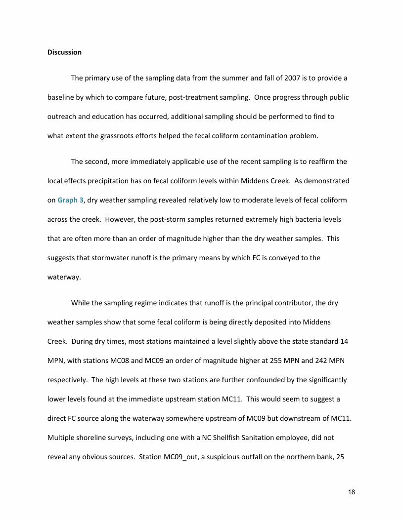
Discussion

The primary use of the sampling data from the summer and fall of 2007 is to provide a

baseline by which to compare future, post-treatment sampling. Once progress through public

outreach and education has occurred, additional sampling should be performed to find to

what extent the grassroots efforts helped the fecal coliform contamination problem.

The second, more immediately applicable use of the recent sampling is to reaffirm the

local effects precipitation has on fecal coliform levels within Middens Creek. As demonstrated

on Graph 3, dry weather sampling revealed relatively low to moderate levels of fecal coliform

across the creek. However, the post-storm samples returned extremely high bacteria levels

that are often more than an order of magnitude higher than the dry weather samples. This

suggests that stormwater runoff is the primary means by which FC is conveyed to the

waterway.

While the sampling regime indicates that runoff is the principal contributor, the dry

weather samples show that some fecal coliform is being directly deposited into Middens

Creek. During dry times, most stations maintained a level slightly above the state standard 14

MPN, with stations MC08 and MC09 an order of magnitude higher at 255 MPN and 242 MPN

respectively. The high levels at these two stations are further confounded by the significantly

lower levels found at the immediate upstream station MC11. This would seem to suggest a

direct FC source along the waterway somewhere upstream of MC09 but downstream of MC11.

Multiple shoreline surveys, including one with a NC Shellfish Sanitation employee, did not

reveal any obvious sources. Station MC09_out, a suspicious outfall on the northern bank, 25

18

feet upstream of MC09, was established during this investigation, however no fecal coliform

was found in the water sample. A review of sampling records from the adjacent Smyrna

Elementary School septic field similarly did not indicate any sources. Alternatively, the source

could be wildlife that is concentrated in this small, wooded section of the creek. Increased

development would decrease habitat for wild animals, and the small section of natural area

around stations MC08 and MC09 could provide the only refuge. This concentration of animals

provides a convenient explanation for the dry weather fecal coliform in the absence of other

identifiable sources.

While future studies could target this stretch of the waterway to find potential fecal

coliform sources, the extreme variation in levels is likely due to water volume at the sampling

sites. MC08 and MC09 are found in shallow water, while MC11 is located in relatively deep

water. The Middens Creek sampling regime showed an increase in FC levels as stations moved

upstream. These results are typical in studies of bacteria within tidal waterways, and it has

been hypothesized that this is due to changes in turbidity, salinity, and temperature (Mallin et

al 2000). These predictors, however, could be proxy measures for water depth. Some studies

suggest that the sediment at the bottom could act as a source of FC, protecting the bacteria

until resuspended (Mallin et al 2000). This resuspension would occur more readily in

shallower water, potentially explaining the inverse relationship between water depth and fecal

coliform levels. However, an investigation testing this hypothesis failed to support the idea.

At station MC09, after a normal water sample was taken, a second collection, MC09_sed, was

performed after significantly stirring up the bottom sediment. Although the turbidity

increased, the fecal coliform levels remained the same as shown in Graph 4. While this is a

19

one sample study, and limited inferences can be made, it suggests a different explanation. It is

possible that water volume alone explains the variation. If there is a natural, constant FC

source along this stretch of creek, the concentration would be much higher in the shallow, low

volume water of stations MC08 and MC09 then in the deeper, high volume MC11 water.

Future studies in the waterway could examine this possibility.

The shoreline survey data provides an accurate assessment of the current state of the

creek including areas that are exacerbating the runoff problem. The engineered shorelines

such as riprap and bulkhead no longer serve their natural function, including nursery area and

water filtration. Much of the shoreline is also lined by suboptimal vegetated buffer.

Vegetated buffers are useful in mitigating stormwater impacts because it provides some

filtration and sink functions. As the stormwater moves laterally across the ground, it gains

speed when traveling across impervious surfaces or manicured lawn. If allowed to speed

toward the waterway, the runoff will deliver any pollutants that are picked up, including fecal

coliform, directly to the water. Vegetated buffers can physically filter this water through both

its above and below ground structures, and also slows the lateral movement to allow time for

pollutants to precipitate out (Desbonnet et al 1995) or for bacteria to die off. Finally, the

vegetation takes up part of the water and transpires it into the ambient air, lessening the

volume of stormwater runoff. Theoretically, the wider the vegetated buffer, the better the

mitigation potential. In the low-lying Middens Creek area, 20’ of vegetated buffer was

selected as an appropriate optimal recommendation due to the balance between effectiveness

and feasibility.

20

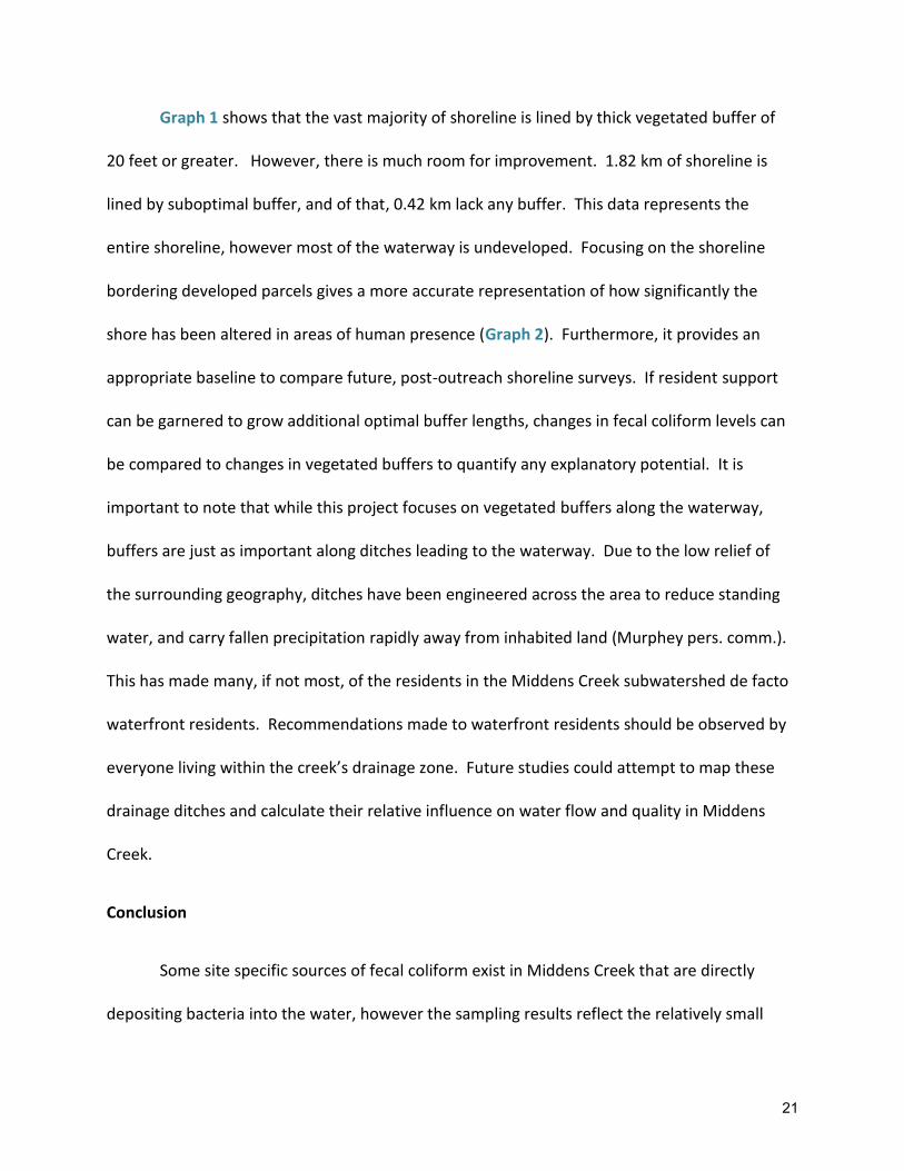
Graph 1 shows that the vast majority of shoreline is lined by thick vegetated buffer of

20 feet or greater. However, there is much room for improvement. 1.82 km of shoreline is

lined by suboptimal buffer, and of that, 0.42 km lack any buffer. This data represents the

entire shoreline, however most of the waterway is undeveloped. Focusing on the shoreline

bordering developed parcels gives a more accurate representation of how significantly the

shore has been altered in areas of human presence (Graph 2). Furthermore, it provides an

appropriate baseline to compare future, post-outreach shoreline surveys. If resident support

can be garnered to grow additional optimal buffer lengths, changes in fecal coliform levels can

be compared to changes in vegetated buffers to quantify any explanatory potential. It is

important to note that while this project focuses on vegetated buffers along the waterway,

buffers are just as important along ditches leading to the waterway. Due to the low relief of

the surrounding geography, ditches have been engineered across the area to reduce standing

water, and carry fallen precipitation rapidly away from inhabited land (Murphey pers. comm.).

This has made many, if not most, of the residents in the Middens Creek subwatershed de facto

waterfront residents. Recommendations made to waterfront residents should be observed by

everyone living within the creek’s drainage zone. Future studies could attempt to map these

drainage ditches and calculate their relative influence on water flow and quality in Middens

Creek.

Conclusion

Some site specific sources of fecal coliform exist in Middens Creek that are directly

depositing bacteria into the water, however the sampling results reflect the relatively small

21

proportion. The largest influence on bacteria loading within the waterway is stormwater

runoff as highlighted by comparing the dry and wet weather sampling. The large jump in fecal

coliform sampling results immediately following a storm suggests that mitigation efforts and

studies should focus on controlling runoff in the subwatershed. The sampling results also

provide a dataset that future sampling efforts can be compared to. After public outreach

efforts have achieved a measurable change in landuse and behavior, future sampling will

provide quantifiable descriptions of the impacts of these changes. This information can then

be used to target the most efficient methods within Middens Creek, and can also be applied to

other coastal waterways experiencing similar declines in water quality.

The shoreline survey reporting lengths of the three buffer categories helps to target

areas where public outreach efforts can focus grassroots change. Identifying the locations of

suboptimal buffer allows the associated parcel of land to be identified and the owner to be

contacted to try and gather support. This method will likely prove more efficient than mass

communication such as bulk mailings. The data reflecting shoreline buffers along developed

parcels further focuses the outreach efforts as it excludes undeveloped property that is

beyond the scope of this project. If significant lengths of suboptimally buffered shoreline

could become more highly vegetated, future sampling and shoreline surveys could measure

their correlation and provide valuable information for stormwater mitigation in other

subwatersheds.

22

Phase III: Historical/Spatial Data Analysis

Introduction

Short-term sampling offers excellent resolution of fecal coliform variations associated

with precipitation fluctuations, but it does not provide context of how landuse changes over

time affect water quality. Examining the impact of human development necessitates the use

of historical water quality, precipitation, and development data. By overlaying these different

data types upon each other, trends become evident both spatially and statistically. The trends

make it apparent that the human presence in the watershed has degraded water quality,

although specific causes are hard to identify. However, in conjunction with the 2007 sampling

that identified stormwater as a significant source of FC, the historical trends give some insight

in how to best reverse the degradation.

Methods

Data Origins:

Obtaining historical fecal coliform data is central to the analysis, and was provided by

NC Shellfish Sanitation. Annual geomean data was supplied for sampling station 65 on

Middens Creek, which is quite close to this study’s station MC01 as shown on Figure 4.

Although records of FC levels date back to the early 1980s, 1998 was the first year the section

used current testing, analysis, and summarization methods. For this reason, only the 1998-

2007 fecal coliform data for the waterway was examined, and only 1998-2006 data was

incorporated into the statistical analysis due to temporal limitations of the county parcel data.

23

Annual total precipitation data was obtained from the State Climate Office at North

Carolina State University. The closest precipitation monitoring station with complete records

spanning the time frame of this study was located in Morehead City, NC, and is identified as

“Morehead City 2 NWN (315830)”. This station, located approximately 10 miles from Middens

Creek, was deemed sufficiently close to represent precipitation levels in the area.

Determining the relevant area surrounding Middens Creek required identification of

the subwatershed that drains into the waterway. Using an elevation data layer obtained from

a LIDAR derived dataset, distributed by the North Carolina Department of Transportation, the

subwatershed was drawn in a Geographic Information System (GIS) by tracing along the

elevation peaks surrounding the creek. The subwatershed encompasses all the adjacent land

that drain into Middens Creek as opposed to other, nearby waterways (Figure 7).

Development information was collected from the Carteret County Tax Office. The

spatial data displayed parcel boundaries and included the year the property was developed

and the total square footage of the houses built between 1700 and 2006. Obtaining spatially

represented data was imperative to ensure that only the relevant properties were included in

the analysis.

To investigate the level of developed shoreline, two shapefiles were created in a GIS

displaying segments along the waterway bordering developed versus undeveloped parcels of

land. These shapefiles were created by tracing along a shoreline outline overlaid by developed

versus undeveloped parcel data and adding these tracings to either the developed or

24

undeveloped shoreline shapefiles respectively. Figure 8 shows the stretches of shoreline

bordering developed versus undeveloped property.

Data Analysis:

The historical fecal coliform data from Shellfish Sanitation shows increasing levels of

the bacteria from 1998 to 2006 as shown in Graph 5. In 2007, levels dropped to near 2002

levels, however this is likely due to the widespread drought engulfing the Southeast US in

2007. Graph 5 also displays the annual precipitation total for the area and reflects the 2007

drought. Less precipitation would dampen stormwater’s impact on bacteria levels within the

creek. Nevertheless, this historical data clearly demonstrates the fecal coliform problem and

the appropriateness of the recent expansion of permanent shellfish closures within the

waterway.

The Middens Creek subwatershed determined from the LIDAR elevation data is shown

in Figure 7. Within a GIS, the spatial county tax data showing the property boundary for

parcels in the area was clipped leaving only those parcels, and portions of parcels, within the

determined subwatershed as shown in Figure 9. This allowed for an analysis of landuse based

only on those properties that contribute stormwater to Middens Creek.

Correlation Study:

With both historical fecal coliform data and development records of applicable areas

surrounding the waterway, a statistical analysis was performed to investigate the correlation

between human presence and bacteria levels within Middens Creek. The first and most

25

obvious variable to investigate was impervious cover. Attempts were made to locate aerial

photographs from which percent impervious surface calculations could be performed.

However, only 2 aerial photographs could be obtained; far fewer than the number needed to

perform a useful regression. In lieu of this data, two different predictor variables were used as

a proxy measure for the extent of development within the creek: number of houses and total

square footage of houses. Each of these variables were determined by parsing out the county

tax data by year, and calculating the total number of houses and square footage of houses for

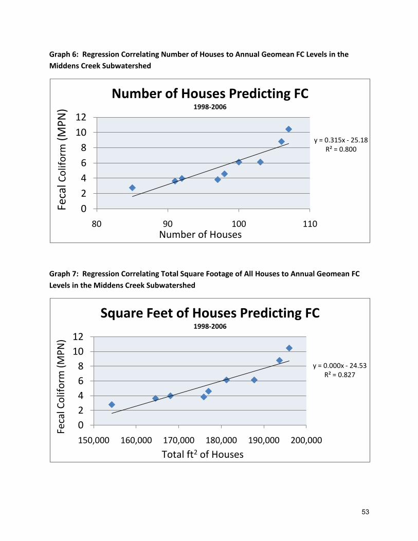
each year between 1998 and 2006. A regression analysis was employed using these predictor

variables to describe historical fecal coliform variation during the target years. An R2 value of

0.800 was reached using total number of houses as the predictor variable, while total square

footage of houses gave an R2 value of 0.827. These results can be seen graphically in Graphs 6

and 7 respectively.

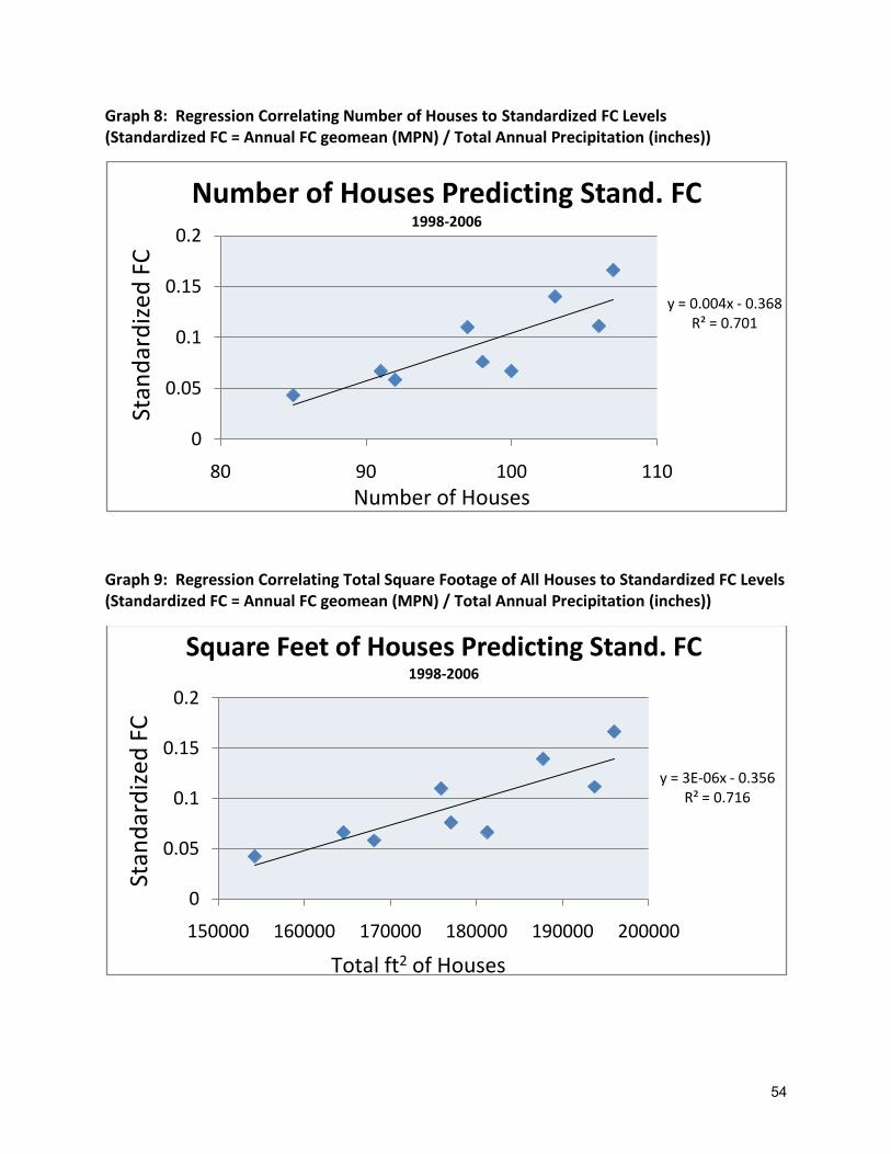
A second set of regressions was performed using a standardized fecal coliform value

calculated by dividing the annual geomean of fecal coliform by the total annual rainfall in the

area. Using total number of houses to describe standardized FC returned a R2 of 0.701 while

the predictor total square footage of houses returned an R2 value of 0.716. Both of these

results can be seen in Graphs 8 and 9 respectively.

Development Progress and Potential:

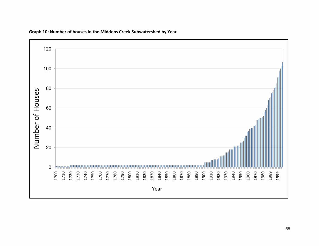
Graph 10 displays the historical rate of house construction within the subwatershed

from 1700 to 2006. To examine the potential for future development, the parcels within the

subwatershed that have been developed were identified (Figure 10) and separated from the

26

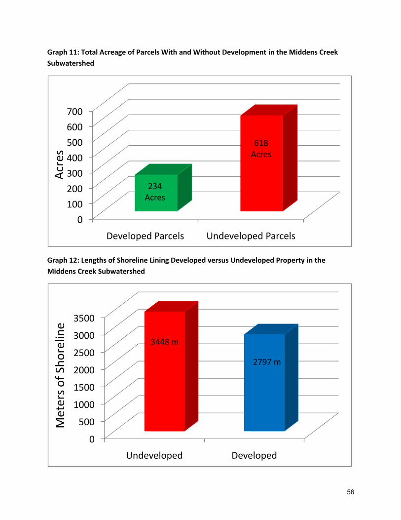
undeveloped parcels in the GIS. The total area of both developed and undeveloped parcels

was calculated resulting in 234 acres of developed parcels and 618 acres of undeveloped

parcels as displayed in Graph 11. Using this data, a rough estimate of the potential for future

housing construction was reached. With a current level of 107 houses within the

subwatershed, and 234 acres of developed lots, an average lot size of 2.2 acres was reached

(234 acres of developed parcels / 107 Houses). Dividing this average lot size into the

undeveloped parcel area of 618 acres results in 281 additional houses (618 acres of

undeveloped parcels / 2.2 acres per house).

Waterfront development potential was also examined by exploring lengths of shoreline

along developed versus undeveloped properties. Within a GIS, the lengths of each of the

shapefiles were calculated and are displayed in Graph 12. The lengths are spatially displayed

in Figure 8.

Discussion

Correlation Study:

All four regressions showed a high degree of correlation with R2 values in the 0.70 and

0.80 range. Specifically, the best correlations were found when using the non-standardized

fecal coliform levels. The R2 value when total square footage of houses within the

subwatershed is used to predict non-standardized FC levels is 0.827. Explaining 83% of the

variation in FC levels strictly through this predictor variable is quite compelling, particularly in

environmental sciences where this level of correlation is uncommon. However, square

footage of houses is only a proxy measure for some other explanatory variable; potentially

27

number of people, septic tank usage, or levels of impervious cover. However, larger houses

don’t necessarily reflect more people due to current trends of increased home size (NAIB

2007). It also isn’t an exact measurement of impervious surface since it doesn’t take into

account driveways and sidewalks, and can overestimate the house’s footprint by a factor of

two if it is a two-story home.

The predictor variable number of houses is similarly ambiguous, since increased

housing doesn’t directly increase FC levels. The correlation is, however, high as well with an R2

value of 0.800. This provides compelling evidence that something associated with the

increased number of houses is causing the increase in fecal coliform. Associated variables

include septic tanks, impervious cover, pets, and engineered stormwater conveyance systems.

While the exact explanation remains elusive with this correlation study, it is quite evident that

increased human presence in the watershed is resulting in increased fecal coliform levels.

The second set of regressions used the same two predictor variables, but substituted

the standardized FC as the response variable. The standardized FC score was calculated by

dividing the annual geomean of fecal coliform by the total annual precipitation. This provided

a fecal coliform value that was independent of precipitation. Using this value is particularly

useful in this study, where assumptions were made linking low 2007 FC levels and drought

conditions. The R2 values dropped slightly but remained quite high with 0.701 and 0.716 for

the variables number of houses and total square footage respectively. These lower strength

correlations are potentially more accurate since it takes precipitation variability out. Although

the R2 is lower using the standardized FC as a predictor, it is still a significant correlation. This

28

significant correlation suggests that human presence within the watershed is affecting fecal

coliform levels independently of rainfall levels.

Development Progress and Potential:

Graph 10, showing the historical development trend within the subwatershed,

demonstrates the exponential growth that began at the beginning of the 20th century and

continues through today. Based on this trend, it is reasonable to assume that development

will continue at this pace into the foreseeable future. Development is increasing at an

increasing rate which will likely exacerbate any anthropogenic problems in Middens Creek.

The future development potential determined through the average lot size and undeveloped

acreage calculations shows just how much more development can occur in the subwatershed.

The conservative value of 2.2 acres per house gives a rough estimate of room for an additional

281 houses. While exact predictions are difficult to make with this type of extrapolation, the

message is quite clear. The area around Middens Creek has just begun to be developed. Any

negative impacts form the human presence will likely continue if status quo management

practices remain.

Along the waterfront, the majority of shoreline borders undeveloped parcels of land

(Graph 12). This observation reiterates the finding that development within the watershed is

just beginning, and there exists plenty of room for over 100% more shoreline development.

Any water quality degradation linked directly to human presence in the subwatershed will

likely intensify as development continues.

29

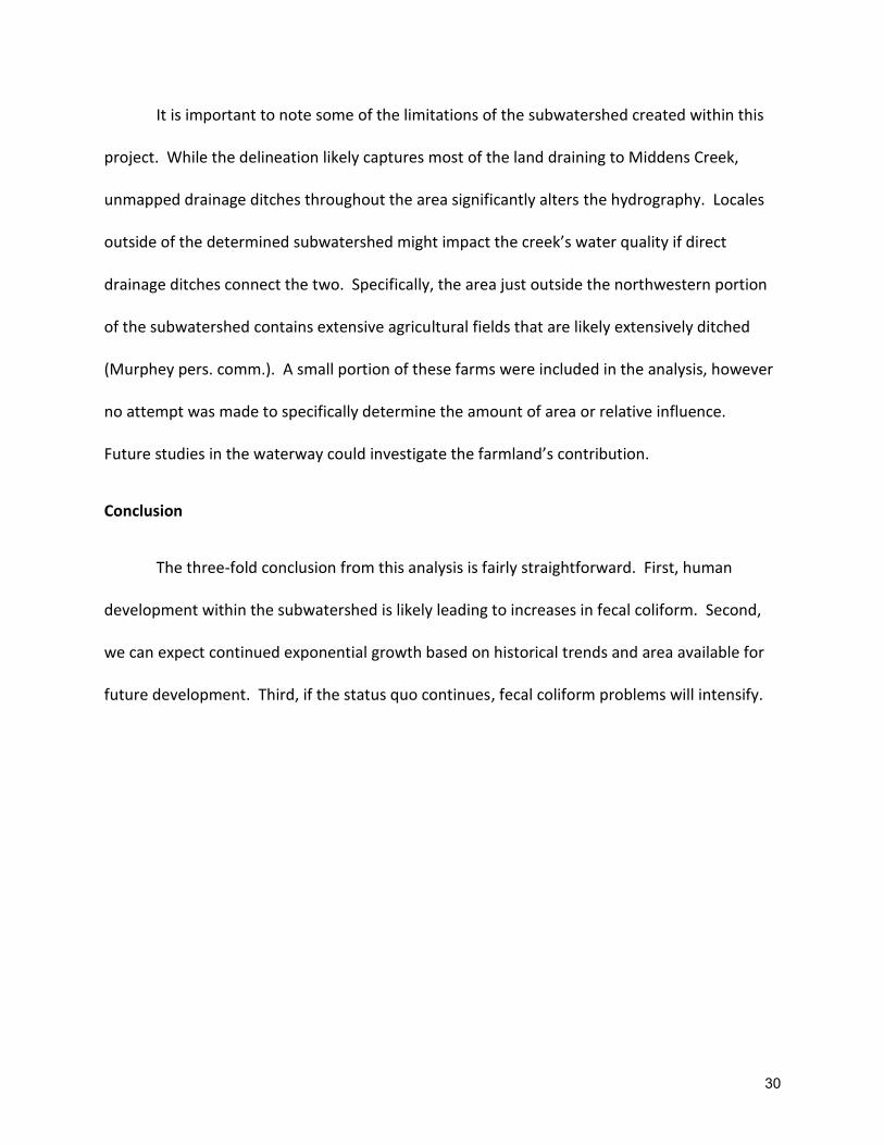
It is important to note some of the limitations of the subwatershed created within this

project. While the delineation likely captures most of the land draining to Middens Creek,

unmapped drainage ditches throughout the area significantly alters the hydrography. Locales

outside of the determined subwatershed might impact the creek’s water quality if direct

drainage ditches connect the two. Specifically, the area just outside the northwestern portion

of the subwatershed contains extensive agricultural fields that are likely extensively ditched

(Murphey pers. comm.). A small portion of these farms were included in the analysis, however

no attempt was made to specifically determine the amount of area or relative influence.

Future studies in the waterway could investigate the farmland’s contribution.

Conclusion

The three-fold conclusion from this analysis is fairly straightforward. First, human

development within the subwatershed is likely leading to increases in fecal coliform. Second,

we can expect continued exponential growth based on historical trends and area available for

future development. Third, if the status quo continues, fecal coliform problems will intensify.

30

Phase IV: Public Outreach and Education

Based on the conclusions reached from the first three phases of the project, public

outreach was the most direct and effective way to affect real change in water quality

degradation within Middens Creek. The fecal coliform characterization sampling confirms that

stormwater is the primary conveyance system for the bacteria, and there is a strong statistical

correlation showing that human presence in the watershed is likely the primary factor. Policy

proposals currently before the state legislature could prove beneficial in mitigating stormwater

from future development, but it does not address problems caused by existing development.

Short of additional legislation targeting this inadequacy, the only means to stop or reverse the

impacts of established development is through public outreach and education. By educating

the residents of Middens Creek about their contribution to bacteria loading in the waterway, a

concerted grassroots attempt can be made to mitigate nonpoint fecal coliform sources.

During the late winter and early spring of 2008, outreach efforts began to rally support

and volunteers for grassroots change. A presentation was developed outlining this project’s

findings as well as some background information on fecal coliform, shellfish, and stormwater.

The Microsoft Office PowerPoint Presentation portion is attached in Appendix 1. This

information was presented to a number of groups including Carteret County Crossroads, NC

Shellfish Sanitation, and the Department of Health, however the most directly impactful

presentation was to a group of residents that live in the Middens Creek subwatershed. In

February 2008, a group of about 23 residents from 13 households convened at Smyrna

Elementary School to learn about the project. Recognizing that the audience members were a

biased sampling of residents since the presentation was made to those who voluntarily

31

attended an evening environmental outreach meeting, there was a positive response to the

meeting and much support was garnered. Of the 23 residents, 8 expressed immediate interest

in building a raingarden, 5 in installing a cistern, 4 in having their septic tanks inspected and

pumped out, and 3 in developing a vegetated buffer. Information was handed out on other

ways to mitigate stormwater impacts and reduce fecal coliform sources, and references were

offered for further investigation. This initial meeting is potentially the first of several that will

occur after the publication of this project. Additional resident participation will be developed

through word of mouth, additional meetings, and a short DVD that was produced containing a

video of a live presentation of this project. Post-treatment sampling after the conclusion of

the public outreach phase can be compared to the 2007 fecal coliform sampling to quantify

any changes.

32

Project Conclusion:

The purpose of this project is to serve as a foundation for future inquires into water

quality mitigation within Middens Creek. Determining that the primary conveyance for fecal

coliform is stormwater and that human presence in the watershed is likely the root cause,

helps to focus current and future efforts aimed at mitigating water quality impacts in the

waterway. A variety of solutions exist to decrease bacterial loading within Middens Creek, to

prevent additional shellfishing closures, and to reestablish harvestable beds in the closed

portions of the waterway. However, only a small subset of solutions are feasible. The first and

most obvious solution is to pass the current coastal stormwater rule amendments that would

result in increased runoff control. However, with the proposed amendments facing uncertain

approval, other solutions must be evaluated and pursued to ensure that the goals are met. In

lieu of definitively effective regulations to reduce stormwater impacts on shellfishing grounds,

public outreach and education is the only logical course of action. Educating residents within

shellfishing watersheds about the impacts of stormwater and what they can do to slow and

stop their contribution to the problem is the most effective option we have to stop and

reverse the decline in coastal water quality. Testing this course of action is particularly

convenient within the Middens Creek watershed due to the low population density. Outreach

efforts continue to be manageable because of the small scale, and a variety of approaches can

be tested. Likely, the most effective approach will be assisting with the construction of

stormwater control measures to slow or prevent runoff from entering the waterway. These

will include measures such as vegetated buffers, green roofs, rain gardens, rain barrels, and

pervious driveways. The success of this grassroots approach hinges on the assumption that

33

the residents of a waterway will be particularly inclined to embrace these measures. Lessons

learned from the Middens Creek process will prove valuable in assessing this assumption and

will hopefully provide a mitigation methodology for other similarly inflicted waterways.

34

References Cited: American Public Health Association (1995) Standard Methods for the Examination of Water and Wastewater. 19th Edition. American Public Health Association, Washington, DC. USA. Carteret County Tax Records Office. (2007). Geospatial Information Systems ESRI Shapefile. Copeland, Claudia. (January 24, 2002). Clean Water Act: A Summary of the Law. Congressional Research Service Report for Congress. Retrieved November 26, 2007, from the World Wide Web: http://usinfo.state.gov/usa/infousa/laws/majorlaw/cwa.pdf Dadswell, J. V. (1993). Microbiological quality of coastal waters and its health effects. International Journal of Environmental Health Research 3:32-46. Desbonnet, Alan, Virginia Lee, Pamela Pogue, David Reis, James Boyd, Jeffrey Willis, Mark Imperial. (1995). Development of Coastal Vegetated Buffer Programs. Coastal Management, 23, 91-109. Environmental Protection Agency (EPA). (2003). Introduction to the Clean Water Act Module. Retrieved November 26, 2007 from the World Wide Web: http://www.epa.gov/watertrain/cwa/ Environmental Protection Agency (EPA). (2005). Stormwater Phase II Final Rule: An Overview. Retrieved November 26, 2007 from the World Wide Web: http://www.epa.gov/npdes/pubs/fact1-0.pdf Environmental Protection Agency (EPA). (2007a). National Pollutant Discharge Elimination System Overview. Retrieved November 26, 2007 from the World Wide Web: http://cfpub.epa.gov/npdes/ Environmental Protection Agency (EPA). (2007b). Clean Water Act History. Retrieved November 26, 2007 from the World Wide Web: http://www.epa.gov/region5/water/cwa.htm Environmental Protection Agency (EPA). (2007c). Phases of the NPDES Stormwater Program. Retrieved November 26, 2007 from the World Wide Web: http://cfpub.epa.gov/npdes/stormwater/swphases.cfm Federal Wildlife Laws Handbook. (1998). Federal Water Pollution Control Act (Clean Water Act). Center For Wildlife Law. University of New Mexico School of Law, Institute of Public Law. Retrieved November 26, 2007, from the World Wide Web: http://ipl.unm.edu/cwl/fedbook/fwpca.html Fowler, Patricia. Assistant Section Chief, North Carolina Shellfish Sanitation. Personal Communication. June 2007.

35

Giese, G L., H. B. Wilder, G. G. Parker. (1985) Hydrology of Major Estuaries and Sounds of North Carolina. Raleigh, NC: USGS. , USGS Water-Supply Paper 2221. Klimeck, Alan. (2005). North Carolina Division of Water Quality. Directors Memo: Issuance of General Permit for the National Pollutant Discharge Elimination System (NPDES) Phase 2 Stormwater Permitting Program. Retrieved November 26, 2007 from the World Wide Web: http://h2o.enr.state.nc.us/su/documents/Directors_memo.pdf Lin, Jing, Lian Xie, Leonard J. Pietrafesa, Joseph S. Ramus and Hans W. Paerl . (2007) Water quality gradients across Albemarle-Pamlico estuarine system: seasonal variations and model applications. Journal of Coastal Research, 23.1, 213- 230. Mallin, Michael A., Kathleen E. Williams, E. Cartier Esham, R. Patrick Lowe. (2000). Effect of Human Development on Bacteriological Water Quality in Coastal Watersheds. Ecological Applications, 10, 1047-1056. Mallin, Michael A., Scott H. Ensign, Matthew R. McIver, G. Christopher Shank and Patricia K. Fowler. (2001). Demographic, landscape, and meteorological factors controlling the microbial pollution of coastal waters. Hydrobiologia, 460, 185-193. Murphey, Steve. Environmental Supervisor (Inspection Program), North Carolina Shellfish Sanitation. Personal Communication. 3 March 2008. National Association of Home Builders (NAIB). July 25 2007 “Single-Family Square Footage by Location”. Retrieved March 10 2008 from the World Wide Web: http://www.nahb.org/fileUpload_details.aspx?contentID=80051 North Carolina Division of Water Quality. (January 2007). North Carolina’s Basinwide Approach to Water Quality Management. NCDWQ Draft Executive Summary. Retrieved November 26, 2007, from the World Wide Web: http://h2o.enr.state.nc.us/basinwide/documents/ExecutiveSummary_024.pdf North Carolina Division of Water Quality (DWQ). (2007a). Stormwater Unit:: NPDES Phase I Stormwater Program. Retrieved November 26, 2007 from the World Wide Web: http://h2o.enr.state.nc.us/su/NPDES_Phase_I_Stormwater_Program.htm North Carolina Division of Water Quality (DWQ). (2007b). Phase II Stormwater. Retrieved November 26, 2007 from the World Wide Web: http://www.ncphase2sw.org/whatphase2.htm North Carolina Division of Water Quality (DWQ). (2007c). Stormwater Unit:: NPDES Phase II Stormwater Program. Retrieved November 26, 2007 from the World Wide Web: http://h2o.enr.state.nc.us/su/NPDES_Phase_II_Stormwater_Program.htm

36

North Carolina Division of Water Quality (DWQ). (2007d). Stormwater Unit:: State Stormwater Management Program. Retrieved November 26, 2007 from the World Wide Web: http://h2o.enr.state.nc.us/su/state_sw.htm North Carolina Division of Water Quality (DWQ). (2007e). Economic Assessment and Justification for Proposed Amendments to 15A NCAC 2H .1005, the Coastal Stormwater Rules. Retrieved November 26, 2007 from the World Wide Web: http://h2o.enr.state.nc.us/su/documents/CoastalRuleAmendments-EconomicAssessment.doc North Carolina Department of Health (DEH). (2006). Report of Sanitary Survey Area E-8 and E-9: March 2001 through March 2006. Prepared by the Shellfish Sanitation and Recreational Water Quality Section of the NC Division of Environmental Health, April 2006. Orbach, Michael. (2007). Marine Policy Lecture. Duke University Marine Lab. Fall 2007. Paerl, Hans W., Jerad D. Bales, Larry W. Ausley, Christopher P. Buzzelli, Larry B. Crowder, Lisa A. Eby, John M. Fear, Malia Go, Benjamin L. Peierls, Tammi L. Richardson, Joseph S. Ramus . 2001 May 8. Ecosystem impacts of three sequential hurricanes (Dennis, Floyd, and Irene) on the United States' largest lagoonal estuary, Pamlico Sound, NC. Ecology, 98(10): 5655–5660. Rawlins, Wade. North Carolina Coastal Federation. (October 10, 2007). Tougher Rules Likely on Stormwater Runoff. North Carolina Coastal Federation Press Release. Retrieved November 26, 2007, from the World Wide Web: http://www.nccoast.org/news/nostormwater Wynn, Lori. “Coastal Rules Return to EMC for Changes.” Carteret County News-Times February 22, 2007, Vol 97-No 23: 1A.

37

Figures:

Figure 1: Reference Map for the Location of Middens Creek

p. 39

Figure 2: Map of Shellfish Closure Line in Middens Creek Before and After the 2007

Shellfish Sanitation Recommendations.

p. 40

Figure 3: 20 Coastal North Carolina Counties with the 3 NPDES Phase II Stormwater

Program Counties in Yellow

p. 41

Figure 4: Middens Creek Project and State Sampling Station Locations

p. 42

Figure 5: Vegetated Buffer Width along the Shoreline in Middens Creek

p. 43

Figure 6: Vegetated Buffer Width along the Developed Shoreline Only

p. 44

Figure 7: Subwatershed of Middens Creek

p. 45

Figure 8: Shoreline Bordering Developed and Undeveloped Parcels of Land

p. 46

Figure 9: Parcels and Portions of Parcels within the Middens Creek Subwatershed

p. 47

Figure 10: Undeveloped Parcels within Middens Creek Subwatershed

p. 48

38

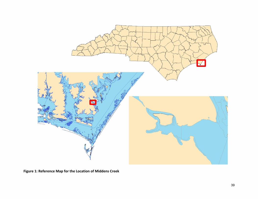
Figure 1: Reference Map for the Location of Middens Creek

39

Figure 2: Map of Shellfish Closure Line in Middens Creek Before and After the 2007 Shellfish Sanitation Recommendations.

40

Figure 3: 20 Coastal North Carolina Counties with the 3 NPDES Phase II Stormwater Program Counties in Yellow

41

Figure 4: Middens Creek Project and State Sampling Station Locations

42

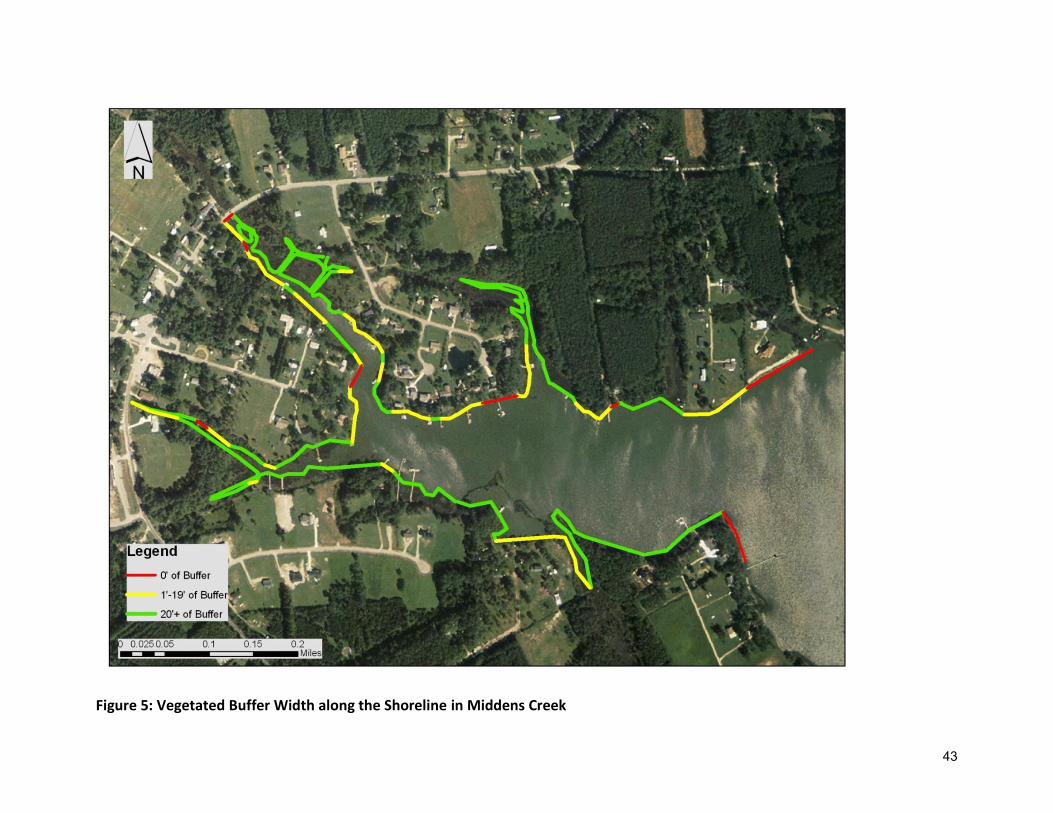
Figure 5: Vegetated Buffer Width along the Shoreline in Middens Creek

43

Figure 6: Vegetated Buffer Width along the Developed Shoreline Only

44

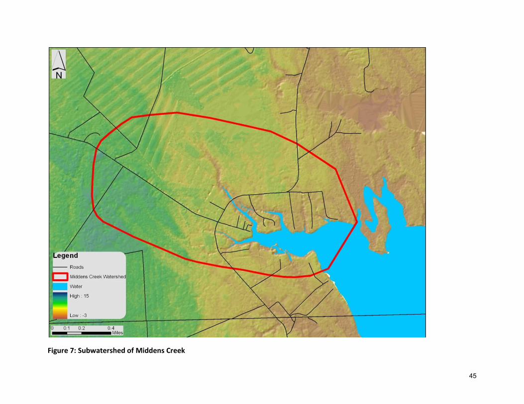
Figure 7: Subwatershed of Middens Creek

45

Figure 8: Shoreline Bordering Developed and Undeveloped Parcels of Land

46

Figure 9: Parcels and Portions of Parcels within the Middens Creek Subwatershed

47

Figure 10: Undeveloped Parcels within Middens Creek Subwatershed

48

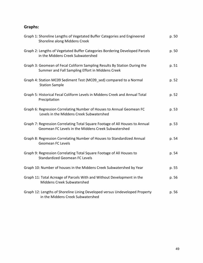
Graphs:

Graph 1: Shoreline Lengths of Vegetated Buffer Categories and Engineered Shoreline along Middens Creek

p. 50

Graph 2: Lengths of Vegetated Buffer Categories Bordering Developed Parcels in the Middens Creek Subwatershed

p. 50

Graph 3: Geomean of Fecal Coliform Sampling Results By Station During the Summer and Fall Sampling Effort in Middens Creek

p. 51

Graph 4: Station MC09 Sediment Test (MC09_sed) compared to a Normal Station Sample

p. 52

Graph 5: Historical Fecal Coliform Levels in Middens Creek and Annual Total Precipitation

p. 52

Graph 6: Regression Correlating Number of Houses to Annual Geomean FC Levels in the Middens Creek Subwatershed

p. 53

Graph 7: Regression Correlating Total Square Footage of All Houses to Annual Geomean FC Levels in the Middens Creek Subwatershed

p. 53

Graph 8: Regression Correlating Number of Houses to Standardized Annual Geomean FC Levels

p. 54

Graph 9: Regression Correlating Total Square Footage of All Houses to Standardized Geomean FC Levels

p. 54

Graph 10: Number of houses in the Middens Creek Subwatershed by Year

p. 55

Graph 11: Total Acreage of Parcels With and Without Development in the Middens Creek Subwatershed

p. 56

Graph 12: Lengths of Shoreline Lining Developed versus Undeveloped Property in the Middens Creek Subwatershed

p. 56

49

Graph 1: Shoreline Lengths of Vegetated Buffer Categories and Engineered Shoreline along

Middens Creek

Graph 2: Lengths of Vegetated Buffer Categories Bordering Developed Parcels in the Middens

Creek Subwatershed

0

500

1000

1500

2000

2500

3000

3500

4000

0' Buffer 1'-19' Buffer 20'+ Buffer Bulkhead/Riprap

422 m

1400 m

3602 m

498 mMet

ers

of

Sho

relin

e

0

200

400

600

800

1000

1200

0' Buffer 1'-19' Buffer 20'+ Buffer

403 m

1129 m 1100 m

Met

ers

of

Sho

relin

e

50

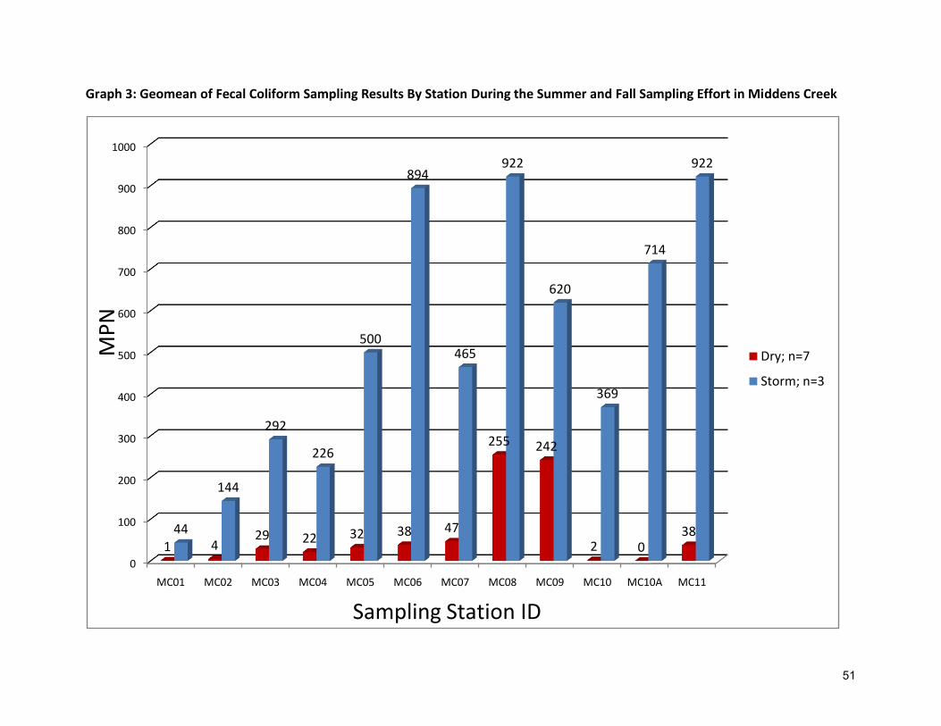
Graph 3: Geomean of Fecal Coliform Sampling Results By Station During the Summer and Fall Sampling Effort in Middens Creek

0

100

200

300

400

500

600

700

800

900

1000

MC01 MC02 MC03 MC04 MC05 MC06 MC07 MC08 MC09 MC10 MC10A MC11

1 429 22 32 38 47

255 242

2 03844

144

292

226

500

894

465

922

620

369

714

922

Dry; n=7

Storm; n=3

MP

N

Sampling Station ID

51

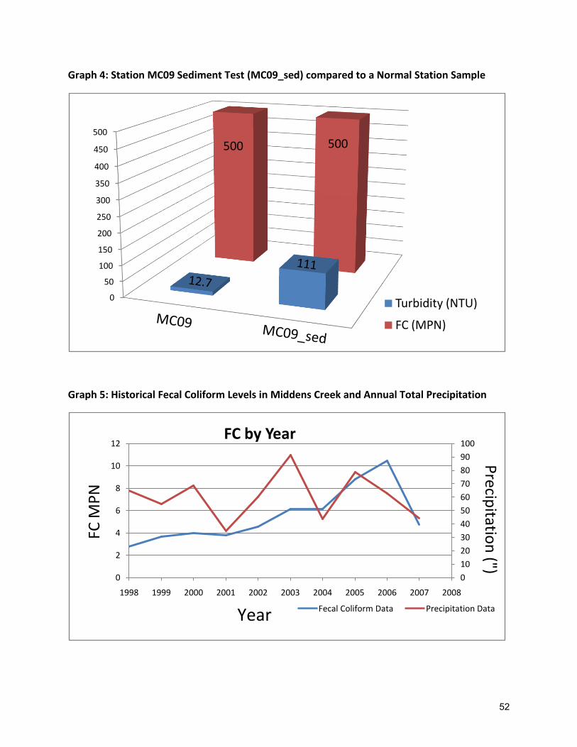
Graph 4: Station MC09 Sediment Test (MC09_sed) compared to a Normal Station Sample

Graph 5: Historical Fecal Coliform Levels in Middens Creek and Annual Total Precipitation

0

50

100

150

200

250

300

350

400

450

500

500 500

Turbidity (NTU)

FC (MPN)

0

10

20

30

40

50

60

70

80

90

100

0

2

4

6

8

10

12

1998 1999 2000 2001 2002 2003 2004 2005 2006 2007 2008

FC by Year

Fecal Coliform Data Precipitation Data

FC M

PN

Year

Precip

itation

(")

52

Graph 6: Regression Correlating Number of Houses to Annual Geomean FC Levels in the

Middens Creek Subwatershed

Graph 7: Regression Correlating Total Square Footage of All Houses to Annual Geomean FC

Levels in the Middens Creek Subwatershed

y = 0.315x - 25.18R² = 0.800

0

2

4

6

8

10

12

80 90 100 110

Number of Houses Predicting FC1998-2006

Feca

l Co

lifo

rm(M

PN

)

Number of Houses

y = 0.000x - 24.53R² = 0.827

0

2

4

6

8

10

12

150,000 160,000 170,000 180,000 190,000 200,000

Square Feet of Houses Predicting FC1998-2006

Feca

l Co

lifo

rm (

MP

N)

Total ft2 of Houses

53

Graph 8: Regression Correlating Number of Houses to Standardized FC Levels (Standardized FC = Annual FC geomean (MPN) / Total Annual Precipitation (inches))

Graph 9: Regression Correlating Total Square Footage of All Houses to Standardized FC Levels (Standardized FC = Annual FC geomean (MPN) / Total Annual Precipitation (inches))

y = 0.004x - 0.368R² = 0.701

0

0.05

0.1

0.15

0.2

80 90 100 110

Number of Houses Predicting Stand. FC1998-2006

Number of Houses

Stan

dar

diz

ed F

C

y = 3E-06x - 0.356R² = 0.716

0

0.05

0.1

0.15

0.2

150000 160000 170000 180000 190000 200000

Square Feet of Houses Predicting Stand. FC1998-2006

Stan

dar

diz

ed F

C

Total ft2 of Houses

54

Graph 10: Number of houses in the Middens Creek Subwatershed by Year

0

20

40

60

80

100

1201

70

0

17

10

17

20

17

30

17

40

17

50

17

60

17

70

17

80

17

90

18

00

18

10

18

20

18

30

18

40

18

50

18

60

18

70

18

80

18

90

19

00

19

10

19

20

19

30

19

40

19

50

19

60

19

70

19

80

19

89

19

99

Nu

mb

er o

f H

ou

ses

Year

55

Graph 11: Total Acreage of Parcels With and Without Development in the Middens Creek

Subwatershed

Graph 12: Lengths of Shoreline Lining Developed versus Undeveloped Property in the

Middens Creek Subwatershed

0

100

200

300

400

500

600

700

Developed Parcels Undeveloped Parcels

234Acres

618Acres

Acr

es

0

500

1000

1500

2000

2500

3000

3500

Undeveloped Developed

3448 m

2797 m

Met

ers

of

Sho

relin

e

56

Tables:

Table 1: Fecal Coliform Result Summary from Summer and Fall 2007 Middens Creek Sampling

p. 58

Table 2: Fecal Coliform Geomean by Sample Type in Middens Creek

p. 59

Table 3: Station Locations in Middens Creek

p. 59

Table 4: Raw Sampling Results from Summer and Fall 2007 Middens Creek Sampling

p. 60

Table 5: Sampling Notes from Summer and Fall 2007 Middens Creek Sampling

p. 64

57

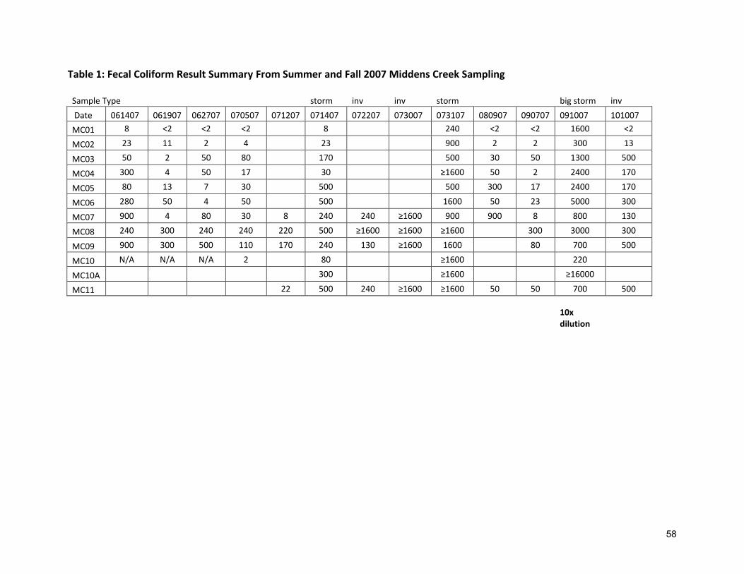
Table 1: Fecal Coliform Result Summary From Summer and Fall 2007 Middens Creek Sampling

Sample Type

storm inv inv storm

big storm inv

Date 061407 061907 062707 070507 071207 071407 072207 073007 073107 080907 090707 091007 101007

MC01 8 <2 <2 <2

8

240 <2 <2 1600 <2

MC02 23 11 2 4

23

900 2 2 300 13

MC03 50 2 50 80

170

500 30 50 1300 500

MC04 300 4 50 17

30

≥1600 50 2 2400 170

MC05 80 13 7 30

500

500 300 17 2400 170

MC06 280 50 4 50

500

1600 50 23 5000 300

MC07 900 4 80 30 8 240 240 ≥1600 900 900 8 800 130

MC08 240 300 240 240 220 500 ≥1600 ≥1600 ≥1600

300 3000 300

MC09 900 300 500 110 170 240 130 ≥1600 1600

80 700 500

MC10 N/A N/A N/A 2

80

≥1600

220

MC10A 300

≥1600

≥16000

MC11

22 500 240 ≥1600 ≥1600 50 50 700 500

10x dilution

58

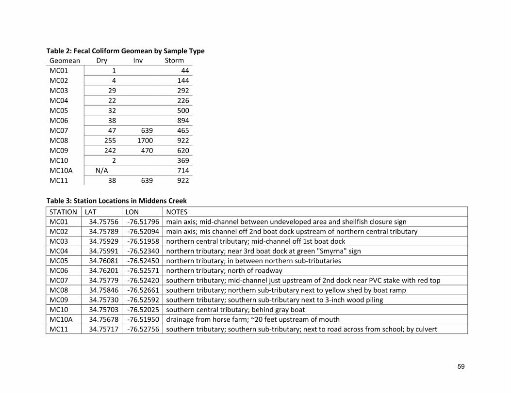
Table 2: Fecal Coliform Geomean by Sample Type Geomean Dry Inv Storm

MC01 1 44

MC02 4 144

MC03 29 292

MC04 22 226

MC05 32 500

MC06 38 894

MC07 47 639 465

MC08 255 1700 922

MC09 242 470 620

MC10 2 369

MC10A N/A 714

MC11 38 639 922

Table 3: Station Locations in Middens Creek

STATION LAT LON NOTES

MC01 34.75756 -76.51796 main axis; mid-channel between undeveloped area and shellfish closure sign

MC02 34.75789 -76.52094 main axis; mis channel off 2nd boat dock upstream of northern central tributary

MC03 34.75929 -76.51958 northern central tributary; mid-channel off 1st boat dock

MC04 34.75991 -76.52340 northern tributary; near 3rd boat dock at green "Smyrna" sign

MC05 34.76081 -76.52450 northern tributary; in between northern sub-tributaries

MC06 34.76201 -76.52571 northern tributary; north of roadway

MC07 34.75779 -76.52420 southern tributary; mid-channel just upstream of 2nd dock near PVC stake with red top

MC08 34.75846 -76.52661 southern tributary; northern sub-tributary next to yellow shed by boat ramp

MC09 34.75730 -76.52592 southern tributary; southern sub-tributary next to 3-inch wood piling

MC10 34.75703 -76.52025 southern central tributary; behind gray boat

MC10A 34.75678 -76.51950 drainage from horse farm; ~20 feet upstream of mouth

MC11 34.75717 -76.52756 southern tributary; southern sub-tributary; next to road across from school; by culvert

59

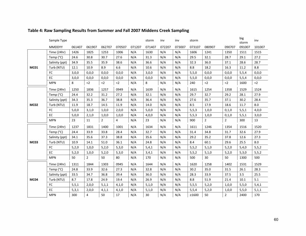
Table 4: Raw Sampling Results from Summer and Fall 2007 Middens Creek Sampling

Sample Type

storm inv inv storm

big storm

inv

MMDDYY 061407 061907 062707 070507 071207 071407 072207 073007 073107 080907 090707 091007 101007

MC01

Time (24hr) 1426 1825 1253 1006 N/A 1630 N/A N/A 1606 1241 1350 1511 1515

Temp (°C) 24.6 30.8 30.7 27.6 N/A 31.3 N/A N/A 29.5 32.1 28.7 29.1 27.2

Salinity (ppt) 34.9 35.5 35.9 38.6 N/A 36.6 N/A N/A 32.3 36.0 37.1 28.6 28.7

Turb (NTU) 12.1 10.9 8.9 6.6 N/A 10.6 N/A N/A 8.8 18.2 16.3 11.2 8.8

FC 3,0,0 0,0,0 0,0,0 0,0,0 N/A 3,0,0 N/A N/A 5,5,0 0,0,0 0,0,0 5,5,4 0,0,0

EC 3,0,0 0,0,0 0,0,0 0,0,0 N/A 0,0,0 N/A N/A 5,5,0 0,0,0 0,0,0 5,5,4 0,0,0

MPN 8 <2 <2 <2 N/A 8 N/A N/A 240 <2 <2 1600 <2

MC02

Time (24hr) 1250 1836 1257 0949 N/A 1639 N/A N/A 1615 1254 1358 1529 1524

Temp (°C) 24.4 32.2 31.2 27.2 N/A 32.1 N/A N/A 29.7 32.7 29.2 28.1 27.9

Salinity (ppt) 34.3 35.3 36.7 38.8 N/A 36.4 N/A N/A 27.6 35.7 37.1 30.2 28.4

Turb (NTU) 11.9 18.7 14.5 11.9 N/A 14.0 N/A N/A 8.5 17.9 18.6 11.7 8.0

FC 5,0,0 3,1,0 1,0,0 2,0,0 N/A 5,0,0 N/A N/A 5,5,3 1,0,0 0,1,0 5,5,1 4,0,0

EC 5,0,0 2,1,0 1,0,0 1,0,0 N/A 4,0,0 N/A N/A 5,5,3 1,0,0 0,1,0 5,5,1 3,0,0

MPN 23 11 2 4 N/A 23 N/A N/A 900 2 2 300 13

MC03

Time (24hr) 1237 1831 1400 1001 N/A 1634 N/A N/A 1611 1246 1354 1516 1520

Temp (°C) 24.4 33.9 33.8 28.4 N/A 32.7 N/A N/A 31.4 34.8 31.7 32.6 27.9

Salinity (ppt) 34.1 35.6 37.3 38.8 N/A 35.6 N/A N/A 29.2 35.2 37.8 12.6 27.3

Turb (NTU) 10.9 14.1 51.0 36.1 N/A 24.8 N/A N/A 8.4 60.1 29.6 25.5 8.0

FC 5,2,0 1,0,0 5,2,0 5,3,0 N/A 5,4,1 N/A N/A 5,5,2 5,1,0 5,2,0 5,4,0 5,5,2

EC 5,2,0 1,0,0 5,2,0 5,3,0 N/A 3,4,1 N/A N/A 5,5,2 5,1,0 5,2,0 5,3,0 5,5,2

MPN 50 2 50 80 N/A 170 N/A N/A 500 30 50 1300 500

MC04

Time (24hr) 1311 1844 1303 0945 N/A 1644 N/A N/A 1620 1258 1402 1531 1529

Temp (°C) 24.8 33.9 32.6 27.3 N/A 32.8 N/A N/A 30.2 35.0 31.5 26.1 28.3

Salinity (ppt) 33.5 34.7 36.8 39.4 N/A 36.0 N/A N/A 28.3 33.9 37.5 3.5 25.5

Turb (NTU) 8.7 17.8 24.9 19.4 N/A 26.9 N/A N/A 8.8 51.9 21.4 10.1 5.1

FC 5,5,1 2,0,0 5,1,1 4,1,0 N/A 5,1,0 N/A N/A 5,5,5 5,2,0 1,0,0 5,5,0 5,4,1

EC 5,3,1 2,0,0 4,1,1 4,1,0 N/A 5,1,0 N/A N/A 5,5,4 5,2,0 1,0,0 5,5,0 5,1,1

MPN 300 4 50 17 N/A 30 N/A N/A ≥1600 50 2 2400 170

60

MMDDYY 061407 061907 062707 070507 071207 071407 072207 073007 073107 080907 090707 091007 101007

MC05

Time (24hr) 1325 1847 1305 0941 N/A 1647 N/A N/A 1622 1304 1405 1533 1530

Temp (°C) 24.9 33.6 32.2 27.6 N/A 32.5 N/A N/A 30.0 32.3 31.0 25.7 28.0

Salinity (ppt) 33.0 34.5 36.9 39.5 N/A 35.2 N/A N/A 24.2 26.9 37.5 0.6 24.9

Turb (NTU) 7.5 17.9 24.9 20.3 N/A 54.5 N/A N/A 5.4 32.0 23.7 8.6 9.7

FC 5,3,0 4,0,0 2,1,0 5,1,0 N/A 5,5,2 N/A N/A 5,5,2 5,5,1 4,1,0 5,5,0 5,4,1

EC 5,2,0 4,0,0 2,1,0 5,1,0 N/A 5,3,2 N/A N/A 5,5,1 5,4,1 4,1,0 5,5,0 5,4,1

MPN 80 13 7 30 N/A 500 N/A N/A 500 300 17 2400 170

MC06

Time (24hr) 1336 1851 1309 0936 N/A 1650 N/A N/A 1626 1306 1409 1535 1532

Temp (°C) 25.1 32.9 31.8 26.7 N/A 32.0 N/A N/A 29.2 34.6 30.4 24.9 27.9

Salinity (ppt) 32.2 33.8 36.2 39.6 N/A 33.6 N/A N/A 24.7 32.4 37.2 0.5 24.9

Turb (NTU) 4.7 17.9 18.5 14.5 N/A 16.0 N/A N/A 8.0 33.0 21.7 13.3 18.2

FC 5,4,3 5,1,1 2,0,0 5,2,0 N/A 5,5,2 N/A N/A 5,5,4 5,2,0 5,0,0 5,5,2 5,5,1

EC 5,4,3 4,2,1 1,0,0 3,2,0 N/A 2,5,2 N/A N/A 5,5,3 5,2,0 5,0,0 5,5,2 5,4,1

MPN 280 50 4 50 N/A 500 N/A N/A 1600 50 23 5000 300

MC07

Time (24hr) 1356 1904 1319 0923 1540 1658 0930 1426 1634 1320 1416 1545 1539

Temp (°C) 24.7 32.8 34.1 26.8 33.3 31.5 25.7 29.8 29.7 35.0 31.2 27.2 28.5

Salinity (ppt) 33.4 34.9 36.2 39.0 39.1 33.9 35.1 35.4 18.2 33.5 37.4 2.3 27.7

Turb (NTU) 13.5 42.0 33.0 29.7 48.9 31.4 9.4 25.2 10.1 82.9 32.6 9.0 11.4

FC 5,5,3 2,0,0 5,3,0 5,1,0 3,0,0 5,5,0 5,5,0 5,5,5 5,5,3 5,5,3 3,0,0 5,3,0 5,4,0

EC 5,5,3 2,0,0 4,3,0 4,1,0 2,0,1 5,4,0 5,5,0 5,5,5 5,5,1 5,5,3 3,0,0 5,4,0 5,3,0

MPN 900 4 80 30 8 240 240 ≥1600 900 900 8 800 130

MC08

Time (24hr) 1407 1910 1326 0915 1447 1703 0935 1431 1638 no water 1424 1550 1546

Temp (°C) 24.7 31.1 31.1 25.4 30.1 30.4 27.1 27.5 27.2 no water 27.4 25.4 26.5

Salinity (ppt) 32.5 32.9 34.6 38.5 29.9 31.5 35.7 30.7 16.2 no water 36.6 0.3 24.1

Turb (NTU) 24.6 24.2 19.9 15.5 36.3 23.0 11.8 16.6 11.8 no water 24.2 8.9 6.7

FC 5,5,0 5,5,1 5,5,0 5,5,0 5,4,2 5,5,2 5,5,5 5,5,5 5,5,5 no water 5,5,1 5,5,1 5,5,1

EC 5,5,0 5,5,1 5,5,0 5,5,0 5,4,2 5,5,2 5,5,5 5,5,5 5,5,5 no water 5,5,1 5,5,1 5,5,1

MPN 240 300 240 240 220 500 ≥1600 ≥1600 ≥1600 no water 300 3000 300

61

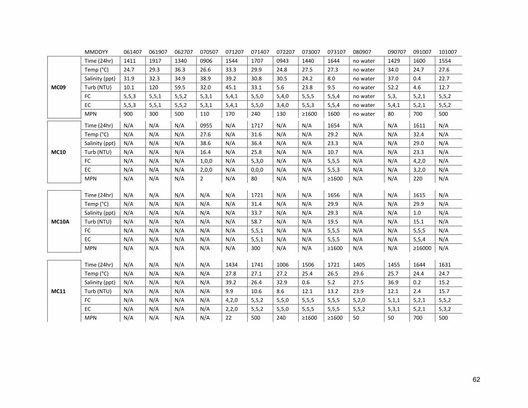
MMDDYY 061407 061907 062707 070507 071207 071407 072207 073007 073107 080907 090707 091007 101007

MC09

Time (24hr) 1411 1917 1340 0906 1544 1707 0943 1440 1644 no water 1429 1600 1554

Temp (°C) 24.7 29.3 36.3 26.6 33.3 29.9 24.8 27.5 27.3 no water 34.0 24.7 27.6

Salinity (ppt) 31.9 32.3 34.9 38.9 39.2 30.8 30.5 24.2 8.0 no water 37.0 0.4 22.7

Turb (NTU) 10.1 120 59.5 32.0 45.1 33.1 5.6 23.8 9.5 no water 52.2 4.6 12.7

FC 5,5,3 5,5,1 5,5,2 5,3,1 5,4,1 5,5,0 5,4,0 5,5,5 5,5,4 no water 5,3, 5,2,1 5,5,2

EC 5,5,3 5,5,1 5,5,2 5,3,1 5,4,1 5,5,0 3,4,0 5,5,3 5,5,4 no water 5,4,1 5,2,1 5,5,2

MPN 900 300 500 110 170 240 130 ≥1600 1600 no water 80 700 500

MC10

Time (24hr) N/A N/A N/A 0955 N/A 1717 N/A N/A 1654 N/A N/A 1611 N/A

Temp (°C) N/A N/A N/A 27.6 N/A 31.6 N/A N/A 29.2 N/A N/A 32.4 N/A

Salinity (ppt) N/A N/A N/A 38.6 N/A 36.4 N/A N/A 23.3 N/A N/A 29.0 N/A

Turb (NTU) N/A N/A N/A 16.4 N/A 25.8 N/A N/A 10.7 N/A N/A 23.3 N/A

FC N/A N/A N/A 1,0,0 N/A 5,3,0 N/A N/A 5,5,5 N/A N/A 4,2,0 N/A

EC N/A N/A N/A 2,0,0 N/A 0,0,0 N/A N/A 5,5,3 N/A N/A 3,2,0 N/A

MPN N/A N/A N/A 2 N/A 80 N/A N/A ≥1600 N/A N/A 220 N/A

MC10A

Time (24hr) N/A N/A N/A N/A N/A 1721 N/A N/A 1656 N/A N/A 1615 N/A

Temp (°C) N/A N/A N/A N/A N/A 31.4 N/A N/A 29.9 N/A N/A 29.9 N/A

Salinity (ppt) N/A N/A N/A N/A N/A 33.7 N/A N/A 29.3 N/A N/A 1.0 N/A

Turb (NTU) N/A N/A N/A N/A N/A 58.7 N/A N/A 19.5 N/A N/A 15.1 N/A

FC N/A N/A N/A N/A N/A 5,5,1 N/A N/A 5,5,5 N/A N/A 5,5,5 N/A

EC N/A N/A N/A N/A N/A 5,5,1 N/A N/A 5,5,5 N/A N/A 5,5,4 N/A

MPN N/A N/A N/A N/A N/A 300 N/A N/A ≥1600 N/A N/A ≥16000 N/A

MC11

Time (24hr) N/A N/A N/A N/A 1434 1741 1006 1506 1721 1405 1455 1644 1631

Temp (°C) N/A N/A N/A N/A 27.8 27.1 27.2 25.4 26.5 29.6 25.7 24.4 24.7

Salinity (ppt) N/A N/A N/A N/A 39.2 26.4 32.9 0.6 5.2 27.5 36.9 0.2 15.2

Turb (NTU) N/A N/A N/A N/A 9.9 10.6 8.6 12.1 13.2 23.9 12.1 2.4 15.7

FC N/A N/A N/A N/A 4,2,0 5,5,2 5,5,0 5,5,5 5,5,5 5,2,0 5,1,1 5,2,1 5,5,2

EC N/A N/A N/A N/A 2,2,0 5,5,2 5,5,0 5,5,5 5,5,5 5,5,2 5,3,1 5,2,1 5,3,2

MPN N/A N/A N/A N/A 22 500 240 ≥1600 ≥1600 50 50 700 500

62

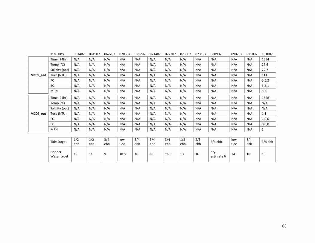
MMDDYY 061407 061907 062707 070507 071207 071407 072207 073007 073107 080907 090707 091007 101007

MC09_sed

Time (24hr) N/A N/A N/A N/A N/A N/A N/A N/A N/A N/A N/A N/A 1554

Temp (°C) N/A N/A N/A N/A N/A N/A N/A N/A N/A N/A N/A N/A 27.6

Salinity (ppt) N/A N/A N/A N/A N/A N/A N/A N/A N/A N/A N/A N/A 22.7

Turb (NTU) N/A N/A N/A N/A N/A N/A N/A N/A N/A N/A N/A N/A 111

FC N/A N/A N/A N/A N/A N/A N/A N/A N/A N/A N/A N/A 5,5,2

EC N/A N/A N/A N/A N/A N/A N/A N/A N/A N/A N/A N/A 5,5,1

MPN N/A N/A N/A N/A N/A N/A N/A N/A N/A N/A N/A N/A 500

MC09_out

Time (24hr) N/A N/A N/A N/A N/A N/A N/A N/A N/A N/A N/A N/A 1558

Temp (°C) N/A N/A N/A N/A N/A N/A N/A N/A N/A N/A N/A N/A N/A

Salinity (ppt) N/A N/A N/A N/A N/A N/A N/A N/A N/A N/A N/A N/A N/A

Turb (NTU) N/A N/A N/A N/A N/A N/A N/A N/A N/A N/A N/A N/A 1.1

FC N/A N/A N/A N/A N/A N/A N/A N/A N/A N/A N/A N/A 1,0,0

EC N/A N/A N/A N/A N/A N/A N/A N/A N/A N/A N/A N/A 0,0,0

MPN N/A N/A N/A N/A N/A N/A N/A N/A N/A N/A N/A N/A 2

Tide Stage

1/2 ebb

1/2 ebb

3/4 ebb

low tide

3/4 ebb

3/4 ebb

3/4 ebb

1/2 ebb

2/3 ebb

3/4 ebb low tide

3/4 ebb

3/4 ebb

Hooper Water Level

19 11 9 10.5 10 8.5 16.5 13 16 dry-estimate 6

14 10 13

63

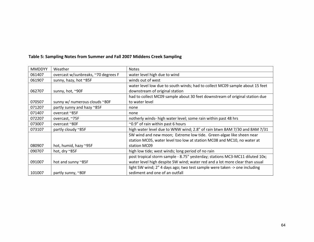
Table 5: Sampling Notes from Summer and Fall 2007 Middens Creek Sampling

MMDDYY Weather Notes

061407 overcast w/sunbreaks, ~70 degrees F water level high due to wind

061907 sunny, hazy, hot ~85F winds out of west

062707 sunny, hot, ~90F water level low due to south winds; had to collect MC09 sample about 15 feet downstream of original station

070507 sunny w/ numerous clouds ~80F had to collect MC09 sample about 30 feet downstream of original station due to water level

071207 partly sunny and hazy ~85F none

071407 overcast ~85F none

072207 overcast, ~75F notherly winds- high water level; some rain within past 48 hrs

073007 overcast ~80F ~0.9" of rain within past 6 hours

073107 partly cloudy ~85F high water level due to WNW wind; 2.8" of rain btwn 8AM 7/30 and 8AM 7/31

080907 hot, humid, hazy ~95F

SW wind and new moon; Extreme low tide. Green-algae like sheen near station MC05, water level too low at station MC08 and MC10, no water at station MC09

090707 hot, dry ~85F high low tide; west winds; long period of no rain

091007 hot and sunny ~85F post tropical storm sample - 8.75" yesterday; stations MC3-MC11 diluted 10x; water level high despite SW wind; water red and a lot more clear than usual

101007 partly sunny, ~80F light SW wind; 2" 4 days ago; two test sample were taken -> one including sediment and one of an outfall

64

Appendix:

Public Outreach Presentation: “Reversing Water Quality Declines: Recipes from Downeast”

65

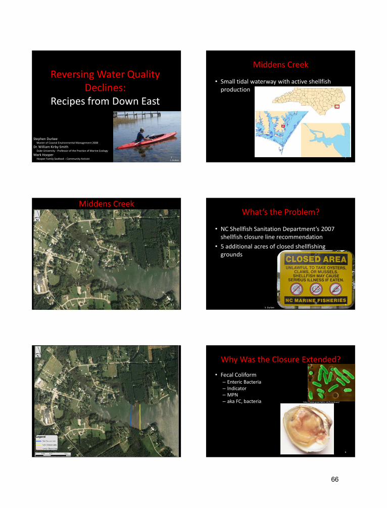
Reversing Water Quality Declines:

Recipes from Down East

Stephen DurkeeMaster of Coastal Environmental Management 2008

Dr. William Kirby-SmithDuke University - Professor of the Practice of Marine Ecology

Mark HooperHooper Family Seafood – Community Activist

S. Durkee

1

Middens Creek

• Small tidal waterway with active shellfish production

2

Middens Creek

3

What’s the Problem?

• NC Shellfish Sanitation Department’s 2007 shellfish closure line recommendation

• 5 additional acres of closed shellfishing grounds

S. Durkee4

5

Why Was the Closure Extended?

• Fecal Coliform– Enteric Bacteria– Indicator– MPN– aka FC, bacteria http://www.great-lakes.net/beachcast/

6

66

Why Was the Closure Extended?

• Fecal Coliform– Enteric Bacteria– Indicator– MPN– aka FC, bacteria

• Shellfish– Filter feeders– Collect and store fecal

coliform within tissue

• State Regulations– > 14 MPN = closure

http://www.great-lakes.net/beachcast/

7

Road Map to Recovery

1) Establish baseline fecal coliform characterization of Middens Creek

2) Explore potential statistical links between human development and fecal coliform levels

3) Public outreach

– Education

– Grassroots change

S. Durkee

8

9

Summer and Fall 2007 Sampling Results:

0

100

200

300

400

500

600

700

800

900

1000

MC01 MC02 MC03 MC04 MC05 MC06 MC07 MC08 MC09 MC10 MC10A MC11

1 429 22 32 38 47

255 242

2 038

Dry; n=7

MP

N

Sampling Station ID10

Summer and Fall 2007 Sampling Results:

0

100

200

300

400

500

600

700

800

900

1000

MC01 MC02 MC03 MC04 MC05 MC06 MC07 MC08 MC09 MC10 MC10A MC11

1 429 22 32 38 47

255 242

2 03844

144

292

226

500

894

465

922

620

369

714

922

Dry; n=7

Storm; n=3

MP

N

Sampling Station ID11

Stormwater

• Stormwater appears to be the most substantial factor

• Anything that speeds the delivery of stormwater to the waterway is contributing to the problem

• Within this problem lies the greatest potential for change!

– To be continued

http://www.enr.state.nc.us/upclose/images/where_stormwater_goes.jpg12

67

Historical Data

13

Historical Data

0

2

4

6

8

10

12

1998 1999 2000 2001 2002 2003 2004 2005 2006 2007 2008

FC by Year

MP

N

Year

14

Historical Data

0102030405060708090100

0

2

4

6

8

10

12

1998 1999 2000 2001 2002 2003 2004 2005 2006 2007 2008

FC by Year + Precipitation

MP

N

Year

Precip

itation

(")

15

Historical Data

• Historical Data in the context of human development

• First step is to define subwatershed

S. Durkee

16

17 18

68

19 20

0

100

200

300

400

500

600

700

Developed Parcels Undeveloped Parcels

234Acres

618Acres

Acr

es

234 developed acres / 107 houses = 2.2 acres per house

618 undeveloped acres / 2.2 acres per house = 281 houses

Middens Creek

21 22

Middens Creek

0

500

1000

1500

2000

2500

3000

3500

Undeveloped Developed

3448 m

2797 m

Met

ers

of

Sho

relin

e

2.1 miles

1.7 miles

23

Regression

y = 0.315x - 25.18R² = 0.800

0

2

4

6

8

10

12

75 85 95 105 115

Number of Houses Predicting FC1998-2006

Feca

l Co

lifo

rm

Number of Houses

-What does “Number of Houses” reflect?24

69

Historical Development

0

20

40

60

80

100

120

1700

1710

1720

1730

1740

1750

1760

1770

1780

1790

1800

1810

1820

1830

1840

1850

1860

1870

1880

1890

1900

1910

1920

1930

1940

1950

1960

1970

1980

1989

1999

Nu

mb

er o

f H

ou

ses

• Increasing at an increasing rate25

What’s the Government Doing?

• Federal

– Clean Water Act

• State

– Phase I and II

• Locally

– Coastal Stormwater rules

– CAMA

– Down East Conservation Ordinance

26

What Can We Do To Help?

1) Reduce fecal coliform sources

a) Regular septic tank maintenance

http://www.realtyresourceguide.com/septics/septic_tank3.gif

http://www.co.thurston.wa.us/health/ehoss/27

What Can We Do To Help?

1) Reduce fecal coliform sources

a) Regular septic tank maintenance

b) Pick up pet waste

http://www.dkimages.com/discover/previews/871/25028034.JPG28

What Can We Do To Help?

1) Reduce fecal coliform sourcesa) Regular septic tank maintenance

b) Pick up pet waste

c) Don’t encourage birds and wild animals

http://wdfw.wa.gov/wlm/living/graphics/raccon.jpghttp://www.pestproducts.com/images/canada-goose.JPG

http://upload.wikimedia.org/wikipedia/commons/thumb/

29

What Can We Do To Help?

2) Stop or slow the movement of stormwater into the water way

a) Rain gardens

http://www.urbanwaterquality.org/RainGardens/LIDRG1.jpg30

70

What Can We Do To Help?

2) Stop or slow the movement of stormwater into the water way

a) Rain gardens

b) Cisterns

http://www.fralo.net/images/productimages/cistern.gif 31

What Can We Do To Help?

2) Stop or slow the movement of stormwater into the water way

a) Rain gardens

b) Cisterns

c) Green roof

http://www.ncgreenbuilding.org/site/ncg/attachments/gallery_Groof7.jpg32

What Can We Do To Help?

2) Stop or slow the movement of stormwater into the water way

a) Rain gardens

b) Cisterns

c) Green roof

d) Vegetated buffers

S. Durkee

33

Vegetated Buffers

Pictures by S. Durkee

34

35

Vegetated Buffers

0

500

1000

1500

2000

2500

3000

3500

4000

0' Buffer 1'-19' Buffer 20'+ Buffer Bulkhead/Riprap

422 m

1400 m

3602 m

498 m

Met

ers

of

Sho

relin

e

0.26 miles

0.9 miles

2.2 miles

0.3 miles

36

71

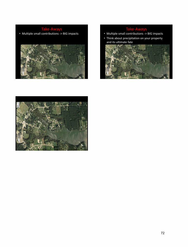
Take-Aways• Multiple small contributions -> BIG impacts

37

Take-Aways• Multiple small contributions -> BIG impacts

• Think about precipitation on your property and its ultimate fate

38

39

72