community and gradient analysis: matrix approaches in macroecology the world comes in fragments

Nicolaus Copernicus University – Department of Animal Ecology

Community and gradient analysis: Matrix approaches in macroecology

The world comes in fragments

Statistical inference means to compare your hypothesis H1 with an appropriate null hypothesis H0.

Hypothesis correct

1-

1-

Hypothesis wrong

Hypothesis rejected

Hypothesis accepted

Type I error

Type II error

Simple examples in ecology are

• The correlation between species richness and area

(H0: no correlation, t-test)

• Differences in productivity between plots of different soil properties.

(H0: no difference between means, ANOVA)

But what about more complex patterns:

• Relative abundance distributions

• Productivity – diversity relationship

• Succession

• Community assembly

Galapagos Islands n

i ii 1

H p ln p

Var(H) Jackknife[Samp(H)]

But: Your variance estimator comes from the underlying distribution of species and individuals.

Does the variance stem from • Species interactions?• Random processes?• Evolutionary history?• Ecological history?

In fact we do not have an appropriate null hypothesis.

Bootstrapped or jackknifed variance estimators only catch the variability in the underlying distribution.

We compare diversities on islands

A t-test points to significant differences in diversity.

http://upload.wikimedia.org/wikipedia/commons/0/09/Shannon_2.jpeg

Statistical inference

Species lip kor helPterostichus melanarius 704 1199 169Pterostichus oblongopunctatus (Fabricius) 180 1019 8Platynus assimilis (Paykull) 117 76 9Carabus granulatus 113 154 11Nebria brevicolis (Fabricius) 94 34 0Harpalus 4-punctatus Dejean 69 555 67Patrobus atrorufus (Stroem) 37 11 0Pterostichus strennus (Panzer) 24 28 6Epaphius secalis (Paykull) 8 0 0Badister bullatus (Schrank) 7 0 1Oxypselaphus obscurus (Herbst) 7 96 0Notiophilus palustris (Duftshmid) 7 4 2Synuchus vivalis (Illiger) 5 4 10Carabus nemoralis Muller 5 10 16Amara plebeja (Gyllenhal) 4 0 0Leistus terminatus (Hellwig) 4 3 1Badister unipustulatus Bonelli 3 0 0Leistus rufomarginatus (Duftshmid) 3 0 3Pterostichus nigrita (Paykull) 2 0 0Poecilus versicolor (Sturm) 2 0 0Pseudoophonus rufipes (De Geer) 2 90 3Harpalus latus (Linnaeus) 2 1 0Pterostichus antracinus 2 2 11Notiophilus biguttatus (Fabricius) 2 0 1Stomis pumicatus (Panzer) 2 14 2Amara brunea (Gyllenhal) 1 0 3

Is species co-occurrence random or do species have

similar habitat requirements?

A simple regression analysis points to joint occurrences.

PF(r=0) < 0.00001

)2(1 2

2

nRR

F

Abundance scale exponentially. Extreme values bias the results

Spearman’s r = 0.67, PF(r=0) < 0.001

Classical Fisherian testing relies on an equiprobable null assumption. All values are equiprobable.

In ecology this assumption is often not realistic.

y = 1.8589x + 26.397R² = 0.7075

0

500

1000

1500

0 500 1000

kor

lip

Species lip kor helPterostichus melanarius 704 1199 169Pterostichus oblongopunctatus (Fabricius) 180 1019 8Platynus assimilis (Paykull) 117 76 9Carabus granulatus 113 154 11Nebria brevicolis (Fabricius) 94 34 0Harpalus 4-punctatus Dejean 69 555 67Patrobus atrorufus (Stroem) 37 11 0Pterostichus strennus (Panzer) 24 28 6Epaphius secalis (Paykull) 8 0 0Badister bullatus (Schrank) 7 0 1Oxypselaphus obscurus (Herbst) 7 96 0Notiophilus palustris (Duftshmid) 7 4 2Synuchus vivalis (Illiger) 5 4 10Carabus nemoralis Muller 5 10 16Amara plebeja (Gyllenhal) 4 0 0Leistus terminatus (Hellwig) 4 3 1Badister unipustulatus Bonelli 3 0 0Leistus rufomarginatus (Duftshmid) 3 0 3Pterostichus nigrita (Paykull) 2 0 0Poecilus versicolor (Sturm) 2 0 0Pseudoophonus rufipes (De Geer) 2 90 3Harpalus latus (Linnaeus) 2 1 0Pterostichus antracinus 2 2 11Notiophilus biguttatus (Fabricius) 2 0 1Stomis pumicatus (Panzer) 2 14 2Amara brunea (Gyllenhal) 1 0 3

Species do not have the same abundances in the meta-

community and sites differ in capacity.

Statistical testing should incorporate such differences in

occurrence pobabilities.Ecologists often have a good H1

hypothesis.Much discussion is about the

appropriate null assumption H0.

What do we expect if colonization of these

three islands is random?

Ecology is interested in the differences between observed pattern and random expectation.

Our statistical tests should deal with these differences and not with raw pattern!

If we use classical Fisherian testing nearly all empirical ecological matrices are significantly non-random.

Thus we can’t separate ecological interactions from mass effects.

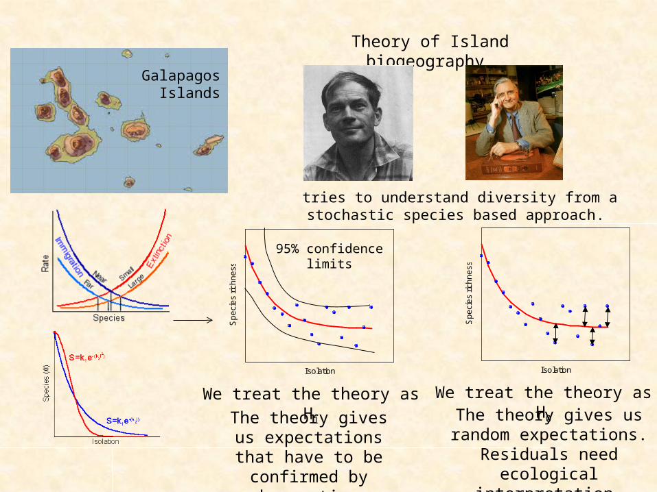
Theory of Island biogeography

Galapagos Islands

tries to understand diversity from a stochastic species based approach.

We treat the theory as H1

The theory gives us expectations that have

to be confirmed by observation.

Isolation

Sp

eci

es

rich

ne

ss

z

Isolation

Sp

eci

es

rich

ne

ss

z95% confidence limits

We treat the theory as H0

The theory gives us random expectations.

Residuals need ecological interpretation.

http://upload.wikimedia.org/wikipedia/en/a/a9/Edward_O_Wilson.jpg

Multispecies metapopulation and patch occupancy models

Islands in a fragmented landscape

Random dispersal of individuals

between islands results in a

stable pattern of colonization

ijd

ij j i i

i, j i

dp am (e A p ) 1 p p

dt A

The change of occupancy p in time depends on

patch size and distance according to a logistc

growth equation.

Metapopulation models are single

species equivalents of the island

biogeography model.

Multispecies metapopulation models

give null expectations on community structure.

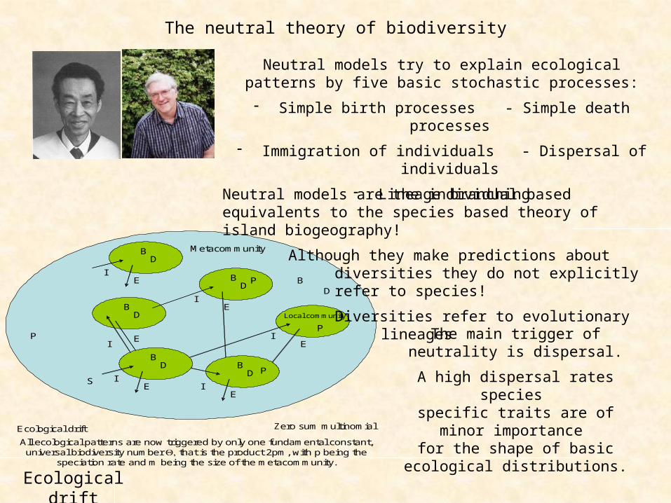
The neutral theory of biodiversity

EI

S

All ecological patterns are now triggered by only one fundamental constant, universal biodiversity number that is the product 2pm, with p being the

speciation rate and m being the size of the metacommunity.

Metacommunity

BD

EI

BD

EI

BD

EI

BD

EI

BD

EI

BD

P

P

P

P

Local community

Ecological drift Zero sum multinomial

Neutral models try to explain ecological patterns by five basic stochastic processes:

- Simple birth processes - Simple death processes

- Immigration of individuals - Dispersal of individuals

- Lineage branching

Neutral models are the individual based equivalents to the species based theory of island biogeography!

Although they make predictions about diversities they do not explicitly refer to species!

Diversities refer to evolutionary lineages

Ecological drift

The main trigger of neutrality is dispersal.

A high dispersal rates species specific traits are of minor importance

for the shape of basic ecological distributions.

Used as H1 Neutral models make explicit predictions about

Shape and parameters of species rank order distributions

Species – area relationships

Abundance - range size relations

Local diversity patterns

Patterns of succession

Local and regional species numbers

Branching patterns of taxonomic lineages

Used as H0 residuals from model predictions are measure of ecological interactions

• The model contains a number of hidden variables (dispersion limitation, branching

mode, dispersal probability, isolation, matrix shape…

• CPU times are a limiting resource

• Variable carrying capacities are needed to obtain realistic evolutionary time scales

Birth / Death

Dispersal limitation function

Dispersal rate

Mode and frequency of speciation

Immigration rate

Carrying capacities

The neutral, metapopulation and island biogeography models contain too many hidden variables to be of use as null hypothesis.

Ecological realism without too many parameters

We need null models that are ecologically realistic and rely on few assumptions that

apply to all species.

Gradient of null model assumptions including more and more constraints.

Null models only use information given in the matrix. Theses are matrix fill, marginal totals, and degree distributons.


Retain fill Retain fill and row totals

Retain fill and column totals

Retain fill and row degree distribution

Retain fill and column degree

distribution

Retain fill and row and

column degree distribution

Retain row and column totals

Possible constraints

Rows

Columns equiprobableproportional to marginal

totals

Marginal totals fixed

equiprobable x x xproportional to marginal totals x x x

marginal totals fixed x x x

S 4 2 7 1 3 5 6 8 S

8 1 1 0 0 0 1 1 1 53 1 1 0 0 1 0 1 0 49 1 1 1 0 0 1 0 0 41 1 0 0 1 0 0 0 1 32 0 0 1 1 0 0 1 0 36 0 0 1 0 1 1 0 0 34 0 1 0 0 1 0 0 0 2

10 0 0 1 1 0 0 0 0 25 1 0 0 0 0 0 0 0 17 0 0 0 0 0 0 0 1 1

S 5 4 4 3 3 3 3 3

Degree distribution

Marginal totals

Start from an empty matric and fill it

randomly without or according to some

constraints


Equiprobable - equiprobable

Proportional - proportional

Equiprobable - fixed

Fixed - Equiprobable

Fixed - proportional

Fixed - fixed

Includes mass effects

Most liberal

Identifies nearly all empirical

matrices as being not random

Low discrimination

power

Partly includes mass effects

Appropriate if species

abundances or site capacities

are equal

Identifies most empirical


Partly excludes mass effects

Appropriate if species

abundances or site capacities are

proportional to metapopulation abundances or sites capacities

Identifies many empirical


Excludes most mass effects

Appropriate if column totals

are proportional to sites capacities

Identifies many empirical

matrices as being random

Excludes mass effects

Appropriate if nothing is

known about abundances

and capacities

Identifies most empirical

matrices as being random

SitesSpecies 1 2 3 4 5 6 7 8A 1 1 1 0 0 0 0 1B 1 1 1 1 1 1 1 0C 1 1 1 1 1 1 1 1D 1 1 1 1 1 1 1 1E 1 1 0 1 0 0 1 1F 1 1 1 1 1 1 1 1G 1 0 1 1 1 0 0 0H 1 1 1 0 0 1 1 1I 0 1 1 0 1 0 0 1J 1 1 1 1 1 1 1 1K 0 1 1 1 1 0 0 1L 1 1 0 0 0 1 1 0

1 0 0 10 1 1 0



An initial empty matrix is filled step by step at random. If after a

placement violates the above constraints it steps back and places elsewhere. The process continues until all occurrences are placed.

Major drawbacks:

Long computation times

Potential dead ends

Fill algorithm

Swap algorithm

The algorithm screens the original matrix for

checkerboards and swaps them to leave row and columns sums

constant. Use at least 10*species*sites swaps.

Major drawbacks:

Generates biased matrices in dependence

on the original distribution

The algorithm starts with a random matrix according to the row and column constraints and

sequentially swaps all 2x2 submatrices until only 1 and 0

remain.

Major drawbacks:

Randomized matrices have a low variance

that are prone to type II errors.

Trial algorithm(Sum of squares reduction)


2 0 1 10 1 1 0

Algorithms for the fixed fixed null model


1 0 0 10 1 1 0

The Swap algorithm is most often used

1. Sequential swap: First make a burn in and swap 30000 times and then use each further 5000 swaps as a new random matrix

2. Independent swap: Generate each random matrix from the original matrix using at least 10*species*sites swaps.

Compare the observed metric scores with the simulated ones (100 or more randomized matrices)

638.0141.0

711.3621.3 sxx

scoreZ

Z-scorelower CL = -0.37

Z-scoreupper CL = -3.00

0

500

1000

1500

2000

3.57 3.67 3.78 3.89 3.99 4.1Scores

Fre

quen

cy

Observed score

upper CLLower CL

Using abundances

Abundance

Species

Populations

equiprobable

proportional to

observed totals

marginal totals fixed

proportional to marginal

totals

equiprobable

marginal totals fixed

proportional to marginal totals

equiprobable

populations fixed

Including abundances into null models increases the number of possible null models

These 27 combinations regard rows, columns, and row and columns.

CA

SA

AA

MA

U

Mantel

IA

IT

ITC

ITR

IS

ISC

ISR

IR

IF

OA

OF

PM

PR

PC

CA

SA

AA

MA

U

Mantel

200 MS200 MR

X

IA

IT

ITC

ITR

X

CA

SA

AA

MA

U

Mantel

200 MR

IA

IT

ITC

ITR

X

Dependence on size, fill, abundance

CA

SA

AA

MA

U

Mantel

Mmod = 600 seeded MR

IA

IT

ITC

ITR

X

BR

CASAMAU

IT

185 empirical abundance matrices

Dependence on null matrix

constructionPower to detect

segregation

Mmod = 200 seeded MR

Power to detectaggregation

XTest for differencesbetween taxa and

biomeC-score

Fixed -fixed null

model

185 empirical matrices transformed to presence – absence matrices

XTest for differencesbetween taxa and

biome

CA Morisita Variance Mantel

LCL UCL LCL UCL LCL UCL LCL UCL

Prop-prob, total abundance fixed 0 39 5 8 3 2 0 0

Prop-prob , row/column abundances fixed 20 1 0 21 2 20 0 0

Prop– prop, row/column richenss fixed 43 25 0 39 0 98 0 2

Prop-prob, total richnes fixed 65 6 91 0 73 4 49 0

Row/column richenss and abundance fixed 8 11 25 12 3 45 0 0

Occurences fixed 58 2 5 48 2 17 0 166

Occurrences and row/cloumn abundances fixed 0 72 8 24 20 56 0 164

Populations fixed 182 3 0 194 0 196 0 158

Populations per column fixed 171 1 1 145 1 181 15 142

Populations per row fixed 180 1 0 193 0 193 0 158

Testing of null models and metrics using proportional random matrices. The metrics shouldn’t detect these matrices as being non-random.

200 random matrices

0 0.2 0.4 0.6 0.8 1

Interaction

Arthropods

Carabidae

Non-arthropod invertebrates

Plants

Vertebrates

C-Score

Abundance matrices are more often detected as being non-random

0 0.2 0.4 0.6 0.8 1

Interaction

Arthropods

Carabidae

Non-arthropod invertebrates

Plants

VertebratesCA

),,,(),,,(; cdbdcabacdbdcabadc

ba

ST

4CACA

m(m 1)n(n 1)

)1(

))((2,

SS

NNNN

CS jiijjiji

Fraction of 185 matrices detected as being significantly (two-sided 95% CL) segregated (dark bars) or aggregated (white bars).

community and gradient analysis: matrix approaches in macroecology the world comes in fragments

Documents

stochastic species

species cooccurrence

species interactions

appropriate null hypothesis

appropriate null assumption

species richness

random expectations

area h