communications impact of hall effect plasma
TRANSCRIPT

COMMUNICATIONS IMPACT OF HALL
EFFECT PLASMA THRUSTERS
by
JAMES CLAUDE DICKENS, B.S.E.E., M.S.E.E
A DISSERTATION
IN
ELECTRICAL ENGINEERING
Submitted to the Graduate Faculty of Texas Tech University in
Partial Fulfillment of the Requirements for
the Degree of
DOCTOR OF PHILOSOPHY
Approved
Co-;^hairperson of th§ Committee
Co-C/ha/roerson of the Committee
Accepted
Dean of the Graduate School
May, 1995

J
T 3 ^ ACKNOWLEDGMENTS • ^ '* >z
([ I would like to express my appreciation to Dr. M. Kristiansen and Dr E.
O'Hair for their support and technical advice during this research project. I would
also like to thank the other members of my committee, Dr L. Hatfield, Dr. T. Trost,
and Dr. F. Curran for their guidance. I am also gratefijl to John Mankowski, for his
assistance in designing and building hardware necessary to complete the project.
I am especially indebted to J. Sankovic, E. Pencil, T. Haag, and D. Manzella,
who have provided many insights and assistance in completing this project. In
addition, without the use of NASA LeRC's vacuum tank facilities and equipment,
none of this work would be possible,
Finally, I would like to thank my family and especially my wife, Molly, who has
provided support and encouragement throughout my academic career.
11
T.^BLE OF CONTENTS
ACKNOWLEDGMENTS ii
ABSTRACT iv
LIST OF TABLES v
LIST OF FIGURES vi
CHAPTER
1. INTRODUCTION 1
2. PROBLEM DESCRIPTION 5
3. PLUME MODEL 9
4. MICROWA\^ INTERFEROMETER 22
5. PHASE SHIFT MEASUREMENTS 27
6. PHASE NOISE 48
7. CONCLUSIONS 60
REFERENCES 65
APPENTDIX
A. LANGMUIR PROBE PLOTS 67
B. MATHCAD WORKSHEETS 74
C PHASE SHIFT PLOTS 77
D. POWER SPECTRAL DENSITY PLOTS 85
111

ABSTRACT
A Hall effect thruster is an electric space propulsion device, in which a gas
(typically Xenon) is ionized and accelerated by a self-induced electric field. Because
the exhaust plume of a Hall effect thruster is an ionized gas, the thruster's plume can
affect the propagation of electromagnetic radiation. These effects could have a
significant impact on the channel capacity of satellite communication systems.
The first part of the study was devoted to developing a far field plume model
that can predict both the spatial and temporal number density in the plume of three
different Hall effect thrusters. The spatial dependence of the number density in the
plume was determined using a swept Langmuir probe. The temporal dependence was
determined using a high speed Langmuir probe positioned along the centerline of the
plume.
In an effort to verify the far field number density plume model, a sampling
microwave interferometer was developed, that can accurately measure the phase shift
of microwave signals propagating through the plume of a Hall effect thruster. The
interferometer was used to measure the phase shift of a 6 GHz microwave signal
during the startup of a Hall effect thruster with several different propagation paths A
comparison between the model predicted phase shift and the experimentally obtained
phase shift are made. A microwave spectrum analyzer was used to qualify and
quantify the plumes effect on the phase noise of a microwave signal propagating
through the plume.
IV

LIST OF TABLES
3.1. Plume model coefficients 1
A. 1. Operating parameters of the thrusters for the Langmuir probe and current plots in Appendix A 68
C 1 . Operating parameters of the thrusters for the phase shift plots and current waveforms in Appendix C 78
D. 1. Operating parameters of the thrusters for the power spectral density plots and current waveforms in Appendix D 86
V

LIST OF FIGURES
1.1. Cross-section diagram of a TAL plasma thruster 1
1.2. Cross-section diagram of a TML plasma thruster 2
3.1. Normalized number density profile of a D-55 thruster 11
3.2. Normalized number density profile of a SPT-100 thruster 11
3.3. Comparison of the measured plume profile of a D-55 thruster and the plume model of Equation (3,2) 13
3.4, Comparison of the measured plume profile of an SPT-100 thruster and the plume model of Equation (3,1) 14
3.5, Percent number density for a T-100 thruster 16
3.6, Percent peak current waveform for a T-100 thruster 16
3.7, Percent number density for an SPT-100 thruster 17
3.8. Percent peak current waveform for an SPT-100 thruster 17
3.9 Percent number density of a D-55 thruster 17
3.10. Percent peak current waveform of a D-55 thruster 18
3.11. FFT of the D-55 number density waveform 19
3.12. FFT oftheT-lOOnumber density waveform 20
3.13. Plot of the static plume model for an SPT-100 21
3.14. Plot of the complete plume model for an SPT-100 21
4.1. Schematic diagram of a basic microwave interferometer 23
4.2. Block diagram of a sampling microwave interferometer 24
5.1. Sketch of parallel propagation path (relative to the exit plane) 28
5.2. Parallel start-up phase shift at 0.5 m for a T-lOO 28
\i

5.3. Perpendicular start-up phase shift at 0,9 m for an SPT-100 :, 30
5.4. Perpendicular start-up phase shift at 0.9 m for a D-55 30
5.5. Sketch of 45 deg propagation path 31
5.6. Startup phase shift along a 45 deg propagation path for a D-55 32
5.7. Startup phase shift along a 45 deg propagation path for an SPT-100 33
5.8. Startup phase shift along a propagation path perpendicular to the exit plane of a D-55 33
5.9. Startup phase shift along a diagonal propagation path for an end-of-life SPT-100 ^ 35
5.10. Change in phase shift due to change in cathode flow rate for a D-55 (0.2mg/s at 2 sec linearly to 1,6 mg/s at 28 sec) 36
5.11. Measured phase transients of a 6 GHz signal propagating along a parallel
path (relative to the exit plane) through the plume of a T-100 37
5 12, Current waveform of the T-100 in Fieure 5,11 38
5 13 Predicted phase shift along a parallel propagation path 0.5 m down from the exit plane as a fianction of m, for the T-100 38
5.14. Measured phase transients of a 6 GHz signal propagating along a parallel propagation path through the plume of a SPT-100 40
5.15. Current waveform of the SPT-100 in Figure 5.14 40
5.16. Predicted phase transients of a 6 GHz signal along a parallel propagation path 0.9 m down from the exit plane as a function of m 40
5.17. Measured phase transients of a 6 GHz signal propagating along a 45 deg diagonal propagation path for a SPT-100 42
5.18. Current waveform of the SPT-100 in Figure 5.17 42
5.19. Predicted phase transients along 45 deg diagonal propagation path at 1 m down from the exit plane as a fijnction of m 42
VI1
5.20. Measured phase transients of a 6 GHz signal propagating along the parallel propagation path through the plume of a D-55 44
5.21. Current waveform of the D-55 in Figure 5.20 44
5.22. Measured phase transients of a 6 GHz signal propagating along a 45 deg diagonal propagation path for a D-55 44
5.23. Current waveform for Figure 5.22 45
5.24. Measured phase transients of a 6 GHz signal propagating along a 31 deg propagation path for an end-of-life SPT-100 45
5.25. Current waveform for Figure 5,24 45
5.26. Predicted phase transients along 31 deg diagonal propagation path at
1.8 m to the side of an SPT-100 as a fijnction of m 46
6.1. Phase noise test setup 50
6.2. Spectrum of a received signal with and without a T-lOO running
(1 MHz span) 51
6.3. Current waveform of the T-lOO in Figure 6.2 51
6.4. Spectrum of a received signal with and without an SPT-100 running
(200 kHz span) 52
6.5 Current waveform of the SPT-100 in Figure 6.4 52
6.6. Spectrum of a received signal with and without a D-55 running
(200 kHz span) 53
6.7. Current waveform of the D-55 in Figure 6.6 54
6.8. Spectrum of a received signal with and without a SPT-100 running along
the 45 deg diagonal propagation path(100 kHz span) 55
6.9. Current waveforms of the SPT-100 in Figure 6.8 55
6.10. Spectrum of a received signal along the 45 deg diagonal propagation path with a D-55 operating at 3.5 A and 4,5 A (200 kHz span) 56
6.11. Current waveforms of the D-55 in Figure 6,10 56 viii

6.12, Spectrum of a 6 GHz received signal with and without an end-of-life SPT-100 running (200 kHz span) 58
6.13, Current waveform of the end-of-life SPT-100 in Figure 6,12 58
6.14, Spectrum of a 2.8 GHz received signal with and without an end-of-life SPT-100 running (750 kHz span) 59
7.1. Phasor illustration of thruster induced phase noise and typical additive
noise 62
A.l. Percent number density of a T-lOO ( file: lang205 ) 69
A.2. Percent peak current of a T-lOO ( file: curr205 ) 69
A.3. Percent number density of a T-lOO ( file: lang202 ) 69
A,4. Percent peak current of a T-lOO ( file: curr202 ) 70
A. 5. Percent number density of a T-100 ( file: lang204 ) 70
A.6. Percent peak current of a T-lOO ( file; curr204 ) 70
A. 7. Percent number density of an SPT-100 ( file: lang526 ) 71
A. 8. Percent peak current of an SPT-100 ( file: curr526 ) 71
A.9. Percent number density of an SPT-100 ( file: lang522 ) 71
A.IO. Percent peak current of an SPT-100 ( file: curr522 ) 72
A l l . Percent number density of a D-55 (file: lang404 ) 72
A.12. Percent peak current of aD-55 ( file: curr404 ) 72
A.13. Percent number density of aD-55 (file: lang406 ) 73
A.14. Percent peak current of a D-55 (file: curr406 ) 73
C I . Start-up phase shift (along a parallel path at 0.5 m) for a T-lOO (file phasll6) 79
C.2. Current waveform of the T-lOO for Figure CI 79
IX

C,3 Phase shift of a 6 GHz passing through the plume of a T-100 ( parallel
path 0,5 m from the exit, file: phasl07) 79
C.4. Current waveform of the T-lOO for Figure C.3 80
C.5. Start-up phase shift (along a 45 deg diagonal path) for an SPT-100 (file phas614) 80
C.6. Current waveform of the SPT-100 for Figure C 5 80
C.7. Phase shift of a 6 GHz passing through the plume of an SPT-100 along a
45 deg diagonal path (file: phas613) 81
C.8. Current waveform of the SPT-100 for Figure C.7 81
C.9. Phase shift of a 6 GHz passing through the plume of an SPT-100 along a
45 deg diagonal path (file: phas612) 81
CIO, Current waveform of the SPT-100 for Figure C,9 82
C11. Start-up phase shift (along a 45 deg diagonal path) for a D-55
(filephas714) 82
C.12. Current waveform of the D-55 forFigureC.il 82
C.13. Phase shift of a 6 GHz passing through the plume of a D-55 along a 45
deg diagonal path (file: phas707) 83
C.14. Current waveform of the D-55 for Figure C.13 83
C.15. Phase shift of a 6 GHz passing through the plume of aD-55 along a 45
deg diagonal path (file: phas710) 83
C.16. Current waveform of the D-55 for Figure C.15 84
C17. Phase shift of a 6 GHz passing through the plume of a D-55 along a 45 deg diagonal path (file: phas713) 84
C.18. Current waveform ofthe D-55 for Figure C17 84 D. 1. Power spectral density of a 3.8 GHz signal with a parallel path 1 m down
stream from the exit of an SPT-100 (200 kHz span, file: an021) 87 D.2. Current waveform ofthe SPT-100 for Figure D.l 87
x

D,3. Power spectral density of a 6 GHz signal with a parallel path 1 m down stream from the exit of an SPT-100 (200 kHz span, file; an026) 87
D 4. Current waveform ofthe SPT-100 for Figure D.3 88
D.5. Power spectral density of a 6 GHz signal with a 45 deg diagonal path
through the plume of an SPT-100 (200 kHz span, file: an022) 88
D.6. Current waveform of the SPT-100 for Figure D. 5 88
D.7. Power spectral density of a 6 GHz signal with a 45 deg diagonal path through the plume of an SPT-100 (750 kHz span, file: an629) 89
D.8. Current waveform ofthe SPT-100 for Figure D.7 89
D.9. Power spectral density of a 6 GHz signal phase modulated with a 200 kHz tone propagating through the plume of an SPT-100 along a 45 deg diagonal path (750 kHz span, file: an632) 89
D 10. Current waveform ofthe SPT-100 for Figure D,9 90
D. 11. Power spectral density of a 6 GHz signal with a parallel path 1 m down
stream from the exit of aD-55 (200 kHz span, file: anOllb) 90
D,12, Current waveform ofthe D-55 for Figure D,l 1 90
D,13. Power spectral density of a 3.8 GHz signal with a parallel path 1 m down
stream from the exit of a D-55 (1 MHz span, file: an017b) 91
D.l 4 Current waveform ofthe D-55 for Figure D.l 3 91
D. 15. Power spectral density of a 6 GHz signal with a 45 deg diagonal path through the plume of a D-55 (750 kHz span, file: an636) 91
D.16. Current waveform ofthe D-55 for Figure D.15 92 D. 17 Power spectral density of a 6 GHz signal phase modulated with a 50 kHz
tone propagating through the plume of a D-55 along a 45 deg diagonal path (750 kHz span, file: an638k) 92
D.l 8. Current waveform ofthe D-55 for Figure D.l 5 92
xi

CHAPTER 1
INTRODUCTION
Hall thrusters are a type of electric space propulsion unit in which a gas
(typically Xenon) is ionized and accelerated by a self-induced electric field. There are
two main types of Hall thrusters currently being investigated, the thruster with
magnetic layer (TML) and the thruster with anode layer (TAL). Although the TML
and the TAL are structurally different, their theory of operation is the same. Both
types of Hall thrusters have four major components, an inner magnetic coil, an outer
magnetic coil, an anode/gas ejector, and a cathode assembly. In addition, the TML
has an insulator lining the discharge chamber. Cross-section diagrams ofthe TAL and
TML are shown in Figure 1 1 and Figure 1.2, respectively.
Cathode Assembly
H / / ^ • I ' 5
Annular Anode
Xenon Gas Feed Lines -
Main Body Housing —' and Primars' Pole Piece
Insulator
/ / • / / / /
/ / ,• ./-l'
5?;^ - Magnetic Field Profiler '— Inner Magnetic Coil
\ /
• — Outer Magnetic Coil
Figure 1.1. Cross-section diagram of a TAL plasma thruster.
1

Cathode Assembly
V Xenon Gas Feed Lines —
Main Bod)- Housing —-" and Pnman Pole Piece
'' / /A"—' ' 'r'—r'-^— : ' > > \ V — > • • ••'
A ///'/// '/^/, 'y '• / - /y W ' X '/ '/ /, /'
KM . ^ • ^
Annular Insulator
^
/ y
'/•/y'y'//' ^yV//^''y' '?. ' / y / / /
/ / / / / / / / / y ' y ' -
/ / / ' • '^ y / , / y / / , / ' • y / y y ' y ' ,\
-Magnetic Field Profiler Inner Magnetic Coil
Insulator
Anode
y /
• / y / ' y / , ,
• / , '
y ' \
— Outer Magnetic Coil
Figure 1,2, Cross-section of a TML plasma thruster.
The cathode assembly is used as a source of free electrons to neutralize the
plasma exhaust plume and to provide electrons to the acceleration and ionization
regions in the discharge chamber. The inner and outer magnetic coils are biased with a
dc current to produce a radial magnetic field. When a voltage is applied across
cathode to anode, the electrons being emitted by the cathode assembly are swept
toward the anode. The radial magnetic field lines "trap" the free electrons and impede
their motion from the cathode to the anode and thus produce a cyclotron motion along
equipotential magnetic field lines. The Xenon gas, introduced through the anode,
difiFuses into the discharge and into an ionization region where the "trapped" electrons
collide with the Xenon atoms, exciting the atoms into an ionized state (preferably a

singly ionized state). The Xenon ions are then accelerated axially by the electric field
produced by the trapped electrons. When an electron collides with a Xenon atom, the
electron diffuses towards the anode, thus after a finite number of collisions, the
electron reaches the anode and must be replaced by additional electrons from the
cathode assembly to continue the process
The ceramic insulator lining the wall ofthe main discharge chamber in the
TML is utilized to prevent erosion ofthe magnetic pole pieces. The TAL relies upon
the magnetic field profile to prevent pole piece erosion The TML magnetic field
profile is broader than that ofthe TAL and has a peak value located within the thruster
body The area of acceleration is located in the area of peak magnetic field, thus for
the TML, the acceleration region is also contained within the thruster body In
contrast, the TAL has a sharp magnetic field profile with a peak value at the exit plane.
As a resuh the acceleration region for the T.AL is located at the exit ofthe thruster,
therefore, eliminating the need for a ceramic insulator
The performance of TML and TAL thrusters ofthe same electric power, has
been shown by Sankovic [1,2] and Garner [3] to be ver}' similar. Typical xalues of
specific impulse (ISP) for a 1,5 kW Hall effect thruster are in the range of 1500 s to
1800 s and they have an efficiency that can exceed 50 percent. In particular, three
1.35 kW Hall effect plasma thrusters have been characterized and will be the subject of
this research report. The single TAL thruster tested is the D-55 manufactured by
TSNIIMASH (Research Institute of Machine Building) in Russia, The two TML
thrusters tested are the SPT-100, manufactured by Fakel Enterprises and the T-lOO,

manufactured by the Scientific Research Institute for Thermal Process (NTITP), Both
of these thrusters are also manufactured in Russia
The first chapter of this paper discusses the potential impacts of Hall effect
thrusters on communication systems In the second chapter, a spatial and temporal
far-field plume model is developed. Chapter 3 describes a sampling microwave
interferometer developed to provide a way to verify the plume model and to quantify
the magnitude and frequency of phase oscillations and phase transients experienced by
communications signals propagating through the plume of Hall effect thrusters. In
Chapter 4, the experimentally obtained phase shift data is presented and discussed.
Chapter 5 describes an experiment used to determine the impact a Hall effect
thruster's plume can have on the phase noise of a communication signal. The results
of this experiment are also presented in that chapter The final chapter presents
conclusions that can be made from the research and recommendations to minimize the
thruster's impact on communication systems. In addition, suggestions for fijture work
are also discussed.

CHAPTER 2
PROBLEM DESCRIPTION
Potential applications for Hall effect thrusters include North-South station
keeping and orbit raising of communications satellites, deep space research missions,
and general positioning of military satellites. Because each of these applications
involves extensive data transfer between the satellite and a ground station or another
space vehicle, the adverse effects ofthe propulsion system on communications must be
characterized and minimized. Areas of potential impact include radiated EMI, signal
attenuation, beam aberrations, increased phase noise, and high-speed phase transients.
The scope of research presented in this paper is limited to the latter ofthe two impact
areas, increased phase noise and high-speed phase transients.
Satellite communication systems can utilize any one of several modulation
methods, including frequency-shift keying (FSK), phase-shift keying (PSK), multistate
frequency-shift keying (M-ary FSK), and muhistate phase-shift keying (M-ary PSK).
Each of these modulation schemes transmits information in the phase or frequency of a
RF carrier signal. Frequency bands typically allocated to communication satellites are
in the microwave range of 4 GHz and 6 GHz. Because satellite communication
systems must transmit hundreds of signals at a time utilizing either time division
multiplexing or frequency muhiplexing, any increase in phase noise or phase transients
can cause channel cross-talk in analog systems or increased bit error rates in digital

systems [4,5]. The resuh of either of these situations is a loss in channel capacity and,
therefore, an economic loss to the satellite owner.
The plume of a Hall effect thruster is composed primarily of ionized Xenon
atoms and an equal number of free electrons, thus forming a neutral plasma.
Therefore, to determine how the exhaust plume can impact communications, the
interaction between the plasma and a microwave signal must be examined. A long
known effect of free electrons in a plasma is the effect on the relative dielectric
constant and thus the local wavenumber The local wavenumber in the plasma, k, can
be expressed as.
k{x,y,z) = ^<^o^ -o)Ax,y,z)
(21)
where cOo is the carrier frequency and c is the speed of light. The local plasma
frequency cOp is given by.
coAx,y,z) = \n^{x,y,z)q-
^o^h (2,2)
where q is the charge of an electron, me is the mass of an electron and ne is the local
plasma electron number density. The phase difference between waves traveling along
a path with a plasma present and one without a plasma present can be expressed as.
^e=\[k,-k{x,yr^)\ix^k^\ 1-Jl n^{x,y,z)q'
^o ^o^h dX, (2.3)
where the integral is along the signal propagation path, ko is the wavenumber in free
space, and 8o is the permitti\'ity in free space. The phase shift expressed in Equation

(2.3) is static and does not represent a serious communication problem. If the local
number density, n^ is not temporally stable however, a modified phase shift equation is
given by.
Aeit) = k^j ^o £o^h
1_ | l _ ! ! i l M i l i i V ^ ^ (2.4)
In this equation, the phase shift is a fijnction of time due to the temporal dependence
ofthe local number density, n .
In a communication system using phase modulation, the transmitted signal can
be expressed as,
f{t), = Acos{(oJ^y{t)) (2.5)
where A is the amplitude, cOc is the carrier frequency, and y(t) is the time dependent
information to be transmitted. If the transmitted signal has a propagation path that
passes through a region of time-vary'ing plasma, the received signal will be modified
and have a form given by,
/ ( / ) , =/icos(^,/ + r(?) + A^(0) (2,6)
At the receiver end ofthe communication link, the extracted phase information will
contain the original information signal, Y(t), plus the additive phase shift signal, A9(t),
Because A9(t) is unknown and possibly random, extraction ofthe function from the
original signal is impossible and thus must be treated as an additive noise term. In a
similar analysis, it can be shown that a frequency modulated signal passing through a
7

temporally unstable plasma will have the same additive noise, A9(t) present in the
extracted information signal.
Depending on the magnitude ofthe phase shift and type of modulation scheme
used, severe communication system degradation can occur. Areas of system
degradation include decreased signal-to-noise ratio ofthe individual channels, cross
talk between adjacent channels, increased bit error rates (BER), and complete frame
loss for the case of large phase transients [5].
8

CHAPTER 3
PLLTvIE MODEL
As a resuh ofthe previous analysis, it was determined that a comprehensive
plume model was required to quantify potential communication impacts. The model
must include both spatial and temporal representations ofthe electron number density
in the thruster far field (greater than 0.5 m from the exh plane). Although a near field
plume model is beneficial from a thruster development point of view, it is not
necessary for a communication impact study, because the satellite antennas are usually
never located closer than 0.5 m for mechanical reasons. The plume model developed
for this study was broken into two parts, the spatial representation and a temporal
modulation term.
The spatial model was based upon an analysis performed by Carney [6] on low
power arcjet thrusters. The analysis provided a model that assumed that the far flow
field was a freely expanding gas dynamic process. Because Hall effect thrusters have
lower mass flow rates, the assumption that the far flow field is still freely expanding is
certainly valid. As a resuh, the plume model was believed to be easily adaptable for
use in describing the number density in a Hall effect thruster's plume The general
form ofthe model is given by,
-[/.O-cos.f))]"
"{>•,&} = —: I T M - ' (3.1) ^ r COS [6}
where n and ). are coefficients to be determined from the plume profile data and n is
the on-axis number density at 1 m.

In an effort to determine n and /., swept Langmuir probe measurements were
made using both planar and spherical probes. The Langmuir probes were biased with
a constant dc vohage and swept 180 deg around the exit ofthe thruster under test.
The plume profile was obtained by using a computer-controlled data acquisition
system to capture the vohage across a 100 ohm resistor at a rate of 250 samples per
second. A detailed description ofthe system is given by Mankowski [7]. The effort in
this experiment was directed at verifying results previously reported by Manzella [8],
using a similar test apparatus, and Myers [9], using a Langmuir probe rake setup.
Figure 3 1 shows the normalized plume profile data obtained for a D-55 TAL
operating at its nominal vohage and current of 300 V and 4.5 A, respectively On the
same graph, data obtained by Manzella are also plotted for comparison. The
Langmuir probe was biased positive and swept about a radius of 0.6 m. The plume
data for the SPT-100 are shown in Figure 3.2. The plume profile ofthe T-lOO was
found to be similar to those ofthe SPT-100 and D-55 despite early claims of a
narrower beam width. In addition, changing operating parameters such as magnetic
field strength, cathode flow fraction, and discharge vohage had little, if any, effect on
the plume profile for the three thrusters. It can be seen in Figure 3.1 that the D-55
plume is de-focused and has an annular peak around the plume centerline. Although
the basic plume model cannot account for the defocusing, a modification to the model
resuhing in the new equation.
10

Measured Data • Manzella Data
Figure 3.1. Normalized number density profile of a D-55 thruster.
1.2
.-=0.8
a:
0.6
0,4
0,2 ^ ^
^
f 1
l^y^
n 4:]
ad f
o
a •III D
4
•1 [
• • '1
^ ^^f*!*^
ncsBuma 33CCn
-40 -30 -20 -10 0
deg
10 20 30 40
Measured Data ^ Manzella Data
Figure 3.2. Normalized number density profile of an SPT-100 thruster
11

''^'^'^~- rcos-(.) <'-^^^^^('y^^ (32)
where q and k are coefficients dependent upon the degree of de-focusing, can account
for the annular peaks. The plume profiles ofthe SPT-100 and T-lOO do not exhibit
the same defocusing and, therefore, Equation (3,1) can sufficiemly model the plume.
For the purpose of a communications impact study, the accuracy of Equation (3 1) in
describing the plume ofthe D-55 is sufficient and thus reduces the computation time
required to make phase shift calculations.
The plume model was fitted to the data with values of n ranging from 0,5 to
0,7 and X in the range of 40 to 60, additionally the values of q and k for the D-55 are
in the range of 500 to 1000 and 0,1 to 0,3, respectively. Optimal values of n, q, k and
X for the three thrusters running at their nominal operating points are given in
Table 3.1. Figure 3.3 shows a comparison between the measured plume profile ofthe
D-55 and the plume profile described by the model described by Equation (3.2).
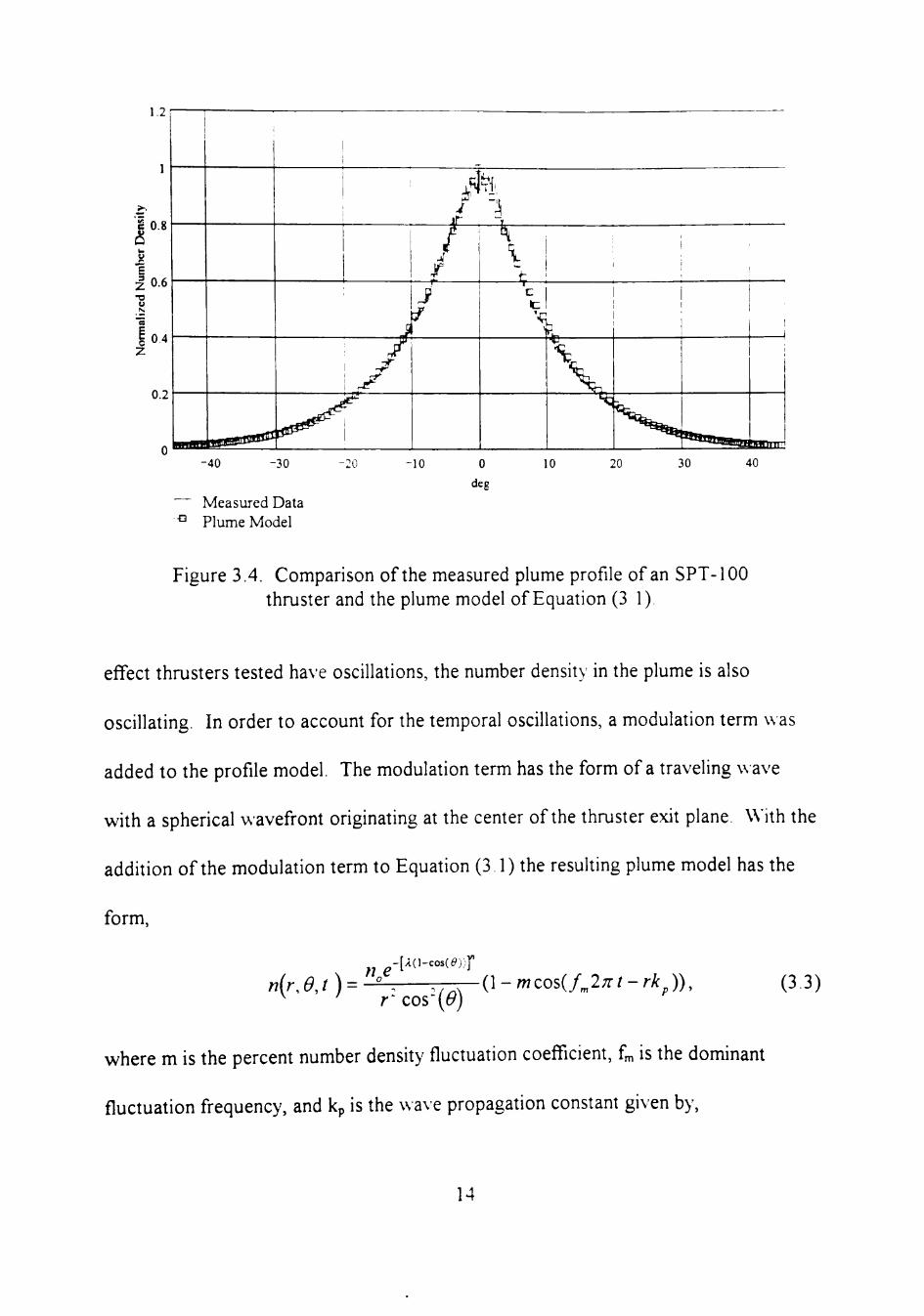
Figure 3.4 gives a comparison between the plume model of Equation (3 1) and the
SPT-100 thruster. In both plots, the fit ofthe model to the measured profile is ver>-
tight and within experimental uncertainty In each ofthe following graphs, the ion
Table 3.1. Plume model coefficients.
Thruster Model D-55
SPT-100
T-lOO
n 0.65
0.65
0.68
X 35
33
37
q 0,3
N/A
N/A
k 1000
N/A
N/A
12

1,2
I" U
B 0,6
o N
o 2
0.4
0.2
1
J^
,' ^ n
\
\
-40 -30 -20 -10 0
deg
10 20 30 40
Measured Data ••° Plume Model
Figure 3.3. Comparison ofthe measured plume profile of a D-55 thruster and the plume model of Equation (3.2),
density distribution was given. An important assumption that was made during the
development of this far field plume model was that the electron and ion number
densities are approximately equal. Although this assumption is reasonable in the far
field, in the confined space of a vacuum tank significant differences between the two
number densities can be present due to charge exchange whh the walls. In addhion,
the near field electron and ion number densities can be different due to the magnetic
field leakage from the thruster. The resuh ofthe magnetic leakage field is a local
increase in the number density around the thruster body.
Accounting for the temporal dependence ofthe plasma plume was the next
step in refining the plume model. Because the discharge currents of all the Hall
13
1.2
I OS
I 0.6 u
04
0.2
HHffnl a««assfl9B5^
1 _
j r «
n^
^ ,
J /
- . 1 ' :
c 1 1 t ! 1 1
\ \
V ^ ^ ^ L
-40 -30
Measured Data ^ Plume Model
-20 -10 0
deg
10 20 30 40
Figure 3.4. Comparison ofthe measured plume profile of an SPT-100 thruster and the plume model of Equation (3 1).
effect thrusters tested have oscillations, the number density in the plume is also
oscillating. In order to account for the temporal oscillations, a modulation term was
added to the profile model. The modulation term has the form of a traveling wave
with a spherical wavefront originating at the center ofthe thruster exit plane. With the
addition ofthe modulation term to Equation (3 1) the resulting plume model has the
form,
-[A(l-cos(^))f
nir.eA^^-. T7T^(l-'wcos(A2;r/-r/:^)), ^ ' r'cos'(^)
(3,3)
where m is the percent number density fluctuation coefficient, f is the dominant
fluctuation frequency, and kp is the wave propagation constant given by,
14

^ = ^ ^ ^ , (3 4) v
F
where Vp is the plume exit velocity The coefficients m and f were determined using a
high-speed Langmuir probe setup. In this experiment, a spherical Langmuir probe was
placed in the plume centerline ofthe thruster under test The probe bias was swept
using a fijnction generator connected to a bipolar amplifier. The average centerline
number denshy, n^ was obtained by measuring the average saturation current across a
100 ohm bias resistor. The current density modulation coefficient, m, and the
modulation frequency, fm, were obtained by applying a constant dc bias on the probe in
the centerline. The current across the probe bias resistor was recorded using the high
speed data acquisition system. A complete description ofthe Langmuir probe setup is
given by Mankowski [4],
As expected, the centerline number density, n^ was highly dependent on the
Xenon mass flow rate to the anode. The cathode gas flow rate also has a large impact
on the number density Under certain operating conditions, the cathode flow rate
would change the number density by 40 percent or more. Typical values of n,. in this
experiment were in the range of 0.4xl0'^ to 1 5xlO'^ under nominal operating
conditions for all the thrusters tested. These numbers are close to those obtained by
Myers [9]. The number density modulation coefficient, m, was obtained graphically
from the high-speed Langmuir current wa\eforms. Figure 3 5 shows the relative
number density as a ftinction of time on the plume centerline of a T-lOO thruster, and
Figure 3.6 shows the associated relative current waveform From the graphs it can be
15

seen that the number density for the T-lOO has a modulation coefficient, m, between
0 02 and 0.16, depending upon the level of current oscillations. In a similar format.
Figure 3.7 shows the relative number density for an SPT-100 with nominal operating
parameters. Figure 3.8 gives the relative discharge current waveform ofthe SPT-100.
The SPT-100 graph shows a peak number density fluctuation of 0.12. The number
density fluctuation and current variation graphs for the D-55 are shown in Figure 3,9
and Figure 3.10, respectively. Note the differences in the vertical axis scale for these
figures.
100
95 -
J 90 E Z
85 -
80
7"
• I. • • , ! ( -
\ -, •, • '• •
I ^ . I \
I
M,,:,5 • ) ! ^ 1
(
1 •'
0.1 0,2 0,3 0,4 0,5 0,6 time (ms)
0.7 0,8 0.9
Figure 3.5. Percent number density of a T-lOO thruster
100
60
I )
t.[ '' ^ /; :
J, , A . r :
1
I I -[ '
1 ! "
< ' 1
i f V
I L 0,1 0.2 0.3 0.4 0.5 0.6
time (ms)
0.7 0.8 0.9
Figure 3.6. Percent peak current waveform for a T-lOO thruster.
16

100
85 0.1 0.2
_L_ 0.8 0.3 0.4 0.5 0.6 0.7
time (ms)
Figure 3 7. Percent number density of an SPT-100 thruster.
0.9
100
c 3
u c .o
50
f I I
\ I
i l l ! !
' ;• i i i l !:
I ' l ihi iMi^
r i\ !!
M M i I 1 M ; I i I I M I i ,/ I h, I I ! ; 1 I I
I ! i
1 ; ' . .' I
'7 1/ V {! {' l V \ I'' \! ' I i M M M1111 i 1; : i i j !; ;; 1M, I 11 w i I 1M n n i \ M / 1/ w II / '' V. I :,i •' \! \: \l V \! ; V ' '' '• ' \' i ' 1/
± 0.1 0.2 0.3 0.4 0.5 0.6
time (ms)
0.7 0.8 0.9
Figure 3.8. Percent peak current waveform for an SPT-100 thruster.
0.1 0.2 0.3 0.4 0.5 0.6
time (ms)
0.7 0,8 0.9
Figure 3.9. Percent number density of a D-55 thruster.
17

100
•S 90
3 O
80
( '
f i l l i f "
M i l I'
70
V\
±
i i I' , f ) .
, i ^ ' ^ ' i l l i l l i . ' ( V ' V '•" 1 1 h I I ' i ' i ' I'l
Vi;;,i I 1 I ) I I I M l I n " • ' t ^
0.1 0.2 0.3 0.7 0,8 0.9 0,4 0,5 0,6 time (ms)
Figure 3.10. Percent peak current waveform for aD-55 thruster.
The D-55 graph shows a number density fluctuation of 3 %. The Langmuir
probe data presented in the previous graphs are representative data only. The
modulation coefficient for each thruster is dependent upon the exact operating
parameters, discharge fiher, and thruster age. Addhional Langmuir probe and current
waveform pairs are presented in Appendix A. The number density modulation factor,
m, can be approximately related to the discharge current fluctuation by a current
sensitivity factor, Csens, given by.
C.„„. = m C
(3.5) mod%
where Cniod% is given by,
C C = 1 - — (3,6)
where C^n and Cmax are the minimum and maximum currents in a given time window.
Values of Cn,odo.. for the three thrusters are in the range of 20 % to 25 %, whh a value
18

of 22.5 % typical for the SPT-100 and T-lOO thrusters and 25 ° o typical for the D- >
thruster.
The primary modulation frequency, f , for the three thrusters was obtained
both graphically and by using an FFT algorithm Although the primary modulation
frequencies ofthe SPT-100 and T-lOO are clearly defined, the number density
waveform ofthe D-55 appears to have no distinguishable primary frequency. As seen
in Figure 3.11, the FFT ofthe D-55 number density waveform is broadband and has
several peaks in the 10 to 70 kHz range. In contrast, the FFT ofthe T-lOO waveform,
shown in Figure 3 12. has a distinct frequency spike at 22 kHz Likewise, the
SPT-100 has a distinct number density oscillation of 27 kHz, .AJthough the
modulation frequency is not as dependent upon the operating parameters as the
modulation index is, small variations in the modulation frequency are observable \\ ith
changes in the magnetic field for each thruster
I 08 C
c.0.6
•V 0.4
E z
02
i! '
1 ' I
I!:: ''Mi '' I
I i\ I J
i l 1 1 I
|!i
I ii ' , . 1 ' M
f I! " ' I I.**! 1 I •!Ui ! I , ' J '
i / l ^ ' I i i U i|i
20 40 60 80 100
kHz
i:c 140 160 180 200
Figure 3.11. FFT ofthe D-55 number denshy waxeform
19

•= 0,8
^0.6 v.
0,4
Z 0,2 I }K
I ,. < I I
20 40 60 80 100 120 140 160 180 20C
kHz
Figure 3 12. FFT of the T-100 number denshy waveform.
The one remaining parameter not determined is the exh velocity. Because the
exit velocity is not easily measured directly, an inference had to be made that the exit
velochy of all three thrusters was similar The reasoning behind this is the fact that the
three thrusters have similar specific impulses and efficiencies, both of which are
directly related to the exit velocity. Whh this assumption, the exit velocity data
obtained by Manzella [10] for the SPT-100 can be applied to the other two thrusters.
The reported exh velocity ofthe SPT-100 is 15 km/s Although an exact exh velocity
for the D-55 and T-lOO has not been determined, the overall effect of this
approximation is negligible when viewed from a communication impact point of view.
With the spatial and temporal coefficients determined for each ofthe three
thrusters, a complete far-field plume model can be assembled A visual representation
of Equation (3.1) using coefficients determined for the SPT-100 is shown in Figure
3 13 Figure 3.14 is a visual representation of the complete plume model described by
20

Equation (3.3) for the SPT-100. Although many ofthe plume model coefficients are
dependent upon the thruster operating parameters, the number density modulation
factor, m, shows the greatest dependence on variations in the thruster operating
parameters.
nt
Figure 3.13. Plot ofthe static plume model for an SPT-100 (5 m square)
nt
Figure 3.14. Plot ofthe complete plume model for an SPT-100 (5 m square).
21

CHAPTER 4
MICROWAVE INTERFEROMETER
A microwave interferometer is a device that is used to obtain the line
integrated number density of a plasma by measuring the phase shift that a microwave
signal experiences when passing through the plasma. Due to the dispersion properties
of a plasma on RF signals, as discussed in Chapter 2, a microwave signal passing
through a plasma undergoes a phase shift relative to a signal propagating in free space.
If the phase shift can be determined and the integration path is known, the line-
integrated number denshy can be extracted using Equation (2 4), In this research, a
microwave interferometer was used for two purposes. The first was to verify the
plume model developed in Chapter 3 and the second was to measure phase transients
of a microwave communication signal propagating through the plume of a Hall effect
plasma thruster.
A schematic diagram of a microwave interferometer is shown in Figure 4,1
The basic system consists of a microwave oscillator, directional coupler, mechanical
phase shifter, and a DC coupled mixer. In the basic microwave interferometer, the
output of a microwave oscillator is fed into a directional coupler, where a portion of
the energy is splh off from the main output. The main output ofthe coupler is passed
on to a horn antenna and is propagated across the plasma volume where h is received
by another horn antenna. The output ofthe receiving antenna is then input into the RF
port of a mixer. The microwave signal split off by the directional coupler is
22

Mecnan.ca Phase Adjuster"
Decoupled . Horn Antenna
Mixer ^ , ^ / /
1 • ^ V
Thruster Plume
>
Horn Antenna
Directional Coupler
-—.
Isolator ^/r~\^\
Microwave Oscillator
. A . Output
Figure 4.1. Schematic diagram of a basic microwave interferometer.
passed through a mechanical phase shifter and into the LO port ofthe mixer. Because
the mixer is DC coupled the IF port will contain a vohage proportional to the sine of
the phase difference between the RF and LO ports. Thus, from the output ofthe
interferometer setup, the phase difference between the signal propagating around the
plasma and the one going through the plasma can be obtained [11].
Although the basic microwave interferometer is adequate for some diagnostics,
it has many problems and limitations when compared to the measurement requirements
of this project. In particular, the far field plasma volume ofthe Hall thrusters on which
the diagnostics are to be performed is large compared to a typical laboratory plasma
where microwave interferometry has tradhionally been used. Because ofthe large
volume, the distance across which the interferometer will be used are large, thus
causing large signal losses in the reference leg of a conventional interferometer,
particularly at higher operating frequencies ( > 10 GHz ). In an effort to overcome the
23

signal loss problem, a microwave interferometer was developed v\ hich uses a low
frequency oscillator as the reference source
The phase sampling microwave interferometer, shown in Figure 4 2. uses a
100 MHz crystal oscillator as a reference source, thus reducing the power loss along
the reference leg ofthe interferometer. In this system, a 6 GHz multiplied cavity
oscillator was phase locked to the reference source using a sampling phase detector
The loop fiher was adjusted to provide a 3 dB bandwidth of 500 kHz. The loop gain
was set sufficiently low to allow a minimum DC phase error of 30 degrees relative to
the reference source. By allowing the large DC phase error, an external control
voltage was added to the automatic frequency control (AFC) vohage, thus providing
an inexpensive electronic phase adjustment in the system. The output ofthe phase
locked oscillator was then transmitted through the plume of a Hall thruster using two
horn antennas. The received signal was input into another sampling phase detector
where its phase was compared to that ofthe 100 MHz reference source. The
SRD Pulse Generator
Mechanical Phase Adjuster
Thruster Plume
Horn Antenna Horn Antenna
100 MHz Xtal. Osc
BRD Pulse Generator
X
6 GHz Multiplied Cavity Osc, w/AFC
^
^ \
Phase Detector Output •Electronic Phase Adjustment
Figure 4.2 Block diagram of a sampling microwave interferometer.
24

output ofthe receiving sampling phase detector was then fihered for aliasing and
amplified and buffered to increase the signal-to-noise ratio at the measurement site
The buffered output ofthe interferometer was connected to a high-speed
analog to dighal (A-to-D) computer board in a 486 computer. The phase data were
collected using a commercial software package that was programmed to provide a
customized interface for this system. Because the maximum sampling frequency ofthe
A to D board was 20 MHz, the system bandwidth was limhed to the 10 MHz Nyquist
frequency. Although the data acquisition system bandwidth is an order of magnitude
lower than that ofthe sampling interferometer, the expected phase shift frequencies are
in the range of DC to 150 kHz and, therefore, the data acquisition system bandwidth
does not significantly limit the performance ofthe overall system.
The primary limitation ofthe system was the high quantization error associated
with using an eight bh A-to-D converter in the data acquishion system Because the
interferometer can uniquely distinguish any phase difference between -90 and +90
degrees, the output ofthe data acquishion system was limited to steps of 0,7 degrees.
In order to overcome this problem, the output amplifier ofthe interferometer was
made adjustable to provide a means of controlling the ftill-scale output vohage. Three
gain levels were chosen to provide fijll scale readings of + - 90 degrees, + - 45
degrees, and + - 25 degrees. These fijll-scale readings correspond to phase
quantizations of 0.7, 0.35, and 0.098 degrees, respectively The background noise
level ofthe interferometer output is highly dependent upon the stability ofthe horn
25

antenna mounts and RF cable vibrations Typical levels of noise were in the range of
0.1 degrees to 0,5 degrees.
The system was calibrated m-situ using a mechanical phase adjuster in the
reference leg. The reference phase was adjusted through a length equal to 360 degrees
at 6 GHz, while the output ofthe interferometer was recorded From the recorded
output, the peak deviations, both positive and negative, were determined, and were
used as coefficients in a fijnction used to convert the output ofthe interferometer to
degrees. Because the output ofthe interferometer is proportional to the sine ofthe
phase difference, the output must be transformed using an inverse sine fijnction ofthe
form.
Phase{l\^,^^ = sin V
ir.l (41)
where \',nt is the interferometer output voltage, V.nnax is the maximum interferometer
output voltage (corresponds to a 90 degree phase difference), ^ ntInln is the minimum
output voltage (corresponds to a -90 degree phase difference), and Phase(\',ni) is the
phase difference in degrees.
26

CR'\PTER 5
PHASE SHIFT MEASLTIEMENTS
The microwave interferometer was used to verify the accurac\ ofthe plume
model developed in Chapter 3. In order to accomplish this, phase shift measurements
were made at several transmission angles and distances relative to the thruster plume
The measured phase shifts were then compared to the theoretical values obtained with
the plume model. During these sets of experiments, the interferometer was nulled
whhout the thruster running. The acquisition system recorded the output voltage at a
sampling frequency of 250 Hz for 32 s. The thruster was started approximately 5 s
after the data acquisition was inhiated. The acquired waveform was then transformed
using Equation (3.3) The resulting waveform gives the phase difference between a
microwave signal propagating with and without the thruster plasma plume present
The first set of tests was conducted on axis with the signal propagation path
parallel to the thruster exh plane. The distance from the exit plane was 0,5 m, A
sketch ofthe test setup is shown in Figure 5 1, Due to time constraints in the vacuum
tank facilities at NASA Lewis Research Center, the T-lOO was the only thruster tested
at this distance. Figure 5.2 shows the measured phase shift of a 6 2 GHz signal during
the startup of a T-100. The T-lOO exhibits a large over-shoot before stabilizing to a
value of 45 deg. The overshoot is probably due to ionization ofthe Xenon atoms
diffijsing out the end ofthe thruster before ignition. After ignhion,
27

/ > « '.'"..'..'...
2,0 m
Figure 5.1. Sketch of parallel propagation path (relative to the exit plane).
100
80
60
00
40
20
0 -1
1
IL p. 1 V
t|i>.'VWffA«JMV^ '^H^VV^fl^Jy ' ' • ^ i i i L
^ ^ ^**^*Asy,r>y,>*A
l iJV^
AitJT
1.8 2.686 3.571 6.229 7.114 4.457 5.343
time (s)
Figure 5.2. Parallel start-up phase shift at 0.5 m for a T-100.
28

the accelerated ions collide with the neutral atoms, causing the atoms to ionize and
undergo a momentum change in the direction ofthe exhaust plume Using the
Mathcad worksheet contained in Appendix B, the line-integrated phase shift of
Equation (2.3) was calculated using the number density profile described by
Equation (3.1). A phase shift of 45 deg corresponds to a 1 m centerline number
density, no of 0.6 x 10 ^ m'^
A similar start-up plot for the SPT-100 is shown in Figure 5 3. In this plot the
start-up phase shift is approximately 27 deg. The propagation path geometry' is similar
to that in Figure 5.1 except that the distance down from the thruster exit was changed
to 0.9 m because a different vacuum tank was used. Usine the same Mathcad
worksheet for perpendicular propagation paths, a 25 deg phase shift gives a
corresponding value of no of 0.62 x 10 ^ m" . The start-up plot for a D-55 is given in
Figure 5.4. The propagation path was identical to that ofthe SPT-100 test In this
plot, the phase shift is approximately 27 deg at 6.2 GHz. The corresponding value of
no at this distance and propagation path is 0.65 x lO' m ' The D-55 and SPT-100 did
not exhibh the same number density overshoot, during startup, at 0 9 m as did the T-
100 at 0.5m.
The next set of start-up tests used the propagation path shown in Figure 5.5.
The path crossed through the plume plasma on axis at a 45 deg angle and was received
1 m down stream from the thruster exit plane. The main limitation with this
configuration was the finite tank size which caused some ofthe plume to deflect back
29

into the propagation path With the additional particles along the propagation path,
the measured phase shift should be greater than that predicted by the model
40
30
^ 20
I'M* I t)i/i .r'
wm'^i A
in ^ H I
' , 1 II' M M H' l ji ^ ^ ^ ^
3.714 6.5"1 286 4 429 5 143 5.857
time (s)
Figure 5.3. Perpendicular start-up phase shift at 0.9 m for an SPT-100.
30
20
M 10
-10
" • . ^ . — ^
^.^- -J-f.J.'^'^'' v-.- _- V
2.429 2.857 3.286 3."14
time (s)
4.143 4.571
Figure 5.4. Perpendicular start-up phase shift at 0.9 m for a D-55
30

Figure 5.6 shows the startup phase shift for the D-55. The measured phase
shift shown in the figure is approximately 50 deg. Appendix B contains a Mathcad
worksheet developed to calculate the phase shift along diagonal propagation paths.
Using this worksheet, a predicted phase shift of 50 deg for this thruster corresponds to
a 1 m centerline number density, rio, of 0.66 x 10 m . Although the increase of no
J6 „ -3 (from 0.65 x 10 m " to 0.66 x 10 m ) between the perpendicular and diagonal
propagation paths is not beyond experimental error, the number does indicate that the
finite tank size can be causing an artificial increase in the plume number density along
the propagation path. The startup phase shift waveform for the SPT-100 along the
same propagation path is shown in Figure 5.7. The SPT-100 shows a phase shift
Figure 5.5. Sketch of 45 deg propagation path.
31

bU
50
40
^ 30
20
10
0
1
i
i 1
' • _ * / - ^ — ^ •
6.286 6,571 7.429 7.714 6.857 7.143 time (s)
Figure 5.6. Startup phase shift along a 45 deg propagation path for a D-55
8
of approximately 52 deg along the diagonal propagation path. A centerline number
density of 0 68 x lO' m" corresponds to this phase shift. As whh the D-55 diagonal
propagation path startup waveforms, the SPT-100 shows a slight increase in no due to
the fimte tank size.
The next set of startup traces was taken whh a propagation path on axis 0.5 m
to the side and perpendicular to the exh plane of a D-55. The receiving horn was
placed 2 m from the exh plane, and as was the case for the diagonal propagation path,
the finite tank size can cause an artificial increase in the number density along the
propagation path. Because the tank diameter is approximately 2 5 m, and the D-55
thruster has a significant ion flux at 45 deg, deflected ions will cross back into the
propagation path at a distanced of 1 m and greater away from the exit plane. The
phase shift for the D-55 perpendicular startup shown in Figure 5.8 is approximately
32

60
40
20
0 •*"~ • ~ 2,5
I ' . L 1 h ^ ' ' ;
,i. ^^^^AVV' '."'''V // rvvr '' - ' > •,W'^'>V
3,5 5,5 4 4,5 5 time (s)
Figure 5 7. Startup phase shift along a 45 deg propagation path for an SPT-100.
25
20
15
r
1
i
1
i
. J
f 1
1
i t * ; " " ' '
r
'.••.T-'^-'-^j,""rAi»u*->, . . . . '-> . -
0.5 1.571 2,643 3,714 4.786
time (s)
5,857 6,929
Figure 5.8. Startup phase shift along a propagation path perpendicular to the exh plane of a D-55
33

22 deg. Changing the propagation angle to 0 deg and the exit distance to 2 m in the
diagonal Mathcad worksheet, resuhs in a value of 1 x lO' m' for no. The predicted
phase shift along this propagation path with no equal to 0.6 x lO'Ss 15 deg.
The final startup test was conducted on an "end-of-life ' SPT-100 thruster in a
large tank facility at NASA Lewis, Unlike the previous tests, this test was conducted
in conjunction with a plume deposhion experiment and therefore cylindrical
collimators were placed along a semi-circle in the thruster's exhaust plume. Due to
limitations on time and on the number of suitable mounting points in the tank, the
transmitting and receiving horn antennas were positioned such that the propagation
path was in the same plane as the collimators. In particular, the propagation path was
on axis and started 1.8 m to the side ofthe thruster and traveled at a 31 deg angle
relative to the exit plane, whh the receiving antenna 6 m from the exit plane. Because
the collimators partially blocked the accelerated ions along the propagation path, the
phase shift measured was expected to be smaller than predicted by the plume model.
Figure 5,9 shows the startup phase shift for the end-of-life SPT-100 The
oscillatory startup was caused by an incorrectly set current limit and is not a normal
phenomena. The measured phase shift is approximately 9,5 deg This corresponds to
an no of 0.5 x 10 ^ m' to achieve the same phase shift according to the plume model.
Although the lower phase shift is probably due to the collimators, inaccuracies in the
antenna placements and the fact that the thruster was tested at the end-of-life could
also account for the difference. Overall however, the predicted phase shift is within 15
percent ofthe model prediction,
34

12
10
^. 6 i ln./i i l ' l '
(f'14
+t TTTTT l\Ul'
M,
, ! !•
^.^'f-
T T
-H-
' .lililllhj M - ' : I
P i l i ^
il ' II II !i II
I t 1
, . (r
28,85" 35.'14 42 5"1 49 429 56.286 63 143 70
time (s)
Figure 5.9 Startup phase shift along a diagonal propagation path for an end-of-life SPT-100,
The last ofthe low speed (i,e,, several seconds) phase shift measurements were
made on the D-55 thruster. During these tests, the cathode flow rate was changed
from 0,2 mg/s to 1.6 ma s while the thruster was running. The interferometer was
zeroed whh the thruster running at the lower cathode flow rate The propagation path
was the same diagonal path described previously for the D-55 tests. In Figure 5.10 the
phase shift changes 29 deg between the minimum cathode flow rate and the maximum
flow rate. Based upon the previous resuhs and addhional tests conducted away from
the designed operating point ofthe thruster, the value of no was determined to have a
dependence on the cathode flow rate greater than ± 20 percent ofthe nominal value
Although significant charge exchange with the tank walls will occur at the two cathode
flow rate extremes, this does indicate the influence ofthe cathode on the thruster
plume denshy
35

30
20
Ob
10
0
/
\ 1
/
i
> •
^V^-jr^.-nri — , — 1 r — - - • — ^ - * — - L ^ - Y . • •4^.^.^^>-^
0 5.714 11.429 17.143 22 857 28.571 34.286
time (s)
Figure 5,10, Change in phase shift due to change in cathode flow rate for a D-55 (0,2mg/s at 2 sec linearly to 1.6 mg/s at 28 sec).
40
The next set of experiments was designed to provide information on the
frequency and magnitude of phase fluctuations that a microwave communication signal
would experience propagating through the plume of a Hall effect thruster. During
these tests, the microwave interferometer was adjusted to provide an average phase
shift of zero while the Hall thruster was operating under steady-state conditions The
output ofthe interferometer was sampled and recorded at a rate of 10' samples per
second, resuhing in a maximum detectable frequency of 5 MHz, The recorded output
was then transformed using Equation (4,1) and plotted to illustrate graphically the
transient phase shifts. In addhion, the current waveform was also acquired and is
plotted for comparison whh each phase shift plot. Because these tests were conducted
in conjunction with the start-up tests discussed previously, the previous section should
36

be referred to for a complete description ofthe propagation path, as only a brief
description ofthe path will be given in this section.
Figure 5.11 shows the measured phase shift transients caused by a T-100
plasma plume with the parallel propagation path discussed previously. Figure 5.12 is
the associated current waveform taken at the same time Figure 5.11 indicates that the
T-100 is causing phase transients in excess of 20 deg peak to peak, A comparison of
Figure 5.11 and 5.12 shows a distinct correlation between the amplitude and frequency
ofthe current oscillations to those in the phase shift plot In a previous section, it was
shown that the T-100 exhibited a current sensitivhy factor Csem of 0,225, which relates
the current oscillations to the number denshy modulation factor, m In a time window
from 3.1 ms to 3.3 ms, Cmod% is found to be 0.5 which resuhs in a modulation factor,
m, of 11 percent. As a comparison, the predicted phase oscillation using the temporal
plume model are shown in Figure 5,13, The plot shows the predicted
20
4 0
-10
-20
, ' • I 1 . ' il 1
', '-^ >f. • 1' , t I '
II
f
f
{
1,
t " * r ' 1
. . 1 - ' ' i
li 1
i
V
t
1
U 1 '
1 ' 1
1 ,
> . 1
"• 1
, ' 1
t>
( ' ' , ' ' .' •'
1 1 1
1 ''' ^ • • , 1 - ,
1 >
r ( 1 i: (1 "
• . ' , ' • -
' - 1 V
1 '
' P./ -»
1 1
1 ' /I
' " A 1 .. ' W
!• ' '
j '
1
1
i\
11 1
* t>
2,5 3,5 time (ms)
4.5
Figure 5.11. Measured phase transients of a 6 GHz signal propagating along a parallel path (relative to the exit plane) through the plume of a T-100.
37

10
l i l
I I I ! , , , . , . , , | l i | , ,
1
1
' 1 rl: > 1 1 . i 1
•1
1
I , , h ' .
• ,1
' i ' I ' r , '
1 . 1 ' I
'hi' 1 ' ' '
J I
.11-1. A I ' V - '
Ml 1
2,5 35
time (ms)
4,5
Figure 5.12. Current waveform for the T-100 in Figure 5 11
60
55
50 . , r ! i\ I 1
' I I ,
iL 45
40
35
A A ;. /' A ' A l\ : > M ' I 1
TTTT iIlM/ Il !i I i I i M i
V V ^ . i!
30 1 25 5 10 15 20
modulation factor m (%)
Figure 5.13. Predicted phase shift along a parallel propagation path 0.5 m down from the exh plane as a fijnction of m, for the T-100
3u
phase oscillation as the modulation factor m is varied from 0 percent to 30 percent
From the graph h is found that a value of 11 percent for m results in a predicted phase
shift of 9 deg. This value is almost identical to the measured value in the same time
window. Likewise, other time windows can be examined with similar results.
Because the current oscillations ofthe T-100 are not constant, a direct comparison
cannot be made, however, the predicted phase shift is whhin a reasonable error ofthe
38

measured phase shift, given the instability ofthe thruster and the complexity ofthe
problem.
The phase transient data and associated current waveform for the SPT-100
along the parallel propagation path are shown in Figure 5 14 and Figure 5,15,
respectively Because the SPT-100 thruster was configured to operated with the
current to the electromagnets in series with discharge voltage, no magnetic field
augmentation was possible As a result, the current oscillations during this test were
considered excessive and not a true representation ofthe potential stability ofthe SPT-
100 thruster Subsequent results, presented below, will show that the SPT-100 is
highly dependent upon the discharge power supply design and filter In addition, the
use of a separate power supply for magnetic field augmentation has been shown to
reduce the amplitude ofthe current oscillations [3] To compare the accuracy ofthe
plume model and the current sensitivity factor, Csens, the predicted phase shift along the
given path for values of m ranging from 0 to 0,3 is shown in Figure 5 16, From Figure
5.15 the value of Cn,od% is determined to be 0.9, resuhing in a predicted modulation
factor, m, of 21 percent. A predicted phase shift of 9 deg corresponds to a 21 percent
modulation factor using Figure 5.16, This resuhs in an overall phase shift prediction
error of 10 percent given only the current waveform
During the 45 deg diagonal propagation path testing ofthe SPT-100, the
magnetic field coils were connected to a separate power supply, thus allowing the
magnetic field to be augmented. The separate supply allowed the thruster to be
adjusted to provide a more stable current waveform. Figure 5 17 shows the phase
39

10
^ 0
-5
-10
I—TT nn—rr •^TT
rtm i i i ' * ' '
M-1 1 I I
0.5
1 I
J L - T T - ^
TT
r
• 1 , I
I , > I . I TT -U-
2.5 1 1,5 2
time (ms)
Figure 5,14. Measured phase transients of a 6 GHz signal propagating along a parallel propagation path through the plume of an SPT-100,
10
8 • '
1
i l , 1
• • ' • ! ; i / '
j 1 1 ' 1 , ' t > . 1 . '
Ii 1 1 M
,! i l '
' ' ; ' • : ' "
, 1 • > 1 ^ ' V V » . . ' ,
i l ! I | (
i
. ' ' ' . > 1 • i » . , 1
. 1 , i . • 1
1
i '• i ' i I
,
1 • » 1 . 1 1 , 1 " ' ' * '
1 t
(
, !
1! 1
1 11
1 ! !
'' 1
^1
' 1 1. I • ! 1 1 . ! 1
0.5 1.5 1 ^
time (ms)
Figure 5 15 Current waveform for the SPT-100 in Figure 5 14
35
30
^ 25
20
15
-^"^ JL A
^' V V f^ f\ A A A '\ l\ \ i\
i I
mnn V I' I . 1 • M M ! l i 1 y i' ! n I 1
V I
1 10 15 20
modulation factor m ("o) 25 30
Figure 5 16, Predicted phase transients of a 6 GHz signal along a parallel propagation path 0,9 m down from the exh plane as a function of m
40
transient waveform recorded during this test with the associated current waveform in
Figure 5.18. Examining the current waveform in a time window from 0.8 ms to 0.9
ms gives a value of 0.375 for Cn,od%, resuhing in a predicted modulation factor, m, of 8
percent. Figure 5.19 shows a predicted phase transient of 5 deg for this value of m
along the described propagation path. In Figure 5 17, the measured phase shift during
this time window is approximately 5 deg, thus showing that the phase shift prediction
by the model is accurate.
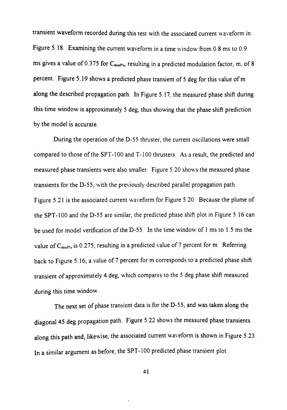
During the operation ofthe D-55 thruster, the current oscillations were small
compared to those ofthe SPT-100 and T-100 thrusters. As a result, the predicted and
measured phase transients were also smaller. Figure 5.20 shows the measured phase
transients for the D-55, whh the previously described parallel propagation path.
Figure 5.21 is the associated current waveform for Figure 5.20. Because the plume of
the SPT-100 and the D-55 are similar, the predicted phase shift plot in Figure 5.16 can
be used for model verification ofthe D-55. In the time window of 1 ms to 1.5 ms the
value of Cmod% is 0.275, resulting in a predicted value of 7 percent for m Referring
back to Figure 5.16, a value of 7 percent for m corresponds to a predicted phase shift
transient of approximately 4 deg, which compares to the 5 deg phase shift measured
during this time window.
The next set of phase transient data is for the D-55, and was taken along the
diagonal 45 deg propagation path. Figure 5.22 shows the measured phase transients
along this path and, likewise, the associated current waveform is shown in Figure 5.23
In a similar argument as before, the SPT-100 predicted phase transient plot
41

•^ 0
, , . ^ . .
• • . P l ^
'I ih.
— i -
!...., 1: •/ (
11( I
1 . 1 I r
\'::vj —TH
iM
' • • ' • ' • ' ' - h j r : ' ^•'iijli^
I . < l i
. ' . . > - ' •
' • . , :
0,5 •> « 1 15 : time (ms)
Figure 5.17 Measured phase transients of a 6 GHz signal propagating along a 45 deg diagonal propagation path for an SPT-100
10
8
, 1 ' l . l .
r. ' I
, , - : ' - | ' > '
• ! , i ' <
1
\
t 1 r . . 1
1 1 1
( • '
i 1
Ij'l
• • 1
' 1 1 ( ' - 1
\
' 1
!
1
• '}•:
iM ' l i , ,
- • • • • • i , • • , • ^ • •
1 0 417 0 833 1 t6' 083 1 25
time (ms)
Figure 5 18 Current waveform for the SPT-100 in Fiaure " P
6C
55
.2 50
45
40
' ^ . - / u W i l l i l l i i ' n
I ! > I
^^v i ' i ' v . .V i i j |H jy j | j j i
10 15 20 modulation factor rr, ('o)
3:
Fieure 5,19. Predicted phase transients along 45 deg diagonal propagation path at 1 m down from the exh plane as a fijnction of m
42

for the 45 deg diagonal propagation path will be used for comparison to the model In
a time window from 0.4 ms to 0.7 ms, the value of C od is 0 2, which gives a
predicted modulation factor, m, of 5 percent. Figure 5.19 gives a predicted phase shift
transient value of 3 deg for this value of m. A comparison ofthe 3 deg prediction and
the measured 1.5 deg shows a 50 percent error Although this is a large percentage
error, the difference error is small compared to the static phase shift that the transients
are added to.
The final phase transient data were taken on the end-of-life SPT-100 in the
large vacuum tank facility. The propagation path was the 31 deg diagonal path
described previously. During this test, an integrated power processing unit, that
contained all the necessary power supplies and mass flow controllers, was used to
operate the thruster. The power processing unh was designed and optimized
specifically for the SPT-100 and is the same type that will be used on fijture space
missions involving the SPT-100. Figure 5.24 shows the measured phase transient
waveform recorded during this test. The associated current waveform is shown in
Figure 5.25. A significant decrease in the amplitude ofthe current oscillations over
previous tests involving the SPT-100 is apparent. As a result, the measured phase
transients are expected to be smaller in amplitude as well. Figure 5.26 shows the
predicted phase transients along the propagation path for values of m from 0 to 0.3.
From Figure 5.25 a value of Cmod% can be calculated to be 0 275 in the time window
from 0 to 1.5 ms. This corresponds to a predicted modulation factor, m, of 6.1
percent. In Figure 5.26, an m factor of 6,1 percent corresponds to a predicted phase
43

.^ 0
-2
:iiiuMiML m Ti ijjjhift .jiLllJ-MJMilul r iM
0.5 15 time (ms)
Figure 5.20. Measured phase transients of a 6 GHz signal propagating along the parallel propagation path through the plume of a D-55
10
'•'f i''>t'^^^''"•^'' ;'.^'jj4iv,.ic>->^ ;,F,.v„-.>'..' - ,'vAi' ^^[ ihSlTi i rv; '
0.5 1 15 :
time ims)
Figure 5,21, Current waveform for the D-55 in Figure 5 20
= 1
fJl E Ul iiUI i ! I l
JLOI n 0.1 0.2 0,3 0.4
time ims i
0.6
Figure 5,22 Measured phase transients of a 6 GHz signal propagating along a 45 deg diagonal propagation path for a D-55
44

10
» , - w
T !iL-i:^ W-.' ' iU'\ . j '4. '--- ' .
— • • ? ' ' « • i I i l-W' / ' -' ' '*, ' l I I " ' . * - • 1 •-. 'J :i=X
, li J ^ , •< ^ - «
0.1 0.2 0,5 06 0,3 0 4 time (ms)
Figure 5,23 Current waveform for Figure 5,22,
0,7
w iMl ^!'i'
m .f'V •4
fall \
',T"V ^11', i.i ?
fe^ ''t;V ' :f
-1
time (ms)
Figure 5.24. Measured phase transients of a 6 GHz signal propagating along a 31 deg propagation path for an end-of-life SPT-100.
10
^il11|l|#' \m^ Miii\ii\W imM^kMmfW^ 1^ j t 4yL,.
1 2 3 4 5 6 tmie (ms)
Figure 5.25. Current waveform for Figure 5 24.
45

114
11.3
ac
11.2
11.1 10 15 20
modulation factor m (%)
25 30
Figure 5.26, Predicted phase transients along 31 deg diagonal propagation path at 1.8 m to the side of an SPT-100 as a fijnction ofm
shift of 0.08 deg. In comparison, the measured phase transients during the same time
interval are greater than 0,2 deg, which corresponds to an error in excess of 40
percent. Again, due to the small phase transients being investigated along this
propagation path, the difference in the two values is small enough to make engineering
decisions about the potential impacts ofthe thruster based upon the developed plume
model.
Further examination of Figure 5 24 shows that an unexplainaed phase jump in
excess of 1,5 deg occurs at 1.75 ms, which correlates to a small current drop at
approximately 1 7 ms. The small current drop is probabK due to the closing and
opening of a thermal valve used in the regulation ofthe mass flow to the anode. The
phase transient that followed the current drop is much larger than can be explained by
the model, and may be a random occurrence caused by system noise or most likely by
factors not considered in the model, such as material randomly flaking from the
discharge chamber, perturbing the thruster's plume. Previous studies on the SPT-100
46

have shown that random periodic flaking of deposited material on the discharge
insulator occurs after several hundred hours of testing [12, 13] The researchers
conducting these studies have theorized that the material is due to the vacuum tank
facilities and will not be present in the space environment In any event, this
phenomenon may require fijrther investigation to build a more accurate description of
the potential communications impact of this thruster.
47

CHAPTER 6
PHASE NOISE
In Chapter 5, h was shown that the phase of a microwave signal is changed as
it propagates through the plume of a Hall effect thruster. Although the phase
fluctuations were found to be oscillatory in many instances, a random or non-
deterministic component was present in all ofthe recorded phase transient
measurements. Due to these random phase fluctuations, the power spectral density of
f(t)r in Equation (2.6) will show broading around the carrier frequency, ©c,
proportional to the amplhude and spectral content ofthe phase fluctuations caused by
the plasma plume. Although an increase in phase noise will impact the performance of
communication systems in different ways, depending upon the application and
modulation scheme, the most notable is the limitation on how close adjacent
communication channels can be spaced in the frequency domain. Because the system
degradation due to phase noise cannot be overcome by addhional transmitter power,
any increase in phase noise due to the transmitting media would be considered a
source of concern for most communication systems. It should be noted that the phase
•noise should not be mistaken for the typical noise figure that is often stated for
communication systems, which can be reduced by increased transmitter power
Typically, the system phase noise is dominated by the phase noise ofthe
transmitter and receiver oscillators. In high quality satellhe communication systems,
the microwave oscillators are designed to provide low phase noise and are usually
state ofthe art. When determining the system phase noise, a communication system
48

integrator will typically use the output phase noise ofthe oscillators and include a
small increase due to the amplifiers, mixers, and other components in the system.
Overall, however, the peripheral components contribute a small fraction to the phase
noise when compared to the phase noise ofthe local oscillator Historicalh', the phase
noise increase due to the transmission media was limited to random atmospheric
disturbances such as lightning strikes and is therefore not typically considered a major
contributor to the system phase noise parameter. Because the plume of a Hall effect
thruster has been shown to change the phase of an RF signal propagating through it,
an investigation to determine if the plume significantly increases the phase noise ofthe
RF signal was made
To qualify and quantify the effects ofthe Hall thruster's plume on RF signal
phase noise, a test setup was devised which transmits a microwave signal through the
plume using a low phase noise cavity multiplied oscillator as the transmitting source
A pair of microwave horn antennas were placed across the plume, with the source
oscillator feeding the transmitting antenna and the output ofthe receiving antenna
being sent to a microwave spectrum analyzer, A diagram ofthe test setup is shown in
Figure 6 1 During the operation of this test setup, a baseline ofthe power spectral
density ofthe received signal, propagating along a given path, was obtained without
the thruster running using the spectrum analyzer. The data were downloaded and
stored for future plotting using a laptop computer. After the baseline signal was
obtained, the thruster was started and allowed to stabilize. After stabilization, the
49

Spectrum Analyzer
il D D D D D D D D D
O
, /
' \
Horn Antenna
Thruster Plume
^ . • ? • •
Horn Antenna 5 QHZ r.lultiplied Cavity Osc. Phase
Locked to a 100 MHz Xtol. Osc.
Figure 6.1. Phase noise test setup.
power spectral density ofthe received signal was acquired for comparison to the
basehne spectrum. In each ofthe following spectrum plots, the dashed line is the
baseline signal, and the solid line is the received spectrum with the thruster running.
As with the phase transient measurements, the phase noise measurements were made
in conjunction whh the startup phase measurements and thus the propagation paths
described in Chapter 5 should be referenced, as only a brief description will be given in
this section.
Figure 6.2 shows the received power spectral denshy of a 6 GHz signal passing
through the plume of a T-100 along the parallel propagation path, 0.5 m from the exh
plane. Because the settings ofthe spectrum analyzer, such as the frequency span,
resolution bandwidth, and video bandwidth affect how the spectrum ofthe signal is
displayed, the settings of each plot were adjusted to provide the best representation of
the difference between the baseline signal the signal passing through the plume ofthe
thruster. In addition, each plot is normalized to 0 dBm at its peak. Figure 6.3 shows
the current waveform acquired at the same time as the spectrum plot in Figure 6 2 .\
comparison ofthe baseline spectrum to the spectrum
50

E T3
3
"S.
20
-40
-60
->/v^- ' ^
-80 6183.5 6183.667 6183.833 6184
Frequency (MHz)
6184167 6184333 6184.5
T-100 Running Baseline
Figure 6.2 Spectrum of a received signal with and without a T-100 running (1 MHz span).
Figure 6.3. Current waveform ofthe T-100 in Figure 6.2.
ofthe received signal with the thruster running shows that a significant increase in
the phase noise has occurred. At a carrier offset of 250 kHz the increase is greater
than 45 dBm. Although this is not a propagation path that is likely to occur on a
commercial satellite, it does indicate the potential for communication system
51

degradation. Figure 6.4 shows the spectrum comparisons for the SPT-100 with a
parallel propagation path 0.9 m from the exit plane. Figure 6.5 shows the current
waveform acquired at the same time as the data in Figure 6.4. Note that the primary
frequency ofthe discharge current oscillations is approximately 25 kHz. This
corresponds to the distance from the carrier to the first periodic peak in the spectrum
6182,9 6182,933 6182.967 6183 6183.033 6183.067
Frequency (MHz)
6183.1
SPT-100 Running Baseline
Figure 6.4 Spectrum of a received signal with and without an SPT-100 running (200 kHz span).
Figure 6.5. Current waveform ofthe SPT-100 in Figure 6.4.
52

ofthe received signal. It also is the distance between subsequent peaks in the
received spectrum, which follows the well-known communication theory of phase
modulated signals. In addition to the periodic peaks, a significant increase in the
phase noise across the entire 200 kHz span is present.
The next spectrum plot, shown in Figure 6.6, is for the D-55 with a parallel
propagation path. Figure 6.7 shows the associated current waveform for Figure 6.6.
Because the D-55 is characterized by broad band discharge oscillations, the number
density modulation has no primary frequency. As a result, the spectrum in Figure 6.6
shows broad phase noise with little sideband development. In addition, the level of
phase noise produced is significantly less than that ofthe SPT-100 or T-100. The
lower phase noise is attributed to the magnitude ofthe current oscillations being
much smaller. Because the spectrum analyzer used has a limited dynamic range of
approximately 75 dB at a 200 kHz span, an accurate comparison ofthe phase noise
618-4 966 6184.999
D-55 Running Baseline
6185.033 6185,066 6185099 Frequency (MHz)
6185133 6185,166
Figure 6.6 Spectrum of a received signal with and without a D-55 running (200 kHz span).
53

-;-/-nr;.'', \ ^ , ; / . A, . • 1
;• / .a.-• . ' . • -
• I ' I •
1
1
* •
V •
0.1 0.2 0.3 0.4 ms
0.5 0.6 0.7
Figure 6.7 Current waveform ofthe D-55 in Figure 6.6.
whh and whhout the thruster running is not possible. However, the minimum increase
in the phase noise level is clearly greater than 15 dB,
The spectrum plot for the SPT-100 along the 45 deg diagonal propagation
path is shown in Figure 6,8 with the associated current waveforms shown in
Figure 6,9. In these figures, the data acquired for two operating condhions ofthe
SPT-100 are shown for comparison. When operating whh the clearly unstable
discharge current shown in Figure 6.9 the power spectral density ofthe 6 GHz signal
shows a significant increase in sideband development approximately 30 kHz from the
carrier, corresponding to the primar>' frequency ofthe discharge current oscillation. In
addhion, an overall increase in the phase noise level is also evident. In contrast, the
more stable operating condition shows a significant decrease in the sideband
development as well as an overall decrease in the noise level. Even with the SPT-100
operating with a stable discharge current, the phase noise level is increased by 30 dB
or more along this propagation path.
54

6184.95 6184.967
- SPT-100 Stable — SPT-100 unstable
Baseline
6184.983 6185
Frequency (MHz)
6185.017 6185 03? 6185,05
Figure 6.8 Spectrum of a received signal with and without an SPT-100 running along the 45 deg diagonal propagation path( 100 kHz span).
ms
Figure 6.9. Current waveforms ofthe SPT-100 in Figure 6.8.
The next set of plots show the power spectral density and current waveforms
with a D-55 operating at a discharge current level of 3.5 A and 4.5 A. The
propagation path ofthe 6 GHz signal was the same 45 deg diagonal path used in the
SPT-100 test. Figure 6.10 shows a distinct increase in the phase noise level with the
55

D-55 operating at a discharge current level of 4.5 A compared to 3.5 A. The phase
noise level at 4.5 A is greater than 4 times the phase noise level at 3.5 A. The current
waveforms, shown in Figure 6.11, show no significant increase in the level of current
oscillations between the two current levels.
-80 6184.9 6184.933
D-55 3.5 A D-55 4.5 A Baseline
6184.%7 6185 6185.033 Frequency (MHz)
6185.067 61851
Figure 6.10 Spectrum of a received signal along the 45 deg diagonal propagation path with a D-55 operating at 3.5 A and 4.5 A (200 kHz span).
Figure 6.11. Current waveforms of the D-55 in Figure 6.10.
56

The final phase noise data are for the end-of-life SPT-100 operating in the
large vacuum tank facility at N.^SA Lewis Research Center. The propagation path for
this test was normal to the exh plane and 1.8 m to the side ofthe thruster body The
receiving antenna was 6 m from the exit plane. Figure 6 12 shows the received
spectrum of a 6 GHz signal propagating along the above described path Figure 6.13
shows the current waveform acquired during this test. As with the previous end-of-
life SPT-100 current waveforms, the magnitude ofthe current oscillations are small
compared to newer SPT-100, used in other tests. Although age may be a factor in the
reduced current oscillation level, the refinement ofthe discharge power supply output
filter is the most likely reason for the improvement. As a result, the signal phase noise
level is correspondingly lower In addition, the lower number density along this path
will also contribute to a lower phase noise level. The highest spectral noise level
occurs at approximately 25 kHz from the carrier, which corresponds to the primary
frequency ofthe discharge oscillation.
To verify the effects of transmission frequency, the spectrum of a 2 8 GHz
signal, propagating along the same path was acquired Because the phase shift caused
by a plasma is greater at lower frequencies closer to the plasma frequency, the phase
noise of a 2.8 GHz signal would be expected to increase more than that of a 6 GHz
signal, with all other parameters equal As can be seen, the measured power spectral
density ofthe 2.8 GHz signal, shown in Figure 6.14, has a significant increase in phase
noise over the 6.2 GHz signal. At 2.8 GHz, the end-of-life SPT-100 caused an
increase in the signal phase noise in excess of 40 dB, while at 6 2 GHz the thruster
57

thruster caused less than a 10 dB increase. It should be noted that the power spectral
densities in Figures 6.12 and 6.14 were acquired within minutes of each other, with
the same operating conditions and level of current oscillations.
-80 6212.9 6212.933 6212.967 6213 6213.033
Frequency (MHz)
SPT-100 Running Baseline
6213.067 6213.1
Figure 6.12 Spectrum of a 6 GHz received signal with and without an end-of-life SPT-100 running (200 kHz span).
^AA/V^VVV^U^''' V\ A/VVY-U->'VW /\rV|/^Vvi/VA/v / O A A ^ V ^ Y ^ 4/V\/\/vA^VV-v-'
0.2 0.4 0.6
ms
0.8
Figure 6.13. Current waveform ofthe end-of-life SPT-100 in Figure 6.12.
58

2801.625 2801.75 2801.875 2802 2802.125 Frequency (MHz)
— SPT-100 Running Baseline
2802.25 2802.375
Figure 6.14 Spectrum of a 2.8 GHz received signal with and without an end-of-life SPT-100 running (750 kHz span).
59

CHAPTER 7
CONCLUSIONS
An important engineering model was developed, which allows a satellite
system integrator to predict the impacts of Hall effect thrusters on communication
systems. Although the basic plume model is probably valid for all types of Hall effect
thrusters, plume parameters were determined for three thrusters in particular, the D-
55, SPT-100, and T-100. The plume model developed predicts the stationary electron
number denshy in the plume far field. The model also accounts for the temporal
dependence ofthe electron number denshy caused by the discharge current
instabihties. Langmuir probe measurements, both high speed and swept, were
performed to determine the spatial and temporal parameters ofthe plasma plume
In an effort to verify the plume model and refine it if necessary, a microwave
interferometer was designed and built. The interferometer uses a phase samphng
technique which allows accurate phase shift measurements to be performed across
large plasma volumes. Although the interferometer was designed to be broadband
(1 GHz to 20 GHz), the majority ofthe measurements were made at 6 GHz due to the
availability of low noise sources and the applicability ofthe measurements to the
current 6 GHz satellite communication links. The noise level ofthe interferometer
system was typically less than .05 deg at 6 GHz.
The sampling microwave interferometer was used to perform startup phase
shift measurements on the three thrusters. Using several propagation paths, the phase
60

shift predicted by the plume model was compared to the measured phase shifts along
the same paths. The plume model accuracy during the startup tests was typically
better than 90 percent. The largest source of error was most likely from the effects of
a finite test chamber, causing charge exchange and plume reflux.
In addhion to the startup phase measurements, the interferometer was used in a
high-speed mode to determine the amplitude and frequency of phase oscillations and
transients caused by the plasma plume on a microwave signal. Due to the dependence
ofthe number denshy on the discharge current, the frequency and amplitude ofthe
phase shift oscillations correlated closely to those ofthe discharge current The
factors that affected the phase shift oscillations the most were the propagation path,
discharge current oscillations, and cathode mass flow,
A microwave spectrum analyzer was used to acquire the power spectral
density of a microwave signal after passing through the plume of a Hall effect thruster
In each ofthe tests conducted, the phase noise increased by a minimum of 10 dB, and
in some instances by more than 50 dB for a 6 GHz signal. As with the phase transient
measurements, the amount of phase noise increase was dependent upon the
propagation path and discharge stability Due to the limited dynamic range ofthe
spectrum analyzer, an accurate measurement ofthe phase noise increase was not
possible, therefore a best-case estimate was made by comparing the noise floor level of
the analyzer to the power spectrum obtained with the thruster running.
An important distinction should be made as to the origin ofthe phase noise in
the carrier signal. Due to the time varying dielectric constant caused by the thruster's
61

plasma plume, the actual phase ofthe carrier signal is being changed. The noise
contributions caused by amplifiers, mixers, and other devices are typically caused b\
additive noise signals. As a resuh, an increase in the original signal amplitude (before
the noise is added) will give a better signal-to-noise ratio. In contrast, because the
carrier wave itself is being modified (the phase ofthe wave is varied in a random or at
least non-deterministic manner), any increase in amplitude will not increase the signal
to noise ratio.
A phasor illustration ofthe plume induced phase noise and an additive signal
noise is shown in Figure 7.1. From the illustration, h can be seen that the additive
noise signal causes both a phase modulation and an amplitude modulation. In
comparison, the thruster plume causes only a random phase modulation. As a result
the plume's impact will affect phase or frequency modulated signals the most.
Thruster Induced Phase Noise
Carrier Signal
Random Phase Jitter
Typical Additive Noise
Noise Signal X <
Resulting Signal
Carrier Signal
Figure 7.1. Phasor illustration of thruster induced phase noise and typical addhive noise.
The majority of all satellite communication systems use some form of phase or
frequency modulation. Depending upon the type of modulation scheme utilized and
the transmission data rate, the effects ofthe thruster induced phase modulation may be
62

overcome by increasing the signal to noise ratio. In the worst case such as .\l-array
modulation, where muhiple phase states are used to transmit the data, a complete loss
ofthe communication channel is possible if the magnitude ofthe thruster induced
phase shifts exceed the phase spacing between adjacent states
For the case of a typical north-south station keeping mission, the thruster's
plume should not significantly impinge upon the communication system's uplink and
down link paths. As a result, the most likely effect ofthe thruster induced phase noise
will be a slight reduction in the overall signal-to-noise ratio present at the receiver. In
the case of large phase transients caused by arcing or large current instabilities, the
possibihty exists for intermittent frame losses, again depending upon the modulation
scheme and antenna placement (relative to the thruster plume). As a general rule,
significant increases in phase noise or the occurrence of large phase transients at
frequencies of 4 GHz and above will be avoided if the transmission path lies outside of
a 45 deg cone for a distance of 8 m away from the thruster's exit. At lower
frequencies or higher modulation constellation densities (16 or 256 Q.A\I), a larger
avoidance angle may be required.
The following points should be remembered when assessing the overall impact
of a Hall effect thruster on communications systems. The level of phase noise and the
magnitude of phase transients is propagation path dependent, and the plumes' effects
are reduced at higher frequencies In addition, the level of discharge current
oscillations relate directly to the amplitude and frequency ofthe phase shifts
63

Although for most communication satellhe missions, the placement ofthe
antennas can be made so as to prevent the communication signals from passing
through the plume, exploratory research probes may require the data signal path to
pass through the plume. In this case, the carrier frequency should be selected as high
as possible with all other factors considered. In addition, several other possibilities
exist to reduce the plumes' effects. The greatest impact in reducing the plumes'
effects can be realized by stabilizing the discharge current. During the tests on the
end-of-life SPT-100, the discharge current was very stable and thus the levels of phase
noise and phase oscillations were minimized. The filter network in the power
processing unit appeared to be optimized for the thruster at this point in its life
Earlier tests on the same thruster at NASA Jet Propulsion Lab showed significant
levels of discharge current oscillations at different stages of thruster life [3]. Research
should be conducted to find a way of reducing the oscillations throughout the life of
the thruster. Another area to be considered is the reduction of discharge current, with
a corresponding increase in the discharge voltage. By reducing the mass flow, the
electron number density in the plume should be reduced if double or triple ionization
can be avoided. The lower number density means that the magnhude ofthe phase
oscillations are reduced for a given number denshy modulation factor.
64

REFERENCES
1. J. M. Sankovic and T. W Haag, "Operating Characteristics ofthe Russian D-55 Thruster with Anode Layer," NASA Technical Memorandum 106610, 30th Joint Propulsion Conference AIAA-94-3011, Indianapolis, IN, June 27 - 29, 1994.
2. J. M. Sankovic, J. A. Hamley, and T W Haag, "Performance Evaluation ofthe Russian SPT-100 Thruster at NASA LeRC," NASA Technical Memorandum 106401, 23rd International Electric Propulsion Conference, IEPC-93-094, Seattle, WA, September 13 - 16, 1993.
3. C. E. Garner, J. E. Polk, K. D. Goodfellow and J R, Brophy, "Performance Evaluation and Life Testing ofthe SPT-100,'" 23rd International Electric Propulsion Conference, IEPC-93-091, Seattle, WA, September 13 - 16, 1993
4. Greenstein, Larry J. and Shafi, Mansoor, Micros are Digital Radio, IEEE Press, New York, 1988
5 Bhargava, Vijay K., Haccoun, Da\id, Matyas, Robert and Nuspl, Peter P., Digital Communications By Satellite, John Wiley & Sons, New York, 1981
6. Lynnette M. Carney, "E\-aluation ofthe Communications Impact of a Low-Power Arcjet Thruster,"' 24th Joint Propulsion Conference, AI.AA.-88-3105, Boston, MA, July 11-13, 1988.
7. John Mankowski, Master's Thesis, Texas Tech Univershy, 1995.
8. David H. Manzella, NYMA, Inc. at NASA LeRC, Personal Communication, 1994,
9. Roger M. Myers and David H, Manzella, "Stationary Plasma Thruster Plume Characteristics," 23rd International Electric Propulsion Conference, IEPC-93-096, Seattle, WA, September 13-16, 1993.
10. David H. Manzella, "Stationary Plasma Thruster Ion \'elocity Distribution," 30th Joint Propulsion Conference, AIAA-94-3141, Indianapolis, IN, June 27-29, 1994.
11 Auciello, Oriando and Flamm, Daniel L., Plasma Diagtiostics. Academic Press, Inc. San Diego, CA, 1989
65

12. T Randolph, G. Fischer, J. Kahn, H Daufman, \ ' Zhurin, K Kozubsky, \ ' Kim, "The Mitigation of Discharge Oscillations in the Stationary Plasma Thruster," 30th Joint Propulsion Conference, Al.AA-94-2857, Indianapolis, IN, June 27-29, 1994.
13. T. Randolph, M. Day, V Kim, H Kaufman, V. Zhurin, K, Kozubsky, "Facility Effects on SPT Thruster Testing," 23rd International Electric Propulsion Conference, IEPC-93-093, Seattle, W A, September 13-16, 1993,
66

APPENT)IX A
L.\NGMLTR PROBE PLOTS
67

c a.
<
a. c t 3 O
"O
c cd a> o
3
E 00 c cd
•o c cd
C/5
5 j = .«—>
x: C M o
• < — '
E cd k> cd
a. 00 cd
a. O
<
Cur
rent
w
avef
orm
F
igur
e
Lan
gmui
r P
robe
Fig
ure
Ano
de
Flo
w R
ate
mg/
s
Cat
hode
F
low
Rat
e m
g/s
Inte
rnal
M
agne
t C
urre
nt (
I)
Ext
erna
l M
agne
t C
urre
nt (
I)
Dis
char
ge
Vol
tage
(V
)
Dis
char
ge
Cur
rent
(A
)
Thr
uste
r T
ype
Fig
ure
A.2
. F
igur
e A
. 1.
45.3
0.
4 N
/A
6.0
300
4.5
T-1
00
Fig
ure
A 4
F
igur
e A
3.
35.3
0.
4 N
/A
2.8
300
3.4
T-1
00
Fig
ure
A 6
. Fi
gure
A. 5
. 44
.9
0.4
N/A
5.
0 30
0 4.
5 T
-100
Fig
ure
A 8
. F
igur
e A
. 7.
5.1
N/A
N
/A
N/A
40
0 4.
5 S
PT
-100
Fig
ure
A 1
0.
Fig
ure
A.9
. 4.
9 N
/A
N/A
N
/A
300
4.0
SP
T-1
00
Fig
ure
A.1
2.
Fig
ure
All
. 4.
0 0.
6 1.
0 4.
0 30
0 3.
5 D
-55
Fig
ure
A 1
4.
Fig
ure
A. 1
3.
3.4
0.6
1.0
5.0
300
3.0
D-5
5
68

100 T-J ' I
I 80 £ Z
60
IM . I 1' i!
i; ,-ll! >J •
I I I , , ' ( . 1 1
. , 1 , , ^ li
' ' I M It
„ ! , • • • ! ' • M I I I
r i'l;'. ' I f
1 I
1 ; / ' i^ l\iiV^ • i l l ' > •, 1 ' (
H'P I ' M l t
0.1 0.2 0.3 07 0.8 0.9 0.4 0 5 0 6 time (ms)
Figure A,l. Percent number density of a T-100 ( file; lang205 ),
100
c t 3 o
50
I' I;
1 I I I
' ' I I , , ' i
V I , '
V V u W r ,
1, il
I ]
'! r il
" ' M I , 1 ; i II
'vj j l i i U ' ' ' * ' • '
I
I ' M
1
0,1 0,2 0,3 0,7 08 0,4 0,5 0.6 time (ms)
Figure A,2, Percent peak current of a T-100 ( file: curr205 ),
0.9
100
80
c
& 6 0 - 1 ^ E 3
z 40
20
^V ' ^'^' '''^'^i ' •^' ' ' • '^V, . ; J:' •••••v^^ ''' •'•V / ' ^
1
I
I , ' I
0,2 0,4 0,6 1 4 1,6
H
0,8 1 12
time (ms)
Figure A,3. Percent number density of a T-100 ( file lang202 )
1.8
69

100
3 U ^ 50
m
^
r
y ^
\
±
• i . „ '• i I
i : 'v ' I
0.2 0.4 0.6 1.4 1.6 0.8 1 1.2
time (ms)
Figure A.4. Percent peak current of a T-100 ( file: curr202 ).
1.8
time (ms)
Figure A.5. Percent number density of a T-100 ( file: lang204 ).
100
c u t 3
^ 50
h i '
Ji i; il ' I' ii hi h i i f I
< " J 1 I V
' ' I V
l l i } \ ^ ' ^ ' . i ; V ; i ^ '
± 0.2 0.4 06 0.8 1 1.2
time (ms)
1.4 1.6 1.8
Figure A.6. Percent peak current of a T-100 ( file: curr204 ).
70

100
Figure A. 7. Percent number density of an SPT-100 ( file: lang526 ).
100
3 o 50 -
I . 1
\ I
I
• 1 i i •I i i
i
, \.
l i
I ' ! I 1 j ! 1 li i 1 !i
• h4\\ !l : ' i I M
I I
0.1 0.2 0.3 0.7 0.8 04 0.5 0.6 time (ms)
Figure A.8. Percent peak current of an SPT-100 ( file: curr526 )
0.9
100
I 95
E 3 ^ 90 e
85
- ; y
\ i l I ! 1 !
\ : ,
- • y ^ r
i I
\ l! ., II i I
. , I. I ' ^ i 1 i
/ , i M h
In l i l t
! . ;
0.1 0.2 0.3 0.4 0.5 0.6
time (ms)
0.7
i\ ! I l
I ! '
iM V , I i
i l
0.8 0.9
Figure A.9. Percent number density of an SPT-100 ( file: lang522 )
71

100
M /•
I I M i
I
| i ' I ' '
' i i l > I I
1 TT
I ;
I 1
a' y ^ n y y y i y i v , y i. 0.1 0.2 0.3 0.4 0.5 0.6
time (ms)
Figure A.IO. Percent peak current of an SPT-100 ( file: curr522 ).
100
99 — 1 !
c u
y 98t-
1 3 Z
97
96
T 1 rJ-\:: I
l i '
J
" V ' J
if J ' • ' i i ' • I . I \ i .
» . ' I , . ' ^ .
0.1 0.2 0,3
time (ms)
0,4 05
Figure A l l . Percent number density of a D-55 ( file: lang404 ).
0.6
100
c 90
3 O
»° 80
70
•\l\ \ <
" ' ' ! I
M^liiii;;; i i
I .
i i i l
i;i \''['\:\-'' 11 •
1 i u W , ' ' •! ;; I I I I |, ' I - r H ' ' ,' M i ' • P
' 1 I i II ,:
; i I t
r I
i. * : )
0.1 0.2 0.3
time (ms)
0.4 0.5 0.6
Figure A.12. Percent peak current of a D-55 ( file: curr404 ).
72

100
c
2 98 E 3 Z
96
\. r f
f •' 1 ' .'J
'f • i l l I J • / I ',1 k 'ul L, . L , 'J . 1, 1. L^ _
t 1 I ^ihi 11 , y I
. I .
H I .
' T J
• . , - • - * - ,
0.1 0.2 0.3
time (ms)
0.4 05 0.6
Figure A.13. Percent number density of a D-55 ( file: lang406 ).
100
t u
^ 80
60
I ^ » 1.
.1 I , I
'\ :
1 1
^
I > ! 1
/ I
I ! I ' t
0.1 0.2 0,3
time (ms)
04 0.5
Figure A. 14. Percent peak current of a D-55 ( file: curr406 ).
0 6
73

APPENTDIX B
MATHCAD WORKSHEETS
74

Mathcad Worksheet for Parallel Propagation Path (relative to the exit plane)
HQ 65 10 Centerline number density at 1 m rrig 9 1093897 10'^' mass of an electron
^m ^^^'^ Frequency of discharge oscillations c 300 10 Speed of light
f 62 10 Frequency ofthe RF signal e^ 8 854187817 10"'^ Free space permittivity
Vp = 15 10 Exhaust ion velocity q - 160217733 10"'^ Charge of an electro
m - .0001 Number density modulation factor n .65 ?.n - 35 Model coefficients
A p — Number density oscillation wavelength k — ^m '• P
2 2 X C 2. T r^x.z) X -c z 6(x,z) alan - ; o = f 2 - /. - k — -
z, f A
HQ g-'((l-cos(e(x,z)))>ji>" n(i ,x ,z) ' l mcos ' f j^2 71 I - k r(x,z) ) Plume model
r(x,z)^ cos(e(x ,z) )^- ,01
cop(t,x,z) —— Calculates the local plasma frequency m e ^ o
1 ' (op(t,x,z)"' Calculates the time dependent radian ' P^ ' ) = ' ^^ , 2 ^"^ phase shift of an RF signal,
. 1
ph(t.2) - ^^^"^ Converts the radian phase shift to degrees deg
z = 1 Distance dov^n stream from the thruster exit plane
ph(0,z) =23,56 Static phase shift of an RF signal propagating parallel to exit plane at a distance z dov\/n stream from the thruster's exit.
75

Mathcad W^orksheet for a Diagonal Propagation Path (relative to the exit plane)
HQ -.65 10 Centerline number density at 1 m m 9 1093897 10'^' mass of electron
f j ^ 30 10^ Frequency of discharge oscillations c 300 10^ Speed of light
f 6.2 10 Frequency ofthe RF signal e^ 8 854187817 10''^ Free space permittivity
V : 15 10 Exhaust ion velocity q 1,60217733 10"'^ Charge of an electro
m - ,0001 Number density modulation factor n - .65 Xn = 35 Model coefficients
^'p 2 n >. _ —^ Number density oscillation v\/avelength k = —^
m - p xO = 45 Starting x value 0t = 45 Propagation angle
x(z) r(z) ^ .,,x(z) - z
.2 2 6(z) alan © f 2 TI \ z
n ^ ^-,((l-cos(e(z)))/ji) . n(t,z) = fl - mcos ' f j^2 T: t k p r ( z )
r(z)^ cos(e(z) )^- .01
x(z)
c
f
- xO- lan(0tdeg)z
Plume model
I 2
(i)p{i,z) ' Calculates the local plasma frequency
"^e^o
l l
2,2 (op(t,z) 1 I Calculates the time dependent radian
dp(0 11 1 - M 2—j j ' ^ phase shift of an RF signal. [ \ « / j
.01
dp(i) ph(t) Converts the radian phase shift to degrees
deg
ph(0) = 52.951 Static phase shift of an RF signal propagating along a diagonal path through the plume of a Hall effect thruster.
76

APPENT)IX C
PHASE SHIFT PLOTS
77

u ><
'•B c a> a. a. <
W5
> «3
C
t 3 O
•o c
IE 1/3
C/5 C«
a.
C/3
0)
o
B CC Cd a. 00
c CO
u. o
cd
y f O —
3 > • —
<c ;E O
so S
Ig
ur
C3 U . J= a.
y 4—>
O CS ^
3 ^ E u.
y D •>->.
Cat
hodi
lo
w R
a m
g/s
u. _
« M M ^ ^ "^^^
tcm
a ag
nc
rent
£ 2 5 u
^ ^ • ^ ^ ^ H
tcm
a ag
nct
rent
(
Ui ^ p u
y GO y b to C3 f? r-^
Dis
ch
Vol
t;
y 00 t i u C c3 y ^-v
Dis
c C
ui
ko-B O. . i ; t i
CL 00
y •J^ y
Thm
s Ty
p
<N
u y
3 OO
u.
^^ u
y I -
3 00
Urn
m m
( N
N/A
J^
"^
o o m
»r) r-i
" y ^^ cd b. cd
CL
100
1
T t
u £i 3 00
u.
. r ,
P b. 3 00
u.
</", r*-,
">*
^^
N/A
( N ro
o o r",
>n r-,
5 W V «
s cd
O .
100
1
f -
\C r
^
§) U .
w~i u y u. 3 OO
u.
vC >/",
<
z
N/A
oc r",
O c m
p i/- ,
OO o T3
•n T t
O o
T-I
0 . CO
oc U
y
S) ^
r
y k. 3 OO
u.
\C LT,
<
z
N/A
oc r".
O c r
C
>ri
OO y
T3
«n T f
C o
T-1
a.
^
O y
5j 'LZ
a-'
y b> 3 00
£
lA ,
>/",
<
Z N
/A
W-)
r*",
O C m
ir-,
00 y
• o
»n •^
.—, ^ I-l
0 . cr>
rsi
U y
5b iZ
^^ ^ M
U u £. 3 OO
ul
<N >/",
^C
— •
r-,
r-i
^ o r ,
O ir^i
00 y
•o I T )
"^
I T ) 1
" '
O y
M r ,
r* . ^mt
1) u. 3 op
^
r " '
V.C
I /",
__ —"
o o f*",
r-•^
00 y
t 3
»n r t
1
\C'
y
op f ,
*/", .«
y u. 3 op
tz
I /",
CN
rsi
^^
t r , r-
o
^ o r«-,
^« — ( N
00 y
•o m "^
I / -1
oc 1
w y
3 OO
u.
r-^ M
y u. 3 00
U-
— i
i r ,
rs)
^
(Nl
m
r~,
o c m
m o •^
00 y
•o »n T f
78

6':-
4.457 5 34?
time (s)
Figure C.l . Start-up phase shift (along a parallel path at 0.5 m) for a T-100 (file phas 116)
10
,#J(fti irtv.*i» 'iW *i(iH^ *-V^ ^ ^
1.8 2.686 5.571 4 457 5 34?
time (s)
6.229 7.114
Figure C 2 Current waveform of the T-100 for Figure C.l
time ;ms)
Figure C.3. Phase shift of a 6 GHz passing through the plume of a T-100 ( parallel path 0.5 m from the exit, file: phas 10")
79

10
) 0.357 0.714 1.071 1.429 1.786 2.14?
time (ms)
Figure C.4. Current waveform ofthe T-100 for Figure C.3.
2.5
100
80
60
f T vili',^'l''<''^»^'^" " ^ r«^w»n>'^ii*vvjji,<''it^*uw«>'^'' t. wi,w^Wiui' Vi)U'«^»«w>.'n'*»'rtVi
CO •J
40
20
>'
O'' 1.143 2.286 3.429 4.571
time (s)
5.714 6.857
Figure C.5 Start-up phase shift (along a 45 deg diagonal path) for an SPT-100 (file phas614).
2.286 5.714
:t[;
6857 3.429 4571
time (s)
Figure C.6. Current waveform ofthe SPT-100 for Figure C.5
80

10
] i
CC
•S 0
-10
' ) ^
( , (
y '• ^ . /
0.114 0.229 0.343 0 457
time (ms' 0.571 0.686 08
Figure C.7. Phase shift of a 6 GHz passing through the plume of an SPT-100 along a 45 deg diagonal path (file: phas613).
10'
1 I
^ ; \
I I
\ i
I \
I'.
0.114 0.229 0.343 0 45''
time (ms)
0.5-1 0 686 0.8
Figure C.8. Current w aveform ofthe SPT-100 for Figure C.
A. -^ 0
( ( L
; •
-1 T-n^ A ' i ' » ^ 1 ^ ^ ' • YT • I- I. • ! I • •
\ ..
-A' 0.114 0.229 0 343 0 45'
time ! ms 1
0.571 0 686 0.8
Figure C.9. Phase shift of a 6 GHz passing through the plume of an SPT-100 along a 45 deg diagonal path (file phas612)
81

10
v -v^ K f
- i —
0.114
• ' ' . % • •.»>'. J . - ^-^f,.- :;=a: - N / %.
0.229 0.343 0.457 0.571 0.686 time (ms)
Figure CIO. Current waveform ofthe SPT-100 for Figure C.9.
08
100
80
60
40
20
i r-^
•- "*'. , ' -,l."«'^'V_»^_^ "._/-.
1 i
i
• • V -
1
i 1
0.714 1 429 143 857 5-1 4.286
time (s)
Figure C. 11 Start-up phase shift (along a 45 deg diagonal path) for a D-55 (file phas714).
10
' - • ' • -
^*]
!
1
1
S,'**' >.'vfv'Y* ''-..v*^\'.|*">>'.'Vii
1
j
i^'*<ry.>H'^'''.'^'.*'V< k',v.'^'>'>'Vf« l|^,^*•-VV•.'„*,>^lTl
0.714 3.571 4.286 1.429 2.143 2.857 time (s)
Figure C.12. Current waveform ofthe D-55 for Figure C. 11
82

10
00
^ 0
-10
: ; 1
^ — * l
• ^ V '"
1
1 i
' ' 1
'' ' ' J / }
, , , . , . - .
• •
'
0.114 0.229 0 343 0.457 0.571 0 686
time (ms)
Figure C.13. Phase shift of a 6 GHz passing through the plume of a D-55 along a 45 deg diagonal path (file: phas707).
0.8
10
r .1 f' '-m.
1 i f '
1 ! ' ' ''
r
1
i' II 1' • . ii (1 ;
. - i i i l l ! ' , !
' [ . r
(•
. { • .• • V
J. . .-
v.'.V.-.^^
ii
r
0.114 0.229 0.343 0.457
lime (ms)
0.571 0 686 0.8
Figure C.14. Current waveform ofthe D-55 for Figure C.13.
0.5
w\ ir.nr:ii r. \#R^ 4 ji>j,,ijrnF.irT::r. Ti\ f-fm. f WTf 1 ) •
so ^ -0 .5
\ (I I
-1.5 0.114 0.571 0.686 0.229 0.343 0 457
time (ms)
Figure C.15. Phase shift of a 6 GHz passing through the plume of a D-55 along a 45 deg diagonal path (file phas710).
0.8
83

K^Tl'-^-A-*-,
^^^^—^——
(
'^-, ' W ' Y ^ ^ V ^ y •^^-.-^..^^^,'^._^-^^^.^^., ' '^-.vw^>.^..^*Y^,^/..^
0 0.114 0.229 0.343 0.457 0.571 time (ms)
Figure C.16. Current waveform ofthe D-55 for Figure C.15
0.686 08
f l iL
# ^ 4 L 'a. [I jr T ^
-ft; m T:
-1
-2
M
i¥Wti
;i I
L'f r'J b'
0.114 0.229 0.343 0.457 0.571 time (ms)
0.686 0.8
Figure C.l 7. Phase shift of a 6 GHz passing through the plume of a D-55 along a 45 deg diagonal path (file: phas713).
10
1 / 1
• ^ ' . " . ' • " i l l . "
i
0 0.114 0.229 0.343 0.457 0.571 0.686 0.8
time (ms)
Figure C.18. Current waveform of the D-55 for Figure C. 17
84

APPENDIX D
POW^R SPECTR.\L
DENSITY PLOTS
85

T3 C
a. <
CA
a > ed
• 4 — >
c t 3 U
C ed
Cu
c "O
"cd u . •<—<
a. C/3 k-
o
c/3
a; 1/3
2 -4-1
O
U.
• 4 - 1
E cd k> ed a. 00
c '•C ed k. a> o. O
Q jj
ed
H
Cur
rent
w
avef
orm
Fi
gure
Pha
se S
hift
F
igur
e A
node
Fl
ow R
ate
mg/
s
Cat
hode
Fl
ow R
ate
mg/
s
Intc
mal
M
agne
t C
urre
nt (
I)
Ext
cmal
M
agne
t C
urre
nt (
I)
Dis
char
ge
Vol
tage
(V
)
Dis
char
ge
Cur
rent
(A
)
Pro
pa
gati
on
Path
Thr
uste
r T
ype
Figu
re D
2
Fig
ure
D. 1
. 4.
3 N
/A
N/A
N
/A
300
3.5
Para
llel
S
PT
-100
Fig
ure
D.4
. F
igur
e D
.3.
4.3
N/A
N
/A
N/A
30
0 3.
5 Pa
rall
el
SP
T-1
00
Fig
ure
D 6
F
igur
e D
.5.
3.3
N/A
N
/A
N/A
40
0 3.
5 P
aral
lel
SP
T-1
00
Figu
re D
.X
Figu
re D
.7.
CN
N/A
N
/A
3.2
300
4.48
45
deg
S
PT
-100
Fig
ure
D. 1
0 Fi
gure
D.9
5.
1 N
/A
N/A
4.
0 30
0 4.
45
45 d
eg
SP
T-1
00
Fig
ure
D 1
2.
Figu
re D
. 11.
oc
0.6
—
4.0
300
4.5
Para
llel
D
-55
Fig
ure
D 1
4 Fi
gure
D.I
3.
4.8
o
1.0
5.0
300
4.5
Par
alle
l D
-55
Fig
ure
D 1
6 Fi
gure
D 1
5 5.
0 0.
2
( N
2.0
300
4.5
45 d
eg
D-5
5
Fig
ure
D.l
8.
Fig
ure
D.l
7.
0.2
2.0
2.0
300
4.5
45 d
eg
D-5
5
86

_ - 2 0 ? c •o
.. •5 -40
E <
-60
-80
\
A
/vj
/
/ \ '
/ V.
\
\ A / \
\
- \
r
A ^ V ^
3889.9 3889.933
— SPT-100 Running Baseline
3889.967 3890
Frequency (MHz)
3890.033 3890.067 3890 1
Figure D.l. Power spectral density of a 3.8 GHz signal with a parallel path 1 m down stream from the exit of an SPT-100 (200 kHz span, file: an021).
10
r 11 ^ '"'
M / 1 -' ' \,
' • • ' f '
;i 11 i 'M
.' V 'v
r
i! M ' ; ; ' i !^
,/ V
1
'' !\ :' 1 ; i
' '• i :
/ : ( 1 : ; J
Tj
M h -•y 'v'
A
'1 A '
•J
t
'1 'i fl '•:\i\i\
•• ^.' V
)! ii i: M ( W 1
V '- \
0.125 0.25 0.375 0.5 0.625 0.75
time (ms)
Figure D.2. Current waveform ofthe SPT-100 for Figure D.l.
0.875
-20^
• | -40
c E <
-60
-80
Xii ' ' til ll
.J 1
. / ./l-
/ L /1 rr ^^
< 1 > I l ' - '
6183.629 6183662
SPT-100 Running Baseline
\AS
6183.696 6183.729 6183.762 6183.796 6183.829
Frequency (MHz)
Figure D.3. Power spectral density of a 6 GHz signal with a parallel path 1 m down stream from the exit of an SPT-100 (200 kHz span, file an026).
87

. '• ':
(i l\ l\
ai' . V 'v/ ^
A u 'I'l
1
1 \/ \j ^
r
' '1 !1 m \y'
M l i l i
\l\l\i u ^
• ,
1 .' . .
M MM
'
1 ! ' 1
1 ' 1 r - .
r,
" r ( H i ' i i ,
-
1
' I l
11 / • ; V
0.125 0.25 0"5 0.375 0.5 0.625 time (ms)
Figure D.4. Current waveform ofthe SPT-100 for Figure D.3
0.875
-40
< -60
-80
' . • V ; . ' . - '•
' ' ' . ' • '
f - < . s ' • 1
/
.' ' '- \ /
' I
J
1
r !1 -~
•- t • • ' 1
•
r- . r-.'
-'-. . A ' -i 1-
1
6183.65 618?.683 6183.717 618375 6183.783
Frequency (MHz)
— SPT-100 Running Baseline
6183.817 6183 85
Figure D.5. Power spectral density of a 6 GHz signal with a 45 deg diagonal path through the plume of an SPT-100 (200 kHz span, file: an022).
10
8
6
4 ,1 ^ A ^ • V
:A ; '''
A
1 t
' - •
il . 1 \
i ' ^
' 1 1
\
-
' \
i ( ••
'' 1 1
-
,/",
II n
1
M
1 1 t
' 1 vy
•-A
f 1
1 \ -
0.125 0.25 0.75 0.375 0.5 0625 time (ms)
Figure D.6. Current waveform ofthe SPT-100 for Figure D.5
0.875
88

-.-20 E
1-40 c E < -60
-80
— — - — - ^
i
i i 1
./A^A-.A-'A' '.'.'*' . . ' 1 . , '
: i j
i
1 • l \ • • V . '-,,.
\4< .A"^'--'^'--v- - — ' . _ — _ _ _
6184.625 6184.75 6184.875 6185 6185.125
Frequency (MHz)
~ SPT-100 Running Baseline
6185.25 6185.375
Figure D.7. Power spectral density of a 6 GHz signal with a 45 deg diagonal path through the plume of an SPT-100 (750 kHz span, file: an629).
10
8
6
4 ^— Y ^
'
• - ^ A •• A S-... ^J •--vV . ; ' . '^-V,- /V,
0.1 0.2 0.6 0.7 0.3 0,4 0,5
time (ms)
Figure D.8. Current waveform ofthe SPT-100 for Figure D 7
0.8
-20
-40
c E
-60
-80
1 3; i:
•J
f
1; 1
i • ' 1
' i ii M i l
1
r 1
> i. ii
1,
6184.5 6184.667
SPT-100 Running Baseline
6184.833 6185 6185.167 6185.333 6185.5
Frequency (MHz)
Figure D.9. Power spectral density of a 6 GHz signal phase modulated with a 200 kHz tone propagating through the plume of an SPT-100 along a
45 deg diagonal path (750 kFIz span, file: an632).
89

" I W > \ir\
! I
I LJT
M M i ; M
/ '0 l-
' I I i
l\i\i
I '
i \ )
) M ^
t ' I
dl
0.1
I . f 1 /
' ^ I
MLU
0.2 0.6 0.3 0,4 0.5
time (ms)
Figure D.IO. Current waveform ofthe SPT-100 for Fieure D 9
07 0 8
-20
•5 -40
-60
-80
•''•' r ' 1 ' .
r'
/
r '.• • . , ' . ' "
•
"'
1 ' - '
V
' ' ' . " • 1 • ' , • . '
"'-, ' ' • ' A . ' - ' ; r
1
6184.966 6184.999 6185.033 6185.066 6185,099 Frequency (.MHz)
D-55 Running Baseline
6185,133 6185 166
Figure D 11. Power spectral density of a 6 GHz signal with a parallel path 1 m down stream from the exit of a D-55 (200 kHz span, file: anOl lb).
10
8
6
4 \ J^y/^\r^^\' '- -w'"' '^f^>^^J^y^s-
, ,"-/^-- v^- . ' "'*^ — ' ^ , ^ ~ . - . j - ^ • , _ , ' _ . ^ . w ^ ^
,
0.125 0.25 0.625 0.75 0.375 0.5
time (ms)
Figure D. 12. Current waveform ofthe D-55 for Figure D 11
0 875
90

^ - 2 0 E
u 1 - 4 0
c E <
-60
-80 •AA.'V-'-/ '- ' ''V
/
I r'
\ ,
3890.187 3890.354 3890,52 3890,687 3890 854
Frequency (MHz)
D-55 Running Baseline
3891.02 3891 187
Figure D.I3. Power spectral density of a 3.8 GHz signal with a parallel path 1 m down stream from the exit of a D-55 (1 MHz span, file an017b).
10
8
6
4 ' / . ^./^,,^-v^. ^^' l ^ / V v ^ - > ^ "• ; r. ,_ - fv."^",, v . - ' ^ ^ "»'.'' '^ ' - . ^ ^ V * ^ " •'" ---V. _ - .-.—.-/. _, . . - . • ^ ^ > ' v . - - ~ \ - i . A / - J - ^ ' . ' - . ' ^
0.125 0.25 0.75 0.375 0.5 0.625
time (ms)
Figure D.14. Current waveform ofthe D-55 for Figure D.13.
0.875
u T> -S
E < -60
-80
. . ' . ^ ^ \ _ ^ > _ ^ - ^ ' ^
1 ^'^i-^•\/'^'':••
•
1
1
I , . . . , . ' 1 '
1 1
1
;
. ..., . ' \
i i 6184.625 6184.75
D-55 Running Baseline
6184.875 6185 6185,125 6185 25 6185,375
Frequency (MHz)
Figure D.l 5. Power spectral density of a 6 GHz signal with a 45 deg diagonal path through the plume of a D-55 (750 kHz span, file: an636)
91

10
t •]
; A : ; M . ^ M J ' M " • ' •^' 1 . ^ r
/.^A^^A. A M. . , , - . • M ' .. 1
0.1 0.2 06 0.3 0 4 0.5
time (ms)
Figure D.16. Current waveform ofthe D-55 for Figure D. 15
0.7 08
6184.625 6184.75
D-55 Running
Baseline
6184.875 6185 6185.125 6185,25 6185,375
Frequency (MHz)
Figure D 17. Power spectral density of a 6 GHz signal phase modulated with a 50 kHz tone propagating through the plume of a D-55 along a
45 deg diagonal path (750 kHz span, file: an638k).
10
M.-'MV •:X^\.: I, n
0.1 0.2
• r ..J- ^-^K-
-f. ^ - . •! •V ^ - ^ - - . K . ,;:i^^
0.3 0.4 0.5
time (ms)
0,6 0.7 08
Figure D.18. Current waveform ofthe D-55 for Figure D.15,
92
