communication characteristics in the nas ...xyuan/paper/faraj-thesis.pdfthe members of the committee...

COMMUNICATION CHARACTERISTICS IN THE NAS PARALLEL

BENCHMARKS

Name: Ahmad A. Faraj

Department: Computer Science Department

Major Professor: Xin Yuan

Degree: Master of Science

Term Degree Awarded: Fall, 2002

In this research, we investigate the communication characteristics of the Message

Passing Interface (MPI) implementation of the NAS parallel benchmarks and study

the feasibility and effectiveness of compiled communication on MPI programs. Com-

piled communication is a technique that utilizes the compiler knowledge of both the

application communication requirement and the underlying network architecture to

significantly optimize the performance of communications whose information can be

determined at compile time (static communications). For static communications,

constant propagation supports the compiled communication optimization approach.

The analysis of NPB communication characteristics indicates that compiled commu-

nication can be applied to a large portion of the communications in the benchmarks.

In particular, the majority of collective communications are static. We conclude that

the compiled communication technique is worth proceeding.

THE FLORIDA STATE UNIVERSITY

COLLEGE OF ARTS & SCIENCES

COMMUNICATION CHARACTERISTICS IN THE NAS PARALLEL

BENCHMARKS

By

AHMAD A. FARAJ

A thesis submitted to the

Computer Science Department

in partial fulfillment of the

requirements for the degree of

Master of Science

Degree Awarded:

Fall Semester, 2002

The members of the Committee approve the thesis of Ahmad A. Faraj defended

on October 16, 2002.

Xin YuanProfessor Directing Thesis

Kyle A. GallivanCommittee Member

David WhalleyCommittee Member

Approved:

Sudhir Aggarwal, ChairDepartment of Computer Science

To Mom, Dad, Brothers & Sisters, Mona, Azim, Nouri, the Issas, and theCarters. . .

iii

ACKNOWLEDGEMENTS

I would like to take this opportunity to thank Dr. Yuan for giving me the

chance to share with him such an amazing journey in the research area we have

worked in together. It was a great honor to associate myself with first rate professors

and computer scientists throughout my research and studies at the Department of

Computer Science. Provoking within me a sense of wonder, Dr. Whalley revealed

the secrets and beauty of compiler theories. I could not step in such a complicated

field without him. In a similar manner, Dr. Gallivan kept me constantly thinking of

the related issues of parallel computer architectures. I appreciate all the knowledge

he contributed to the first stages of my study and research. It is somewhat hard to

estimate the privilege I gained by working with Yuan, Whalley, and Gallivan, as well

as the impact these professors have had on my life. Special thanks to my family, my

wife, my friends and colleagues, and all who dedicated and supported me through

this stage of my life.

iv

TABLE OF CONTENTS

List of Tables . . . . . . . . . . . . . . . . . . . . . . . . . . . . . . . . . . . . . . . . . . . . . . . . . vii

List of Figures . . . . . . . . . . . . . . . . . . . . . . . . . . . . . . . . . . . . . . . . . . . . . . . . ix

Abstract . . . . . . . . . . . . . . . . . . . . . . . . . . . . . . . . . . . . . . . . . . . . . . . . . . . . . . x

1. INTRODUCTION . . . . . . . . . . . . . . . . . . . . . . . . . . . . . . . . . . . . . . . . . 1

2. RELATED WORK . . . . . . . . . . . . . . . . . . . . . . . . . . . . . . . . . . . . . . . . . 4

3. COMPILED COMMUNICATION . . . . . . . . . . . . . . . . . . . . . . . . . . . 5

3.1 Communication Optimization Techniques . . . . . . . . . . . . . . . . . . . . . . 53.2 Examples of Compiled Communication . . . . . . . . . . . . . . . . . . . . . . . . 83.3 Compiler Analysis to Support Compiled Communication . . . . . . . . . . 11

3.3.1 Challenges in Compiler to Support Compiled CommunicationTechnique . . . . . . . . . . . . . . . . . . . . . . . . . . . . . . . . . . . . . . . . . . 11

3.3.2 An Example of Compiler Analysis to Support Compiled Com-munication . . . . . . . . . . . . . . . . . . . . . . . . . . . . . . . . . . . . . . . . . . 12

4. NAS PARALLEL BENCHMARKS . . . . . . . . . . . . . . . . . . . . . . . . . . 21

5. METHODOLOGY . . . . . . . . . . . . . . . . . . . . . . . . . . . . . . . . . . . . . . . . . 24

5.1 Types of communications . . . . . . . . . . . . . . . . . . . . . . . . . . . . . . . . . . . 245.2 Assumptions about the compiler . . . . . . . . . . . . . . . . . . . . . . . . . . . . . 255.3 Classifying communications . . . . . . . . . . . . . . . . . . . . . . . . . . . . . . . . . 265.4 Data collection . . . . . . . . . . . . . . . . . . . . . . . . . . . . . . . . . . . . . . . . . . . 32

6. RESULTS & IMPLICATIONS . . . . . . . . . . . . . . . . . . . . . . . . . . . . . . 33

6.1 Results for large problems on 16 nodes . . . . . . . . . . . . . . . . . . . . . . . . 346.2 Results for small problems on 16 nodes . . . . . . . . . . . . . . . . . . . . . . . . 416.3 Results for large problems on 4 nodes . . . . . . . . . . . . . . . . . . . . . . . . . 466.4 Results for small problems on 4 nodes . . . . . . . . . . . . . . . . . . . . . . . . . 50

v

7. CONCLUSIONS . . . . . . . . . . . . . . . . . . . . . . . . . . . . . . . . . . . . . . . . . . . 56

REFERENCES . . . . . . . . . . . . . . . . . . . . . . . . . . . . . . . . . . . . . . . . . . . . . . . . 58

BIOGRAPHICAL SKETCH . . . . . . . . . . . . . . . . . . . . . . . . . . . . . . . . . . . . 60

vi

LIST OF TABLES

3.1 Effect of executing constant propagation algorithm (lines 2-5) on thesample control flow graph . . . . . . . . . . . . . . . . . . . . . . . . . . . . . . . . . . . . 17

3.2 Effect of executing constant propagation algorithm (lines 7-15) on thesample control flow graph . . . . . . . . . . . . . . . . . . . . . . . . . . . . . . . . . . . . 19

4.1 Summary of the NAS benchmarks . . . . . . . . . . . . . . . . . . . . . . . . . . . . . 23

6.1 Static classification of MPI communication routines . . . . . . . . . . . . . . . 33

6.2 Dynamic measurement for large problems (SIZE = A) on 16 nodes . . . 35

6.3 Dynamic measurement for collective and point-to-point communica-tions with large problems (SIZE = A) on 16 nodes . . . . . . . . . . . . . . . . 36

6.4 Dynamic measurement of collective communications with large prob-lems (SIZE = A) on 16 nodes . . . . . . . . . . . . . . . . . . . . . . . . . . . . . . . . 37

6.5 Dynamic measurement of point-to-point communications with largeproblems (SIZE = A) on 16 nodes . . . . . . . . . . . . . . . . . . . . . . . . . . . . . 38

6.6 Dynamic measurement for small problems (SIZE = S) on 16 nodes . . . 41

6.7 Dynamic measurement for collective and point-to-point communica-tions with small problems (SIZE = S) on 16 nodes . . . . . . . . . . . . . . . . 42

6.8 Dynamic measurement of collective communications with small prob-lems (SIZE = S) on 16 nodes . . . . . . . . . . . . . . . . . . . . . . . . . . . . . . . . . 43

6.9 Dynamic measurement of point-to-point communications with smallproblems (SIZE = S) on 16 nodes . . . . . . . . . . . . . . . . . . . . . . . . . . . . . 43

6.10 Dynamic measurement for large problems (SIZE = A) on 4 nodes . . . . 46

6.11 Dynamic measurement for collective and point-to-point communica-tions with large problems (SIZE = A) on 4 nodes . . . . . . . . . . . . . . . . . 47

6.12 Dynamic measurement of collective communications with large prob-lems (SIZE = A) on 4 nodes . . . . . . . . . . . . . . . . . . . . . . . . . . . . . . . . . 48

6.13 Dynamic measurement of point-to-point communications with largeproblems (SIZE = A) on 4 nodes . . . . . . . . . . . . . . . . . . . . . . . . . . . . . . 49

6.14 Dynamic measurement for small problems (SIZE = S) on 4 nodes . . . . 51

vii

6.15 Dynamic measurement for collective and point-to-point communica-tions with small problems (SIZE = S) on 4 nodes . . . . . . . . . . . . . . . . . 52

6.16 Dynamic measurement of collective communications with small prob-lems (SIZE = S) on 4 nodes . . . . . . . . . . . . . . . . . . . . . . . . . . . . . . . . . . 53

6.17 Dynamic measurement of point-to-point communications with smallproblems (SIZE = S) on 4 nodes . . . . . . . . . . . . . . . . . . . . . . . . . . . . . . 54

viii

LIST OF FIGURES

3.1 Traditional and Compiled Communication group management schemes 9

3.2 Compiler challenges to support Compiled Communication example . . . 13

3.3 The lattice for constant propagation for a single program variable . . . . 13

3.4 Sample control flow graph for illustrating constant propagation . . . . . . 18

6.1 Summary of static measurement . . . . . . . . . . . . . . . . . . . . . . . . . . . . . . 34

6.2 Message size distribution for collective communications (SIZE = A) on16 nodes . . . . . . . . . . . . . . . . . . . . . . . . . . . . . . . . . . . . . . . . . . . . . . . . . 39

6.3 Message size distribution for point-to-point communications (SIZE =A) on 16 nodes . . . . . . . . . . . . . . . . . . . . . . . . . . . . . . . . . . . . . . . . . . . . 40

6.4 Message size distribution for collective communications (SIZE = S) on16 nodes . . . . . . . . . . . . . . . . . . . . . . . . . . . . . . . . . . . . . . . . . . . . . . . . . 45

6.5 Message size distribution for point-to-point communications (SIZE =S) on 16 nodes . . . . . . . . . . . . . . . . . . . . . . . . . . . . . . . . . . . . . . . . . . . . 45

6.6 Message size distribution for collective communications (SIZE = A) on4 nodes . . . . . . . . . . . . . . . . . . . . . . . . . . . . . . . . . . . . . . . . . . . . . . . . . . 49

6.7 Message size distribution for point-to-point communications (SIZE =A) on 4 nodes . . . . . . . . . . . . . . . . . . . . . . . . . . . . . . . . . . . . . . . . . . . . . 50

6.8 Message size distribution for collective communications (SIZE = S) on4 nodes . . . . . . . . . . . . . . . . . . . . . . . . . . . . . . . . . . . . . . . . . . . . . . . . . . 55

6.9 Message size distribution for point-to-point communications (SIZE =S) on 4 nodes . . . . . . . . . . . . . . . . . . . . . . . . . . . . . . . . . . . . . . . . . . . . . 55

ix

ABSTRACT

In this research, we investigate the communication characteristics of the Message

Passing Interface (MPI) implementation of the NAS parallel benchmarks and study

the feasibility and effectiveness of compiled communication on MPI programs. Com-

piled communication is a technique that utilizes the compiler knowledge of both the

application communication requirement and the underlying network architecture to

significantly optimize the performance of communications whose information can be

determined at compile time (static communications). For static communications,

constant propagation supports the compiled communication optimization approach.

The analysis of NPB communication characteristics indicates that compiled commu-

nication can be applied to a large portion of the communications in the benchmarks.

In particular, the majority of collective communications are static. We conclude that

the compiled communication technique is worth proceeding.

x

CHAPTER 1

INTRODUCTION

As microprocessors become more and more powerful, clusters of workstations

have become one of the most common high performance computing environments.

The standardization of the Message Passing Interface (MPI) [3] facilitates the

development of scientific applications for clusters of workstations using explicit

message passing as the programming paradigm and has resulted in a large number of

applications being developed using MPI. Designing an efficient cluster of workstations

requires the MPI library to be optimized for the underlying network architecture and

the application workload.

Compiled communication has recently been proposed to improve the performance

of MPI routines for clusters of workstations[15]. In compiled communication, the

compiler determines the communication requirements in a program and statically

manages network resources, such as multicast groups and buffer memory, using

the knowledge of both the underlying network architecture and the application

communication requirements. Compiled communication offers many advantages over

the traditional communication method. However, this technique cannot be applied

to communications whose information is unavailable at compile time. In other words,

the way programmers use the MPI routines can greatly influence the effectiveness of

the compiled communication technique.

While the existing study [8] shows that the majority of communications in scien-

tific programs are static, that is, the communication information can be determined

at compile time, the communication characteristics of MPI programs have not been

1

investigated in this manner. Given the popularity of MPI, it is important to study

the communications in MPI programs and establish the feasibility and effectiveness

of compiled communication on such programs. This is the major contribution of this

thesis. We use the NAS parallel benchmarks (NPB) [6], the popular MPI bench-

marks that are widely used in industry and academia to evaluate high performance

computing systems, as a case study in an attempt to determine potential benefits of

applying the compiled communication technique to MPI programs.

We consider constant propagation when obtaining information for compiled com-

munication. According to that information, we classify communications into three

types: static communications, dynamic communications, and dynamically analyzable

communications. We apply the classification to both point-to-point communications

and collective communications. Static communications are communications whose

information can be determined at compile time. Dynamically analyzable communica-

tions are communications whose information can be determined at runtime without

incurring excessive overheads. Dynamic communications are communications whose

information can be determined only at runtime. The compiled communication

technique is most effective in optimizing static communications. It can be applied to

optimize dynamically analyzable communications at runtime with some overheads.

Compiled communication is least effective in handling dynamic communication, and

usually one has to resort to traditional communication schemes. Our study shows

that while the MPI programs involve significantly more dynamic communications

in comparison to the programs studied in [8], static and dynamically analyzable

communications still account for a large portion of all communications. In particular,

the majority of collective communications are static. We conclude that compiled

communication can be feasible and effective for MPI programs.

The rest of the thesis is organized as follows. Chapter 2 presents the related

work. Chapter 3 gives a brief introduction of compiled communication and related

approaches. Chapter 4 summarizes the NAS parallel benchmarks. Chapter 5

2

describes the methodology we used in this study. Chapter 6 presents the results

of the study. Chapter 7 concludes the thesis.

3

CHAPTER 2

RELATED WORK

The characterization of applications is essential for developing an efficient dis-

tributed system, and its importance is evident by the large amount of existing work

[6, 7, 8, 12]. In [6], the overall performance of a large number of parallel architectures

was evaluated using the NAS parallel benchmarks. In [7], the NAS benchmarks

were used to evaluate two communication libraries on the IBM SP machine. In

[12], detailed communication workload resulted from the NAS benchmarks was

examined. These evaluations all assume that the underlying communication systems

are traditional communication systems and do not classify communications based on

whether the communications are static or dynamic. The most closely related work

to this research was presented in [8], where the communications in parallel scientific

programs were classified as static and dynamic. It was found that a large portion of

communications in parallel programs, which include both message passing programs

and shared memory programs, are static and less than 1% of the communications are

dynamic. Since then, both parallel applications and parallel architectures evolved,

and more importantly, MPI has been standardized, resulting in a large number

of MPI based parallel programs. In this work, we focus on MPI programs whose

communications have not been characterized or classified as static nor dynamic.

4

CHAPTER 3

COMPILED COMMUNICATION

In this chapter, we will discuss the communication optimization techniques

including those used in Fortran D [10] and PARADIGM [9] at the compiler level,

MPI-FM [1] and U-Net [2] at the library level, and compiled communication. We

will then show examples of compiled communication. Finally, we will examine the

compilation issues involved in the compiled communication technique.

3.1 Communication Optimization Techniques

Optimizing communication performance is essential to achieve high performance

computing. At the compiler level, communication optimization techniques usually

attempt to reduce the number or the volume of the communications involved.

In a completely different manner, communication optimization approaches at the

library level try to optimize the messaging layers and achieve low latency for each

communication by eliminating software overheads.

Fortran D, developed at Rice University, allows programmers to annotate a

program with data distribution information and automatically generates message

passing code for distributed memory machines. Fortran D uses data dependence

analysis to perform a number of communication optimizations. The most important

communication optimizations in this compiler include message vectorization, redun-

dant message elimination, and message aggregation. Message vectorization combines

many small messages inside a loop into a large one and places the message outside

the loop in order to avoid the overhead of communicating the messages individually.

5

Redundant message elimination avoids sending a message wherever possible if the

content of the message is subsumed by previous communication. Message aggregation

involves aggregating multiple messages that need to be communicated between the

same sender and receiver. Most of such communication optimizations are performed

within loop nests.

Another related research effort in the same field as Fortran D, at the compiler

level, is the parallelizing compiler for distributed memory general purpose multicom-

puters (PARADIGM), developed at the University of Illinois at Urbana-Champaign.

The optimization techniques introduced in Fortran D such as message vectoriza-

tion, redundant message elimination, and message aggregation are performed in

PARADIGM too. One difference in PARADIGM is that it uses data-flow analysis

to obtain information, which exploits more optimization opportunities than the

Fortran D compiler. PARADIGM also developed new communication optimization

techniques such as coarse grain pipelining, which is used in loops where there are

cross iteration dependences. If we assume that each processor must wait before

it accesses any data due to data dependence across iterations, then the execution

becomes sequential. Instead of serializing the whole loop, coarse grain pipelining

overlaps parts of the loop execution, synchronizing to ensure the data dependences

are enforced [9]. In addition, optimization techniques for irregular communications

are also developed in PARADIGM.

In general, the communication optimizations in the compiler approaches try to

reduce the number or the volume of communications using either data-dependence

analysis or data-flow analysis. They assume a simple communication interface such

as the standard library, which hides the hardware details from the users. Thus,

architecture dependent optimizations are usually not done in the compiler. Next, we

will look at communication optimizations at the library level, which usually contain

architecture dependent optimizations.

6

Let us first introduce some background about library based optimizations. Re-

searchers have developed libraries that provide means of executing parallel code on

Ethernet-connected clusters of workstations instead of the highly parallel machines

that are connected via dedicated hardware. The major challenge in clusters of

workstations is efficient communication. The current most common messaging layer

used for clusters of workstations is TCP/IP , which only delivers a portion of the

underlying communication hardware performance to the application level due to large

software overhead.

In an attempt to reduce software overhead, Chien and Lauria [1] designed the Fast

Messages (FM) library. The Fast Messages library optimizes the software messaging

layer between the lower level communication services and the network’s hardware.

The basic feature here is to provide a reliable in-order delivery of messages, which

itself involves solutions for many critical messaging layer issues such as flow control,

buffer management, and division of labor between the host processor and the network

co-processor. This messaging layer, FM, uses a high performance optimistic flow

control called return-to-sender, which is based on the assumption that the receiver

polls the network in a timely manner, removing packets before its receive queue

gets filled [1]. The library assumes simple buffer management in order to minimize

software overhead in the network co-processor, making the co-processor free to service

the fast network. Assigning as much functionality as possible to the host processor

also frees the co-processor to service the network and achieves high performance.

MPI-FM [1] is a high performance implementation of MPI for clusters of workstations

built on top of the Fast Messages library to achieve low latency and high bandwidth

communication.

In another attempt to achieve low latency and high bandwidth communication

in a network of workstations, the user-level network(U-Net) moves parts of the

communication protocol processing from the kernel level to the user level. In their

study, Basu [2] argues that the whole protocol should be placed in the user level, and

7

that the operating system task should be limited to basically ensure the protection

of direct user-level accesses to the network. The goal here is to remove the operating

system completely from the critical path and to provide each process the illusion

of owning the network interface to enable the user-level accesses to high-speed

communication devices. Using U-Net, the context switching when accessing the

network devices, which incurs large overheads, is eliminated.

Communication optimizations at the library level can be architecture or operating

system dependent. Such optimizations will benefit both traditional and compiled

communication models. However, since a communication library does not have

the information about the sequence of communications in an application, the

optimization is inherently limited as it cannot be applied across communication

patterns.

Compiled communication overcomes the limitations of the traditional compiler

communication optimization approaches and the library based optimization schemes.

During the compilation of an application, compiled communication gathers informa-

tion about the application, and it uses such information together with its knowledge

of the underlying network hardware to realize the communication requirements.

As a result, compiled communication can perform architecture or operating system

dependent optimizations across communication patterns, which is impossible in both

the traditional compiler and the library based optimization approaches.

3.2 Examples of Compiled Communication

To illustrate the compiled communication technique, we will present two examples

to show how compiled communication works. Figure 3.1 shows an MPI code segment

of two MPI Scatterv function calls. If we assume that IP-multicast is used to realize

the MPI Scatterv communication, then we need to create and destroy multicast

groups before and after the movement of data. The non-user level library supporting

8

MPI_Move_Data(...) MPI_Move_Data(...) MPI_Close_Group(...) MPI_Move_Data(...)

MPI_Open_Group(...) MPI_Move_Data(...) MPI_Close_Group(...)

MPI code segment MPI_Scatterv(...)

MPI_Scatterv(...)

MPI_Open_Group(...) MPI_Open_Group(...)

MPI_Close_Group(...)

Traditional Group Management Compiled Communication Group Management

Figure 3.1. Traditional and Compiled Communication group management schemes

the IP-multicast operation would replace each MPI Scatterv call in the figure with

calls to three other library routines in the following order:

• MPI Open Group: opens a group for a set of nodes.

• MPI Move Data: corresponds to the data movement operation.

• MPI Close Group: closes a group for a set of nodes.

As shown in the lower left hand-side of Figure 3.1, under the traditional scheme,

two calls to MPI Open Group and two calls to MPI Close Group for the two

MPI Scatterv calls must be made. The compiled communication technique can

generate code shown in the right hand-side of Figure 3.1 if the compiler can

decide that the communication patterns for the two MPI Scatterv calls are the

same. In this case, the group would stay opened or alive until the end of the

second MPI Scatterv call. As can be seen in the figure, compiled communication

removes one MPI Open Group and one MPI Close Group operations. Notice that

MPI Open Group and MPI Close Group operations are expensive as they involve

collective communication. Another potential optimization that compiled communi-

cation may apply occurs if the two scatter calls are adjacent, meaning no code is in

9

between. In this situation, it can aggregate the content of each scatter communication

and perform a single communication or data movement.

The second example assumes the underlying network is an optical network, where

communications are connection-oriented, that is a path must be established before

data movement occurs. In this case, compiled communication technique can also

be beneficial. Let us consider the same example in Figure 3.1. The traditional

execution of the MPI Scatterv communication in an optical network will involve

requesting connections, performing the data movement operation, and releasing the

connections. This means that for the two MPI Scatterv calls, we will request and

release the connections twice. In contrast, compiled communication technique will

only request the connection one time for both MPI Scatterv calls assuming the

connections for the second MPI Scatterv is known by the compiler to be the same

as the first MPI Scatterv call. Also, we only need to perform one connection release

for the two MPI Scatterv calls.

From the examples, we can see that the advantages of using compiled commu-

nication approach include the following. First, compiled communication can elimi-

nate some runtime communication overhead such as groups management. Second,

compiled communication can use long–lived connections for communications and

amortize the startup cost over a number of messages. Third, compiled communication

can improve network resource utilization by using off–line resource management

algorithms. Last but not the least, compiled communication can optimize arbitrary

communication patterns as long as the communication information can be determined

at compile time.

The limitation of compiled communication is that it cannot apply to commu-

nications whose information cannot be determined at compile time. Thus, the

effectiveness of compiled communication depends on whether the communication

information can be obtained at compile time. As shown in the next subsection,

different ways to use the communication routines can greatly affect the possibilities

10

for the compiler to obtain sufficient information for the compiled communication

technique. Thus, to determine the effectiveness of compiled communication on

MPI applications, the communication characteristics in such applications must be

investigated.

3.3 Compiler Analysis to Support CompiledCommunication

In this section, we will discuss the compilation issues involved in the compiled

communication approach. We start by some examples to show the challenges

a compiler must deal with in such an approach; then, we discuss the constant

propagation, which is one of the important techniques to obtain information for

compiled communication. Another related technique called a demand driven constant

propagation is worth mentioning while, for the purpose of this thesis, a standard

constant propagation algorithm like the one we will present soon is enough.

3.3.1 Challenges in Compiler to Support Compiled CommunicationTechnique

Different programmers have different styles of coding, which can greatly affect

the possibility of obtaining sufficient information as well as the technique to collect

such information to support compiled communication. Assume that compiled

communication requires the information about the communication pattern, that is

the source-destination relationship. Let us consider the examples in Figure 3.2 for

a commonly used nearest neighbor communication. By only examining the MPI

function calls, we cannot determine the type of the communications involved in the

code segments. Depending on the context, the communication can be either static,

dynamic, or dynamically analyzable.

In Figure 3.2 part (a), the classification of the MPI Send function calls are

considered static since the information in regard to the communication patterns

11

including values for north, east, south, and west can be determined using some

compiler algorithm. In other words, the relation between the sender (my rank) and

the receivers (my rank + north, east, south, or west) can be determined statically,

and the communication pattern for each MPI Send routine can be decided. In

this case, one communication optimization that compiled communication would

consider is the transformation of the point to point send calls into a collective scatter

operation. On the other hand, if the MPI Send routines are used in the context

as shown in part (b) of Figure 3.2, then the compiler will mark the MPI Send

function calls to be dynamic since different invocations of the nearest neighbor

routine with different parameters may result in different communication patterns.

The communication patterns cannot be determined at compile time. Also note that

aliasing is a problem that would prevent the compiled communication technique

from determining the classification of a communication. Part (c) assumes that

the communication patterns involve array elements, dest. This corresponds to the

dynamically analyzable communication classification that we discussed earlier. The

compiler realizes that the array is being used many times in the MPI Send function

calls. Thus, the compiler decides to pay a little overhead at runtime to determine the

array elements’ values, and thus the communication patterns of the four MPI Send

routines, so that some optimizations can be applied at runtime. Notice that the

runtime overhead is amortized over multiple communications.

3.3.2 An Example of Compiler Analysis to Support Compiled Commu-nication

Depending on the type of communication, point-to-point or collective, the com-

piler must determine specific information in order to support compiled commu-

nication. For point-to-point communication, the compiler must decide the com-

munication pattern, that is the source-destination relationship. When handling

collective communication, the compiler must determine all the nodes involved in

12

void nearest_neighbor(..) void nearest_neighbor(int north,..,int west) void nearest_neighbor(..){ { { int my_rank, north = 1, int my_rank; ...

... ... ... } } }

(a) (b) (c)

east = 5, south = 7, MPI_COMM_Rank(..,&my_rank); MPI_COMM_Rank(..,&my_rank);north = dest[0]; east = dest[1];south = dest[2]; west = dest[3];

west = 3; ... ... MPI_COMM_Rank(..,&my_rank); ... ...

MPI_Send(..,my_rank + east,..); MPI_Send(..,my_rank + east,..); MPI_Send(..,my_rank + east,..);

MPI_Send(..,my_rank + west,..); MPI_Send(..,my_rank + west,..); MPI_Send(..,my_rank + west,..);MPI_Send(..,my_rank + south,..) MPI_Send(..,my_rank + south,..); MPI_Send(..,my_rank + south,..);

MPI_Send(..,my_rank + north,..); MPI_Send(..,my_rank + north,..); MPI_Send(..,my_rank + north,..);

Figure 3.2. Compiler challenges to support Compiled Communication example

C1 C2 C3 .... Constants

Non−Constants

Figure 3.3. The lattice for constant propagation for a single program variable

the communication, and sometimes it also needs to determine the initiator of the

communication.

To obtain such information, the compiler usually needs to decide a value of a vari-

able, and whether a variable and/or a data structure is modified in a code segment.

We will consider a constant propagation algorithm that uses data-flow analysis in

order to satisfy certain conditions for performing any applicable optimizations. Note

that this algorithm is a modified version of a general constant propagation algorithm

presented in [5]. A program that consists of a set of procedures is represented by a

flow graph (FG). Gproc = {Nproc, Eproc} represents a directed control flow graph of

procedure proc. Each node in N proc represents a statement in procedure proc, and

each edge in Eproc represents transfer of control among the statements. Data-flow

information can be gathered by setting up and solving systems of data-flow equations

that relate information at different points in the program. Figure 3.3 defines the

lattice for constant propagation where the variable may take one of two kinds of

values: non-constant (NC), or constant, {C1, C2,...}. Assuming a program that

13

contains n variables, we use a vector [v1 = a1, v2 = a2, ..., vn = an], 1 ≤ i ≤ n,

to represent the data-flow information. A variable vi has a value ai, which can be

either a non-constant (NC), or any constant, {C1, C2,...}. Every statement has local

functions Gen and Kill that operate on statements of the forms S1, S2, or S3, which

are described below. These functions take a vector of data-flow information as input

and produce an output vector. Gen(S) specifies the set of definitions in a statement

S while Kill(S) specifies the set of definitions that are killed by a statement S. The

following is a formal description of Gen and Kill.

Gen(S):

S1: vk = b, where b is a constant.

Input vector: [v1=a1, v2=a2,.., vk=ak,.., vn=an]

Output vector: [v1=a1, v2=a2,.., vk=b,.., vn=an]

S2: read(vk)

Input vector: [v1=a1 v2=a2,.., vk=ak,.., vn=an]

Output vector: [v1=a1, v2=a2,.., vk=NC,.., vn=an]

S3: vk = vi + vj

Input vector: [v1=a1,.., vk=ak, vi=ai, vj=aj,.., vn=an]

Output vector: [v1=a1,.., vk=b, vi=ai, vj=aj,.., vn=an]

b = ai + aj if (ai and aj are constants)

b = NC if (ai or aj is non-constant)

Kill(S):

S1: vk = b

Input vector: [v1=a1, v2=a2,.., vk=ak,.., vn=an]


14

S2: read(vk)

Input vector: [v1=a1 v2=a2,.., vk=ak,.., vn=an]


S3: vk = vi + vj

Input vector: [v1=a1,.., vk=ak, vi=ai, vj=aj,.., vn=an]

Output vector: [v1=a1,.., vk=NC, vi=ai, vj=aj,.., vn=an]

Note that the “+” is a typical binary operator we use as an example. Other

binary operators can be handled in a similar manner. We also define the following

functions over the data-flow information vectors.

Union: a function that returns a vector representing the union of two data-flow

information vectors.

Input vectors: [v1=a1, v2=a2, ..., vn=an] and [v1=b1, v2=b2, ..., vn=bn].

Output vector: [v1=z1, v2=z2, ..., vn=zn] for each i, 1 ≤ i ≤ n,

zi = ai if (ai is C and bi is NC)

zi = bi if (bi is C and ai is NC)

zi = ai if (ai= bi and ai is C)

zi = NC if (ai and bi are both NC)

Join: a function that returns a vector representing the join of two data-flow infor-

mation vectors.

Input vectors: [v1=a1, v2=a2, ..., vn=an] and [v1=b1, v2=b2, ..., vn=bn].

Output vector: [v1=z1, v2=z2, ..., vn=zn] for each i, 1 ≤ i ≤ n,

zi = ai if (ai = bi and ai is C)

zi = NC if (ai = bi and ai is NC)

zi = NC if (ai 6= bi)

15

In: a vector that reaches the beginning of a statement S, taking into account the

flow of control throughout the whole program, which includes statements in blocks

outside of S or within which S is nested.

In[S] = Join(Out[Spred]) where pred is the set of all predecessors of statement S.

Out: a vector that reaches the end of a statement S, again taking into account the

control flow throughout the entire program.

Out[S] = Union(Gen(In[S]), Kill(In[S])).

Now that we have established the data-flow equations, we can present an algo-

rithm for constant propagation. Given an input of a control flow graph for which

the Gen[B] and Kill[B] have been computed for each statement S, we compute In[S]

and Out[S] for each statement S. The following is an iterative algorithm for constant

propagation.

1. for each statement S do Out[S] := [V1=NC, V2=NC,..., Vn=NC];

2. for each statement S do

3. In[S] := Join(Out[Spred]); /* Ignoring predecessors with back-edges */

4. Out[S] := Union(Gen(In[S]), Kill(In[S]));

5. end

6. change := true;

7. while change do

8. change := false;

9. for each statement S do

10. In[S] := Join(Out[Spred]);

11. oldout := Out[S];

12. Out[S] := Union(Gen(In[S]), Kill(In[S]));

13. if Out[S] 6= oldout then change := true;

14. end

15. end

16

For each statement S, we initialize the elements of vector Out[S] to be NC. Then,

we calculate the data-flow vectors In and Out for each statement while ignoring

predecessors with back-edges, which allows constants outside a loop to be propagated

into the loop. This step or pass emulates the straight line execution of the program.

Following that step, we iterate until the Out/In vectors for all nodes are fixed. In

order to iterate until the In’s and Out’s converge, the algorithm uses a Boolean

change to record on each pass through the statements whether any In has changed.

Table 3.1 shows the effect of executing lines 2-5 of the algorithm on the control

flow graph example in Figure 3.4. We consider the following evaluation order: S1,

S2, S3, S4, S6, S7, S8, S10, S9, S5.

Table 3.1. Effect of executing constant propagation algorithm (lines 2-5) on thesample control flow graph

Stmnt Function x y z k i

S1 In NC NC NC NC NCOut 1 NC NC NC NC

S2 In 1 NC NC NC NC

Out 1 1 NC NC NC

S3 In 1 1 NC NC NC

Out 1 1 NC NC 0

S4 In 1 1 NC NC 0Out 1 1 NC NC 0

S5 In 1 1 NC 3 0

Out 1 1 NC 3 1

S6 In 1 1 NC NC 0Out 1 1 NC NC 0

S7 In 1 1 NC NC 0

Out 1 1 2 NC 0

S8 In 1 1 2 NC 0Out 1 1 2 2 0

S9 In 1 1 NC NC 0

Out 1 1 NC 3 0

S10 In 1 1 NC NC 0

Out 1 1 3 NC 0

At this point, we look at statement S9, the last statement before incrementing i,

and find that z is a non-constant due to the join of statements S8 (z=2) and S10 (z=3)

17

S1x=1;

S2y=1;

S3i=0;

S4i<5

S6

S7z=x+y;

S8k=2;

S9k=3;

S5

i++;

S10

z=3;

i<2

Figure 3.4. Sample control flow graph for illustrating constant propagation

18

while x, y, k, and i have constant values, yet such variables may have non-constant

values upon the termination of the algorithm.

We next execute lines (7-15) of the algorithm, which is the iterative part that

computes the final In and Out vectors of each statement S for the sample control

flow graph. Table 3.2 shows the results. If we look at statement S4, we notice that i

is now a non-constant since each incoming edge gives different constant values of i.

At S5, z is a non-constant, as determined in lines 2-5 of the algorithm, and its value

gets propagated to any outgoing edge, which is S4 in this case. Also, k is set to be

a non-constant at S4 since the predecessor statements (S3 and S5) give two different

values of k.

Table 3.2. Effect of executing constant propagation algorithm (lines 7-15) on thesample control flow graph

Stmnt Function x y z k i

S1 In NC NC NC NC NC

Out 1 NC NC NC NC

S2 In 1 NC NC NC NC

Out 1 1 NC NC NC

S3 In 1 1 NC NC NCOut 1 1 NC NC 0

S4 In 1 1 NC NC NC

Out 1 1 NC NC NC

S5 In 1 1 NC 3 NCOut 1 1 NC 3 NC

S6 In 1 1 NC NC NC

Out 1 1 NC NC NC

S7 In 1 1 NC NC NC

Out 1 1 2 NC NC

S8 In 1 1 2 NC NC

Out 1 1 2 2 NC

S9 In 1 1 NC NC NC

Out 1 1 NC 3 NC

S10 In 1 1 NC NC NCOut 1 1 3 NC NC

Since some of the “Out” vectors changed in the first iteration of the while loop,

the boolean change was reset to true causing another iteration, which does not

19

introduce any new changes in any of the Out vectors for this particular control flow

graph example. Thus, the algorithm terminates.

In brief, we have shown that the analysis of compiled communication is not

trivial, yet feasible. The use of an iterative algorithm for constant propagation,

as one of many techniques a compiler applies to gather information, is essential to

make compiled communication effective when applying possible optimization, and

we have the intention to implement it in a later phase of our pursuit of compiled

communication.

20

CHAPTER 4

NAS PARALLEL BENCHMARKS

The NAS parallel benchmarks (NPB) [6] were developed at the NASA Ames

research center to evaluate the performance of parallel and distributed systems.

The benchmarks, which are derived from computational fluid dynamics (CFD),

consist of five parallel kernels (EP , MG, CG, FT , and IS) and three simulated

applications (LU , BT , and SP ). In this work, we study NPB 2.3 [11], the MPI-based

implementation written and distributed by NAS. NPB 2.3 is intended to be run,

with little or no tuning, to approximate the performance a typical user can expect

to obtain for a portable parallel program. The following is a brief overview of each

of the benchmarks, and a detailed description can be found in [11, 16].

• Parallel kernels

– The Embarrassingly Parallel (EP) benchmark generates pairs of (N =

2 ˆ M) Gaussian random deviates according to a specific scheme and

tabulates the pairs. The benchmark is used in many Monte Carlo

simulation applications. The benchmark requires very few inter-processor

communications.

– The Multigrid (MG) benchmark solves four iterations of a V-cycle multi-

grid algorithm to obtain an approximate solution u to the discrete Poisson

problem ∆2u = v on a 256 × 256 × 256 grid with periodic boundary

conditions. This benchmark contains both short and long distance regular

communications.

21

– The Conjugate Gradient(CG) benchmark uses the inverse power method

to find an estimate of the smallest eigenvalue of a symmetric positive

definite sparse matrix (N x N) with a random pattern of non-zeroes. This

benchmark contains irregular communications.

– The Fast Fourier Transform (FT) benchmark solves a partial differential

equation (PDE) using forward and inverse FFTs. 3D FFTs (N x N x N grid

size) are a key part of a number of computational fluid dynamics (CFD)

applications and require considerable communications for operations such

as array transposition.

– The Integer Sort (IS) benchmark sorts N keys in parallel. This kind of

operation is important in particle method codes.

• Simulated parallel applications

– The LU decomposition (LU) benchmark solves a finite difference dis-

cretization of the 3-D compressible Navier-Stokes equations through a

block-lower-triangular block-upper-triangular approximate factorization

of the original difference scheme. The LU factored form is cast as a

relaxation, and is solved by the symmetric successive over-relaxation

(SSOR) numerical scheme. The grid size is (N x N x N).

– The Scalar Pentadiagonal (SP) benchmark solves (N x N x N) multiple

independent systems of non-diagonally dominant, scalar pentadioganal

equations.

– The block tridiagonal (BT) benchmark solves (N x N x N) multiple, inde-

pendent systems of non-diagonally dominant, block tridioganal equations

with a (5x5) block size. SP and BT are similar in many respects; however,

the communication to computation ratio of these two benchmarks is very

different.

22

Table 4.1. Summary of the NAS benchmarks

Benchmark # of lines # of MPI routinesEP 346 10MG 2540 41CG 1841 40FT 2193 20IS 1097 21LU 5194 53SP 4892 48BT 5632 54

Table 4.1 summarizes the basic information about the benchmark programs. The

second column shows the code size, and the third column shows the number of all

MPI routines used in the program, including non-communication MPI routines such

as MPI Init. As can be seen in the table, each of the benchmarks makes a fair

number of MPI calls. The MPI communication routines used in the benchmarks

are MPI Alltoall, MPI Alltoallv, MPI Allreduce, MPI Barrier, MPI Bcast,

MPI Send, MPI Isend, MPI Recv, and MPI Irecv. In the next chapter, we will

describe the parameters and the functionality of these routines. Details about MPI

can be found in [3].

23

CHAPTER 5

METHODOLOGY

In this chapter, we describe the methodology we used. We will present the

assumptions, the methods to classify communications, and the techniques to collect

statistical data. From now on, we will use the words “program” and “benchmark”

interchangeably.

5.1 Types of communications

The communication information needed by compiled communication depends

on the optimizations to be performed. In this study, we assume that the com-

munication information needed is the communication pattern, which specifies the

source-destination pairs in a communication. Many optimizations can be per-

formed using this information. In a circuit-switched network, for example, compiled

communication can use the knowledge of communication patterns to pre-establish

connections and eliminate runtime path establishment overheads. When multicast

communication is used to realize collective communications, compiled communication

can use the knowledge of communication patterns to perform group management

statically.

We classify the communications into three types: static communications, dynamic

communications, and dynamically analyzable communications. The classification

applies to both collective communications and point-to-point communications. A

static communication is a communication whose pattern information is determined

at compile time via constants. A dynamic communication is a communication whose

24

pattern information can only be determined at runtime. A dynamically analyzable

communication is a communication whose pattern information can be determined at

runtime without incurring excessive overheads. In general, dynamically analyzable

communications usually result from communication routines that are invoked repeat-

edly with one or more symbolic constant parameters. Since the symbolic constants

can be determined once at runtime (thus, without incurring excessive overheads)

and be used many times in the communications, we distinguish such communications

from other dynamic communications. The parameterized communications in [8], that

is, communications whose patterns can be represented at compile time using some

symbolic constant parameters, belong to the dynamically analyzable communications

in our classification. Note that some techniques have been developed to deal with

parametrized communications, and we may incorporate such techniques with our

compiled communication approach to optimize dynamically analyzable communica-

tion. We plan on such integration in the future.

5.2 Assumptions about the compiler

The compiler analysis technique greatly affects the compiler’s ability to identify

static communications. In the study, we emulate the compiler and analyze the

programs by hand to mark the communication routines. We make the following

assumptions:

• The compiler does not support array analysis. All array elements are considered

unknown variables at compile time. We treat an array as a scalar and assume

an update of a single array element modifies the whole array.

• The compiler has perfect scalar analysis: it can always determine the value of

a scalar if the value can be determined.

25

• The compiler does not have inter-procedural analysis. Information cannot be

propagated across procedure boundaries. The parameters of a procedure are

assumed to be unknown. We also assume that simple in-lining is performed:

procedures that are called only in one place in the program are in-lined.

5.3 Classifying communications

The communication routines in the NAS benchmarks include five collective com-

munication routines: MPI Allreduce, MPI Alltoall, MPI Alltoallv, MPI Barrier,

and MPI Bcast, and four point-to-point communication routines: MPI Send,

MPI Isend, MPI Irecv, and MPI Recv. Each collective communication routine

represents a communication while a point-to-point communication is represented by

a pair of MPI Send/MPI Isend and MPI Recv/MPI Irecv routines. We assume

that the benchmarks are correct MPI programs. Thus, MPI Send/MPI Isend

routines are matched with MPI Recv/MPI Irecv routines, and the information

about point-to-point communications is derived from MPI Send and MPI Isend

routines.

All MPI communication routines have a parameter called communicator, which

contains the information about the set of processes involved in the communication.

To determine the communication pattern information for each communication,

we must determine the processes in the corresponding communicator. Next, we

will describe how we deal with the communicator and how we mark each MPI

communication routine.

Communicator

The communicators used in the NAS benchmarks are either the MPI built-

in communicator, MPI COMM WORLD, which specifies all processes for a

task, or derived from MPI COMM WORLD using MPI Comm split and/or

MPI Comm dup functions. We assume that MPI COMM WORLD is known

26

to the compiler. This is equivalent to assuming that the program is compiled for a

particular number of nodes for execution. A dynamically created communicator is

static if we can determine the ranks of all the nodes in the communicator with respect

to MPI COMM WORLD at compile time. If a communicator is a global variable

and is used in multiple communications, it is considered as a dynamically analyzable

communicator. The rationale to treat such a communicator as a dynamically

analyzable communicator is that a communicator typically lasts for a long time in the

execution and is usually used in many communications. The overhead to determine

the communicator information at runtime is small when amortized over the number of

communications that use the communicator. A communicator is considered dynamic

if it is neither static nor dynamically analyzable.

For a communication to be static, the corresponding communicator must be

static. For a communication to be dynamically analyzable, the communicator can

be either static or dynamically analyzable.

MPI Barrier

The prototype for this routine is int MPI Barrier(MPI Comm comm). The

communication resulted from this routine is implementation dependent. However,

once the compiler determines the communicator comm, it also determines the com-

munication pattern for a particular MPI implementation. Thus, the communication

is static if comm is static, dynamically analyzable if comm is dynamically analyzable,

and dynamic if comm is dynamic. Here is a FORTRAN example code segment from

the CG benchmark:

mpi barrier(MPI COMM WORLD, ierr)

As we have established above, MPI COMM WORLD is assumed to be known

by the compiler, and so this routine call is considered static.

27

MPI Alltoall

The prototype for this routine is int MPI Alltoall(void* sendbuf,int send-

count, MPI Datatype sendtype, void* recvbuf, int recvcount, MPI Datatype recvtype,

MPI Comm comm). This routine results in all nodes in comm sending messages

to all other nodes in comm. Thus, once comm is determined, the communication

pattern for MPI Alltoall can be decided. The communication is static if comm

is static, dynamically analyzable if comm is dynamically analyzable, and dynamic

if comm is dynamic. The following is an example FORTRAN code segment of a

dynamically analyzable MPI Alltoall routine from the FT benchmark:

mpi alltoall(xin, ntotal/(np*np), dc type, xout, ntotal/(np*np), dc type,

commslice1, ierr)

The commslice1 communicator parameter is dynamically analyzable since it is a

result of an MPI COMM WORLD split operation that in fact involves another

parameter being read from a file at runtime. With a little overhead, the communi-

cator information can be determined at runtime.

MPI Alltoallv

The prototype for this routine is int MPI Alltoallv(void* sendbuf, int *sendcounts,

int *sdispls, MPI Datatype sendtype, void* recvbuf, int *recvcounts, int *rdispls,

MPI Datatype recvtype, MPI Comm comm). The communication pattern for this

routine depends on the values of the sendcount array elements. Since we assume that

the compiler does not have array analysis in this study, all MPI Alltoallv routines

are marked as dynamic. The next C code segment, taken from the IS benchmark,

shows an example of such routines.

28

MPI Alltoallv(key buff1,send count, send displ, MPI INT, key buff2, recv count,

recv displ, MPI INT, MPI COMM WORLD)

MPI Allreduce

The prototype for this routine is int MPI Allreduce(void* sendbuf, void* recvbuf,

int count, MPI Datatype datatype, MPI Op op, MPI Comm comm). The communi-

cation pattern in this routine is implementation dependent. It is roughly equivalent

to a reduction and a broadcast. Once the communicator comm is determined,

the communication pattern for a particular implementation can be decided. Thus,

the communication is static if comm is static, dynamically analyzable if comm is

dynamically analyzable, and dynamic if comm is dynamic. Here is a FORTRAN

example code segment from EP :

mpi allreduce(sx, x, 1, dp type, MPI SUM, MPI COMM WORLD, ierr)

This is a static routine since we have a static communicator.

MPI Bcast

The prototype for this routine is int MPI Bcast(void* buffer, int count,

MPI Datatype datatype, int root, MPI Comm comm). The communication pattern

of this routine is root sending a message to all other nodes in the communicator

comm. Thus, if either comm or root is dynamic, the communication is dynamic. If

both comm and root can be determined at compile time, the communication is static.

Otherwise, the communication is dynamically analyzable. The following FORTRAN

example code segment from the MG benchmark shows that the MPI Bcast is static

since the communicator mpi comm world and root(0) are known statically:

mpi bcast(lt, 1, MPI INTEGER, 0, mpi comm world, ierr)

29

MPI Send

The prototype for this routine is int MPI Send(void* buf, int count, MPI Datatype

datatype, int dest, int tag, MPI Comm comm). The analysis of this routine is

somewhat tricky: the instantiation of the routine at runtime results in different

source-destination pairs for different nodes. For an MPI Send to be static, all the

source-destination pairs resulted from the routine must be determined at compile

time. This requires the followings:

• The communicator, comm, should be static.

• The relation between ranks of the destination and the source nodes should be

static.

• If there are guard statements (if statement) protecting the routine, the effects

of the guard statements should be static.

If any of the above is dynamic or dynamically analyzable, the communication is

marked as dynamic or dynamically analyzable. We show three different examples

corresponding to the above analysis. The following is a C code segment from the IS

benchmark:

if( my rank < comm size - 1 )

MPI Send(key array[total local keys-1], 1, MPI INT, my rank + 1, 1000,

MPI COMM WORLD)

the source, my rank, and comm size as well as MPI COMM WORLD are static

variables. Thus, the effect of the if statement is static. The relation between ranks

of the destination and the source nodes is static, destination is my rank+1. Finally,

the communicator, MPI COMM WORLD, is static. As a result, this routine is

considered static. If we assume MPI COMM WORLD contains 4 nodes, then the

30

static communication pattern resulting from this routine is {0 → 1, 1 → 2, 2 → 3}.

Here, we use the notion x → y to represent node x sending messages to node y.

On the other hand, the following FORTRAN code segment taken from the LU

benchmark shows an example of a dynamic MPI Send routine:

mpi send(dum(1,jst), 5*(jend-jst+1), dp type, south, from n, mpi comm world,

status, ierror)

The destination and the source relationship here is dynamic due to the fact that

the destination south is a variable that changes during the program execution. The

next FORTRAN code segment, from the SP benchmark, shows an example of a

dynamically analyzable MPI Isend routine:

mpi isend(out buffer, 22*buffer size, dp type, successor(1), default tag,

comm solve, requests(2), ierror)

The communicator comm solve is dynamically analyzable as it was a result of MPI

communicator split and dup operations. The information in comm solve can be

obtained with a little runtime overhead. In addition, the relationship between the

source and the destination is dynamically analyzable since successor is an array

whose elements are initialized at the start of the program execution. The value of

successor(1) can be determined at runtime without much overhead.

MPI Isend

The analysis of this routine is similar to that of MPI Send.

31

5.4 Data collection

To collect dynamic measurement of the communications, we instrument MPI

operations by implementing an MPI wrapper that allows us to monitor the MPI

communication activities at runtime. Notice that we cannot use built-in MPI

monitoring utility provided by the existing MPI implementation since we must

distinguish among static, dynamic, and dynamically analyzable communications.

Such information is not presented in the original MPI routines. To obtain the

information, we examine the source code and mark each of the MPI communication

routines by hand. In the MPI wrapper, we record all MPI operations with their

respective parameters (as well as a field indicating whether the communication is

static, dynamic, or dynamically analyzable) in a local trace file. After the execution

of the program, we analyze the trace files for all the nodes off-line to obtain the

dynamic measurements. Most trace-based analysis systems use a similar approach

[13].

32

CHAPTER 6

RESULTS & IMPLICATIONS

Table 6.1. Static classification of MPI communication routines

program communication routines

EP Static: 4 MPI Allreduce, 1 MPI Barrier

CG Static: 1 MPI Barrier

Dynamic: 10 MPI Send

MG Static: 6 MPI Allreduce, 9 MPI Barrier

6 MPI Bcast

Dynamic: 12 MPI Send

FT Static: 2 MPI Barrier, 2 MPI Bcast

Dynamically analyzable: 3 MPI Alltoall

IS Static: 1 MPI Allreduce, 1 MPI Alltoall

1 MPI Send

Dynamic: 1 MPI Alltoallv

LU Static: 6 MPI Allreduce, 1 MPI Barrier

9 MPI Bcast

Dynamically Analyzable: 4 MPI Send

Dynamic: 8 MPI Send

BT Static: 2 MPI Allreduce, 2 MPI Barrier

3 MPI Bcast

Dynamically Analyzable: 12 MPI Isend

SP Static: 2 MPI Allreduce, 2 MPI Barrier

3 MPI Bcast

Dynamically Analyzable: 12 MPI Isend

Table 6.1 shows the static classification of the communication routines in each

program. All but one collective communication routine (MPI alltoallv in IS)

in the benchmarks are either static or dynamically analyzable. In contrast, a

relatively larger portion of point-to-point communication routines are dynamic.

Figure 6.1 summarizes the static counts of different communications. Among the

126 communication routines in all the benchmarks, 50.8% are static, 24.6% are

33

communications

static

126 (100%)

64(50.8%)

dynamic31(24.6%)

dynamically analyzable31(24.6%)

Figure 6.1. Summary of static measurement

dynamically analyzable, and 24.6% are dynamic. This measurement shows that there

are not many MPI communication routines in a program, and that using the demand

driven method [14], which obtains program information on demand, to analyze the

program and obtain information for compiled communication is likely to perform

better than using the traditional exhaustive program analysis approach.

Next we will show the dynamic measurements of the communications. To reveal

the impact of the problem sizes and the number of nodes in the system on the

communications, we will present results for four cases: large problems (’A’ class in

the NPB-2.3 specification) on 16 nodes, small problems (’S’ class in the NPB-2.3

specification) on 16 nodes, large problems on 4 nodes, and small problems on 4

nodes.

6.1 Results for large problems on 16 nodes

Table 6.2 shows the dynamic measurements of the number and the volume for

the three types of communications in each of the benchmarks. The number of

communications is the number of times a communication routine is invoked. For

collective communications, the invocations of the corresponding routine at different

nodes are counted as one communication. For point-to-point communications, each

invocation of a routine at each node is counted as one communication. The volume

of communications is the total number of bytes sent by the communications. For

example, EP has 5 static communications, which transfer 12.5KB of data. Different

34

Table 6.2. Dynamic measurement for large problems (SIZE = A) on 16 nodes

program type number number % volume volume %

Static 5 100.0% 12.5KB 100.0%EP Dynamically analyzable 0 0.0% 0 0.0%

Dynamic 0 0.0% 0 0.0%

Static 1 0.0% 0.03KB 0.0%

CG Dynamically analyzable 0 0.0% 0 0.0%Dynamic 47104 100.0% 2.24GB 100.0%

Static 100 0.9% 126KB 0.0%

MG Dynamically analyzable 0 0.0% 0 0.0%

Dynamic 11024 99.1% 384MB 100.0%

Static 3 27.3% 0.99KB 0.0%

FT Dynamically analyzable 8 72.7% 3.77GB 100.0%

Dynamic 0 0.0% 0 0.0%

Static 37 77.1% 1.37MB 0.4%IS Dynamically analyzable 0 0.0% 0 0.0%

Dynamic 11 22.9% 346MB 99.6%

Static 18 0.0% 28.6KB 0.0%LU Dynamically analyzable 12096 1.6% 3.96GB 75.7%

Dynamic 744036 98.4% 1.27GB 24.3%

Static 7 0.0% 11.1KB 0.0%

BT Dynamically analyzable 77280 100.0% 14.1GB 100.0%Dynamic 0 0.0% 0 0.0%

Static 7 0.0% 11.1KB 0.0%

SP Dynamically analyzable 154080 100.0% 23.7GB 100.0%

Dynamic 0 0.0% 0 0.0%

benchmarks exhibit different communication characteristics: in terms of the volume

of communications, among the eight benchmarks, CG, MG, and IS are dominated

by dynamic communications; EP contains only static communications; FT , BT ,

and SP are dominated by dynamically analyzable communications. LU has 75.7%

dynamically analyzable communications and 24.3% dynamic communications. In

comparison to the results in [8], the NAS parallel benchmarks have significantly less

static communications and much more dynamic communications. However, static

and dynamically analyzable communications still account for a large portion of the

communications, which indicates that compiled communication can be effective if

it can be applied to the two types of communications. The results also show that

35

in order for compiled communication to be effective, it must be able to optimize

dynamically analyzable communications.

Table 6.3. Dynamic measurement for collective and point-to-point communicationswith large problems (SIZE = A) on 16 nodes

program type number volume volume %

EP collective 5 12.5KB 100.0%point-to-point 0 0 0.0%

CG collective 1 0.03B 0.0%

point-to-point 6720 2.24GB 100.0%

MG collective 100 126KB 0.0%point-to-point 11024 384MB 100.0%

FT collective 11 3.77GB 100.0%

point-to-point 0 0 0.0%

IS collective 33 348MB 100.0%

point-to-point 15 0.06KB 0.0%

LU collective 18 28.6KB 0.0%point-to-point 756132 5.24GB 100.0%

BT collective 7 11.1KB 0.0%


SP collective 7 11.1KB 0.0%point-to-point 154080 23.7GB 100.0%

Since collective communication and point-to-point communication are imple-

mented in a different manner, we will consider collective communication and point-to-

point communication separately. Table 6.3 shows the number and the volume of col-

lective and point-to-point communications in the benchmarks. The communications

in benchmarks EP , FT , and IS are dominated by collective communications while

the communications in CG, MG, LU , BT , and SP are dominated by point-to-point

communications.

Table 6.4 shows the classification of collective communications in the benchmarks.

As can be seen in the table, the collective communications in six benchmarks, EP ,

CG, MG, LU , BT , and SP are all static. Most of the collective communications in

FT are dynamically analyzable. Only the collective communications in IS are mostly

dynamic. The results show that most of collective communications are either static

36

Table 6.4. Dynamic measurement of collective communications with large problems(SIZE = A) on 16 nodes


Static 5 100.0% 12.5KB 100.0%

EP Dynamically analyzable 0 0.0% 0 0.0%

Dynamic 0 0.0% 0 0.0%

Static 1 100.0% 0.03KB 100.0%CG Dynamically analyzable 0 0.0% 0 0.0%

Dynamic 0 0.0% 0 0.0%

Static 100 100.0% 126KB 100.0%MG Dynamically analyzable 0 0.0% 0 0.0%

Dynamic 0 0.0% 0 0.0%

Static 3 27.3% 0.99KB 0.0%

FT Dynamically analyzable 8 72.7% 3.77GB 100%Dynamic 0 0.0% 0 0.0%

Static 22 66.7% 1.37MB 0.4%

IS Dynamically analyzable 0 0.0% 0 0.0%Dynamic 11 33.3% 346MB 99.6%

Static 18 100.0% 28.6KB 100.0%

LU Dynamically analyzable 0 0.0% 0 0.0%

Dynamic 0 0.0% 0 0.0%

Static 7 100.0% 11.1KB 100.0%BT Dynamically analyzable 0 0.0% 0 0.0%

Dynamic 0 0.0% 0 0.0%

Static 7 100.0% 11.1KB 100.0%SP Dynamically analyzable 0 0.0% 0 0.0%

Dynamic 0 0.0% 0 0.0%

or dynamically analyzable. The implication is that the compiled communication

technique should be applied to optimize the MPI collective communication routines.

Table 6.5 shows the classification of point-to-point communications. Since

EP and FT do not have point-to-point communication, we exclude these two

benchmarks from the table. In comparison to collective communication, more

point-to-point communications are dynamic. CG and MG contain only dynamic

point-to-point communications. BT and SP contain only dynamically analyzable

point-to-point communications. None of the benchmarks has a significant number

of static point-to-point communications. However, since a significant portion of

point-to-point communications are dynamically analyzable, compiled communication

37

Table 6.5. Dynamic measurement of point-to-point communications with largeproblems (SIZE = A) on 16 nodes


Static 0 0.0% 0 0.0%

CG Dynamically analyzable 0 0.0% 0 0.0%

Dynamic 47104 100.0% 2.24GB 100.0%

Static 0 0.0% 0 0.0%MG Dynamically analyzable 0 0.0% 0 0.0%

Dynamic 11024 100.0% 384MB 100.0%

Static 15 100.0% 0.06KB 100.0%IS Dynamically analyzable 0 0.0% 0 0.0%

Dynamic 0 0.0% 0 0.0%

Static 0 0.0% 0 0.0%

LU Dynamically analyzable 12096 1.6% 3.96GB 75.7%Dynamic 744036 98.4% 1.27GB 24.3%

Static 0 0.0% 0 0.0%

BT D. ana 77280 100.0% 14.1GB 100.0%Dynamic 0 0.0% 0 0.0%

Static 0 0.0% 0 0.0%


Dynamic 0 0.0% 0 0.0%

can be effective for point-to-point communications if it is effective for dynamically

analyzable communications.

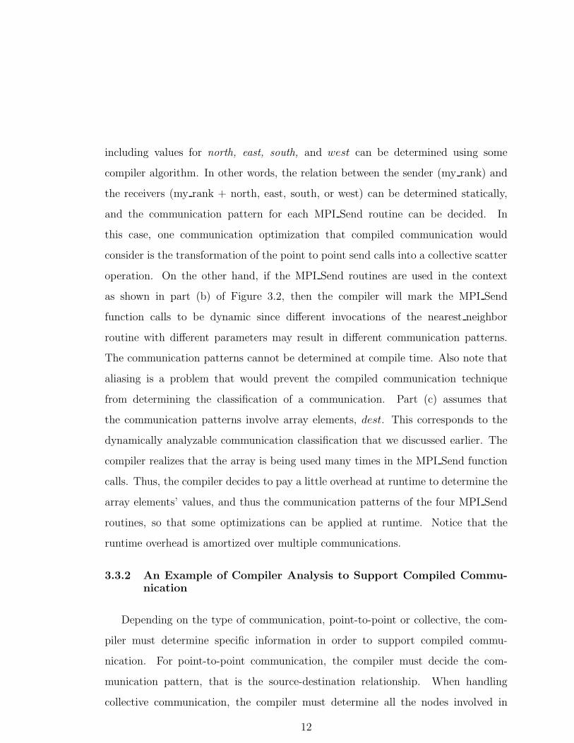
Message sizes can greatly affect the ways the communications are performed.

Figure 6.2 shows the summary of the message size distribution for collective commu-

nications in all the benchmarks. The summary is obtained by first computing the

message size distribution in terms of percentage for each range of message sizes in

each of the benchmarks. We then give equal weights to all the benchmarks that have

the particular communication and calculate the average message size distribution in

terms of percentage. The benchmarks only have one dynamically analyzable and one

dynamic collective communications, so there is not much distribution for these cases.

For static collective communications, the message sizes are mostly small (< 1KB).

This indicates that static collective communications with small message sizes are

important cases for compiled communication.

38

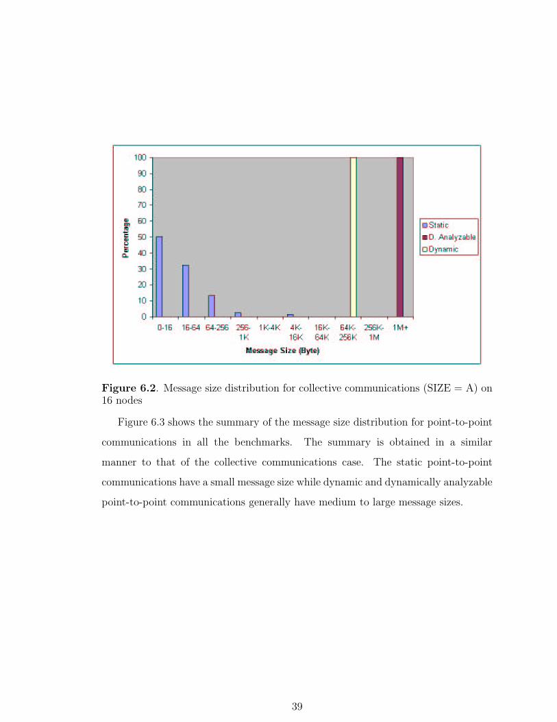
Figure 6.2. Message size distribution for collective communications (SIZE = A) on16 nodes

Figure 6.3 shows the summary of the message size distribution for point-to-point

communications in all the benchmarks. The summary is obtained in a similar

manner to that of the collective communications case. The static point-to-point

communications have a small message size while dynamic and dynamically analyzable

point-to-point communications generally have medium to large message sizes.

39

Figure 6.3. Message size distribution for point-to-point communications (SIZE =A) on 16 nodes

40

Table 6.6. Dynamic measurement for small problems (SIZE = S) on 16 nodes



Dynamic 0 0.0% 0 0.0%

Static 1 0.0% 0.03KB 0.0%

CG Dynamically analyzable 0 0.0% 0 0.0%Dynamic 47104 100.0% 225MB 100.0%

Static 100 1.5% 126KB 0.0%


Dynamic 6704 98.5% 7.83MB 100.0%

Static 3 27.3% 0.99KB 0.0%

FT Dynamically analyzable 8 72.7% 118MB 100.0%

Dynamic 0 0.0% 0 0.0%

Static 37 77.1% 0.69MB 19.4%IS Dynamically analyzable 0 0.0% 0 0.0%

Dynamic 11 22.9% 2.86MB 80.6%

Static 7 0.0% 11.1KB 0.0%BT Dynamically analyzable 23520 100.0% 0.21GB 100.0%

Dynamic 0 0.0% 0 0.0%

Static 7 0.0% 11.1KB 0.0%

SP Dynamically analyzable 38880 100.0% 0.18GB 100.0%Dynamic 0 0.0% 0 0.0%

6.2 Results for small problems on 16 nodes

In this section, we will show the results for executing the benchmarks with a

small problem size on 16 nodes. Since LU cannot be executed in this setting, we will

exclude it from the results.

Table 6.6 shows the dynamic measurement of the number and the volume for

the three types of communications in each of the benchmarks. The results are

similar to those for large problems except that a small problem size results in a

small communication volume. In terms of the volume of communications, among the

eight benchmarks, CG, MG, and IS are dominated by dynamic communications; EP

contains only static communications; FT , BT , and SP are dominated by dynamically

41

analyzable communications. Static and dynamically analyzable communications still

account for a large portion of the communications.

Table 6.7. Dynamic measurement for collective and point-to-point communicationswith small problems (SIZE = S) on 16 nodes




point-to-point 47104 225MB 100.0%

MG collective 100 126KB 1.6%point-to-point 6704 7.83MB 98.4%

FT collective 11 118MB 100.0%


IS collective 33 3.55MB 100.0%


BT collective 7 11.1KB 0.0%point-to-point 23520 209MB 100.0%

SP collective 7 11.1KB 0.0%


Table 6.7 shows the number and the volume of collective and point-to-point

communications in the benchmarks. The communications in benchmarks EP , FT ,

and IS are dominated by collective communications while the communications

in CG, MG, BT , and SP are dominated by point-to-point communications. A

smaller problem size does not significantly change the overall ratio between collective

communications and point-to-point communications in these benchmarks.

Table 6.8 shows the classification of collective communications in the benchmarks.

The results agree with previous results for large problems. The collective commu-

nications in EP , CG, MG, BT , and SP are all static. Most of the collective com-

munications in FT are dynamically analyzable. Only the collective communications

in IS are mostly dynamic. A smaller problem size does not change the distribution

of static, dynamic, and dynamically analyzable collective communications in these

benchmarks significantly.

42

Table 6.8. Dynamic measurement of collective communications with small problems(SIZE = S) on 16 nodes



Dynamic 0 0.0% 0 0.0%


Dynamic 0 0.0% 0 0.0%

Static 100 100.0% 126KB 100.0%

MG Dynamically analyzable 0 0.0% 0 0.0%Dynamic 0 0.0% 0 0.0%

Static 3 27.3% 0.99KB 0.0%

FT Dynamically analyzable 8 72.7% 118MB 100%Dynamic 0 0.0% 0 0.0%

Static 22 66.7% 692KB 19.5%

IS Dynamically analyzable 0 0.0% 0 0.0%

Dynamic 11 33.3% 2.86MB 80.5%


Dynamic 0 0.0% 0 0.0%


Dynamic 0 0.0% 0 0.0%

Table 6.9. Dynamic measurement of point-to-point communications with smallproblems (SIZE = S) on 16 nodes


Static 0 0.0% 0 0.0%


Static 0 0.0% 0 0.0%


Dynamic 6704 100.0% 7.83MB 100.0%

Static 15 100.0% 0.06KB 100.0%


Dynamic 0 0.0% 0 0.0%

Static 0 0.0% 0 0.0%BT D. ana 23520 100.0% 209MB 100.0%

Dynamic 0 0.0% 0 0.0%

Static 0 0.0% 0 0.0%

SP Dynamically analyzable 38880 100.0% 178MB 100.0%Dynamic 0 0.0% 0 0.0%

43

Table 6.9 shows the classification of point-to-point communications. As in

the cases for large problems, we see more dynamic point-to-point communications

than dynamic collective communications. CG and MG contain only dynamic

point-to-point communications. BT and SP contain only dynamically analyzable

point-to-point communications. It is even valid that none of the benchmarks has

a significant number of static point-to-point communications. The distribution of

static, dynamic, and dynamically analyzable point-to-point communications in these

benchmarks does not change when executed with a smaller problem size.

Figure 6.4 shows the summary of the message size distribution for collective

communications in all the benchmarks. The summary is obtained in the same

manner as that for large problems. The benchmarks only have one dynamically

analyzable communication, so there is not much distribution for that case. For

dynamic collective communication, the message size has a range of 1KB-4KB, and

for static ones, the message sizes are mostly small (<= 1KB). A smaller problem size

results in more small messages in collective communications. However, the trend in

the message size distribution for small problems is similar to that for large problems.

Figure 6.5 shows the summary of the message size distribution for point-to-point

communications in all the benchmarks. The summary is obtained in a similar manner

to that of large problems. We also note that a smaller problem size results in smaller

messages in point-to-point communications. However, the trend in the message size

distribution for small problems is similar to that for large problems.

44

Figure 6.4. Message size distribution for collective communications (SIZE = S) on16 nodes

Figure 6.5. Message size distribution for point-to-point communications (SIZE =S) on 16 nodes

45

6.3 Results for large problems on 4 nodes

Table 6.10. Dynamic measurement for large problems (SIZE = A) on 4 nodes


Static 5 100.0% 2.5KB 100.0%

EP Dynamically analyzable 0 0.0% 0 0.0%Dynamic 0 0.0% 0 0.0%

Static 1 0.0% 6.0B 0.0%


Static 100 3.4% 25KB 0.0%


Dynamic 2856 96.6% 512MB 100.0%

Static 3 27.3% 198B 0.0%FT Dynamically analyzable 8 72.7% 2.42GB 100.0%

Dynamic 0 0.0% 0 0.0%

Static 25 69.4% 272KB 0.1%IS Dynamically analyzable 0 0.0% 0 0.0%

Dynamic 11 30.6% 277MB 99.9%

Static 18 0.0% 5.7KB 0.3%

LU Dynamically analyzable 2016 1.6% 1.32GB 83.6%Dynamic 124008 98.4% 254MB 16.1%

Static 7 0.1% 2.2KB 0.0%

BT Dynamically analyzable 9672 99.9% 4.53GB 100.0%Dynamic 0 0.0% 0 0.0%

Static 7 0.0% 2.2KB 0.0%


Dynamic 0 0.0% 0 0.0%

Table 6.10 shows the dynamic measurement of the number and the volume for

the three types of communications in each of the benchmarks. We can see from

the table that the results show a similar trend as we have seen in the previous

cases. In terms of the volume of communications, CG, MG, and IS are dominated

by dynamic communications; EP contains only static communications; FT , BT ,

and SP are dominated by dynamically analyzable communications. LU has 83.6%

dynamically analyzable communications, 16.1% dynamic communications, and a

small percentage, 0.3%, of static communications. In general, using a smaller number

of nodes increases the total communication volume, especially for point-to-point

46

communications, but it does not significantly change the ratios among the volumes

for static, dynamic, and dynamically analyzable communications.

Table 6.11. Dynamic measurement for collective and point-to-point communica-tions with large problems (SIZE = A) on 4 nodes





MG collective 100 25.2KB 0.0%point-to-point 2856 512MB 100.0%

FT collective 11 2.42GB 100.0%


IS collective 33 277MB 100.0%


LU collective 18 5.72KB 0.0%point-to-point 126024 1.58GB 100%



SP collective 7 2.22KB 0.0%point-to-point 19272 7.9GB 100.0%

Table 6.11 shows the number and the volume of collective and point-to-point com-

munications in the benchmarks. We still obtain similar results: the communications

in benchmarks EP , FT , and IS are dominated by collective communications while

the communications in CG, MG, LU , BT , and SP are dominated by point-to-point

communications. Using a smaller number of nodes does not significantly change the

ratios between the volumes for collective and point-to-point communications.

Table 6.12 shows the classification of collective communications in the bench-

marks. EP , CG, MG, LU , BT , and SP have collective communications that

are all static while most of the collective communications in FT are dynamically

analyzable. IS still have collective communications that are mostly dynamic. The

collective communications in the benchmarks have a similar distribution among

static, dynamic, and dynamically analyzable communications with different numbers

of nodes in the system.

47

Table 6.12. Dynamic measurement of collective communications with large prob-lems (SIZE = A) on 4 nodes


Static 5 100.0% 2.5KB 100.0%


Dynamic 0 0.0% 0 0.0%


Dynamic 0 0.0% 0 0.0%

Static 100 100.0% 25.2KB 100.0%MG Dynamically analyzable 0 0.0% 0 0.0%

Dynamic 0 0.0% 0 0.0%

Static 3 27.3% 0.20KB 0.0%

FT Dynamically analyzable 8 72.7% 2.42GB 100%Dynamic 0 0.0% 0 0.0%

Static 22 66.7% 272KB 0.1%

IS Dynamically analyzable 0 0.0% 0 0.0%Dynamic 11 33.3% 278MB 99.9%

Static 18 100.0% 5.72KB 100.0%


Dynamic 0 0.0% 0 0.0%


Dynamic 0 0.0% 0 0.0%


Dynamic 0 0.0% 0 0.0%

Results of point-to-point classification are shown in Table 6.13. Again, CG

and MG contain only dynamic point-to-point communications whereas BT and

SP contain only dynamically analyzable point-to-point communications. None of

the benchmarks has a significant number of static point-to-point communications.

A smaller number of nodes does not significantly change the distribution of static,

dynamic, and dynamically analyzable point-to-point communications in these bench-

marks.

The summary of the message size distribution for collective communications in

all the benchmarks is shown in Figure 6.6. This figure shows almost identical results

to patterns when the benchmarks are run on 16 nodes with a large problem size.

48

Table 6.13. Dynamic measurement of point-to-point communications with largeproblems (SIZE = A) on 4 nodes


Static 0 0.0% 0 0.0%


Static 0 0.0% 0 0.0%

MG Dynamically analyzable 0 0.0% 0 0.0%Dynamic 2856 100.0% 512MB 100.0%

Static 3 100.0% 0.01KB 100.0%


Dynamic 0 0.0% 0 0.0%

Static 0 0.0% 0 0.0%LU Dynamically analyzable 2016 1.6% 1.32GB 83.9%

Dynamic 124008 98.4% 254MB 16.1%

Static 0 0.0% 0 0.0%BT D. ana 9672 100.0% 4.53GB 100.0%

Dynamic 0 0.0% 0 0.0%

Static 0 0.0% 0 0.0%

SP Dynamically analyzable 19272 100.0% 7.9GB 100.0%Dynamic 0 0.0% 0 0.0%

Figure 6.6. Message size distribution for collective communications (SIZE = A) on4 nodes

49

Figure 6.7. Message size distribution for point-to-point communications (SIZE =A) on 4 nodes

The message sizes for dynamic and dynamically analyzable communications become

larger, but the message size distribution has a similar trend. Figure 6.7 shows the

summary of the message size distribution for point-to-point communications in all

the benchmarks. With a smaller number of nodes, more messages are of larger sizes.

However, the message size distribution shows a similar trend: the static point-to-point

communications have a small message size while dynamic and dynamically analyzable

point-to-point communications generally have medium to large message sizes.

6.4 Results for small problems on 4 nodes

Table 6.14 shows the dynamic measurement of the number and the volume for the

three types of communications in each of the benchmarks. The table, in accordance

to previous experiments, reveals the same trend as we had before, although the

communication volume is significantly smaller. LU has 0.1% static communications,

50

Table 6.14. Dynamic measurement for small problems (SIZE = S) on 4 nodes



Dynamic 0 0.0% 0 0.0%

Static 1 0.0% 6.0B 0.0%

CG Dynamically analyzable 0 0.0% 0 0.0%Dynamic 6720 100.0% 74.7MB 100.0%

Static 100 5.3% 25KB 0.3%


Dynamic 1776 94.7% 9MB 99.7%

Static 3 27.3% 198B 0.0%

FT Dynamically analyzable 8 72.7% 75.5MB 100.0%

Dynamic 0 0.0% 0 0.0%

Static 25 69.4% 137KB 6.0%IS Dynamically analyzable 0 0.0% 0 0.0%

Dynamic 11 30.6% 2.16MB 94.0%

Static 18 0.4% 5.7KB 0.1%LU Dynamically analyzable 416 9.4% 9.58MB 86.1%

Dynamic 4008 90.2% 1.54MB 13.8%

Static 7 0.2% 2.2KB 0.0%

BT Dynamically analyzable 2952 99.8% 57.3MB 100.0%Dynamic 0 0.0% 0 0.0%

Static 7 0.1% 2.2KB 0.0%

SP Dynamically analyzable 4872 99.9% 59.2MB 100.0%

Dynamic 0 0.0% 0 0.0%

86.1% dynamically analyzable communications, and 13.8% dynamic communications

in terms of the volume of communication. CG, MG, and IS are still dominated by

dynamic communications; EP contains only static communications; FT , BT , and

SP are dominated by dynamically analyzable communications.

We show the number and the volume of collective and point-to-point communi-

cations for each benchmarks in Table 6.15. The table also shows the same trend

as we had in previous executions with different problem sizes and different numbers

of nodes. The communications in benchmarks EP , FT , and IS are dominated by

collective communications while the communications in CG, MG, LU , BT , and SP

are dominated by point-to-point communications.

51

Table 6.15. Dynamic measurement for collective and point-to-point communica-tions with small problems (SIZE = S) on 4 nodes




point-to-point 6720 74.7MB 100.0%

MG collective 100 25.2KB 0.3%point-to-point 1776 9.00MB 99.7%

FT collective 11 75.5MB 100.0%


IS collective 33 2.3MB 100.0%point-to-point 3 0.01KB 0.0%

LU collective 18 5.72KB 0.0%

point-to-point 4424 11.1MB 100%


point-to-point 2952 57.3MB 100.0%

SP collective 7 2.22KB 0.0%point-to-point 4872 59.2MB 100.0%

52

Table 6.16. Dynamic measurement of collective communications with small prob-lems (SIZE = S) on 4 nodes


Static 5 100.0% 2.5KB 100.0%


Dynamic 0 0.0% 0 0.0%


Dynamic 0 0.0% 0 0.0%

Static 100 100.0% 25.2KB 100.0%MG Dynamically analyzable 0 0.0% 0 0.0%

Dynamic 0 0.0% 0 0.0%

Static 3 27.3% 0.20KB 0.0%

FT Dynamically analyzable 8 72.7% 75.5MB 100%Dynamic 0 0.0% 0 0.0%

Static 22 66.7% 137KB 6.0%

IS Dynamically analyzable 0 0.0% 0 0.0%Dynamic 11 33.3% 2.16MB 94.0%

Static 18 100.0% 5.72KB 100.0%


Dynamic 0 0.0% 0 0.0%


Dynamic 0 0.0% 0 0.0%


Dynamic 0 0.0% 0 0.0%

Table 6.16 shows the classification of collective communications in the bench-

marks. Even this table shows a similar trend as in other collective communications

tables before. Among the benchmarks, EP , CG, MG, LU , BT , and SP have

collective communications that are all static. One benchmark, FT , had collective

communications that are dynamically analyzable. Only the collective communica-

tions in IS are mostly dynamic.

Table 6.17 shows the classification of point-to-point communications. The trend

in this table is similar to that in previous results: none of the benchmarks has a

significant number of static point-to-point communications; CG and MG contain

53

Table 6.17. Dynamic measurement of point-to-point communications with smallproblems (SIZE = S) on 4 nodes


Static 0 0.0% 0 0.0%

CG Dynamically analyzable 0 0.0% 0 0.0%

Dynamic 6720 100.0% 74.7MB 100.0%

Static 0 0.0% 0 0.0%MG Dynamically analyzable 0 0.0% 0 0.0%

Dynamic 1776 100.0% 9.00MB 100.0%

Static 3 100.0% 0.01KB 100.0%IS Dynamically analyzable 0 0.0% 0 0.0%

Dynamic 0 0.0% 0 0.0%

Static 0 0.0% 0 0.0%

LU Dynamically analyzable 416 9.40% 9.59MB 86.2%Dynamic 4008 90.6% 1.54MB 13.8%

Static 0 0.0% 0 0.0%

BT D. ana 2952 100.0% 57.3MB 100.0%Dynamic 0 0.0% 0 0.0%

Static 0 0.0% 0 0.0%

SP Dynamically analyzable 4872 100.0% 59.2MB 100.0%

Dynamic 0 0.0% 0 0.0%

only dynamic point-to-point communications; BT and SP contain only dynamically

analyzable point-to-point communications.

Figure 6.8 shows the summary of the message size distribution for collective

communications in all the benchmarks. The benchmarks have only one large message

size (1MB+) for dynamically analyzable communication, so there is not much

distribution for the dynamically analyzable case. About 95% of the messages for

dynamic communications are in the range of 16KB-64KB while 5% are in the range

of 4KB-16KB. For static collective communications, the message sizes are mostly

small (< 1KB). Figure 6.9 shows the summary of the message size distribution

for point-to-point communications in all the benchmarks. As in previous results,

the static point-to-point communications have a small message size while dynamic

and dynamically analyzable point-to-point communications generally have medium

to large message sizes.

54

Figure 6.8. Message size distribution for collective communications (SIZE = S) on4 nodes

Figure 6.9. Message size distribution for point-to-point communications (SIZE =S) on 4 nodes

55

CHAPTER 7

CONCLUSIONS

We studied the communication characteristics in the MPI implementation of

the NAS parallel benchmarks and investigated the feasibility and effectiveness of

compiled communication on MPI programs. The results of this study can also be

used by other compiler assisted approaches to improve communication performance.

The main conclusions are the followings:

• Static and dynamically analyzable communications account for a significant

portion of the communications in the benchmarks, which indicates that com-

piled communication can be effective if it can optimize these two types of

communications.

• The majority of collective communications are static, which indicates that

compiled communication should be applied to optimize MPI collective com-

munications. Furthermore, most static collective communications have small

message sizes.

• There is a significant number of dynamically analyzable point-to-point com-

munications in the benchmarks. For compiled communication to be effective

in handling MPI point-to-point communications, it must be able to optimize

dynamically analyzable communications.

• While different problem sizes and different numbers of nodes in the system

affect the sizes of messages in the communications, they do not significantly

56

change the distribution and the ratio of static, dynamic, and dynamically

analyzable communications in the benchmarks. Thus, the above conclusions

hold for different problem sizes and different numbers of nodes in the system.

57

REFERENCES

[1] Mario Lauria and Andrew Chien. MPI-FM: High Performance MPI onWorkstation Clusters. Journal of Parallel and Distributed Computing. 40(1):4-18, 10 January 1997.

[2] A. Basu, V. Buch, W. Vogels, and T. von Eicken. U-Net: A User-LevelNetwork Interface for Parallel and Distributed Computing. Proceedings of the15th ACM SIGOPS Symposium on Operating Systems Principles, OperatingSystems Review. 29(5):40-53, December 1995.

[3] The MPI Forum. The mpi-2: Extensions to the message passing inter-face. Technical report, http://www.mpi-forum.org/docs/mpi-20-html/mpi2-report.html, July, 1997.

[4] Alfred V. Aho, Ravi Sethi, and Jeffrey D. Ullman. Compilers: Principles,Techniques, and Tools. Addison Wesley, Reading, Massachusetts, 1988.

[5] Steven S. Muchnick. Advanced Compiler Design and implementation. MorganKaufmann, San Francisco, CA, p. 232, 1997.

[6] D. H. Bailey, T. Harris, R. Van der Wigngaart, W. Saphir, A. Woo, and M.Yarrow. The nas parallel benchmarks 2.0. Technical report, NASA AmesResearch Center, 1995.

[7] F. Cappello and D. Etiemble. Mpi versus mpi+openmp on ibm sp forthe nas benchmarks. SC’00: High Performance Networking and ComputingConference, 2000.

[8] D. Lahaut and C. Germain. Static communications in parallel scientificprograms. Parle94 LNCS 817, pages 262–276, 1994.

[9] P. Banerjee, J. Chandy, M. Gupta, E. Hodge, J. Holm, A. Lain, D. Palermo,S. Ramaswamy, and E. Su. The Paradigm Compiler for Distributed-MemoryMulticomputers. IEEE Computer, 28(10):37–47, 1995.

[10] Seema Hiranandani, Ken Kenney, Charles Koelbel, Ulrich Kremer, and Chau-Wen Tseng. An Overview of the Fortran D Programming System. In FourthInternational Workshop on Languages and Compilers for Parallel Computing,pages 18-34, Santa Clara, CA, 1991.

58

[11] NAS Parallel Benchmarks, available at http://www.nas.nasa.gov/NAS/NPB.

[12] F. Wong, R. Martin, R. Arpaci-Dusseau, and D. Culler. Architectural require-ments of scalability of the nas parallel benchmarks. SC’99: High PerformanceNetworking and Computing Conference, 1999.

[13] J.S. Vetter and F. Mueller. Communication characteristics of large-scalescientific applications for contemporary cluster architectures. InternationalParallel and Distributed Processing Symposium, 2002.

[14] Xin Yuan, Rajiv Gupta, and Rami Melhem. Demand-driven data flow analysisfor communication optimization. Parallel Processing Letters, 7:359–370, Dec,1997.

[15] Xin Yuan, Scott Daniels, Ahmad Faraj, and Amit Karwande. Group man-agement schemes for implementing mpi collective communication over ip-multicast. In 6th International Conference on Computer Science and Infor-matics, pages 309-313. JCIS2002, 2002.

[16] Udaya Ranawake. Performance Comparison of the Three Subclustersof the HIVE. http://webserv.gsfc.nasa.gov/neumann/hive comp/bmarks/bmarks.html.

59

BIOGRAPHICAL SKETCH

Ahmad A. Faraj

Ahmad Faraj was born on March 26, 1976 in Kuwait. He received his Bachelor of

Science degree in Computer Science from Florida State University in 2000. After

completing his Masters of Science degree, he plans to pursue a doctoral degree in

Computer Science at Florida State University.

60

communication characteristics in the nas ...xyuan/paper/faraj-thesis.pdfthe members of the committee...

Documents